Saturation Physics and Deuteron–Gold Collisions at RHIC

Abstract

We present a review of parton saturation/Color Glass Condensate physics in the context of deuteron-gold ($d+Au$) collisions at RHIC. Color Glass Condensate physics is a universal description of all high energy hadronic and nuclear interactions. It comprises classical (McLerran-Venugopalan model and Glauber-Mueller rescatterings) and quantum evolution (JIMWLK and BK equations) effects both in small-$x$ hadronic and nuclear wave functions and in the high energy scattering processes. Proton-nucleus (or $d+A$) collisions present a unique opportunity to study Color Glass Condensate predictions, since many relevant observables in proton-nucleus collisions are reasonably well-understood theoretically in the Color Glass Condensate approach. In this article we review the basics of saturation/Color Glass Condensate physics and reproduce derivations of many important observables in proton (deuteron)–nucleus collisions. We compare the predictions of Color Glass physics to the data generated by $d+Au$ experiments at RHIC and observe an agreement between the data and the theory, indicating that Color Glass Condensate has probably been discovered at RHIC. We point out further experimental measurements which need to be carried out to test the discovery.

Prepared for publication in Prog. Part. Nucl. Phys.

1 Introduction

Saturation/Color Glass Condensate physics [1]-[24] is a rapidly developing field of strong interactions at high energy. Color Glass Condensate (CGC) physics describes high parton densities inside the hadronic and nuclear wave functions at small values of Bjorken $x$ variable. It demonstrates how the gluon fields in the hadronic and nuclear wave functions reach their maximum allowable values in quantum chromodynamics (QCD) corresponding to $A_{\mu}\sim 1/g$ [3, 4, 5, 6]. The CGC formalism is also successfully applied to calculation of total, elastic and diffractive cross sections of high energy hadronic and nuclear scattering. There, by resumming the strong gluon field dynamics, it resolves such long-standing questions as unitarity of the scattering $S$-matrix [25] and infrared (IR) safety [26], which are known to be violated by the Balitsky-Fadin-Kuraev-Lipatov (BFKL) evolution equation [27] corresponding to the weak field limit of CGC. Saturation/CGC approach allows one to calculate particle production in hadronic and nuclear scattering [28]-[44]. The resulting inclusive particle production cross sections are infrared-safe, which is a significant theoretical improvement over the IR-divergent perturbative QCD results [45, 46] making the small coupling approach to particle production self-consistent. One of the interesting application of particle production in CGC framework is understanding the initial conditions for the evolution of the quark-gluon system produced in heavy ion collisions toward the possible thermalization leading to formation of quark-gluon plasma (QGP) [41, 42, 43, 44].

Perturbative QCD (pQCD) has been extremely successful in describing the particle production data over a large kinematic window [47]. Applications of pQCD to particle production in high energy hadronic or nuclear collisions are based on the use of collinear factorization theorems. The essence of a collinearly factorized cross section is the idea of incoherence. In other words, a hadronic cross section can be written as a convolution of parton distributions and fragmentation functions, which are universal non-perturbative objects that are also subject to perturbative evolution (DGLAP), with a hard scattering cross section involving partons, which is perturbatively calculable but is process dependent. Parton distribution functions are typically measured in Deep Inelastic Scattering experiments such as the ones performed at HERA, where it has been observed that the gluon and sea quark distributions grow very fast with decreasing Bjorken $x$. This fast growth can be understood in pQCD as driven by radiation of gluons with small Bjorken $x$ via DGLAP evolution equations. Collinear factorization theorems are not exact and are violated by effects that are typically suppressed by inverse of the hard momentum transfer but can be enhanced by energy (or $\ln\,1/x$) or $A$ dependent factors, which may be large at high energy and/or for large nuclei. This necessitates construction of a new formalism that does not rely on collinear factorization and can include these potentially large effects. The hint for this new formalism comes from pQCD itself, noticing that the rise of parton distribution functions can not continue for ever since it would lead to growth of hadronic cross sections at a rate which would violate unitarity. A weak coupling mechanism which can tame this fast growth is gluon recombination and saturation. Color Glass Condensate formalism is the natural generalization of pQCD in order to make it applicable to dense partonic systems.

The extensive theoretical progress in the field of saturation/Color Glass has been summarized in several review articles, mostly concentrating on the issues of non-linear small-$x$ evolution [48, 49, 50]. Our article here deals with saturation/Color Glass Condensate physics putting more emphasis on particle production in proton (deuteron)–nucleus collisions ($p(d)A$) and in deep inelastic scattering (DIS). Many of the relevant particle production observables in $pA$ and DIS have been well-understood theoretically in the saturation/Color Glass approach, at least at the partonic level [28]-[40]. It is therefore, very important to be able to verify our theoretical understanding by comparing the predictions of CGC physics for particle production in $p(d)A$ to the experimental data produced by deuteron-gold ($d+Au$) scattering program at Relativistic Heavy Ion Collider (RHIC) at Brookhaven National Laboratory (BNL) [51]-[60]. Below we will review both the CGC predictions [61]-[65] and experimental data reported by RHIC experiments [54]-[60]. We will point out the apparent agreement between the two indicating a possible discovery of Color Glass Condensate at RHIC [31]. We will also review future experimental test which can be carried out to test the CGC discovery both by $d+Au$ program at RHIC and by $pA$ scattering program at Large Hadron Collider (LHC) at CERN.

The paper is structured as follows. We begin in Sect. 2 with a general review of saturation/CGC physics. This review is by no means all-inclusive: we will concentrate on the material that we will need later in our discussion of particle production. We refer the interested reader who wants to learn more about various aspects of small-$x$ evolution to the dedicated reviews in [48, 49, 50, 66]. In Sect. 2.1 we discuss the BFKL evolution equation [27] along with its problems, such as violation of unitarity [25] and diffusion into infrared [26]. We also review the Gribov-Levin-Ryskin–Mueller-Qiu (GLR-MQ) evolution equation [1, 2]. We proceed in Sect. 2.2 by discussing quasi-classical approximation in small-$x$ physics. We review Glauber-Mueller multiple rescatterings in DIS [67, 68] and McLerran-Venugopalan model of small-$x$ wave functions of large nuclei [3, 4, 5, 6, 69]. Quasi-classical regime at small-$x$ is valid when $x$ is small enough, so that coherent interactions of nucleons in the nucleus with the projectile are possible. This translates into the requirement for parton coherence length $l_{coh}$ to be larger than the nuclear radius $R$ [70],

$$l_{coh}\,=\,\frac{1}{2\,m_{N}\,x_{Bj}}\,>\,R,$$ (1)

with $m_{N}$ the nucleon mass and $x_{Bj}$ the Bjorken $x$ variable of a parton. Defining the rapidity variable $Y=\ln 1/x_{Bj}$ we recast the condition (1) as $Y\,>\,\ln A$, with $A$ the atomic number of the nucleus. On the other hand, when $x_{Bj}$ becomes too small, BFKL evolution effects become important, breaking down the quasi-classical approximation. BFKL evolution brings in powers of $\alpha_{s}\,\ln(1/x_{Bj})\,\sim\,\alpha_{s}\,Y$. Requiring for such effects to be small, $\alpha_{s}\,Y<1$, we obtain an upper bound on the allowable rapidity range. The applicability window for the quasi-classical approximation is then

$$\ln A\,\leq\,Y\,\leq\,\frac{1}{\alpha_{s}}.$$ (2)

We also discuss in Sect. 2.2 how the saturation scale $Q_{s}$ arises in the quasi-classical limit.

We continue our review of saturation/Color Glass physics by re-deriving the Jalilian-Marian–Iancu–McLerran–Weigert–Leonidov–Kovner (JIMWLK) [7]-[10], [13]-[16] and Balitsky-Kovchegov (BK) [23, 24] non-linear evolution equations in Sect. 2.3. Quantum small-$x$ evolution corrections become important when $\alpha_{s}\,Y\,{{}_{\displaystyle{>}}\atop\displaystyle{\sim}}\,1$ [27], such that

$$Y\,\geq\,\frac{1}{\alpha_{s}}.$$ (3)

Eq. (3) gives a lower bound on the region of applicability of JIMWLK and BK evolution equations.

We conclude the review of CGC by solving the non-linear evolution equations in Sect. 2.4. There we discuss the solution of linear (BFKL) evolution equation outside of the saturation region, demonstrate an interesting property of the solution of JIMWLK and BK known as geometric scaling inside the saturation region [71, 72] and reproduce the derivation of extended geometric scaling outside of that region [73]. We demonstrate how saturation scale $Q_{s}$ grows with energy once the quantum evolution effects are included [74, 75, 76]. We explain how JIMWLK and BK evolution equations resolve the problems of the BFKL evolution by unitarizing the corresponding total cross sections of DIS and by prohibiting diffusion into the infrared, making the small-coupling approximation self-consistent [77]-[81].

We continue in Sect. 3 by deriving expressions for a number of particle production observables in $pA$ collisions in the saturation/CGC framework. We start in Sect. 3.1 by calculating inclusive gluon production cross section in $pA$ in the quasi-classical approximation [32, 82, 33, 83]. We show that quasi-classical multiple rescatterings lead to Cronin enhancement [84] of gluon production in $pA$ [64, 62, 85]-[89], as can be seen from Fig. 36. We then proceed in Sect. 3.2 by including the effects of quantum BK evolution in the expression for gluon production cross section in $pA$ [34, 90, 91]. As one can see from Fig. 41, the effect of small-$x$ evolution is to flatten the Cronin maximum introducing suppression of particle production at all transverse momenta $p_{T}$ (see Fig. 41) [61]-[64, 81, 92]. In Sect. 3.3 we calculate valence quark production cross section in $pA$ both in the quasi-classical limit and including small-$x$ evolution [37]-[40]. We move on to electromagnetic probes in Sect. 3.4, where we calculate prompt photon and dilepton production cross sections in $pA$ collisions [93]-[100]. Finally, in Sect.3.5 we analyze two-particle correlations [101]-[110]. We rederive production cross section in $pA$ for two gluons at mid-rapidity [103], for a quark and a gluon at forward rapidity [103] and for $q\bar{q}$ pair at mid-rapidity [105]-[110].

We review some of the data generated by $d+Au$ scattering program at RHIC [51]-[60] in Sect. 4. We show that the data reported by BRAHMS [57], PHENIX [51], PHOBOS [52] and STAR [53] experiments show Cronin-like enhancement of particle production at mid-rapidity. We discuss how this result, combined with suppression of produced hadrons in $Au+Au$ collisions [111]-[114], serves as a control experiment for the signals of quark-gluon plasma formation in heavy ion collisions at RHIC [115]-[120]. We then review BRAHMS data at forward rapidity [56, 57], indicating suppression predicted by saturation/CGC approach [61, 62, 63]. This data is confirmed by preliminary results from PHENIX [59], PHOBOS [58] and STAR [60], demonstrating that Color Glass Condensate has probably been discovered at RHIC [120]. We conclude Sect. 4 by listing future experimental tests [121, 122, 123] which need to be carried out to verify the discovery of CGC at RHIC [120].

We conclude in Sect. 5 by discussing some of the issues which we inevitably had to leave out in this review, including recent progress in our understanding of pomeron loop corrections to small-$x$ evolution [124]-[128] and some exclusive processes [129]-[132], which can not be measured at RHIC.

Throughout the paper we will use the following notation for the 4-vectors: for a 4-vector $v_{\mu}=(v_{0},v_{1},v_{2},v_{3})$ we define the light cone components by $v^{\pm}=(v_{0}\pm v_{3})/\sqrt{2}$ and combine the transverse components into a two-dimensional vector ${\underline{v}}=(v_{1},v_{2})$. The metric tensor is chosen in such a way that $v_{\mu}v^{\mu}=2\,v^{+}\,v^{-}-{\underline{v}}^{2}$.

2 Overview of Saturation/Color Glass Condensate Physics

In this Section we will review the developments and advances of high energy QCD which led to our modern understanding of the saturation/Color Glass Condensate physics.

2.1 Early Developments

2.1.1 The BFKL Equation

A milestone in the development of small-$x$ physics was the derivation by Balitsky, Fadin, Kuraev, and Lipatov of what has become known as the BFKL equation [27]. The BFKL equation describes the behavior of scattering amplitudes and gluon distribution functions at asymptotically high energies. It does it by resumming leading logarithms of energy, i.e., powers of the parameter $\alpha_{s}\ln s$, where in the perturbative QCD regime the coupling constant is small, $\alpha_{s}\ll 1$, and, in Regge kinematics, the center of mass energy $s$ of the scattering process is much larger than any other momentum scale involved.

Derivation of the BFKL equation is rather complicated. For derivations in the transverse momentum space we refer the interested reader to [27, 133], as well as to Sect. 2.3.1 below. Derivation in transverse coordinate space can be found in [19, 20, 21, 22], as well as in Sect. 2.3.2 below. Here we are going to present a simple physical picture of the BFKL evolution following Mueller in [134].

Physical Picture
 
Consider an ultrarelativistic gluon scattering on a target at rest. Before scattering on the target, the gluon can emit one or more extra gluons. The emissions are illustrated in Fig. 1. In the infinite momentum frame considered here, the gluon moving in the light cone “+” direction has a very large typical light cone “+” component of its momentum, which we denote by $p^{+}$. The original gluon emits another gluon with a much smaller light cone momentum $k_{1}^{+}\ll p^{+}$. A simple calculation shows that the emission probability is given by

$$dP_{1}\,=\,\frac{\alpha_{s}\,N_{c}}{\pi}\,\frac{d^{2}k_{1}}{{\underline{k}}_{1}^{2}}\,\frac{dk_{1}^{+}}{k_{1}^{+}},$$ (4)

where $N_{c}$ is the number of colors (and the $SU(N_{c})$ Casimir operator in the adjoint representation) and ${\underline{k}}_{1}$ is the two-component transverse momentum vector of the gluon $\#1$. Eq. (4) can be obtained from the usual formula for photon Bremsstrahlung by multiplying it with the color Casimir $N_{c}$ and replacing $\alpha_{EM}\rightarrow\alpha_{s}$. Following [134] we assume that all emitted gluons have fixed transverse momentum of the order of some scale $Q$. This allows us to simplify the problem by replacing the transverse momentum integral $d^{2}k_{1}/{\underline{k}}_{1}^{2}$ by a constant $c$. Defining the rapidity variable

$$y_{1}\,=\,\ln\frac{p^{+}}{k_{1}^{+}}$$ (5)

we rewrite Eq. (4) as

$$dP_{1}\,=\,c\,\frac{\alpha_{s}\,N_{c}}{\pi}\,dy_{1}.$$ (6)

Using Eq. (6) we conclude that given the rapidity interval

$$\Delta y_{1}\,=\,\frac{\pi}{\alpha_{s}\,c\,N_{c}}$$ (7)

the original gluon would split into two gluons with probability 1.

To generalize the picture to many gluon emissions, we have to understand the space-time picture of the process. First we note that the typical light cone coherence time of the gluon $\#1$ is

$$\tau_{1}\,\equiv\,x^{+}_{1}\,=\,\frac{2\,k_{1}^{+}}{{\underline{k}}_{1}^{2}}\,\approx\,\frac{2\,k_{1}^{+}}{Q^{2}}.$$ (8)

Similarly, for the $i$th gluon in the gluon cascade, the light cone time is of the order of

$$\tau_{i}\,\approx\,\frac{2\,k_{i}^{+}}{Q^{2}}.$$ (9)

Thus, if the original gluon emits a cascade of gluons with their longitudinal momenta being progressively smaller

$$p^{+}\gg k_{1}^{+}\gg k_{2}^{+}\gg\ldots\gg k_{N}^{+}$$ (10)

than their light cone times would also be ordered

$$\tau_{1}\gg\tau_{2}\gg\ldots\gg\tau_{N}.$$ (11)

Figure 1: Gluon cascade leading to the BFKL evolution. All gluon emissions are ordered in light cone “+” momenta, and, correspondingly, in light cone time.

This cascade is shown in Fig. 1. There the gluons are ordered in time, such that the typical coherence time of each emitted gluon is much shorter than the coherence times of all the preexisting (harder) gluons. Therefore, for the $i$th gluon, all the gluons $1,\ldots,i-1$ appear frozen in time. The gluon can be emitted off any of these preexisting gluons, which is shown by disconnected gluon lines in Fig. 1. Indeed, in the transverse direction the gluons are coherent only over short distances of the order of $\Delta x_{\perp}\sim 1/Q$, such that each gluon is emitted only by some fraction $c^{\prime}$ of the preexisting gluons. Since the colors of all these gluons are random, the $i$th gluon “sees” an effective color charge

$$g_{i}\,=\,\sqrt{c^{\prime}\,i}\,g$$ (12)

which results from a random walk in color space of $i$ preexisting gluons. The probability of $i$th gluon emission is

$$dP_{i}\,=\,c\,c^{\prime}\,i\,\frac{\alpha_{s}\,N_{c}}{\pi}\,dy_{i}.$$ (13)

The rapidity interval required for $i$th gluon emission is

$$\Delta y_{i}\,=\,\frac{\pi}{c\,c^{\prime}\,i\,\alpha_{s}\,N_{c}}.$$ (14)

Thus, the rapidity needed to emit $N$ gluons is given by

$$Y_{N}\,=\,\sum_{i=1}^{N}\Delta y_{i}\,=\,\frac{\pi}{c\,c^{\prime}\,\alpha_{s}\,N_{c}}\,\sum_{i=1}^{N}\,\frac{1}{i}\,\approx\,\frac{\pi}{c\,c^{\prime}\,\alpha_{s}\,N_{c}}\,\ln N,$$ (15)

so that the total number of gluons emitted in rapidity interval $Y$ is given by

$$N(Y)\,=\,e^{c\,c^{\prime}\,\frac{\alpha_{s}\,N_{c}}{\pi}\,Y}.$$ (16)

This simple physical picture that we borrowed from [134] gives the right qualitative behavior of the BFKL evolution. The exact BFKL evolution also leads to the exponentially increasing number of gluons, just like we obtained in Eq. (16). The successive time ordered emissions discussed above and shown in Fig. 1 resum the leading logarithms of energy, just like the exact BFKL equation: each power of $\alpha_{s}$ gets enhanced by a power of rapidity $Y$ (which is equivalent to the logarithm of center of mass energy $s$), such that Eq. (16) resums powers of $\alpha_{s}Y$. Even the kinematics of successive emissions considered above (see Eq. (10)) is the same as in the exact BFKL evolution, where extracting the leading logarithmic contribution requires ordering of the gluons’ longitudinal momenta. 

The BFKL Equation 

Let us now consider a scattering of a bound heavy quark-antiquark state (quarkonium, or simply onium) on another quarkonium. The interaction between the onia is shown in Fig. 2.

Figure 2: Scattering of two onia with the interaction mediated by the BFKL evolution.

In general, we can write down the total onium-onium scattering cross section as a convolution of the onia light cone wave functions [135, 136] with the imaginary part of the forward scattering amplitude of two quark-antiquark pairs (the imaginary part is denoted by $F$)

$$\sigma_{tot}\,=\,2\,\int d^{2}x\,\int_{0}^{1}dz\,\int d^{2}x^{\prime}\,\int_{0}^{1}dz^{\prime}\,\Phi_{q\bar{q}}(\underline{x},z)\,\Phi_{q\bar{q}}(\underline{x}^{\prime},z^{\prime})\,F({\underline{x}},{\underline{x}}^{\prime},Y),$$ (17)

where $\Phi_{q\bar{q}}(\underline{x},z)$ and $\Phi_{q\bar{q}}(\underline{x}^{\prime},z^{\prime})$ are light cone wave functions of the onia with transverse sizes ${\underline{x}}$ and ${\underline{x}}^{\prime}$. In the center of mass frame, each of the onia carries a large light cone momentum, $p^{+}$ and $p^{\prime-}$ correspondingly. For high energy eikonal scattering considered here, these two momenta ($p^{+}$ and $p^{\prime-}$) are much larger than any transverse momentum scales in the problem. In each of the onia the quark carries the fraction $z$ (or $z^{\prime}$) of the light cone component of the total momentum of the quark-antiquark state. $Y=\ln(s/4M^{2})$ is the rapidity variable, defined as a logarithm of the ratio of the center of mass energy of the onium-onium scattering $s$ over some typical transverse momentum scale, like the onium mass $M$ used here.

At the lowest order the interaction in Fig. 2 is mediated by the two-gluon exchange. The corresponding imaginary part of the forward amplitude, which we denote by $F=F^{(0)}$, is given by

$$F^{(0)}(\underline{x},\underline{x}^{\prime})\,=\,\frac{\alpha_{s}^{2}\,C_{F}}{N_{c}}\,\int\,\frac{d^{2}l}{[\underline{l}^{2}]^{2}}\,(2-e^{-i\underline{l}\cdot\underline{x}}-e^{i\underline{l}\cdot\underline{x}})\,(2-e^{-i\underline{l}\cdot\underline{x}^{\prime}}-e^{i\underline{l}\cdot\underline{x}^{\prime}}),$$ (18)

where $C_{F}=(N_{c}^{2}-1)/2N_{c}$ is the $SU(N_{c})$ Casimir operator in the fundamental representation and ${\underline{l}}$ is the transverse momentum of each of the gluons.

The BFKL evolution allows one to calculate quantum corrections to Eq. (18) that bring in powers of $\alpha_{s}Y$. Apparently, as was shown in [27], such corrections preserve the two-gluon exchange structure of the interactions and can be summarized by the blob in Fig. 2. Corresponding generalization of the amplitude (18) reads

$$F({\underline{x}},{\underline{x}}^{\prime},Y)\,=\,\frac{\alpha_{s}^{2}\,C_{F}}{N_{c}}\,\int\,\frac{d^{2}l\,d^{2}l^{\prime}}{\underline{l}^{2}\,{\underline{l}}^{\prime 2}}\,(2-e^{-i\underline{l}\cdot\underline{x}}-e^{i\underline{l}\cdot\underline{x}})\,(2-e^{-i\underline{l}^{\prime}\cdot\underline{x}^{\prime}}-e^{i\underline{l}^{\prime}\cdot\underline{x}^{\prime}})\,f({\underline{l}},{\underline{l}}^{\prime},Y)$$ (19)

with ${\underline{l}}$ and ${\underline{l}}^{\prime}$ the gluons’ transverse momenta on both sides of the blob as shown in Fig. 2. At the lowest (two-gluon) order the amplitude $f({\underline{l}},{\underline{l}}^{\prime},Y)$ is given by a delta-function

$$f^{(0)}({\underline{l}},{\underline{l}}^{\prime})\,=\,f({\underline{l}},{\underline{l}}^{\prime},Y=Y_{0})\,=\,\delta^{2}({\underline{l}}-{\underline{l}}^{\prime}),$$ (20)

which, after substitution into Eq. (19) readily gives Eq. (18). ($Y_{0}$ is some initial rapidity, corresponding to the center of mass energy where the two-gluon exchange dominates the interaction.)

The BFKL equation for the amplitude $f({\underline{l}},{\underline{l}}^{\prime},Y)$ with the initial condition (20) reads [27]

$$\frac{\partial f({\underline{l}},{\underline{l}}^{\prime},Y)}{\partial Y}\,=\,\frac{\alpha_{s}\,N_{c}}{\pi^{2}}\int\!\frac{d^{2}k}{(\underline{k}-\underline{l})^{2}}\left[f(\underline{k},\underline{l}^{\prime},Y)-\frac{{\underline{l}}^{2}\,f(\underline{l},\underline{l}^{\prime},Y)}{{\underline{k}}^{2}+(\underline{k}-\underline{l})^{2}}\right].$$ (21)

Figure 3: Schematic representation of a single rung of the BFKL evolution.

The equation is illustrated in Fig. 3, where the dashed vertical line denotes the cut. The equation in Fig. 3 states that the blob can either consist of just a two gluon exchange without any evolution (the first term on the right hand side of Fig. 3), corresponding to the initial condition in Eq. (20), or the blob may have small-$x$ evolution corrections included. The evolution corrections can be real (the second term on the right in Fig. 3) and virtual (the third and fourth terms on the right of Fig. 3). The real term contains a gluon in the final state (crossing the cut) and corresponds to the first term on the right hand side of Eq. (21). The gluon is emitted off the $t$-channel gluons via the effective Lipatov vertices [27], denoted by thick dots in Fig. 3, which represent the sum of all possible emissions. The virtual terms in Fig. 3 contain no gluon in the final state and correspond to the last term on the right of Eq. (21).

Figure 4: BFKL evolution as a ladder diagram.

The solution of the BFKL equation should contain all iterations of the kernel depicted in Fig. 3. Iterating the BFKL kernel leads to the ladder diagrams, like the one shown in Fig. 4. It depicts interaction of two onia characterized by typical transverse momentum scales $Q_{1}$ and $Q_{2}$ interacting via a BFKL-evolved amplitude. Fig. 4 shows the structure of the blob in Fig. 2 in more detail. Again, the triple gluon vertices in Fig. 4 are not the usual QCD vertices: they are effective Lipatov vertices responsible for the real part of the BFKL kernel [27]. Similarly, the $t$-channel gluon lines do not correspond to the usual QCD gluon propagators: they give the so-called reggeized gluon propagators [27].

The emissions resummed by a Lipatov vertex are shown in Fig. 5. There we consider scattering of two ultrarelativistic quarks leading to production of a soft gluon with momentum $k^{+}\ll p^{+}$ and $k^{-}\ll p^{\prime-}$ [27, 45, 28, 29, 30, 31]. The correct emission amplitude, which is obtained by summing diagrams A-E in Fig. 5, can be written as the first diagram in Fig. 5 with the effective vertex triple gluon given by [27, 46]

$$C_{\mu}^{a}(k,\underline{q})\,=\,g\,T^{a}\,\left(\frac{\underline{q}^{2}}{k^{-}}-k^{+}\,,\,-\frac{(\underline{k}-\underline{q})^{2}}{k^{+}}+k^{-}\,,\,2\underline{q}-\underline{k}\right)$$ (22)

in the $(+,-,\perp)$ form with $T^{a}$ the $SU(N_{c})$ color matrix in the adjoint representation.

Figure 5: The diagrams contributing to effective Lipatov vertex, which is denoted by a very thick dot.

To construct an effective reggeized gluon propagator one has to resum all leading logarithmic corrections to a single $t$-channel gluon exchange keeping the exchange amplitude in a color octet state. The details of this sophisticated resummation procedure can be found in [137]. Here we will only give the final result: the leading logarithmic corrections to the $t$-channel gluon propagator exponentiate, modifying the gluon propagator

$$\frac{D_{\mu\nu}^{ab}(q)}{q^{2}}\,\longrightarrow\,\frac{D_{\mu\nu}^{ab}(q)}{q^{2}}\,e^{-\omega({\underline{q}}^{2})\,\Delta y}$$ (23)

where $\omega({\underline{q}}^{2})$ is the gluon Regge trajectory [27, 46]

$$\omega({\underline{q}}^{2})\,=\,\frac{\alpha_{s}\,N_{c}}{(2\pi)^{2}}\,\int\,\frac{d^{2}k\,{\underline{q}}^{2}}{{\underline{k}}^{2}({\underline{k}}-{\underline{q}})^{2}}$$ (24)

and $\Delta y$ is the rapidity interval spanned by a given $t$-channel gluon.

Eqs. (22) and (23) give us the rules for vertices and $t$-channel propagators necessary to construct the ladder diagram in Fig. 4. There the leading logarithmic contribution is given by the multi-Regge kinematics of the produced $s$-channel gluons

$$p^{+}\,\gg\,k_{1}^{+}\,\gg\,k_{2}^{+}\,\gg\,\ldots\,\gg\,k_{N}^{+}\,\gg\,p^{\prime+},$$ (25)

$$p^{-}\,\ll\,k_{1}^{-}\,\ll\,k_{2}^{-}\,\ll\,\ldots\,\ll\,k_{N}^{-}\,\ll\,p^{\prime-},$$ (26)

and

$$k_{1}^{\perp}\,\sim\,k_{2}^{\perp}\,\sim\,\ldots\,\sim\,k_{N}^{\perp},$$ (27)

where $k_{i}^{\perp}=|{\underline{k}}_{i}|$.

Solution of the BFKL Equation

To solve Eq. (21) we first have to find the eigenfunctions of its integral kernel. The kernel of BFKL equation is conformally invariant. It is easy to verify that a complete and orthogonal set of eigenfunctions of Eq. (21) is formed by the functions [27, 138]

$$({\underline{l}}^{2})^{-\frac{1}{2}+i\nu}\,e^{i\,n\,\phi},$$ (28)

where $\phi$ is the angle between vector ${\underline{l}}$ and some chosen axes and $n$ is integer. The eigenvalues of the eigenfunctions in Eq. (28) are [27, 138]

$$\frac{2\,\alpha_{s}\,N_{c}}{\pi}\,\chi(n,\nu)$$ (29)

where

$$\chi(n,\nu)\,=\,\psi(1)-\frac{1}{2}\psi\left(\frac{1+|n|}{2}+i\nu\right)-\frac{1}{2}\psi\left(\frac{1+|n|}{2}-i\nu\right)$$ (30)

with $\psi(z)=d\ln\Gamma(z)/dz$. Denoting $l\equiv|{\underline{l}}|$ and $l^{\prime}\equiv|{\underline{l}}^{\prime}|$ we write the solution of Eq. (21) as

$$f({\underline{l}},{\underline{l}}^{\prime},Y)\,=\,\sum_{n=-\infty}^{\infty}\,\int_{-\infty}^{\infty}\,d\nu\,C_{n,\nu}(Y)\,l^{-1+2i\nu}\,l^{\prime-1-2i\nu}\,\,e^{i\,n\,(\phi-\phi^{\prime})}.$$ (31)

Substituting Eq. (31) into Eq. (21) and using the eigenvalues from Eq. (29) we find

$$C_{n,\nu}(Y)\,=\,C_{n,\nu}^{(0)}\ e^{\frac{2\,\alpha_{s}\,N_{c}}{\pi}\,\chi(n,\nu)\,Y},$$ (32)

where the coefficient $C_{n,\nu}^{(0)}$ is fixed by the initial conditions (20) giving

$$C_{n,\nu}^{(0)}\,=\,\frac{1}{2\pi^{2}}.$$ (33)

Combining Eqs. (32), (33) and (31) yields

$$f({\underline{l}},{\underline{l}}^{\prime},Y)\,=\,\frac{1}{2\pi^{2}}\,\sum_{n=-\infty}^{\infty}\,\int_{-\infty}^{\infty}\,d\nu\,e^{\frac{2\,\alpha_{s}\,N_{c}}{\pi}\,\chi(n,\nu)\,Y}\,l^{-1+2i\nu}\,l^{\prime-1-2i\nu}\,\,e^{i\,n\,(\phi-\phi^{\prime})}.$$ (34)

Eq. (34) provides us the solution of Eq. (21) with the initial conditions given by Eq. (20). As one can see already from Eq. (34), the BFKL equation generates amplitudes which grow exponentially with rapidity $Y$. Remembering that $Y\sim\ln s$, this translates into a power of energy growth.

Let us evaluate the amplitude in Eq. (34) a little further. Consider the case when $l\sim l^{\prime}$, i.e., the two momentum scales involved in the problem are not very much different from each other. A simple analysis of the function $\chi(n,\nu)$ allows one to conclude that the dominant contribution to the amplitude is given by the $n=0$ term in the sum in Eq. (34). Expanding $\chi(n=0,\nu)$ around the saddle point at $\nu=0$ we get

$$\chi(0,\nu)\,\approx\,2\ln 2-7\,\zeta(3)\,\nu^{2},$$ (35)

where $\zeta(z)$ is the Riemann zeta-function. Using Eq. (35) in Eq. (34) we can perform the $\nu$-integration obtaining [27]

$$f({\underline{l}},{\underline{l}}^{\prime},Y)\,\approx\,\frac{1}{2\,\pi^{2}\,l\,l^{\prime}}\,\sqrt{\frac{\pi}{14\,\zeta(3)\,\overline{\alpha}_{s}\,Y}}\ \exp\left[(\alpha_{P}-1)\,Y-\frac{\ln^{2}l/l^{\prime}}{14\,\zeta(3)\,\overline{\alpha}_{s}\,Y}\right],$$ (36)

where we have defined the intercept of the perturbative pomeron

$$\alpha_{P}-1\,=\,\frac{4\,\alpha_{s}\,N_{c}}{\pi}\,\ln 2$$ (37)

and

$$\overline{\alpha}_{s}\,\equiv\,\frac{\alpha_{s}\,N_{c}}{\pi}.$$ (38)

The essential feature of Eq. (36) is that it shows that cross sections mediated by the BFKL exchange grow as a power of energy

$$\sigma\,\sim\,e^{(\alpha_{P}-1)\,Y}\,\sim\,s^{\alpha_{P}-1}.$$ (39)

This behavior is reminiscent of the Pomeranchuk singularity in the reggeon calculus, and is, therefore, sometimes referred to as the pomeron or the hard pomeron (to distinguish it from the soft non-perturbative interaction phenomenon).

Figure 6: Diffusion of the gluon transverse momentum in the BFKL ladder. Non-perturbative region is denoted by the scale $\Lambda$.

Problems of the BFKL Evolution

The BFKL equation poses some important questions even in the case of heavy onium-onium scattering and at the leading order in $\alpha_{s}$ in the kernel.

(i) The power of energy growth of the total cross section (Eq. (39)) violates Froissart unitarity bound, which states that the growth of the total cross sections with energy at asymptotically high energies is bounded by [25]

$$\sigma\,\leq\,\frac{const}{m_{\pi}^{2}}\,\ln^{2}s$$ (40)

with $m_{\pi}$ the pion’s mass. (For a good pedagogical derivation of the Froissart bound we refer the readers to [66].) This implies that some new physical effects should modify the BFKL equation at very large $s$ making the resulting amplitude unitary.

(ii) The solution in Eq. (34) includes a diffusion term, which is the last term in its exponent. To see the potential danger of this term, let us consider a half of the ladder of Fig. 4, stretching from one of the onia (the top one) to some intermediate gluon in the middle of the ladder carrying transverse momentum $l_{\perp}$ and having rapidity $Y/2$. Applying Eq. (36) to that half-ladder we see that it includes a term

$$\exp\left[-{\ln^{2}(l/Q_{1})\over 14\,\zeta(3)\,\overline{\alpha}_{s}\,\,(Y/2)}\right].$$ (41)

This term is responsible for diffusion of the transverse momenta from the initial perturbative scale $Q_{1}$ both to high and low momenta, i.e., into infrared and ultraviolet. It implies that the distribution of gluons’ transverse momentum in the ladder, while still centered around $Q_{1}$, may have significant fluctuations towards high and low momenta $l$ as shown in Fig. 6, where we plot the typical range of transverse momentum $l$ in the ladder of Fig. 4 as a function of rapidity of gluons in the ladder. The width of the diffusion grows with rapidity $Y$ allowing for larger fluctuations at higher energies. Thus, no matter how large the starting scale $Q_{1}$ is, at certain very high energy the momentum of some gluons in the middle of the ladder would become of the order of $\Lambda_{QCD}$ leading to the coupling constant $\alpha_{s}(\Lambda_{QCD})\sim 1$ and thus invalidating further application of perturbative QCD ($\alpha_{s}\ll 1$) and, consequently, of the BFKL evolution [26]. The diffusion starts from the scale $Q_{1}$ at one end of the ladder and from the scale $Q_{2}$ at the other end (see Fig. 6). At high energy the allowed momentum range broadens towards the middle and touches the non-perturbative region of low momenta at mid-rapidity. The plot of allowed momenta as a function of rapidity shown here in Fig. 6 is sometimes referred to as Bartels cone [26]. Again it hints that the BFKL equation should be modified at higher energies to avoid the problem of running into the non-perturbative region. Alternatively, if such modification is not found within perturbation theory, we would be forced to admit that high energy asymptotics is dominated by non-perturbative physics. Fortunately this is not the case, as will be shown below.

2.1.2 The GLR-MQ Equation

As we have seen above, the BFKL evolution leads to exponential growth of total cross sections with energy, violating the Froissart bound [25]. It also leads to exponential growth of the density of partons in the onium (or hadron) wave function. To see this let us define an unintegrated gluon distribution of an onium by

$$\phi(x_{Bj},{\underline{k}}^{2})\,=\,\frac{\alpha_{s}\,C_{F}}{\pi}\,\int\,\frac{d^{2}l}{\underline{l}^{2}}\,(2-e^{-i\underline{l}\cdot\underline{x}}-e^{i\underline{l}\cdot\underline{x}})\,f({\underline{l}},{\underline{k}},Y=\ln 1/x_{Bj})\,d^{2}x\,dz\,\Phi_{q\bar{q}}({\underline{x}},z).$$ (42)

The definition (42) is illustrated in Fig. 7. To obtain it we have, essentially, truncated the lower onium in Fig. 2, leaving two disconnected gluon lines. The diagram in Fig. 7 has to be calculated in $A^{+}=0$ light cone gauge to give the gluon distribution function. The unintegrated gluon distribution function in Eq. (42) gives us the number of gluons in the onium wave function having transverse momentum ${\underline{k}}$ and carrying the fraction $x_{Bj}$ of the onium “+” component of the momentum (Bjorken, or Feynman $x$).

Figure 7: Unintegrated gluon distribution of an onium.

Using the BFKL solution from Eq. (36) in Eq. (42) one can easily see that the gluon distribution grows as

$$\phi(x_{Bj},{\underline{k}}^{2})\,\sim\,\left(\frac{1}{x_{Bj}}\right)^{\alpha_{P}-1}.$$ (43)

Therefore, the number of gluons rises sharply at small $x$ / high energy, in agreement with the semi-qualitative estimate of Eq. (16). This feature is illustrated qualitatively by the gluon cascade representation of the BFKL evolution presented in the Sect. 2.1.1. There, the gluons are produced in a multi-Regge kinematics with comparable transverse momenta (see Eq. (27)). That means that the typical transverse sizes of the gluons, given by $r_{i}^{\perp}\sim 1/k_{i}^{\perp}$ are also of the same order for all the gluons

$$r_{1}^{\perp}\,\sim\,r_{2}^{\perp}\,\sim\,\ldots\,\sim\,r_{N}^{\perp}.$$ (44)

Therefore, the BFKL cascade produces many gluons in the onium or hadron wave function, with roughly the same transverse size. As energy increases, more and more gluons are produced in the cascade. The gluons overlap in the transverse plane, creating areas of high gluon density. Thus, not only the number of gluons, but their density in the transverse plane increase with energy.

Figure 8: BFKL equation as a high density machine.

This is illustrated in Fig. 8 for a wave function of a proton. At some initial value of Bjorken $x$, corresponding to lower energy, the proton’s wave function may have one parton with transverse size $\sim 1/Q$ in it. As we go to smaller $x$, BFKL evolution would generate many more partons of comparable size, creating a region of high gluon density in the wave function [134].

However, the gluon density can not rise forever. It is known that in QCD the gluon fields can not be stronger than $A_{\mu}\sim 1/g$ for small coupling $g$. Therefore, when the gluon field reaches the density corresponding to field strength

$$\frac{F_{\mu\nu}}{Q^{2}}\,\sim\,\frac{1}{g}$$ (45)

some new, possibly non-linear effects should become important slowing down the density growth [134]. This strong field constraint may be intimately connected to the problem of unitarization of cross sections at fixed impact parameter, i.e., to the black disk limit (see below).

To understand how the growth of the gluon distribution can be tamed, Gribov, Levin and Ryskin (GLR) [1, 139] considered distribution functions of a “dense” proton or a nucleus. By “dense” proton we imply a model of a proton filled with sources of color charge — sea quarks and gluons, which were pre-created in the proton’s wave function by some non-perturbative mechanism (see, e.g., [140]). Gribov, Levin and Ryskin [1, 139] argued that for such systems multiple ladder exchanges may become important. Since one is interested in gluon distribution, which is a correlation function for two gluonic fields, these multiple ladders should come in as the so-called “fan” diagrams. An example of a fan diagram is shown in Fig. 9.

Figure 9: An example of fan diagram resummed by the GLR-MQ equation.

There multiple BFKL ladders start from different quarks and gluons in the proton or nucleus, shown by straight lines at the bottom of Fig. 9. Due to high density of gluon fields, the ladders can not stay independent forever. As the energy increases so does the gluon density, eventually leading to recombination of the ladders, as shown in Fig. 9. Ladder recombination is described by effective ladder merger vertices, denoted by blobs in Fig. 9. These vertices are sometimes called the triple pomeron vertices, since they connect three different ladders (BFKL pomerons). For their calculation we refer the reader to [141] and references therein.

Gribov, Levin and Ryskin [1, 139] suggested that, before the energy gets sufficiently high for all nonlinear effects to become important, there could be an intermediate energy region where the physics of gluon distributions is dominated by $2\rightarrow 1$ ladder recombination only. This recombination brought in a quadratic correction to the linear BFKL equation, leading to the GLR evolution equation [1, 139]

$$\frac{\partial\,\phi(x,{\underline{k}}^{2})}{\partial\ln(1/x)}\,=\,\frac{\alpha_{s}\,N_{c}}{\pi^{2}}\int\!\frac{d^{2}l}{(\underline{k}-\underline{l})^{2}}\left[\phi(x,\underline{l}^{2})-\frac{{\underline{k}}^{2}\,\phi(x,\underline{k}^{2})}{{\underline{l}}^{2}+(\underline{k}-\underline{l})^{2}}\right]-\frac{\alpha_{s}^{2}\,\pi}{S_{\perp}}\,\left[\phi(x,\underline{k}^{2})\right]^{2},$$ (46)

where, for simplicity, we assumed that the proton or nucleus has a shape of a cylinder oriented along the beam axis with the cross sectional area $S_{\perp}=\pi R^{2}$. As expected, the linear term in Eq. (46) is equivalent to the BFKL equation (21), while the quadratic term, responsible for ladder mergers, introduces damping, thus slowing down the growth of the gluon distributions with energy. The growth of gluon distributions with energy given by Eq. (46) should slow down and saturate at very high energies. This phenomenon became known as the saturation of parton distributions.

The ansatz (46) of GLR [1] was proven by Mueller and Qiu [2] in the double leading logarithmic approximation (DLA) for the (integrated) gluon distribution functions, which are defined as [2]

$$xG(x,Q^{2})\,=\,\int^{Q^{2}}\,dk^{2}\,\phi(x,k^{2}).$$ (47)

The double logarithmic approximation is a resummation of the powers of the parameter

$$\alpha_{s}\ln(1/x)\ln(Q^{2}/\Lambda^{2}).$$ (48)

The BFKL equation [27] was derived in the leading logarithmic approximation (LLA), corresponding to resummation of the parameter $\alpha_{s}\ln 1/x$, or, equivalently, $\alpha_{s}Y$ (see Sect. 2.1.1). In the limiting case of large $Q^{2}$ in the distribution functions (or large ${\underline{k}}^{2}$ in the unintegrated distribution functions) another large logarithm becomes important: $\ln Q^{2}/\Lambda^{2}$, where $\Lambda$ is the non-perturbative QCD scale. It becomes possible to define a new resummation parameter, $\alpha_{s}\ln(1/x)\ln(Q^{2}/\Lambda^{2})$. In principle, the LLA is much broader than DLA: it resums powers of $\alpha_{s}\ln 1/x$ with any dependence of the obtained terms on $Q^{2}$, not restricting it to the leading logarithmic regime. Leading powers of $\alpha_{s}\ln(Q^{2}/\Lambda^{2})$ are, of course, resummed by the Dokshitzer, Gribov, Lipatov, Altarelli, Parisi (DGLAP) equation [142]. Indeed, the DLA limits of the BFKL and DGLAP equations are identical, since they are resumming the same parameter, $\alpha_{s}\ln(1/x)\ln(Q^{2}/\Lambda^{2})$.

Employing the DLA and analyzing diagrams with two merging DGLAP ladders, Mueller and Qiu arrived at the following evolution equation [2] (again written here for a cylindrical nucleus)

$$\frac{\partial^{2}\,xG(x,Q^{2})}{\partial\ln(1/x)\,\partial\ln(Q^{2}/\Lambda^{2})}\,=\,\frac{\alpha_{s}\,N_{c}}{\pi}\,xG(x,Q^{2})-\frac{\alpha_{s}^{2}\,\pi}{S_{\perp}}\,\frac{1}{Q^{2}}\,[xG(x,Q^{2})]^{2},$$ (49)

which is known as GLR-MQ equation. Eq. (49) is in agreement with Eq. (46), and could be be obtained from the latter by taking the DLA limit and using Eq. (47). Thus Mueller and Qiu [2] proved Eq. (46) in the double logarithmic limit.

Eq. (49) allows one to estimate at which $Q^{2}$ the non-linear saturation effects become important. To do that we have to equate the linear and quadratic terms on the right hand side of Eq. (49). The corresponding value of $Q^{2}$ is called the saturation scale and is denoted by $Q_{s}^{2}$. It is determined by

$$Q_{s}^{2}\,=\,\frac{\alpha_{s}\,\pi^{2}}{S_{\perp}\,N_{c}}\,xG(x,Q_{s}^{2}).$$ (50)

The non-linear saturation effects are important for all $Q\,{{}_{\displaystyle{<}}\atop\displaystyle{\sim}}\,Q_{s}$, which is known as the saturation region.

The quadratic damping term in both Eq. (46) and Eq. (49) was believed to be important only near the border of the saturation region, for $Q\sim Q_{s}$, where the non-linear effects were only starting to become important [1, 2]. It was expected that higher order non-linear corrections would show up as one goes deeper into the saturation region towards $Q<Q_{s}$ (see, e.g., [143]). In the next Section we will talk about the model where all such corrections could be resummed in a particular quasi-classical approximation, where the BFKL evolution can be neglected.

2.2 Quasi-Classical Approximation

As was suggested by the GLR equation, the effects of high gluonic field strengths come in as multiple exchanges. To better understand the effect of multiple rescatterings one can consider a specific model of hadronic or nuclear wave functions. In this section we will consider the case of deep inelastic scattering on a large dilute nucleus, where multiple rescatterings take place on individual nucleons and, as we will demonstrate, can be described by the Glauber-Mueller formula [67]. In the infinite momentum frame this large nucleus can be thought of as a Lorentz-contracted “pancake” in the direction transverse to its velocity. Due to a large number of nucleons in the nucleus, the parton color charge density fluctuations in this “pancake” are large, described by a hard scale referred to as the saturation scale $Q_{s}$. For very large nuclei, the saturation scale is large $Q_{s}\gg\Lambda_{QCD}$ making the strong coupling constant small $\alpha_{s}(Q_{s})\ll 1$. At weak coupling the dynamics of field theories becomes classical: therefore, as was concluded by McLerran and Venugopalan [3], the gluon field of such a large ultrarelativistic nucleus should be given by the solution of the classical Yang-Mills equations of motion [144] with the nucleus providing the source current. The resulting small-$x$ nuclear wave function systematically includes all multiple rescatterings and exhibits the effects of saturation.

2.2.1 Glauber-Mueller Rescatterings

Figure 10: Deep inelastic scattering in the rest frame of the target.

Let us consider deep inelastic scattering (DIS) on a large nucleus. In DIS the incoming electron emits a virtual photon, which in turn interacts with the proton or nucleus. In the rest frame of the nucleus, the interaction can be thought of as virtual photon splitting into a quark-antiquark pair, which then interacts with the nucleus (see Fig. 10). Since the light cone lifetime of the $q\bar{q}$ pair is much longer than the size of the target nucleus, the total cross section for the virtual photon–nucleus scattering can be written as a convolution of the virtual photon’s light cone wave function (the probability for it to split into a $q\bar{q}$ pair) with the forward scattering amplitude of a $q\bar{q}$ pair interacting with the nucleus

$$\sigma_{tot}^{\gamma*A}(Q^{2},x_{Bj})\,=\,\int\frac{d^{2}x\,dz}{2\pi}\,[\Phi_{T}({\underline{x}},z)+\Phi_{L}({\underline{x}},z)]\ d^{2}b\ N({\underline{x}},{\underline{b}},Y)$$ (51)

with the help of the light-cone perturbation theory [135, 136]. Here the incoming photon with virtuality $Q$ splits into a quark–antiquark pair with the transverse separation ${\underline{x}}$ and the impact parameter (transverse position of the center of mass of the $q\bar{q}$ pair) ${\underline{b}}$. $Y$ is the rapidity variable given by $Y=\ln(s\,x_{T}^{2})\approx\ln 1/x_{Bj}$. The square of the light cone wave function of $q\overline{q}$ fluctuations of a virtual photon is denoted by $\Phi_{T}({\underline{x}},z)$ and $\Phi_{L}({\underline{x}},z)$ for transverse and longitudinal photons correspondingly, with $z$ being the fraction of the photon’s longitudinal momentum carried by the quark. At the lowest order in electromagnetic coupling ($\alpha_{EM}$) $\Phi_{T}({\underline{x}},z)$ and $\Phi_{L}({\underline{x}},z)$ are given by [145, 130]

$$\Phi_{T}({\underline{x}},z)=\frac{2N_{c}}{\pi}\,\sum_{f}\alpha^{f}_{EM}\,\left\{a_{f}^{2}\ K_{1}^{2}(x_{T}a_{f})\ [z^{2}+(1-z)^{2}]+m_{f}^{2}K_{0}(x_{T}a_{f})^{2}\right\},$$ (52)

$$\Phi_{L}({\underline{x}},z)=\frac{2N_{c}}{\pi}\,\sum_{f}\alpha^{f}_{EM}\,\ 4\,Q^{2}\,z^{2}(1-z)^{2}\ K_{0}^{2}(x_{T}a_{f}),$$ (53)

with $a_{f}^{2}=Q^{2}z(1-z)+m_{f}^{2}$, $x_{T}=|{\bf x}|$ and $\sum_{f}$ denoting the sum over all relevant quark flavors with quark masses denoted by $m_{f}$. $\alpha^{f}_{EM}=e_{f}^{2}/4\pi$ with $e_{f}$ the electric charge of a quark with flavor $f$.

Our goal is to calculate the forward scattering amplitude of a quark–anti-quark dipole interacting with the nucleus, which is denoted by $N({\underline{x}},{\underline{b}},Y)$ in Eq. (51), including all multiple rescatterings of the dipole on the nucleons in the nucleus. To do this we need to construct a model of the target nucleus. Following Mueller [67] we assume that the nucleons are dilutely distributed in the nucleus. Let us chose to perform calculations in the $\partial_{\mu}A^{\mu}=0$ covariant gauge. There we can represent the dipole-nucleus interaction as a sequence of successive dipole-nucleon interactions, as shown in Fig. 11. Since each nucleon is a color singlet, the lowest order dipole-nucleon interaction in the forward amplitude from Fig. 11 is a two-gluon exchange. The exchanged gluon lines in Fig. 11 are disconnected at the top: this denotes a summation over all possible connections of these gluon lines either to the quark or to the anti-quark lines in the incoming dipole.

Figure 11: Deep inelastic scattering in the quasi-classical Glauber-Mueller approximation in $\partial_{\mu}A^{\mu}=0$ gauge.

Figure 12: An example of a diagram which does not contribute to the total dipole-nucleus cross section due to incorrect ordering of interactions with nucleons ($x_{2}^{+}>x_{1}^{+}$).

To demonstrate that the ordered gluon exchanges of Fig. 11 are indeed the only possible interactions, let us consider a diagram where such ordering is broken, as shown in Fig. 12. There, for simplicity, we consider scattering of a single quark on a pair of nucleons, denoted as $\#1$ and $\#2$, with interchanged ordering of quark-nucleon rescatterings. To show that such diagrams are suppressed in the dilute nucleus case, let us consider the scattering in the center of mass frame, where the projectile quark is moving in the light cone “$+$” direction and the nucleus is moving in the light cone “$-$” direction. In a dilute nucleus all the nucleons are spatially separated. For a nucleus moving in the light cone “$-$” direction this translates into a separation between the nucleons along the “$+$” axis: specifically, let us denote $x_{1}^{+}$ and $x_{2}^{+}$ the light cone coordinates of the nucleons $\#1$ and $\#2$ in Fig. 12, choosing $x_{2}^{+}>x_{1}^{+}$ for certainty. (As we will see, the opposite ordering will be indeed allowed.) We are interested in the integration over the $l$-momentum in the diagram of Fig. 12. More specifically, we are interested in integrating over the “$-$” component of this momentum. In the high energy scattering case considered here, the incoming projectile quark carries large momentum $k^{+}$, and the nucleons in the nucleus carry a large “$-$” component of momentum, e.g., $p^{\prime-}$ carried by a quark in the nucleon $\#1$. In such eikonal approximation the quark-gluon vertices do not depend on $l$, so that all the $l$-dependence is given by the gluon propagators for the $l$ and $q-l$ lines, and by the quark propagator of the $k+q-l$ line. By requiring that the outgoing quark in the nucleon $\#1$ is on mass-shell, $(p^{\prime}-l)^{2}=0$ for massless quarks, we obtain $0=(p^{\prime}-l)^{2}\approx-2p^{\prime-}l^{+}$, such that with the eikonal accuracy $l^{+}=0$. This means that the propagator of the $l$-line, given in general by $-i/l^{2}$, becomes $i/{\underline{l}}^{2}$ and does not depend on $l^{-}$ anymore. Similarly one can show that the propagator for the $q-l$-line is $i/({\underline{q}}-{\underline{l}})^{2}$ and is also independent of $l^{-}$. Thus all the $l^{-}$-dependence of the diagram in Fig. 12 is given by the denominator of the propagator of the $k+q-l$ quark line, since the numerator also becomes $l^{-}$-independent in the eikonal limit. The relevant $l^{-}$ integral can be written as

$$\int_{-\infty}^{\infty}\frac{dl^{-}}{(k+q-l)^{2}+i\epsilon}\,e^{-i\,l^{-}\,(x_{2}^{+}-x_{1}^{+})}.$$ (54)

Since $k^{+}$ is very large, we rewrite Eq. (54) as

$$\int_{-\infty}^{\infty}\frac{dl^{-}}{2\,k^{+}\,(k^{-}+q^{-}-l^{-})-({\underline{k}}+{\underline{q}}-{\underline{l}})^{2}+i\epsilon}\,e^{-i\,l^{-}\,(x_{2}^{+}-x_{1}^{+})}.$$ (55)

Since $k^{+}>0$ the integrand in Eq. (55) has a pole in the upper half plane. However, as $x_{2}^{+}>x_{1}^{+}$, the exponent in Eq. (55) allows us to close the integration contour in the lower half plane only. Therefore expression in Eq. (55) is zero, which means that the diagram in Fig. 12 can be neglected in the eikonal limit. (In fact, Eq. (55) dictates which ordering of the nucleons is allowed: if $x_{2}^{+}<x_{1}^{+}$ the expression in Eq. (55) becomes non-zero, bringing us back to ordered picture of interactions shown in Fig. 11.)

Figure 13: Diagrams contributing to dipole-nucleon scattering at the two-gluon order.

To resum the diagrams like the one shown in Fig. 11 we start by calculating the graphs contributing to the scattering of a dipole on a single nucleon, as shown in Fig. 13. Remembering that we are working in the $\partial_{\mu}A^{\mu}=0$ gauge and assuming for the moment that all scattering in the nucleon happens on one of its valence quarks we write for the sum of the diagrams in Fig. 13 (similarly to Eq. (18))

$$\frac{\alpha_{s}^{2}\,C_{F}}{N_{c}}\,\int\frac{d^{2}l}{[{\underline{l}}^{2}]^{2}}\,(2-e^{-i{\underline{l}}\cdot{\underline{x}}}-e^{i{\underline{l}}\cdot{\underline{x}}}),$$ (56)

where ${\underline{x}}$ is the transverse separation between the quark and the anti-quark in the incoming dipole, as shown in Fig. 13. Instead of performing the integration in Eq. (56) exactly, let us note that gluon are correct degrees of freedom responsible for the interactions only if the dipole is much smaller than the typical nucleon size, $x_{\perp}\ll 1/\Lambda$, with $\Lambda$ some non-perturbative infrared cutoff. Expanding the argument of the integral in Eq. (56) and integrating over ${\underline{l}}$ we obtain (see also [116])

$$\frac{\alpha_{s}^{2}\,\pi\,C_{F}}{N_{c}}\,x_{\perp}^{2}\,\int_{\Lambda}^{1/x_{\perp}}\frac{dl_{T}}{l_{T}}\,=\,\frac{\alpha_{s}^{2}\,\pi\,C_{F}}{N_{c}}\,x_{\perp}^{2}\,\ln\frac{1}{x_{\perp}\,\Lambda}.$$ (57)

As one can show by explicitly calculating the diagram in Fig. 7 without the evolution (or by using Eq. (20) in Eq. (42), replacing $q\bar{q}$ dipole by a valence quark in the latter, and using the resulting unintegrated gluon distribution in Eq. (47)), at the lowest two-gluon order the gluon distribution function of a valence quark is given by

$$x_{Bj}G(x_{Bj},Q^{2})\,=\,\frac{\alpha_{s}\,C_{F}}{\pi}\,\ln\frac{Q^{2}}{\Lambda^{2}}.$$ (58)

Using Eq. (58) in Eq. (57) yields

$$\frac{\alpha_{s}\,\pi^{2}}{2\,N_{c}}\,x_{\perp}^{2}\,x_{Bj}G(x_{Bj},1/x_{\perp}^{2}).$$ (59)

Eq. (59) can be easily generalized to the case of a nucleon by using the gluon distribution of a nucleon $xG_{N}$ in it instead of that of a valence quark

$$\frac{\sigma^{q{\bar{q}}N}}{2}\,=\,\frac{\alpha_{s}\,\pi^{2}}{2\,N_{c}}\,x_{\perp}^{2}\,x_{Bj}G_{N}(x_{Bj},1/x_{\perp}^{2}).$$ (60)

Eq. (60) gives us the scattering cross section of a quark dipole on a single nucleon. The factor of $2$ is due to the definition of total cross section in terms of the forward scattering amplitude, as shown in Eq. (17).

To obtain the multiple rescattering amplitude of Fig. 11 we have to resum all multiple rescatterings of Fig. 13 (or, equivalently, Eq. (60)). Defining the $S$-matrix of a quark–anti-quark pair scattering on a nucleus at rest by $S(z,{\underline{x}})$, where $z$ is the longitudinal coordinate of the pair as it propagates through nuclear matter with $z=0$ at the edge of the nucleus, we can write the following equation

$$\frac{\partial}{\partial z}S(z,{\underline{x}})\,=\,-\frac{\rho\,\sigma^{q{\bar{q}}N}}{2}S(z,{\underline{x}})$$ (61)

with $\rho$ the density of nucleons in the nucleus ($\rho=A/[(4/3)\pi R^{3}]$ for a spherical nucleus of radius $R$ with atomic number $A$.) Eq. (61) has the following physical meaning: as the dipole propagates through the nucleus it may encounter nucleons, with the probability of interaction per unit path length $dz$ given by the product of nucleon density $\rho$ and the interaction probability $\sigma^{q{\bar{q}}N}/2$ from Eq. (60). (In the literature devoted to jet quenching in the medium this quantity is referred to as opacity [118, 119].) The initial condition for Eq. (61) is given by a freely propagating dipole without interactions, such that $S(z=0,{\underline{x}})=1$. We refer the interested reader to [116, 32, 117] for a more detailed derivation of Eq. (61). Solving Eq. (61) with $S(z=0,{\underline{x}})=1$ initial condition yields

$$S(z,{\underline{x}})\,=\,\exp\left\{-\frac{\rho\,\sigma^{q{\bar{q}}N}}{2}\,z\right\}.$$ (62)

To construct the forward scattering amplitude $N$ of a dipole scattering on a nucleus we need to know the $S$-matrix for the dipole which went through the whole nucleus. To obtain it we need to put $z=T({\underline{b}})$ in Eq. (62), where $T({\underline{b}})$ is the nuclear profile function equal to the length of the nuclear medium at a given impact parameter $\underline{b}$, such that $T({\underline{b}})=2\,\sqrt{R^{2}-{\underline{b}}^{2}}$ for a spherical nucleus of radius $R$. Identifying $N({\underline{x}},{\underline{b}},Y)$ with the scattering $T$-matrix, such that $N=1-S$ we finally write [67]

$$N({\underline{x}},{\underline{b}},Y=0)\,=\,1-\exp\left\{-\frac{\rho\,\sigma^{q{\bar{q}}N}}{2}\,T({\underline{b}})\right\}\,=\,1-\exp\left\{-\frac{\alpha_{s}\,\pi^{2}}{2\,N_{c}}\,\rho\,T({\underline{b}})\,x_{\perp}^{2}\,x_{Bj}G_{N}(x_{Bj},1/x_{\perp}^{2})\right\}.$$ (63)

This expression is known as Glauber-Mueller formula [68, 67], since it presents a generalization of the Glauber model of independent multiple rescatterings in the nucleus [68] to the case of QCD [67].

We put $Y=0$ in the argument of $N$ in Eq. (63) to underline that this expression does not include any small-$x$ evolution which would bring in the rapidity dependence. Indeed, Eq. (63) was derived in the approximation where the interaction of the dipole with each of the nucleons is limited to a two-gluon exchange. At this order the gluon distribution $x_{Bj}G_{N}$ is given by Eq. (58) and is, therefore, $x_{Bj}$-independent, leading to rapidity-independence of the whole expression in Eq. (63).

Eq. (63) allows us to determine the parameter corresponding to the resummation of the diagrams like the one shown in Fig. 11. Using the gluon distribution from Eq. (58) in Eq. (63), and noting that for large nuclei the profile function scales as $T({\underline{b}})\sim A^{1/3}$ and the nucleon density scales as $\rho\sim A^{0}$, we conclude that the resummation parameter of multiple rescatterings is [5]

$$\alpha_{s}^{2}\,A^{1/3}.$$ (64)

The physical meaning of the parameter $\alpha_{s}^{2}\,A^{1/3}$ is rather straightforward: at a given impact parameter the dipole interacts with $\sim A^{1/3}$ nucleons exchanging two gluons with each. Since the two-gluon exchange is parametrically of the order $\alpha_{s}^{2}$ we obtain $\alpha_{s}^{2}\,A^{1/3}$ as the resummation parameter.

Figure 14: The forward amplitude of the dipole–nucleus scattering $N$ plotted as a function of the transverse separation between the quark and the anti-quark in a dipole $x_{\perp}$ using Eq. (66).

Defining the quark saturation scale

$$Q_{s}^{2}({\underline{b}})\,\equiv\,\frac{4\,\pi\,\alpha_{s}^{2}\,C_{F}}{N_{c}}\,\rho\,T({\underline{b}})$$ (65)

we rewrite Eq. (63) as

$$N({\underline{x}},{\underline{b}},Y=0)\,=\,1-\exp\left\{-\frac{x_{\perp}^{2}\,Q_{s}^{2}({\underline{b}})\,\ln(1/x_{T}\,\Lambda)}{4}\,\right\}.$$ (66)

The dipole amplitude $N$ from Eq. (66) is plotted (schematically) in Fig. 14 as a function of $x_{\perp}$. One can see that, at small $x_{\perp}$, $x_{\perp}\ll 1/Q_{s}$, we have $N\sim x_{\perp}^{2}$ and the amplitude is a rising function of $x_{\perp}$. However, at large dipole sizes $x_{\perp}{{}_{\displaystyle{>}}\atop\displaystyle{\sim}}1/Q_{s}$, the growth stops and the amplitude levels off (saturates) at $N=1$. This regime corresponds to the black disk limit for the dipole-nucleus scattering: for large dipoles the nucleus appears as a black disk. To understand that $N=1$ regime corresponds to the black disk limit let us note that the total dipole-nucleus scattering cross section is given by

$$\sigma^{q{\bar{q}}A}_{tot}\,=\,2\,\int d^{2}b\,N({\underline{x}},{\underline{b}},Y)$$ (67)

where the integration goes over the cross sectional area of the nucleus. If $N=1$ at all impact parameters $\underline{b}$ inside the nucleus, Eq. (67) gives for a spherical nucleus of radius $R$

$$\sigma^{q{\bar{q}}A}_{tot}\,=\,2\,\pi\,R^{2},$$ (68)

which is a well-known formula for the cross section for a particle scattering on a black sphere [146].

The transition between the $N\sim x_{\perp}^{2}$ to $N=1$ behaviors in Fig. 14 happens at around $x_{\perp}\sim 1/Q_{s}$. For dipole sizes $x_{\perp}{{}_{\displaystyle{>}}\atop\displaystyle{\sim}}1/Q_{s}$ the amplitude $N$ saturates to a constant. This translates into saturation of quark distribution functions in the nucleus, as was shown in [67] (as $xq+x\bar{q}\sim F_{2}\sim\sigma_{tot}^{\gamma*A}$), and thus can be identified with parton saturation, justifying the name of the saturation scale. We will show this connection between saturation for the amplitude $N$ and for the partonic wave functions using gluons as an example in Sect. 2.2.2 below.

Before we proceed let us finally note that, since $T({\underline{b}})\sim A^{1/3}$, the saturation scale in Eq. (65) scales as [3, 67]

$$Q_{s}^{2}\,\sim\,A^{1/3}$$ (69)

with the nuclear atomic number. Eq. (69) implies that for a very large nucleus the saturation scale would become very large, much larger than $\Lambda_{QCD}$. If $Q_{s}\gg\Lambda_{QCD}$, the transition to the black disk limit in Fig. 14 happens at the momentum scales (corresponding to inverse dipole sizes) where the physics is perturbative and gluons are correct degrees of freedom. Therefore, Eq. (69) is of paramount importance, since it justifies the approximation we made throughout this Section that dipole-nucleon interactions can be described by perturbative gluon exchanges instead of some non-perturbative mechanisms.

2.2.2 The McLerran-Venugopalan Model

Point Charges Approach

Let us consider a large ultrarelativistic nucleus in the infinite momentum frame. We are interested in the small-$x$ tail of the gluon wave function in the nucleus. In the rest frame of the nucleus the small-$x$ gluons have coherence length of the order of [70]

$$l_{coh}\,\sim\,\frac{1}{2\,m_{N}\,x_{Bj}}$$ (70)

where $m_{N}$ is the mass of a nucleon. If $x_{Bj}$ is sufficiently small, the coherence length may become very long, much longer than the size of the nucleus. Such small-$x$ gluons would be produced by the whole nucleus coherently (only in the longitudinal direction). An example of such interaction is shown in Fig. 15. There the small-$x$ gluon (wavy line) interacts coherently with several Lorentz-contracted nucleons. Indeed the nucleons, and the nucleus as a whole, are color-neutral and one may worry that a coherent gluon simply would not “see” them. However, the gluon is coherent only in the longitudinal direction: in the transverse direction the gluon is localized on the scale $x_{\perp}\sim 1/k_{T}$ with $k_{T}$ the transverse momentum of the gluon. If $k_{T}\gg\Lambda_{QCD}$, which is a necessary condition for using gluon degrees of freedom, the transverse extent of the gluon would be much smaller than the sizes of the nucleons. Because of that the gluon would interact only with a part of each nucleon in the transverse direction, as shown in Fig. 15. The color charge in that segment of the nucleon that a gluon is traversing does not have to be zero: the gluon may run into, say, a single valence quark there. As a result of such interactions, the gluon would “feel” some effective color charge of all the nucleons’ segments that it would traverse through. In the spirit of Glauber approximation we may assume that all nucleons are independent of each other, so that interactions with parts of different nucleons are similar to a random walk in color space. If each individual nucleons’ segment has a typical color charge $g$, than, due to the random walk nature of the process, the total color charge seen by the gluon at a fixed impact parameter would be $g\,\sqrt{n}$, where $n\sim A^{1/3}$ is the number of nucleons at this impact parameter.

Figure 15: Small-$x$ gluon sees the whole nucleus coherently in the longitudinal direction and interacts with several different nucleons in it. The effective color charge seen by the gluon is a result of a random walk in the color space (see text).

In the infinite momentum frame, due to Lorentz contraction, all the nucleons appear to be squeezed into a thin “pancake” of Lorentz-contracted nucleus, as shown on the right of Fig. 15. One may then define an effective color charge density seen by a gluon in the transverse plane of the nucleus [3, 6, 4, 69]. The typical magnitude of these color charge density fluctuations is given by the color charge squared divided by the transverse area of the nucleus, $(g\,\sqrt{n})^{2}/S_{\perp}\,=\,g^{2}\,n/S_{\perp}$. The number of color charge sources in the whole nucleus is proportional to the number of nucleons in the nucleus, $n\sim A$. The typical color charge density fluctuations are, therefore, characterized by the momentum scale

$$\mu^{2}\,\sim\,\frac{g^{2}\,A}{S_{\perp}}\,\sim\,A^{1/3}.$$ (71)

It is important to notice that the momentum scale in Eq. (71) grows with $A$ as $A^{1/3}$, similar to the saturation scale in Eq. (69). The important conclusion we can draw from Eq. (71) is that for sufficiently large nuclei their small-$x$ wave functions are characterized by a hard momentum scale $\mu$, which is much larger than $\Lambda_{QCD}$ allowing for a small coupling $\alpha_{s}$ description of the process. Field theories with small coupling are usually dominated by classical fields, with quantum corrections bringing in extra powers of the small coupling constant $\alpha_{s}$. Therefore the dominant small-$x$ gluon field of a large nucleus is classical. It can be found by solving the classical Yang-Mills equations of motion [144]

$${\cal D}_{\mu}\,F^{\mu\nu}\,=\,J^{\nu}$$ (72)

with the nucleus providing the source current $J^{\nu}$, such that, in the infinite momentum frame

$$J^{\nu}\,=\,\delta^{\,\nu+}\,\rho({\underline{x}},x^{-})$$ (73)

with $\rho({\underline{x}},x^{-})$ the color charge density. This conclusion is originally due to McLerran and Venugopalan [3]. Another way of understanding why the classical field dominates is by arguing that large color charge density $\mu$ implies high occupation numbers for the color charges in the nuclei: high occupation numbers lead to classical description of the relevant physics.

We need to find the gluon field of the nucleus in order to construct its gluon distribution function. The latter is most easily related to the gluon field in the light cone gauge of the nucleus. However, the classical gluon field of a nucleus is easier to find in the covariant $\partial_{\mu}A^{\mu}=0$ gauge. To do this we will, for simplicity, assume that all the relevant color charge in the nucleus is carried by the valence quarks. Furthermore, we will specifically chose to consider a nucleus with “mesonic” nucleons made out of $q\bar{q}$ pairs instead of three valence quarks [4]. (This latter assumption would only simplify the calculations, with the conclusions being easily generalizable to the case of real nuclei.) Considering the nucleus moving ultrarelativistically in the light cone $+$ direction, we label the “valence” quark and anti-quark coordinates by ${\underline{x}}_{i},x^{-}_{i}$ and ${\underline{x}^{\prime}}_{i},x^{\prime-}_{i}$. In the recoilless eikonal approximation considered here neither one of these coordinates changes due to “emission” of the gluon fields [3]. In covariant gauge the color charge density of such ultrarelativistic nucleus made of valence quarks is given by

$${\rho}^{a}(\underline{x},x^{-})=g\,\sum_{i=1}^{A}\,(t_{i}^{a})\,[\delta(x^{-}-x^{-}_{i})\,\delta({\underline{x}}-{\underline{x}}_{i})-\delta(x^{-}-x^{\prime-}_{i})\,\delta({\underline{x}}-{\underline{x}}^{\prime}_{i})]$$ (74)

with $(t_{i}^{a})$ the color charge matrix of the quark and the anti-quark in the $i$th “nucleon” in fundamental representation. The classical electromagnetic field of an ultrarelativistic point charge $e$ at ${\underline{x}}={\underline{0}},x^{-}=0$ in $\partial_{\mu}A^{\mu}=0$ gauge can be easily found [147, 4]

$$A^{\prime+}(x)=-{e\over{2\pi}}\delta(x^{-})\ln(|\underline{x}|\Lambda)$$ (75)

with all other field components being zero and $\Lambda$ some infrared cutoff. Since this field is localized by the delta-function along the light cone, the fields of a ensemble of charges located at different longitudinal coordinates $x^{-}_{i}$ do not overlap. Therefore, if we want to generalize Eq. (75) to the non-Abelian case we need not worry about the non-Abelian effects due to the overlap of the fields from different charges, since those do not take place. The non-Abelian generalization can be easily accomplished by replacing the electric charge by its QCD analogue, $e\rightarrow g(t^{a})$, such that the gluon field of the nucleus in covariant gauge is given by [4]

$$A^{\prime+}={-}{g\over{2\pi}}\sum_{a=1}^{N_{c}^{2}-1}\sum_{i=1}^{A}t^{a}(t_{i}^{a})\left[\delta(x^{-}-x^{-}_{i})\ln(|{\underline{x}}-{\underline{x}}_{i}|\Lambda)-\delta(x^{-}-x^{\prime-}_{i})\ln(|{\underline{x}}-{\underline{x}}^{\prime}_{i}|\Lambda)\right],\underline{A}^{\prime}={\underline{0}},A^{\prime-}=0.$$ (76)

As one can explicitly verify, Eq. (76) satisfies Eq. (72) with the source current given by Eq. (73) with the color charge density from Eq. (74). We now have to perform a gauge transformation of this field into the light-cone gauge. The field in a new gauge is

$$A_{\mu}=SA^{\prime}_{\mu}S^{-1}-{i\over g}(\partial_{\mu}S)S^{-1}.$$ (77)

Requiring the new gauge to be the light-cone gauge, $A^{+}=0$, we obtain

$$S(\underline{x},x^{-})=\mbox{P}\exp\left({-ig\int_{-\infty}^{x^{-}}dx^{\prime-}A^{\prime+}(\underline{x},x^{\prime-})}\right).$$ (78)

The field in $A^{+}=0$ light cone gauge is

$${\underline{A}}(\underline{x},x^{-})=\int_{-\infty}^{x^{-}}dx^{\prime-}F^{+\perp}(\underline{x},x^{\prime-})=\int_{-\infty}^{x^{-}}dx^{\prime-}S(\underline{x},x^{\prime-})F^{\prime+\perp}(\underline{x},x^{\prime-})S^{-1}(\underline{x},x^{\prime-}).$$ (79)

Using the explicit expression for the field in covariant gauge from Eq. (76) in Eqs. (79) and (78) we obtain [4]

$${\underline{A}}(\underline{x},x^{-})={g\over{2\pi}}\sum_{a=1}^{N_{c}^{2}-1}\sum_{i=1}^{A}(t_{i}^{a})\left(S(\underline{x},x^{-}_{i})t^{a}S^{-1}(\underline{x},x^{-}_{i})\,{{\underline{x}}-{\underline{x}}_{i}\over|{\underline{x}}-{\underline{x}}_{i}|^{2}}\,\theta(x^{-}-x^{-}_{i})\right.$$

$$-\left.S(\underline{x},x^{\prime-}_{i})t^{a}S^{-1}(\underline{x},x^{\prime-}_{i})\,{{\underline{x}}-{\underline{x}^{\prime}}_{i}\over|{\underline{x}}-{\underline{x}^{\prime}}_{i}|^{2}}\,\theta(x^{-}-x^{\prime-}_{i})\right)$$ (80)

with

$$S(\underline{x},x^{-})=\prod_{i=1}^{A}\exp\left[{ig^{2}\over{2\pi}}\sum_{a=1}^{N_{c}^{2}-1}t^{a}(t_{i}^{a})\ln\left({|\underline{x}-{\underline{x}}_{i}|\over{|\underline{x}-{\underline{x}}^{\prime}_{i}|}}\right)\theta(x^{-}-x^{-}_{i})\right].$$ (81)

Eqs. (80) and (81) give us the classical field of a large ultrarelativistic nucleus moving in the light cone $+$ direction calculated in the light cone gauge of the nucleus $A^{+}=0$. We will also refer to this field as a non-Abelian Weizsäcker-Williams field, since it is a non-Abelian analogue of the well-known Weizsäcker-Williams field in electrodynamics [148]. Below we will rederive this result in the approach where the nucleus is described by a continuous color charge density $\rho({\underline{x}})$ and will finally calculate the correlator of two of the fields in Eq. (80) to obtain the classical gluon distribution function of a nucleus.

Figure 16: Classical gluon field of an ultrarelativistic large nucleus: the non-Abelian Weizsäcker-Williams field.

Let us first identify which Feynman diagrams correspond to the non-Abelian Weizsäcker-Williams field of Eq. (80). Since a detailed analysis of the problem can be found in [5], here we will only quote the answer. An example of the diagram contributing to the classical field of Eq. (80) is shown in Fig. 16. Classical fields are usually given by tree diagrams (graphs without loops): this is indeed the case in Fig. 16, where the gluons from different sources (valence quarks in nucleons) keep merging with each other until they form a gluon field at the point where we “measure” it, which is denoted by a cross in Fig. 16. Each nucleon can only emit one (inelastic) or two (elastic) gluons: as discussed in more detail in [5] emission of more than two gluons per nucleon allows for diagrams with quantum loops to be of the same order as the classical fields. Such graphs has to be discarded because the classical fields does not give the dominant contribution at that order. The two-gluon per nucleon limit is the same as the one considered in Sect. 2.2.1 giving rise to the resummation parameter for multiple rescatterings from Eq. (64). As we will see below classical field from Eq. (80) resums powers of the same parameter $\alpha_{s}^{2}A^{1/3}$. The discarded diagrams having more than two gluons per nucleon are suppressed by extra powers of $\alpha_{s}$ brought in by the extra gluons, which are not enhanced by powers of $A$.

Effective Action Approach

In order to investigate high gluon density effects, McLerran and Venugopalan proposed an effective action for QCD at small $x$ and/or for large nuclei (the MV model) [3]. To illustrate the approach, it is easier to consider a nucleus (this can be easily generalized to a proton) in a frame where it is traveling with the speed of light so that it has a large $P^{+}$ (light cone momentum). In this frame, the longitudinal size of nucleus is Lorentz contracted ($2R\rightarrow 2R/\gamma$) so that all the valence quarks are localized in a longitudinal “pancake” of width $2R/\gamma$. Furthermore, consider the transverse area of the nucleus as a rectangular grid of size $r\ll 1/\Lambda_{QCD}$ so that we are not sensitive to details of confinement. Since the nucleus is taken to be large, there is a large number of valence quarks (and large $x$ gluons) in this rectangular “pancake”. As we discussed above, the small $x$ gluons have large longitudinal wavelengths and therefore can not resolve individual valence quarks in the nucleus. Rather, they couple coherently to the effective color charge generated by the valence quarks and large $x$ gluons, denoted by $\rho(x^{-},{\underline{x}})$. This color charge is taken to be independent of the light cone time since the small-$x$ gluons, to which it couples, have very short life times ($\Delta x^{+}\sim 1/xP^{+}$) and see the effective color charge as frozen in time.

Based on the above physical picture, one can write the following effective action for QCD at small $x$ and in the light cone gauge $A^{+}=0$ [3, 6] (for an alternative but equivalent form of the action see [149])

$$S\equiv-{1\over 4}\int d^{4}x\,F_{\mu\nu}^{a\,2}(x)+{i\over N_{c}}\int d^{2}xdx^{-}\,Tr\rho(x^{-},{\underline{x}})W_{-\infty,\infty}[A^{-}](x^{-},{\underline{x}})+i\int d^{2}x\,dx^{-}F[\rho({\underline{x}},x^{-})]$$ (82)

where

$$W_{-\infty,\infty}[A^{-}](x^{-},{\underline{x}})\equiv Pexp\bigg{[}-ig\int^{\infty}_{-\infty}dx^{+}A^{-}_{a}(x^{+},x^{-},{\underline{x}})\,T_{a}\bigg{]}$$ (83)

and $\exp\left[i\left\{i\int d^{2}xdx^{-}F[\rho({\underline{x}},x^{-})]\right\}\right]$ can be thought as the statistical weight of a given color charge configuration. In the original MV model, $F$ was taken to be a Gaussian, given by [3, 4, 69]

$$\int dx^{-}\,F[\rho({\underline{x}},x^{-})]\,=\,{{1\over 2\,\mu^{2}}\,\rho^{2}({\underline{x}})}$$ (84)

while the interaction term was taken to be $\delta(x^{-})\,\rho({\underline{x}})A^{-}$. It turns out that as long as one is interested in the evolution of observables with $x$, it is valid to take $\rho({\underline{x}},x^{-})\rightarrow\rho({\underline{x}})\delta(x^{-})$ with logarithmic accuracy. However, if one is interested in calculating observables at the same point in $x^{-}$, one needs to take the structure of the color charge density $\rho$ in the longitudinal direction $x^{-}$ into account.

In order to calculate a physical observable, one first solves the classical equations of motion and then averages over the color charge configurations $\rho$ with the weight function $F[\rho]$.

$$<O(A)>\equiv{\int[D\rho]D[A]\exp\{-F[\rho]\}\,O(A)e^{iS[\rho,A]}\over\int[D\rho]D[A]\exp\{-F[\rho]\}e^{iS[\rho,A]}}$$ (85)

As we have just mentioned, in the original MV model, the weight function $F$ is taken to be a Gaussian. This is a good approximation as long as the number of color sources is large and if the color sources are not correlated, such as in a large nucleus [4]. However, evolution in $x$ will change the weight function and it will not be a Gaussian in general.

The classical equation of motion involving the non-zero component of the current ($J^{+}$) is

$$\partial_{i}\partial^{+}A^{i}+-ig[A_{i},\partial^{+}A^{i}]=gJ^{+}$$ (86)

and $F_{ij}=0$. The solution has the form $A^{i}=\theta(x^{-})\alpha^{i}({\underline{x}})$ where $\alpha_{i}({\underline{x}})$ satisfies $\partial_{i}\alpha_{i}({\underline{x}})=g\rho({\underline{x}})$. In the original work of McLerran and Venugopalan [3], it was argued that the commutator term is zero since it involves the commutator of the fields at the same point in $x^{-}$. This is not quite correct [4], however, and leads to infrared singular solutions. The reason is that this term is very singular due to the presence of the $\delta(x^{-})$ so that one needs to understand the structure of the field across this singularity, which in turn means that one needs to know the structure of the color source distribution $\rho$ in $x^{-}$.

In [6, 4] the structure of the color sources in $x^{-}$ was taken into account. Following [6] the equation of motion now becomes

$$D_{i}{\partial\over\partial y}A^{i}({\underline{x}},y)=g\rho(y,{\underline{x}})$$ (87)

where we have introduced the space-time rapidity variable $y\sim\ln 1/x^{-}$. Furthermore, the weight function is also modified in order to take the rapidity dependence of the sources into account and is given by

$$\int D[\rho]\,\exp\Bigg{\{}-\int_{0}^{\infty}dy\int d^{2}x{\rho^{2}(y,{\underline{x}})\over\mu^{2}(y)}\Bigg{\}}.$$ (88)

To find the classical solution, we introduce the path ordered Wilson line, given by

$$U(y,{\underline{x}})\equiv\hat{P}exp\bigg{[}i\int_{y}^{\infty}dy^{\prime}\Lambda(y^{\prime},{\underline{x}})\bigg{]}.$$ (89)

Since $F_{ij}=0$, the classical field $A_{i}$ must be a pure gauge in two dimensions so that it can be written as

$$A^{i}(y,{\underline{x}})={i\over g}\,U(y,{\underline{x}})\,\partial^{i}\,U^{\dagger}(y,{\underline{x}}),$$ (90)

which, substituted into (87) yields the following equation for $\Lambda$: ${\underline{\partial}}^{2}\Lambda=-g^{2}U^{\dagger}\rho\,U$. The classical solution can be written as

$$A^{i}(y,{\underline{x}})={1\over g}\int_{y}^{\infty}dy^{\prime}\,U_{\infty,y^{\prime}}({\underline{x}})\,[\partial^{i}\Lambda(y^{\prime},{\underline{x}})]\,U_{y^{\prime},\infty}({\underline{x}}).$$ (91)

Furthermore, since the transformation between $\rho$ and $\Lambda$ does not depend on $\rho$, one can perform the color averaging using $\Lambda$. In other words, for any operator $O$, we have the following relation

$$\int D[\rho]\,O(\rho)\,exp\Bigg{[}-\int_{0}^{\infty}dy\int d^{2}x{\rho^{2}(y,{\underline{x}})\over\mu^{2}(y)}\Bigg{]}=\int D[\Lambda]\,O(\Lambda)\,exp\Bigg{[}-\int_{0}^{\infty}\int d^{2}x{[\partial_{T}^{2}\Lambda(y,{\underline{x}})]^{2}\over g^{4}\mu^{2}(y)}\Bigg{]}.$$ (92)

Comparing Eq. (91) with Eq. (79) we can identify matrices $U$ and $S$ and the function $\Lambda/x^{-}$ with the gluon field $A^{\prime+}$ in covariant gauge, which, in the case of point charges approach, is given by Eq. (76). Therefore, the solution from Eq. (91) is equivalent to the solution found previously in Eq. (80).

Classical Gluon Distribution

Now we can compute the correlator of two gluon fields

$$G_{ij}^{ab}(y,{\underline{x}},{\underline{y}})\,\equiv\,\langle A_{i}^{a}(y,{\underline{x}})\,A_{j}^{b}(y,{\underline{y}})\rangle$$ (93)

which is related to the unintegrated gluon distribution via

$$\phi^{WW}(x_{Bj},\underline{k}^{2})\,=\,\frac{1}{2\,\pi^{2}}\,\int d^{2}b\,d^{2}r\,e^{-i{\underline{k}}\cdot{\underline{r}}}\ \mbox{Tr}\langle{\underline{A}}({\underline{0}})\cdot{\underline{A}}({\underline{r}})\rangle,$$ (94)

where the index $WW$ denotes the quasi-classical Weizsäcker-Williams distribution function and ${\underline{A}}({\underline{x}})=\lim_{y\rightarrow-\infty}{\underline{A}}(y,{\underline{x}})$.

The easiest way to compute the correlator (93) is by expanding the path ordered exponentials, performing the color averaging and exponentiating the result. The first term of the expansion gives

$$G_{ij,0}^{ab}(y,{\underline{x}};y,{\underline{y}})={1\over g^{2}}\,\delta_{ab}\int^{\infty}_{y}dy^{\prime}g^{4}\,\mu^{2}(y^{\prime})\partial_{i}\partial_{j}{1\over\partial_{T}^{4}}({\underline{x}},{\underline{y}}).$$ (95)

The inverse of the operator $\partial_{T}^{4}$ is infrared singular and must be regulated. A natural cutoff is the QCD confinement scale $\Lambda_{QCD}$. A more refined treatment shows that the saturation scale $Q_{s}$ provides a natural infrared cutoff for the operator $1/\partial_{T}^{4}$. Nevertheless, we define

$${1\over\partial_{T}^{4}}({\underline{x}})\equiv\gamma({\underline{x}})={1\over 8\pi}x_{T}^{2}\,\ln[x_{T}^{2}\Lambda^{2}_{QCD}]+\gamma(0)$$ (96)

so that the next term in the expansion gives

$$G_{ij,1}^{ab}(y,{\underline{x}},{\underline{y}})={\delta_{ab}\over g^{2}}{N_{c}\over 2}\bigg{[}g^{4}\int_{y}^{\infty}\mu^{2}(y^{\prime})\bigg{]}^{2}[\partial_{i}\partial_{j}\gamma({\underline{x}}-{\underline{y}})][\gamma({\underline{x}}-{\underline{y}})-\gamma(0)].$$ (97)

Similarly, the $n^{th}$ term in the expansion gives

$$G_{ij,n}^{ab}={\delta_{ab}\over g^{2}}{N_{c}^{n}\over(n+1)!}\bigg{[}g^{4}\int_{y}^{\infty}\mu^{2}(y^{\prime})\bigg{]}^{n+1}\partial_{i}\partial_{j}\gamma({\underline{x}}-{\underline{y}})[\gamma({\underline{x}}-{\underline{y}})-\gamma(0)]^{n}.$$ (98)

We can now sum the series and get the following expression for the gluon distribution function

$$G_{ii}^{aa}(y,x_{T})={4(N_{c}^{2}-1)\over g^{2}N_{c}}\,{1\over x_{T}^{2}}\Bigg{[}1-[x_{T}^{2}\Lambda^{2}_{QCD}]^{{g^{4}N_{c}\over 8\pi}x_{T}^{2}\,\chi(y)}\Bigg{]}$$ (99)

where we have defined $\chi(y)\equiv\int_{y}^{\infty}dy^{\prime}\mu^{2}(y^{\prime})$. Using Eq. (74) to calculate a correlator of two $\rho$’s in light cone gauge we can identify $\chi(y)=\rho\,T({\underline{b}})/4N_{c}$ [4]. Alternatively the correlator in Eq. (93) can be re-calculated using the gluon field from Eq. (80) [32]. In the end one can rewrite Eq. (99) as

$$G_{ii}^{aa}(y,x_{T})\,=\,\frac{2\,C_{F}}{\alpha_{s}\,\pi}\,\frac{1}{x_{T}^{2}}\,\left[1-\exp\left(-\frac{x_{T}^{2}\,Q_{s}^{2}\,\ln(1/x_{T}\Lambda_{QCD})}{4}\right)\right],$$ (100)

which looks very similar to the Glauber-Mueller formula (66), except that the saturation scale in Eq. (100) is now for gluons,

$$Q_{s}^{2}({\underline{b}})\,\equiv\,4\,\pi\,\alpha_{s}^{2}\,\rho\,T({\underline{b}}),$$ (101)

and is different from the quark saturation scale (65) by replacing Casimir operators, $C_{F}\rightarrow N_{c}$.

Figure 17: Unintegrated gluon distribution in the quasi-classical approximation as a function of gluons’ transverse momentum (see Eq. (100)).

Combining Eqs. (94), (93) and (100) we obtain the following gluon distribution function

$$\phi^{WW}(x_{Bj},{\underline{k}}^{2})\,=\,\frac{C_{F}}{\alpha_{s}\,2\,\pi^{3}}\,\int d^{2}b\,d^{2}r\,e^{-i\,{\underline{k}}\cdot{\underline{r}}}\,\frac{1}{r_{\perp}^{2}}\,N_{G}({\underline{r}},{\underline{b}},Y=0)$$ (102)

expressed in terms of the gluon dipole-nucleus forward scattering amplitude

$$N_{G}({\underline{r}},{\underline{b}},Y=0)\,=\,1-\exp\left(-\frac{r_{T}^{2}\,Q_{s}^{2}\,\ln(1/r_{T}\Lambda_{QCD})}{4}\right).$$ (103)

Note that the unintegrated gluon distribution in Eq. (102) is proportional to $1/\alpha_{s}$ when $N_{G}\sim 1$: this corresponds to gluon fields being $A_{i}\sim 1/g$ characteristic of all classical solutions.

It should be noted that (99) is an all twist result for the gluon distribution function, valid in the classical regime, which resums multiple scattering of gluons from the target hadron or nucleus, in the spirit of the Glauber-Mueller formalism and can be thought of as the initial condition for an evolution equation which would take gluon emission into account, such as the JIMWLK equation which we will consider below.

It is instructive to look at the different limits of (99), or, equivalently, Eq. (102). In the limit where $x_{T}\rightarrow 0$ (perturbative QCD limit), we get $G(x_{T})\sim\ln(x_{T})$ so that in momentum space using Eq. (94) we have $\phi(x_{Bj},{\underline{k}}^{2})\sim 1/k_{T}^{2}$ in agreement with pQCD. On the other hand, in the limit where $x_{T}$ is large (but is smaller than $1/\Lambda_{QCD}$), we get $G(x_{T})\sim 1/x_{T}^{2}$ so that in momentum space we have $\phi(x_{Bj},{\underline{k}}^{2})\sim\ln(k_{T})^{2}$. The momentum distribution of gluons is shown in Fig. 17 where the slowing down of the infrared divergence of the gluon distribution function is evident.

Figure 18: Phase space distribution of gluons in the transverse momentum space.

It is important to notice that the gluon distribution function (solid line in Fig. 17) is now only logarithmically infrared divergent, in contrast to pQCD (the first term in expansion of Eq. (100) in powers of $Q_{s}$ shown by dashed line in Fig. 17), which would lead to power divergence. In other words, the non-linearities of the classical gluon field have (almost) regulated the infrared divergence present in leading twist pQCD, making the residual singularity integrable over ${\underline{k}}$. This phenomenon is usually referred to as gluon saturation: the increasing gluon distribution slows down its growth in the infrared from the power-law scaling to the logarithmic one. It is interesting to note that the saturation scale characterizing unitarization of the dipole-nucleus forward scattering amplitude $N$ in Sect. 2.2.1 turns out to be the same saturation scale (modulo the Casimir factors) as the one governing the saturation of gluon distribution functions in Fig. 17!

The phase space distribution of gluons is shown in Fig. 18, where we multiplied the unintegrated gluon distribution $\phi(x_{Bj},{\underline{k}}^{2})$ from Fig. 17 by the phase space factor $k_{T}$. In contrast with leading twist pQCD (dashed line), the full classical line in Fig. 18 has a peak, which is due to the fact that the infrared divergence is now regularized. The location of the peak determines the typical momentum of the gluons in the small-$x$ hadron/nucleus wavefunction and is given by the saturation momentum since it is the only scale in the problem. The fact that most gluons in the wave function of a hadron or nucleus reside in a state with a finite momentum $Q_{s}$ is the reason why this state is also called a condensate. It allows us to treat the gluon wave function of a high energy hadron or nucleus in the small coupling approximation.

2.3 Quantum Evolution

It is known that quantum corrections to the classical results presented in the previous section are potentially large. These large corrections arise from emission of gluons, both real and virtual. If the available energy is sufficiently high, it leads to a large phase space for gluon emission which gives rise to large logs of energy (or of $1/x$) which need to be resumed. In the CGC formalism, the presence of these large corrections to the classical approximation was proved in [150, 151]. A Wilson renormalization group formalism was developed in [7, 8] which allows for resummation of these large logs. The resulting equation can be written as an evolution equation for correlator of any number of Wilson lines and is known as the JIMWLK equation. This (functional) equation was later shown to be equivalent to a set of coupled equations derived by Balitsky [23]. In the large-$N_{c}$ limit, these equations can be written in a closed form, as a single integral equation, independently derived by one of the authors for the correlator of two Wilson lines [24], known as the BK equation.

2.3.1 The JIMWLK Equation

The starting point is the action given by (82). We introduce the following decomposition of the full field $A_{\mu}$,

$$A_{\mu}=b_{\mu}+\delta A_{\mu}+a_{\mu}$$ (104)

where $b_{\mu}$ is the solution to the classical equation of motion considered in the previous section, $\delta A_{\mu}$ denotes the quantum fluctuations having longitudinal momenta $q^{+}$ between $P^{+}_{n}$ and $P^{+}_{n-1}$, and $a_{\mu}$ is a soft field having longitudinal momentum $k^{+}$ where $k^{+}<P^{+}_{n}$. The effective action is calculated for field $a_{\mu}$, integrating out hard fluctuations $\delta A_{\mu}$, assuming that these fluctuations are much smaller than the classical field $b_{\mu}$. This procedure reproduces the form of the action given in (82) with a modified functional $F^{\prime}$, due to inclusion of the hard fluctuations into the color sources. The change of the functional $F$ with $log1/x$ leads to an evolution equation for the statistical weight functional, known as the JIMWLK equation, which can then be used to derive evolution equations for any $n$ point function of the effective theory.

Expanding the action around the classical solution and keeping first and second order terms in hard fluctuations $\delta A_{\mu}$, we get

$$S=-{1\over 4}G(a)^{2}-{{1}\over{2}}\delta A_{\mu}[{\rm D}^{-1}(\rho)]^{\mu\nu}\delta A_{\nu}+ga^{-}\rho^{\prime}+O((a^{-})^{2})+iF[\rho]$$ (105)

where

$$\rho^{\prime}=\rho+\delta\rho_{1}+\delta\rho_{2}$$ (106)

with

$$\delta\rho^{a}_{1}({\underline{x}},x^{+},x^{-}) = -2f^{abc}\alpha^{b}_{i}({\underline{x}})\delta A^{c}_{i}({\underline{x}},x^{+},x^{-}=0)$$

$$- {{g}\over{2}}f^{abc}\rho^{b}({\underline{x}})\int dy^{+}\Bigg{[}\theta(y^{+}-x^{+})-\theta(x^{+}-y^{+})\Bigg{]}\delta A^{-c}({\underline{x}},y^{+},x^{-}=0)$$

and

$$\delta\rho^{a}_{2}({\underline{x}},x^{+},x^{-}) = -f^{abc}[\partial^{+}\delta A^{b}_{i}({\underline{x}},x^{+},x^{-})]\delta A^{c}_{i}({\underline{x}},x^{+},x^{-})$$ (108)

$$- {{g^{2}}\over{N_{c}}}\rho^{b}({\underline{x}})\int dy^{+}\delta A^{-c}({\underline{x}},y^{+},x^{-}=0)\int dz^{+}\delta A^{-d}({\underline{x}},y^{+},x^{-}=0)$$

$$\times \Bigg{[}\theta(z^{+}-y^{+})\theta(y^{+}-x^{+}){\rm tr}T^{a}T^{c}T^{d}T^{b}$$

$$+ \theta(x^{+}-z^{+})\theta(z^{+}-y^{+}){\rm tr}T^{a}T^{b}T^{c}T^{d}$$

$$+ \theta(z^{+}-x^{+})\theta(x^{+}-y^{+}){\rm tr}T^{a}T^{d}T^{b}T^{c}\Bigg{]}.$$

The first term in both $\delta\rho_{1}^{a}$ and $\delta\rho^{a}_{2}$ is coming from expansion of $G^{2}$ in the action while the rest of the terms proportional to $\rho$ are from the expansion of the Wilson line term. The three terms correspond to different time ordering of the fields. Since the longitudinal momentum of $a^{-}$ is much lower than of $\delta A$, we have only kept the eikonal coupling which gives the leading contribution in this kinematics. The higher order terms in $a^{-}$ do not affect the derivation here and can be reconstructed later using the uniqueness of the action.

At first stage, we integrate over $\delta A_{\mu}$ while keeping both $\rho$ and $\delta\rho$ fixed. We note that it is sufficient to keep only the first and second order terms in correlation functions of $\delta\rho$, all higher order terms being suppressed by powers of $\alpha_{s}$. We therefore define

$$<\delta\rho^{a}({\underline{x}})>_{\delta A} = \alpha_{s}\,y\,\sigma^{a}({\underline{x}})$$

$$<\delta\rho^{a}({\underline{x}},x^{+})\delta\rho^{b}({\underline{y}},x^{+})>_{\delta A} = \alpha_{s}\,y\,\chi^{ab}({\underline{x}},{\underline{y}})$$ (109)

with $y=\ln(1/x)$. Integrating out the hard fluctuations $\delta A_{\mu}$ then leads to

$$\int D[\rho,\rho^{\prime}][{\rm Det}(\chi)]^{-1/2}\exp\left(-F[\rho]\right)$$ (110)

$$\times\exp\left(-{1\over 2\,\alpha_{s}\,y\,}\left[\rho^{\prime}_{x}-\rho_{x}-\alpha_{s}\,y\,\sigma_{x}\right][\chi^{-1}_{xy}]\left[\rho^{\prime}_{y}-\rho_{y}-\alpha_{s}\,y\,\sigma_{y}\right]\right)$$

$$\equiv \int D[\rho,\rho^{\prime}]\exp\{-U[\rho,\rho^{\prime}]\}$$

where an integration (summation) over repeated indices is implied. In the next step, we integrate out $\rho$ at fixed $\rho^{\prime}$. This can be done using the steepest decent method since the integrand is a steep function of $\rho$, peaked around $\rho^{\prime}$. The steepest decent equation is given by

$$\rho^{\prime}_{x}-\rho_{x}-\alpha_{s}\,y\,\sigma_{x}=\alpha_{s}\,y\,\chi_{xu}\left[{\delta F\over\delta\rho_{u}}+{1\over 2}{\rm tr}(\chi^{-1}{\delta\chi\over\delta\rho_{u}})\right].$$ (111)

Substitution of this into Eq.(110) gives

$$U = F+{1\over 2}\rm{tr}\ln(\chi)$$

$$+{\alpha_{s}\,y\,\over 2}\left[{\delta F\over\delta\rho_{u}}+{1\over 2}{\rm tr}(\chi^{-1}{\delta\chi\over\delta\rho_{u}})\right]\chi_{uv}\left[{\delta F\over\delta\rho_{v}}+{1\over 2}{\rm tr}(\chi^{-1}{\delta\chi\over\delta\rho_{v}})\right].$$

In the above expression all the functionals are taken at $\rho^{0}$ which is the solution of the steepest descent equation (111). We also need the correction due to quadratic fluctuations of $\rho$ around the steepest decent solution $\rho_{0}$. It is given by

$${\delta^{2}U\over\delta\rho_{x}\delta\rho_{y}} = {1\over\eta}\chi^{-1}_{xy}+{\delta^{2}\over\delta\rho_{x}\delta\rho_{y}}\left[F+{1\over 2}\rm{tr}\ln(\chi)\right]$$

$$+\chi^{-1}_{xu}{\delta\sigma_{u}\over\delta\rho_{y}}+{\delta\sigma_{u}\over\delta\rho_{x}}\chi^{-1}_{uy}$$

$$+\left[\chi^{-1}_{xu}{\delta\chi_{uv}\over\delta\rho_{y}}+\chi^{-1}_{yu}{\delta\chi_{uv}\over\delta\rho_{x}}\right]\left[{\delta F\over\delta\rho_{v}}+{1\over 2}{\rm tr}\left(\chi^{-1}{\delta\chi\over\delta\rho_{v}}\right)\right].$$

Furthermore, there are contributions from the third and the fourth derivatives of $U$, explicit expressions for which are long and can be found in [8]. Putting everything together, we recover the form of the action given in (82) with the new functional $F^{\prime}$ given by

$$F^{\prime} \equiv F+{\alpha_{s}\,y\over 2}\left[\chi_{uv}{\delta^{2}\over\delta\rho_{u}\delta\rho_{v}}F-{\delta^{2}\chi_{uv}\over\delta\rho_{u}\delta\rho_{v}}-{\delta F\over\delta\rho_{u}}\chi_{uv}{\delta F\over\delta\rho_{v}}\right.$$ (114)

$$\left.\hskip 28.45274pt+2{\delta F\over\delta\rho_{u}}{\delta\chi_{uv}\over\delta\rho_{v}}+2{\delta\sigma_{u}\over\delta\rho_{u}}-2{\delta F\over\delta\rho_{u}}\sigma_{u}\right]$$

which can be rewritten as an evolution equation for the functional $F$ in terms of the one and two point fluctuations $\sigma$ and $\chi$ as

$${d\over dy}F = {\alpha_{s}\over 2}\left[\chi_{uv}{\delta^{2}\over\delta\rho_{u}\delta\rho_{v}}F-{\delta^{2}\chi_{uv}\over\delta\rho_{u}\delta\rho_{v}}-{\delta F\over\delta\rho_{u}}\chi_{uv}{\delta F\over\delta\rho_{v}}\right.$$ (115)

$$\left.\hskip 28.45274pt+2{\delta F\over\delta\rho_{u}}{\delta\chi_{uv}\over\delta\rho_{v}}+2{\delta\sigma_{u}\over\delta\rho_{u}}-2{\delta F\over\delta\rho_{u}}\sigma_{u}\right].$$

If we define the statistical weight functional $Z\equiv e^{-F}$, the above equation takes a very simple form if written as an evolution equation for $Z$ known as the JIMWLK equation

$${d\over d\,y}\,Z=\alpha_{s}\left\{{1\over 2}{\delta^{2}\over\delta\rho_{u}\delta\rho_{v}}\left[Z\chi_{uv}\right]-{\delta\over\delta\rho_{u}}\left[Z\sigma_{u}\right]\right\}$$ (116)

The equation (116) can be used to derive evolution equations for any number of correlators of the color charge density $\rho$. As an example, we consider the two point function. Multiplying both sides of (116) with $\rho_{x}\,\rho_{y}$ and integrating by parts over $\rho$ gives

$${d\over d\,y}\,<\rho_{u}\rho_{v}>=\alpha_{s}\,<\chi_{uv}+\rho_{u}\sigma_{v}+\rho_{v}\sigma_{u}>.$$ (117)

This equation can be shown to reduce to the BFKL equation in the low density limit which will be considered later.

To complete the derivation of the JIMWLK equation, we need to calculate the one and two point fluctuations $\chi$ and $\sigma$ in terms of the color charge density $\rho$. The details are given in [9]-[16]. Here we follow the derivation in [16] which is done in coordinate space and is closer in spirit to the derivation of BK equation in the next section. The starting point is $\chi$ as defined in (109) to which only the color charge $\rho_{1}$ given in (2.3.1) contributes. Suppressing the overall coupling constant and rapidity for the moment, $\chi$ is

$$\chi_{ab}({\underline{x}},{\underline{y}})\,=\left\langle\left[-2i{\cal F}^{+i}\,\delta A^{i}+\,\rho{1\over i\partial^{-}}\,\delta A^{-}\right]_{x}^{a}\left[2i\,\delta A^{i}{\cal F}^{+i}+\delta A^{-}{1\over i\partial^{-}}\rho\right]_{y}^{b}\right\rangle$$ (118)

where ${\cal F}^{+i}=\delta(x^{-})\alpha_{i}({\underline{x}})$ (integration over $x^{-}$ and $y^{-}$ is implied above). Eq. (118) can be rewritten in terms of the propagator of the hard fluctuations $\delta A$ as

$$\chi_{ab}({\underline{x}},{\underline{y}})\, = 2{\cal F}^{+i}_{x}\,\langle x|G^{ij}|y\rangle\,2{\cal F}^{+j}_{y}\,+\,2{\cal F}^{+i}_{x}\,\langle x|G^{i-}\,{1\over i\partial^{-}}|y\rangle\,\rho_{y}$$ (119)

$$- \,\rho_{x}\,\langle x|{1\over i\partial^{-}}\,G^{-i}|y\rangle\,2{\cal F}^{+i}_{y}\,+\,i\rho_{x}\langle x|{1\over i\partial^{-}}G^{--}{1\over i\partial^{-}}|y\rangle\,\rho_{y}.$$

The four terms in (119) are depicted in Fig. (19) and correspond to real corrections to the evolution equations. The dashed lines denote the propagator of the hard modes in the background field while the dash-dotted lines denote the soft modes for which the effective theory is written. The thick wavy lines attached to a circle denote the classical field while the thick wavy lines attached to the solid lines represent the color charge density $\rho$.

Figure 19: Diagrams contributing to the color charge fluctuation $\chi$.

The hard fluctuation propagators $G^{\mu\nu}$ were derived in [13, 150, 152]. Here we give the final result for $\chi$

$$\chi({\underline{x}},{\underline{y}})=4\Biggl{\{}{\cal F}^{+i}_{x}\,\delta^{ij}_{\perp}({\underline{x}}-{\underline{y}})\,{\cal F}^{+j}_{y}\,-$$

$$\biggl{[}2{\cal F}^{+i}\biggl{(}{\cal D}^{i}-{\partial^{i}\over 2}\biggr{)}+\rho\biggr{]}_{x}\,\langle{\underline{x}}|{1\over\partial_{\perp}^{2}}|{\underline{y}}\rangle\,\biggl{[}2\biggl{(}{\cal D}^{\dagger j}-{\partial^{\dagger j}\over 2}\biggr{)}{\cal F}^{+j}+\rho\biggr{]}_{y}\Biggr{\}}$$ (120)

with ${\cal D}^{i}\equiv\partial^{i}-ig{\cal A}^{i}$ and ${\cal D}^{\dagger j}=\partial^{\dagger j}+ig{\cal A}^{j}$ the covariant derivatives constructed with the background field ${\cal A}^{i}$, where the derivative $\partial^{\dagger}$ is acting on the function to its left. Furthermore, we have used the following short hand notation

$$\delta^{ij}_{\perp}({\underline{x}}-{\underline{y}}) = \int{d^{2}p_{\perp}\over(2\pi)^{2}}\,\left[\delta^{ij}-{p^{i}p^{j}\over p_{\perp}^{2}}\right]\ {\rm e}^{ip_{\perp}\cdot({\underline{x}}-{\underline{y}})}\,$$ (121)

$$\langle{\underline{x}}|{1\over\partial_{\perp}^{2}}|{\underline{y}}\rangle = -\int{d^{2}p_{\perp}\over(2\pi)^{2}}\,{1\over p_{\perp}^{2}}\ {\rm e}^{ip_{\perp}\cdot({\underline{x}}-{\underline{y}})}.$$ (122)

Finally, we note that the above expressions look much simpler when one expresses the background field $A$ in terms of the covariant gauge color charge density $\tilde{\rho}$. This is allowed since both the functional measure and the weight function are gauge invariant. The classical solution is now simple and reads $\tilde{A^{\mu}_{a}}=\delta^{\mu+}\alpha_{a}$ where $\alpha^{a}=-{1\over\partial_{\perp}^{2}}\tilde{\rho}^{a}$. The non-linear evolution equation (116), written in terms of the covariant fields $\alpha$ looks like

$${\partial Z[\alpha]\over\partial y}\,=\,\alpha_{s}\left\{{1\over 2}{\delta^{2}\over{\delta\alpha^{a}({\underline{x}})\delta\alpha^{b}({\underline{y}})}}[Z\,\eta_{xy}^{ab}]-{\delta\over{\delta\alpha^{a}({\underline{x}})}}[Z\,\nu_{x}^{a}]\right\}$$ (123)

where we have defined

$$\!\!\!\!\!\!\!\!\!\!\eta^{ab}({\underline{x}},{\underline{y}}) \equiv \int d^{2}z_{\perp}\int d^{2}u_{\perp}\,\langle{\underline{x}}|\,\frac{1}{\partial^{2}_{\perp}}\,|{\underline{z}}\rangle\,\tilde{\chi}^{ab}({\underline{z}},u_{\perp})\,\langle u_{\perp}|\,\frac{1}{\partial^{2}_{\perp}}\,|{\underline{y}}\rangle$$ (124)

$$\nu^{a}({\underline{x}}) \equiv -\int d^{2}z_{\perp}\,\langle{\underline{x}}|\,\frac{1}{\partial^{2}_{\perp}}\,|{\underline{z}}\rangle\,\tilde{\sigma}^{a}({\underline{z}})$$ (125)

and $\tilde{\chi}$, $\tilde{\sigma}$ are related to $\chi$, $\sigma$ via

$$\!\!\!\!\!\!\!\!\!\!\!\!\!\!\!\!\!\!\!\!\tilde{\sigma}_{a}({\underline{x}}) \equiv V^{\dagger}_{ab}({\underline{x}})\,\sigma_{b}({\underline{x}})+{1\over 2}\,f^{abc}\int d^{2}y_{\perp}\,\,\tilde{\chi}_{cb}({\underline{x}},{\underline{y}})\,\langle{\underline{y}}|\,\frac{1}{\partial^{2}_{\perp}}\,|{\underline{x}}\rangle$$

$$\tilde{\chi}_{ab}({\underline{x}},{\underline{y}}) \equiv V^{\dagger}_{ac}({\underline{x}})\,\chi_{cd}({\underline{x}},{\underline{y}})\,V_{db}({\underline{y}})$$ (126)

with

$$V^{\dagger}_{x}\equiv V^{\dagger}({\underline{x}})\,=\,{\rm P}\exp\left\{ig\int_{-\infty}^{\infty}dz^{-}\,\alpha(z^{-},{\underline{x}})\right\}.$$ (127)

Combining all the expressions above, the final expression for $\eta_{xy}^{ab}$ is given by

$$\eta^{ab}_{xy}={1\over\pi}\int\!\!{d^{2}z_{\perp}\over(2\pi)^{2}}\frac{(x^{i}-z^{i})(y^{i}-z^{i})}{({\underline{x}}-{\underline{z}})^{2}({\underline{y}}-{\underline{z}})^{2}}\Bigl{[}1+V^{\dagger}_{x}V_{y}-V^{\dagger}_{x}V_{z}-V^{\dagger}_{z}V_{y}\Bigr{]}^{ab}.$$ (128)

For completeness, we also give the final expression for the virtual corrections denoted $\nu$

$$\nu^{a}_{x} = {ig\over 2\pi}\int{d^{2}z_{\perp}\over(2\pi)^{2}}\,\frac{1}{({\underline{x}}-{\underline{z}})^{2}}\,{\rm Tr}\Bigl{[}T^{a}V^{\dagger}_{x}V_{z}\Bigr{]}.$$ (129)

Eq. (123) with the coefficient functionals given by (128,129) is known as the JIMWLK equation. To conclude this section, we note that it is possible to rewrite the non-linear evolution equation in a more compact form, eliminating $\sigma$ in favor of $\chi$, as was done in [17]. Furthermore, it is possible to recast the JIMWLK equation as a Langevin equation which lends itself easily to numerical investigation, for example, on a lattice [18]. For a review of the most recent progress in understanding the JIMWLK equation and its various forms, we refer the reader to [50].

2.3.2 The Balitsky-Kovchegov Equation

Let us approach the problem of resumming quantum evolution corrections from a different side: instead of including small-$x$ evolution corrections in the gluon distribution function, as was done in Sect. 2.3.1, we will consider quantum corrections to the dipole-nucleus cross section from Sect. 2.2.1. In the quasi-classical limit, the forward amplitude of the dipole-nucleus scattering is given by Eq. (66) [67], obtained by resumming multiple rescatterings of Fig. 11. Now let us study how the quantum corrections come into this multiple rescatterings picture.

Figure 20: Quantum corrections to dipole-nucleus scattering.

Similar to the BFKL evolution equation [27] and to JIMWLK equation, we are interested in quantum evolution in the leading longitudinal logarithmic approximation resumming the powers of

$$\alpha_{s}\,\ln\frac{1}{x_{Bj}}\,\sim\,\alpha_{s}\,Y$$ (130)

with $Y$ the rapidity variable. Again we will be working in the rest frame of the nucleus, but this time we choose to work in the light cone gauge of the projectile $A^{+}=0$ if the dipole is moving in the light cone $+$ direction. This gauge is equivalent to covariant gauge for the multiple rescatterings of Fig. 11: therefore, all our discussion in Sect. 2.2.1 remains valid in this new gauge.

We need to identify radiative corrections that bring in powers of $\alpha_{s}\,Y$. As we have seen in Sect. 2.2.1, instantaneous multiple rescatterings bring in only powers of $\alpha_{s}$ not enhanced by factors of $Y$. Therefore, additional Coulomb gluon exchanges would not generate any logarithms of $x_{Bj}$ bringing in only extra powers of $\alpha_{s}$. We are not interested in such corrections. Other possible corrections in the light cone gauge of the projectile dipole are modifications of the dipole wave function. The incoming dipole may have some gluons (and other quarks) present in its wave function. For instance, the dipole may emit a gluon before interacting with the target, and then the whole system of quark, anti-quark and the gluon would rescatter in the nucleus, as shown in the top diagram of Fig. 20. The dipole may emit two gluons which would then interact with the nucleus, along with the original $q\bar{q}$ pair, as shown in the bottom diagram of Fig. 20. In principle we can have as may extra gluon emissions, as well as generation of extra $q\bar{q}$ pairs in the dipole’s wave function. As we will shortly see, these gluonic fluctuations from Fig. 20 actually do bring in the factors of $\alpha_{s}$ enhanced by powers of rapidity $Y$, i.e., they do generate leading logarithmic corrections. Fluctuations leading to formation of $q\bar{q}$ pairs actually enter at the subleading logarithmic level bringing in powers of $\alpha_{s}^{2}\,Y$ [153, 154, 155] and are not important for the leading logarithmic approximation used in this Section.

Figure 21: In the large-$N_{c}$ limit of the Mueller’s dipole model [19, 20, 21] the gluon cascade is represented as a color dipole cascade. Quark colors are labeled r, b, g for red, blue and green correspondingly.

The gluons in the dipole wave function have coherence length of the order of (see Eq. (8))

$$l_{coh}\,\approx\,\frac{2\,k^{+}}{{\underline{k}}^{2}}$$ (131)

if the incoming $q\bar{q}$ pair is moving in the light cone $+$ direction. If $k^{+}$ is large enough, the coherence lengths of these gluons would be much larger than the nuclear radius, $l_{coh}\gg R$, so that each gluon would coherently rescatter on the nucleons in the nucleus, just like the original dipole in Fig. 11. This is indeed what is also shown in Fig. 20. Note that gluons are emitted by the incoming dipole only before the multiple rescattering interaction (or after the interaction in the forward amplitude). Emissions during the interaction are suppressed by the powers of $x_{Bj}$ (or, equivalently, by inverse powers of center of mass energy of the scattering system) [32]. This can be checked via an explicit calculation in the covariant Feynman perturbation theory or by performing the calculation in the light cone perturbation theory [135, 136]. In the latter case, the emission of a gluon is allowed and is equally probable at any point throughout the coherence length of the parent dipole $l_{coh}^{q\bar{q}}=2\,p^{+}/{\underline{p}}^{2}$ with $p$ the momentum of the dipole and $p^{+}$ being very large. The probability of emitting the gluon inside the nucleus is given by $R/l_{coh}^{q\bar{q}}\sim 1/p^{+}\sim 1/\sqrt{s}$, i.e., it is suppressed by powers of the center of mass energy $s$ compared to emission outside the nucleus and can be neglected in the eikonal approximation considered here.

Therefore, our goal is to resum the cascade of long-lived gluons, which the dipole in Fig. 20 develops before interacting with the nucleus, and then convolute this cascade with the interaction amplitudes of the gluons with the nucleus. To resum the cascade we will use the dipole model developed by Mueller in [19, 20, 21]. Mueller’s dipole model makes use of the ’t Hooft’s large-$N_{c}$ limit [156], taking $N_{c}$ to be very large while keeping $\alpha_{s}\,N_{c}$ constant. In the large-$N_{c}$ limit only the planar diagrams contribute, with the gluon line replaced by a double line, corresponding to replacing the gluon by a quark–anti-quark pair in the adjoint representation. The diagrams of Fig. 20 translate into the planar large-$N_{c}$ diagrams shown in Fig. 21. The top diagram there represents emission of a single gluon in the original incoming dipole. After replacing the gluon by the double quark line, as shown on the top right of Fig. 21, the original dipole splits into two new dipoles, formed by the original quark line combined with the anti-quark line in the gluon (blue–anti-blue dipole in Fig. 21) and by the original anti-quark line combined with the quark line of the gluon (red–anti-red dipole in Fig. 21). Successive gluon emissions would only split the dipoles generated in the previous step into more dipoles, as depicted in the bottom diagram of Fig. 21.

Figure 22: One (real) step of dipole evolution.

To understand how the dipole model [19, 20, 21] works let us first calculate one step of the evolution, shown in Fig. 22. There the original dipole consists of a quark–anti-quark pair, with the quark (top line) having transverse coordinate ${\underline{x}}_{0}$ and the anti-quark (bottom line) having transverse coordinate ${\underline{x}}_{1}$. Suppose the initial dipole as a whole carries large light cone momentum $p^{+}$ and the anti-quark carries the momentum $k^{+}_{1}$. It will be convenient to define ratios of these momenta, such that the anti-quark would carry the fraction $z_{1}=k^{+}_{1}/p^{+}$ of the dipole’s light cone momentum and the quark would carry the fraction $1-z_{1}$. Now suppose we emit a gluon with transverse coordinate ${\underline{x}}_{2}$ and the light cone momentum fraction $z_{2}=k^{+}_{2}/p^{+}$ as shown in Fig. 22. As can be shown by an explicit calculation, such an emission generates a logarithm of energy only if $z_{2}\ll z_{1},1-z_{1}$. In this approximation the transverse coordinates of the initial quark and anti-quark do not change: the emission is recoilless. A straightforward calculation of the diagram in Fig. 22 using the rules of the light cone perturbation theory [135] yields [19]

$$-\frac{i\,g\,t^{a}}{\pi}\,\left(\frac{{\underline{x}}_{20}}{{\underline{x}}_{20}^{2}}-\frac{{\underline{x}}_{21}}{{\underline{x}}_{21}^{2}}\right)\cdot{\underline{\epsilon}}^{\lambda}_{2}$$ (132)

where we added the diagram where the gluon is emitted by the anti-quark to the graph in Fig. 22. In Eq. (132) ${\underline{\epsilon}}^{\lambda}_{2}$ is the polarization of the emitted gluon, $t^{a}$ is the color matrix in fundamental representation and ${\underline{x}}_{ij}={\underline{x}}_{i}-{\underline{x}}_{j}$. Squaring the contribution of Eq. (132), summing over all polarizations and colors of the emitted gluon, we obtain the following modification of the initial dipole’s wave function

$$\Phi^{(1)}({\underline{x}}_{0},{\underline{x}}_{1},z_{1})\,=\,\frac{\alpha_{s}\,C_{F}}{\pi^{2}}\,\int d^{2}x_{2}\,\int_{z_{in}}^{\mbox{min}\{z_{1},1-z_{1}\}}\frac{dz_{2}}{z_{2}}\,\frac{x_{01}^{2}}{x_{20}^{2}\,x_{21}^{2}}\,\Phi^{(0)}({\underline{x}}_{0},{\underline{x}}_{1},z_{1})$$ (133)

where $x_{ij}=|{\underline{x}}_{ij}|$ and $\Phi^{(0)}$ and $\Phi^{(1)}$ are squares of the dipole light cone wave functions before and after the gluon emission correspondingly. In the spirit of the leading logarithmic approximation we cut off the $z_{2}$-integral from above by min$\{z_{1},1-z_{1}\}$ to indicate that $z_{2}\ll z_{1},1-z_{1}$: however for the gluon evolution the exact choice of this cutoff does not matter. (A choice of the cutoff actually does matter for formulating the evolution of the non-singlet structure functions, the so-called reggeon evolution, in the language of the dipole model [157].) $z_{in}$ is some lower cutoff of the $z_{2}$ integration which is not important for our purposes here.

Figure 23: One (virtual) step of dipole evolution.

In addition to the real emission term of Fig. 22, we need to add virtual corrections, one of which is demonstrated in Fig. 23. Other virtual diagrams involve the gluon coupling to both the quark and the anti-quark lines, as well as only to quark line. The virtual corrections should cancel the real emission graph of Fig. 22 in the wave function squared if there is no interaction with the target (for a more detailed analysis of real-virtual cancellations see [22]). Therefore, to calculate the corrections we just have to perform the ${\underline{x}}_{2}$-integration in Eq. (133) inserting the overall minus sign for the virtual term. This yields the following modification of the dipole wave function

$$\Phi^{(1)}({\underline{x}}_{0},{\underline{x}}_{1},z_{1})\,=\,-\frac{4\,\alpha_{s}\,C_{F}}{\pi}\,\ln\left(\frac{x_{01}}{\rho}\right)\ \int_{z_{in}}^{\mbox{min}\{z_{1},1-z_{1}\}}\frac{dz_{2}}{z_{2}}\ \Phi^{(0)}({\underline{x}}_{0},{\underline{x}}_{1},z_{1}),$$ (134)

where $\rho$ is some ultraviolet cutoff needed to regulate the ${\underline{x}}_{2}$-integration in Eq. (133): it will cancel out for physical quantities.

Figure 24: DIS as a dipole cascade interacting with the target (see text).

Now resummation of the gluon cascade of Fig. 20 becomes more tractable [24]. First of all, in the large-$N_{c}$ limit the gluon cascade translates into a dipole cascade of Fig. 21. As we have seen in arriving at Eqs. (133) and (134), in the leading logarithmic approximation the gluon emissions do not change the transverse coordinates of the quark and anti-quark lines off which the gluons were emitted. Therefore, the color dipoles have the same transverse coordinates throughout the whole process: once they are created the transverse coordinates do not change. Now resummation of the dipole cascade reduces to the set of diagrams represented in Fig. 24, which is a generalization of Fig. 11 for the case of quantum evolution corrections. (The cascade in Fig. 24 is very similar to the one discussed in Sect. 2.1.1 shown in Fig. 1.) In DIS the incoming virtual photon splits into a $q\bar{q}$ pair, which we will refer to as the original parent dipole. The parent dipole may emit a soft gluon, like in Fig. 22, splitting itself into a pair of dipoles. (In Fig. 24 the sum of gluon emission from the quark and from the anti-quark lines is denoted by the gluon (double quark) line disconnected from the parent quark and anti-quark lines.) The dipole may also emit and re-absorb a gluon, generating virtual corrections of Fig. 23. The produced dipoles may also evolve, generating more and more dipoles, as shown in Fig. 24.

In the end the evolved system of dipoles interacts with the nucleus. In the large-$N_{c}$ limit each dipole does not interact with other dipoles during the evolution which generates all the dipoles. For a large nucleus the dipole-nucleus interaction was calculated in Sect. 2.2.1 yielding the answer in Eq. (66). That result resums powers of $\alpha_{s}^{2}\,A^{1/3}$, as shown in Eq. (64). Analyzing the diagrams for the interaction of several dipoles with the nucleus we see that interaction of, say, two dipoles with a single nucleon is suppressed by a power of $A^{1/3}$ and is therefore subleading and can be neglected. Interaction of two dipoles with two nucleons in the large-$N_{c}$ limit is dominated by the diagram where each of the dipoles interacts with only one of the nucleons (if we require both dipoles to interact). In general one can argue that, in the large-$N_{c}$ limit and at the leading order in $A$ (or, equivalently, resumming powers of $\alpha_{s}^{2}\,A^{1/3}$), the interaction of any number of dipoles with the nucleus is dominated by independent interactions of each of the dipoles with a different set of nucleons in the nucleus through multiple rescatterings shown in Fig. 11. This is depicted in Fig. 24: there each of the dipoles present in the dipole wave function by the time it hits the nucleus may interact with different nucleons in the nucleus by exchanging pairs of gluons. (Only interactions of some of the dipoles are shown.) Therefore, the dipoles are completely non-interacting with each other: they do not exchange gluons in the process of evolution, since those corrections would be suppressed by powers of $N_{c}$, and they interact with different nucleons in the nucleus, which is correct at the leading order in $A$ [24].

Figure 25: Diagrammatic representation of the nonlinear evolution equation (135).

Summation of the dipole cascade of Fig. 24 now becomes straightforward and is illustrated in Fig. 25 [24]. There the dipole cascade and its interaction with the target are denoted by a shaded oval. In one step of the evolution in energy (or rapidity) a soft gluon is emitted in the dipole. If the gluon is real (see Fig. 22), than the original dipole would be split into two dipoles, as shown in Fig. 25. Either one of these dipoles can interact with the nucleus with the other one not interacting, which is shown by the first term on the right hand side of Fig. 25 with the factor of $2$ accounting for the fact that there are two dipoles in the wave function now. Alternatively, both dipoles may interact simultaneously, which is shown by the second term on the right hand side of Fig. 25. This term comes in with the minus sign due to the minus sign in our definition of the amplitude $N$ in terms of the $S$-matrix, $S=1-N$. The emitted gluon in one step of evolution may be a virtual correction of Fig. 23, which is not shown in Fig. 25: in that case the original dipole would not split into two, it would remain the same and would interact with the target.

Combining the terms from Fig. 25 with the virtual correction term of Fig. 23, and using Eqs. (133) and (134) we write [24, 23]

$$\frac{\partial N({\underline{x}}_{01},{\underline{b}},Y)}{\partial Y}\,=\,\frac{\alpha_{s}\,C_{F}}{\pi^{2}}\,\int d^{2}x_{2}\,\frac{x_{01}^{2}}{x_{20}^{2}\,x_{21}^{2}}\,\left[N({\underline{x}}_{02},{\underline{b}}+\frac{1}{2}\,{\underline{x}}_{21},Y)+N({\underline{x}}_{12},{\underline{b}}+\frac{1}{2}\,{\underline{x}}_{20},Y)-N({\underline{x}}_{01},{\underline{b}},Y)\right.$$

$$-\left.N({\underline{x}}_{02},{\underline{b}}+\frac{1}{2}\,{\underline{x}}_{21},Y)\,N({\underline{x}}_{12},{\underline{b}}+\frac{1}{2}\,{\underline{x}}_{20},Y)\right].$$ (135)

Note that since the impact parameter of the original dipole is ${\underline{b}}=({\underline{x}}_{0}+{\underline{x}}_{1})/2$, the impact parameters of the produced dipoles $x_{02}$ and $x_{12}$ are different from ${\underline{b}}$ on the right hand side of Eq. (135).

Equation (135) is a nonlinear evolution equation, a solution of which gives us the forward amplitude of the dipole-nucleus scattering at high energy. The initial condition for Eq. (135) at some initial rapidity which we denote $Y=0$ is given by Eq. (66) [24]. Therefore, Eq. (135) resums all powers of the multiple rescattering parameter $\alpha_{s}^{2}\,A^{1/3}$ along with the leading logarithms of energy in the large-$N_{c}$ limit given by powers of $\alpha_{s}\,N_{c}\,Y$. Eq. (135) was originally derived by Balitsky in the framework of the effective theory of high energy interactions in [23] and, independently, by one of the authors in [24] using the formalism of the dipole model [19, 20, 21]. It is commonly referred to as the BK equation. It was also re-derived by Braun in [77] using the expression for the triple pomeron vertex from [141] in resummation of fan diagrams in Fig. 9.

Eq. (135) has a structure similar to the GLR equation (46) [1, 139] and appears to correspond to summation of the fan diagrams of Fig. 9. If one neglects the impact parameter dependence of the dipole amplitude $N$ and neglects the dependence of $n$ on the angle of ${\underline{x}}_{01}$, such that $N({\underline{x}}_{01},{\underline{b}},Y)\approx N(x_{01},Y)$ one can perform a Fourier transform

$$N(x_{\perp},Y)=x_{\perp}^{2}\int\frac{d^{2}k}{2\pi}\,e^{i{\underline{k}}\cdot{\underline{x}}}\,{\tilde{N}}(k,Y)$$ (136)

to obtain [24]

$$\frac{\partial{\tilde{N}}(k,Y)}{\partial Y}=\frac{2\,\alpha_{s}\,N_{c}}{\pi}\,\chi\left[0,\frac{i}{2}\left(1+\frac{\partial}{\partial\ln k}\right)\right]\,{\tilde{N}}(k,Y)-\frac{\alpha_{s}\,N_{c}}{\pi}\,{\tilde{N}}^{2}(k,Y),$$ (137)

where $\chi(n,\nu)$ was defined in Eq. (30). One can show that Eq. (137) is equivalent to Eq. (46) if one identifies

$$\phi(x,{\underline{k}}^{2})\,=\,\frac{N_{c}\,S_{\perp}}{\alpha_{s}\,\pi^{2}}\,{\tilde{N}}(k,Y=\ln 1/x_{Bj}),$$ (138)

which, combined with Eq. (136), leads to

$$\phi(x,{\underline{k}}^{2})\,=\,\frac{N_{c}\,S_{\perp}}{\alpha_{s}\,2\,\pi^{3}}\,\int d^{2}x\,e^{-i\,{\underline{k}}\cdot{\underline{x}}}\,\frac{1}{x_{\perp}^{2}}\,N(x_{\perp},Y=\ln 1/x_{Bj}).$$ (139)

For $N$ from Eq. (66) the unintegrated gluon distribution function from Eq. (139) looks similar to the gluon distribution from Eq. (102). However, the important difference is that the Glauber-Mueller dipole amplitude $N_{G}$ which enters Eq. (102) is the amplitude for a gluon (adjoint) dipole, while $N$ in Eq. (139) is the amplitude for a quark (fundamental) dipole. Even this formal difference notwithstanding, it is not at all clear whether Eq. (139), or even Eq. (102), would still be valid for the dipole amplitude $N$ from Eq. (135) with all the evolution effects included: after all, Eq. (102) was derived only in the quasi-classical limit. We will return to this question in Sect. 3.1 where we will discuss particle production.

2.4 Solving the Evolution Equations

After the JIMWLK and the BK evolution equation were written down there has been a number of analytical [72, 24, 73, 74, 75] and numerical [77, 78, 79, 80, 81, 18] attempts to solve them. While an exact analytical solution valid both inside and outside of the saturation region still does not exist, there is a number of good approximations for various kinematic regions. Here we are not going to give an extensive review of the existing approaches referring the interested reader to the existing review articles [48, 49, 50]. Instead we will outline features of the solution of the evolution equations which will be most important for our discussion of particle production below.

2.4.1 Linear Evolution

When the dipole-nucleus interactions are weak and the forward scattering amplitude is small $N\ll 1$, we can neglect the quadratic term in Eq. (135) and write [19, 20]

$$\frac{\partial N({\underline{x}}_{01},{\underline{b}},Y)}{\partial Y}\,=\,\frac{\alpha_{s}\,C_{F}}{\pi^{2}}\,\int d^{2}x_{2}\,\frac{x_{01}^{2}}{x_{20}^{2}\,x_{21}^{2}}\,\left[N({\underline{x}}_{02},{\underline{b}}+\frac{1}{2}\,{\underline{x}}_{21},Y)+N({\underline{x}}_{12},{\underline{b}}+\frac{1}{2}\,{\underline{x}}_{20},Y)-N({\underline{x}}_{01},{\underline{b}},Y)\right].$$ (140)

This equation is equivalent to the BFKL equation [27], as has been shown in the framework of the dipole model in [158]. Defining the the eigenfunctions of the Casimir operators of conformal algebra [138, 159]

$$E^{n,\nu}(\rho_{0},\rho_{1})\,=\,\left(\frac{\rho_{01}}{\rho_{0}\,\rho_{1}}\right)^{\frac{1+n}{2}+i\nu}\ \left(\frac{\rho_{01}^{*}}{\rho_{0}^{*}\,\rho_{1}^{*}}\right)^{\frac{1-n}{2}+i\nu}$$ (141)

with (in general) complex coordinates $\rho_{i}$, one can show that they are also eigenfunctions of the dipole kernel of Eq. (140) [158, 160]

$$\int d^{2}x_{2}\,\frac{x_{01}^{2}}{x_{02}^{2}\,x_{12}^{2}}\,\left[E^{n,\nu}(x_{0},x_{2})+E^{n,\nu}(x_{2},x_{1})-E^{n,\nu}(x_{0},x_{1})\right]\,=\,4\,\pi\,\chi(n,\nu)\,E^{n,\nu}(x_{0},x_{1})$$ (142)

with $\chi(n,\nu)$ given by Eq. (30). Eq. (142) demonstrates that the BFKL equation [27] and Eq. (140) have the same eigenfunctions and eigenvalues, and are, therefore, equivalent.

Let us write down explicitly the solution of Eq. (140) for the case of a large nucleus, where we can neglect the $\underline{b}$-dependence in $N({\underline{x}}_{01},{\underline{b}},Y)$ along with its dependence on the azimuthal angle of ${\underline{x}}_{01}$. Using again the Fourier transform of Eq. (136) we rewrite Eq. (140) as (see Eq. (137))

$$\frac{\partial{\tilde{N}}(k,Y)}{\partial Y}=\frac{2\,\alpha_{s}\,N_{c}}{\pi}\,\chi\left[0,\frac{i}{2}\left(1+\frac{\partial}{\partial\ln k}\right)\right]\,{\tilde{N}}(k,Y)$$ (143)

the solution of which is given by

$${\tilde{N}}(k,Y)\,=\,\exp\left\{\frac{2\,\alpha_{s}\,N_{c}}{\pi}\,Y\,\chi\left[0,\frac{i}{2}\left(1+\frac{\partial}{\partial\ln k}\right)\right]\right\}\,{\tilde{C}}(k),$$ (144)

where ${\tilde{C}}(k)$ is some unknown function, which could be determined by using the initial conditions (66) in Eq. (136). To determine the high energy asymptotics of the solution (144) we write ${\tilde{C}}(k)$ as a Mellin transform

$$C(k)\,=\,\int_{-\infty}^{\infty}d\nu\,\left(\frac{Q_{s0}}{k}\right)^{1+2\,i\,\nu}\,{\tilde{C}}_{\nu}.$$ (145)

Here $Q_{s0}$ is the saturation scale in the quasi-classical approximation given by Eq. (65). From here on we will use the subscript $0$ to distinguish it from the full energy-dependent saturation scale which would result from our analysis of the JIMWLK and BK evolution equations.

Substituting Eq. (145) in Eq. (144) we obtain

$${\tilde{N}}(k,Y)\,=\,\int_{-\infty}^{\infty}d\nu\ e^{2\,\overline{\alpha}_{s}\,\chi(0,\nu)\,Y}\,\left(\frac{Q_{s0}}{k}\right)^{1+2\,i\,\nu}\,{\tilde{C}}_{\nu},$$ (146)

where we have defined

$$\overline{\alpha}_{s}\,\equiv\,\frac{\alpha_{s}\,N_{c}}{\pi}.$$ (147)

Substituting the result of Eq. (146) into Eq. (136) and integrating over $\underline{k}$ yields

$$N(x_{T},Y)\,=\,\int_{-\infty}^{\infty}d\nu\ e^{2\,\overline{\alpha}_{s}\,\chi(0,\nu)\,Y}\,(x_{T}Q_{s0})^{1+2\,i\,\nu}\,C_{\nu}$$ (148)

where

$$C_{\nu}\,\equiv\,{\tilde{C}}_{\nu}\,2^{-2\,i\,\nu}\,\frac{\Gamma\left(\frac{1-2\,i\,\nu}{2}\right)}{\Gamma\left(\frac{1+2\,i\,\nu}{2}\right)}.$$ (149)

Figure 26: The eigenvalue of the BFKL kernel $\chi(0,\nu)$ plotted as a function of $-i\,\nu$ (thick line). The thin straight line is due to the linear term $2\,i\,\nu\,\ln(x_{T}Q_{s0})$ in the exponent of Eq. (150). The thin curve is a sum of the thick line and the thin straight line and it represents the complete expression in the exponent of Eq. (150).

Eq. (148) gives us the solution of the dipole version of the BFKL equation (140) with the coefficients $C_{\nu}$ to be fixed from the initial conditions of Eq. (66). Now let us rewrite Eq. (148) as

$$N(x_{T},Y)\,=\,x_{T}Q_{s0}\,\int_{-\infty}^{\infty}d\nu\ \exp\left[2\,\overline{\alpha}_{s}\,\chi(0,\nu)\,Y+2\,i\,\nu\,\ln(x_{T}Q_{s0})\right]\,C_{\nu}$$ (150)

The integral in Eq. (150) can be approximated by the saddle point method in the following two important cases.

• $x_{T}Q_{s0}{{}_{\displaystyle{<}}\atop\displaystyle{\sim}}1$ In this case the term $2\,i\,\nu\,\ln(x_{T}Q_{s0})$ in the exponent of Eq. (150) is small compared to $\overline{\alpha}_{s}\,Y$ and does not significantly influence the position of the saddle point. The saddle point is determined mostly by the function $\chi(0,\nu)$, which is shown in Fig. 26 by thick line as a function of $-i\,\nu$: there one can clearly see a saddle point near $\nu=0$. We use the expansion of $\chi(0,\nu)$ around $\nu=0$ (see Eq. (35)) to determine the saddle point

  $$\nu^{*}_{LLA}\,\approx\,\frac{i\,\ln(x_{T}Q_{s0})}{14\,\zeta(3)\,\overline{\alpha}_{s}\,Y},$$ (151)

  where the subscript LLA stands for leading logarithmic approximation. Performing the saddle point integration we write (cf. Eq. (36))

  $$N(x_{T},Y)\,=\,x_{T}Q_{s0}\,C_{\nu^{*}_{LLA}}\,\sqrt{\frac{\pi}{14\,\zeta(3)\,\overline{\alpha}_{s}\,Y}}\ \exp\left[(\alpha_{P}-1)\,Y-\frac{\ln^{2}(x_{T}Q_{s0})}{14\,\zeta(3)\,\overline{\alpha}_{s}\,Y}\right]$$ (152)

  with the BFKL pomeron intercept $\alpha_{P}-1$ given by Eq. (37).

• $x_{T}Q_{s0}\ll 1$ This case is also known as the double logarithmic approximation (DLA), since here transverse logarithms like $\ln(x_{T}Q_{s0})$ become important, leading to a new resummation parameter $\alpha_{s}\,Y\,\ln(x_{T}Q_{s0})$. Transverse logarithms are of course resummed by the Dokshitzer, Gribov, Lipatov, Altarelli, Parisi (DGLAP) evolution equation [142]. The DLA region is where the results of DGLAP and BFKL are identical [134], since there both equations resum powers of the same parameter $\alpha_{s}\,Y\,\ln(x_{T}Q_{s0})$.

  As shown in Fig. 26 by the thin curve, when $\ln(1/x_{T}Q_{s0})$ becomes large, it shifts the position of saddle point towards $\nu=-i/2$ [161]. In that region we approximate $\chi(0,\nu)$ by

  $$\chi(0,\nu)\,\approx\,\frac{1}{1-2\,i\,\nu}$$ (153)

  which leads to the saddle point at

  $$\nu^{*}_{DLA}\,\approx\,-\frac{i}{2}\,\left(1-\sqrt{\frac{2\,\overline{\alpha}_{s}\,Y}{\ln 1/(x_{T}Q_{s0})}}\right).$$ (154)

  Using Eq. (153) in Eq. (150) and performing the integration over $\nu$ in the saddle point approximation yields

  $$N(x_{T},Y)\,=\,(x_{T}Q_{s0})^{2}\,C_{\nu^{*}_{DLA}}\,\frac{\sqrt{\pi}}{2}\,(2\,\overline{\alpha}_{s}\,Y)^{1/4}\,\ln^{-3/4}\left(\frac{1}{x_{T}Q_{s0}}\right)\ \exp\left[2\,\sqrt{2\,\overline{\alpha}_{s}\,Y\,\ln 1/(x_{T}Q_{s0})}\right].$$ (155)

  The coefficient $C_{\nu^{*}_{DLA}}$ in Eq. (155) is in fact important [62], since it may modify the prefactor: if we require, for instance, that at $Y=0$ Eq. (150) reduces to the amplitude given by a two-gluon exchange from Eq. (59), or, equivalently, by the first term in expansion of Eq. (66), than we would get

  $$C_{\nu}\,=\,\frac{1}{4\,\pi\,(1-2\,i\,\nu)^{2}}.$$ (156)

  Using Eq. (156) in Eq. (155) yields

  $$N(x_{T},Y)\,=\,(x_{T}Q_{s0})^{2}\,\frac{1}{8\,\sqrt{\pi}}\,(2\,\overline{\alpha}_{s}\,Y)^{-3/4}\,\ln^{1/4}\left(\frac{1}{x_{T}Q_{s0}}\right)\ \exp\left[2\,\sqrt{2\,\overline{\alpha}_{s}\,Y\,\ln 1/(x_{T}Q_{s0})}\right].$$ (157)

The general analytic linear solution found above in Eq. (150) allows one to estimate the boundary of the saturation region by determining the limit of applicability of the linear equation (140) [72, 73, 74]. Linear evolution is applicable only if $N\ll 1$, and, therefore, breaks down when $N\sim 1$. To estimate when that happens, let us rewrite Eq. (150) as

$$N(x_{T},Y)\,=\,\int_{-\infty}^{\infty}d\nu\ \exp\left[2\,\overline{\alpha}_{s}\,\chi(0,\nu)\,Y+(2\,i\,\nu+1)\,\ln(x_{T}Q_{s0})\right]\,C_{\nu}.$$ (158)

Following [74] we argue that $N$ becomes of order one when the value of the exponent in Eq. (158) at the saddle point vanishes. This translates into the following two equations

$$2\,\overline{\alpha}_{s}\,\chi^{\prime}(0,\nu_{0})\,Y+2\,i\,\ln(Q_{s0}/Q_{s})\,=\,0$$ (159)

(saddle point condition) and

$$2\,\overline{\alpha}_{s}\,\chi(0,\nu_{0})\,Y+(2\,i\,\nu_{0}+1)\,\ln(Q_{s0}/Q_{s})\,=\,0$$ (160)

(vanishing of the power of the exponent at the saddle point). We have substituted $x_{T}\approx 1/Q_{s}$ in Eqs. (159) and (160), which corresponds to defining the saturation scale $Q_{s}$ by requiring that $N(1/Q_{s},Y)\approx 1$. One can see that this definition is consistent with the quasi-classical approach of Sect. 2.2: if we put $Y=0$ in Eqs. (159) and (160), which corresponds to removing the small-$x$ evolution, we obtain $Q_{s}=Q_{s0}$ as the solution, meaning that the full saturation scale $Q_{s}$ maps onto the quasi-classical saturation scale $Q_{s0}$ in the small rapidity limit.

Solving Eqs. (159) and (160) yields [74]

$$Q_{s}(Y)\,=\,Q_{s0}\,\exp\left\{2\,\overline{\alpha}_{s}\,\frac{\chi(0,\nu_{0})}{2\,i\,\nu_{0}+1}\,Y\right\}$$ (161)

with

$$\frac{\chi^{\prime}(0,\nu_{0})}{\chi(0,\nu_{0})}\,=\,\frac{2\,i}{2\,i\,\nu_{0}+1}$$ (162)

giving

$$\nu_{0}\approx-i\,0.1276.$$ (163)

Using this value of $\nu_{0}$ in Eq. (161) we get

$$Q_{s}(Y)\,\approx\,Q_{s0}\,e^{2.44\,\overline{\alpha}_{s}\,Y}.$$ (164)

A more detailed determination of the saturation scale specifying the prefactor in Eq. (161) can be found in [74, 73].

Figure 27: Our understanding of high energy QCD interactions plotted in the plane of rapidity $Y=\ln 1/x_{Bj}$ and $\ln Q^{2}$ (see text).

Eq. (161), or, equivalently, Eq. (164), give us the dependence of the saturation scale $Q_{s}$ on rapidity or energy. We see that as rapidity $Y$ increases, so does the saturation scale. Eq. (161) generalizes Eq. (65) for $Q_{s0}$ by including the effects of small-$x$ evolution, which bring in rapidity dependence. Combining the two equations one writes

$$Q_{s}^{2}(Y)\,=\,\frac{4\,\pi\,\alpha_{s}^{2}\,C_{F}}{N_{c}}\,\rho\,T({\underline{b}})\,\exp\left\{4\,\overline{\alpha}_{s}\,\frac{\chi(0,\nu_{0})}{2\,i\,\nu_{0}+1}\,Y\right\}.$$ (165)

Eq. (165) demonstrates that for a large nucleus and at high energies the saturation scale is proportional to

$$Q_{s}^{2}\,\sim\,A^{1/3}\,e^{c\,\overline{\alpha}_{s}\,Y}\,\sim\,A^{1/3}\,s^{c\,\overline{\alpha}_{s}}$$ (166)

with $c$ some constant, $c=4.88$ in Eq. (164). Therefore, $Q_{s}$ is an increasing function of both the atomic number $A$ and of center of mass energy $s$. It only gets larger as we go to higher energies, making the coupling constant $\alpha_{s}(Q_{s})$ smaller. Thus the saturation approach is better justified as we go to progressively higher energies.

Our understanding of high energy scattering at this point in the article is summarized in Fig. 27. There we depict the plane of two variables essential to the high energy scattering: the typical transverse momentum scale $Q^{2}$ and the rapidity $Y=\ln 1/x_{Bj}$. Right away the region of $Q<\Lambda_{QCD}$ should be excluded from our analysis here, since there the coupling is large and not much can be understood using the perturbative methods we describe here. At $Q\gg\Lambda_{QCD}$ we may distinguish two important regions. One region is given by $Q>Q_{s}(Y)$, where the amplitude $N$ is small and the linear BFKL evolution equation (140) [27] applies, along with the DGLAP evolution [142], as shown in Fig. 27. In the region with $Q<Q_{s}(Y)$ the amplitude $N$ becomes of order $1$ and the non-linear effects of the BK and JIMWLK equations [7]-[17], [23, 24] become important: this region is called the saturation region and is given by the shaded area in Fig. 27. Saturation region is also called Color Glass Condensate. It is important to point out that all this non-linear dynamics takes place at $Q_{s}{{}_{\displaystyle{>}}\atop\displaystyle{\sim}}Q\gg\Lambda_{QCD}$, i.e., in the perturbative region where the strong coupling constant is small and our calculations are justified.

2.4.2 Geometric Scaling

Let us now analyze the behavior of the solution of Eq. (135) deep inside the saturation region, where the non-linear effects are very important. Deep inside the saturation region, when the dipole size $x_{T}$ becomes large, $x_{T}\gg 1/Q_{s}$ (but still $x_{T}\ll 1/\Lambda_{QCD}$), the quasi-classical Glauber-Mueller amplitude from Eq. (66) approaches $1$. Analyzing Eq. (135) we easily see that $N=1$ is also a stationary solution of that equation. Therefore, we conclude that

$$N({\underline{x}},{\underline{b}},Y)\,=\,1,\hskip 28.45274ptx_{T}\gg 1/Q_{s}(Y),$$ (167)

corresponding to the black disk limit of Eq. (68) [146]. Now let us determine the asymptotic approach to the black disk limit of Eq. (167) following [72, 73]. To do that, let us write

$$N({\underline{x}},{\underline{b}},Y)\,=\,1-S({\underline{x}},{\underline{b}},Y)$$ (168)

where $S$ is the $S$-matrix of the dipole-nucleus collision, which is small when the system approaches the black disk limit ($N$ approaches 1). Substituting Eq. (168) in Eq. (135) and keeping only terms linear in $S$ yields [72, 73, 49]

$$\frac{\partial S({\underline{x}}_{01},{\underline{b}},Y)}{\partial Y}\,=\,-\frac{\alpha_{s}\,C_{F}}{\pi^{2}}\,\int d^{2}x_{2}\,\frac{x_{01}^{2}}{x_{20}^{2}\,x_{21}^{2}}\,S({\underline{x}}_{01},{\underline{b}},Y),$$ (169)

where the integral over dipole sizes goes over $x_{02},x_{12}>1/Q_{s}(Y)$. Hence we have to replace the ultraviolet (UV) cutoff from Eq. (134) with $1/Q_{s}(Y)$ obtaining

$$\frac{\partial S({\underline{x}}_{01},{\underline{b}},Y)}{\partial Y}\,=\,-\frac{4\,\alpha_{s}\,C_{F}}{\pi}\,\ln\left[x_{01}Q_{s}(Y)\right]\,S({\underline{x}}_{01},{\underline{b}},Y).$$ (170)

Defining the scaling variable

$$\xi\,\equiv\,\ln\left[x_{01}^{2}Q_{s}^{2}(Y)\right]$$ (171)

with (cf. Eq. (166))

$$c\,\overline{\alpha}_{s}\,\equiv\,\frac{\partial\xi}{\partial Y}\,=\,\frac{\partial\ln\left[x_{01}^{2}Q_{s}^{2}(Y)\right]}{\partial Y}$$ (172)

we rewrite Eq. (170) as

$$\frac{\partial S}{\partial\xi}\,=\,-\frac{1}{c}\,\xi\,S.$$ (173)

Solution of Eq. (173) can be straightforwardly written as [72, 73]

$$S(\xi)\,=\,S_{0}\,e^{-\xi^{2}/c}\,=\,S_{0}\,e^{-\ln^{2}\left[x_{01}^{2}Q_{s}^{2}(Y)\right]/c}$$ (174)

with $S_{0}<1$ a constant. Corresponding dipole amplitude $N$ is given by

$$N(\xi)\,=\,1-S_{0}\,e^{-\xi^{2}/c}\,=\,1-S_{0}\,e^{-\ln^{2}\left[x_{\perp}^{2}Q_{s}^{2}(Y)\right]/c},\hskip 28.45274ptx_{T}\gg 1/Q_{s}(Y).$$ (175)

Eq. (175) is knows as Levin-Tuchin formula [72].

Note that the $S$-matrix and the amplitude $N$ of the dipole-nucleus scattering given by Eqs. (174) and (175) are functions of a single variable $\xi$, or, more precisely, of the combination $x_{\perp}Q_{s}(Y)$. This phenomenon is known as geometric scaling. The original argument for geometric scaling has been given by McLerran and Venugopalan in [3], where it was suggested that small-$x$ nuclear or hadronic wave functions are described by a momentum scale $Q_{s}$ being the only scale in the problem and, therefore, all transverse coordinate (or momentum) dependent physical observables should depend on the combination $x_{\perp}Q_{s}(Y)$ (or $k_{T}/Q_{s}$). Geometric scaling has been demonstrated in an analysis of the HERA DIS data by Stasto, Golec-Biernat and Kwiecinski in [71], presenting one of the strongest arguments for observation of saturation phenomena at HERA. These results are shown here in Fig. 28 from [71], where the authors of [71] plot combined HERA data on the total DIS $\gamma^{*}p$ cross section $\sigma^{\gamma^{*}p}_{tot}$ for $x_{Bj}<0.01$ as a function of the scaling variable $\tau=Q^{2}/Q_{s}^{2}(x_{Bj})$. One can see that, amazingly enough, all the data falls on the same curve, indicating that $\sigma^{\gamma^{*}p}_{tot}$ is a function of a single variable $Q^{2}/Q_{s}^{2}(x_{Bj})$! This gives us the best to date experimental proof of geometric scaling. (For a similar analysis of DIS data on nuclear targets see [162] and the first reference of [81].)

Figure 28: HERA data on the total DIS $\gamma^{*}p$ cross section plotted in [71] as a function of the scaling variable $\tau=Q^{2}/Q_{s}^{2}(x_{Bj})$.

The fact that geometric scaling is a property of the solution of the BK equation has been later demonstrated in [72, 73]. In the next Section we will also show that such scaling is also valid outside of the $Q<Q_{s}(Y)$ saturation region.

2.4.3 Extended Geometric Scaling

In [73] Iancu, Itakura and McLerran noticed that the geometric scaling of [72], which was originally derived as a solution of the BK equation inside the saturation region, also applies in an area outside of that region. To see this let us first remember that outside of saturation region ($x_{T}<1/Q_{s}(Y)$) the nonlinear BK equation (135) reduces to the linear BFKL evolution (140). Therefore, the dipole-nucleus amplitude $N$ is still given by Eq. (158), which we rewrite here as

$$N(x_{T},Y)\,=\,\int_{-\infty}^{\infty}d\nu\,e^{P(\nu)}\,C_{\nu}$$ (176)

with

$$P(\nu)\,=\,2\,\overline{\alpha}_{s}\,\chi(0,\nu)\,Y+(2\,i\,\nu+1)\,\ln(x_{T}Q_{s0}).$$ (177)

In order to perform the integration in Eq. (176) around the saddle point from Eq. (162) we expand $P(\nu)$ around $\nu_{0}$

$$P(\nu)\,=\,P(\nu_{0})+P^{\prime}(\nu_{0})\,(\nu-\nu_{0})+\frac{1}{2}\,P^{\prime\prime}(\nu_{0})\,(\nu-\nu_{0})^{2}+\ldots.$$ (178)

Following [73] we first assume that the integral in Eq. (176) is dominated by its value at the saddle point $\nu_{0}$. Then noticing that

$$P(\nu_{0})\,=\,(2\,i\,\nu_{0}+1)\,\ln\left[x_{T}Q_{s}(Y)\right]\,=\,\left(\frac{1}{2}+i\,\nu_{0}\right)\,\xi$$ (179)

we obtain [73]

$$N(x_{T},Y)\,\approx\,C_{\nu_{0}}\,e^{P(\nu_{0})}\,=\,\,C_{\nu_{0}}\,\left[x_{T}Q_{s}(Y)\right]^{1+2\,i\,\nu_{0}}\,=\,C_{\nu_{0}}\,e^{\left(\frac{1}{2}+i\,\nu_{0}\right)\,\xi}.$$ (180)

Eq. (180) obviously exhibits geometric scaling, since the amplitude $N$ in it is a function of $\xi$ only. Therefore geometric scaling also works outside of the saturation region for $x_{T}<1/Q_{s}(Y)$ ($Q>Q_{s}(Y)$) [73]. This effect is called extended geometric scaling.

To determine the applicability region of Eq. (181) we use the formula (178), truncate the series in it at the quadratic order, substitute the result in Eq. (176) and integrate over $\nu$ obtaining

$$N(x_{T},Y)\,=\,C_{\nu_{0}}\,\sqrt{\frac{2\,\pi}{-P^{\prime\prime}(\nu_{0})}}\,\exp\left\{P(\nu_{0})-\frac{[P^{\prime}(\nu_{0})]^{2}}{2\,P^{\prime\prime}(\nu_{0})}\right\}.$$ (181)

Since

$$P^{\prime}(\nu_{0})\,=\,2\,i\,\ln\left[x_{T}Q_{s}(Y)\right]\,=\,i\,\xi$$ (182)

and

$$P^{\prime\prime}(\nu_{0})\,=\,2\,\overline{\alpha}_{s}\,\chi^{\prime\prime}(0,\nu_{0})\,Y$$ (183)

the second (diffusion) term in the exponent of Eq. (181) along with the prefactor in Eq. (181) violate geometric scaling. These scaling violation corrections are small and can be neglected as long as

$$\frac{[P^{\prime}(\nu_{0})]^{2}}{2\,P^{\prime\prime}(\nu_{0})}\,\ll\,P(\nu_{0}).$$ (184)

Using Eqs. (179), (182) and (183) in Eq. (184) yields

$$x_{T}\,>\,\frac{1}{Q_{s}(Y)}\,e^{\overline{\alpha}_{s}\,\chi^{\prime\prime}(0,\nu_{0})\,(2\,i\,\nu+1)\,Y}.$$ (185)

Replacing $x_{T}$ by $1/Q$ this translates into

$$Q\,<\,Q_{s}(Y)\,e^{-\overline{\alpha}_{s}\,\chi^{\prime\prime}(0,\nu_{0})\,(2\,i\,\nu_{0}+1)\,Y}\,=\,Q_{s}(Y)\,e^{30.4\,\overline{\alpha}_{s}\,Y}.$$ (186)

However, the condition in Eq. (186), while being necessary for extended geometric scaling to apply, is not sufficient. What we learn from Eq. (181) is that geometric scaling is violated when the regions of $\nu$ further away from $\nu_{0}$ start to contribute in the integral of Eq. (176). This is also demonstrated in the DLA approximation: clearly Eq. (157) can not be written as a function of a single variable $\xi$ and thus violates geometric scaling. We may, therefore, define the border of the extended geometric scaling region by the transition point between the LLA saddle point of Eq. (151) and the DLA saddle point of Eq. (154) [73]. The point of closest approach of the two saddle points in Eqs. (151) and (154) is at

$$\ln\frac{1}{x_{T}\,Q_{s0}}\,\approx\,3.28\ \overline{\alpha}_{s}\,Y$$ (187)

such that the border of extended geometric scaling region is defined by the scale

$$k_{\rm geom}\,\equiv\,Q_{s0}\,e^{3.28\ \overline{\alpha}_{s}\,Y}$$ (188)

which, using Eq. (164) can be rewritten as [73, 62]

$$k_{\rm geom}\,=\,Q_{s}(Y)\,\left(\frac{Q_{s}(Y)}{Q_{s0}}\right)^{0.34}.$$ (189)

Therefore, extended geometric scaling is valid up to

$$Q\,\leq\,k_{\rm geom},$$ (190)

which is a more restrictive condition than Eq. (186). The exact value of $k_{\rm geom}$ may still be slightly different from the one given by Eq. (189) [73, 74, 75]: what is important is that at large $Y$ this scale is much larger than the saturation scale, $Q_{s}(Y)\ll k_{\rm geom}$, allowing for a parametrically wide region of extended geometric scaling.

Figure 29: The summary of our knowledge of high energy QCD interactions plotted again in the plane of rapidity $Y=\ln 1/x_{Bj}$ and $\ln Q^{2}$.

The summary of our current knowledge of high energy interactions is shown in Fig. 29. One can see there that, on top of the saturation region $Q\leq Q_{s}(Y)$ of Fig. 27, one now has the extended geometric scaling region $Q_{s}(Y)\,<\,Q\,\leq\,k_{\rm geom}$, where the linear BFKL evolution still applies with its solution having the property of geometric scaling due to the presence of saturation region.

Indeed the property of extended geometric scaling was derived here for the case of DIS where a small projectile ($q\bar{q}$ dipole) scatters on a nucleus. Saturation effects were only present in the nuclear wave function. At extremely high energies gluon saturation may take place even in the projectile’s wave function: to take this into account pomeron loop resummation needs to be performed [124]-[128]. While such resummation is still an open problem, it has been argued in [163, 164] that such pomeron loop effects along with energy conservation constraints may potentially lead to a violation of geometric scaling at very high energies.

The interested reader, who would like to learn more about how to obtain the above analytical solutions in a more complete way keeping all the prefactors and on how to include the running coupling effects into the problem is referred to [73, 74, 75] for further reading. An elegant solution of the BK equation, reducing it in the geometric scaling region to Kolmogorov-Petrovsky-Piskunov (KPP) equation, which has traveling wave solutions, was found in [76].

2.4.4 Numerical Solutions

Figure 30: The contour plot of the numerical solutions of the BFKL and BK evolution equations in momentum space ($k_{T}\,{\tilde{N}}({\underline{k}},Y)$) as a function of transverse momentum $k$ and rapidity $Y=\ln 1/x_{Bj}$ from [78].

As we have mentioned before, both the BK and the JIMWLK evolution equations have been studied numerically in [77, 78, 79, 80, 81, 18]. Here we are not going to give a comprehensive review of these solutions, but will just show the results of one of them which summarizes all the important qualitative features of the nonlinear evolution and shows how it resolves the problems of the BFKL equation stated in the end of Sect. 2.1.1.

As we have already seen in Sect. 2.4.2, the solution of BK evolution equation approaches $N=1$ at very high energy. Using Eq. (67) we see that this behavior corresponds to the black disk limit for total cross sections given by Eq. (68). The total cross section in Eq. (68) is constant and, therefore, does not violate the Froissart bound of Eq. (40). Therefore the nonlinear evolution appears to resolve the unitarity problem of the BFKL equation, posed as question (i) in Sect. 2.1.1 [24, 77, 72, 73, 74, 75, 78, 79, 80, 81, 18]. (More precisely, unitarity is restored at a given impact parameter ${\underline{b}}$: integration over ${\underline{b}}$ in Eq. (67) may still give a cross section growing with energy due to the diffusion of the boundary of the black disk which increases its radius $R$ and the area $\pi R^{2}$ and, hence, the total cross section $\sigma_{tot}=2\,\pi\,R^{2}$ (see [165, 166] and the second reference in [78]).)

To answer the question (ii) in Sect. 2.1.1 regarding the diffusion into the infrared shown by the Bartels cone of Fig. 6 we will present one result from the numerical solution of the BK equation done in [78]. In Fig. 30 the authors of [78] plot the lines of constant value for the numerical solution of the BFKL and BK equations in momentum space. Namely they make a contour plot of $k_{T}\,{\tilde{N}}({\underline{k}},Y)$ from Eq. (136) scaled down by the maximum value reached by that function in the phase space region considered [78] as a function of transverse momentum $k$ and rapidity $Y=\ln 1/x_{Bj}$. One can see that the solution of the BFKL equation (dashed lines in Fig. 30) spreads out as the rapidity increases ($x_{Bj}$ decreases). This is the diffusion discussed in Sect. 2.1.1 [26], which is dangerous because it generated non-perturbative low-$k_{T}$ gluons, for which our small coupling treatment would not apply. Fig. 30 shows that the nonlinear BK evolution (shown by solid lines in Fig. 30) avoids this problem. The effect of non-linear term in Eq. (135) is to drive the constant value lines of the solution towards higher momenta, which is consistent with increase of the saturation scale in Eq. (161), and to eliminate the diffusion spread of the solution: as one can see from Fig. 30 the width of the $k_{T}$-distribution of the BK solution is roughly independent of rapidity. This solves the IR diffusion problem posed as question (ii) in Sect. 2.1.1. Similar results were obtained by other numerical simulations of the BK [77, 79, 80, 81] and the JIMWLK [18] evolution equations.

3 Particle Production in pA Collisions

In this Section we apply the formalism of saturation/Color Glass Condensate physics to the problem of particle production in proton-nucleus ($pA$) collisions, which is directly relevant to deuteron-gold collision experiments at RHIC advertised in our paper’s title. The Section is structured in the following way: first, in Sect. 3.1, we calculate gluon production in the quasi-classical approximation (McLerran-Venugopalan model) of Sect. 2.2. We will then continue in Sect. 3.2 by including the effects of BK and JIMWLK quantum evolution from Sect. 2.3 into the obtained expressions for gluon production cross section. We then calculate valence quark production in Sect. 3.3 in the approach where inclusion of quantum evolution is straightforward. We move on to electromagnetic probes in Sect. 3.4 by deriving prompt photon and dilepton production cross sections. In Sect. 3.5 we study two-particle correlations by calculating two-gluon, gluon-valence quark and $q\bar{q}$ pair production cross sections.

3.1 Gluon Production in the Classical Approximation

3.1.1 Gluon Production Cross Section

Here we are interested in calculating the inclusive single gluon production cross section in $pA$ collisions. We assume that, in the center of mass frame, the gluons light cone momentum components are much smaller than that of the proton and the nucleus. If in the center of mass frame the proton has a large $p^{-}$ component of its light cone momentum, we will be interested in produced gluons with $k^{-}\ll p^{-}$. Conversely, if a nucleon in the nucleus has a large $p^{\prime+}$ component of its momentum, then $k^{+}\ll p^{\prime+}$.

Figure 31: Diagrams contributing to gluon production in $pA$ collision in $A^{+}=0$ (proton) light cone gauge in the quasi-classical approximation.

Just like for the gluon field of a single nucleus in Sect. 2.2.2, the problem of gluon production in $pA$ collisions in the quasi-classical approximation can be formulated as the problem of finding the classical gluon field from the Yang-Mills equations [Eq. (72)] with the source current now given by both the nucleus and the proton [28, 29, 30, 31, 33]. The outgoing gluon line of the resulting gluon field can be truncated and the gluon can be put on the mass shell, giving the production amplitude needed for constructing production cross section. The classical gluon field of the proton and the nucleus, or, equivalently, the resulting production cross section, would resum powers of the parameter $\alpha_{s}^{2}\,A^{1/3}$ (see Eq. (64), just like the classical gluon distribution from Eq. (102) or the dipole-nucleus forward scattering amplitude in Eq. (66). This program has been carried out in [33] and the classical gluon field produced in $pA$ has been found there. However, here we use a different strategy: instead of calculating the classical gluon field, we calculate the production cross section directly by summing diagrams, following [32] (see also [82, 41, 132]).

We begin by choosing the gauge: it turns out to be much simpler to work in the light cone gauge of the projectile (proton). Let us agree that, in the center of mass frame, the proton is moving in the light cone $-$ direction: that means we will be working in $A^{-}=0$ light cone gauge. Again we will use the light cone perturbation theory (LCPT) [135, 136]. The diagrams contributing to gluon production in $A^{-}=0$ light cone gauge in the LCPT framework are shown in Fig. 31, where one should also add (but we do not show) the complex conjugate of the graph in Fig. 31B, which is obtained from the graph in Fig. 31B by mirror-reflecting it with respect to a vertical axis.

The physical picture of the gluon production is the following: the incoming proton may already have a gluon in its light cone wave function before the collision with the nucleus and the system of the proton and gluon would multiply rescatter on the nucleons in the nucleus. Alternatively the proton can emit the gluon after the multiple rescatterings in the nucleus. Just like in derivation of the BK equation in Sect. 2.3.2, the diagrams where the gluon is emitted during the proton’s passing through the nucleus are suppressed by powers of its large light cone momentum $p^{-}$, i.e., by powers of the center of mass energy of the system (see the discussion following Eq. (131)), and can be neglected in the spirit of the eikonal approximation. The graph in Fig. 31A corresponds to the square of the amplitude given by the case when the gluon is present in proton’s wave function before the collision. As one can see in Fig. 31A, in the gluon-proton system only the gluon interacts with the nucleons in the nucleus: interactions of the proton cancel by real-virtual cancellations [32]. Moving a gluon exchanged between the nucleus and the proton across the cut does not change the momentum of the produced gluon in Fig. 31A, but does change the sign of the whole term, causing the cancellation. That is why we have to consider only the interactions with the gluon in Fig. 31A. The diagram in Fig. 31B gives the interference term between the amplitude from Fig. 31A with the gluon present in the proton’s wave function before the interaction and the amplitude in which the gluon is emitted by the proton after the collision. Of course a diagram complex conjugate to Fig. 31B should also be included. Real-virtual cancellations of Fig. 31A do not happen in Fig. 31B. Moving an exchanged (Coulomb) gluon across the cut would force us to move it across the gluon emission vertex for the produced gluon on the right hand side, thus changing the momentum of the produced gluon. Thus the interactions of the nucleons with both the proton and a gluon have to be included in Fig. 31B. On the right hand side of the diagram in Fig. 31B only the interactions with the proton are possible. It can also be shown that the square of the diagram with late gluon emission (after the proton passes through the system, as shown on the right hand side of Fig. 31B) does not have any interactions in it and can be neglected. (The gluon exchanges between the proton and the nucleus cancel by real-virtual cancellations [32].)

Note that in the quasi–classical approximation depicted in Fig. 31 the interaction is modeled by single and double gluon exchanges. Similar to Fig. 11 and Sect. 2.2 we have to impose the limit of no more than two gluons per nucleon [5]. If a particular nucleon exchanges a gluon with the incoming proton and/or gluon in the amplitude then it has to exchange a gluon in the complex conjugate amplitude to “remain” color neutral. Alternatively the nucleon can exchange two gluons in the amplitude (complex conjugate amplitude), but then it would not be able to interact in the complex conjugate amplitude (amplitude). This is done in the spirit of the quasi–classical approximation resumming all powers of $\alpha_{s}^{2}\ A^{1/3}$, as was discussed in Sect. 2.2.

The calculation is easier to perform in transverse coordinate space. We assume that the outgoing gluon has a transverse coordinate ${\underline{x}}$ to the left of the cut in Fig. 31 and a transverse coordinate ${\underline{y}}$ to the right of the cut. To calculate the production cross section we will first calculate the amplitude $M({\underline{x}})$ and its conjugate $M^{*}({\underline{y}})$ in the transverse coordinate space, Fourier-transform them into transverse momentum space and take their product, which would be the square of the amplitude in the momentum space ${\tilde{M}}({\underline{k}})$, giving the production cross section

$$\frac{d\sigma^{pA}}{d^{2}k\ d^{2}b\ dy}\ =\ \frac{1}{2\,(2\pi)^{3}}\,|{\tilde{M}}({\underline{k}})|^{2}\,=\,\frac{1}{2\,(2\pi)^{3}}\,\int\,d^{2}x\,d^{2}y\,e^{-i{\underline{k}}\cdot({\underline{x}}-{\underline{y}})}\,M({\underline{x}})\,M^{*}({\underline{y}}).$$ (191)

To obtain the answer for the gluon production cross section in pA in the quasi–classical approximation we have to convolute the wave function of the proton having a soft gluon in it with the interaction amplitude of a gluon scattering in the nucleus. Below we will model the proton by a single valence quark: generalization back to the real proton case will be manifest. The soft gluon wave function of a single quark is given by the first term in the parenthesis of Eq. (132) corresponding to the diagram in Fig. 22, where we should disregards the anti-quark (lower) line. The interaction amplitude between the gluon and the nucleus squared can be calculated directly following [32, 116]. However, it is easier to use crossing symmetry [167] and “reflect” the gluon having transverse coordinate ${\underline{y}}$ from the complex conjugate amplitude with respect to the cut placing it into the amplitude. One would then see that the interaction amplitude squared would reduce to the forward amplitude of a gluon dipole formed by gluons at ${\underline{x}}$ and ${\underline{y}}$ scattering on the nucleus. In the quasi-classical approximation such amplitude is given by Eq. (103). Combining the first term in Eq. (132) squared with the amplitude from Eq. (103) yields the following contribution to production cross section coming from the diagram in Fig. 31A [32]

$$\frac{d\sigma^{pA}_{A}}{d^{2}k\ dy}\ =\ \frac{1}{\pi}\,\int\ d^{2}b\,d^{2}x\,d^{2}y\,\frac{1}{(2\pi)^{2}}\,\frac{\alpha_{s}C_{F}}{\pi}\frac{{\underline{x}}\cdot{\underline{y}}}{{\underline{x}}^{2}{\underline{y}}^{2}}\,e^{-i{\underline{k}}\cdot({\underline{x}}-{\underline{y}})}\,\left(e^{-({\underline{x}}-{\underline{y}})^{2}\ Q_{s0}^{2}\,\ln(1/|{\underline{x}}-{\underline{y}}|\Lambda)/4}-1\right)$$ (192)

with the gluon saturation scale $Q_{s0}$ given by Eq. (101), where now the subscript $0$ denotes the saturation scale of the quasi-classical McLerran-Venugopalan model without quantum evolution/rapidity dependence. In Eq. (192) we have also assumed that the proton’s transverse coordinate is ${\underline{0}}$.

The diagram in Fig. 31B is calculated in a similar way. The incoming proton wave function there is the same as in Fig. 31A. To resum the interactions with the nucleus we can either follow direct calculations of [32, 116] or reflect the quark line from the complex conjugate amplitude with respect to the cut into the amplitude, making it an anti-quark in the amplitude. The reflected quark line would then be on top of the quark line in the amplitude, since they both have the same transverse coordinate ${\underline{0}}$. However the quark and the anti-quark do not cancel each other: in fact, since they emit a gluon, the pair of quarks should be in the color octet state. We again have an interaction of a color-octet dipole, formed by the gluon at $\underline{x}$ and the quark–anti-quark pair at ${\underline{0}}$. Adding the diagram complex conjugate to Fig. 31B we obtain the following contribution to the cross section

$$\frac{d\sigma^{pA}_{B+C}}{d^{2}k\ dy}\ =\ \frac{1}{\pi}\,\int\ d^{2}b\,d^{2}x\,d^{2}y\,\frac{1}{(2\pi)^{2}}\,\frac{\alpha_{s}C_{F}}{\pi}\frac{{\underline{x}}\cdot{\underline{y}}}{{\underline{x}}^{2}{\underline{y}}^{2}}\,e^{-i{\underline{k}}\cdot({\underline{x}}-{\underline{y}})}\,\left(1-e^{-{\underline{x}}^{2}\ Q_{s0}^{2}\ln(1/|{\underline{x}}|\Lambda)/4}+1-e^{-{\underline{y}}^{2}\ Q_{s0}^{2}\ln(1/|{\underline{y}}|\Lambda)/4}\right).$$ (193)

Combining the terms in Eqs. (192) and (193) yields [32]

$$\frac{d\sigma^{pA}}{d^{2}k\ dy}\ =\ \frac{1}{\pi}\,\int\ d^{2}b\,d^{2}x\,d^{2}y\,\frac{1}{(2\pi)^{2}}\,\frac{\alpha_{s}C_{F}}{\pi}\frac{{\underline{x}}\cdot{\underline{y}}}{{\underline{x}}^{2}{\underline{y}}^{2}}\,e^{-i{\underline{k}}\cdot({\underline{x}}-{\underline{y}})}$$

$$\times\,\left(1-e^{-{\underline{x}}^{2}\ Q_{s0}^{2}\ln(1/|{\underline{x}}|\Lambda)/4}-e^{-{\underline{y}}^{2}\ Q_{s0}^{2}\ln(1/|{\underline{y}}|\Lambda)/4}+e^{-({\underline{x}}-{\underline{y}})^{2}\ Q_{s0}^{2}\,\ln(1/|{\underline{x}}-{\underline{y}}|\Lambda)/4}\right).$$ (194)

Eq. (194) gives us the single gluon inclusive production cross section for a scattering of a quark on a nucleus in the quasi-classical approximation, resumming multiple rescatterings of Fig. 31. Before we proceed to derive the properties of Eq. (194) let us first show which diagrams it corresponds to in a different gauge, the light cone gauge of the nucleus, and demonstrate an interesting duality between multiple rescatterings of Fig. 31 and the non-Abelian Weizsäcker-Williams wave function of the nucleus on the light cone from Fig. 16 first observed in [32].

Initial Versus Final State Interactions

Let us now consider $pA$ scattering in $A^{+}=0$ gauge, which, in our convention, is the light cone gauge of the nucleus. We also boost the system into a frame where the proton is at rest and the incoming nucleus is ultrarelativistic. The analysis of $pA$ process in the light cone gauge of the nucleus is sometimes referred to as $Ap$ scattering [83].

The light cone gauge diagrams contributing to the gluon production cross section in proton–nucleus collisions are depicted in Fig. 32. Again we are going to perform the calculation in the framework of the light cone perturbation theory [135, 136]. Similar to $A^{-}=0$ gauge case considered above the incoming nucleus can emit a gluon in its wave function either before or after the collision with the proton. The one gluon light cone wave function of an ultrarelativistic nucleus is given by ${\underline{A}}^{WW}({\underline{x}})\cdot{\underline{\epsilon}}$, with ${\underline{A}}^{WW}$ the non-Abelian Weizsäcker-Williams field of the nucleus given by Eq. (80) of Sect. 2.2.2 with suppressed $x^{-}$ dependence (taking $x^{-}\rightarrow\infty$) and with ${\underline{\epsilon}}$ the gluon polarization vector in $A^{+}=0$ light cone gauge. The correspondence between the light-cone wave function and the classical gluon field was shown above to be true at the lowest order, which could be seen by comparing $x^{-}\rightarrow\infty$ limit of the lowest order term in Eq. (80) with the light cone wave function in Eq. (132). Diagrammatically the light cone wave function corresponds to the same set of diagrams as was depicted in Fig. 16. The fields of the nucleons in the nucleus “gauge rotate” the Weizsäcker-Williams field of one of the nucleons [5]. Therefore, here we have strong reasons to assume that this light cone wave function can be obtained from the non-Abelian Weizsäcker-Williams field of Eq. (80) by taking $x^{-}\rightarrow\infty$ in it and multiplying the resulting field by ${\underline{\epsilon}}$. The interaction of this non-Abelian Weizsäcker-Williams (WW) wave function with the proton can only be by the means of single or double gluon exchanges, since having more gluons in interaction of the WW gluon field and nucleons from the wave function of Fig. 16 with the same proton would bring in extra powers of $\alpha_{s}$ not enhanced by $A^{1/3}$, which would be subleading in terms of resummation of the parameter $\alpha_{s}^{2}A^{1/3}$.

Figure 32: Diagrams contributing to the same process of gluon production in $pA$ collision as in Fig. 31, but now working in $A^{+}=0$ (nucleus) light cone gauge in the quasi-classical approximation.

Before colliding with the proton the nucleus can develop the Weizsäcker-Williams one gluon light cone wave function which then interacts with the proton by means of one or two gluon exchanges, according to the rules of the quasi–classical approximation. The square of the graph corresponding to this scenario is shown in Fig. 32A. As in Fig. 31 the direct interactions of the proton with the nucleons in the nucleus cancel through the real–virtual cancellation leaving only the interactions with the gluon line. One may notice that the final state interactions, where another WW gluon merges with the outgoing gluon in Fig. 32 are left out in the diagram of Fig. 32A, but as we will show below we do not need them to reproduce the contribution of the graph in Fig. 31A, which implies that they cancel.

The second possible scenario corresponds to the case when there is no gluon in the nuclear wave function by the time the collision happens and the gluon is emitted by the nucleus after the interaction with the proton. Then the nuclear wave function without an emitted gluon corresponds to the fields of the nucleons “rotating” the current (quark line) of one of the nucleons in the nucleus. This is shown on the right hand side of Fig. 32B. The nucleon then interacts with the proton by exchanging one or two gluons with it. After that the nucleus can emit a gluon to be produced in the final state. Another possibility which is not shown in Fig. 32B but which contributes to the gluon production corresponds to the case when the Weizsäcker-Williams gluon is present in the nuclear wave function by the time of the collision, similar to Fig. 32A, but after the interaction with the proton the gluon merges into the quark line of one of the nucleons, which later re-emits the gluon. We could not find an a priori argument prohibiting an emission of the whole Weizsäcker-Williams field after the interaction. However, as we will see below one needs to emit only one gluon to be able to reproduce Eq. (194). The square of the diagram on the right hand side of Fig. 32B is zero since the interactions cancel due to real–virtual cancellation [32]. The only contribution we get from it is the interference term depicted in Fig. 32B. There on the left hand side we have the same diagram as in Fig. 32A except that now interactions of the proton with the “last” nucleon in the nucleus do not cancel. One can show that the diagram of Fig. 32B provides us with the contribution equal to that of the graph in Fig. 31B.

Let us now calculate the diagrams in Fig. 32. The contribution of Fig. 32A can be obtained by convoluting the correlation function of the fields on both sides of the cut with the gluon–proton interactions amplitude, which can be obtained from Eq. (59) by replacing $C_{F}\rightarrow N_{c}$ in the gluon distribution function from Eq. (58). The result yields

$$\frac{d\sigma^{pA}_{LC\,A}}{d^{2}k\ dy}\ =\ \int\frac{d^{2}x\ d^{2}y}{(2\pi)^{2}}\,e^{i{\underline{k}}\cdot({\underline{x}}-{\underline{y}})}\,\frac{2}{\pi}\,\mbox{Tr}\,\left<{\underline{A}}^{WW}({\underline{x}})\cdot{\underline{A}}^{WW}({\underline{y}})\right>\,\frac{-\alpha_{s}\pi^{2}N_{c}}{N_{c}^{2}-1}\,({\underline{x}}-{\underline{y}})^{2}\,xG(x,1/({\underline{x}}-{\underline{y}})^{2}).$$ (195)

Employing the correlation function of two WW fields from Eq. (100) in Eq. (195) and defining new variables ${\underline{z}}={\underline{x}}-{\underline{y}}$ and ${\underline{b}}={\underline{y}}$ we obtain

$$\frac{d\sigma^{pA}_{LC\,A}}{d^{2}k\ dy}\ =\ \int\,d^{2}b\,d^{2}z\,e^{i{\underline{k}}\cdot{\underline{z}}}\,\frac{1}{(2\pi)^{2}}\,\frac{\alpha_{s}C_{F}}{\pi}\,\ln\frac{1}{{\underline{z}}^{2}\Lambda^{2}}\,\left(e^{-{\underline{z}}^{2}\,Q_{s}^{2}\,\ln(1/|{\underline{z}}|\,\Lambda)/4}-1\right).$$ (196)

We will need the following mathematical formula [41]

$$\ln\frac{1}{{\underline{z}}^{2}\Lambda^{2}}\,=\,\frac{1}{\pi}\,\int d^{2}y\,\frac{{\underline{y}}\cdot({\underline{z}}+{\underline{y}})}{{\underline{y}}^{2}({\underline{z}}+{\underline{y}})^{2}}$$ (197)

where the $y$ integration is cut off by $1/\Lambda$ in the infrared near ${\underline{y}}={\underline{0}}$ and ${\underline{y}}=-{\underline{z}}$. Inserting Eq. (197) into Eq. (196) and comparing the result to Eq. (192) one can see that

$$\frac{d\sigma^{pA}_{LC\,A}}{d^{2}k\ dy}\ =\ \frac{d\sigma^{pA}_{A}}{d^{2}k\ dy}.$$ (198)

Thus we have shown that the contribution of the diagrams in Fig. 32A is equal to the contribution of the diagrams in Fig. 31A.

The calculation of the graphs depicted in Fig. 32B is a little more complicated. We refer the interested reader to [41], where the estimate is done in detail. After performing the calculation one demonstrates that the contribution to the inclusive gluon production cross section from the diagram in Fig. 32B is equal to the contribution of the diagrams in Fig. 31B. We can now conclude that the diagrams in Fig. 32 in the $A^{+}=0$ gauge reproduce the production cross section from Eq. (194).

Comparing Fig. 31 with Fig. 32 we see that, indeed, depending on the choice of gauge, different sets of diagrams become dominant in the production cross section. Diagrammatic representation of the process is gauge dependent. In the light cone gauge of the projectile, $A^{-}=0$, the gluon production in proton-nucleus interactions is dominated by multiple rescatterings, as we see from Fig. 31. These multiple rescattering are (almost) instantaneous, happening only during the passage of the proton through nuclear matter. One can refer to them as final state interactions. On the other hand, the same process of gluon production looks different in the light cone gauge of the nucleus, $A^{+}=0$, as shown in Fig. 32. The multiple rescatterings of Fig. 31 become incorporated into the WW wave function of the nucleus in Fig. 32. Therefore, final state interactions from one gauge become initial state interactions in another gauge. This duality (or dichotomy) was first observed in [32].

$k_{T}$-factorization

It is interesting to show that one can recast Eq. (194) in a $k_{T}$-factorized form. Following [34, 62] we first use the amplitude from Eq. (103) to rewrite Eq. (194) as

$$\frac{d\sigma^{pA}}{d^{2}k\ dy}\ =\ \frac{1}{\pi}\,\int\ d^{2}b\,d^{2}x\,d^{2}y\,\frac{1}{(2\pi)^{2}}\,\frac{\alpha_{s}C_{F}}{\pi}\frac{{\underline{x}}\cdot{\underline{y}}}{{\underline{x}}^{2}{\underline{y}}^{2}}\,e^{-i{\underline{k}}\cdot({\underline{x}}-{\underline{y}})}\,\left[N_{G}({\underline{x}},{\underline{b}},0)+N_{G}({\underline{y}},{\underline{b}},0)-N_{G}({\underline{x}}-{\underline{y}},{\underline{b}},0)\right],$$ (199)

where we have for simplicity assumed that $N_{G}$ is a slowly varying function of the impact parameter ${\underline{b}}$. (In principle gluon dipoles $\underline{x}$, $\underline{y}$ and ${\underline{x}}-{\underline{y}}$ have slightly different impact parameters, the spread in which we neglected in Eq. (199) by putting them all equal to $\underline{b}$.) Integrating over $\underline{y}$ in the first term in the brackets of Eq. (199), over $\underline{x}$ in the second term in the brackets of Eq. (199), and over, say, $\underline{x}$ in the third term in the brackets of Eq. (199) (keeping ${\underline{x}}-{\underline{y}}$ fixed) yields [34, 62]

$$\frac{d\sigma^{pA}}{d^{2}k\ dy}\,=\,\frac{1}{2\pi^{2}}\,\frac{\alpha_{s}C_{F}}{\pi}\,\int d^{2}b\,d^{2}z\,e^{-i{\underline{k}}\cdot{\underline{z}}}\,\left[2\,i\,\frac{{\underline{z}}\cdot{\underline{k}}}{{\underline{z}}^{2}{\underline{k}}^{2}}-\ln\frac{1}{z_{T}\Lambda}\right]\,N_{G}({\underline{z}},{\underline{b}},0),$$ (200)

where $\underline{z}$ was chosen to replace $\underline{x}$, $\underline{y}$ and ${\underline{x}}-{\underline{y}}$ in each of the terms in the brackets of Eq. (199) correspondingly. We also use $z_{T}\equiv|{\underline{z}}|$. In arriving at Eq. (200) we have used Eq. (197) along with

$$\int\frac{d^{2}z}{(2\pi)^{2}}\,e^{-i\,{\underline{k}}\cdot{\underline{z}}}\,\frac{\underline{z}}{{\underline{z}}^{2}}\,=\,-\frac{i}{2\pi}\,\frac{\underline{k}}{{\underline{k}}^{2}}.$$ (201)

Using the fact that $N_{G}({\underline{z}}=0,{\underline{b}},0)=0$ we write Eq. (200) as

$$\frac{d\sigma^{pA}}{d^{2}k\ dy}\,=\,\frac{1}{2\pi^{2}}\,\frac{\alpha_{s}C_{F}}{\pi}\,\frac{1}{{\underline{k}}^{2}}\,\int d^{2}b\,d^{2}z\,N_{G}({\underline{z}},{\underline{b}},0)\,\nabla^{2}_{z}\,\left(e^{-i{\underline{k}}\cdot{\underline{z}}}\,\ln\frac{1}{z_{T}\Lambda}\right).$$ (202)

Eqs. (59) and (58) allow us to derive the forward scattering amplitude of a gluon dipole on a single quark (or proton), which we will denote $n_{G}$, such that

$$\int d^{2}b^{\prime}\,n_{G}({\underline{z}},{\underline{b}}^{\prime},y=0)\,=\,\pi\,\alpha_{s}^{2}\,{\underline{z}}^{2}\,\ln\frac{1}{z_{T}\,\Lambda}.$$ (203)

Eq. (203) corresponds to the two gluon exchange interaction between the dipole and the proton. With the help of Eq. (203) we rewrite Eq. (202) as [34]

$$\frac{d\sigma^{pA}}{d^{2}k\ dy}\,=\,\frac{C_{F}}{\alpha_{s}\,\pi\,(2\pi)^{3}}\,\frac{1}{{\underline{k}}^{2}}\,\int d^{2}B\,d^{2}b\,d^{2}z\,\nabla^{2}_{z}\,n_{G}({\underline{z}},{\underline{b}}-{\underline{B}},0)\,e^{-i{\underline{k}}\cdot{\underline{z}}}\,\nabla^{2}_{z}\,N_{G}({\underline{z}},{\underline{b}},0).$$ (204)

Now ${\underline{B}}$ is the impact parameter of the proton with respect to the center of the nucleus and ${\underline{b}}$ is the impact parameter of the gluon with respect to the center of the nucleus as shown in Fig. 33.

Figure 33: Gluon production in pA collisions as seen in the transverse plane. To make the picture easier to read the gluon is placed far away from the proton which is a highly improbable configuration.

Figure 34: $k_{T}$-factorization in $pA$ collisions, as implied by Eq. (207). Unfortunately in no known gauge do the contributing diagrams look as shown.

Defining the unintegrated gluon distributions for the nucleus

$$\phi_{A}(x,\underline{k}^{2})\,=\,\frac{C_{F}}{\alpha_{s}\,(2\pi)^{3}}\,\int d^{2}b\,d^{2}z\,e^{-i{\underline{k}}\cdot{\underline{z}}}\ \nabla^{2}_{z}\,N_{G}({\underline{z}},{\underline{b}},y=\ln 1/x)$$ (205)

and for the proton

$$\phi_{p}(x,\underline{k}^{2})\,=\,\frac{C_{F}}{\alpha_{s}\,(2\pi)^{3}}\,\int d^{2}b\,d^{2}z\,e^{-i{\underline{k}}\cdot{\underline{z}}}\ \nabla^{2}_{z}\,n_{G}({\underline{z}},{\underline{b}},y=\ln 1/x),$$ (206)

we transform Eq. (204) into

$$\frac{d\sigma^{pA}}{d^{2}k\ dy}\,=\,\frac{2\,\alpha_{s}}{C_{F}}\,\frac{1}{{\underline{k}}^{2}}\,\int d^{2}q\,\phi_{p}({\underline{q}},y=0)\,\phi_{A}({\underline{k}}-{\underline{q}},y=0).$$ (207)

Eq. (207) is the well-known $k_{T}$-factorization expression for gluon production cross section [168, 1, 139, 161, 90]. It has been proven in [168] for a gluon production from a single BFKL ladder of Fig. 4. A graphical representation of $k_{T}$-factorization implied by Eq. (207) is shown in Fig. 34. $k_{T}$-factorization, as shown in Eq. (207), is the statement of separation of the inclusive cross section into a convolution of unintegrated gluon distribution functions of the target and of the projectile with the square of Lipatov vertex for gluon production from Eq. (22). This is what is shown in Fig. 34 for $pA$ collisions at hand. It is very surprising to obtain this factorization formula after resumming multiple rescatterings of Fig. 31, which seem to explicitly violate factorization of Fig. 34. It may appear that the representation of gluon production in the light cone gauge of the nucleus, shown in Fig. 32, may help cast the process in a factorized form of Fig. 34. Unfortunately that is not the case: the reason is that the unintegrated distribution function used in Eq. (207), given by Eq. (205), is different from the unintegrated gluon distribution in Eq. (102), which we obtained by calculating the correlator of two WW fields. The “factorization” of Fig. 32 appears to require the nucleus to be described by the gluon distribution of Eq. (102) (see Fig. 35B), which is the correct correlator of two WW fields which provides us with the number of gluon quanta in the wave function. Unfortunately Eq. (204) demands that one uses the gluon distribution from Eq. (205) in the factorization of Eq. (207) instead of Eq. (102). Therefore, the $A^{+}=0$ light cone gauge representation of the interaction in Fig. 32 does not appear to lead to Eq. (207) with the gluon distribution from Eq. (205). In general, no gauge is known to the authors in which the dominant diagrams responsible for gluon production could be cast in the form shown in Fig. 34.

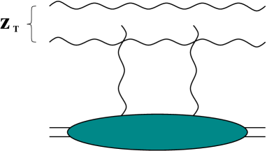
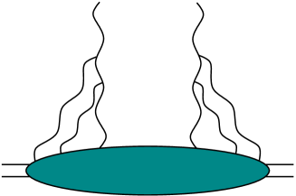
A	B

Figure 35: A. The definition of unintegrated gluon distribution relating it to the gluon dipole cross section from Eq. (205). The exchanged gluon lines can connect to either gluon in the dipole. B. The non-Abelian Weizsäcker-Williams gluon distribution obtained by calculating the correlator of two WW fields, given by Eq. (102).

Finally, we would like to point out the difference between the two unintegrated gluon distribution functions in Eqs. (205) and (102). We show the definitions of both distributions in Fig. 35. As was mentioned above, the WW gluon distribution from Eq. (102) is obtained by constructing a correlator of two WW gluon fields of Eq. (80). It is shown in Fig. 35B. It is this distribution which counts the number of gluon quanta and, in that sense, is the true unintegrated gluon distribution function. (The distribution from Eq. (102) should not be confused with the one we defined in Eq. (139) to connect the BK and GLR equations: the former is defined in terms of a gluon dipole, while the latter employs the quark dipole.) The gluon distribution from Eq. (205) was required to recast the gluon production cross section (194) in the $k_{T}$-factorization form of Eq. (207). However, its diagrammatic representation exists and is shown in Fig. 35A. There we consider the scattering amplitude of a gluon dipole on a nucleus. To define the gluon distribution from Eq. (205) one has to require that the interaction happens only via a two-gluon exchange, with some complicated gluon distribution in the nuclear wave function. It is not clear whether diagrammatic representation of the dipole-nucleus interaction from Fig. 35A is achievable in any known gauge. The bottom line is that it is rather puzzling that the $k_{T}$-factorization of Eq. (207) arises for the single gluon production cross section in $pA$, and it is also not clear why the unintegrated gluon distribution used in that formula should be given by Eq. (205), which the calculations lead to, instead of the physical gluon distribution of Eq. (102).

Eq. (205), along with Eqs. (206), allows one to generalize the gluon production cross section (194), which was originally derived for quark-nucleus scattering, to the case of proton-nucleus scattering. This could be done by using the gluon dipole–proton amplitude $n_{G}$ instead of the dipole-quark one from Eq. (203). However, the resulting two gluon distribution functions are different only by an overall prefactor, which is not important for our discussion below.

3.1.2 Nuclear Modification Factor: Low-$p_{T}$ Suppression

To analyze the properties of the particle production it is convenient to construct nuclear modification factor, which is defined experimentally as

$$R^{pA}(k_{T},y)\,\equiv\,\frac{\frac{dN^{pA}}{d^{2}k\ dy}}{N_{coll}\,\frac{dN^{pp}}{d^{2}k\ dy}},$$ (208)

where $N_{coll}$ is the number of proton-nucleon collisions in the $pA$ scattering process, $dN^{pA}/d^{2}kdy$ is the particle multiplicity in $pA$ scattering and $dN^{pp}/d^{2}kdy$ is the particle multiplicity in $pp$. $R^{pA}$ can be expressed in terms of particle production cross section as (for subtleties of this redefinition see [169])

$$R^{pA}(\underline{k},y)\,=\,\frac{\frac{d\sigma^{pA}}{d^{2}k\ dy}}{A\,\frac{d\sigma^{pp}}{d^{2}k\ dy}}.$$ (209)

In this and the following Sections we will study $R^{pA}$ given by the quasi-classical gluon production cross section derived above in Sect. 3.1.1. $R^{pA}$ for quark production, that will be derived later, can be constructed by analogy. To construct gluon $R^{pA}$ using Eq. (209) we will need the gluon production cross section (194), which we will use in the form given by Eq. (200), since it is more convenient for deriving various asymptotic regimes. Eq. (209) also requires us to know the gluon production in $pp$ collisions, which could be obtained by expanding $N_{G}$ from Eq. (103) to the lowest non-trivial order, corresponding to rescattering on a single nucleon in the nucleus, putting $A=1$ in it and using the resulting expression in Eq. (200). The result yields

$$A\,\frac{d\sigma^{pp}}{d^{2}k\ dy}\,=\,\frac{\alpha_{s}\,C_{F}}{\pi^{2}}\,\int d^{2}b\,\frac{Q_{s0}^{2}}{{\underline{k}}^{4}}\,\left(\ln\frac{{\underline{k}}^{2}}{4\,\Lambda^{2}}+2\,\gamma-1\right)\,\approx\,\frac{\alpha_{s}\,C_{F}}{\pi^{2}}\,\int d^{2}b\,\frac{Q_{s0}^{2}}{{\underline{k}}^{4}}\,\ln\frac{{\underline{k}}^{2}}{\Lambda^{2}}$$ (210)

with $\Lambda$ some infrared cutoff. In Eq. (210) we have included the factor of $A$ on the left hand side to make it ready to use in Eq. (209).

In this Section we are interested in the behavior of $R^{pA}({\underline{k}},y)$ at low values of the gluon transverse momentum $k_{T}$, namely for $k_{T}{{}_{\displaystyle{<}}\atop\displaystyle{\sim}}Q_{s0}$. Analyzing Eq. (200) we note that low $k_{T}{{}_{\displaystyle{<}}\atop\displaystyle{\sim}}Q_{s0}$ corresponds to dominance of large dipole sizes $z_{T}{{}_{\displaystyle{>}}\atop\displaystyle{\sim}}1/Q_{s0}$ in the integral. For $z_{T}{{}_{\displaystyle{>}}\atop\displaystyle{\sim}}1/Q_{s0}$ the cross section is likely to be black, and we can approximate $N_{G}$ in Eq. (200) by $N_{G}(\underline{z},\underline{b},0)\approx 1$. Integrating the resulting expression over $\underline{z}$ we obtain

$$\frac{d\sigma^{pA}}{d^{2}k\ dy}\,\approx\,\frac{\alpha_{s}\,C_{F}}{\pi^{2}}\,\int d^{2}b\,\frac{1}{{\underline{k}}^{2}},\hskip 28.45274ptk_{T}<Q_{s0}.$$ (211)

Before we proceed, let us point a very important property of the classical gluon production cross section (194). Eq. (210) in fact reflects a high-$k_{T}$ asymptotics of the gluon production cross section: at high-$k_{T}$ it scales as $\sim 1/k_{T}^{4}$, in agreement with the lowest order perturbative calculations [45, 28, 29, 30, 31, 46]. This result is badly infrared divergent, and demonstrates a problem of lowest order perturbative calculation of gluon production, shown in Fig. 5: if one wants to obtain the integral production cross section $d\sigma/dy$ from it, one would have to introduce an infrared cutoff $\Lambda$ for $k_{T}$-integration. The result would depend on the cutoff as $\sim 1/\Lambda^{2}$, making the resulting $d\sigma/dy$ very sensitive to the value of the cutoff and demonstrating that the lowest order cross section is dominated by non-perturbative infrared effects, which we do not know how to account for theoretically. On the other hand the full classical cross section of Eq. (194) is (almost) free of such problems. Eq. (211) describes the low-$k_{T}$ asymptotics of the cross section in Eq. (194). As one can see it leads to the cross section scaling as $\sim 1/k_{T}^{2}$. Thus, similar to the classical gluon distribution of Sect. 2.2.2 (see Fig. 17), the multiple rescattering effects regulate the infrared singularity, changing it from $\sim 1/k_{T}^{4}$ to $\sim 1/k_{T}^{2}$, and making the resulting cross section less infrared divergent. The residual infrared divergence $\sim 1/k_{T}^{2}$ is due to the fact that we have assumed that saturation behavior with multiple rescatterings takes place only in the nuclear wave function: there is no saturation in the proton wave function in the approach used here. The case of multiple rescatterings in both the target and the projectile is usually studied in the context of nucleus-nucleus ($AA$) collisions. There the residual $\sim 1/k_{T}^{2}$ divergence is regulated completely [43, 44, 41].

Using Eqs. (211) and (210) in Eq. (209) yields

$$R^{pA}(\underline{k},y)\,\approx\,\frac{k_{T}^{2}}{Q_{s0}^{2}\,\ln(k_{T}^{2}/\Lambda^{2})},\hskip 28.45274ptk_{T}<Q_{s0},$$ (212)

where, for simplicity, we assumed again that the nuclei are cylindrical in the beam ($z$) direction, such that the impact parameter integration over $\underline{b}$ in Eqs. (211) and (210) would give a trivial overall factor of the nuclear transverse area $S_{\perp}$, which cancels in $R^{pA}$. From Eq. (212) we see that [82, 64, 85, 62, 32, 86, 87, 88, 89]

$$R^{pA}(\underline{k},y)\,<\,1,\hskip 28.45274ptk_{T}<Q_{s0}.$$ (213)

Therefore we conclude that classical gluon production in $pA$ leads to suppression of low-$k_{T}$ gluons.

3.1.3 Nuclear Modification Factor: Cronin Effect

Our goal now is to study the nuclear modification factor $R^{pA}$ for high-$k_{T}$ particles with $k_{T}>Q_{s0}$. Starting with gluon production again we note that, in the quasi-classical case one can prove the following sum rule [62]

$$\int d^{2}k\,{\underline{k}}^{2}\,\frac{d\sigma^{pA}}{d^{2}k\ dy}\,=\,A\,\int d^{2}k\,{\underline{k}}^{2}\,\frac{d\sigma^{pp}}{d^{2}k\ dy},$$ (214)

which could be obtained from Eq. (200) using the fact that, for the quasi-classical amplitude (103) and the two-gluon exchange amplitude from Eq. (203) the following relation is true

$$\lim_{z_{T}\rightarrow 0}\left\{\left[\nabla^{2}_{z}\,N_{G}({\underline{z}},{\underline{b}},0)\right]-A^{1/3}\,\left[\nabla^{2}_{z}\,n_{G}({\underline{z}},{\underline{b}},0)\right]\right\}\,=\,0.$$ (215)

Eq. (215) and the sum rule of Eq. (214) are valid in the quasi-classical case of McLerran-Venugopalan model only. (When quantum small-$x$ evolution is included, Eq. (215) ceases to be valid.)

The sum rule (214) insures that if the quasi-classical gluon production cross section in $pA$ collisions is, in some region of $k_{T}$, smaller than $A$ times the gluon production cross section in $pp$ than there should be some other region of $k_{T}$ in which their roles are reversed. For $R^{pA}$ defined in Eq. (209) that means that if, in some region of $k_{T}$, it is less than $1$ there must be some other region of $k_{T}$ in which it is greater than $1$. Since in the previous section we have proven that $R^{pA}<1$ for $k_{T}<Q_{s0}$, the sum rule (214) demands that $R^{pA}>1$ for some region of $k_{T}$ in the $k_{T}>Q_{s0}$ interval. Enhancement of particle production in $pA$ collisions leading to $R^{pA}>1$ was originally observed by Cronin et al in [84] and is usually referred to as Cronin effect. Eqs. (214) and (213) prove that the cross section (194) leads to Cronin enhancement of produced gluons in $pA$ collisions.

Figure 36: The ratio $R^{pA}$ for gluons plotted as a function of $k_{T}/Q_{s0}$ in the quasi-classical McLerran-Venugopalan model as found in [32, 82, 64, 85, 62]. The cutoff is $\Lambda=0.2\,Q_{s}$.

To analyze the behavior of $R^{pA}$ for $k_{T}>Q_{s0}$ we follow the approach originally introduced in [35, 38] and find the first correction to the high-$k_{T}$ asymptotics of Eq. (194) given by Eq. (210). Expanding $N_{G}$ from Eq. (103) to the second non-trivial order, substituting the result in Eq. (200) and performing the integration over $\underline{z}$ we obtain [62]

$$\frac{d\sigma^{pA}}{d^{2}k\ dy}\,=\,\frac{\alpha_{s}\,C_{F}}{\pi^{2}}\,\int d^{2}b\,\frac{Q_{s0}^{2}}{{\underline{k}}^{4}}\,\left[\left(\ln\frac{{\underline{k}}^{2}}{4\,\Lambda^{2}}+2\,\gamma-1\right)+\right.$$

$$+\left.\frac{Q_{s0}^{2}}{4\,{\underline{k}}^{2}}\,\left(6\,\ln^{2}\frac{{\underline{k}}^{2}}{4\,\Lambda^{2}}-8\,(4-3\gamma)\,\ln\frac{{\underline{k}}^{2}}{4\,\Lambda^{2}}+29+24\,\gamma^{2}-64\,\gamma\right)+\ldots\right],\hskip 28.45274ptk_{T}\rightarrow\infty.$$ (216)

Substituting Eq. (216) along with Eq. (210) into Eq. (209) and keeping only the leading logarithmic ($\ln(k_{T}^{2}/\Lambda^{2})$) terms in the parentheses of Eq. (216) yields for a cylindrical nucleus [62]

$$R^{pA}(k_{T})\,=\,1+\frac{3}{2}\,\frac{Q_{s0}^{2}}{{\underline{k}}^{2}}\,\ln\frac{k_{T}^{2}}{\Lambda^{2}}+\ldots,\hskip 28.45274ptk_{T}\rightarrow\infty.$$ (217)

Eq. (217) indicates that $R^{pA}$ approaches $1$ from above at high $k_{T}$, which is typical of Cronin enhancement [84]. We therefore conclude that in the framework of the quasi-classical approximation employed in arriving at Eq. (194) the ratio $R^{pA}$ is less than $1$ at small $k_{T}{{}_{\displaystyle{<}}\atop\displaystyle{\sim}}Q_{s0}$ and displays Cronin enhancement at high $k_{T}{{}_{\displaystyle{>}}\atop\displaystyle{\sim}}Q_{s0}$. This conclusion has been reached in [82, 64, 85, 62, 32, 86, 87, 88, 89].

To summarize let us note that, if one neglects the logarithms in the exponents of Eq. (194) as a slowly varying functions of transverse separations, writing for instance $\underline{x}^{2}\ln(1/x_{T}\Lambda)\approx\underline{x}^{2}$, it would become possible to perform the $\underline{x}$ and $\underline{y}$ integrations in Eq. (194) exactly, obtaining [32, 62]

$$\frac{d\sigma^{pA}}{d^{2}k\ dy}\,=\,\frac{\alpha_{s}\,C_{F}}{\pi^{2}}\,\int d^{2}b\,\left\{-\frac{1}{{\underline{k}}^{2}}+\frac{2}{{\underline{k}}^{2}}\,e^{-{\underline{k}}^{2}/Q_{s0}^{2}}+\frac{1}{Q_{s0}^{2}}\,e^{-{\underline{k}}^{2}/Q_{s0}^{2}}\,\left[\ln\frac{Q_{s0}^{4}}{4\,\Lambda^{2}{\underline{k}}^{2}}+\mbox{Ei}\left(\frac{{\underline{k}}^{2}}{Q_{s0}^{2}}\right)\right]\right\},$$ (218)

where $\mathrm{Ei}(x)$ is the exponential integral. Expanding Eq. (218) would give the gluon production cross section in $pp$, which can be obtained from Eq. (210) by dropping $\ln(k_{T}^{2}/\Lambda^{2})$ in it. The nuclear modification factor resulting from Eq. (218) is [62]

$$R^{pA}(k_{T})\,=\,\frac{{\underline{k}}^{4}}{Q_{s0}^{2}}\,\left\{-\frac{1}{{\underline{k}}^{2}}+\frac{2}{{\underline{k}}^{2}}\,e^{-{\underline{k}}^{2}/Q_{s0}^{2}}+\frac{1}{Q_{s0}^{2}}\,e^{-{\underline{k}}^{2}/Q_{s0}^{2}}\,\left[\ln\frac{Q_{s0}^{4}}{4\,\Lambda^{2}{\underline{k}}^{2}}+\mbox{Ei}\left(\frac{{\underline{k}}^{2}}{Q_{s0}^{2}}\right)\right]\right\}.$$ (219)

The ratio $R^{pA}(k_{T})$ is plotted in Fig. 36 for $\Lambda=0.2\ Q_{s0}$. It clearly exhibits an enhancement at high-$k_{T}$ [82, 64, 85, 62, 32, 86, 87, 88, 89] typical of Cronin effect [84]. The height and position of Cronin maximum are increasing functions of $Q_{s}$, and, therefore, of collision centrality [64, 62].

3.2 Gluon Production Including Quantum Evolution

Here we are going to show how to include the effects of quantum BK evolution equation from Sect. 2.3 into the gluon production cross section derived in Sect. 3.1. We will then analyze the impact of small-$x$ evolution on the nuclear modification factor $R^{pA}$, demonstrating that it eliminates Cronin enhancement leading to suppression of gluon production at all transverse momenta $k_{T}$.

3.2.1 Gluon Production Cross Section

Starting with the gluon production cross section, let us first solve the problem of gluon production in deep inelastic scattering (DIS) instead of $pA$ collisions. The advantage of DIS is that we know explicitly how to include the non-linear small-$x$ evolution into the dipole wave function, as shown in Fig. 24 and given by Eq. (135). The answer we will obtain this way would be easy to generalize to the case of $pA$ collisions.

Figure 37: Gluon production in DIS in the quasi-classical approximation. The produced gluon may be emitted either off the quark or off the antiquark lines both in the amplitude and in the complex conjugate amplitude. Only one connection is shown.

The problem of including the effects of BK evolution into the quasi-classical gluon production cross section from Eq. (194) could be thought of as producing one of the gluons in the non-linear cascade of Fig. 24. However, the cascade we needed for calculation of the total DIS cross section is somewhat different from what we need now for the inclusive cross section. The difference is in the fact that the cascade of Fig. 24 develops from early times, with light cone time $\tau\equiv x^{-}=-\infty$, till the interaction with the nucleus at $\tau=0$. Since Fig. 24 represents the forward scattering amplitude, the evolution of the cascade after the interaction, during the times between $\tau=0$ and $\tau=+\infty$, is restricted to one simple case when the system returns back to the initial state and nothing is produced. This is the definition of the forward amplitude and this is all we need to calculate the total cross section. To calculate the inclusive cross section we need to square the production amplitude, as was shown in, for instance, Fig. 31, for the quasi-classical case. There, already in the amplitude, we had to include the diagrams where the incoming proton would “cascade”, generating a gluon both before the interaction in the time interval $\tau=-\infty\ldots 0$ and after the interaction, at $\tau=0\ldots+\infty$. Therefore, to construct a gluon cascade making sure that we always have the gluon we are trying to produce in the final state, we have to include gluon emissions bringing in logarithms of energy both at $\tau=-\infty\ldots 0$ and $\tau=0\ldots+\infty$ in the amplitude and in its complex conjugate.

To do that let us first generalize the quasi-classical expression from Eq. (194) to the case of DIS. The relevant diagrams are shown in Fig. 37. They are similar to the case of quark-nucleus scattering pictured in Fig. 31. The major difference is that now we have an incoming $q\bar{q}$ dipole instead of just a single quark. The produced gluon can, therefore, be emitted off of either quark and anti-quark lines on both sides of the cut. In Fig. 37 we show only one particular way of emitting the gluon. Diagrams A and B in Fig. 37 correspond to diagrams A and B in Fig. 31. Another difference now is the diagram in Fig. 37C, which used to cancel through real-virtual cancellations in quark–nucleus scattering case and was not even shown in Fig. 31, is now non-zero and has to be included. This is due to the fact that moving a $t$-channel exchanged gluon across the cut in Fig. 37C would change the color factor of the diagram, thus preventing the cancellation. Adding all the diagrams in Fig. 37, and summing over all possible emissions of the gluon off the quark and anti-quark lines, we write for the gluon production cross section in the dipole-nucleus scattering [132, 34]

$$\frac{d{\hat{\sigma}}^{q{\bar{q}}A}}{d^{2}k\,dy\,d^{2}B}({\underline{x}}_{01})\,=\,\frac{\alpha_{s}C_{F}}{\pi^{2}}\,\frac{1}{(2\pi)^{2}}\,\int\,d^{2}z_{1}\,d^{2}z_{2}\,e^{-i{\underline{k}}\cdot({\underline{z}}_{1}-{\underline{z}}_{2})}\,\sum_{i,j=0}^{1}(-1)^{i+j}\frac{{\underline{z}}_{1}-{\underline{x}}_{i}}{|{\underline{z}}_{1}-{\underline{x}}_{i}|^{2}}\cdot\frac{{\underline{z}}_{2}-{\underline{x}}_{j}}{|{\underline{z}}_{2}-{\underline{x}}_{j}|^{2}}$$

$$\times\bigg{[}N_{G}\left({\underline{z}}_{1}-{\underline{x}}_{j},\frac{1}{2}({\underline{z}}_{1}+{\underline{x}}_{j}),0\right)+N_{G}\left({\underline{z}}_{2}-{\underline{x}}_{i},\frac{1}{2}({\underline{z}}_{2}+{\underline{x}}_{i}),0\right)-N_{G}\left({\underline{z}}_{1}-{\underline{z}}_{2},\frac{1}{2}({\underline{z}}_{1}+{\underline{z}}_{2}),0\right)$$

$$-N_{G}\left({\underline{x}}_{i}-{\underline{x}}_{j},\frac{1}{2}({\underline{x}}_{i}+{\underline{x}}_{j}),0\right)\bigg{]},$$ (220)

where, just like in Sect. 2.3.2, the quark and the anti-quark have transverse coordinates ${\underline{x}}_{0}$ and ${\underline{x}}_{1}$ correspondingly. The rest of the notation of Eq. (3.2.1) is explained in Fig. 37. $N_{G}$ in Eq. (3.2.1) is taken from Eq. (103), and now we put the correct impact parameters for all the dipoles.

To include the effects of small-$x$ evolution we should add to the graphs in Fig. 37 the diagrams with more gluon emissions before and after the interaction. Let us denote the rapidity of the target nucleus as $0$ and the rapidity of the incoming $q\bar{q}$ dipole as $Y$. The produced gluon would have rapidity $y$. Following [34] we will divide all possible extra gluon emission into two categories: the gluons can have rapidities larger (harder) or smaller (softer) than $y$.

Figure 38: Emission of a harder gluon in the dipole evolution, as considered in [34]. Gluons are denoted by double lines in the large $N_{c}$ limit. The produced gluon is marked by a cross. Dashed lines comprise multiple rescatterings with the target from Fig. 11, which are instantaneous on the time scale of the dipole evolution.

First we analyze the emissions of harder gluons. Some of the relevant diagrams are shown in Fig. 38. Since we are trying to apply quantum evolution from Mueller’s dipole model [19, 20, 21] we are again working in the large-$N_{c}$ limit. Similar to Fig. 25 the gluons are denoted by double lines which do not connect to any particular quark or anti-quark lines in the dipole in which a particular gluon is emitted: this denotes summation over both connections on both sides of the cut. In Fig. 38 the gluon $3$ is the one that we measure in the final state, the gluon $2$ is a harder gluon emitted before gluon $3$. Solid vertical lines in Fig. 38 denote the $\tau=+\infty$ final state, while the dashed vertical lines denote the multiple rescattering interactions with the target from Fig. 11 taking place at $\tau=0$ on both sides of the cut.

In Sect. 2.3.2 we have demonstrated that successive emissions of progressively softer gluons before the interaction (for $\tau=-\infty\ldots 0$) give the leading logarithmic contribution, in the sense of giving a factor of $Y$ for each factor of $\alpha_{s}$ resumming the parameter $\alpha_{s}Y$, as is accomplished by Eq. (135). Interestingly enough, this ordering has to be reversed for emissions after the interaction (for $\tau=0\ldots+\infty$): to obtain the leading logarithmic contribution ($\alpha_{s}Y$), softer gluons have to be emitted before harder ones at $\tau=0\ldots+\infty$ [34]. More details on how this happens could be found in [34]. Indeed, if emission of a harder gluon happened after the emission of the softer one, the harder gluon can not be emitted off the softer one: it is emitted by hard quark lines of the original dipole [34]. Since the diagrams E–I in Fig. 38 violate such inverse ordering, they can be discarded. Only the diagrams A–D in Fig. 38 contribute. Those are real contributions to the dipole evolution leading to production of the dipole in which gluon $3$ was emitted. Note that all of these surviving diagrams have early time ($\tau=-\infty\ldots 0$) emissions only: they correspond to standard dipole evolution of Fig. 24. A similar analysis shows that out of the rest of the diagrams with possible emissions of gluon $2$, the ones that bring in leading logarithmic contribution are the ones which give virtual corrections to the dipole evolution at light cone times $\tau=-\infty\ldots 0$ [34]. Emissions of other harder gluons do not change the conclusions: the surviving diagrams are the ones which contribute to dipole evolution leading to production of the dipole in which gluon $3$ was emitted. Such evolution is described by the quantity $n_{1}({\underline{x}}_{01},{\underline{x}}_{0^{\prime}1^{\prime}},{\underline{B}}-{\underline{b}},Y-y)$, originally introduced in [19, 20], which has the meaning of the number of dipoles of size ${\underline{x}}_{0^{\prime}1^{\prime}}$ at rapidity $y$ and impact parameter $\underline{b}$ generated by evolution from the original dipole ${\underline{x}}_{01}$ having rapidity $Y$ and impact parameter $\underline{B}$. This quantity obeys the dipole model analogue of the BFKL equation [27], which is just the linear part of Eq. (135) [19, 20]

$$\frac{\partial n_{1}({\underline{x}}_{01},{\underline{x}}_{0^{\prime}1^{\prime}},{\underline{b}},y)}{\partial y}\,=\,\frac{\alpha_{s}\,N_{c}}{2\,\pi^{2}}\,\int d^{2}x_{2}\,\frac{x_{01}^{2}}{x_{20}^{2}\,x_{21}^{2}}\,\bigg{[}n_{1}({\underline{x}}_{02},{\underline{x}}_{0^{\prime}1^{\prime}},{\underline{b}}+\frac{1}{2}\,{\underline{x}}_{21},y)+n_{1}({\underline{x}}_{12},{\underline{x}}_{0^{\prime}1^{\prime}},{\underline{b}}+\frac{1}{2}\,{\underline{x}}_{20},y)$$

$$-n_{1}({\underline{x}}_{01},{\underline{x}}_{0^{\prime}1^{\prime}},{\underline{b}},y)\bigg{]}$$ (221)

with the initial condition

$$n_{1}({\underline{x}}_{01},{\underline{x}}_{0^{\prime}1^{\prime}},{\underline{b}},y=0)\,=\,\delta({\underline{x}}_{01}-{\underline{x}}_{0^{\prime}1^{\prime}})\,\delta({\underline{b}}).$$ (222)

The inclusion of the effects of harder gluons in Eq. (3.2.1) is then accomplished by replacing the cross section in Eq. (3.2.1) by [34]

$$\frac{d{\hat{\sigma}}^{q{\bar{q}}A}}{d^{2}k\,dy\,d^{2}B}({\underline{x}}_{01})\rightarrow\int d^{2}b\,d^{2}x_{0^{\prime}1^{\prime}}\ n_{1}({\underline{x}}_{01},{\underline{x}}_{0^{\prime}1^{\prime}},{\underline{B}}-{\underline{b}},Y-y)\ \frac{d{\hat{\sigma}}^{q{\bar{q}}A}}{d^{2}k\,dy\,d^{2}b}({\underline{x}}_{0^{\prime}1^{\prime}}).$$ (223)

Now we have to resum emissions of softer gluons having rapidity less than the rapidity of the produced gluon $y$.

Figure 39: Diagrams including one softer gluon produced after the emission of the measured gluon [34].

Such emissions are demonstrated in Fig. 39, where now the gluon $2$ is softer than the gluon $3$. Fig. 39 only has emissions where gluon $2$ interacts with gluon $3$ and with either the quark or the anti-quark lines in the dipole. As was shown in [34], such diagrams cancel pairwise via real-virtual cancellations:

$$A+D=0,\hskip 14.22636ptB+C=0,\hskip 14.22636ptF+G=0,\hskip 14.22636ptE+H=0.$$ (224)

The diagrams where gluon $2$ connects only to the quark and the anti-quark lines cancel analogously [34]. The only remaining diagrams are where the gluon $2$ is emitted and reabsorbed by gluon $3$ only. Using the crossing symmetry [167] we reflect the line of gluon $3$ into the complex conjugate amplitude (denoted by $3^{\prime}$) with respect to the cut, obtaining a gluon dipole in the amplitude, just like we did in Sect. 3.1.1 to obtain Eq. (194). Then it becomes manifest that emission of gluon $2$ can be thought of as one iteration of dipole evolution in the gluon dipole $33^{\prime}$. Successive emissions of even softer gluon would not modify this conclusion. Therefore, to include the effects of softer gluon emissions in Eq. (3.2.1) we have to replace [34]

$$N_{G}({\underline{x}},{\underline{b}},0)\rightarrow N_{G}({\underline{x}},{\underline{b}},y)$$ (225)

on its right hand side, where now $N_{G}({\underline{x}},{\underline{b}},y)$ is the amplitude of a gluon dipole interacting with the nucleus including the small-$x$ evolution of Eq. (135). In the large-$N_{c}$ limit $N_{G}$ can be expressed in terms of the quark dipole amplitude $N$ from Eq. (135) as

$$N_{G}({\underline{x}},{\underline{b}},y)\,=\,2\,N({\underline{x}},{\underline{b}},y)-N^{2}({\underline{x}},{\underline{b}},y),$$ (226)

since a gluon dipole in the large-$N_{c}$ limit can be thought of as a pair of quark dipoles, with either one of them or both quark dipoles interacting.

Combining the prescriptions for including quantum evolution for hard (223) and soft (225) emissions we obtain the following expression for inclusive gluon production cross section in DIS [34]

$$\frac{d\sigma^{q{\bar{q}}A}}{d^{2}k\ dy\,d^{2}B}({\underline{x}}_{01})\ =\ \int\,d^{2}x_{0^{\prime}1^{\prime}}\,n_{1}({\underline{x}}_{01},{\underline{x}}_{0^{\prime}1^{\prime}},{\underline{B}}-{\underline{b}},Y-y)\,\frac{\alpha_{s}C_{F}}{\pi^{2}}\,\frac{1}{(2\pi)^{2}}\,d^{2}b$$

$$\times\,d^{2}z_{1}\,d^{2}z_{2}\,e^{-i{\underline{k}}\cdot({\underline{z}}_{1}-{\underline{z}}_{2})}\,\sum_{i,j=0^{\prime}}^{1^{\prime}}(-1)^{i+j}\,\frac{{\underline{z}}_{1}-{\underline{x}}_{i}}{|{\underline{z}}_{1}-{\underline{x}}_{i}|^{2}}\cdot\frac{{\underline{z}}_{2}-{\underline{x}}_{j}}{|{\underline{z}}_{2}-{\underline{x}}_{j}|^{2}}\left[N_{G}\left({\underline{z}}_{1}-{\underline{x}}_{j},\frac{1}{2}({\underline{z}}_{1}+{\underline{x}}_{j}),y\right)+\right.$$

$$+\left.N_{G}\left({\underline{z}}_{2}-{\underline{x}}_{i},\frac{1}{2}({\underline{z}}_{2}+{\underline{x}}_{i}),y\right)-N_{G}\left({\underline{z}}_{1}-{\underline{z}}_{2},\frac{1}{2}({\underline{z}}_{1}+{\underline{z}}_{2}),y\right)-N_{G}\left({\underline{x}}_{i}-{\underline{x}}_{j},\frac{1}{2}({\underline{x}}_{i}+{\underline{x}}_{j}),y\right)\right].$$ (227)

Eq. (227) provides us with the single inclusive gluon production cross section for scattering of the quark–anti-quark dipole $01$ on the target nucleus, which includes all multiple rescatterings (powers of $\alpha_{s}^{2}A^{1/3}$) and small-$x$ evolution corrections (powers of $\alpha_{s}Y$ and $\alpha_{s}y$) [34].

Figure 40: Interpretation of the inclusive gluon production in $pA$ collisions from Eq. (227) in terms of fan diagrams.

If one associates Eq. (135) with summation of fan diagrams from Fig. 9, than one can represent Eq. (227) in the way shown in Fig. 40. There the interaction between the quark–anti-quark dipole and the target is mediated by exchange of fan diagrams, where we trigger on one of the produced gluons, which is denoted by the cross. The part of the diagram between the produced gluon and the projectile dipole is described in Eq. (227) by the quantity $n_{1}({\underline{x}}_{01},{\underline{x}}_{0^{\prime}1^{\prime}},{\underline{B}}-{\underline{b}},Y-y)$, which satisfies linear BFKL evolution equation (221). In terms of ladder and fan diagrams, that corresponds to having just a single ladder exchange between the dipole and the produced gluon, as shown in Fig. 40. In principle one could draw gluon production diagrams where the ladder between the dipole and produced gluon would split into several ladders interacting with the target. However, Eq. (227) implies that such graphs cancel. The same cancellation is expected if one applies AGK cutting rules to QCD diagrams [170, 171, 90]. It is intriguing to see AGK rules work in perturbative QCD in the framework of the dipole model. They have also been found to work previously for single diffractive cross sections in DIS calculated in the dipole model approach [131]. However, the AGK rules appear to break down in QCD for inclusive two-particle production cross sections [103, 36, 104].

In the limit of a very large target nucleus the momentum transfer to the nucleus is cut off by inverse nuclear radius and is very small. We can therefore take the scattering amplitudes $N_{G}$ in Eq. (227) at $t=0$, which in coordinate space is equivalent to neglecting (factoring out) the impact parameter dependence since the shifts in impact parameter in Eq. (227) are small compared to the nuclear radius [166, 172]. We, therefore, put all the impact parameters in $N_{G}$’s of Eq. (227) to be equal to $\underline{b}$. Repeating the steps outlined at the end of Sect. 3.1.1 we arrive at [34]

$$\frac{d\sigma^{q{\bar{q}}A}}{d^{2}k\ dy}\,=\,\frac{2\,\alpha_{s}}{C_{F}}\,\frac{1}{{\underline{k}}^{2}}\,\int d^{2}q\,\phi_{q\bar{q}}({\underline{q}},Y-y)\,\phi_{A}({\underline{k}}-{\underline{q}},y)$$ (228)

with $\phi_{A}({\underline{k}}-{\underline{q}},y)$ given by Eq. (205) and the unintegrated gluon distribution in the dipole given by [34, 103]

$$\phi_{q\bar{q}}({\underline{q}},y)\,=\,\frac{2\,\alpha_{s}\,C_{F}}{\pi}\,\int d^{2}b\,d^{2}x_{0^{\prime}1^{\prime}}\,e^{-i{\underline{q}}\cdot{\underline{x}}_{0^{\prime}1^{\prime}}}\,\frac{1}{\nabla^{2}_{x_{0^{\prime}1^{\prime}}}}\,n_{1}({\underline{x}}_{01},{\underline{x}}_{0^{\prime}1^{\prime}},{\underline{b}},y).$$ (229)

Interestingly enough, as we see from Eq. (228), the small-$x$ evolution does not lead to break-down of the $k_{T}$-factorization formula (207)! In fact, Eq. (228), with the gluon distribution functions given by Eq. (229) and by Eq. (205), only with twice the quark dipole amplitude $2\,N$ instead of $N_{G}$, was postulated as the answer for inclusive gluon production cross section by Braun in [90] using $k_{T}$-factorization approach. Still, Eq. (228), obtained in [34], differs from the result of [90] by the difference in $N_{G}$ and $2\,N$ (see Eq. (226)), which in the standard pomeron language appears to corresponds to emission of the produced gluon from the triple pomeron vertex [91]. This difference may become numerically significant for low transverse momenta of the produced gluon, as was shown in [91].

Now generalization to the case of $pA$ becomes manifest: we have to replace the unintegrated gluon distribution function of a dipole, $\phi_{q\bar{q}}({\underline{q}},y)$, by the one for the proton, $\phi_{p}({\underline{q}},y)$, given by Eq. (206) with $n_{G}$ satisfying the linear part of Eq. (135)

$$\frac{\partial n_{G}({\underline{x}}_{01},{\underline{b}},y)}{\partial y}\,=\,\frac{\alpha_{s}\,N_{c}}{2\,\pi^{2}}\,\int d^{2}x_{2}\,\frac{x_{01}^{2}}{x_{20}^{2}\,x_{21}^{2}}\,\bigg{[}n_{G}({\underline{x}}_{02},{\underline{b}}+\frac{1}{2}\,{\underline{x}}_{21},y)+n_{G}({\underline{x}}_{12},{\underline{b}}+\frac{1}{2}\,{\underline{x}}_{20},y)-n_{G}({\underline{x}}_{01},{\underline{b}},y)\bigg{]}$$ (230)

with Eq. (203) as the initial condition. To summarize, the inclusive cross section from Eq. (228) becomes in the case of $pA$

$$\frac{d\sigma^{pA}}{d^{2}k\ dy}\,=\,\frac{2\,\alpha_{s}}{C_{F}}\,\frac{1}{{\underline{k}}^{2}}\,\int d^{2}q\,\phi_{p}({\underline{q}},Y-y)\,\phi_{A}({\underline{k}}-{\underline{q}},y)$$ (231)

with the unintegrated gluon distributions given by Eqs. (205) and (206) with the dipole cross sections evolved with Eqs. (135) and (230) correspondingly.

Indeed Eq. (228) was derived in the large-$N_{c}$ limit. It appear hard (though maybe not impossible) to generalize the large-$N_{c}$ dipole model to the case of projectile proton: therefore, we can not prove the suggested generalization to the proton case. However, this generalization is probably a good approximation of the exact answer for the following reasons. We showed that $k_{T}$-factorization works in the quasi-classical case to all orders in $N_{c}$ (see Eq. (207)). We have also shown that it survives evolution corrections (Eq. (228)). Therefore, factorization formula (231), which expresses the production cross section in terms of gluon dipole amplitudes scattering on the projectile and on the target, is probably valid in the general case of including small-$x$ evolution beyond the large-$N_{c}$ limit. The results of numerical solution of the full JIMWLK evolution equation for the dipole amplitude were shown to be amazingly close to the solution of BK equation [18]. The linear BFKL evolution analogue in the dipole model [19] gives the same value for the pomeron intercept as the exact BFKL equation [27]. Therefore, it is probably safe to use Eq. (231) for the gluon production in $pA$, even though strictly speaking it should work only for the case when the proton is approximated by a di-quark. Both pA and DIS processes are considered here as scatterings of an unsaturated projectile (proton or $q\bar{q}$ pair) on a saturated target (nucleus), and, therefore, gluon production cross sections for them should be similar. Therefore, we will use Eq. (231) for the analysis outlined below of the gluon production in $pA$.

3.2.2 Nuclear Modification Factor: Double Logarithmic Region

Let us now analyze what happens to nuclear modification factor (209) when quantum evolution is included. To do that, we use Eqs. (205) and (206) to rewrite Eq. (231) as

$$\frac{d\sigma^{pA}}{d^{2}k\ dy}\,=\,\frac{C_{F}}{\alpha_{s}\,\pi\,(2\pi)^{3}}\,\frac{1}{{\underline{k}}^{2}}\,\int d^{2}B\,d^{2}b\,d^{2}z\,\nabla^{2}_{z}\,n_{G}({\underline{z}},{\underline{B}}-{\underline{b}},Y-y)\,e^{-i{\underline{k}}\cdot{\underline{z}}}\,\nabla^{2}_{z}\,N_{G}({\underline{z}},{\underline{b}},y).$$ (232)

For simplicity, let us neglect the impact parameter dependence of $N_{G}$ throughout the nucleus and of $n_{G}$ over the transverse area of the proton. Suppressing the impact parameter dependence in the arguments of $N_{G}$ and $n_{G}$ in Eq. (232) we rewrite it as

$$\frac{d\sigma^{pA}}{d^{2}k\ dy}\,=\,\frac{C_{F}}{\alpha_{s}\,\pi\,(2\pi)^{3}}\,\frac{S_{p}\,S_{A}}{{\underline{k}}^{2}}\,\int d^{2}z\,\nabla^{2}_{z}\,n_{G}({\underline{z}},Y-y)\,e^{-i{\underline{k}}\cdot{\underline{z}}}\,\nabla^{2}_{z}\,N_{G}({\underline{z}},y),$$ (233)

with $S_{A}$ and $S_{p}$ the cross sectional areas of the nucleus and the proton correspondingly. In this Section, and in the one below, we will be interested in gluon production with large $k_{T}{{}_{\displaystyle{>}}\atop\displaystyle{\sim}}Q_{s}(y)$, such that nonlinear effects could be neglected in $N_{G}$. Outside of the saturation region we write, similar to Eq. (148),

$$N_{G}(z_{T},y)\,=\,\int_{-\infty}^{\infty}d\nu\ e^{2\,\overline{\alpha}_{s}\,\chi(0,\nu)\,y}\,(z_{T}Q_{s0})^{1+2\,i\,\nu}\,C_{\nu}^{A},$$ (234)

where $C_{\nu}^{A}$ is determined by the initial condition of Eq. (103). Similarly, for $n_{G}$ one writes the general $\underline{b}$-independent solution of Eq. (230) as

$$n_{G}(z_{T},y)\,=\,\int_{-\infty}^{\infty}d\nu\ e^{2\,\overline{\alpha}_{s}\,\chi(0,\nu)\,y}\,(z_{T}\Lambda_{p})^{1+2\,i\,\nu}\,C_{\nu}^{p},$$ (235)

where, to satisfy the initial condition given by Eq. (203),

$$C_{\nu}^{p}\,=\,\frac{1}{4\,\pi\,(1-2\,i\,\nu)^{2}}$$ (236)

and

$$\Lambda^{2}_{p}\,=\,4\,\pi\,\alpha_{s}^{2}\,\frac{1}{S_{p}}.$$ (237)

Substituting Eqs. (234) and (235) into Eq. (233) and integrating over $\underline{z}$ yields

$$\frac{d\sigma^{pA}}{d^{2}k\ dy}\,=\,\frac{C_{F}\,S_{p}\,S_{A}}{\alpha_{s}\,(2\pi)^{3}}\,\int_{-\infty}^{\infty}d\nu\,d\nu^{\prime}\,C_{\nu}^{A}\,C_{\nu^{\prime}}^{p}\,(1+2i\nu)^{2}\,(1+2i\nu^{\prime})^{2}\,2^{2i(\nu+\nu^{\prime})}\,\frac{\Gamma[i(\nu+\nu^{\prime})]}{\Gamma[1-i(\nu+\nu^{\prime})]}$$

$$\times\,\left(\frac{Q_{s0}}{k_{T}}\right)^{1+2i\nu}\,\left(\frac{\Lambda_{p}}{k_{T}}\right)^{1+2i\nu^{\prime}}\,e^{2\,\overline{\alpha}_{s}\,\chi(0,\nu)\,y+2\,\overline{\alpha}_{s}\,\chi(0,\nu^{\prime})\,(Y-y)}$$ (238)

with $\overline{\alpha}_{s}$ given by Eq. (147).

In this Section we are interested in the double logarithmic region (DLA) where $k_{T}{{}_{\displaystyle{>}}\atop\displaystyle{\sim}}k_{\rm geom}\gg Q_{s}(y)$. Evaluating the $\nu$ and $\nu^{\prime}$ integrals in Eq. (238) in the stationary phase approximation around the saddle point from Eq. (154) with $\chi(0,\nu)$ (and $\chi(0,\nu^{\prime})$) given by Eq. (153) we obtain [161]

$$\frac{d\sigma^{pA}}{d^{2}k\ dy}\bigg{|}_{DLA}\,\approx\,\frac{C_{F}\,S_{p}\,S_{A}}{\alpha_{s}\,(2\pi)^{4}}\,\frac{Q_{s0}^{2}\,\Lambda_{p}^{2}}{{\underline{k}}^{4}}\,\frac{1}{2\,\overline{\alpha}_{s}}\,\left[\frac{\ln\frac{k_{T}}{Q_{s0}}\,\ln\frac{k_{T}}{\Lambda_{p}}}{y^{3}\,(Y-y)^{3}}\right]^{1/4}\,\left(\sqrt{\frac{y}{\ln\frac{k_{T}}{Q_{s0}}}}+\sqrt{\frac{Y-y}{\ln\frac{k_{T}}{\Lambda_{p}}}}\right)$$

$$\times\exp\left(2\sqrt{2\,\overline{\alpha}_{s}\,y\,\ln\frac{k_{T}}{Q_{s0}}}+2\sqrt{2\,\overline{\alpha}_{s}\,(Y-y)\,\ln\frac{k_{T}}{\Lambda_{p}}}\ \right).$$ (239)

In arriving at Eq. (239) we made use of Eq. (236), and have also used the fact that near the saddle point of Eq. (154) $C_{\nu}^{A}$ is approximately given by Eq. (236) as well [62].

To calculate $R^{pa}$ we also need the gluon production cross section in $pp$ collisions in the same kinematic DLA region, which can be obtained from Eq. (239) by replacing $S_{A}\rightarrow S_{p}$ and $Q_{s0}\rightarrow\Lambda_{p}$ in it [62]

$$\frac{d\sigma^{pp}}{d^{2}k\ dy}\bigg{|}_{DLA}\,\approx\,\frac{C_{F}\,S_{p}^{2}}{\alpha_{s}\,(2\pi)^{4}}\ \frac{\Lambda_{p}^{4}}{{\underline{k}}^{4}}\,\frac{1}{2\,\overline{\alpha}_{s}}\,\frac{\sqrt{y}+\sqrt{Y-y}}{y^{3/4}\,(Y-y)^{3/4}}\,\exp\left[2\sqrt{2\,\overline{\alpha}_{s}\,\ln\frac{k_{T}}{\Lambda_{p}}}\left(\sqrt{y}+\sqrt{Y-y}\right)\right].$$ (240)

Substituting Eqs. (239) and (240) in Eq. (209) and remembering that $S_{A}=A^{2/3}S_{p}$ and $Q_{s0}^{2}=A^{1/3}\Lambda_{p}^{2}$ yields

$$R^{pA}(k_{T},y)\bigg{|}_{k_{T}\gg Q_{s}}\,=\,\frac{\left(\ln\frac{k_{T}}{Q_{s0}}\,\ln\frac{k_{T}}{\Lambda_{p}}\right)^{1/4}}{\sqrt{y}+\sqrt{Y-y}}\,\left(\sqrt{\frac{y}{\ln\frac{k_{T}}{Q_{s0}}}}+\sqrt{\frac{Y-y}{\ln\frac{k_{T}}{\Lambda_{p}}}}\right)$$

$$\times\,\exp\left[2\sqrt{2\,\overline{\alpha}_{s}\,y}\left(\sqrt{\ln\frac{k_{T}}{Q_{s0}}}-\sqrt{\ln\frac{k_{T}}{\Lambda_{p}}}\right)\right].$$ (241)

The behavior of $R^{pA}(k_{T},y)$ from Eq. (241) at high $y$ is dominated by the exponent in it [62]

$$R^{pA}(k_{T},y)\bigg{|}_{k_{T}\gg Q_{s}}\,\approx\,\exp\left[2\sqrt{2\,\overline{\alpha}_{s}\,y}\left(\sqrt{\ln\frac{k_{T}}{Q_{s0}}}-\sqrt{\ln\frac{k_{T}}{\Lambda_{p}}}\right)\right]\,<\,1.$$ (242)

Since $Q_{s0}\gg\Lambda_{p}$, the exponent in Eq. (242) becomes less than $1$, driving $R^{pA}(k_{T},y)$ below one as well [62]. We therefore conclude that in the DLA region with $k_{T}{{}_{\displaystyle{>}}\atop\displaystyle{\sim}}k_{\rm geom}$, the nuclear modification factor becomes smaller than $1$ due to quantum evolution. This indicates suppression of gluon production due to quantum evolution. A suppression of $R^{pA}$ by small-$x$ evolution effects was originally suggested in [61], though the authors of [61] analyzed particle (gluon) production only in the geometric scaling region $k_{T}{{}_{\displaystyle{<}}\atop\displaystyle{\sim}}k_{\rm geom}$, which is what we are going to do now.

3.2.3 Nuclear Modification Factor: Extended Geometric Scaling Region

In the extended geometric scaling region, $Q_{s}(Y)<k_{T}{{}_{\displaystyle{<}}\atop\displaystyle{\sim}}k_{\rm geom}$, multiple rescatterings are still unimportant and Eq. (238) from the previous Section still applies. To obtain the leading behavior of Eq. (238) in the geometric scaling region we will evaluate the $\nu$-integral in it by simply replacing $\nu$ with $\nu_{0}$ from Eq. (163) in the integrand, as it was done in obtaining Eq. (180). We obtain

$$\frac{d\sigma^{pA}}{d^{2}k\ dy}\,=\,\frac{C_{F}\,S_{p}\,S_{A}}{\alpha_{s}\,(2\pi)^{3}}\ C_{\nu_{0}}^{A}\,(1+2i\nu_{0})^{2}\,2^{2i\nu_{0}}\,\left(\frac{Q_{s0}}{k_{T}}\right)^{1+2i\nu_{0}}\,e^{2\,\overline{\alpha}_{s}\,\chi(0,\nu_{0})\,y}\,$$

$$\times\,\int_{-\infty}^{\infty}d\nu^{\prime}\,C_{\nu^{\prime}}^{p}\,(1+2i\nu^{\prime})^{2}\,2^{2i\nu^{\prime}}\,\frac{\Gamma[i(\nu_{0}+\nu^{\prime})]}{\Gamma[1-i(\nu_{0}+\nu^{\prime})]}\,\left(\frac{\Lambda_{p}}{k_{T}}\right)^{1+2i\nu^{\prime}}\,e^{2\,\overline{\alpha}_{s}\,\chi(0,\nu^{\prime})\,(Y-y)}.$$ (243)

The gluon production cross section in $pp$ collisions is given by

$$\frac{d\sigma^{pp}}{d^{2}k\ dy}\,=\,\frac{C_{F}\,S_{p}^{2}}{\alpha_{s}\,(2\pi)^{3}}\,\int_{-\infty}^{\infty}d\nu\,d\nu^{\prime}\,C_{\nu}^{p}\,C_{\nu^{\prime}}^{p}\,(1+2i\nu)^{2}\,(1+2i\nu^{\prime})^{2}\,2^{2i(\nu+\nu^{\prime})}\,\frac{\Gamma[i(\nu+\nu^{\prime})]}{\Gamma[1-i(\nu+\nu^{\prime})]}$$

$$\times\,\left(\frac{\Lambda_{p}}{k_{T}}\right)^{1+2i\nu}\,\left(\frac{\Lambda_{p}}{k_{T}}\right)^{1+2i\nu^{\prime}}\,e^{2\,\overline{\alpha}_{s}\,\chi(0,\nu)\,y+2\,\overline{\alpha}_{s}\,\chi(0,\nu^{\prime})\,(Y-y)}.$$ (244)

To evaluate the $\nu^{\prime}$-integral in Eq. (243) and both $\nu$ and $\nu^{\prime}$ integrals in Eq. (244) we need to know whether we are inside or outside of the extended geometric scaling region for the proton. Recall that, while Eq. (244) and Eq. (231) are valid only outside the saturation region of the proton, such that the evolution between the produce gluon and the proton can only be linear, that evolution may still be dominated either by the double logarithmic saddle point $\nu^{*}_{DLA}$ from Eq. (154) or by the leading logarithmic saddle point $\nu_{0}$ from Eq. (163). The dominant saddle point is determined by scale of the geometric scaling in the proton, $k_{\rm geom}^{p}$, which can be obtained from Eq. (189) by using proton saturation scale in it, which, in turn, is obtained from Eq. (165) by putting $A=1$. In the problem we are considering here, both the atomic number $A$ and the rapidity intervals $y$ and $Y-y$ are large. Therefore, in principle, $k_{\rm geom}^{p}$ can be above the nuclear saturation scale $Q_{s}(y)$. Since we are interested in the extended geometric scaling region of the nucleus, $Q_{s}(Y)<k_{T}{{}_{\displaystyle{<}}\atop\displaystyle{\sim}}k_{\rm geom}$, we have to consider two cases: (a) $k^{p}_{\rm geom}{{}_{\displaystyle{<}}\atop\displaystyle{\sim}}k_{T}{{}_{\displaystyle{<}}\atop\displaystyle{\sim}}k_{\rm geom}$ and (b) $Q_{s}(Y)<k_{T}{{}_{\displaystyle{<}}\atop\displaystyle{\sim}}k^{p}_{\rm geom}$.

• $k^{p}_{\rm geom}{{}_{\displaystyle{<}}\atop\displaystyle{\sim}}k_{T}{{}_{\displaystyle{<}}\atop\displaystyle{\sim}}k_{\rm geom}$ If $k_{T}$ of the produced gluon is outside of the proton extended geometric scaling region, then $\nu^{\prime}$-integral in Eq. (243) and $\nu$ and $\nu^{\prime}$ integrals in Eq. (244) have to be evaluated around the saddle point $\nu^{*}_{DLA}$ from Eq. (154), which in momentum space for the case of the proton is given by

  $$\nu^{*}_{DLA}\,\approx\,-\frac{i}{2}\,\left(1-\sqrt{\frac{2\,\overline{\alpha}_{s}\,Y}{\ln(k_{T}/\Lambda_{p})}}\right).$$ (245)

  Evaluating both Eq. (243) and Eq. (244) using Eq. (236), substituting the results into Eq. (209) and dropping the slowly varying prefactors, we obtain the nuclear modification factor [62]

  $$R^{pA}(k_{T},y)\bigg{|}_{k^{p}_{\rm geom}{{}_{\displaystyle{<}}\atop\displaystyle{\sim}}k_{T}{{}_{\displaystyle{<}}\atop\displaystyle{\sim}}k_{\rm geom}}\,\approx\,\frac{k_{T}}{Q_{s0}}\,\exp\left[{(\alpha_{P}-1)\,y-2\,\sqrt{2\,\overline{\alpha}_{s}\,y\,\ln\frac{k_{T}}{\Lambda}}-\frac{\ln^{2}\frac{k_{T}}{Q_{s0}}}{14\,\zeta(3)\,\overline{\alpha}_{s}\,y}}\right].$$ (246)

  To estimate the value of $R^{pA}$ in Eq. (246) in the region $k^{p}_{\rm geom}{{}_{\displaystyle{<}}\atop\displaystyle{\sim}}k_{T}{{}_{\displaystyle{<}}\atop\displaystyle{\sim}}k_{\rm geom}$ we substitute $k_{T}=k_{\rm geom}$ into Eq. (246) with $k_{\rm geom}$ from Eq. (189). The result yields an asymptotically small value

  $$R^{pA}(k_{T}=k_{\rm geom},y)\,\approx\,e^{-1.65\,\overline{\alpha}_{s}\,y}\,\ll\,1,$$ (247)

  where we used $A=197$ for gold nucleus. For other values of $A$ and for other values of $k_{T}$ in the region $k_{\rm geom}^{p}{{}_{\displaystyle{<}}\atop\displaystyle{\sim}}k_{T}{{}_{\displaystyle{<}}\atop\displaystyle{\sim}}k_{\rm geom}$ one still gets exponential suppression for $R^{pA}(k_{T},y)$. Therefore we conclude that $R^{pA}(k_{T},y)<1$ in the region $k_{\rm geom}^{p}{{}_{\displaystyle{<}}\atop\displaystyle{\sim}}k_{T}{{}_{\displaystyle{<}}\atop\displaystyle{\sim}}k_{\rm geom}$.

• $Q_{s}(Y)<k_{T}{{}_{\displaystyle{<}}\atop\displaystyle{\sim}}k^{p}_{\rm geom}$ If $k_{T}$ of the produced gluon is inside the geometric scaling regions of both the nucleus and the proton, we evaluate the $\nu^{\prime}$-integral in Eq. (243) and $\nu$ and $\nu^{\prime}$ integrals in Eq. (244) by putting $\nu=\nu^{\prime}=\nu_{0}$ in them with $\nu_{0}$ given by Eq. (163). Noting that almost all the prefactors in Eqs. (243) and (244) would then be identical, we write for the nuclear modification factor

  $$R^{pA}(k_{T},y)\bigg{|}_{Q_{s}(y)<k_{T}{{}_{\displaystyle{<}}\atop\displaystyle{\sim}}k^{p}_{\rm geom}}\,\approx\,\frac{C^{A}_{\nu_{0}}}{C^{p}_{\nu_{0}}}\,A^{-\frac{1}{3}}\,\left(\frac{Q_{s0}}{\Lambda_{p}}\right)^{1+2i\nu_{0}}.$$ (248)

  As $Q_{s0}^{2}=A^{1/3}\Lambda_{p}^{2}$ Eq. (248) leads to

  $$R^{pA}(k_{T},y)\bigg{|}_{Q_{s}(y)<k_{T}{{}_{\displaystyle{<}}\atop\displaystyle{\sim}}k^{p}_{\rm geom}}\,\approx\,\frac{C^{A}_{\nu_{0}}}{C^{p}_{\nu_{0}}}\ A^{-\frac{1}{6}+\frac{i\,\nu_{0}}{3}}.$$ (249)

  Since $\nu_{0}$ is just a number, $C^{A}_{\nu_{0}}/C^{p}_{\nu_{0}}$ does not depend on rapidity and varies weakly with $A$. The nuclear modification factor in Eq. (249) is, therefore, driven by the power of $A$ in it. Using the numerical value of $\nu_{0}$ from Eq. (163) we obtain [62]

  $$R^{pA}(k_{T},y)\bigg{|}_{Q_{s}(y)<k_{T}{{}_{\displaystyle{<}}\atop\displaystyle{\sim}}k^{p}_{\rm geom}}\,\approx\,A^{-\frac{1}{6}+\frac{i\,\nu_{0}}{3}}\,=\,A^{-0.124}\,<\,1.$$ (250)

  This is the suppression of particle production which was originally predicted in [61].

We conclude that small-$x$ evolution leads to suppression of $R^{pA}$ in the whole extended geometric scaling region $Q_{s}(y)<k_{T}{{}_{\displaystyle{<}}\atop\displaystyle{\sim}}k_{\rm geom}$ [61, 62, 64, 63].

3.2.4 Nuclear Modification Factor: Saturation Region

Above we have shown that for $k_{T}>Q_{s}(y)$ quantum evolution introduces suppression of $R^{pA}$. Here we will study the saturation region, $k_{T}{{}_{\displaystyle{<}}\atop\displaystyle{\sim}}Q_{s}(y)$. The important question now is to understand what happens to Cronin maximum from Fig. 36 as the effects of small-$x$ evolution become important. Since the Cronin peak is located at $k_{T}=Q_{s}(y)$, we need to find out what happens with $R^{pA}(k_{T}=Q_{s}(y),y)$ as $y$ increases.

Inside the geometric scaling region ($z_{T}>1/k_{\rm geom}$) the dipole amplitude $N_{G}$ depends only on the parameter $\xi$ from Eq. (171). Therefore one can write

$$N_{G}(z_{T},y)\,=\,\int_{-\infty}^{\infty}d\nu\ [z_{T}Q_{s}(y)]^{1+2\,i\,\nu}\,{\tilde{C}}_{\nu}^{A}$$ (251)

with ${\tilde{C}}_{\nu}^{A}$ some unknown coefficient. Substituting Eq. (251) along with Eq. (235) into Eq. (233) and integrating over ${\underline{z}}$ yields

$$\frac{d\sigma^{pA}}{d^{2}k\,dy}\bigg{|}_{k_{T}=Q_{s}(y)}\,=\,\frac{C_{F}\,S_{p}\,S_{A}}{\alpha_{s}(2\pi)^{3}}\int\,d\nu\,d\nu^{\prime}\,C_{\nu^{\prime}}^{p}\,\tilde{C}_{\nu}^{A}\,(1+2i\nu)^{2}\,(1+2i\nu^{\prime})^{2}\,2^{2i(\nu+\nu^{\prime})}\,\frac{\Gamma[i(\nu+\nu^{\prime})]}{\Gamma[1-i(\nu+\nu^{\prime})]}$$

$$\times\,\left(\frac{\Lambda_{p}}{Q_{s}(y)}\right)^{1+2\,i\,\nu^{\prime}}\,e^{2\,\overline{\alpha}_{s}\,\chi(0,\nu^{\prime})\,(Y-y)}.$$ (252)

(In arriving at Eq. (252) we have assumed that extended geometric scaling region $z_{T}>1/k_{\rm geom}$ dominates in the integral of Eq. (233): this is explicitly shown in the Appendix of [62].) To evaluate the $\nu^{\prime}$-integral in Eq. (252) we again need to know whether $k_{T}$ of the produced gluon is above or below the scale of extended geometric scaling in the proton $k^{p}_{\rm geom}$. This may be an issue when $k^{p}_{\rm geom}<Q_{s}(y)$. Assuming for simplicity that $k^{p}_{\rm geom}>Q_{s}(y)$ we evaluate the $\nu^{\prime}$-integration in Eq. (252) by putting $\nu^{\prime}=\nu_{0}$ with $\nu_{0}$ given by Eq. (163). (The case when the evolution between the proton and the produced gluon is dominated by DLA saddle point is examined in [62] with the same conclusion as we will reach below.) Eq. (252) becomes

$$\frac{d\sigma^{pA}}{d^{2}k\,dy}\bigg{|}_{k_{T}=Q_{s}(y)}\,=\,\frac{C_{F}\,S_{p}\,S_{A}}{\alpha_{s}(2\pi)^{3}}\ C_{\nu_{0}}^{p}\,{\cal C}_{A}\,(1+2i\nu_{0})^{2}\,2^{2i\nu_{0}}\,\left(\frac{\Lambda_{p}}{Q_{s}(y)}\right)^{1+2\,i\,\nu_{0}}\,e^{2\,\overline{\alpha}_{s}\,\chi(0,\nu_{0})\,(Y-y)},$$ (253)

where we have defined

$${\cal C}_{A}\,\equiv\,\int\,d\nu\,\tilde{C}_{\nu}^{A}\,(1+2i\nu)^{2}\,2^{2i\nu}\,\frac{\Gamma[i(\nu+\nu_{0})]}{\Gamma[1-i(\nu+\nu_{0})]}.$$ (254)

It is important to note that all the information on the solution of the non-linear evolution equation given by $N_{G}$ is now absorbed into a constant from Eq. (254), which does not depend on rapidity and on atomic number of the nucleus, and is thus not important for behavior of $R^{pA}$ at high energy/rapidity.

Similarly, evaluation the $\nu$ and $\nu^{\prime}$ integrals in Eq. (244) around $\nu_{0}$ yields

$$\frac{d\sigma^{pp}}{d^{2}k\ dy}\,=\,\frac{C_{F}\,S_{p}^{2}}{\alpha_{s}\,(2\pi)^{3}}\,[C_{\nu_{0}}^{p}]^{2}\,(1+2i\nu_{0})^{4}\,2^{4i\nu_{0}}\,\frac{\Gamma(2i\nu_{0})}{\Gamma(1-2i\nu_{0})}\,\left(\frac{\Lambda_{p}}{k_{T}}\right)^{2+4i\nu_{0}}\,e^{2\,\overline{\alpha}_{s}\,\chi(0,\nu_{0})\,Y}.$$ (255)

Putting $k_{T}=Q_{s}(y)$ in Eq. (255), and using it together with Eq. (253) in Eq. (209) yield for the nuclear modification factor

$$R^{pA}(k_{T}=Q_{s}(y),y)\,=\,\frac{{\cal C}_{A}}{C_{\nu_{0}}^{p}}\,(1+2i\nu_{0})^{-2}\,2^{-2i\nu_{0}}\,\frac{\Gamma(1-2i\nu_{0})}{\Gamma(2i\nu_{0})}\,A^{-\frac{1}{3}}\,\left(\frac{Q_{s}(y)}{\Lambda_{p}}\right)^{1+2i\nu_{0}}\,e^{-2\,\overline{\alpha}_{s}\,\chi(0,\nu_{0})\,y}.$$ (256)

Remembering that $Q_{s}(y)$ is given by Eq. (161) with $Q_{s0}=A^{1/6}\Lambda_{p}$ we can recast Eq. (256) into the following form

$$R^{pA}(k_{T}=Q_{s}(y),y)\,=\,\frac{{\cal C}_{A}}{C_{\nu_{0}}^{p}}\,(1+2i\nu_{0})^{-2}\,2^{-2i\nu_{0}}\,\frac{\Gamma(1-2i\nu_{0})}{\Gamma(2i\nu_{0})}\ A^{-\frac{1}{6}+\frac{i\,\nu_{0}}{3}}.$$ (257)

The prefactor of Eq. (257) is just a number. The dynamical information is carried only by the power of $A$ in it, which, for the value of $\nu_{0}$ from Eq. (163) gives

$$R^{pA}(k_{T}=Q_{s}(y),y)\,\approx\,A^{-\frac{1}{6}+\frac{i\,\nu_{0}}{3}}\,=\,A^{-0.124}\,\ll 1\hskip 28.45274pt\mbox{for}\hskip 28.45274ptA\gg 1.$$ (258)

Eq. (258) allows us to conclude that small-$x$ evolution tends to reduce the Cronin peak turning enhancement into suppression. Since the suppression in Eq. (258) is (parametrically) of the same order as given by Eq. (250) for the extended geometric scaling region, we conclude that $R^{pA}$ both at $k_{T}=Q_{s}(y)$ and in the extended geometric scaling region is smaller than $1$ at all values of $k_{T}$ in that region, approaching the same (energy-independent) limit at very high energies/rapidities.

Deep inside the saturation region, for $k_{T}\ll Q_{s}(y)$, one can use the above techniques to show that $R^{pA}$ there is also suppressed at least at the level of Eq. (258) and likely even more than that. We refer the interested reader to [62] for details on this derivation. Here we can just argue that saturation effects with or without small-$x$ evolution, reduce the $\sim 1/k_{T}^{4}$ infrared-singular scaling of the inclusive production cross section of Eq. (210) to the more infrared-regular $\sim 1/k_{T}^{2}$ scaling of Eq. (211). Hence the suppression of $R^{pA}$ at $k_{T}\ll Q_{s}(y)$, shown in the quasi-classical limit by Eq. (212), will still be valid in the case of quantum evolution, though it will be slightly modified by the anomalous dimension $\nu_{0}$.

With the help of Eq. (258) we conclude that at high rapidities/energies the Cronin maximum decreases with energy and centrality, with $R^{pA}(Q_{s}(y),y)$ becoming less than $1$. Eventually, at very high energy, the Cronin peak flattens out and saturates to an energy independent lower limit given by Eq. (258), which is parametrically suppressed by powers of $A$. The height of $R^{pA}(Q_{s}(y),y)$ is also a decreasing function of collision centrality/atomic number $A$.

Figure 41: The ratio $R^{pA}$ plotted as a function of $k_{T}/Q_{s}(y)$ for (i) the quasi-classical approximation of Fig. 36, which is valid for moderate energies/rapidities (upper solid line); (ii) the toy model for very high energies/rapidities from [62] (lower solid line); (iii) an interpolation between the two to intermediate energies (dash-dotted and dashed lines). The cutoff is $\Lambda=0.3\,Q_{s}$. The figure is from [62].

3.2.5 Nuclear Modification Factor: Overall Picture

In the three above Sections we have demonstrated that small-$x$ evolution leads to suppression of the nuclear modification factor $R^{pA}$ for the transverse momenta $k_{T}$ of the produced gluon in the double logarithmic region $k_{T}{{}_{\displaystyle{>}}\atop\displaystyle{\sim}}k_{\rm geom}$ (see Eq. (242)), in the extended geometric scaling region $Q_{s}(y)<k_{T}{{}_{\displaystyle{<}}\atop\displaystyle{\sim}}k_{\rm geom}$ (see Eq. (250) and Eq. (247)) and inside the saturation region $k_{T}{{}_{\displaystyle{<}}\atop\displaystyle{\sim}}Q_{s}(y)$ (see Eq. (258)). To summarize the effects of quantum evolution, we illustrate how $R^{pA}(k_{T},y)$ varies with rapidity/energy in Fig. 41, which is constructed using a toy model of [62], that incorporates the correct qualitative behavior of $R^{pA}(k_{T},y)$.

The top line in Fig. 41 is borrowed from Fig. 36 and represents the Cronin enhancement of particle production in the quasi-classical approximation. As energy (or rapidity) increases the suppression begins to set in as shown by dash-dotted and dashed lines in Fig. 41. The asymptotic energy-independent limit of maximum suppression to be reached at very high energies/rapidities given by Eqs. (250) and (258) is depicted by the lower solid line in Fig. 41. We conclude that as the energy/rapidity increases the upper solid line in Fig. 41 would decrease eventually turning into the lower solid line. This result was obtained by numerical simulations in [63] and by an analytical analysis similar to the one outline above in [62] (see also [64, 92]).

Indeed Fig. 41 is not yet ready to be compared to data. In $d+Au$ collisions at RHIC the forward rapidity high-$p_{T}$ particle production receives a substantial contribution from valence quark production, along with the gluon production which led to Fig. 41. On general grounds, since the gluon suppression in Fig. 41 is driven by small-$x$ evolution, we expect valence quark production cross section to also be suppressed at high-$p_{T}$. To investigate this further and to be able to make quantitative predictions we will calculate forward production of valence quarks in the next Section.

3.3 Valence Quark Production

We now consider production of valence (high $x$) quarks in proton-nucleus collisions, due to scattering of a valence quark on the nucleus [37]. In this section, we treat the target nucleus as a Color Glass Condensate while the projectile proton is taken to be a dilute system of quarks and gluons in the spirit of standard pQCD. This is the appropriate approach if one is probing the large $x$ components of the projectile proton wave function which is the case in the very forward proton-nucleus collisions.

The leading order diagram is shown in Fig. (42).

Figure 42: Scattering of a high $x$ quark from a dense target.

Using the LSZ formalism, the scattering amplitude is

$$\langle q(q)_{out}|q(p)_{in}\rangle=\langle out|b_{out}(q)b^{\dagger}_{in}(p)|in\rangle$$ (259)

which can be written as

$$\langle out|b_{out}(q)b^{\dagger}_{in}(p)|in\rangle\!\!=\!\!{-1\over Z_{2}}\int d^{4}xd^{4}ye^{-i(p\cdot x-q\cdot y)}\bar{u}(q)[i\stackrel{{\scriptstyle\rightarrow}}{{\raise 0.6458pt\hbox{$/$}\kern-5.29999pt\hbox{$\partial$}}}_{y}-m]\langle out|T\psi(y)\bar{\psi}(x)|in\rangle[-i\stackrel{{\scriptstyle\leftarrow}}{{\raise 0.6458pt\hbox{$/$}\kern-5.29999pt\hbox{$\partial$}}}_{x}-m]u(p)$$ (260)

where $m$ is the quark mass and $Z_{2}$ is the fermion wave function renormalization factor while $u(p)$ is the quark spinor with momentum $p$. The quark propagator $S_{F}$ in the background of the classical color field is defined by

$$\langle out|T\psi(y)\bar{\psi}(x)|in\rangle\equiv-i\langle out|in\rangle S_{F}(y,x).$$ (261)

The amplitude then becomes (setting $Z_{2}=1$ and $\langle out|in\rangle=1$ since we are working to leading order in $\alpha_{s}$ and our background field is time independent)

$$\langle q(q)_{out}|q(p)_{in}\rangle\!\!\!\! = \!\!\!\!i\!\!\int d^{4}xd^{4}ye^{-i(p\cdot x-q\cdot y)}\bar{u}(q)[i\stackrel{{\scriptstyle\rightarrow}}{{\raise 0.6458pt\hbox{$/$}\kern-5.29999pt\hbox{$\partial$}}}_{y}-m]S_{F}(y,x)[-i\stackrel{{\scriptstyle\leftarrow}}{{\raise 0.6458pt\hbox{$/$}\kern-5.29999pt\hbox{$\partial$}}}_{x}-m]u(p).$$

In momentum space, the fermion propagator $S_{F}$ can be written as

$$S_{F}(q,p)=(2\pi)^{4}\delta^{4}(q-p)S^{0}_{F}(p)-igS^{0}_{F}(q)\int{d^{4}k\over(2\pi)^{4}}\,{\raise 0.6458pt\hbox{$/$}\kern-7.29996pt\hbox{$A$}}(k)S_{F}(q+k,p)$$ (262)

where ${\raise 0.6458pt\hbox{$/$}\kern-7.29996pt\hbox{$A$}}=A^{\mu}\gamma_{\mu}$ is the classical background color field, and $S^{0}_{F}$ is the free fermion propagator. It is useful to define the interaction part of the fermion propagator from (262) as

$$S_{F}(q,p)=(2\pi)^{4}\delta^{4}(q-p)S^{0}_{F}(p)+S^{0}_{F}(q)\tau(q,p)S^{0}_{F}(p).$$ (263)

Substituting (263) into the amplitude leads to

$$\langle q(q)_{out}|q(p)_{in}\rangle=\bar{u}(q)\tau(q,p)u(p).$$ (264)

This simple relation relates the amplitude for scattering of a quark or anti-quark from the Color Glass Condensate and the quark propagator in the background color field of the nucleus.

The explicit form of the quark propagator in the background of a classical color field was calculated in [152, 38]. The interaction part, as defined in (263) is given by [38]

$$\tau(q,p)=(2\pi)\delta(p^{-}-q^{-})\gamma^{-}\int d^{2}z\bigg{[}V({\underline{z}})-1\bigg{]}e^{i({\underline{q}}-{\underline{p}})\cdot{\underline{z}}}$$ (265)

where $V$ is a matrix in the fundamental representation which includes the multiple scattering of the quark on the nucleus, given by (127)

$$V({\underline{z}})\equiv\hat{P}\exp\bigg{[}-ig\int^{+\infty}_{-\infty}dz^{-}\,A^{+}_{a}(z^{-},{\underline{z}})\ t^{a}\bigg{]}$$ (266)

and $t^{a}$ are in the fundamental representation. Using (265) in the scattering amplitude (264) gives

$$\langle q(q)_{out}|q(p)_{in}\rangle\!=\!(2\pi)\delta(p^{-}-q^{-})\bar{u}(q)\gamma^{-}u(p)\!\int d^{2}z[V({\underline{z}})-1]e^{i({\underline{q}}-{\underline{p}})\cdot{\underline{z}}}$$ (267)

The presence of the delta function in the amplitude is due to the target being (light-cone) time independent which leads to conservation of the “minus” component of momenta and can be factored out (for a rigorous treatment of this using wave packets, we refer the reader to [93])

$$\langle q(q)_{out}|q(p)_{in}\rangle = (2\pi)\delta(p^{-}-q^{-})M(p,q)$$ (268)

leading to

$$d\sigma=\int{d^{4}q\over(2\pi)^{4}}(2\pi)\delta(2q^{+}q^{-}-q_{T}^{2})\theta(q^{+}){1\over 2p^{-}}(2\pi)\delta(p^{-}-q^{-})|M(p,q)|^{2}.$$ (269)

One can set the transverse momentum of the incoming quark $p_{t}$ to zero without any loss of generality. We then get the differential cross section for production of a quark with transverse momentum $q_{t}$ per unit area

$${d\sigma^{qA\to qX}\over d^{2}b\,d^{2}q}={2\over(2\pi)^{2}}\sigma_{dipole}^{F}({\underline{b}},{\underline{q}})$$ (270)

where the dipole cross section (which is, via the optical theorem, the imaginary part of the forward scattering amplitude) is defined as

$$\sigma_{dipole}^{F}({\underline{b}},{\underline{q}})\equiv\int d^{2}r\,e^{i\,{\underline{q}}\cdot{\underline{r}}}{1\over N_{c}}{\rm Tr}_{c}\left<V^{\dagger}({\underline{b}}+{\underline{r}}/2)V({\underline{b}}-{\underline{r}}/2)-1\right>_{\rho}\,=\,-\int d^{2}r\,e^{i\,{\underline{q}}\cdot{\underline{r}}}\,N({\underline{r}},{\underline{b}},Y)$$ (271)

and we have neglected terms which do not contribute at finite quark transverse momentum. It is trivial to extend this calculation to the case of incoming on shell gluons [39] scattering on the dense target. The only difference is the presence of adjoint matrix $U$ rather than $V$ which have different color factors in the exponent, appropriate for the given representation. It is given by

$${d\sigma^{gA\to gX}\over d^{2}b\,d^{2}q}={2\over(2\pi)^{2}}\sigma_{dipole}^{A}({\underline{b}},{\underline{q}})$$ (272)

where the adjoint dipole cross section is defined by

$$\sigma_{dipole}^{A}({\underline{b}},{\underline{q}})\equiv\int d^{2}r\,e^{i\,{\underline{q}}\cdot{\underline{r}}}{1\over N_{c}^{2}-1}{\rm Tr}_{c}\left<U^{\dagger}({\underline{b}}+{\underline{r}}/2)U({\underline{b}}-{\underline{r}}/2)-1\right>_{\rho}\,=\,-\int d^{2}r\,e^{i\,{\underline{q}}\cdot{\underline{r}}}\,N_{G}({\underline{r}},{\underline{b}},Y).$$ (273)

Our result in (270, 272) can be understood as the generalization of the leading order quark-gluon and gluon-gluon hard scattering cross section convoluted with the target gluon distribution function in leading twist pQCD to include multiple scattering of the incoming quark on the target. To include the effects of quantum evolution in the target at high energies, one should resum large logs of energy or $1/x$. This can be accomplished by solving the JIMWLK (or BK) equations for the (fundamental or adjoint) dipole cross section and using the result in (270, 272).

The quantum evolution of the quark-nucleus scattering cross section could have very interesting observable signatures in the forward rapidity region. At forward rapidities the nuclear saturation scale is large due to small-$x$ evolution. A typical valence quark in the incoming proton would have a transverse momentum of order $Q_{s}$ after scattering from the nucleus. This momentum is large and the quark will tend to fragment into hadrons independent of the other valence quarks. This would reduce the number of baryons produced in the forward rapidity region of $pA$ collisions as compared to $pp$ collisions, while increasing the number of produced mesons, so that the meson to baryon ratio could increase in $pA$ compared to $pp$ [173].

We note that the qualitative behavior of the nuclear modification factor $R_{pA}$ for quark production should be very similar to that of gluons. This is due to the fact that the behavior of $R_{pA}$ is determined by the properties of the of the underlying (fundamental vs. adjoint) dipole cross section. There may however be quantitative differences due to the different color factors for the fundamental and adjoint dipoles which would also affect the rate of quantum evolution for the two dipoles. For example, one can show that in the classical approximation to quark production, the nuclear modification factor $R_{pA}$ for quarks [40] exhibits an enhancement similar to that of gluons even though the magnitude of enhancement for gluon $R_{pA}$ is larger because of the larger value of the gluon saturation scale due to the color factors. As one goes to smaller values of $x$ where quantum evolution in $\ln 1/x$ becomes important, the nuclear modification factor $R_{pA}$ becomes smaller than unity in analogy to $R_{pA}$ for gluons even though the rate of decrease of $R_{pA}$ for quarks is smaller than the rate for the decrease of $R_{pA}$ for gluons.

To relate this to hadron production in proton-nucleus collisions, one will need to convolute these hard cross sections with the quark and gluon distribution functions in a proton and quark-hadron and gluon-hadron fragmentation functions. At this level, the distribution and fragmentation functions are delta functions of $x$ and $z$ respectively, given by the parton model. One can include DGLAP evolution of the projectile parton distributions and hadron fragmentation by considering radiation of a gluon or a quark anti-quark pair and then absorbing the resultant collinear divergences into the bare distribution and fragmentation functions which lead to DGLAP evolution of the parton distribution functions in the proton and the hadron fragmentation functions. The detailed results are given in [174].

3.4 Electromagnetic Probes

In this Section we consider the production of photons and dileptons in proton-nucleus collisions [93, 94, 95, 96]. Photon and dilepton production has the advantage that there is no hadronization involved in the final state, unlike quark and gluon production. Therefore, photons and dileptons are a cleaner probe of the Color Glass Condensate. Nevertheless, they have the disadvantage of low production rate due to the smallness of the electromagnetic coupling vs. the strong coupling involved in quark and gluon production.

3.4.1 Photon Production

We consider the process $q(p)A\rightarrow\gamma(k)\,q(q)\,X$ where $A$ stands for a hadron or nucleus which is treated as a Color Glass Condensate and the produced quark and photon are real. The incoming quark has momentum $p$ while $q$ and $k$ denote the momenta of the outgoing on shell quark and photon respectively. To get the photon production cross section, we will integrate over the momentum of the produced quark at the end. The amplitude is given by

$$\left<q(q)\gamma(k)_{\rm out}|q(p)_{\rm in}\right>=\big{<}0_{\rm out}\big{|}a_{\rm out}(k)b_{\rm out}(q)b^{\dagger}_{\rm in}(p)\big{|}0_{\rm in}\big{>}$$ (274)

which, using the LSZ formalism and the definition of the quark propagator, can be written as

$$\big{<}q(q)\gamma(k)_{\rm out}\big{|}q(p)_{\rm in}\big{>}\!\!\!\! = \!\!\!\!e\!\int d^{4}x\,d^{4}y\,d^{4}z\,e^{i(k\cdot x+q\cdot z-p\cdot y)}\,\overline{u}(q)$$ (275)

$$(i\stackrel{{\scriptstyle\rightarrow}}{{\raise 0.6458pt\hbox{$/$}\kern-5.29999pt\hbox{$\partial$}}}_{z}-m)S_{{}_{F}}(z,x){\raise 0.6458pt\hbox{$/$}\kern-5.29999pt\hbox{$\varepsilon$}}S_{{}_{F}}(x,y)(i\stackrel{{\scriptstyle\leftarrow}}{{\raise 0.6458pt\hbox{$/$}\kern-5.29999pt\hbox{$\partial$}}}_{y}-m)u(p)$$

where $S_{F}$ is the quark propagator in the background of the classical color field given in (262) and $\epsilon^{\mu}(k)$ is the polarization vector of the produced photon. Using the decomposition of the quark propagator as a free part and an interacting part as in (263), the amplitude can be written as

$$\big{<}q(q)\gamma(k)_{\rm out}\big{|}q(p)_{\rm in}\big{>}=-e\,\overline{u}(q)\,\Bigg{[}(2\pi)^{4}\delta^{4}(k+q-p){\raise 0.6458pt\hbox{$/$}\kern-5.29999pt\hbox{$\varepsilon$}}$$

$$+\,\tau(q,p-k)\,S_{{}_{F}}^{0}(p-k)\,{\raise 0.6458pt\hbox{$/$}\kern-5.29999pt\hbox{$\varepsilon$}}+{\raise 0.6458pt\hbox{$/$}\kern-5.29999pt\hbox{$\varepsilon$}}\,S_{{}_{F}}^{0}(q+k)\,\tau(q+k,p)$$

$$+\int{{d^{4}l}\over{(2\pi)^{4}}}\tau(q,l)\,S_{{}_{F}}^{0}(l)\,{\raise 0.6458pt\hbox{$/$}\kern-5.29999pt\hbox{$\varepsilon$}}\,S_{{}_{F}}^{0}(k+l)\,\tau(k+l,p)\Bigg{]}\,u(p)$$ (276)

where $\tau$ is defined in (265) and $S_{F}^{0}$ is the free quark propagator.

Figure 43: Real photon production in quark-nucleus scattering.

The various terms in (276) are shown in Fig. 43 where the thick wavy lines attached to the full circle signify multiple scattering of the quark from the nucleus and photon is shown by a dashed line. The first term corresponds to the case when the incoming quark does not scatter on the target and radiates a photon. This is kinematically impossible so that this term is identically zero (as can be seen by noticing that the delta function has no support). The second term corresponds to the case when the incoming quark scatters from the nucleus and then radiates a photon while the third term corresponds to the case when the incoming quark radiates a photon and then scatters from the target nucleus. The last term corresponds to the incoming quark scattering from the target, radiating a photon and then scattering from the target again. In the high energy (eikonal) limit considered here, the last term is also zero (or more precisely, suppressed by powers of center of mass energy) and is therefore dropped (for a proof of this, we refer the reader to [93]). Extracting the overall delta function, the amplitude is

$${\cal M}(q,k:p) = -i\,e\,\overline{u}(q)\bigg{[}{\gamma^{-}({\raise 0.6458pt\hbox{$/$}\kern-5.70007pt\hbox{$p$}}-{\raise 0.6458pt\hbox{$/$}\kern-5.70007pt\hbox{$k$}}+m)\,{\raise 0.6458pt\hbox{$/$}\kern-5.29999pt\hbox{$\varepsilon$}}\over(p-k)^{2}-m^{2}}+{{\raise 0.6458pt\hbox{$/$}\kern-5.29999pt\hbox{$\varepsilon$}}\;({\raise 0.6458pt\hbox{$/$}\kern-5.70007pt\hbox{$q$}}+{\raise 0.6458pt\hbox{$/$}\kern-5.70007pt\hbox{$k$}}+m)\gamma^{-}\over(q+k)^{2}-m^{2}}\bigg{]}u(p)$$ (277)

$$\int d^{2}x\,e^{i({\underline{q}}+{\underline{k}}-{\underline{p}})\cdot{\underline{x}}}\,\Big{(}V({\underline{x}})-1\Big{)}.$$

To get the cross section, we need to square the amplitude, include the phase space and flux factors and average (sum) over the initial (final) state degrees of freedom. We also set the transverse momentum of the incoming quark and the quark mass to zero for simplicity. We get the differential cross section for production of a photon with transverse momentum $k_{T}$ and a quark with transverse momentum $q_{t}$

$${d\sigma^{qA\to q\,\gamma\,X}\over d^{2}b\,d^{2}k\,d^{2}q\,dz}\!\!\!\! =\!\!\!\! {{e^{2}}\over{(2\pi)^{5}}k_{T}^{2}}{[1+(1-z)^{2}]\over z}{{({\underline{q}}+{\underline{k}})^{2}}\sigma_{dipole}^{F}({\underline{b}},{\underline{q}}+{\underline{k}})\over[{\underline{q}}+{\underline{k}}-{\underline{k}}/z]^{2}}\,$$ (278)

where $z\equiv k^{-}/p^{-}$ and ${[1+(1-z)^{2}]/z}$ is the standard leading order photon splitting function and the dipole cross section is defined in (271). To get the cross section for a hadron $+$ photon cross section, one would need to convolute the above with the quark-hadron fragmentation function which can then be used to investigate the correlation between the produced hadron and photon. It is also remarkable that the cross section is written in terms of the same degrees of freedom as in the valence quark production cross section.

To get the single inclusive photon production cross section, we integrate over the transverse momentum of the produced quark $q_{T}$. A quick inspection of Eq. (278) shows that the integration over $q_{T}$ is divergent. This happens when the transverse momenta of the photon and the final state quark are parallel, ${\underline{q}}=(1-z){\underline{k}}/z$. This is nothing but the standard collinear divergence in pQCD calculation of the so called fragmentation photons (as opposed to direct photons), which occurs when the photon and produced quark are parallel. This contribution is formally of order of $\alpha_{s}$ compared to direct photon contribution. However, the large collinear log can be identified as being of order $1/\alpha_{s}$ and therefore it is customary in pQCD to include fragmentation photons at the same order of calculation as in direct photons [97]. This collinear divergence is not affected by the multiple scattering of the quark on the nucleus.

To do the $q_{T}$ integration [96], we write the dipole cross section back in the coordinate space and shift the quark transverse momentum ${\underline{q}}\rightarrow{\underline{q}}+{\underline{k}}(1-z)/z$ which leads to the following integral

$$\int_{0}^{\hat{s}}{d^{2}q\over q_{T}^{2}}\,e^{i{\underline{q}}\cdot{\underline{r}}}\simeq\pi\,\ln\,{\hat{s}}/\Lambda^{2}_{QCD}$$ (279)

where $\hat{s}$ is the center of mass energy of the quark-nucleus system. This logarithm is typically written as sum of two pieces; $\ln\,Q^{2}/\Lambda^{2}_{QCD}$ and $\ln\,\hat{s}/Q^{2}$ where $Q$ is the factorization scale, usually taken to be the transverse momentum of the produced photon. With leading log accuracy, only the $\ln\,Q^{2}/\Lambda^{2}_{QCD}$ piece is kept [97] and absorbed into the quark-photon fragmentation function $D_{\gamma/q}(z,Q^{2})$ which satisfies the DGLAP evolution equation, evolving with $Q^{2}$. Identifying the quark-photon splitting function $P_{\gamma/q}\equiv{e^{2}e_{q}^{2}\over 8\pi^{2}}{1+(1-z)^{2}\over z}$, we write the photon production cross section as

$${d\sigma^{q\,A\rightarrow\gamma\,X}\over d^{2}b\,d^{2}k\,dz} = {1\over(2\pi)^{2}}{1\over z^{2}}\,D_{\gamma/q}(z,k_{T})\,\sigma_{dipole}^{F}({\underline{b}},{\underline{k}}/z)$$ (280)

where the Leading Order (LO) photon fragmentation function is defined as

$$D_{\gamma/q}(z,Q^{2})\equiv P_{\gamma/q}\,\ln Q^{2}/\Lambda^{2}.$$ (281)

It is straightforward to include quantum evolution of the target wave function at high energies in the photon production cross section here. Again, the dipole cross section is the universal object present in all single inclusive particle production cross sections in proton-nucleus collisions. By solving the JIMWLK equations for the fundamental dipole cross section and using the solution in the above cross section, one incorporates small $x$ evolution of the target wave function with Leading Log (of $1/x$) accuracy.

We note that the process considered here is the dominant process at high energy and forward rapidity. At fixed energy, as one goes towards mid rapidity, one probes smaller $x$ in the projectile proton where gluons become as (or more) prominent as valence quarks. One then can have a gluon split into a quark anti-quark pair, one of which would then radiate the produced photon. This process is parametrically suppressed by $\alpha_{s}$. However, this suppression may be partially compensated by the dominance of the gluon distribution function in the proton in mid rapidity and may be numerically important. Also, as one goes to very high $p_{t}$ at fixed center of mass energy, the valence degrees of freedom in the target wave function will become important. This is beyond the realm of application of CGC at its present form and would require extending CGC to high $x$ region.

3.4.2 Dilepton Production

We now consider production of dileptons in proton-nucleus collisions [94, 95, 98, 99, 100]. This follows simply from our derivation of the photon cross section. We just need to allow the photon to be off shell and include the effect of the massive photon splitting into a dilepton pair. We again start with the production amplitude for this process

$$q(p)+A\to q(q)+l^{+}(k_{1})+l^{-}(k_{2})+X$$ (282)

where $k_{1},k_{2}$ are the momenta of the two leptons. The amplitude can be written as

$$\big{<}0_{\rm out}\big{|}b_{\rm out}(q)b^{\dagger}_{\rm in}(p)c_{\rm out}(k_{2})d_{\rm out}(k_{1})\big{|}0_{\rm in}\big{>}=\int d^{4}x\,d^{4}y\,d^{4}z_{1}\,d^{4}z_{2}$$

$$e^{i(q\cdot x-p\cdot y)}\,e^{i(k_{1}\cdot z_{1}+k_{2}\cdot z_{2})}\overline{u}(q)\overline{w}(k_{2})(i\stackrel{{\scriptstyle\rightarrow}}{{\raise 0.6458pt\hbox{$/$}\kern-5.29999pt\hbox{$\partial$}}}_{x}-m)(i\stackrel{{\scriptstyle\rightarrow}}{{\raise 0.6458pt\hbox{$/$}\kern-5.29999pt\hbox{$\partial$}}}_{z_{2}}-m)$$

$$\big{<}0_{\rm out}\big{|}{\rm T}\psi(x)\overline{\psi}(y)\overline{\Psi}(z_{1})\Psi(z_{2})\big{|}0_{\rm in}\big{>}(i\stackrel{{\scriptstyle\leftarrow}}{{\raise 0.6458pt\hbox{$/$}\kern-5.29999pt\hbox{$\partial$}}}_{y}+m)(i\stackrel{{\scriptstyle\leftarrow}}{{\raise 0.6458pt\hbox{$/$}\kern-5.29999pt\hbox{$\partial$}}}_{z_{1}}+m)v(k_{1})u(p)$$ (283)

where $\psi$ and $\Psi$ are the quark and lepton fields while $u$ and $w$ ($v$) denote quark and lepton (anti lepton) spinors. The scattering of the quark on the target is identical to the photon production case considered earlier. The only difference with the photon production case is that we need to replace the photon polarization vectors by the virtual photon propagators which amounts to the following substitution in the squared amplitude

$$\epsilon_{\mu}(k)\epsilon_{\nu}^{*}(k)\to{{g_{\mu\rho}}\over{k^{2}+i\epsilon}}{{g_{\nu\sigma}}\over{k^{2}-i\epsilon}}L^{\rho\sigma}(k_{1},k_{2})$$ (284)

with $k\equiv k_{1}+k_{2}$ the virtual photon momentum and the leptonic tensor $L^{\rho\sigma}(k_{1},k_{2})$ is the imaginary part of the one loop leptonic contribution to the photon self energy. Furthermore, we are interested in the dilepton pair rather than the individual leptons. Therefore, the leptonic tensor can be written as

$$L^{\rho\sigma}={2\over 3}\alpha_{\rm em}(g^{\rho\sigma}k^{2}-k^{\rho}k^{\sigma}).$$ (285)

Extracting the overall delta function again, the amplitude becomes

$${\cal M}(p|qk) = -ie_{q}\,\overline{u}(q)\bigg{[}{\gamma^{-}({\raise 0.6458pt\hbox{$/$}\kern-5.70007pt\hbox{$p$}}-{\raise 0.6458pt\hbox{$/$}\kern-5.70007pt\hbox{$k$}}+m){\raise 0.6458pt\hbox{$/$}\kern-5.29999pt\hbox{$\varepsilon$}}\over(p-k)^{2}-m^{2}}+{{\raise 0.6458pt\hbox{$/$}\kern-5.29999pt\hbox{$\varepsilon$}}\;({\raise 0.6458pt\hbox{$/$}\kern-5.70007pt\hbox{$q$}}+{\raise 0.6458pt\hbox{$/$}\kern-5.70007pt\hbox{$k$}}+m)\gamma^{-}\over(q+k)^{2}-m^{2}}\bigg{]}u(p)$$ (286)

$$\int d^{2}re^{i({\underline{q}}+{\underline{k}}-{\underline{p}})\cdot{\underline{r}}}\Big{(}V({\underline{r}})-1\Big{)}.$$

The two terms of the amplitude are shown in Fig. 44 where again, as in the real photon production case, the virtual photon can be radiated either before or after the multiple scattering from the target.

Figure 44: Dilepton production in quark-nucleus scattering.

Note that this amplitude looks exactly as the amplitude for photon production in (277). The difference is that, here the photon $4$-momentum $k$ is off shell ($k^{2}\neq 0$). Squaring the amplitude, including the flux factors and averaging (summing) over the initial (final) state degrees of freedom, the cross section is given by

$$\!\!{d\sigma^{q\,A\rightarrow q\,l^{+}l^{-}\,X}\over d^{2}b\,d^{2}k\,d\ln M^{2}\,dz}={{2e_{q}^{2}\,\alpha^{2}_{\rm em}}\over{3\pi}}\int{{d^{2}q}\over{(2\pi)^{4}}}\sigma_{dipole}^{F}({\underline{q}}+{\underline{k}})$$

$$\left\{\left[{{1+(1-z)^{2}}\over{z}}\right]{z^{2}l_{T}^{2}\over[k_{T}^{2}+M^{2}(1-z)][({\underline{k}}-z\,{\underline{l}})^{2}+M^{2}(1-z)]}\right.$$

$$\left.-z(1-z)\,M^{2}\left[{1\over[k_{T}^{2}+M^{2}(1-z)]}-{1\over[({\underline{k}}-z\,{\underline{l}})^{2}+M^{2}(1-z)]}\right]^{2}\right\}$$ (287)

where $M^{2}$ is the dilepton invariant mass squared, ${\underline{l}}={\underline{q}}+{\underline{k}}$ and we have ignored quark masses. As before, $z$ is the fraction of the incoming quark light cone energy carried away by the photon.

Since the dilepton production cross section is proportional to the electromagnetic coupling constant $\alpha^{2}_{em}$, the production rate is quite small, specially at higher transverse momenta. One way of getting around this problem is to consider transverse momentum integrated dilepton production cross section. One can then investigate the behavior of this cross section with varying dilepton mass. To do this, we write the dipole cross section in transverse coordinate space, and integrate over the transverse momentum of the dilepton pair $k_{T}$ in (287). We get

$$z{d\sigma^{q\,A\rightarrow q\,l^{+}l^{-}\,X}\over d^{2}b\,dM^{2}\,dz}= {{\alpha^{2}_{em}}\over{3\pi^{2}}}\,{1-z\over z^{2}}\int\,dr_{T}^{2}\,\sigma_{dipole}^{F}(x_{g},{\underline{b}},r_{T})$$ (288)

$$\Bigg{[}[1+(1-z)^{2}]\,K_{1}^{2}[{\sqrt{1-z}\over z}Mr_{T}]+2(1-z)\,K_{0}^{2}[{\sqrt{1-z}\over z}Mr_{T}]\Bigg{]}$$

To relate this to proton-nucleus scattering, we need to convolute (288) with the quark (and anti-quark) distributions $q(x,M^{2})$ in a deuteron (proton). As shown in [98, 99, 175], this can be written in terms of the proton structure function $F_{2}$

$${d\sigma^{p\,A\rightarrow l^{+}l^{-}\,X}\over d^{2}b\,dM^{2}\,dx_{F}}= {{\alpha^{2}_{em}}\over{6\pi^{2}}}{1\over x_{q}+x_{g}}\,\int_{x_{q}}^{1}\,dz\,\int dr_{T}^{2}\,{1-z\over z^{2}}\,F_{2}^{p}(x_{q}/z)\,\sigma_{dipole}^{F}(x_{g},{\underline{b}},r_{T})$$ (289)

$$\Bigg{[}[1+(1-z)^{2}]\,K_{1}^{2}[{\sqrt{1-z}\over z}Mr_{T}]+2(1-z)\,K_{0}^{2}[{\sqrt{1-z}\over z}Mr_{T}]\Bigg{]}$$

where

$$x_{q}={1\over 2}\bigg{[}\sqrt{x_{F}^{2}+4{M^{2}\over s}}+x_{F}\bigg{]}$$

$$x_{g}={1\over 2}\bigg{[}\sqrt{x_{F}^{2}+4{M^{2}\over s}}-x_{F}\bigg{]}$$ (290)

with $x_{F}\equiv{M\over\sqrt{s}}[e^{y}-e^{-y}]$ and

$$F_{2}^{p}\equiv\sum_{f}x\,[q_{f}(x,M^{2})+\bar{q}_{f}(x,M^{2})]$$

is the proton structure function.

Inclusion of small $x$ evolution of the target wave function is again straightforward. As in the case of photons and elastic quark and gluon production, the dilepton production cross section depends on the dipole cross section which satisfies the JIMWLK or BK evolution equations. Using the solution of JIMWLK or BK for the dipole cross section $\sigma_{dipole}^{F}$ in (287) and (288) would automatically incorporate small $x$ evolution of the target nucleus wave function. Finally, it is worth noting that there is a deep relation between dilepton production in proton-nucleus collisions and in DIS of virtual photons on a hadron/nucleus due to the approximate crossing symmetry of the amplitudes in the Color Glass Condensate [40, 175] (the crossing symmetry of the amplitude is approximate due to the eikonal approximations made).

3.5 Hadronic Two-Particle Correlations

In this Section we will discuss two-particle inclusive production in $pA$ collisions. We will review production of two gluons, of a valence quark and a gluon at forward rapidity and of a $q\bar{q}$ pair at mid-rapidity.

3.5.1 Two-Gluon Production

Here we are interested in calculating an inclusive production cross section for two gluons with transverse momenta ${\underline{k}}_{1}$, ${\underline{k}}_{2}$ and rapidities $y_{1}$, $y_{2}$ in $pA$ collisions or in deep inelastic scattering. A diagram contributing to two-gluon production in DIS is shown in Fig. 45. Again the target nucleus has rapidity $0$ and the projectile (proton) has rapidity $Y$. The gluons are produced at central rapidities $0\ll y_{1},y_{2}\ll Y$. For simplicity we assume that $y_{2}\gg y_{1}$: generalization of the results we will present below to $y_{1}\sim y_{2}$ appears to be conceptually straightforward but extremely cumbersome technically.

Figure 45: Two-gluon production in DIS on a nucleus including multiple rescatterings.

Without going through details of the calculation, which was worked out in [103], we will just quote the answer for two-gluon production cross section at mid-rapidity for $q\bar{q}$–nucleus scattering including small-$x$ evolution. After a tedious calculation one obtains [103]

$$\frac{d\sigma^{q{\bar{q}}\,A\ \rightarrow\ q{\bar{q}}\,G_{1}G_{2}X}}{d^{2}k_{1}\,dy_{1}\,d^{2}k_{2}\,dy_{2}}({\underline{x}}_{0{\tilde{0}}})\bigg{|}_{y_{2}\gg y_{1}}\,=\,\int\ d^{2}B\ \bigg{\{}n_{2}({\underline{x}}_{0},{\underline{x}}_{\tilde{0}},Y;{\underline{x}}_{1},{\underline{x}}_{\tilde{1}},y_{1},{\underline{x}}_{2},{\underline{x}}_{\tilde{2}},y_{2})$$

$$\times\,d^{2}x_{1}\,d^{2}x_{\tilde{1}}\,d^{2}x_{2}\,d^{2}x_{\tilde{2}}\,s({\underline{x}}_{1},{\underline{x}}_{\tilde{1}},{\underline{k}}_{1},y_{1})\,s({\underline{x}}_{2},{\underline{x}}_{\tilde{2}},{\underline{k}}_{2},y_{2})+n_{1}({\underline{x}}_{0},{\underline{x}}_{\tilde{0}},Y;{\underline{x}}_{1},{\underline{x}}_{\tilde{1}},y_{2})\,d^{2}x_{1}\,d^{2}x_{\tilde{1}}$$

$$\times\,\frac{\overline{\alpha}_{s}}{(2\pi)^{3}}\,\int\,d^{2}x_{2}\,d^{2}x_{2^{\prime}}\,e^{-i{\underline{k}}_{2}\cdot{\underline{x}}_{22^{\prime}}}\,\bigg{[}\left(\frac{{\underline{x}}_{21}}{x_{21}^{2}}-\frac{{\underline{x}}_{2{\tilde{1}}}}{x_{2{\tilde{1}}}^{2}}\right)\cdot\left(\frac{{\underline{x}}_{2^{\prime}1}}{x_{2^{\prime}1}^{2}}-\frac{{\underline{x}}_{2^{\prime}{\tilde{1}}}}{x_{2^{\prime}{\tilde{1}}}^{2}}\right)\,M({\underline{x}}_{2},{\underline{x}}_{2^{\prime}},{\underline{x}}_{\tilde{1}},y_{2};{\underline{k}}_{1},y_{1})\,S({\underline{x}}_{2},{\underline{x}}_{2^{\prime}},y_{2})$$

$$-\left(\frac{{\underline{x}}_{21}}{x_{21}^{2}}-\frac{{\underline{x}}_{2{\tilde{1}}}}{x_{2{\tilde{1}}}^{2}}\right)\cdot\frac{{\underline{x}}_{2^{\prime}1}}{x_{2^{\prime}1}^{2}}\,M({\underline{x}}_{2},{\underline{x}}_{1},{\underline{x}}_{\tilde{1}},y_{2};{\underline{k}}_{1},y_{1})\,S({\underline{x}}_{2},{\underline{x}}_{1},y_{2})-\left(\frac{{\underline{x}}_{2^{\prime}1}}{x_{2^{\prime}1}^{2}}-\frac{{\underline{x}}_{2^{\prime}{\tilde{1}}}}{x_{2^{\prime}{\tilde{1}}}^{2}}\right)\cdot\frac{{\underline{x}}_{21}}{x_{21}^{2}}$$

$$\times\,M({\underline{x}}_{1},{\underline{x}}_{2^{\prime}},{\underline{x}}_{\tilde{1}},y_{2};{\underline{k}}_{1},y_{1})\,S({\underline{x}}_{1},{\underline{x}}_{2^{\prime}},y_{2})+\frac{{\underline{x}}_{21}}{x_{21}^{2}}\cdot\frac{{\underline{x}}_{2^{\prime}1}}{x_{2^{\prime}1}^{2}}\,M({\underline{x}}_{1},{\underline{x}}_{1},{\underline{x}}_{\tilde{1}},y_{2};{\underline{k}}_{1},y_{1})\,+\,(1\leftrightarrow{\tilde{1}})\bigg{]}\bigg{\}}.$$ (291)

Eq. (291) gives us the two-gluon inclusive production cross section for a scattering of a $q\bar{q}$ dipole on a nucleus. (Generalization to $pA$ is discussed in [103].) The transverse coordinates of the quark and anti-quark in the dipole are ${\underline{x}}_{0}$ and ${\underline{x}}_{\tilde{0}}$, with the impact parameter ${\underline{B}}=({\underline{x}}_{0}+{\underline{x}}_{\tilde{0}})/2$. $n_{1}({\underline{x}}_{0},{\underline{x}}_{\tilde{0}},Y;{\underline{x}}_{1},{\underline{x}}_{\tilde{1}},y_{2})$ is given by Eq. (221): to convert it to the notations of Eq. (221) we write

$$n_{1}({\underline{x}}_{0},{\underline{x}}_{\tilde{0}},Y;{\underline{x}}_{1},{\underline{x}}_{\tilde{1}},y_{2})\,\leftrightarrow\,n_{1}({\underline{x}}_{0\tilde{0}},{\underline{x}}_{1\tilde{1}},{\underline{b}}=\frac{1}{2}({\underline{x}}_{0}+{\underline{x}}_{\tilde{0}}-{\underline{x}}_{1}-{\underline{x}}_{\tilde{1}}),Y-y_{2}).$$ (292)

$n_{2}({\underline{x}}_{0},{\underline{x}}_{\tilde{0}},Y;{\underline{x}}_{1},{\underline{x}}_{\tilde{1}},y_{1},{\underline{x}}_{2},{\underline{x}}_{\tilde{2}},y_{2})$ is the number of pairs of dipoles formed by quark and anti-quark at ${\underline{x}}_{1}$ and ${\underline{x}}_{\tilde{1}}$ with rapidity $y_{1}$ and by quark and anti-quark at ${\underline{x}}_{2}$ and ${\underline{x}}_{\tilde{2}}$ with rapidity $y_{2}$ in the original dipole ${\underline{x}}_{0\tilde{0}}$ having rapidity $Y$. $n_{2}$ obeys the following equation [20, 21]

$$n_{2}({\underline{x}}_{0},{\underline{x}}_{\tilde{0}},Y;{\underline{x}}_{1},{\underline{x}}_{\tilde{1}},y_{1},{\underline{x}}_{2},{\underline{x}}_{\tilde{2}},y_{2})\,=\,\frac{\overline{\alpha}_{s}}{2\,\pi}\,\int_{\mbox{max}\{y_{1},y_{2}\}}^{Y}dy\ e^{-2\,\overline{\alpha}_{s}\,\ln\left(\frac{x_{0{\tilde{0}}}}{\rho}\right)(Y-y)}\,\int_{\rho}d^{2}x_{3}\frac{x_{0{\tilde{0}}}^{2}}{x_{30}^{2}x_{3{\tilde{0}}}^{2}}$$

$$\times\,\left[n_{1}({\underline{x}}_{0},{\underline{x}}_{3},y;{\underline{x}}_{1},{\underline{x}}_{\tilde{1}},y_{1})\,n_{1}({\underline{x}}_{3},{\underline{x}}_{\tilde{0}},y;{\underline{x}}_{2},{\underline{x}}_{\tilde{2}},y_{2})+n_{1}({\underline{x}}_{0},{\underline{x}}_{3},y;{\underline{x}}_{2},{\underline{x}}_{\tilde{2}},y_{2})\,n_{1}({\underline{x}}_{3},{\underline{x}}_{\tilde{0}},y;{\underline{x}}_{1},{\underline{x}}_{\tilde{1}},y_{1})+\right.$$

$$+\left.n_{2}({\underline{x}}_{0},{\underline{x}}_{3},y;{\underline{x}}_{1},{\underline{x}}_{\tilde{1}},y_{1},{\underline{x}}_{2},{\underline{x}}_{\tilde{2}},y_{2})+n_{2}({\underline{x}}_{3},{\underline{x}}_{\tilde{0}},y;{\underline{x}}_{1},{\underline{x}}_{\tilde{1}},y_{1},{\underline{x}}_{2},{\underline{x}}_{\tilde{2}},y_{2})\right]$$ (293)

which is linear and can be solved after one finds $n_{1}$ from Eq. (221).

Figure 46: Diagrams describing one step of evolution for $M$.

The quantity $s$ in Eq. (291) is defined in terms of gluon dipole amplitudes as

$$s({\underline{x}}_{1},{\underline{x}}_{2},{\underline{k}},y)\,\equiv\,\frac{\overline{\alpha}_{s}}{(2\pi)^{3}}\,\int\,d^{2}z_{1}\,d^{2}z_{2}\,e^{-i{\underline{k}}\cdot({\underline{z}}_{1}-{\underline{z}}_{2})}\,\sum_{i,j=1}^{2}(-1)^{i+j}\,\frac{{\underline{z}}_{1}-{\underline{x}}_{i}}{|{\underline{z}}_{1}-{\underline{x}}_{i}|^{2}}\cdot\frac{{\underline{z}}_{2}-{\underline{x}}_{j}}{|{\underline{z}}_{2}-{\underline{x}}_{j}|^{2}}$$

$$\times\,\left[N_{G}\left({\underline{z}}_{1},{\underline{x}}_{j},y\right)+N_{G}\left({\underline{z}}_{2},{\underline{x}}_{i},y\right)-N_{G}\left({\underline{z}}_{1},{\underline{z}}_{2},y\right)-N_{G}\left({\underline{x}}_{i},{\underline{x}}_{j},y\right)\right]$$ (294)

and is an integral component of single inclusive production cross section from Eq. (199). $S$ in Eq. (291) is the $S$-matrix of a quark dipole scattering on the target nucleus, related to the quark dipole amplitude $N$ by

$$S({\underline{x}}_{0},{\underline{x}}_{\tilde{0}},Y)=1-N({\underline{x}}_{0},{\underline{x}}_{\tilde{0}},Y),$$ (295)

where $N$, in turn, can be found from the nonlinear evolution equation (135). Note that the gluon dipole amplitude $N_{G}$ is defined by Eq. (226).

Finally, the quantity $M({\underline{x}}_{2},{\underline{x}}_{2^{\prime}},{\underline{x}}_{\tilde{1}},y_{2};{\underline{k}}_{1},y_{1})$ in Eq. (291) has the physical meaning of production amplitude of a gluon with transverse momentum ${\underline{k}}_{1}$ and rapidity $y_{1}$ in an off-forward scattering of dipole $2{\tilde{1}}$ into dipole $2^{\prime}{\tilde{1}}$ on the target nucleus. The evolution equation for $M$ is [103]

$$M({\underline{x}}_{2},{\underline{x}}_{2^{\prime}},{\underline{x}}_{\tilde{0}},Y;{\underline{k}}_{1},y_{1})\,=\,e^{-\overline{\alpha}_{s}\,\ln\left(\frac{x_{2{\tilde{0}}}x_{2^{\prime}{\tilde{0}}}x_{22^{\prime}}}{\rho^{3}}\right)\,(Y-y_{1})}\,d({\underline{x}}_{2},{\underline{x}}_{2^{\prime}},{\underline{x}}_{\tilde{0}},{\underline{k}}_{1},y_{1})+$$

$$+\frac{\overline{\alpha}_{s}}{2\pi}\,\int d^{2}x_{4}\int_{y_{1}}^{Y}dy\,e^{-\overline{\alpha}_{s}\,\ln\left(\frac{x_{2{\tilde{0}}}x_{2^{\prime}{\tilde{0}}}x_{22^{\prime}}}{\rho^{3}}\right)\,(Y-y)}\,\bigg{\{}\left(\frac{{\underline{x}}_{42}}{x_{42}^{2}}-\frac{{\underline{x}}_{4{\tilde{0}}}}{x_{4{\tilde{0}}}^{2}}\right)\cdot\left(\frac{{\underline{x}}_{42^{\prime}}}{x_{42^{\prime}}^{2}}-\frac{{\underline{x}}_{4{\tilde{0}}}}{x_{4{\tilde{0}}}^{2}}\right)$$

$$\times\bigg{[}M({\underline{x}}_{2},{\underline{x}}_{2^{\prime}},{\underline{x}}_{4},y;{\underline{k}}_{1},y_{1})+\int d^{2}x_{a}d^{2}x_{b}\,n_{1}({\underline{x}}_{4},{\underline{x}}_{\tilde{0}},y;{\underline{x}}_{a},{\underline{x}}_{b},y_{1})\,s({\underline{x}}_{a},{\underline{x}}_{b},{\underline{k}}_{1},y_{1})\,[1-N({\underline{x}}_{2},{\underline{x}}_{2^{\prime}},y)]\bigg{]}-$$

$$-\left(\frac{{\underline{x}}_{42}}{x_{42}^{2}}-\frac{{\underline{x}}_{4{\tilde{0}}}}{x_{4{\tilde{0}}}^{2}}\right)\cdot\left(\frac{{\underline{x}}_{42^{\prime}}}{x_{42^{\prime}}^{2}}-\frac{{\underline{x}}_{42}}{x_{42}^{2}}\right)\,M({\underline{x}}_{4},{\underline{x}}_{2^{\prime}},{\underline{x}}_{\tilde{0}},y;{\underline{k}}_{1},y_{1})\,[1-N({\underline{x}}_{2},{\underline{x}}_{4},y)]-$$

$$-\left(\frac{{\underline{x}}_{42}}{x_{42}^{2}}-\frac{{\underline{x}}_{42^{\prime}}}{x_{42^{\prime}}^{2}}\right)\cdot\left(\frac{{\underline{x}}_{42^{\prime}}}{x_{42^{\prime}}^{2}}-\frac{{\underline{x}}_{4{\tilde{0}}}}{x_{4{\tilde{0}}}^{2}}\right)\,M({\underline{x}}_{2},{\underline{x}}_{4},{\underline{x}}_{\tilde{0}},y;{\underline{k}}_{1},y_{1})\,[1-N({\underline{x}}_{2^{\prime}},{\underline{x}}_{4},y)]\bigg{\}}.$$ (296)

It includes the (nonlinear) evolution between the incoming dipole and the produced gluon, which is shown in Fig. 46 using the same notation as in Fig. 38. The initial condition for the evolution in Eq. (296) given by $d({\underline{x}}_{2},{\underline{x}}_{2^{\prime}},{\underline{x}}_{\tilde{0}},{\underline{k}}_{1},y_{1})$ has to be calculated separately by solving a linear evolution equation (see Eqs. (27) and (28) in [103]).

Eq. (291) is represented graphically in Fig. 47 in terms of traditional Feynman diagrams. The first term in Eq. (291) corresponds to splitting of the original linear evolution in two, which is described by $n_{2}$. Then each of the two ladders independently produces a gluon with all the possible splittings happening afterwards. This is illustrated in Fig. 47A. The second term in Eq. (291) corresponds to nonlinear evolution successively producing both gluons, after which all possible splittings are allowed, as shown in Figs. 47B and 47C, where we have divided the nonlinear evolution into the linear (Fig. 47B) and nonlinear (Fig. 47C) parts. The linear evolution in this second term in Eq. (291) is given by $n_{1}$ and by $M$ from the linear part of Eq. (296). This linear evolution leads to production of both gluons $\#2$ and $\#1$ and is illustrated in Fig. 47B. The initial conditions for Eq. (296) are nonlinear. They include ladder splittings and are pictured by the fan diagram in the lower part of Fig. 47B. One should note, however, that Eq. (296), while being linear in $M$, has extra factors of $1-N$ on its right hand side. That means that evolution of $M$ includes ladder splittings between the gluons $\#2$ and $\#1$, one of which is shown in Fig. 47C. There the evolution leading to creation of gluon $\#2$ is still linear since it is still given by $n_{1}$ in the second term on the right hand side of Eq. (291). However, since the evolution in the rapidity interval between the emitted gluons (evolution of $M$) is nonlinear, splittings are allowed between the gluons $\#2$ and $\#1$, as depicted in Fig. 47C.

Figure 47: Feynman diagrams corresponding to double gluon production cross section given by Eq. (291). Emitted gluons are denoted by crosses.

The diagrams A and B in Fig. 47 are the same as would have been expected from AGK cutting rules [170] (see also [34] for similar correspondence between the dipole model results and AGK rules expectations). However, the diagram C in Fig. 47, while being included in Eq. (291), is prohibited by AGK cutting rules. Therefore, we seem to observe a direct violation of the AGK rules in QCD. Since AGK rules have never been proven for QCD, one should not be too surprised that they do not work here. It is interesting to note that AGK violation sets in at the level of the 2-gluon production: single gluon inclusive production cross section calculated in [34] adheres to AGK rules and so does the diffractive DIS cross section calculated in [131].

The violation of AGK cutting rules in Eq. (291) is due to non-linear terms in Eq. (296), which are in turn due to late time (after the interaction) gluon emissions at light cone times $\tau>0$. These terms were not important for the calculation of the total cross section in the dipole model [19, 20]: there they were found to cancel [22]. Thus if one would try to construct an analogy between the fan diagrams [1] and dipole calculations [24] based on the correspondence of total cross sections, one would omit such terms. Since the fan diagrams seem to adhere to AGK rules, this omission would lead to the erroneous conclusion that AGK rules should work for the two-gluon production cross section. However, as we have seen above, these late time emissions are important for single [34] and double inclusive gluon production, violating the AGK rules for the latter. What appears to fail here is the one-to-one correspondence between the fan diagrams and dipole calculations.

Another difference between the result (291) and the direct application of AGK rules to calculating inclusive cross section done in [90] is that nonlinear splittings may start exactly at the point in rapidity when the softer of the produced gluons is emitted in the diagram B or exactly at the point of emission of both gluons $\#1$ and $\#2$ in the diagram A. Similar discrepancy was already observed when comparing the single gluon inclusive cross section calculated in [34] to the results of [90].

It is interesting to note that Eq. (291) can not be cast in the form adhering to $k_{T}$-factorization, as it was done for Eq. (227) transforming it into Eq. (228) [103]. This indicated a breakdown of $k_{T}$-factorization for two-particle production. Below we will observe the same failure of $k_{T}$-factorization for the case of quark production [36, 104].

Eq. (291) gives a complete result for two-gluon production cross section in saturation/Color Glass Condensate formalism. It can be used to describe two-particle correlations in $dAu$ collisions at RHIC and in $pA$ collisions at LHC. Unfortunately Eq. (291) is rather complicated. In order to make Eq. (291) easier to implement, it is highly desirable to find some way of simplifying it. At this time we are not aware of any simplification of Eq. (291) in the general case. Nevertheless, in certain kinematic regimes Eq. (291) may be simplified. For instance, if the center of mass energy of the collision is not too high or if the transverse momenta of the produced gluons are sufficiently large ($|{\underline{k}}_{1}|,|{\underline{k}}_{2}|{{}_{\displaystyle{>}}\atop\displaystyle{\sim}}Q_{s}$), the nonlinear saturation effects, such as ladder splittings, could be neglected. This implies that the diagrams in Figs. 47 A and C are small with the linear part of the diagram B dominating the cross section. This is the well-known leading twist result [176] (see also [102]).

In [101], using $k_{T}$-factorization formula, Kharzeev, Levin and McLerran suggested that back-to-back particle correlations would be suppressed in $p(d)A$ collisions, when the rapidity interval between the jets is large, e.g., when one of the jets ($y_{2}$) is going in the proton fragmentation region and the other one ($y_{1}$) is at mid-rapidity at RHIC (the so-called Mueller-Navelet jets [177]). This prediction will be discussed in more detail in Sect. 4.2.2. While preliminary data from STAR collaboration appears to confirm this prediction [178], it would be important and interesting to generalize the approach of [101] beyond the $k_{T}$-factorization formula, which is valid only at high $k_{T}\gg Q_{s}$. Eq. (291) provides us with an opportunity to carry out such a generalization.

3.5.2 Gluon–Valence Quark Production

Here we consider production of a high $x$ (valence) quark and a gluon from scattering of a quark in the proton wave function on the target nucleus, treated as a Color Glass Condensate. This is expected to be the dominant process in the projectile proton fragmentation region where one probes the high $x$ degrees of the freedom in the proton and the small $x$ degrees of freedom in the target nucleus. This process is the $\alpha_{s}$ correction to the scattering of the high $x$ quark on the target considered in the previous sections.

Production of a valence quark and a gluon was considered in [103]. Here we go through the main part of the derivation and refer the reader to [103] for more detail. The starting point is the amplitude for scattering of a incoming massless on-shell quark on the target, producing an on-shell quark and gluon shown in

$$q(p)\,A\rightarrow q(q)\,g(k)\,X$$ (297)

which is given by

$${\cal M}\!\!\!\! =\!\!\!\! g\!\int d^{4}x\,d^{4}y\,d^{4}z\,d^{4}r\,d^{4}\bar{r}\,e^{i(q\cdot z+k\cdot r-p\cdot y)}\bar{u}(q)[i\stackrel{{\scriptstyle\rightarrow}}{{\raise 0.6458pt\hbox{$/$}\kern-5.29999pt\hbox{$\partial$}}}_{z}]S_{F}(z,x)\gamma^{\nu}t^{c}S_{F}(x,y)[i\stackrel{{\scriptstyle\leftarrow}}{{\raise 0.6458pt\hbox{$/$}\kern-5.29999pt\hbox{$\partial$}}}_{y}]u(p)$$ (298)

$$G_{\nu\rho}^{cb}(x,\bar{r})D^{\rho\mu}_{ba}(\bar{r},r)\,\epsilon_{\mu}(k)$$

where $S_{F}$, $G_{\nu\rho}$ are the quark and gluon propagators in the classical field background and $D^{\rho\mu}$ is the ”inverse” propagator (which amputates the external gluon line), defined by

$$\int d^{4}r\,G^{0cb}_{\nu\rho}(x,r)\,D^{\rho\mu}_{ba}(r,y)\equiv\delta^{c}_{a}\,\delta_{\nu}^{\mu}\,\delta^{4}(x-y)$$ (299)

and $G_{\nu\rho}^{0}$ is the free gluon propagator and the quark and gluon lines with a thick circle represent the propagators in the background field as illustrated in Fig. 42. The quark and gluon propagators in the classical background field are known [152, 179]. Here we write them as an interacting part and a free part as before

$$S_{F}(q,p) \equiv (2\pi)^{4}\delta^{4}(p-q)\,S^{0}_{F}(p)+S_{F}^{0}(q)\,\tau_{f}(q,p)\,S_{F}^{0}(p)$$

$$G^{\mu\nu}(q,p) \equiv (2\pi)^{4}\delta^{4}(p-q)\,G^{0\mu\nu}(p)+G^{0\mu}_{\rho}(q)\,\tau_{g}(q,p)\,G^{0\rho\nu}(p)$$ (300)

where the free propagators are

$$S_{F}^{0}(p) = i{\raise 0.6458pt\hbox{$/$}\kern-5.70007pt\hbox{$p$}\over p^{2}}\,\,\,\,\,\,\,\,\!\!\!\mbox{and}\,\,\,\,\,\,\,\,\,\,\!\!\!G^{0}_{\mu\nu}(k)={i\over k^{2}}\bigg{[}-g_{\mu\nu}+{\eta_{\mu}k_{\nu}+\eta_{\nu}k_{\mu}\over\eta\cdot k}\bigg{]}$$ (301)

and $\eta_{\mu}$ is the light cone gauge vector so that $\eta\cdot A\equiv A^{-}=0$ defines the gauge we choose to use. One of the advantages of using this gauge is that the interaction part of the gluon propagator in Eq. (300), denoted here by $\tau_{g}(q,p)$, is diagonal in Lorentz indices (proportional to $g_{\mu\nu}$) which is why we can write it as in Eq. (300). The interacting parts of the quark and gluon propagator $\tau_{f}$ and $\tau_{g}$ are defined as

$$\tau_{f}(q,p)\equiv(2\pi)\delta(p^{-}-q^{-})\,\gamma^{-}\,\int d^{2}x\,e^{i({\underline{q}}-{\underline{p}})\cdot{\underline{x}}}\,[V({\underline{x}})-1]$$ (302)

$$\tau_{g}(q,p)\equiv 2p^{-}\,(2\pi)\delta(p^{-}-q^{-})\,\int d^{2}x\,e^{i({\underline{q}}-{\underline{p}})\cdot{\underline{x}}}\,[U({\underline{x}})-1]$$ (303)

where $V$ is the multiple scattering matrix in the fundamental representation defined in (127) and $U$ is the analogous matrix in the adjoint representation. The scattering amplitude then can be written as

$${\cal M}(q,\lambda,k;p)\equiv\epsilon_{\mu}^{(\lambda)}(k)\,[M_{1}^{\mu}+M_{2}^{\mu}+M_{3}^{\mu}+M_{4}^{\mu}]$$ (304)

where $\epsilon_{\mu}^{(\lambda)}(k)$ is the polarization vector of the produced gluon and

$$\!\!\!\!M_{1}\!\!\!\! = \!\!\!\!-g\,\bar{u}(q)\,\raise 0.6458pt\hbox{$/$}\kern-5.29999pt\hbox{$\epsilon$}\,t^{a}\,S_{F}^{0}(q+k)\,\tau_{f}(q+k,p)\,u(p)$$ (305)

$$M_{2}\!\!\!\! = \!\!\!\!-g\,\bar{u}(q)\,\tau_{f}(q,p-k)\,S_{F}^{0}(p-k)\,\raise 0.6458pt\hbox{$/$}\kern-5.29999pt\hbox{$\epsilon$}\,t^{a}\,u(p)$$ (306)

$$M_{3}\!\!\!\! = \!\!\!\!-g\,\bar{u}(q)\,\gamma_{\nu}t^{b}\,\tau_{g}^{ba}(k,p-q)\,u(p)\,G_{0}^{\nu\mu}(p-q)\,\epsilon_{\mu}(k)$$ (307)

$$M_{4}\!\!\!\! = \!\!\!\!-g\!\int\!d^{4}l\,\bar{u}(q)\tau_{f}(q,p-l)S_{F}^{0}(p-l)\gamma_{\nu}t^{b}\tau_{g}^{ba}(k,l)u(p)G_{0}^{\nu\mu}(l)\epsilon_{\mu}(k).$$ (308)

The different terms in Eqs. (305)–(308) are depicted in Fig. 48 where the solid line denotes the incoming quark, the thick wavy line attached to a full circle denotes multiple scattering from the target and the dashed line represents the radiated gluon.

Figure 48: Production of a quark and a gluon in quark-nucleus scattering.

$M_{1}$ corresponds to radiation of a gluon before the multiple scattering before the quark and the target while $M_{2}$ corresponds to the incoming quark scattering on the target and then radiating a gluon. $M_{3}$ depicts the case when the radiated gluon multiply scatters from the target, while in $M_{4}$ both the radiated gluon and the final state quark multiply scatter from the target. To get the production cross section, we need to square the amplitude. This is straightforward but tedious. First, one can do the $l^{-}$ integration in $M_{4}$ using the delta function $\delta(l^{-}-k^{-})$ and the $l^{+}$ integration via contour methods using the $p-l$ pole which sets $l^{-}=k^{-}$ and $l^{+}=-l_{\perp}^{2}/2q^{-}$.

Contribution of $M_{1}$ and $M_{2}$ terms is identical (up to color matrices) to the photon production case except for the extra contribution coming from the pieces of the gluon propagator proportional to the gauge vector $\eta_{\rho}$ which is not present in the case of the inclusive photon production. This warrants some clarification. In single photon production, photons are emitted from the incoming quark and can not be emitted from the target (CGC) which, to leading order in $\alpha_{s}$ is comprised of gluons only. Radiation of a photon from the target is suppressed for two reasons; first it is a higher order in $\alpha_{s}$ correction since one would need a gluon in the target wave function to split into a quark anti-quark pair which would then radiate a photon and second, it is suppressed in the soft photon limit (it is proportional to $z$ where $z$ is the fraction of the parent quark the radiated photon carries away). Therefore, in the case of photon production, only the $g_{\mu\nu}$ part of the propagator contributes. In case of gluon production, one needs to consider radiation of gluons from the target as well as from the projectile quark. One can avoid these contributions by working in the light cone gauge as shown by [32]. This however necessitates inclusion of the contribution of the extra terms, proportional to the gauge vector, in the propagator. The contribution of $M_{1}$ and $M_{2}$ is therefore

$$(M_{1}^{\mu}+M_{2}^{\mu})\left[-g_{\mu\nu}+{(k_{\mu}\eta_{\nu}+\eta_{\mu}k_{\nu})\over\eta\cdot k}\right](M_{1}^{\nu}+M_{2}^{\nu})=16p^{-}p^{-}$$ (309)

$$\Bigg{\{}{z(1-z)^{2}\over[z{\underline{k}}-(1-z){\underline{q}}]^{2}}Tr[V^{\dagger}({\underline{q}}+{\underline{k}})-(2\pi)^{2}\delta^{2}({\underline{q}}+{\underline{k}})]t^{a}\,t^{a}[V({\underline{q}}+{\underline{k}})-(2\pi)^{2}\delta^{2}({\underline{q}}+{\underline{k}})]$$

$$+ {z(1-z)^{2}\over k_{T}^{2}}Tr[V({\underline{q}}+{\underline{k}})-(2\pi)^{2}\delta^{2}({\underline{q}}+{\underline{k}})]t^{a}\,t^{a}[V^{\dagger}({\underline{q}}+{\underline{k}})-(2\pi)^{2}\delta^{2}({\underline{q}}+{\underline{k}})]$$

$$+ 2z^{2}\bigg{[}V^{\dagger}({\underline{q}}+{\underline{k}})t^{a}-t^{a}V^{\dagger}({\underline{q}}+{\underline{k}})\bigg{]}\bigg{[}{1\over[z{\underline{k}}-(1-z){\underline{q}}]^{2}}t^{a}V({\underline{q}}+{\underline{k}})-{1\over k_{T}^{2}}V({\underline{q}}+{\underline{k}})t^{a}\bigg{]}$$

$$+ \Bigg{[}(1-z)^{2}(1+z^{2}){q_{T}^{2}\over k_{T}^{2}[z{\underline{k}}-(1-z){\underline{q}}]^{2}}+{z^{2}(1-z^{2})\over[z{\underline{k}}-(1-z){\underline{q}}]^{2}}-{1-z^{2}\over k_{T}^{2}}\Bigg{]}$$

$$Tr\,t^{a}[V^{\dagger}({\underline{q}}+{\underline{k}})-(2\pi)^{2}\delta^{2}({\underline{q}}+{\underline{k}})]t^{a}[V({\underline{q}}+{\underline{k}})-(2\pi)^{2}\delta^{2}({\underline{q}}+{\underline{k}})]\Bigg{\}}$$

where $Tr$ denotes trace of color matrices. A tedious but straightforward calculation of the rest of the diagrams leads to

$$|M_{3}^{\dagger}M_{1}| = 16\,p^{-}p^{-}\,z(1+z^{2}){q_{T}^{2}-z{\underline{q}}\cdot({\underline{q}}+{\underline{k}})\over q_{T}^{2}[z{\underline{k}}-(1-z){\underline{q}}]^{2}}[U^{\dagger ab}({\underline{q}}+{\underline{k}})-\delta^{ab}(2\pi)^{2}\delta^{2}({\underline{q}}+{\underline{k}})]$$

$$Tr\,t^{b}\,t^{a}[V({\underline{q}}+{\underline{k}})-(2\pi)^{2}\delta^{2}({\underline{q}}+{\underline{k}})]$$

$$|M_{3}^{\dagger}M_{2}| = 16\,p^{-}p^{-}z(1+z^{2}){{\underline{q}}\cdot{\underline{k}}\over q_{T}^{2}k_{T}^{2}}[U^{\dagger ab}({\underline{q}}+{\underline{k}})-\delta^{ab}(2\pi)^{2}\delta^{2}({\underline{q}}+{\underline{k}})]Tr\,t^{b}[V({\underline{q}}+{\underline{k}})$$

$$-(2\pi)^{2}\delta^{2}({\underline{q}}+{\underline{k}})]\,t^{a}$$

$$|M_{3}|^{2} = 16p^{-}p^{-}{z(1+z^{2})\over q_{t}^{2}}[U^{\dagger ab}({\underline{q}}+{\underline{k}})-\delta^{ab}(2\pi)^{2}\delta^{2}({\underline{q}}+{\underline{k}})][U^{ca}({\underline{q}}+{\underline{k}})-\delta^{ca}(2\pi)^{2}\delta^{2}({\underline{q}}+{\underline{k}})]$$

$$Tr\,t^{b}\,t^{c}$$

$$|M^{\dagger}_{3}M_{4}| = -16\,p^{-}p^{-}z(1+z^{2})\int{d^{2}l\over(2\pi)^{2}}{{\underline{q}}\cdot{\underline{l}}\over q_{T}^{2}l_{T}^{2}}\,[U^{\dagger ab}({\underline{q}}+{\underline{k}})-\delta^{ab}(2\pi)^{2}\delta^{2}({\underline{q}}+{\underline{k}})]$$

$$[U^{ca}({\underline{k}}-{\underline{l}})-\delta^{ca}(2\pi)^{2}\delta^{2}({\underline{k}}-{\underline{l}})]\,Tr\,t^{b}[V({\underline{q}}+{\underline{l}})-(2\pi)^{2}\delta^{2}({\underline{q}}+{\underline{l}})]t^{c}$$

$$|M_{4}^{\dagger}M_{1}| = -16p^{-}p^{-}z(1+z^{2})\int{d^{2}l\over(2\pi)^{2}}{(1-z){\underline{q}}\cdot{\underline{l}}-z{\underline{k}}\cdot{\underline{l}}\over l_{T}^{2}[z{\underline{k}}-(1-z){\underline{q}}]^{2}}[U^{\dagger ab}({\underline{k}}-{\underline{l}})-\delta^{ab}(2\pi)^{2}\delta^{2}({\underline{k}}-{\underline{l}})]$$

$$Tr\,t^{b}[V^{\dagger}({\underline{q}}+{\underline{l}})-(2\pi)^{2}\delta^{2}({\underline{q}}+{\underline{l}})]t^{a}[V({\underline{q}}+{\underline{k}})-(2\pi)^{2}\delta^{2}({\underline{q}}+{\underline{k}})]$$

$$|M_{4}^{\dagger}M_{2}| = -16p^{-}p^{-}z(1+z^{2})\int{d^{2}l\over(2\pi)^{2}}{{\underline{k}}\cdot{\underline{l}}\over l_{T}^{2}k_{T}^{2}}[U^{\dagger ac}({\underline{k}}-{\underline{l}})-\delta^{ac}(2\pi)^{2}\delta^{2}({\underline{k}}-{\underline{l}})]$$

$$Tr\,t^{c}[V^{\dagger}({\underline{q}}+{\underline{l}})-(2\pi)^{2}\delta^{2}({\underline{q}}+{\underline{l}})][V({\underline{q}}+{\underline{k}})-(2\pi)^{2}\delta^{2}({\underline{q}}+{\underline{k}})]t^{a}$$

$$|M_{4}|^{2} = 16p^{-}p^{-}z(1+z^{2})\int{d^{2}l\over(2\pi)^{2}}{d^{2}\bar{l}\over(2\pi)^{2}}{{\underline{l}}\cdot\bar{{\underline{l}}}\over l_{T}^{2}\bar{l}_{T}^{2}}[U^{\dagger ac}({\underline{k}}-\bar{{\underline{l}}})-\delta^{ac}(2\pi)^{2}\delta^{2}({\underline{k}}-\bar{{\underline{l}}})]$$ (310)

$$[U^{ab}({\underline{k}}-{\underline{l}})-\delta^{ab}(2\pi)^{2}\delta^{2}({\underline{k}}-{\underline{l}})]Tr\,t^{c}t^{b}[V^{\dagger}({\underline{q}}+{\underline{l}})-(2\pi)^{2}\delta^{2}({\underline{q}}+{\underline{l}})]$$

$$[V({\underline{q}}+\bar{{\underline{l}}})-(2\pi)^{2}\delta^{2}({\underline{q}}+\bar{{\underline{l}}})]$$

where for any interference term, there is an equal conjugate contribution. To get the cross section, one needs to average (sum) over the initial (final) state degrees of freedom and include the phase space and flux factors. The invariant cross section for production of a quark with transverse momentum $q_{T}$ and energy fraction $z$ and a gluon with transverse momentum $k_{T}$ (and energy fraction $1-z$) is given by

$$z\,(1-z)\,{d\sigma^{qA\rightarrow qgX}\over dz\,d^{2}q\,d^{2}k}={\alpha_{s}\over 128\,\pi^{4}\,p^{-}p^{-}}\,|M|^{2}$$ (311)

where $|M|^{2}$ is defined in (304) and given in (309,310). This cross section looks quite more complicated than single inclusive quark or gluon production. Nevertheless, the degrees of freedom are again Wilson lines in fundamental or adjoint representation as before. Here, one has correlators of more than two Wilson lines (which were not present in single inclusive production of quarks and gluons). To do a quantitative study of two hadron production in proton-nucleus cross section, one needs to convolute this cross section with the distribution function of the quark in a proton and the two hadron fragmentation function.

One can use the two particle cross section derived here (after the convolution with distribution and fragmentation functions) to investigate two hadron correlations in proton-nucleus collisions at RHIC and LHC. The expectation is that due to classical multiple scattering (no quantum evolution), the correlation function will become wider. Inclusion of quantum corrections can be achieved by solving the JIMWLK equations for the higher point functions of the Wilson lines and using the solution in the above cross section. This should be valid as long as the produced quark and gluon have the same (or similar) rapidities. One expects that inclusion of quantum evolution would lead to reduced correlation between the produced hadrons. The effects of quantum evolution on the two hadron correlation should be most dramatic when the produced hadrons are widely separated in rapidity, as considered in the previous section.

3.5.3 Quark–Anti-quark Pair Production

We finally consider production of a quark anti-quark pair in proton-nucleus collisions. This has been investigated in detail in [105, 106, 107, 108, 109]. Here, we follow the derivation of the [108, 109] since it is most closely related to the Color Glass Condensate formalism. For technical details and more references, we refer the reader to [108]. The starting point is the classical background field of a single nucleus in terms of the nuclear color charge density given by

$$A^{\mu}_{A}(x)=-g\delta^{\mu-}\delta(x^{+})\frac{1}{\partial_{T}^{2}}\rho_{A}({\underline{x}})$$ (312)

in the covariant gauge and its Fourier transform in momentum space

$$A^{\mu}_{A}(q)=2\pi g\delta^{\mu-}\delta(q^{+})\frac{\rho_{A}({\underline{q}})}{q_{T}^{2}}\,\,.$$ (313)

Note that (313) is linear in the color charge density even though it does describe the classical field created by a dense nucleus. This is a property of the covariant gauge chosen here and is not true in a general gauge.

Since proton is treated as a dilute object while the nucleus taken to be a Color Glass Condensate, one needs to keep only the linear term in the color charge density of the proton while in the nucleus, the color charge density is kept to all orders. The general solution of the classical equations of motion for a proton-nucleus collision was found in [108, 33] and is given by

$$A^{\mu}(q)=A_{reg}^{\mu}(q)+\delta^{\mu-}A_{sing}^{-}(q)\;,$$ (314)

where $A_{reg}^{\mu}$ is given by

$$A_{reg}^{\mu}(q) = A_{p}^{\mu}(q)+\frac{ig}{q^{2}+i\,\epsilon\,q^{+}}\int\frac{d^{2}k_{1}}{(2\pi)^{2}}\bigg{\{}C_{u}^{\mu}(q,{\underline{k}_{1}})\,\left[U({\underline{k}_{2}})-(2\pi)^{2}\delta({\underline{k}_{2}})\right]$$ (315)

$$+C_{v\,,reg}^{\mu}(q)\,\left[\tilde{U}({\underline{k}_{2}})-(2\pi)^{2}\delta({k_{2}})\right]\bigg{\}}\frac{{\rho_{p}}({\underline{k}_{1}})}{k_{1\,T}^{2}}\;$$

and the singular term is given by

$$A_{sing}^{-}(q)\equiv-\frac{ig}{q^{+}}\int\frac{d^{2}k_{1}}{(2\pi)^{2}}\left[\tilde{U}({\underline{k}_{2}})-(2\pi)^{2}\delta({\underline{k}_{2}})\right]\frac{{\rho_{p}}({\underline{k}_{1}})}{k_{1\,T}^{2}}$$ (316)

where $U$ and $\tilde{U}$ (note the factor of $1/2$ in the definition of $\tilde{U}$) are matrices in the adjoint representation and

$$U({\underline{x}}) \equiv {\cal P}\exp\left[ig\int_{-\infty}^{+\infty}dz^{+}A_{A}^{-}(z^{+},{\underline{x}})\cdot T\right]\;,$$

$$\tilde{U}({\underline{x}}) \equiv {\cal P}\exp\left[i\frac{g}{2}\int_{-\infty}^{+\infty}dz^{+}A_{A}^{-}(z^{+},{\underline{x}})\cdot T\right]\;,$$ (317)

and $T^{a}$ are the generators of the adjoint representation of $SU(N)$ and ${\underline{k}_{1}}$ is the momentum transfer from the proton and ${\underline{k}_{2}}\equiv{\underline{q}}-{\underline{k}_{1}}$ is the momentum transfer from the nucleus. The coefficients $C_{u}^{\mu}(q,{\underline{k}_{1}})$ and $C_{v,reg}^{\mu}(q)$ are defined by

$$C_{u}^{+}(q,k_{1\,T})\equiv-\frac{k_{1\,T}^{2}}{q^{-}+i\epsilon}\;,\;C_{u}^{-}(q,k_{1\,T})\equiv\frac{k_{2\,T}^{2}-q_{T}^{2}}{q^{+}}\;,\;C_{u}^{i}(q,{\underline{k}_{1}})\equiv-2k_{1}^{i}\;\;$$

$$C_{v,reg}^{+}(q)\equiv 2q^{+}\;\;C_{v,reg}^{-}(q)\equiv 2q^{-}-\frac{q^{2}}{q^{+}}\;\;C_{v,reg}^{i}(q)\equiv 2q^{i}$$ (318)

and $C_{v,reg}^{\mu}(q)$ and $C_{v}^{\mu}(q)$ are related through $C_{v,reg}^{\mu}(q)=C_{v}^{\mu}(q)+\delta^{\mu-}\frac{q^{2}}{q^{+}}$. To get the amplitude, one again uses the quark propagator in the background field of the nucleus which includes multiple scattering from the target nucleus and includes multiple scatterings from the quark, anti-quark and gluon lines. The final amplitude is given by

$$\!\!\!\!\!\!\!\!\!\!\!\!{\cal M}(q,p)\!=\!g^{2}\!\int\!\frac{d^{2}k_{1}}{(2\pi)^{2}}\frac{d^{2}k}{(2\pi)^{2}}\frac{\rho_{p,a}({\underline{k}_{1}})}{k_{1,\,T}^{2}}\!\int\!\!d^{2}xd^{2}ye^{i{\underline{k}}\cdot{\underline{x}}}e^{i({\underline{p}}\!+\!{\underline{q}}\!-\!{\underline{k}}\!-\!{\underline{k}_{1}})\cdot{\underline{y}}}$$

$$\times\Bigg{\{}\frac{\overline{u}(q)\gamma^{+}(\raise 0.6458pt\hbox{$/$}\kern-5.70007pt\hbox{$q$}-\raise 0.6458pt\hbox{$/$}\kern-5.70007pt\hbox{$k$}+m)\gamma^{-}(\raise 0.6458pt\hbox{$/$}\kern-5.70007pt\hbox{$q$}-\raise 0.6458pt\hbox{$/$}\kern-5.70007pt\hbox{$k$}-\raise 0.6458pt\hbox{$/$}\kern-5.70007pt\hbox{$k$}_{1}+m)\gamma^{+}[V({\underline{x}})t^{a}\,V^{\dagger}({\underline{y}})]v(p)}{2p^{+}[({\underline{q}}-{\underline{k}})^{2}+m^{2}]+2q^{+}[({\underline{q}}-{\underline{k}}-{\underline{k}_{1}})^{2}+m^{2}]}$$

$$+\overline{u}(q)\left[\frac{\raise 0.6458pt\hbox{$/$}\kern-5.29999pt\hbox{$C$}_{u}(p+q,{\underline{k}_{1}})}{(p+q)^{2}}-\frac{\gamma^{+}}{p^{+}+q^{+}}\right]t^{b}v(p)\,U^{ba}({\underline{x}})\Bigg{\}}\;.$$ (319)

where $V$ is in the fundamental representation and $p$ and $q$ are the momenta of the quark and anti-quark and $m$ denotes the quark mass. Note that the Wilson line $\tilde{U}$ (with the $1/2$ in the exponent) has dropped out of the expression for the amplitude due to cancellation between the regular and singular contributions.To get the cross section, we need to square this amplitude, sum (average) over the final (initial) state degrees of freedom and color average over the sources which is tedious but straightforward. Here we just give the final result [109]

$$\frac{d\sigma}{d^{2}pd^{2}qdy_{p}dy_{q}}=\frac{\alpha_{s}^{2}}{(2\pi)^{4}C_{F}}\int d^{2}k_{1}d^{2}k_{2}\frac{\delta^{2}({\underline{p}}+{\underline{q}}-{\underline{k}_{1}}-{\underline{k}_{2}})}{k_{1,\,T}^{2}\,k_{2,\,T}^{2}}$$

$$\times\Bigg{\{}\int d^{2}kd^{2}k^{\prime}\,{\rm tr}_{\rm d}\Big{[}(\raise 0.6458pt\hbox{$/$}\kern-5.70007pt\hbox{$q$}\!+\!m)T_{q\bar{q}}(\raise 0.6458pt\hbox{$/$}\kern-5.70007pt\hbox{$p$}\!-\!m)\gamma^{0}T_{q\bar{q}}^{\prime\dagger}\gamma^{0}\Big{]}\varphi_{A}^{q\bar{q},q\bar{q}}({\underline{k}},{\underline{k}_{2}}\!-\!{\underline{k}};{\underline{k}}^{\prime},{\underline{k}_{2}}\!-\!{\underline{k}}^{\prime})$$

$$\;\;+\int d^{2}k\,{\rm tr}_{\rm d}\Big{[}(\raise 0.6458pt\hbox{$/$}\kern-5.70007pt\hbox{$q$}\!+\!m)T_{q\bar{q}}(\raise 0.6458pt\hbox{$/$}\kern-5.70007pt\hbox{$p$}\!-\!m)\gamma^{0}T_{g}^{\dagger}\gamma^{0}\Big{]}\varphi_{A}^{q\bar{q},g}({\underline{k}},{\underline{k}_{2}}\!-\!{\underline{k}};{\underline{k}_{2}})$$

$$\;\;+\int d^{2}k\,\!{\rm tr}_{\rm d}\Big{[}(\raise 0.6458pt\hbox{$/$}\kern-5.70007pt\hbox{$q$}\!+\!m)T_{g}(\raise 0.6458pt\hbox{$/$}\kern-5.70007pt\hbox{$p$}\!-\!m)\gamma^{0}T_{q\bar{q}}^{\dagger}\gamma^{0}\Big{]}\varphi_{A}^{q\bar{q},g}({\underline{k}},{\underline{k}_{2}}\!-\!{\underline{k}};{\underline{k}_{2}})$$

$$+\,{\rm tr}_{\rm d}\,\Big{[}(\raise 0.6458pt\hbox{$/$}\kern-5.70007pt\hbox{$q$}\!+\!m)T_{g}(\raise 0.6458pt\hbox{$/$}\kern-5.70007pt\hbox{$p$}\!-\!m)\gamma^{0}T_{g}^{\dagger}\gamma^{0}\Big{]}\varphi_{A}^{g,g}({\underline{k}_{2}})\Bigg{\}}\varphi_{p}({\underline{k}_{1}})$$ (320)

where

$$T_{q\bar{q}}({\underline{k}_{1}},{\underline{k}})\equiv\frac{\gamma^{+}(\raise 0.6458pt\hbox{$/$}\kern-5.70007pt\hbox{$q$}-\raise 0.6458pt\hbox{$/$}\kern-5.70007pt\hbox{$k$}+m)\gamma^{-}(\raise 0.6458pt\hbox{$/$}\kern-5.70007pt\hbox{$q$}-\raise 0.6458pt\hbox{$/$}\kern-5.70007pt\hbox{$k$}-\raise 0.6458pt\hbox{$/$}\kern-5.70007pt\hbox{$k$}_{1}+m)\gamma^{+}}{2p^{+}[({\underline{q}}\!-\!{\underline{k}})^{2}+m^{2}]+2q^{+}[({\underline{q}}\!-\!{\underline{k}}\!-\!{\underline{k}_{1}})^{2}+m^{2}]}$$

$$T_{g}({\underline{k}_{1}})\equiv\frac{\raise 0.6458pt\hbox{$/$}\kern-5.29999pt\hbox{$C$}_{L}(p+q,{\underline{k}_{1}})}{(p+q)^{2}}$$ (321)

and $T_{q\bar{q}},T_{q\bar{q}}^{\prime},T_{g}$ are related to Eqs. (321) via

$$T_{q\bar{q}}\equiv T_{q\bar{q}}({\underline{k}_{1}},{\underline{k}})\;,\;T_{q\bar{q}}^{\prime}\equiv T_{q\bar{q}}({\underline{k}_{1}},{\underline{k}_{t}}^{\prime})\;,\;T_{g}\equiv T_{g}({\underline{k}_{1}})$$ (322)

and $\varphi$’s are the Fourier transforms of two, three and four point functions of Wilson lines [109]. For example,

$$\varphi_{A}^{q\bar{q},g}({\underline{l}};{\underline{k}})\equiv\frac{2\pi^{2}R_{A}^{2}l_{T}^{2}}{g^{2}N_{c}}\int d^{2}x\,d^{2}y\,e^{i({\underline{k}}\cdot{\underline{x}}+({\underline{l}}-{\underline{k}})\cdot{\underline{y}})}\;{\rm tr}\,\left<V({\underline{x}})t^{a}V^{\dagger}({\underline{y}})t^{b}U_{ba}(0)\right>$$ (323)

There are a few remarks in order here. First, the quark anti-quark production cross section is again expressed in terms of the Wilson lines just like the other cross sections in Color Glass Condensate approach to high energy proton-nucleus collisions. Furthermore, the standard $k_{T}$-factorization does not hold in general, at least in its most common form, even though one does recover the $k_{T}$-factorized form of the cross section in the leading twist region. For a quantitative study of the breakdown of $k_{T}$ factorization in this context, we refer the reader to [110]. We also note that one can integrate over the momenta of the final state anti-quark (or quark) in order to get the cross section for single inclusive quark production. Finally, to include quantum corrections of the form $\alpha_{s}\,\ln 1/x$ in the cross section above one needs to solve the JIMWLK equation for the $n$ point function of Wilson line and use them in the cross section in (320). This may then be used to quantitatively investigate production of heavy (or light) quark anti-quark pairs in proton-nucleus collisions at RHIC and LHC.

4 Results from dAu Collisions at RHIC

Now we are going to review the experimental data obtained from $d+Au$ experiments at RHIC. We will show that at mid-rapidity $d+Au$ collisions provide a control experiment giving us evidence of jet quenching due to strong final state interactions indicating formation of quark-gluon plasma. We will then proceed by reviewing the results from forward rapidity in $d+Au$ collisions: they confirm the qualitative expectations of saturation/Color Glass Condensate physics, summarized in Fig. 41. Therefore we argue that RHIC experiments have seen the first experimental confirmation of Color Glass Condensate in nuclear collisions.

4.1 Mid-Rapidity

4.1.1 Cronin Effect in dAu

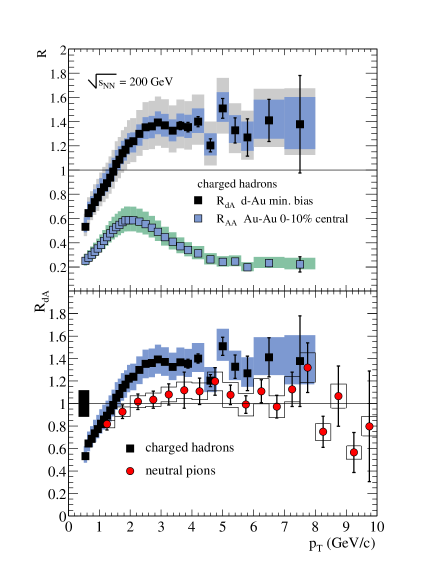
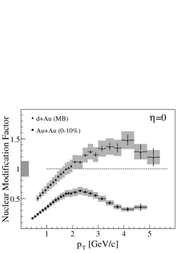
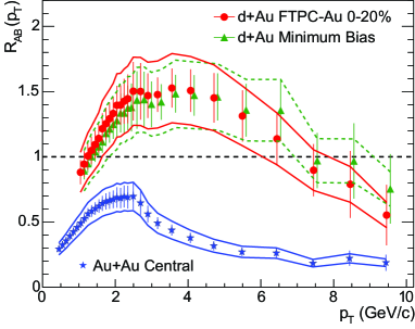
Figure 49: Nuclear modification factor for charged hadrons and neutral pions produced in $d+Au$ and $Au+Au$ collisions at mid-rapidity, as reported by (clockwise from left) PHENIX [51], STAR [53] and BRAHMS [111] collaborations.

The experimental program at RHIC involved $d+Au$ collisions at the center of mass energy $\sqrt{s}=200$ GeV per nucleon. While the above analysis of particle production was, strictly speaking, designed for $pA$ and DIS, we believe that its results can be applied to $d+Au$ collisions as well. $d+Au$ scattering also involves a scattering of a small projectile on a large nucleus, similar to DIS and $pA$. The only assumption we have made in our above analysis was that the saturation scale of the projectile is much smaller than transverse momentum of produced particles, which allowed us to neglect saturation effects in the projectile’s wave function. The fact that deuteron has the atomic number of $A=2$ increases its saturation scale compared to that of a proton by a small factor of $A^{1/3}\approx 1.26$. Therefore, the region of transverse momentum above the deuteron saturation scale, where our analysis is applicable, would still be very wide in $d+Au$ collisions. It is, therefore, a good approximation to apply our above conclusions to $d+Au$ collisions.

Nuclear modification factor for charged hadrons produced in $d+Au$ collisions at mid-rapidity was measured by all four experimental collaborations at RHIC [51, 52, 53, 111]. The data from BRAHMS [111], PHENIX [51] and STAR [53] collaborations is shown in Fig. 49 and the data from PHOBOS collaboration [52] is shown in Fig. 50. One can see that $R^{dAu}$ at mid-rapidity at RHIC exhibits Cronin enhancement [84], in agreement with theoretical expectations of multiple rescattering models, shown in Fig. 36 [85, 32, 86, 87, 88, 89, 64, 62].

Figure 50: Nuclear modification factor for charged hadrons produced in $d+Au$ collisions reported by PHOBOS collaboration [52] in pseudo-rapidity range of $0.2<\eta<1.4$ for four bins of centrality.

The PHOBOS data, presented in Fig. 50 allows one to study $R^{dAu}$ as a function of centrality. Analyzing Eq. (219), along with its asymptotic high-$p_{T}$ limit of Eq. (217), we see that high-$p_{T}$ $R^{dAu}$ in the quasi-classical multiple rescattering approach is an increasing function of $A$, or, equivalently, centrality. These theoretical expectations are confirmed by the data in Fig. 50, where $R^{dAu}$ is clearly an increasing function of the collision centrality.

Figure 51: Predictions of saturation model from [65] (solid and dashed lines) for the total charged particle multiplicity $dN_{ch}/d\eta$ in $d+Au$ collisions compared to the experimental data from [55] as a function of pseudo-rapidity.

An intriguing property of the PHOBOS data from Fig. 50 [52] is that the height of the Cronin maximum in it is much lower than in the data from BRAHMS, PHENIX and STAR collaborations shown in Fig. 49 [111, 51, 53]. The origin of this disagreement appear to be in the fact that PHOBOS was collecting data in the pseudo-rapidity interval of $0.2<\eta<1.4$, whereas the other three collaborations presented the data at $\eta=0$. This decrease of Cronin maximum with increasing rapidity can already be interpreted as a precursor of the suppression predicted by saturation physics shown above in Fig. 41. However, we will postpone this discussion till Sect. 4.2.1 where the data at more forward rapidities will be presented.

Another interesting feature of the $d+Au$ data at mid-rapidity is that other observables, such as integrated charged hadron multiplicity as a function of rapidity [54, 55], appear to be in agreement with saturation/CGC models. In Fig. 51 we show a prediction of saturation model from [65] for the total charged particle multiplicity $dN_{ch}/d\eta$, compared to the data from [55]. The model in [65] uses $k_{T}$-factorization formula for gluon production from Eq. (231) integrated over all $k_{T}$ with the unintegrated gluon distribution on the nucleus “frozen” at a constant at transverse momenta below $Q_{s}$ and falling off as $\sim 1/k_{T}^{2}$ for $k_{T}>Q_{s}$ (for details see [65]). As one can see the agreement between the prediction from [65] and the data is very good.

4.1.2 $dAu$ as a Control Experiment for Quark-Gluon Plasma Production

$dAu$ collisions can be used as a control experiment for formation of quark-gluon plasma (QGP) in $AuAu$ collisions at RHIC. As was originally suggested in [115, 116, 117, 118, 119], creation of a dense hot medium, such as QGP, in high energy heavy ion collisions should lead to a depletion of high-$p_{T}$ particles produced in the collisions. This phenomenon is known as jet quenching [118]. The underlying physics is rather straightforward: high-$p_{T}$ particles produced in the medium would loose energy in interactions with the medium. As a result there would be less high-$p_{T}$ particles produced in the heavy ion collisions than one would naively expect by scaling the number of high-$p_{T}$ particles produced in a $pp$ collisions by the number of elementary nucleon-nucleon collisions $N_{coll}$.

One usually measures this suppression by analyzing the nuclear modification factor for $AA$ collisions, which is defined as

$$R^{AA}\,=\,\frac{\frac{dN^{AA}}{d^{2}k_{T}\,dy}}{N_{coll}\,\frac{dN^{pp}}{d^{2}k_{T}\,dy}}.$$ (324)

Jet quenching due to energy loss of particles in the medium would result in $R^{AA}$ being suppressed. The calculations of such suppression were carried out in [116, 117, 118], where both multiple rescatterings in the medium and medium-induced particle emissions were taken into account.

The data on $R^{AA}$ collected at RHIC was reported in [112, 113, 114, 111]. Here those data are shown in Fig. 49, along with the nuclear modification factor for $d+Au$ collisions. As on can see from Fig. 49, jet quenching was observed in $Au+Au$ collisions at RHIC with $R^{AuAu}<1$ for all measured $p_{T}$.

For jet quenching to become a signal of creation of quark-gluon plasma one has to prove that the observed suppression is really due to energy loss of jets in the produced matter, which would be a final state effect. In principle, jet quenching can be accounted for by the small-$x$ evolution effects in the nuclear wave functions, similar to those described for $pA$ collisions in Sect. 3.2 leading to suppression shown in Fig. 41. Such suppression would be the initial state effect. In fact, it has even been suggested in [61] that the suppression observed in [112, 113, 114, 111] could be due to initial state effects induced by small-$x$ evolution. The initial state suppression should be observable already in $d+Au$ collisions, while the final state energy loss is typical only for $AA$ collisions and should not manifest itself in $d+Au$. In that sense $d+Au$ scattering is a control experiment for QGP formation [120].

The data presented in [51, 52, 53, 111] and shown here in Figs. 49 and 50 clearly indicate absence of suppression in $R^{dAu}$. The Cronin enhancement observed in these data is in agreement with the classical gluon field dynamics for $pA$ collisions of Sect. 3.1: the same initial state classical fields would lead to Cronin-like enhancement of $R^{AA}$ in $AA$ collisions [180]. One can therefore conclude that jet quenching observed for $AA$ collisions in [112, 113, 114, 111] is due to strong final state interactions leading to energy loss of partons in the medium.

Figure 52: Two-particle correlation functions for $pp$, $d+Au$ and central $Au+Au$ collisions measured by STAR collaboration at mid-rapidity [181].

The case for production of hot and dense medium is strengthened by observation of two-particle correlations. In $pp$ collisions a high-$p_{T}$ jet is usually accompanied by another high- or intermediate-$p_{T}$ jet balancing its transverse momentum. This is known as back-to-back jet correlations. In the presence of dense medium absorbing many of the produced jets, such back-to-back correlations should be reduced, and possibly wiped out completely. To see whether this takes place, and to eliminate possible initial state nuclear wave functions effects, one has to study two-particle correlation functions in $Au+Au$, $d+Au$ and $pp$ collisions.

The data on such correlations was reported by the STAR collaboration in [181] and is shown here in Fig. 52. Fig. 52 depicts the correlation function (with constant background subtracted) between a trigger particle (hadron) with $4$ GeV $<p_{T}(trig)<6$ GeV and and associated particle with $2$ GeV $<p_{T}<p_{T}(trig)$ for $pp$, $d+Au$ and central $Au+Au$ collisions as a function of the azimuthal angle $\Delta\phi$ between the two particles. First of all one should note that back-to-back correlations in $Au+Au$ collisions (with $\Delta\phi=\pi$) are completely wiped out in Fig. 52. Secondly, the back-to-back correlations in $pp$ and $d+Au$ are, approximately, the same. Therefore one concludes that disappearance of back-to-back correlations in $Au+Au$ collisions is due to final state effects.

Final state interactions have to be quite strong to eliminate more than half of the jets (see Fig. 49) and completely wipe out their back-to-back correlations (see Fig. 52). Such strong interactions are likely to lead to thermalization of the produced dense medium: if partons interact strongly with high-$p_{T}$ jet particles, they would interact strongly with each other reaching thermal equilibrium. It is therefore quite plausible that $d+Au$ scattering experiments indicate the formation of QGP in $Au+Au$ collisions.

4.2 Forward Rapidity

4.2.1 Suppression at all $p_{T}$: Evidence for the Color Glass Condensate

The results on nuclear modification factor $R^{dAu}$ at forward rapidity were first presented by BRAHMS collaboration in [56]. The final version of the data published in [57] is shown in here in Fig. 53. There the nuclear modification factor $R^{d+Au}$ is plotted as a function of transverse momentum $p_{T}$ for charged hadrons at rapidities $\eta=0,1$ and for negatively charged hadrons at rapidities $\eta=2.2,3.2$. The data of Fig. 53 demonstrates suppression of hadron production as one goes from central towards forward rapidity. We can clearly see that Cronin maximum gradually disappears and suppression sets in as rapidity becomes larger: this clearly confirms the qualitative prediction of Fig. 41 based on Color Glass Condensate/saturation physics [61, 62, 63].

Figure 53: Nuclear modification factor for charged hadrons at rapidities $\eta=0,1$ and for negatively charged hadrons at rapidities $\eta=2.2,3.2$ reported by BRAHMS collaboration in [57].

BRAHMS data on forward suppression in $d+Au$ from [57] is independently confirmed by other RHIC experiments. In Fig. 54 we show the data on hadronic nuclear modification factor $R^{d+Au}$ reported by PHOBOS collaboration in [58]. While PHOBOS collaboration does no have such a wide rapidity acceptance as BRAHMS, one can see the onset of suppression of $R^{d+Au}$ at high $p_{T}$ already at pseudo-rapidities of $\eta=1.0\div 1.4$.

Figure 54: Data on nuclear modification factor $R^{d+Au}$ for hadrons presented by PHOBOS collaboration in [58].

Figure 55: Data on $R^{CP}$ for hadrons presented by PHENIX collaboration in [59].

Figure 56: Data on $R^{d+Au}$ for neutral pions presented by STAR collaboration in [60] superimposed with the BRAHMS collaboration data for negatively charged hadrons from [57].

In Figs. 55 and 56 we show the data presented by PHENIX [59] and STAR [60] collaborations. Instead of $R^{pA}$ from Eq. (208) one sometimes is interested in ratio of particle production rates in central over peripheral collisions, which is defined by

$$R^{CP}(k_{T},y)\,=\,\frac{\frac{1}{N_{coll}}\,\frac{dN^{pA}}{d^{2}k\,dy}\mbox{(central)}}{\frac{1}{N_{coll}}\,\frac{dN^{pA}}{d^{2}k\,dy}\mbox{(peripheral)}}.$$ (325)

As once can see by comparing Eq. (325) to Eq. (208), $R^{CP}$ is very similar to $R^{pA}$, with the difference of using the peripheral $pA$ collisions instead of $pp$ as a reference in the denominator. The conclusions of the above analysis of $R^{pA}$ summarized in Fig. 41 would also apply to $R^{CP}$: we would also expect a transition from Cronin enhancement to suppression in $R^{CP}$ with increasing rapidity.

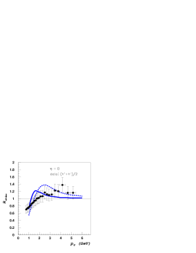
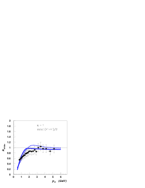
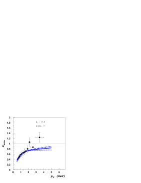
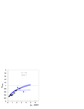
Figure 57: Fit of nuclear modification factor $R_{dAu}$ of charged particles for different rapidities from [122]. In the top two figures, corresponding to $\eta=0,1$, the solid line corresponds to $(h^{-}+h^{+})/2$ contribution calculated with $\kappa=0$ in the isospin-independent approximation, while the dashed line gives the same $(h^{-}+h^{+})/2$ contribution but with $\kappa=1$ GeV. In the lower two plots, corresponding to $\eta=2.2,3.2$, the solid line gives the $h^{-}$ contribution calculated in the constituent quark model with $\kappa=0$, the dashed line gives the same $h^{-}$ contribution for $\kappa=1$ GeV, while the dotted line at $\eta=2.2,3.2$ gives the $(h^{+}+h^{-})/2$ contribution with $\kappa=0$ (see text). Data is from [57].

Fig. 55 plots PHENIX data on $R^{CP}$ for hadrons as a function of $p_{T}$ for three different centrality bins both for forward rapidity ($1.4<\eta<2.2$, denoted by squares) and for backward rapidity ($-2.2<\eta<-1.4$, denoted by circles) [59]. We see that $R^{CP}$ is suppressed at forward pseudo-rapidities $1.4<\eta<2.2$ in agreement with Fig. 53. Fig. 56 presents preliminary STAR data on $R^{d+Au}$ for $\pi^{0}$’s as a function of transverse momentum $p_{T}$ at rapidity $\eta=4$ [60] superimposed with BRAHMS data on negatively charge hadrons at lower rapidities. One can see that suppression gets progressively stronger at forward rapidities, in agreement with Fig. 53, leading to a very strong suppression of $\pi^{0}$’s at $\eta=4$.

Of course the qualitative confirmation of the CGC-based predictions is a very important experimental evidence for saturation/CGC physics. However it is important to demonstrate the quantitative agreement of BRAHMS data [57] with the CGC expectations. A saturation/CGC-based model was constructed in [122], which involved a new parameterization of the dipole-nucleus scattering amplitude $N_{G}$ (see Eq. (328) below and discussion around it), with the saturation scale matching that of the Golec-Biernat–Wüthoff model of DIS on a proton [182]. Together with a simple model for $n_{G}$, the resulting $N_{G}$ from Eq. (328) was used in Eq. (232) to give the gluon production cross section. At forward rapidities high-$p_{T}$ particle production is close to the kinematic limit, which is obtained by demanding that projectile’s Bjorken $x$ is less than $1$, $x_{p}=(k_{T}/\sqrt{s})\,e^{\eta}\leq 1$, leading to $k_{T}\leq\sqrt{s}\,e^{\eta}$. The effective $x_{1}$ is rather large and valence quark contribution becomes important. The latter is given by Eqs. (270) and (271) and was also taken into account in [122]. To compare the quark and gluon production cross sections with the data one indeed needs to convolute them with fragmentation functions. The resulting fit of BRAHMS data from Fig. 53 is shown in Fig. 57 (see also [123]). Since BRAHMS data at rapidities $\eta=0,1$ is for total charged hadrons, while the data at rapidities $\eta=2.2,3.2$ is for negatively charged hadrons, the charge asymmetry issues had to be taken into account [183]. One may also worry that in the given kinematics the saturation-based description of high-$p_{T}$ hadron production in $pp$ collisions may not be well-justified: in that sense the success of the saturation model from [122] in describing particle spectra in $pp$ collisions can be considered as just a parameterization of the $pp$ data. What is important is that saturation correctly describes particle production in $d+Au$ collisions, i.e., the numerator in Eq. (209). To model non-perturbative effects a shift of the saturation scale $\kappa$ was introduced in [122]: however, this shift can be put to zero without significantly impacting the quality of the fit, as one can see from Fig. 57. (The non-perturbative shift appears to improve the agreement with the data at mid-rapidity (the dashed line on the left panel in Fig. 57) indicating that non-perturbative effects may still be important at corresponding values of Bjorken $x$.) We, therefore, conclude that BRAHMS data from Fig. 53 [57] is in both qualitative and quantitative agreement with the saturation/CGC physics.

The model from [122] is based on Eq. (231) with the unintegrated gluon distribution functions calculated in the saturation/CGC approach. In that sense it is consistent with the model of [65] used to describe total charged particle multiplicity in $d+Au$ collisions, as shown in Fig. 51. Both models are inspired by saturation physics, but reflect different aspects of it: the model from [122] deals with the high-$p_{T}$ hadronic spectra, and is, therefore, more accurate at high-$p_{T}$. At the same time the model in [65] concentrates on total particle multiplicity, which is most sensitive to low-$p_{T}$ hadron production: therefore, that model is more precise at low-$p_{T}$.

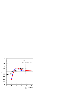
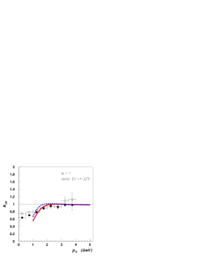
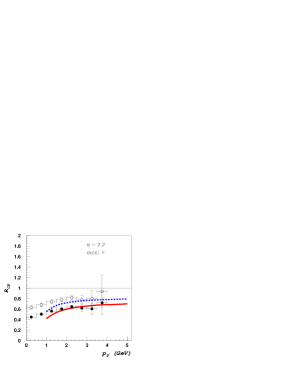
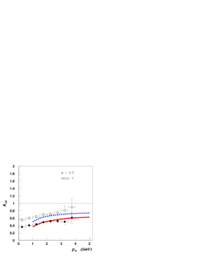
Figure 58: Data from [57] on nuclear modification factor $R_{CP}$ of charged particles $(h^{+}+h^{-})/2$ for rapidities $\eta=0,1$ and of negatively charged particles $h^{-}$ for $\eta=2.2,3.2$ superimposed with the results of the model from [122]. Full and open dots, described by the solid and dashed lines correspondingly, give the ratio of particle yields in 0-20$\%$ and 30-50$\%$ centrality events correspondingly divided by the yields from 60-80$\%$ centrality events scaled by the mean number of binary collisions [57].

In Fig. 58 we show BRAHMS data on $R^{CP}$ for the same rapidities as in Fig. 57. Full dots correspond to more central collisions, while open dots correspond to more peripheral collisions (see the caption of Fig. 58). One can see that, in agreement with the expectation of saturation/CGC (see Sect. 3.1), the Cronin maximum at $\eta=0$ is an increasing function of centrality. At forward rapidities the centrality dependence changes: $R^{CP}$ becomes a decreasing function of centrality, again in agreement with expectations of saturation/CGC approach (see Sect. 3.2). On top of this qualitative agreement between the data and the theory of CGC, in Fig. 58 we observe quantitative correspondence of the data and the results of the saturation-inspired model from [122].

There have been several attempts to explain the suppression of particle production from Fig. 53 in the frameworks alternative or parallel to CGC. In [183, 184] the suppression of [57] was analyzed in the framework of standard shadowing models. The conclusion of [183] was that the observed suppression is much stronger than one would anticipate using the common parameterizations of nuclear shadowing. In [185] it was argued that multiple rescattering in the nuclei would lead to observed suppression: however, this conclusion appears to be in contradiction with our Sect. 3.1, where we prove that multiple rescatterings lead to enhancement of the nuclear modification factor. Recently a new model was proposed in [186] in which the origin of suppression in Fig. 53 was attributed to energy conservation which was imposed by Sudakov from-factors. The model of [186] includes both multiple rescatterings and small-$x$ evolution: hence at the moment the conceptual differences between the CGC approach and the model from [186] are not clear. Parton recombination models also appear to be able to accommodate the data by completely redefining the hadronization mechanism [187].

4.2.2 Future Experimental Tests

Despite the successes of the Color Glass Condensate in predicting the suppression of the hadron production cross section in proton (deuteron)-nucleus collisions as compared to proton-proton collisions in the forward rapidity region at RHIC and the change of centrality dependence as one goes from mid to forward rapidity, one would like to quantitatively understand to which degree CGC is the dominant physics at forward rapidity RHIC and LHC collisions and possibly at mid-rapidity LHC collisions. So far, the main evidence for CGC at RHIC comes from the $p_{T}$ spectrum of single inclusive hadron production in deuteron-gold collisions in the forward rapidity region.

A difficulty with a quantitative understanding of the physics behind the observed suppression of the hadron spectra in deuteron-nucleus collisions at RHIC is that hadronization by its nature is non-perturbative and is not well-understood from first principles. To avoid non-perturbative physics or to, at least, minimize its effects, one needs to consider high $p_{T}$ processes. Exactly at what $p_{T}$ non-perturbative physics can be safely neglected can not be addressed by pQCD and one needs experimental input. The RHIC data on transverse momentum spectra of pions produced in proton-proton collisions in forward rapidity suggest that NLO pQCD works well down to $p_{T}\sim 1.5-2$ GeV [188]. Therefore one may expect the weak coupling methods employed by CGC to work at similar $p_{T}$’s for differential cross sections, even though perturbative approaches usually work much better for ratios of cross sections due to possible (partial) cancellations of large corrections in both the numerator and the denominator.

The experimental situation is complicated by the fact the forward rapidity data published by BRAHMS is for negatively charged hadrons, production of which is suppressed, as compared to neutral or charge averaged hadrons, in proton-proton collisions. This can bias the nuclear modification factor as pointed out in [183]. However, the preliminary data on neutral pion production from STAR at rapidity $\eta=4$ shown above in Fig. 56 demonstrates clear suppression up to $p_{T}\approx 2$ GeV. If this preliminary STAR data is confirmed, it will help clarify the role of isospin effects in the observed suppression of the hadron spectra at forward rapidity.

The situation will improve drastically at LHC where due to an order of magnitude higher center of mass energy, the saturation scale is expected to be higher so that the weak coupling methods of CGC will be much more reliable and the available phase space in transverse momenta will be much larger even at rapidities as high as $5-6$ which should eliminate or minimize phase space edge effects even for moderately large transverse momenta.

Nevertheless, one can further test applicability of the Color Glass Condensate at RHIC by considering its electromagnetic signatures, for example in photon and dilepton production considered earlier. As noted above, the CGC building blocks for single particle production cross sections in proton-nucleus collisions are the fundamental and adjoint dipole cross sections, describing the scattering of quarks and gluons from the target. Therefore, one can ”measure” or (more precisely) constrain the dipole cross section in one process and then use it to make predictions for other processes. This is in direct analogy with particle production cross sections in pQCD where one has universal (process independent) ingredients in the form of distribution and fragmentation functions, which are measured in one process and then used to make predictions for other processes, which give rise to the predictive power of the theory.

Here we consider models of the dipole cross section (we consider those which include the small $x$ evolution governed by JIMWLK or BK equations only) which have been used to fit the data, either in DIS at HERA or pA at RHIC. We then use these models to make predictions for photon and dilepton production cross sections and their modification factors at RHIC and LHC. We show that measuring the photon production cross section at RHIC can impose significant constraints on the models of the dipole cross section and further clarify the role of the Color Glass Condensate at RHIC.

The first model of the dipole cross section we consider is that of Iancu, Itakura and Munier [189] which was used to fit the proton structure functions at HERA. It has the correct behavior in the saturation region and in the geometric scaling region but does not have the correct double logarithmic limit built in. Furthermore, it is fit to the data on proton targets and not on nuclear targets. The IIM model of the dipole cross section is

$$\int d^{2}b\,N(r_{T},b_{T},\ln 1/x_{g})\,\equiv\,\pi\,R^{2}\,\,{\cal N}\,(x_{g},r_{T}Q_{s})$$ (326)

where

$${\cal N}\,(x_{g},r_{T}Q_{s})=1-e^{-a\ln^{2}(b\,r_{T}Q_{s})},\,\,\,\,\,\,\,\,\,\,\mbox{for}\hskip 14.22636ptr_{T}\,Q_{s}>2$$

and

$${\cal N}\,(x_{g},r_{T}Q_{s})={\cal N}_{0}\exp\Bigg{\{}2\ln({r_{T}Q_{s}\over 2})\bigg{[}\gamma_{s}+{\ln 2/r_{T}Q_{s}\over\kappa\lambda\ln 1/x_{g}}\bigg{]}\Bigg{\}},\,\,\,\,\,\,\,\,\,\,\mbox{for}\hskip 14.22636ptr_{T}\,Q_{s}\leq 2$$ (327)

The constants $a,b$ are determined by matching the solutions at $r_{T}\,Q_{s}=2$ while $\gamma_{s}=0.63$ and $\kappa=9.9$ are determined from LO BFKL. The form of the saturation scale $Q_{s}^{2}$ is taken to be $Q_{s}^{2}\equiv(x_{0}/x)^{\lambda}$ GeV² with $x_{0},\lambda,R,{\cal N}_{0}$ determined from fitting the HERA data on proton structure function $F_{2}$ [189].

Figure 59: Invariant mass dependence of the nuclear modification factor for dilepton production in proton(deuteron)-nucleus scattering at RHIC.

This model of the dipole cross section was used in [121] to make predictions for the transverse momentum integrated nuclear modification factor $R_{pA}$ for dilepton production cross section in deuteron (proton)–nucleus collisions at RHIC. (For the $p_{T}$-dependence of dilepton $R_{pA}$ see [100].) Here we show the main result of [121] for the nuclear modification factor for central collisions and at $y=2.2$ in Fig. 59 which shows a clear suppression in analogy with the nuclear modification factor in hadron production at RHIC that can be understood as being due to the quantum evolution of the dipole-nucleus cross section, present in both hadron and dilepton production cross sections. In the case of a deuteron projectile, nuclear shadowing (anti-shadowing) of the deuteron wave function is included by using the HKM parameterization [190].

We also show the nuclear modification factor for central collisions and at rapidity $y=5$ for the integrated over transverse momentum dilepton nuclear modification factor at LHC as a function of the dilepton invariant mass $M$ in Fig. 60, where again a similar suppression is seen. Here one can extend the calculations to much higher dilepton masses since the saturation scale is very large due to the large forward rapidity and the order of magnitude increase in the center of mass energy at LHC as compared to RHIC.

Figure 60: Invariant mass dependence of the nuclear modification factor for dilepton production in proton-nucleus scattering at LHC.

We note that the IIM parameterization of the dipole cross section is originally done for a proton target. Here we have assumed a simple scaling of the dipole profile function by $A^{1/3}$ in order to use it for nuclear targets. There is another parameterization of the dipole cross section, due to Kharzeev, Tuchin and one of the authors [122], which has been used to fit the hadron production data in deuteron-nucleus collisions at RHIC. This model has the advantage that it has the correct high $p_{t}$ limit built in, unlike the IIM parameterization. It is given by

$$N(r_{T},x_{g})\,=\,1-\exp\left[-\frac{1}{4}\left(r_{T}^{2}\frac{C_{F}}{N_{c}}\,Q_{s}^{2}\right)^{\gamma(x_{g},r_{T}^{2})}\right].$$ (328)

where the anomalous dimension $\gamma(y,r_{T}^{2})$ is parameterized as

$$\gamma(y,r_{T}^{2})\,=\,\frac{1}{2}\left(1+\frac{\xi(y,r_{T}^{2})}{\xi(y,r_{T}^{2})+\sqrt{2\,\xi(y,r_{T}^{2})}+7\zeta(3)\,c}\right),$$ (329)

with $y=\ln 1/x_{g}$ and

$$\xi(y,r_{T}^{2})\,=\,\frac{\ln\left[1/(r_{T}^{2}\,Q_{s0}^{2})\right]}{(\lambda/2)(y-y_{0})}\,,$$ (330)

and $c$ is a constant fitted to the data. This parameterization has the correct high-$p_{T}$ behavior where $\gamma\rightarrow 1$. In Fig. 61 we show the profile function for the two dipole parameterizations as a function of the dimensionless variable $r_{T}Q_{s}$ for a nuclear target for $x_{g}=1.6\,\times\,10^{-4}$ (which corresponds to $p_{T}=1.5$ GeV at $y=3.8$ at RHIC). Clearly, the two dipole profiles are quite different.

Figure 61: Quark anti-quark dipole profile for a nuclear target.

We now use the two parameterizations of the dipole cross section to calculate the photon production cross section in deuteron-gold collisions at RHIC. To get the cross section, we need to convolute the partonic production cross section in (280) with the quark (and anti-quark) distribution function in a deuteron. We therefore use [96]

$${d\sigma^{d(A)\,A\rightarrow\gamma(k_{T},y_{\gamma})\,X}\over d^{2}b\,d^{2}k\,dy_{\gamma}}\!\!\! = \!\!\!{1\over(2\pi)^{2}}\sum_{f}\int dx_{q}\,[q_{f}(x_{q},k_{T}^{2})+\bar{q}_{f}(x_{q},k_{T}^{2})]\,{D_{\gamma/q}(z,k_{T}^{2})\over z}\sigma_{dipole}^{F}(x_{g},{k_{T}\over z},{\underline{b}})$$ (331)

to calculate the nuclear modification factor for photon production in deuteron-gold collisions at RHIC at $y=3.8$ and for the most central collisions. This will be eventually measured at RHIC by the STAR detector.

It is clear that the two parameterizations lead to quite different results shown in Fig. 62. This may be understood to be due to the different dipole shapes in the two approaches, so that a future measurement of this ratio can help constrain the models of the dipole cross section. Each parameterization of the dipole cross section has its advantages and disadvantages. For example, the IIM parameterization is a fit to the proton structure function, which involves a convolution of the dipole cross section with the photon wave function squared. Therefore, the dipole cross section is weighed preferentially in the physical cross section and some dipole sizes play a bigger role than others. The KKT parameterization on the other hand is a fit to particle production data which is a less inclusive observable than a fully inclusive structure function and therefore is more constraining on the dipole cross section. However, it is partly complicated by hadronization and the need for a convolution with the hadron fragmentation functions. Electromagnetic signatures of the Color Glass Condensate therefore offer a more precise means by which the quantitative aspects of CGC may be probed.

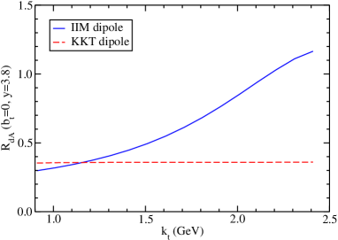
Figure 62: Nuclear modification factor for photon production.

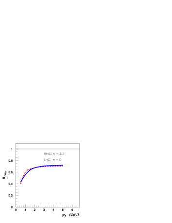
Figure 63: Nuclear modification factor $R^{pA}$ of charged particles $(h^{+}+h^{-})/2$ at LHC energies $\sqrt{s}=5500$ GeV at mid-rapidity $\eta=0$ as predicted in [122] (dashed line) versus $R^{dAu}$ of $(h^{+}+h^{-})/2$ for RHIC energies $\sqrt{s}=200$ GeV at $\eta=3.2$ (solid line).

Having a parameterization of the dipole-nucleus scattering amplitude $N$ should allow one to make predictions for particle production at LHC. In Fig. 63 we present a prediction from [122] for the nuclear modification factor $R^{pA}$ of charged particles at mid-rapidity at LHC (dashed line). It appears that the amount of suppression to be seen at mid-rapidity $pA$ collisions at LHC is roughly equal to the currently observed at forward rapidity $d+A$ collisions at RHIC (solid line in Fig. 63). It would be very interesting to verify this prediction. If suppression at mid-rapidity $pA$ collisions at LHC is observed, then one would be able to appreciate how special RHIC energy range is: while the center of mass collisions energy at RHIC is high, it is still low enough to have Cronin enhancement at mid-rapidity in $d+Au$ collisions, allowing to use $d+Au$ as a control experiment for the suppression of particle production observed in $Au+Au$ indicating creation of quark-gluon plasma.

Figure 64: Two-gluon production in $pA$ collision in $k_{T}$-factorization approximation, which includes linear BFKL evolution only.

Another interesting experimental test of Color Glass Condensate physics is in measuring two-particle correlations. While the exact numerical analysis of Eq. (291) leading to numerical predictions to be verified experimentally has not been done yet, one can use the fact that for $k_{1T},k_{2T}\gg Q_{s}$ all the higher-twist multiple rescattering effects are not important and the two-gluon production cross section (291) (generalized to $pA$) reduces to the following expression for gluon multiplicity [176]

$$\frac{dN^{p\,A}}{d^{2}k_{1}\,dy_{1}\,d^{2}k_{2}\,dy_{2}\,d^{2}B}({\underline{x}}_{0{\tilde{0}}})\bigg{|}_{y_{2}\gg y_{1}}\,=\,\frac{\alpha_{s}^{2}\,N_{c}}{\pi^{2}\,C_{F}}\,\frac{1}{{\underline{k}}_{1}^{2}\,{\underline{k}}_{2}^{2}}\,\int d^{2}q_{1}\,d^{2}q_{2}\,\phi_{p}({\underline{q}}_{2}^{2},Y-y)\,f({\underline{k}}_{2}-{\underline{q}}_{2},{\underline{q}}_{1},y_{2}-y_{1})$$

$$\times\,\phi_{A}(({\underline{k}}_{1}-{\underline{q}}_{1})^{2},y_{1}),$$ (332)

where $f({\underline{k}}_{2}-{\underline{q}}_{2},{\underline{q}}_{1},y_{2}-y_{1})$ is given by the BFKL equation (21) with the initial conditions from Eq. (20) and both $\phi_{p}$ and $\phi_{A}$ have linear evolution only. Eq. (332) is the expression for two-gluon production in $k_{T}$-factorization formalism [176] applied to $pA$ collisions. It is illustrated in Fig. 64.

Following Kharzeev, Levin, and McLerran [101], we apply Eq. (332) to the case when the rapidity interval between the two produced gluons is very large. For instance, in RHIC $d+Au$ kinematics, we are interested in the case when one of the gluons is produced at mid-rapidity and the other one is produced at forward deuteron rapidity. This is the case of Mueller-Navelet jets, which were originally proposed in [177] by Mueller and Navelet as an observable allowing to study experimentally the BFKL dynamics.

Figure 65: Prediction from [101] of suppression of back-to-back correlations of high-$p_{T}$ hadrons produced in $d+Au$ collisions as compared to $pp$ collisions.

Since Eq. (332) also applies to gluon production in $pp$ collisions, one can compare the strength of back-to-back correlations in $pA$ and $pp$ collisions with one gluon at mid-rapidity and the other one at forward rapidity. The authors of [101] argued that BFKL evolution between the two produced gluons would deplete back-to-back correlations of produced gluons due to onset of anomalous dimension (163) in $pA$ scattering. The effect is similar to suppression in $R^{pA}$ discussed above in Sect. 3.2. The resulting prediction for suppression of back-to-back correlations from [101] is shown in Fig. 65, where the two-particle correlator is plotted as a function of the azimuthal angle between the particles for $d+Au$ and $pp$ collisions (with a constant background subtracted). Once can see that the strength of back-to-back correlations should be reduced due to the anomalous dimension effects in $d+Au$ collisions. Experimental verification of the qualitative behavior predicted in Fig. 65 by the authors of [101] would be an interesting and important test of CGC. Preliminary results from STAR collaboration [178] appear to confirm the qualitative expectation of suppression of back-to-back correlations for particles produced with a large rapidity interval between them, but more experimental tests are needed to reach a conclusion.

5 Conclusions

In writing a review of a rapidly developing field, one is bound to omit recent developments, which happen in parallel to the writing of the article. The topic of pomeron loop corrections to JIMWLK and BK evolution equations has received a lot of attention in the recent literature [124, 125, 126, 127, 128]. Pomeron loops are corrections to the non-linear evolution equations which are not enhanced by powers of color charge density, or, equivalently, powers of $A$. A typical pomeron loop brings in an extra (parametric) factor of $\alpha_{s}^{2}\,\exp\{(\alpha_{P}-1)\,Y\}$ [21, 24]. Such corrections become important when $\alpha_{s}^{2}\,\exp\{(\alpha_{P}-1)\,Y\}\,\sim\,1$. Therefore, JIMWLK and BK evolution equations are valid up to rapidities [21, 24]

$$Y\,\leq\,Y_{loop}\,=\,\frac{1}{\alpha_{P}-1}\,\ln\frac{1}{\alpha_{s}^{2}}.$$ (333)

Eq. (333), along with Eq. (3), describes the applicability region of JIMWLK and BK evolution equations. For rapidities higher than $Y_{loop}$ pomeron loop corrections become important and have to be included. In the recent papers [124, 125, 126, 127, 128] corrections to JIMWLK evolution were discussed, which would take into account pomeron loop contributions. The consequences of pomeron loop corrections for observables in $pA$ collisions are not clear at present.

Another important class of processes which we have omitted here are the exclusive and semi-exclusive processes. In the quasi-classical approximation the diffractive DIS structure functions were calculated in [129, 130]. In the framework of dipole model one can construct an evolution equation governing single diffractive dissociation amplitudes for DIS, as it was done in [131]. The results of both [129, 130] and [131] can easily be generalized to $pA$ collisions. Diffractive particle production was calculated for both DIS and $pA$ in the quasi-classical approximation in [132]. Unfortunately, due to limited detector capabilities, it appears to be very difficult, if not impossible, to measure these exclusive processes at RHIC. Since our review here is dedicated to RHIC physics we had to omit such processes.

We conclude by pointing out once again that we have reviewed the state of the field at the moment of writing. Future developments are likely to bring in many new exciting results, possibly modifying some of the discussed conclusions and adding on to the material presented here.

References

- [1] L. V. Gribov, E. M. Levin and M. G. Ryskin, Phys. Rept. 100, 1 (1983).
- [2] A. H. Mueller and J. w. Qiu, Nucl. Phys. B 268, 427 (1986).
- [3] L. D. McLerran and R. Venugopalan, Phys. Rev. D 49, 2233 (1994) [arXiv:hep-ph/9309289]; Phys. Rev. D 49, 3352 (1994) [arXiv:hep-ph/9311205]; Phys. Rev. D 50, 2225 (1994) [arXiv:hep-ph/9402335].
- [4] Y. V. Kovchegov, Phys. Rev. D 54, 5463 (1996) [arXiv:hep-ph/9605446].
- [5] Y. V. Kovchegov, Phys. Rev. D 55, 5445 (1997) [arXiv:hep-ph/9701229].
- [6] J. Jalilian-Marian, A. Kovner, L. D. McLerran and H. Weigert, Phys. Rev. D 55, 5414 (1997) [arXiv:hep-ph/9606337].
- [7] J. Jalilian-Marian, A. Kovner, A. Leonidov and H. Weigert, Nucl. Phys. B 504, 415 (1997) [arXiv:hep-ph/9701284].
- [8] J. Jalilian-Marian, A. Kovner, A. Leonidov and H. Weigert, Phys. Rev. D 59, 014014 (1999) [arXiv:hep-ph/9706377].
- [9] J. Jalilian-Marian, A. Kovner and H. Weigert, Phys. Rev. D 59, 014015 (1999) [arXiv:hep-ph/9709432].
- [10] J. Jalilian-Marian, A. Kovner, A. Leonidov and H. Weigert, Phys. Rev. D 59, 034007 (1999) [Erratum-ibid. D 59, 099903 (1999)] [arXiv:hep-ph/9807462].
- [11] A. Kovner and J. G. Milhano, Phys. Rev. D 61, 014012 (2000) [arXiv:hep-ph/9904420].
- [12] A. Kovner, J. G. Milhano and H. Weigert, Phys. Rev. D 62, 114005 (2000) [arXiv:hep-ph/0004014].
- [13] E. Iancu, A. Leonidov and L. D. McLerran, Nucl. Phys. A 692, 583 (2001) [arXiv:hep-ph/0011241].
- [14] E. Iancu, A. Leonidov and L. D. McLerran, Phys. Lett. B 510, 133 (2001) [arXiv:hep-ph/0102009].
- [15] E. Iancu and L. D. McLerran, Phys. Lett. B 510, 145 (2001) [arXiv:hep-ph/0103032].
- [16] E. Ferreiro, E. Iancu, A. Leonidov and L. McLerran, Nucl. Phys. A 703, 489 (2002) [arXiv:hep-ph/0109115].
- [17] H. Weigert, Nucl. Phys. A 703, 823 (2002) [arXiv:hep-ph/0004044].
- [18] K. Rummukainen and H. Weigert, Nucl. Phys. A 739, 183 (2004) [arXiv:hep-ph/0309306].
- [19] A. H. Mueller, Nucl. Phys. B 415, 373 (1994).
- [20] A. H. Mueller and B. Patel, Nucl. Phys. B 425, 471 (1994) [arXiv:hep-ph/9403256].
- [21] A. H. Mueller, Nucl. Phys. B 437, 107 (1995) [arXiv:hep-ph/9408245].
- [22] Z. Chen and A. H. Mueller, Nucl. Phys. B 451, 579 (1995).
- [23] I. Balitsky, Nucl. Phys. B 463, 99 (1996) [arXiv:hep-ph/9509348]; arXiv:hep-ph/9706411; Phys. Rev. D 60, 014020 (1999) [arXiv:hep-ph/9812311].
- [24] Y. V. Kovchegov, Phys. Rev. D 60, 034008 (1999) [arXiv:hep-ph/9901281]; Phys. Rev. D 61, 074018 (2000) [arXiv:hep-ph/9905214].
- [25] M. Froissart, Phys. Rev. 123, 1053 (1961).
- [26] J. Bartels, J. Phys. G 19, 1611 (1993); J. Bartels, H. Lotter and M. Vogt, Phys. Lett. B 373, 215 (1996) [arXiv:hep-ph/9511399].
- [27] E. A. Kuraev, L. N. Lipatov and V. S. Fadin, Sov. Phys. JETP 45, 199 (1977) [Zh. Eksp. Teor. Fiz. 72, 377 (1977)]; I. I. Balitsky and L. N. Lipatov, Sov. J. Nucl. Phys. 28, 822 (1978) [Yad. Fiz. 28, 1597 (1978)].
- [28] A. Kovner, L. D. McLerran and H. Weigert, Phys. Rev. D 52, 3809 (1995) [arXiv:hep-ph/9505320].
- [29] A. Kovner, L. D. McLerran and H. Weigert, Phys. Rev. D 52, 6231 (1995) [arXiv:hep-ph/9502289].
- [30] Yu. V. Kovchegov and D. H. Rischke, Phys. Rev. C 56, 1084 (1997) [arXiv:hep-ph/9704201].
- [31] M. Gyulassy and L. D. McLerran, Phys. Rev. C 56, 2219 (1997) [arXiv:nucl-th/9704034].
- [32] Y. V. Kovchegov and A. H. Mueller, Nucl. Phys. B 529, 451 (1998) [arXiv:hep-ph/9802440].
- [33] A. Dumitru and L. D. McLerran, Nucl. Phys. A 700, 492 (2002) [arXiv:hep-ph/0105268].
- [34] Yu. V. Kovchegov and K. Tuchin, Phys. Rev. D 65, 074026 (2002) [arXiv:hep-ph/0111362].
- [35] F. Gelis and J. Jalilian-Marian, Phys. Rev. D 67, 074019 (2003) [arXiv:hep-ph/0211363]; A. Dumitru and J. Jalilian-Marian, Phys. Lett. B 547, 15 (2002) [arXiv:hep-ph/0111357]; Phys. Rev. Lett. 89, 022301 (2002) [arXiv:hep-ph/0204028].
- [36] J. P. Blaizot, F. Gelis and R. Venugopalan, Nucl. Phys. A 743, 57 (2004) [arXiv:hep-ph/0402257]; Nucl. Phys. A 743, 13 (2004) [arXiv:hep-ph/0402256]; F. Gelis and R. Venugopalan, Phys. Rev. D 69, 014019 (2004) [arXiv:hep-ph/0310090].
- [37] A. Dumitru and J. Jalilian-Marian, Phys. Rev. Lett. 89, 022301 (2002) [arXiv:hep-ph/0204028].
- [38] F. Gelis and A. Peshier, Nucl. Phys. A 697, 879 (2002) [arXiv:hep-ph/0107142].
- [39] A. Dumitru and J. Jalilian-Marian, Phys. Lett. B 547, 15 (2002) [arXiv:hep-ph/0111357].
- [40] F. Gelis and J. Jalilian-Marian, Phys. Rev. D 67, 074019 (2003) [arXiv:hep-ph/0211363].
- [41] Y. V. Kovchegov, Nucl. Phys. A 692, 557 (2001) [arXiv:hep-ph/0011252].
- [42] I. Balitsky, Phys. Rev. D 70, 114030 (2004) [arXiv:hep-ph/0409314].
- [43] A. Krasnitz and R. Venugopalan, Phys. Rev. Lett. 84, 4309 (2000) [arXiv:hep-ph/9909203]; Phys. Rev. Lett. 86, 1717 (2001) [arXiv:hep-ph/0007108]; A. Krasnitz, Y. Nara and R. Venugopalan, Phys. Rev. Lett. 87, 192302 (2001) [arXiv:hep-ph/0108092]; Nucl. Phys. A 727, 427 (2003) [arXiv:hep-ph/0305112]; Nucl. Phys. A 717, 268 (2003) [arXiv:hep-ph/0209269].
- [44] T. Lappi, Phys. Rev. C 67, 054903 (2003) [arXiv:hep-ph/0303076].
- [45] J. F. Gunion and G. Bertsch, Phys. Rev. D 25, 746 (1982).
- [46] L. N. Lipatov, Nucl. Phys. B 365, 614 (1991).
- [47] A. H. Mueller, arXiv:hep-ph/0307265.
- [48] E. Iancu, A. Leonidov and L. McLerran, arXiv:hep-ph/0202270.
- [49] E. Iancu and R. Venugopalan, arXiv:hep-ph/0303204.
- [50] H. Weigert, arXiv:hep-ph/0501087.
- [51] S. S. Adler et al. [PHENIX Collaboration], Phys. Rev. Lett. 91, 072303 (2003) [arXiv:nucl-ex/0306021].
- [52] B. B. Back et al. [PHOBOS Collaboration], Phys. Rev. Lett. 91, 072302 (2003) [arXiv:nucl-ex/0306025].
- [53] J. Adams et al. [STAR Collaboration], Phys. Rev. Lett. 91, 072304 (2003) [arXiv:nucl-ex/0306024].
- [54] B. B. Back et al. [PHOBOS Collaboration], Phys. Rev. Lett. 93, 082301 (2004) [arXiv:nucl-ex/0311009].
- [55] I. Arsene et al. [BRAHMS Collaboration], Phys. Rev. Lett. 94, 032301 (2005) [arXiv:nucl-ex/0401025].
- [56] R. Debbe, [BRAHMS Collaboration], talk given at the APS DNP Meeting at Tucson, AZ, October, 2003; R. Debbe [BRAHMS Collaboration], arXiv:nucl-ex/0403052.
- [57] I. Arsene et al. [BRAHMS Collaboration], Phys. Rev. Lett. 93, 242303 (2004) [arXiv:nucl-ex/0403005].
- [58] B. B. Back et al. [PHOBOS Collaboration], Phys. Rev. C 70, 061901 (2004) [arXiv:nucl-ex/0406017].
- [59] S. S. Adler et al. [PHENIX Collaboration], Phys. Rev. Lett. 94, 082302 (2005) [arXiv:nucl-ex/0411054].
- [60] G. Rakness [STAR Collaboration], talks given at XXXXth Rencontres de Moriond, “QCD and Hadronic Interactions at High Energy”, March 12-19, 2005, La Thuile, Italy and at the XIII International Workshop on Deep Inelastic Scattering (DIS2005), April 27 - May 1, 2005, Madison, Wisconsin, USA; see also L. S. Barnby [STAR Collaboration], [arXiv:nucl-ex/0404027].
- [61] D. Kharzeev, E. Levin and L. McLerran, Phys. Lett. B 561, 93 (2003) [arXiv:hep-ph/0210332].
- [62] D. Kharzeev, Y. V. Kovchegov and K. Tuchin, Phys. Rev. D 68, 094013 (2003) [arXiv:hep-ph/0307037].
- [63] J. L. Albacete, N. Armesto, A. Kovner, C. A. Salgado and U. A. Wiedemann, Phys. Rev. Lett. 92, 082001 (2004) [arXiv:hep-ph/0307179].
- [64] R. Baier, A. Kovner and U. A. Wiedemann, Phys. Rev. D 68, 054009 (2003) [arXiv:hep-ph/0305265].
- [65] D. Kharzeev, E. Levin and M. Nardi, Nucl. Phys. A 730, 448 (2004) [Erratum-ibid. A 743, 329 (2004)] [arXiv:hep-ph/0212316].
- [66] E. Levin, arXiv:hep-ph/9710546.
- [67] A. H. Mueller, Nucl. Phys. B 335, 115 (1990).
- [68] R. J. Glauber, Phys. Rev. 100, 242 (1955).
- [69] C. S. Lam and G. Mahlon, Phys. Rev. D 61, 014005 (2000) [arXiv:hep-ph/9907281]; Phys. Rev. D 62, 114023 (2000) [arXiv:hep-ph/0007133]; Phys. Rev. D 64, 016004 (2001) [arXiv:hep-ph/0102337].
- [70] B. L. Ioffe, JETP Lett. 9, 163 (1969); 10, 143 (1969); Phys. Lett. 30B, 123 (1969); Y. V. Kovchegov and M. Strikman, Phys. Lett. B 516, 314 (2001) [arXiv:hep-ph/0107015] and references therein.
- [71] A. M. Stasto, K. Golec-Biernat and J. Kwiecinski, Phys. Rev. Lett. 86, 596 (2001) [arXiv:hep-ph/0007192].
- [72] E. Levin and K. Tuchin, Nucl. Phys. B 573, 833 (2000) [arXiv:hep-ph/9908317].
- [73] E. Iancu, K. Itakura and L. McLerran, Nucl. Phys. A 708, 327 (2002) [arXiv:hep-ph/0203137].
- [74] A. H. Mueller and D. N. Triantafyllopoulos, Nucl. Phys. B 640, 331 (2002) [arXiv:hep-ph/0205167]; D. N. Triantafyllopoulos, Nucl. Phys. B 648, 293 (2003) [arXiv:hep-ph/0209121].
- [75] A. H. Mueller, arXiv:hep-ph/0301109.
- [76] S. Munier and R. Peschanski, Phys. Rev. Lett. 91, 232001 (2003) [arXiv:hep-ph/0309177]; Phys. Rev. D 70, 077503 (2004) [arXiv:hep-ph/0401215]; C. Marquet, R. Peschanski and G. Soyez, arXiv:hep-ph/0502020.
- [77] M. Braun, Eur. Phys. J. C 16, 337 (2000) [arXiv:hep-ph/0001268].
- [78] K. Golec-Biernat, L. Motyka and A. M. Stasto, Phys. Rev. D 65, 074037 (2002) [arXiv:hep-ph/0110325]; K. Golec-Biernat and A. M. Stasto, Nucl. Phys. B 668, 345 (2003) [arXiv:hep-ph/0306279].
- [79] E. Gotsman, E. Levin, M. Lublinsky and U. Maor, Eur. Phys. J. C 27, 411 (2003) [arXiv:hep-ph/0209074]; E. Levin and M. Lublinsky, Phys. Lett. B 521, 233 (2001) [arXiv:hep-ph/0108265]; E. Levin and M. Lublinsky, Nucl. Phys. A 696, 833 (2001) [arXiv:hep-ph/0104108]; M. Lublinsky, E. Gotsman, E. Levin and U. Maor, Nucl. Phys. A 696, 851 (2001) [arXiv:hep-ph/0102321].
- [80] M. Lublinsky, Eur. Phys. J. C 21, 513 (2001) [arXiv:hep-ph/0106112].
- [81] J. L. Albacete, N. Armesto, J. G. Milhano, C. A. Salgado and U. A. Wiedemann, arXiv:hep-ph/0502167; Phys. Rev. D 71, 014003 (2005) [arXiv:hep-ph/0408216].
- [82] B. Z. Kopeliovich, A. V. Tarasov and A. Schafer, Phys. Rev. C 59, 1609 (1999) [arXiv:hep-ph/9808378].
- [83] A. Kovner and U. A. Wiedemann, Phys. Rev. D 64, 114002 (2001) [arXiv:hep-ph/0106240].
- [84] J. W. Cronin, H. J. Frisch, M. J. Shochet, J. P. Boymond, R. Mermod, P. A. Piroue and R. L. Sumner, Phys. Rev. D 11, 3105 (1975).
- [85] B. Z. Kopeliovich, J. Nemchik, A. Schafer and A. V. Tarasov, Phys. Rev. Lett. 88, 232303 (2002) [arXiv:hep-ph/0201010].
- [86] X. N. Wang, Phys. Rev. Lett. 81 (1998) 2655; M. Gyulassy and P. Levai, Phys. Lett. B 442 (1998) 1; X. N. Wang, Phys. Rev. C 61 (2000) 064910.
- [87] E. Wang and X. N. Wang, Phys. Rev. C 64 (2001) 034901; Y. Zhang, G. Fai, G. Papp, G. G. Barnafoldi and P. Levai, Phys. Rev. C 65 (2002) 034903; I. Vitev and M. Gyulassy, Phys. Rev. Lett. 89 (2002) 252301.
- [88] I. Vitev, Phys. Lett. B 562, 36 (2003); [arXiv:nucl-th/0302002].
- [89] X. N. Wang, Phys. Lett. B 565 (2003) 116; X. N. Wang, arXiv:nucl-th/0305010; X. Zhang and G. Fai, arXiv:hep-ph/0306227. G. G. Barnafoldi, G. Papp, P. Levai and G. Fai, arXiv:nucl-th/0307062.
- [90] M. A. Braun, Phys. Lett. B 483, 105 (2000) [arXiv:hep-ph/0003003].
- [91] M. A. Braun, Eur. Phys. J. C 39, 451 (2005) [arXiv:hep-ph/0410164]; arXiv:hep-ph/0502184.
- [92] E. Iancu, K. Itakura and D. N. Triantafyllopoulos, Nucl. Phys. A 742, 182 (2004) [arXiv:hep-ph/0403103].
- [93] F. Gelis and J. Jalilian-Marian, Phys. Rev. D 66, 014021 (2002) [arXiv:hep-ph/0205037].
- [94] F. Gelis and J. Jalilian-Marian, Phys. Rev. D 66, 094014 (2002) [arXiv:hep-ph/0208141].
- [95] R. Baier, A. H. Mueller and D. Schiff, Nucl. Phys. A 741, 358 (2004) [arXiv:hep-ph/0403201].
- [96] J. Jalilian-Marian, arXiv:hep-ph/0501222.
- [97] P. Aurenche, R. Baier, M. Fontannaz and D. Schiff, Nucl. Phys. B 297, 661 (1988).
- [98] B. Z. Kopeliovich, J. Raufeisen, A. V. Tarasov and M. B. Johnson, Phys. Rev. C 67, 014903 (2003) [arXiv:hep-ph/0110221].
- [99] M. B. Johnson et al., Phys. Rev. C 65, 025203 (2002) [arXiv:hep-ph/0105195].
- [100] M. A. Betemps and M. B. Gay Ducati, Phys. Rev. D 70, 116005 (2004) [arXiv:hep-ph/0408097].
- [101] D. Kharzeev, E. Levin and L. McLerran, Nucl. Phys. A 748, 627 (2005) [arXiv:hep-ph/0403271].
- [102] Yu. V. Kovchegov and K. L. Tuchin, Nucl. Phys. A 708, 413 (2002) [arXiv:hep-ph/0203213]; Nucl. Phys. A 717, 249 (2003) [arXiv:nucl-th/0207037].
- [103] J. Jalilian-Marian and Y. V. Kovchegov, Phys. Rev. D 70, 114017 (2004) [arXiv:hep-ph/0405266].
- [104] N. N. Nikolaev, W. Schafer, B. G. Zakharov and V. R. Zoller, J. Exp. Theor. Phys. 97, 441 (2003) [Zh. Eksp. Teor. Fiz. 124, 491 (2003)] [arXiv:hep-ph/0303024].
- [105] D. Kharzeev and K. Tuchin, Nucl. Phys. A 735, 248 (2004) [arXiv:hep-ph/0310358].
- [106] K. Tuchin, Phys. Lett. B 593, 66 (2004) [arXiv:hep-ph/0401022].
- [107] F. Gelis and R. Venugopalan, Phys. Rev. D 69, 014019 (2004) [arXiv:hep-ph/0310090].
- [108] J. P. Blaizot, F. Gelis and R. Venugopalan, Nucl. Phys. A 743, 13 (2004) [arXiv:hep-ph/0402256].
- [109] J. P. Blaizot, F. Gelis and R. Venugopalan, Nucl. Phys. A 743, 57 (2004) [arXiv:hep-ph/0402257].
- [110] H. Fujii, F. Gelis and R. Venugopalan, arXiv:hep-ph/0504047.
- [111] I. Arsene et al. [BRAHMS Collaboration], Phys. Rev. Lett. 91, 072305 (2003) [arXiv:nucl-ex/0307003].
- [112] S. S. Adler et al. [PHENIX Collaboration], Phys. Rev. C 69, 034910 (2004) [arXiv:nucl-ex/0308006]; K. Adcox et al. [PHENIX Collaboration], Phys. Lett. B 561, 82 (2003) [arXiv:nucl-ex/0207009]; S. S. Adler et al. [PHENIX Collaboration], Phys. Rev. Lett. 91, 072301 (2003) [arXiv:nucl-ex/0304022].
- [113] B. B. Back et al. [PHOBOS Collaboration], Phys. Lett. B 578, 297 (2004) [arXiv:nucl-ex/0302015].
- [114] C. Adler et al. [STAR Collaboration], Phys. Rev. Lett. 89, 202301 (2002) [arXiv:nucl-ex/0206011]; J. Adams et al. [STAR Collaboration], Phys. Rev. Lett. 91, 172302 (2003) [arXiv:nucl-ex/0305015].
- [115] J. D. Bjorken, FERMILAB-PUB-82-059-THY (unpublished).
- [116] R. Baier, Y. L. Dokshitzer, A. H. Mueller, S. Peigne and D. Schiff, Nucl. Phys. B 484, 265 (1997) [arXiv:hep-ph/9608322].
- [117] R. Baier, Y. L. Dokshitzer, A. H. Mueller, S. Peigne and D. Schiff, Nucl. Phys. B 483, 291 (1997) [arXiv:hep-ph/9607355]; Nucl. Phys. B 478, 577 (1996) [arXiv:hep-ph/9604327]; R. Baier, Y. L. Dokshitzer, A. H. Mueller and D. Schiff, Phys. Rev. C 58, 1706 (1998) [arXiv:hep-ph/9803473]; Nucl. Phys. B 531, 403 (1998) [arXiv:hep-ph/9804212]; JHEP 0109, 033 (2001) [arXiv:hep-ph/0106347]; R. Baier, Y. L. Dokshitzer, S. Peigne and D. Schiff, Phys. Lett. B 345, 277 (1995) [arXiv:hep-ph/9411409].
- [118] X. N. Wang, M. Gyulassy and M. Plumer, Phys. Rev. D 51, 3436 (1995) [arXiv:hep-ph/9408344]; M. Gyulassy, P. Levai and I. Vitev, Phys. Rev. Lett. 85, 5535 (2000) [arXiv:nucl-th/0005032]; M. Gyulassy, I. Vitev, X. N. Wang and B. W. Zhang, arXiv:nucl-th/0302077; M. Gyulassy, I. Vitev and X. N. Wang, Phys. Rev. Lett. 86, 2537 (2001) [arXiv:nucl-th/0012092]; I. Vitev and M. Gyulassy, Phys. Rev. Lett. 89, 252301 (2002) [arXiv:hep-ph/0209161]; X. N. Wang, Phys. Lett. B 595, 165 (2004) [arXiv:nucl-th/0305010].
- [119] A. Kovner and U. A. Wiedemann, arXiv:hep-ph/0304151; C. A. Salgado and U. A. Wiedemann, Phys. Rev. D 68, 014008 (2003) [arXiv:hep-ph/0302184]; Phys. Rev. Lett. 89, 092303 (2002) [arXiv:hep-ph/0204221]; K. J. Eskola, H. Honkanen, C. A. Salgado and U. A. Wiedemann, Nucl. Phys. A 747, 511 (2005) [arXiv:hep-ph/0406319].
- [120] M. Gyulassy and L. McLerran, Nucl. Phys. A 750, 30 (2005) [arXiv:nucl-th/0405013].
- [121] J. Jalilian-Marian, Nucl. Phys. A 739, 319 (2004) [arXiv:nucl-th/0402014].
- [122] D. Kharzeev, Y. V. Kovchegov and K. Tuchin, Phys. Lett. B 599, 23 (2004) [arXiv:hep-ph/0405045].
- [123] J. Jalilian-Marian, Nucl. Phys. A 748, 664 (2005) [arXiv:nucl-th/0402080].
- [124] E. Iancu and A. H. Mueller, Nucl. Phys. A 730, 460 (2004) [arXiv:hep-ph/0308315]; Nucl. Phys. A 730, 494 (2004) [arXiv:hep-ph/0309276].
- [125] A. H. Mueller and A. I. Shoshi, Nucl. Phys. B 692, 175 (2004) [arXiv:hep-ph/0402193]; A. H. Mueller, A. I. Shoshi and S. M. H. Wong, arXiv:hep-ph/0501088.
- [126] E. Iancu and D. N. Triantafyllopoulos, arXiv:hep-ph/0411405; Phys. Lett. B 610, 253 (2005) [arXiv:hep-ph/0501193]; J. P. Blaizot, E. Iancu, K. Itakura and D. N. Triantafyllopoulos, arXiv:hep-ph/0502221; Y. Hatta, E. Iancu, L. McLerran, A. Stasto and D. N. Triantafyllopoulos, arXiv:hep-ph/0504182.
- [127] E. Levin and M. Lublinsky, Phys. Lett. B 607, 131 (2005) [arXiv:hep-ph/0411121]; arXiv:hep-ph/0501173.
- [128] A. Kovner and M. Lublinsky, Phys. Rev. D 71, 085004 (2005) [arXiv:hep-ph/0501198]; JHEP 0503, 001 (2005) [arXiv:hep-ph/0502071]; arXiv:hep-ph/0502119; arXiv:hep-ph/0503155.
- [129] W. Buchmuller, T. Gehrmann and A. Hebecker, Nucl. Phys. B 537, 477 (1999) [arXiv:hep-ph/9808454]; W. Buchmuller, M. F. McDermott and A. Hebecker, Nucl. Phys. B 487, 283 (1997) [Erratum-ibid. B 500, 621 (1997)] [arXiv:hep-ph/9607290]; W. Buchmuller and A. Hebecker, Nucl. Phys. B 476, 203 (1996) [arXiv:hep-ph/9512329].
- [130] Y. V. Kovchegov and L. D. McLerran, Phys. Rev. D 60, 054025 (1999) [Erratum-ibid. D 62, 019901 (2000)] [arXiv:hep-ph/9903246].
- [131] Y. V. Kovchegov and E. Levin, Nucl. Phys. B 577, 221 (2000) [arXiv:hep-ph/9911523].
- [132] Y. V. Kovchegov, Phys. Rev. D 64, 114016 (2001) [Erratum-ibid. D 68, 039901 (2003)] [arXiv:hep-ph/0107256].
- [133] T. Jaroszewicz, Acta Phys. Polon. B 11, 965 (1980).
- [134] A. H. Mueller, CU-TP-658 Lectures given at NATO Advanced Study Institute: Frontiers in Particle Physics, Cargese, France, 1-13 Aug 1994.
- [135] G. P. Lepage and S. J. Brodsky, Phys. Rev. D 22, 2157 (1980).
- [136] S. J. Brodsky, H. C. Pauli and S. S. Pinsky, Phys. Rept. 301, 299 (1998) [arXiv:hep-ph/9705477].
- [137] J. R. Forshaw and D. A. Ross, Quantum Chromodynamics And The Pomeron, Cambridge University Press, 1997.
- [138] L. N. Lipatov, Sov. Phys. JETP 63, 904 (1986) [Zh. Eksp. Teor. Fiz. 90, 1536 (1986)].
- [139] L. V. Gribov, E. M. Levin and M. G. Ryskin, Nucl. Phys. B 188, 555 (1981).
- [140] S. J. Brodsky, J. C. Collins, S. D. Ellis, J. F. Gunion and A. H. Mueller, DOE/ER/40048-21 P4 Submitted to Proc. of 1984 Summer Study on the SSC, Snowmass, CO, Jun 23 - Jul 13, 1984
- [141] J. Bartels and M. Wusthoff, Z. Phys. C 66, 157 (1995).
- [142] Y. L. Dokshitzer, Sov. Phys. JETP 46, 641 (1977) [Zh. Eksp. Teor. Fiz. 73, 1216 (1977)]; V. N. Gribov and L. N. Lipatov, Yad. Fiz. 15, 781 (1972) [Sov. J. Nucl. Phys. 15, 438 (1972)]; G. Altarelli and G. Parisi, Nucl. Phys. B 126, 298 (1977).
- [143] A. L. Ayala, M. B. Gay Ducati and E. M. Levin, Nucl. Phys. B 493, 305 (1997) [arXiv:hep-ph/9604383]; Phys. Lett. B 388, 188 (1996) [arXiv:hep-ph/9607210]; Nucl. Phys. B 511, 355 (1998) [arXiv:hep-ph/9706347]; Eur. Phys. J. C 8, 115 (1999) [arXiv:hep-ph/9710539].
- [144] C. N. Yang and R. L. Mills, Phys. Rev. 96, 191 (1954).
- [145] N. N. Nikolaev and B. G. Zakharov, Z. Phys. C 49, 607 (1991).
- [146] L.D. Landau, E.M. Lifshitz, “Textbook On Theoretical Physics. Vol. 3: Quantum Mechanics: Non-Relativistic Theory”, Butterworth-Heinemann, 3rd edition, (1981).
- [147] A. H. Mueller, Nucl. Phys. B 307, 34 (1988).
- [148] C. F. von Weizsacker, Z. Phys. 88, 612 (1934); E. J. Williams, Kgl. Dansk. Vid. Selsk. 13 (1935); Proc. Roy. Soc. A139, 163 (1933).
- [149] J. Jalilian-Marian, S. Jeon and R. Venugopalan, Phys. Rev. D 63, 036004 (2001) [arXiv:hep-ph/0003070].
- [150] A. Ayala, J. Jalilian-Marian, L. D. McLerran and R. Venugopalan, Phys. Rev. D 52, 2935 (1995) [arXiv:hep-ph/9501324].
- [151] A. Ayala, J. Jalilian-Marian, L. D. McLerran and R. Venugopalan, Phys. Rev. D 53, 458 (1996) [arXiv:hep-ph/9508302].
- [152] A. Hebecker and H. Weigert, Phys. Lett. B 432, 215 (1998) [arXiv:hep-ph/9804217].
- [153] V. S. Fadin and L. N. Lipatov, Phys. Lett. B 429, 127 (1998) [arXiv:hep-ph/9802290].
- [154] M. Ciafaloni and G. Camici, Phys. Lett. B 430, 349 (1998) [arXiv:hep-ph/9803389].
- [155] I. I. Balitsky and A. V. Belitsky, Nucl. Phys. B 629, 290 (2002) [arXiv:hep-ph/0110158].
- [156] G. ’t Hooft, Nucl. Phys. B 72, 461 (1974).
- [157] K. Itakura, Y. V. Kovchegov, L. McLerran and D. Teaney, Nucl. Phys. A 730, 160 (2004) [arXiv:hep-ph/0305332].
- [158] H. Navelet and S. Wallon, Nucl. Phys. B 522, 237 (1998) [arXiv:hep-ph/9705296]; H. Navelet, R. Peschanski, C. Royon and S. Wallon, Phys. Lett. B 385, 357 (1996) [arXiv:hep-ph/9605389]; M. Boonekamp, A. De Roeck, C. Royon and S. Wallon, Nucl. Phys. B 555, 540 (1999) [arXiv:hep-ph/9812523].
- [159] L. N. Lipatov, Phys. Lett. B 309 (1993) 394; JETP Lett. 59 (1994) 596 [Pisma Zh. Eksp. Teor. Fiz. 59 (1994) 571] [arXiv:hep-th/9311037].
- [160] Y. V. Kovchegov, L. Szymanowski and S. Wallon, Phys. Lett. B 586, 267 (2004) [arXiv:hep-ph/0309281].
- [161] M. G. Ryskin, Yad. Fiz. 32, 259 (1980); E. M. Levin and M. G. Ryskin, Yad. Fiz. 32, 802 (1980); Nucl. Phys. B 304, 805 (1988).
- [162] A. Freund, K. Rummukainen, H. Weigert and A. Schafer, Phys. Rev. Lett. 90, 222002 (2003) [arXiv:hep-ph/0210139];
- [163] E. Iancu, A. H. Mueller and S. Munier, Phys. Lett. B 606, 342 (2005) [arXiv:hep-ph/0410018].
- [164] D. D. Dietrich, arXiv:hep-ph/0411192.
- [165] A. Kovner and U. A. Wiedemann, Phys. Rev. D 66, 051502 (2002) [arXiv:hep-ph/0112140]; Phys. Rev. D 66, 034031 (2002) [arXiv:hep-ph/0204277]; Phys. Lett. B 551, 311 (2003) [arXiv:hep-ph/0207335].
- [166] E. Ferreiro, E. Iancu, K. Itakura and L. McLerran, Nucl. Phys. A 710, 373 (2002) [arXiv:hep-ph/0206241]; E. Iancu, K. Itakura and L. McLerran, Nucl. Phys. A 724, 181 (2003) [arXiv:hep-ph/0212123].
- [167] A. H. Mueller, Phys. Rev. D 2, 2963 (1970).
- [168] S. Catani, M. Ciafaloni and F. Hautmann, Nucl. Phys. B 366, 135 (1991).
- [169] B. Z. Kopeliovich, Phys. Rev. C 68, 044906 (2003) [arXiv:nucl-th/0306044].
- [170] V. A. Abramovsky, V. N. Gribov and O. V. Kancheli, Yad. Fiz. 18 (1973) 595 [Sov. J. Nucl. Phys. 18 (1974) 308].
- [171] J. Bartels and M. G. Ryskin, Z. Phys. C 76, 241 (1997) [arXiv:hep-ph/9612226].
- [172] S. Bondarenko, M. Kozlov and E. Levin, Nucl. Phys. A 727, 139 (2003) [arXiv:hep-ph/0305150].
- [173] A. Berera, M. Strikman, W. S. Toothacker, W. D. Walker and J. J. Whitmore, Phys. Lett. B 403, 1 (1997) [arXiv:hep-ph/9604299]; L. Frankfurt, V. Guzey, M. McDermott and M. Strikman, Phys. Rev. Lett. 87, 192301 (2001) [arXiv:hep-ph/0104154]; A. Dumitru, L. Gerland and M. Strikman, Phys. Rev. Lett. 90, 092301 (2003) [Erratum-ibid. 91, 259901 (2003)] [arXiv:hep-ph/0211324].
- [174] A. Dumitru, A. Hayashigaki and J. Jalilian-Marian, arXiv:hep-ph/0506308.
- [175] B. Z. Kopeliovich, J. Raufeisen and A. V. Tarasov, Phys. Lett. B 503, 91 (2001); S. J. Brodsky, A. Hebecker and E. Quack, Phys. Rev. D 55, 2584 (1997).
- [176] E. M. Levin and M. G. Ryskin, Yad. Fiz. 21, 1072 (1975).
- [177] A. H. Mueller and H. Navelet, Nucl. Phys. B 282, 727 (1987).
- [178] A. Ogawa [STAR Collaboration], arXiv:nucl-ex/0408004.
- [179] A. Ayala, J. Jalilian-Marian, L. D. McLerran and R. Venugopalan, Phys. Rev. D 52, 2935 (1995) [arXiv:hep-ph/9501324], Phys. Rev. D 53, 458 (1996) [arXiv:hep-ph/9508302]; E. Iancu, A. Leonidov and L. D. McLerran, Nucl. Phys. A 692, 583 (2001) [arXiv:hep-ph/0011241].
- [180] J. Jalilian-Marian, Y. Nara and R. Venugopalan, Phys. Lett. B 577, 54 (2003) [arXiv:nucl-th/0307022].
- [181] J. Adams et al. [STAR Collaboration], Phys. Rev. Lett. 91, 072304 (2003) [arXiv:nucl-ex/0306024]; Phys. Rev. Lett. 90, 082302 (2003) [arXiv:nucl-ex/0210033].
- [182] K. Golec-Biernat and M. Wusthoff, Phys. Rev. D 59, 014017 (1999) [arXiv:hep-ph/9807513]; D 60, 114023 (1999) [arXiv:hep-ph/9903358].
- [183] V. Guzey, M. Strikman and W. Vogelsang, Phys. Lett. B 603, 173 (2004) [arXiv:hep-ph/0407201].
- [184] R. Vogt, arXiv:hep-ph/0405060.
- [185] J. w. Qiu and I. Vitev, arXiv:hep-ph/0405068.
- [186] B. Z. Kopeliovich, J. Nemchik, I. K. Potashnikova, M. B. Johnson and I. Schmidt, arXiv:hep-ph/0501260.
- [187] R. C. Hwa, C. B. Yang and R. J. Fries, Phys. Rev. C 71, 024902 (2005) [arXiv:nucl-th/0410111].
- [188] C. Bourrely and J. Soffer, Eur. Phys. J. C 36, 371 (2004) [arXiv:hep-ph/0311110].
- [189] E. Iancu, K. Itakura and S. Munier, Phys. Lett. B 590, 199 (2004) [arXiv:hep-ph/0310338].
- [190] M. Hirai, S. Kumano and M. Miyama, Phys. Rev. D 64, 034003 (2001) [arXiv:hep-ph/0103208].