Constraints on SUSY Lepton Flavour Violation by rare processes
Abstract
We study the constraints on flavour violating terms in low energy SUSY coming from several processes as , and . We show that a combined analysis of these processes allows us to extract additional information with respect to an individual analysis of all the processes. In particular, it makes possible to put bounds on sectors previously unconstrained by . We perform the analysis both in the mass eigenstate and in the mass insertion approximations clarifying the limit of applicability of these approximations.
1 Introduction
Neutrino oscillation experiments have established the existence of lepton family number
violation processes.
So, as a natural consequence of neutrino oscillations, one would expect flavour mixing
in the charged lepton sector.
This mixing can be manifested in rare decay processes such as ,
, etc. However, if only the lepton yukawa
couplings carry this information on flavour mixing,
as in the Standard Model with massive neutrinos, the expected
rates of these processes are extremely tiny being proportional to the
ratio of masses of neutrinos over the masses of the W bosons [1].
These values are very far from the present and upcoming experimental upper bounds
that we can read in Table 1.
| Process | Present Bounds | Expected Future Bounds | |
|---|---|---|---|
| (1) | BR() | ||
| (2) | BR( ) | ||
| (3) | BR( in Nuclei) | ||
| (4) | BR() | ||
| (5) | BR() | ||
| (7) | BR() | ||
| (8) | BR() |
In a supersymmetric (SUSY) framework the situation is completely different [2].
For instance, the supersymmetric extension of the see-saw model [3]
provides new direct sources of flavour violation, namely the possible
presence of off-diagonal soft terms in the slepton mass matrices and
in the trilinear couplings [4]. In practice, flavour violation would
originate from any misalignment between fermion and sfermion mass eigenstates.
One of the major problems of low energy supersymmetry is to understand why all LFV
processes are so suppressed. This suppression imposes very severe
constraints on the pattern of the sfermion mass matrices which must be either very
close to the unit matrix in the flavour space (flavour universality) or almost
proportional to the corresponding fermion mass matrices (alignment).
Both universality and alignment can be either present as a kind of “initial”
conditions or as a result from some dynamics of the theory.
Given a specific SUSY model,
it is possible, in that context, to make a full computation of all the FCNC
(and possibly also CP violating) phenomena. This is the case,
for instance, of the constrained minimal supersymmetric
standard model (CMSSM) where these detailed computations led to the result of utmost
importance that this model succeeds to pass unscathed all the severe
FCNC and CP tests. However, given the variety of
options that exists in extending the MSSM (for instance embedding it in some more
fundamental theory at larger scale), it is important to have a way to extract from
the whole host of FCNC and CP phenomena a set of upper limits on quantities which
can be readily computed in any chosen SUSY frame. Namely, one needs some kind of
model-independent parameterization of the FCNC and CP quantities in SUSY to have
an accessible immediate test of variants of the MSSM.
The best parameterization of this kind that has been proposed is in the framework
of the so-called mass insertion approximation (MI) [11].
One chooses a basis for the fermion and sfermion states where all the couplings
of these particles with neutralinos or with gluinos are flavour diagonal,
while the flavour changing is exhibited by the non-diagonality of the sfermion propagators.
Denoting with the off-diagonal terms (in flavour space) in the sfermion
mass matrices, the sfermion propagators can be expanded as a series in terms of
where is an
average sfermion mass squared.
As long as is much smaller than one, we can just take the first term
of this expansion and then the experimental information concerning FCNC and
CP violating phenomena translates into upper bounds on these .
Obviously, the above mass insertion method is advantageous because one does not need
the full diagonalization of the sfermion mass matrices to perform a test of the considered
susy model in the FCNC sector.
Pioneering studies [12, 13]
considered only the photinos and gluinos mediated FCNC contributions
because a complete inclusion of the neutralino and chargino sector contributions
would require a complete specification of the model.
On the contrary, the spirit of their study was to provide a model-independent way
to make a first check of the FCNC impact on classes of SUSY theories.
Subsequently, general studies in the leptonic sector [14] included the
chargino and neutralino contributions using a generalization of the MI,
that we call GMI [15], which consists in an approximation where
the gaugino-higgsino mixings are also treated as insertions in the
propagators of the charginos and neutralinos inside the loop.
With this additional insertion approximation, it is not necessary to
fix a particular scenario to analyze the dependence on the many mass
parameters. However, in the lepton sector,
interferences among amplitudes are generically present in the models and they would affect
the limits on the . This happens, for instance, for due to
a destructive interference between the bino and bino-higgsino amplitudes.
Moreover and experimental bounds are
not so stringent as in so that we can have not so tiny
insertions independently from cancellations.
In this context, the target of this work is to study all the possible constraints on flavour
violating terms in low energy SUSY coming from several processes as
,
and and, subsequently, to clarify which
is the limit of applicability of the MI and of its generalization.
The approach is to fix a specific model of known spectrum (CMSSM) and
to compare, systematically, the predictions of the full computation
[16] with respect to the approximate, MI and GMI, computations [18, 14].
In particular, we focused on the RR sector where strong cancellations
make the sector unconstrained.
We show that these cancellations prevent us from getting a bound in
the sector both at the present and also in the future when the
experimental sensitivity on will be increased.
So, being our aim to find constraints in the sector, we examined other LFV processes as
and .
Finally we took into consideration the bounds on the various double mass insertions
, with .
These limits are important in order to get the largest amount of information
on SUSY flavour symmetry breaking.
2 LEPTON FLAVOUR VIOLATION IN SUPERSYMMETRY
The study of lepton flavour violation in SUSY scenarios is one of the most
promising subjects in low energy supersymmetric phenomenology, in that
it shows, if observed, a clear signal of physics beyond the Standard Model [19, 20].
The source of LFV is the soft supersymmetry breaking lagrangian which,
in general, contains a too large number of FV couplings, so that
the predicted branching ratios for LFV processes usually exceed
phenomenological constraints [21] :
this is a typical example of the SUSY flavour-problem.
The usual way to solve this problem is to consider Lagrangians
which result from models that break SUSY in a flavour blind manner, as in mSUGRA or
Anomaly mediated supersymmetry breaking (AMSB), etc [22].
Even in this case, in general, flavour is violated in the Lagrangian at the weak scale.
For instance, LFV can be induced by the existence of new particles at high scale
with flavour violating couplings to the SM leptons
(as right handed neutrinos in a see-saw model [12]) or the
presence of new Yukawa interactions, as in superGUTs theories
[23, 24]. In this last case the flavour violation
is communicated to low energy fields through renormalization effects.
On the other hand, in models based on supergravity or superstring theories,
nonuniversal soft terms are generically present in the high scale effective
Lagrangian
[25].
In models with flavour symmetry imposed by a Froggatt-Nielsen mechanism,
flavour violating corrections to the soft potential could be large
[26, 27, 28].
Irrespective to the source of these FV entries, our approach is to
assume LFV at low energy and to try to bound the FV terms present in slepton mass matrices.
The processes we are going to study are
, and
that are mediated, at one loop level,
by neutralinos, charginos and sleptons. The relevant interaction
Lagrangian for the considered processes is:
| (1) |
We can always work in the basis where the charged lepton masses
and the gauge couplings are flavour diagonal.
In this basis, in general, the slepton mass matrix is not diagonal and its
off-diagonal entries induce the LFV.
Our aim is to use the couplings and , which are functions
of the FV entries, to constrain the structure of the slepton mass matrix.
3 MASS INSERTION APPROXIMATION
In the spirit of the mass insertion approximation, we treat the off-diagonal elements of the slepton mass matrix as insertions. Our convention for the slepton mass matrices is:
where and are, respectively, the average masses of the L and R sleptons
and with .
The MI now corresponds to a development of the slepton propagators
around the diagonal with the average slepton masses, and .
In practice, we are working in the basis of leptons, neutralinos and charginos
mass eigenstates and slepton weak eigenstates.
The FV is parametrized through a flavour violating mass insertion
in the virtual slepton line.
In this basis, the gaugino couplings are flavour-diagonal and so the Lagrangian in eq.1
takes the form:
| (2) | |||||
where the coefficient and (with ) are:
| (3) |
where and are hermitian matrices that diagonalize the chargino and neutralino mass matrices, respectively.
3.1 Neutralino-chargino sector: GMI approximation.
In the slepton mass matrix, we were able to factorize the source of LFV,
namely the mass insertions .
We would like to have a similar tool in the chargino-neutralino sector too.
In fact, it is difficult to understand the dependence of physical quantities
on the elements of the chargino-neutralino mass matrices.
For instance, in the GMI approximation we treat both the off-diagonal elements
(flavour violating or not) of the slepton mass matrices and the
off-diagonal terms (flavour conserving) of the chargino and neutralino
mass matrices as mass insertions.
In order to understand the validity of this other kind of approximation
let us consider the chargino mass matrix :
diagonalized by hermitian matrices and
as . Now, assuming that
, , ,
we obtain as approximate mass eigenstates
and with masses and , respectively.
Actually, corrections to the spectrum start from the order ,
while the off diagonal elements of the matrices are of the form
where
and .
The approximations made follow naturally from scenarios like m-SUGRA
in which a large term is required in order to get correct
electroweak symmetry breaking (see for instance table II in [17]).
The neutralino spectrum can be analyzed in a very similar way. It turns out that
a “bino-like” LSP can very easily have the right cosmological abundance to make
a good dark matter candidate,
so from this point of view the large limit may be preferred.
In this approximation the amplitudes of the analyzed processes have
two kinds of contributions: one without off-diagonal MI in the
gauginos propagator, i.e. pure and , the other with one MI mixing
, , proportional to .
The approximation consists in keeping at most one flip insertion, only the terms of
, so we are neglecting terms of order
.
In this basis both charginos, neutralinos and sleptons are in the flavour-eigenstates
and the expressions of the amplitudes are very easy to understand.
4 mSUGRA spectrum
The aim of our analyses is to bound all the leptonic ’s and to establish
the limit of applicability of the approximate methods presented above.
In this context, we prefer to work in a well defined model (m-SUGRA)
to reduce the number of free parameters and to simplify the
physical interpretation of the results.
Let us recall the constraints arising in mSUGRA, where the universality
assumption reduces the parameters at the Planck scale to a common scalar mass, ,
a common gaugino mass, , and a universal term with .
At the low energy scale, after the RGE running,
the parameters , , and are obtained as follows:
where is the unification scale and the mSUGRA constraints
are satisfied when and
.
A very important constraint in mSUGRA comes from the radiative
electroweak breaking condition that requires a fine-tuned in
order to fulfill the minimum condition:
so, the spectrum of the model is completely known given the following set of parameters: , , , , .
5 LFV processes: , , .
Let us discuss the branching ratios of the LFV rare processes as . The amplitudes of the processes take a form
where and are momenta of the leptons and of the photon respectively.
The chirality flip of this transition is the reason of the appearance of the
factor in the operator. The branching ratio of is given by
with a typical susy scale.
In SUSY, this chirality flip can be implemented in the external fermion line or at Yukawa
vertex or in the internal sfermion line through a flavour conserving FC mass insertion
.
Each coefficient in the above formula can be written as a sum of two terms,
where and
stand for the contributions from the neutralino loops and from the chargino
loops respectively.
Finally, we consider the and processes.
Both of them get contributions from penguin-type diagrams
(with photon or Z boson exchanges) and from box-type diagrams. However the
penguin-type contribution is enhanced by a factor with respect to
the other contributions so it dominates and one can find the simple theoretical relations:
Now, imposing the actual experimental upper limits on the above LFV processes, we get the upper bounds on the ’s from each process. In particular, the ratios among the ’s upper bounds from different processes are:
We note that give the more stringent bounds on the ’s.
However, these relations are no longer true in special regions, where, strong cancellations
reduce by several order of magnitude and
destroy the above relations (see the discussion about bounds
in the next section).
In this paper, we will consider only the contributions from
neutralino and chargino sectors. However, Higgs bosons () are also
sensitive to flavour violation and mediate processes such as
[29], [30] or
[31] or [33].
The amplitudes of these processes are sensitive to a
higher degree in than the chargino/neutralino ones (the BRs grow as
, though they are suppressed by additional Yukawa couplings) and thus
could lead to large branching fractions at large [32].
6 Bounds on from , ,
The approach we follow to put bounds on the various
is to consider only one mass insertion contributing at a time for the
.
Each off-diagonal FV entry in the slepton mass matrices is put equal to zero,
except for the FV insertion we are interested to constrain.
Now, what we mean by full computation is to diagonalize the slepton mass matrix
(with only one term) and to use the experimental
limits to impose constraints on each insertion type.
Imposing that the contribution of each does not exceed (in absolute value)
the experimental bounds, we obtain the limits on the ’s, barring
accidental cancellations.
111In SUSY GUT theories there are possible correlations between
the hadronic and leptonic FV effects
[34, 35]..
Hence forward, to be as clear as possible, we will speak in the MI language.
6.1 Bounds on
The amplitudes proportional to receive both and type contributions.
In the first case we can have a pure exchange, with chirality-flip implemented
in the external (internal) fermion (sfermion) line or at yukawa vertex
from .
In the second case we have and exchange
both for charginos and for neutralinos. However in the case,
because the Gauge fields don’t couple to right-handed fields,
we can’t make a chirality flip in the internal sfermion line.
When the chirality is flipped in the external lepton line, the amplitude
does not contain the mass term and is not enhanced.
In the following we give the expression for the amplitude
of the
processes in the GMI approximation:
where for or contributions, respectively,
while and .
The loop functions ’s are reported in appendix A
while and .
In the above equations, for completeness, we included the subdominant contributions that are not
enhanced.
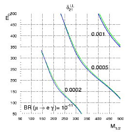
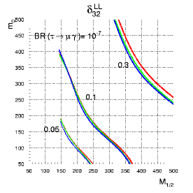
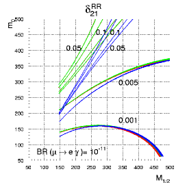
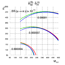
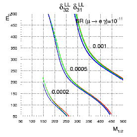
In fig.1 we can see the bounds on and
coming from and ,
respectively.
As for , the limit on is such that
.
The red lines correspond to the full computations while the green and the blue
lines refer to the mass insertion (MI) and to the generalized mass insertion (GMI)
approximations, respectively.
In the case, MI and full computations give indistinguishable results
and the GMI gives a very satisfactory approximation (see the next section for a quantitative
estimate). In the case the degree of approximation is worse than in the
case. The motivation is that the flavour violating (FV) and conserving (FC)
insertions of the sector are generally larger than those relative
to the sector. For instance, and
.
A large FV insertion, as for , produces a sizable distinction
between approximated and full computations as it must be when we go away from
the perturbative region.
The effect of a large FC insertion is evident
for small , where the term is much larger than the slepton masses,
so that to treat as insertion is not
properly correct.
In fig. 1, the most appreciable deviations between the full computation
and the GMI one are due to the approximations in the neutralino mixing
and they tend to vanish in the large limit,
where the neutralino (chargino) mass matrix expansion is better justified.
We remark that we don’t see these deviations
in the regions with chargino or pure-Bino dominance (in fact these last
contributions are lesser affected by the GMI approximations).
The bounds are rather insensitive to the sign of .
 |
 |
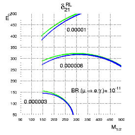
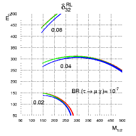
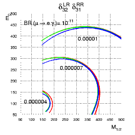
6.2 Bounds on
In this case, the only contribution arises from the exchange
and the amplitude does not contain a factor so bound
is independent, unlike all the other bounds.
In the GMI approximation, the amplitude has the following expression:
We note that the chirality flip is realized directly by the mass insertion so
we can understand the order of the bound, compared to the case,
,
as confirmed numerically.
While MI and full computations give practically the same result both in
and in sectors, the GMI approximation starts to work very well when .
This result can be better understood by bearing in mind the
conditions under which the GMI approximation can be applied.
A necessary condition is that which is not satisfied
when .
In the case we did not have this problem because of the chargino dominance.
We remind that so we would expect the same behavior when
but this region is forbidden by the LSP Bino constraint.
In the sector, both MI and GMI approximations show a sizable deviation from
the full computation in small regions because of a large .
A large induces a mass split of order
in the third generation so, in the mass insertion language,
we are neglecting next to leading terms of order
not so suppressed in the examined case.
We note that the same argument holds for the case.
 |
 |
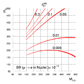
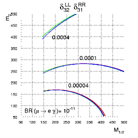
6.3 Bounds on
The sector requires a bit more of attention because of some
cancellations occurring among the amplitudes in some regions of the
parameter space.
The bounds on become very weak so, it is
interesting to check what is limit of applicability
of the mass insertion approximations 222This typically occurs for RR type
MI as long as universality in the gaugino masses is maintained at the high scale.
Although in a completely generic situation without any universal boundary conditions,
such cancellations can occur for LL type MI also [36]..
The origin of this cancellations is the destructive interference between the dominant
contributions coming from the
(with chirality flip implemented through a FC mass insertion)
and exchange.
To better understand the nature of these cancellations
let us derive, in the GMI approximation, the amplitude associated to :
In the above equation, the first term is relative to the pure Bino amplitude with
external chirality flip, the second one corresponds to the mixing in
the neutralino sector while the last term originates from the contribution with
internal sfermion line chirality flip.
It is easy to check numerically that the dominant contributions,
proportional to , have opposite sign in all the parameter space.
To get a feeling of the reason of the above opposite sign, we note that
the amplitude relative to (with chirality flip
implemented through a FC mass insertion) is proportional to with
while the contribution arising from the exchange
is proportional to with (see eqs.3).
Vice-versa, the same type of contributions in the case have the same sign being
proportional to with and
to with , respectively.
The above difference depends on the opposite sign between the hypercharge of
SU(2) doublets and U(1) singlets.
If some cancellations occur among the leading contributions,
subleading effects, generally disregarded, could become important or even dominant.
In this spirit, we retain the amplitude relative to a
chirality flip realized in the external fermion line,
neglected in [14] because it is not enhanced.
Moreover, the above amplitude shows that while the dominant ( enhanced)
contributions are proportional to the mass term
333In reality, this is true only if we neglect the term in
in the pure B amplitude.
the pure amplitude with external chirality flip is independent .
In this way, the branching ratio is not invariant under the change of the sign
so, in general, one has to consider both cases.
In fig. 3 we show the upper limits on from .
The limit on are simply obtained by
thus, by now and are not constrained at all.
As we can see, we are not able to remove these cancellations, in fact, the effect of
the independent contribution is only a shift of the cancellation region
(the same thing happens if we flip the sign).
We remark that, such cancellations occur in all the situations where the contribution of the
term to is negligible.
There are well known model dependent upper bounds on the parameter to avoid
color and e.m. charge breaking, in particular in mSUGRA.
Moreover, mSUGRA requires a large term to fulfill the electroweak symmetry breaking,
thus, we cannot invert the relative sign between the two amplitudes.
In this spirit, we neglected the term in .
It is noteworthy that the MI approximation works very well reproducing the same
cancellation regions as the full computation.
In the GMI case, we have a net shift of this region but the general structure is maintained.
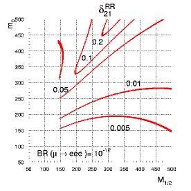
In conclusion, doesn’t allow to put a bound in the sector,
so, we take into account other LFV processes as
and .
As fig. 5 shows, we find that the last process suffers from
a bigger cancellation problem than (in the sector)
while does not.
This result requires some explanations. As we have seen in sec.5, the dominant
contribution to and
arises from the dipole operator (that is enhanced) but, if the dipole
amplitude is strongly suppressed by some cancellations,
goes to zero while and
are dominated by non-dipole contributions.
So, in principle,
and could be able to bound .
As we can see in fig.5, this is the case of that gives a bound for
that is, correctly, independent.
On the other hand, we find that has additional cancellations
between dipole and not-dipole amplitudes.
As a final effect, we have that suffers from
a similar cancellation problem as but,
as can be expected, in a different region of the parameter space.
Because of this strong cancellations, and
prevent us from getting a bound in
the sector both at the present and even in the future when their
experimental sensitivity will be improved.
However, an interesting feature is that and
amplitudes have cancellations in different regions, so, if
we combine the two processes, we obtain a more stringent bound ( 0.2)
than the one coming from ( 0.4).
It is noteworthy that the study of combined processes allows to extract additional
informations respect to each separate case.
 |
 |
 |
 |
6.4 Bounds on the double mass insertion from
As we have seen in the previous section, the bounds on and
are very loose. This is due to a worse experimental resolution
on the above processes compared to the one.
However, we can extract additional information in the and sectors
applying to .
The point is that we are able to put bounds on
the product of two mass insertions, namely .
In general, we can pass from the second to the first generation or
through the or through the insertions.
Now, to constraint the MIs, we proceed exactly as for a single MI.
We put to zero all off diagonal FV entries in the slepton mass matrix except
for the two MIs we are interested to bound.
At this point, we give the analytical expressions for all the type insertions
in the GMI approach.
For we get the following amplitude:
The amplitude , relative to ,
is obtained by .
In fig. 6 we show the bounds on and on
.
As we can see, they exhibit different behaviors,
especially for smaller than due to the and mass difference
(in fact, while in the first case we have two left handed and one right handed sfermions
running in the loop, in the second case we have the opposite situation).
So, while and are indistinguishable,
it is not so for and .
The amplitude associated to ,
namely , reads:
The contribution arising from a type insertion reads:
In the fig. 7 we show the bounds for and for
(equal to the bounds on ).
It is to note that is strongly constrained
because, the associate amplitude, is enhanced respect to the usual
Bino-like mediated processes (being the chirality flip implemented in
the internal sfermion line through
and not by , as usual).
The amplitude , relative to ,
is .
Finally we derive the expression for the amplitude associated to :
We note that, in general, has a bound comparable to , being . The only exception is for () as discussed above.
 |
 |
 |
 |
 |
 |
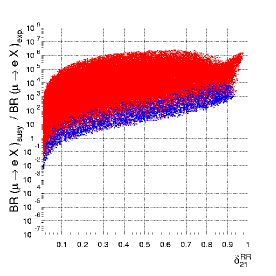
7 Mass eigenstate vs mass insertion: a numerical analysis
At this point, our purpose is to make a quantitative estimate of the goodness of the MI and GMI
approximations.
Even if we have already seen that the above approximations give us the same bounds
as the full computation, we were not able, in the previous analyses, to quantify and
to distinguish correctly the approximations induced by the chargino (neutralino) branch and
by the slepton branch. In the slepton case, we can distinguish between two sources of
approximations, namely, FC and FV terms.
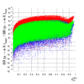
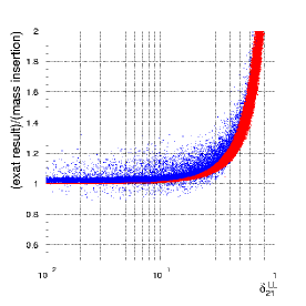
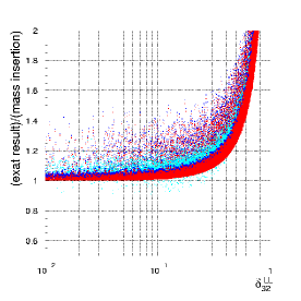
In fig. 8 we show the ratios between full/MI computations (red dots)
and full/GMI computations (blue dots) vs. FV mass insertions.
As we can see in the sector, MI approximates correctly
(at level)
the full computation until large FV insertions (),
while the two computations are practically indistinguishable for .
The induced approximations are easily understood if we remind that the approach we followed
to put the bounds on the insertions was to consider only one mass insertion contributing
at a time for the .
If we stop in the first term we neglect terms of order
in the amplitudes inducing, naively, an approximation on the branching ratios
,
as it is well reproduced numerically. The FC insertion does not produce
any sizable effects, in fact, in the worse case (for large and and
moderate slepton masses), we have .
The last argument is not true in the sector where, being
, we can have a not perturbative
FC insertion. This is clear in fig. 8 where, the MI and the GMI approaches
underline a deviations respect to the exact calculation
(tiny dots refer to the and ,
region where we have sizable deviations due to the slepton FC terms only).
Now, we want to discuss the approximations brought from the chargino and the neutralino sectors
in the GMI approach (the following discussion is obviously flavour independent).
As discussed in section 3, it is allowed to use this method when the elements outside
from the diagonal (proportional to ) are much smaller than those
diagonals ( and ).
On the left of fig. 8, tiny blue dots show a approximation (it happens
in and )
while the much larger ones refer to the and
region where the GMI conditions are fulfilled.
In the case light blue dots correspond to deviations induced by the GMI approximation
in fact they are related to a range of parameters ( and )
where .
To summarize the results found, we can say that MI approximation produce
the same features as the exact calculation even if strong cancellations occur.
The approach works better in the sector than in the one because, while
in the first case we always have perturbative FC terms, in the second case it is not so
and we can reach sizable deviations (up to a level) from the full computation.
Moreover, we have a approximation until FV terms of order 0.2.
The GMI approximation works very well, as the MI approximation, up to gaugino masses
heavier than and it produces the cancellations
in a shifted region respect to the exact case.
In conclusion we can say that, except for fine-tuned cases,
the last approach is very satisfactory.
8 Conclusions
In this work, in the first stage, we studied the constraints on
flavour violating terms in low energy SUSY coming from .
We have carried out the analysis both in the mass eigenstate and in
the mass insertion approximations clarifying the limit of
applicability of these approximations.
In particular, we focused on the RR sector where strong cancellations
make the sector unconstrained.
We showed that these cancellations prevent us from getting a bound in
the sector both at the present and even in the future when the
experimental sensitivity on will be improved.
Finally we took into consideration the bounds on the various double mass insertions:
, ,
, and
.
It is clear that the bounds are approximatively the same as in being
except for the last one suppressed by a factor.
So, in spite of very weak bounds on and on
coming from and respectively, we have stronger bounds on their product thanks
to experimental sensitivity.
These limits are important in order to get the largest amount of information
on SUSY flavour symmetry breaking.
Summarizing the results found in this first stage, we can say that MI approximation produce
the same features as the exact calculation even if strong cancellations occur.
The approach works better in the sector, up to approximation level
until , than in the 32 sector, where, large off
diagonal flavour conserving terms can induce a
deviation from the full computation.
The GMI approximation works very well, as the MI approximation,
except for some special regions where induces a
approximation with respect to the exact calculation and produces the cancellations
in a shift region respect to the exact case. In conclusion, we can say that,
except for fine-tuned cases, the last approach is very satisfactory.
In a second stage, being our aim to find constraints in the
sector, we examined other LFV processes as
and .
We found that the last process suffers from a bigger cancellation problem than
(in the sector) while
does not.
However, an interesting feature is that and
amplitudes have cancellations in different regions, so, if
we combine the two processes, we obtain a more stringent bound ( 0.2)
than the one coming from ( 0.4).
It is noteworthy that the study of combined processes allows to extract additional
information respect to an individual analysis of all these processes.
In particular, it makes it possible to put bounds
on sectors previously unconstrained by .
Acknowledgements
I thank A. Masiero, R. Petronzio, N. Tantalo, S.K. Vempati and O. Vives
for useful discussions.
I also acknowledge the hospitality of the department of physics of Padova,
where part of this work was carried out.
Appendix A Loop functions
In this appendix we report the explicit expressions for the loop functions appearing in the text:
References
- [1] T.C. Cheng and L.F. Li, Phys. Rev. Lett. 45, 1908 (1980); G.Altarelli, L.Baulieu, N.Cabibbo, L.Maiani and R.Petronzio, Nucl.Phys. B 125, 285 (1977); S.T. Petkov, Yad. Fiz. 25, 641 (1977) [Sov. J. Nucl. Phys. 25, 340 (1977)]; A.Sanda, Phys. Lett. 67 B, 303 (1977).
-
[2]
For a recent review, see A. Masiero, S.K. Vempati and O. Vives,
New J.Phys. 6: 202, 2004, arXiv:hep-ph/0407325 and references therein. - [3] P. Minkowski, Phys. Lett. B 67, 421 (1977); T. Yanagida in Proc. Workshop on Unified Theories &c., eds. O. Sawada and A. Sugamoto (Tsukuba, Feb 1979); M. Gell-Mann, P. Ramond, and R. Slansky, in Sanibel Talk , CALT-68-709 (Feb 1979) [arXiv:hep-ph/98090459] (retroprint) and in Supergravity (North Holland Amsterdam, 1979) p. 315; S.L. Glashow, in Quarks and Leptons, Cargèse 1979, eds. M. Lévy, et al., (Plenum 1980 New York), p. 707; R. N. Mohapatra and G. Senjanovic, Phys. Rev. Lett. 44, 912 (1980).
- [4] F. Borzumati and A. Masiero, Phys. Rev. Lett. 57, 961 (1986).
- [5] M. L. Brooks et al. [MEGA Collaboration], Phys. Rev. Lett. 83 (1999) 1521 [arXiv:hep-ex/9905013].
- [6] K. Abe et al. [Belle Collaboration], Phys. Rev. Lett. 92 (2004) 171802 arXiv:hep-ex/0310029.
-
[7]
Y. Yusa, H.Hayashii, T.Nagamine and A.Yamaguchi [Belle Collaboration],
eConf C0209101 (2002) TU13 [Nucl. Phys. Proc. Suppl. 123 (2003) 95]
[arXiv:hep-ex/0211017];
Y. Yusa et al. [Belle Collaboration], Phys. Lett. B589 (2004) 103-110 arXiv:hep-ex/0403039. - [8] K. Aubert et al. [BABAR Collaboration], Phys. Rev. Lett. 92 (2004) 121801 arXiv:hep-ex/0312027; B. Aubert et al. [BABAR Collaboration], Phys. Rev. Lett. 95 (2005) 041802 arXiv:hep-ex/0502032.
- [9] K. Inami, for the Belle Colloboration, Talk presented at the 19th International Workshop on Weak Interactions and Neutrinos (WIN-03) October 6th to 11th, 2003, Lake Geneva, Wisconsin, USA.
- [10] Web page: http://meg.psi.ch
- [11] L. J. Hall, V. A. Kostelecky and S. Raby, Nucl. Phys. B 267, 415 (1986);
- [12] F. Gabbiani and A. Masiero, Nucl. Phys. B 322, 235 (1989).
- [13] F. Gabbiani, E. Gabrielli, A. Masiero and L. Silvestrini, Nucl. Phys. B 477, 321 (1996) [arXiv:hep-ph/9604387].
- [14] I. Masina and C. A. Savoy, Nucl. Phys. B 661, 365 (2003) [arXiv:hep-ph/0211283].
- [15] S. Pokorski, J. Rosiek and C.A.Savoy, Nucl. Phys. B 570, 81 (2000), [arXiv:hep-ph/9906206].
- [16] J. Hisano, T. Moroi, K. Tobe and M. Yamaguchi, Phys. Rev. D 53 (1996) 2442 [arXiv:hep-ph/9510309]; J. Hisano, T. Moroi, K. Tobe and M. Yamaguchi, Phys. Lett. B 391, 341 (1997) [Erratum-ibid. B 397, 357 (1997)] [arXiv:hep-ph/9605296]. J. Hisano, T. Moroi, K. Tobe, M. Yamaguchi and T. Yanagida, Phys. Lett. B 357, 579 (1995) [arXiv:hep-ph/9501407].
- [17] A. Bartl, T. Gajdosik, E. Lunghi, A. Masiero, W. Porod, H. Stremnitzer and O. Vives, Phys. Rev. D 64, 076009 (2001) [arXiv:hep-ph/0103324].
- [18] J. Hisano and D. Nomura, Phys. Rev. D 59, 116005 (1999) [arXiv:hep-ph/9810479].
- [19] An incomplete list of references: S. F. King and I. N. R. Peddie, Nucl. Phys. B 678, 339 (2004) [arXiv:hep-ph/0307091]; J. A. Casas and A. Ibarra, Nucl. Phys. B 618 (2001) 171 [arXiv:hep-ph/0103065]; A. Kageyama, S. Kaneko, N. Shimoyama and M. Tanimoto, Phys. Lett. B 527, 206 (2002) [arXiv:hep-ph/0110283]; F. Deppisch, H. Paes, A. Redelbach, R. Ruckl and Y. Shimizu, Eur. Phys. J. C 28, 365 (2003) [arXiv:hep-ph/0206122]; S. Lavignac, I. Masina and C. A. Savoy, Phys. Lett. B 520, 269 (2001) [arXiv:hep-ph/0106245]; S. Lavignac, I. Masina and C. A. Savoy, Nucl. Phys. B 633, 139 (2002) [arXiv:hep-ph/0202086]; J. R. Ellis, J. Hisano, M. Raidal and Y. Shimizu, Phys. Rev. D 66, 115013 (2002) [arXiv:hep-ph/0206110]. A. Masiero, S. Profumo, S. K. Vempati and C. E. Yaguna, JHEP 0403, 046 (2004) [arXiv:hep-ph/0401138]; K. Tobe, J. D. Wells and T. Yanagida, Phys. Rev. D 69, 035010 (2004) [arXiv:hep-ph/0310148]; L. J. Hall and Y. Nomura, Phys. Rev. D 66, 075004 (2002) [arXiv:hep-ph/0205067]; H. Abe, K. Choi, K. S. Jeong and K. i. Okumura, arXiv:hep-ph/0407005; S. T. Petcov, S. Profumo, Y. Takanishi and C. E. Yaguna, Nucl. Phys. B 676, 453 (2004) [arXiv:hep-ph/0306195]; W. Buchmuller, D. Delepine and F. Vissani, Phys. Lett. B 459, 171 (1999) [arXiv:hep-ph/9904219]; W. Buchmuller, D. Delepine, L.T. Handoko Nucl. Phys. B 576,445 (2000) [arXiv:hep-ph/9912317]; J. R. Ellis and M. Raidal, Nucl. Phys. B 643, 229 (2002) [arXiv:hep-ph/0206174]; S. Pascoli, S. T. Petcov and W. Rodejohann, Phys. Rev. D 68, 093007 (2003) [arXiv:hep-ph/0302054]; K. S. Babu, B. Dutta and R. N. Mohapatra, Phys. Rev. D 67, 076006 (2003) [arXiv:hep-ph/0211068]; J. Sato, K. Tobe and T. Yanagida, Phys. Lett. B 498, 189 (2001) [arXiv:hep-ph/0010348]; T. Blazek and S. F. King, Phys. Lett. B 518, 109 (2001) [arXiv:hep-ph/0105005]; J. I. Illana and M. Masip, Eur. Phys. J. C 35, 365 (2004) [arXiv:hep-ph/0307393]; S. F. King and M. Oliveira, Phys. Rev. D 60, 035003 (1999) [arXiv:hep-ph/9804283]; J. L. Feng, Y. Nir and Y. Shadmi, Phys. Rev. D 61, 113005 (2000) [arXiv:hep-ph/9911370]; J. R. Ellis, M. E. Gomez, G. K. Leontaris, S. Lola and D. V. Nanopoulos, Eur. Phys. J. C 14, 319 (2000) [arXiv:hep-ph/9911459]; D. F. Carvalho, J. R. Ellis, M. E. Gomez and S. Lola, Phys. Lett. B 515, 323 (2001) [arXiv:hep-ph/0103256]; J. Sato and K. Tobe, Phys. Rev. D 63, 116010 (2001) [arXiv:hep-ph/0012333]; J. I. Illana and M. Masip, Phys. Rev. D 67, 035004 (2003) [arXiv:hep-ph/0207328]; J. Cao, Z. Xiong and J. M. Yang, Eur. Phys. J. C 32 (2004) 245 [arXiv:hep-ph/0307126]; A. Rossi, Phys. Rev. D 66, 075003 (2002) [arXiv:hep-ph/0207006]; A. Brignole, A. Rossi, Nucl. Phys. B 587, (2000) 3 [arXiv:hep-ph/0006036].
- [20] For a study of LFV at future colliders, see for example: N. Arkani-Hamed, H. C. Cheng, J. L. Feng and L. J. Hall, Phys. Rev. Lett. 77, 1937 (1996) [arXiv:hep-ph/9603431]; J. Hisano, M. M. Nojiri, Y. Shimizu and M. Tanaka, Phys. Rev. D 60, 055008 (1999) [arXiv:hep-ph/9808410]; F. Deppisch, H. Pas, A. Redelbach, R. Ruckl and Y. Shimizu, Phys. Rev. D 69, 054014 (2004) [arXiv:hep-ph/0310053]; M. Cannoni, S. Kolb and O. Panella, Phys. Rev. D 68, 096002 (2003) [arXiv:hep-ph/0306170]; S. N. Gninenko, M. M. Kirsanov, N. V. Krasnikov and V. A. Matveev, Mod. Phys. Lett. A 17, 1407 (2002) [arXiv:hep-ph/0106302]; M. Sher and I. Turan, Phys. Rev. D 69, 017302 (2004) [arXiv:hep-ph/0309183]; S. Kanemura, Y. Kuno, M. Kuze and T. Ota, Phys. Lett. B 607, 165 (2005) [arXiv:hep-ph/0410044].
- [21] For a recent review, see A. Masiero and O. Vives, Ann. Rev. Nucl. Part. Sci. 51 (2001) 161 [arXiv:hep-ph/0104027]; A. Masiero and O. Vives, New Jour. Phys. 4 (2002) 4.
- [22] For a recent review, please see D. J. H. Chung, L. L. Everett, G. L. Kane, S. F. King, J. Lykken and L. T. Wang, arXiv:hep-ph/0312378.
- [23] R. Barbieri and L. J. Hall, Phys. Lett. B 338, 212 (1994) [arXiv:hep-ph/9408406]; R. Barbieri, L. J. Hall and A. Strumia, Nucl. Phys. B 445, 219 (1995) [arXiv:hep-ph/9501334].
- [24] A. Masiero, S. K. Vempati and O. Vives, Nucl. Phys. B 649, 189 (2003) [arXiv:hep-ph/0209303]; arXiv:hep-ph/0405017.
- [25] See for example, A. Brignole, L. E. Ibanez and C. Munoz, arXiv:hep-ph/9707209 and references therein.
- [26] E. Dudas, S. Pokorski and C. A. Savoy, Phys. Lett. B 369, 255 (1996) [arXiv:hep-ph/9509410].
- [27] S. A. Abel and G. Servant, Nucl. Phys. B 611, 43 (2001) [arXiv:hep-ph/0105262]; G. G. Ross and O. Vives, Phys. Rev. D 67, 095013 (2003) [arXiv:hep-ph/0211279].
- [28] S. F. King, I. N. R. Peddie, G. G. Ross, L. Velasco-Sevilla and O. Vives, arXiv:hep-ph/0407012.
- [29] See for example, R. Kitano, M. Koike and Y. Okada, Phys. Rev. D 66, 096002 (2002) [arXiv:hep-ph/0203110]; R. Kitano, M. Koike, S. Komine and Y. Okada, Phys. Lett. B 575, 300 (2003) [arXiv:hep-ph/0308021] and references therein.
- [30] K. S. Babu and C. Kolda, Phys. Rev. Lett. 89, 241802 (2002) [arXiv:hep-ph/0206310]; A. Dedes, J. R. Ellis and M. Raidal, Phys. Lett. B 549, 159 (2002) [arXiv:hep-ph/0209207].
- [31] M. Sher, Phys. Rev. D 66, 057301 (2002) [arXiv:hep-ph/0207136].
- [32] For a comprehensive analysis of phenomenology, please see: A. Brignole and A. Rossi, Nucl. Phys. B 701, 3 (2004) [arXiv:hep-ph/0404211]; A. Brignole and A. Rossi, Phys. Lett. B 566, 217 (2003) [arXiv:hep-ph/0304081].
- [33] P. Paradisi, arXiv:hep-ph/0508054.
- [34] M. Ciuchini, A. Masiero, L. Silvestrini, S. K. Vempati and O. Vives, Phys. Rev. Lett. 92, 071801 (2004) [arXiv:hep-ph/0307191].
- [35] M. Ciuchini, A. Masiero, P. Paradisi, L. Silvestrini, S. K. Vempati and O. Vives, to appear.
- [36] See for example, S. Profumo and C. E. Yaguna, Nucl. Phys. B 681, 247 (2004) [arXiv:hep-ph/0307225].