SLAC–PUB–11154 hep-ph/0505037

Dijet Event Shapes as Diagnostic Tools

Carola F. Berger

Stanford Linear Accelerator Center
Stanford University, Stanford, California 94309, USA

ABSTRACT

Event shapes have long been used to extract information about hadronic final states and the properties of QCD, such as particle spin and the running coupling. Recently, a family of event shapes, the angularities, has been introduced that depends on a continuous parameter. This additional parameter-dependence further extends the versatility of event shapes. It provides a handle on nonperturbative power corrections, on non-global logarithms, and on the flow of color in the final state.

1 Introduction

Event shapes are generalizations of jet cross sections that describe the distribution of radiation in the final state. Because no individual hadrons are observed, event shapes are infrared-safe. This renders the main features of event shapes, which are determined by the underlying hard scattering, perturbatively calculable (for recent summaries see Refs. [1, 2]). Event shape observables are therefore an ideal testing ground of QCD. For example, they allow the determination of the gluon spin [3], of QCD color factors [4], and precise measurements of the running coupling [5].

Nevertheless, event shape observables retain sensitivity to long-distance hadronization effects. For average values of $e^{+}e^{-}$ event shapes, these nonperturbative corrections manifest themselves as more-or-less additive corrections, typically proportional to the inverse power of the center-of-mass (c.m.) energy, $1/Q$. Differential distributions, which give important additional information about the dynamics of QCD, however, require a more involved convolution with functions that parameterize hadronization effects (for reviews see for example Refs. [1, 6]).

Below we will illustrate how the introduction of a parameter-dependence into an event shape observable can considerably extend the information that can be extracted from its measurement. We discuss a set of event shapes, the so-called class of angularities [7, 8, 9], that depends on a continuous real parameter. This parameter-dependence allows to test nonperturbative features of event shape distributions [10], to control large non-global logarithmic corrections [7, 8], and, in the case of hadronic collisions, to obtain information about the underlying color flow [11].

We begin with a necessarily incomplete review of a prominent event shape, the thrust [12, 13], and introduce the family of angularities. We then derive the scaling rule for nonperturbative power corrections to distributions of angularities. Next, we illustrate how the correlation of angularities with non-global observables, that is, with observables that are designed to measure radiation into only part of phase space, can be used to dampen the sensitivity of the perturbative calculation to soft-gluon radiation at wide angles away from the point of interest. In Section 5 we propose an extension of the definition of angularities to hadronic collisions, and show how such an observable may be used to extract information about the distribution of color in the underlying hard scattering. We end with a summary and point out future directions.

2 The Thrust and Its Extension to the Family of Angularities

2.1 Determination of Gluon Spin via the Thrust

One of the prime examples of an event shape observable in $e^{+}e^{-}$ collisions is the thrust [12, 13] T:

$$T=\frac{1}{\sum\limits_{j\in N}\left|\vec{p}_{j}\right|}\max_{\hat{n}}\sum\limits_{i\in N}\left|\vec{p}_{i}\cdot\hat{n}\right|\,,$$ (1)

where the sums are over all particles in the final state $N$, and $\hat{n}$ is a unit vector whose direction is called the thrust axis when $T$ is maximal. For massless partons, this definition can be written equivalently as

$$\tau\equiv 1-T=\frac{1}{Q}\sum_{i\in N}\ p_{\perp,i}\;e^{-|\eta_{i}|}\,,$$ (2)

where $p_{\perp,i}$ and $\eta_{i}$ denote the transverse momentum and pseudorapidity $\eta_{i}=\ln\cot(\theta_{i}/2)$, respectively, of particle $i$, with respect to the thrust axis. The maximization is implied. Here and below, we treat all partons as massless, parton masses induce corrections which have been examined in Ref. [14].

The thrust measures how pencil-like a particular event is. In the limit of two back-to-back jets, the value of $T$ is 1, whereas its minimum value of 1/2 corresponds to a completely homogeneous spherical event. Radiative corrections shift the value of the lowest order cross section away from $T=1$. The distribution of radiation, and thus the differential cross section $d\sigma/dT$, depends on the spin of the radiated partons. The first-order QCD cross section is given by

$$\frac{1}{\sigma_{\mbox{\tiny tot}}}\frac{d\sigma(q\bar{q}g)}{dT}=\frac{2\alpha_{s}}{3\pi}\Bigg{[}\frac{2(3T^{2}-3T+2)}{T(1-T)}\ln\left(\frac{2T-1}{1-T}\right)-\frac{3(3T-2)(2-T)}{1-T}\Bigg{]}\,,$$ (3)

whereas the corresponding cross section where a scalar “gluon” is radiated gives a distinctly different distribution,

$$\frac{1}{\sigma_{\mbox{\tiny tot}}}\frac{d\sigma(q\bar{q}S)}{dT}=\frac{\tilde{\alpha}_{s}}{3\pi}\Bigg{[}2\ln\left(\frac{2T-1}{1-T}\right)+\frac{(4-3T)(3T-2)}{1-T}\Bigg{]}\,.$$ (4)

This sensitivity to the spin of the radiated partons was used as one of the first tests of QCD [3]. The definitions of a multitude of other $e^{+}e^{-}$ event shapes measuring various aspects of angular distributions in the final state can be found, for example, in Ref. [1].

2.2 The Family of Angularities

We now extend the definition of the thrust, Eq. (4), by introducing a dependence on a continuous, real parameter $a$, which allows us to study a whole class of event shapes simultaneously. We define the family of angularities by weighing the final state with the function [7, 8, 9]

$$\tau_{a}(N)={1\over Q}\sum_{i\in N}\ p_{\perp,i}\;e^{-|\eta_{i}|{(1-a)}}\,\,,$$ (5)

where the direction of particle $i$ is again measured relative to the thrust axis. The parameter $a$ varies between $a=2$ (the weight function (5) then selects two infinitely narrow, back-to-back jets) and $a=-\infty$ (the fully inclusive limit). The value $a=0$ corresponds to $1-T$, with $T$ the thrust (1), and $a=1$ corresponds to the jet broadening [15].

In the two-jet limit, $\tau_{a}$ approaches $0$, and the differential cross section $d\sigma/d\tau_{a}$ receives large corrections in $\ln\left(1/\tau_{a}\right)$ due to soft gluon radiation which have to be resummed for a reliable theoretical prediction. This resummation has been performed to all logarithmic orders at leading power for $a<1$ in Ref. [8]. For $a\sim 1$, recoil effects have to be taken into account, as was pointed out for the broadening ($a=1$) in Ref. [16]. All equations below are therefore valid in the range $a<1$, where the value of $a$ is not too close to 1.

We quote the result of the resummation of large logarithms of $\tau_{a}$ in Laplace moment space:

$$\tilde{\sigma}\left(\nu,Q,a\right)=\int^{\infty}_{0}d\tau_{a}\,{\rm e}^{\;-\nu\,\tau_{a}}\ {d\sigma(\tau_{a},Q)\over d\tau_{a}}\,.$$ (6)

Logarithms of $1/\tau_{a}$ are transformed into logarithms of $\nu$. At next-to-leading logarithmic (NLL) order, we find

$${1\over\sigma_{\rm tot}}\,\tilde{\sigma}\left(\nu,Q,a\right) = \exp\Bigg{\{}2\,\int\limits_{0}^{1}\frac{du}{u}\Bigg{[}\,\int\limits_{u^{2}Q^{2}}^{uQ^{2}}\frac{dp_{\perp}^{2}}{p_{\perp}^{2}}A\left(\alpha_{s}(p_{\perp})\right)\left({\rm e}^{-u^{1-a}\nu\left(p_{\perp}/Q\right)^{a}}-1\right)$$ (7)

$$\qquad\quad\qquad\qquad+\,\frac{1}{2}B\left(\alpha_{s}(\sqrt{u}Q)\right)\left({\rm e}^{-u\left(\nu/2\right)^{2/(2-a)}}-1\right)\Bigg{]}\Bigg{\}}.$$

We see that for small $\tau_{a}$, the cross section factorizes into contributions from two independently radiating jets, resulting in the Sudakov exponent above, where the factor of two stems from the two equal jet contributions. Here, $A(\alpha_{s})$ and $B(\alpha_{s})$ are well-known anomalous dimensions that are independent of $a$. They have finite expansions in the running coupling, $A(\alpha_{s})=\sum_{n=1}^{\infty}A^{(n)}\ (\alpha_{s}/\pi)^{n}$, and similarly for $B(\alpha_{s})$, with the coefficients $A^{(1)}=C_{F},\,B^{(1)}=-3/2\,C_{F},\,A^{(2)}=1/2\,C_{F}[C_{A}(67/18-\pi^{2}/6)-10/9\,T_{F}N_{f}]$, at NLL accuracy, with the color factors $C_{F}=4/3$, $C_{A}=3$, $T_{F}=1/2$, and $N_{f}$ denotes the number of flavors. At $a=0$ we reproduce the NLL resummed thrust cross section [17]. The explicit NLL expression in transform space can be found in Ref. [10], and a formula for the resummed cross section valid to all logarithmic orders at leading power is given in Ref. [8].

3 Universality of Power Corrections

As already mentioned in the introduction, the resummed expression (7) is plagued by sensitivity to long-distance effects. This sensitivity manifests itself as an ambiguity in how to deal with the not well-defined integral over the running coupling, and the validity of the perturbative approach breaks down at $\tau_{a}\sim\Lambda_{\mbox{\tiny QCD}}/Q$. There exist a variety of approaches (see for example Ref. [6]), but in all cases one has to supplement the perturbative calculation with additional information. In the present case, as we will see below, the knowledge of nonperturbative (NP) corrections for only one specific value of $a$ suffices to determine unambiguously the full distribution, including power corrections, for all other values of $a$ ($a<1$).

Due to the quantum mechanical incoherence of short- and long-distance effects, we can separate the perturbative part from the NP contribution in a well-defined, although prescription-dependent manner. Following Refs. [18, 19], we deduce the structure of the NP corrections by a direct expansion of the integrand in the exponent at momentum scales below an infrared factorization scale $\kappa$. We rewrite Eq. (7) as the sum of a perturbative term, labelled with the subscript PT, where all $p_{\perp}>\kappa$, and a soft term that contains all NP physics:

$$\ln\left[\frac{1}{\sigma_{\mbox{\tiny tot}}}\tilde{\sigma}\left(\nu,Q,a\right)\right] = \!\!2\left[\int\limits_{\kappa^{2}}^{Q^{2}}\frac{dp_{\perp}^{2}}{p_{\perp}^{2}}+\int\limits_{0}^{\kappa^{2}}\frac{dp_{\perp}^{2}}{p_{\perp}^{2}}\right]A\left(\alpha_{s}(p_{\perp})\right)\!\!\!\!\!\int\limits_{p_{\perp}^{2}/Q^{2}}^{p_{\perp}/Q}\!\!\frac{du}{u}\left(e^{-u^{1-a}\nu\left(p_{\perp}/Q\right)^{a}}-1\right)$$ (8)

$$\qquad+\,B\mbox{-term}$$

$$\equiv \ln\left[\frac{1}{\sigma_{\mbox{\tiny tot}}}\tilde{\sigma}_{\mbox{\tiny PT}}\left(\nu,Q,\kappa,a\right)\right]$$

$$\qquad\qquad+\frac{2}{1-a}\sum\limits_{n=1}^{\infty}\frac{1}{n\,n!}\left(-\frac{\nu}{Q}\right)^{n}\int\limits_{0}^{\kappa^{2}}\frac{dp_{\perp}^{2}}{p_{\perp}^{2}}p_{\perp}^{n}A\left(\alpha_{s}(p_{\perp})\right).$$

We have suppressed terms of order ${\mathcal{O}}(\nu/Q^{2-a},\nu^{\frac{2}{2-a}}/Q^{2})$, which include the entire $B$-term of Eq. (7), as indicated. Introducing the shape function as an expansion in powers of $\nu/Q$, from the expansion of the exponent in the second equality of (8), with NP coefficients $\lambda_{n}(\kappa)$, we arrive at,

$$\tilde{\sigma}\left(\nu,Q,a\right) = \tilde{\sigma}_{\mbox{\tiny PT}}\left(\nu,Q,\kappa,a\right)\,\tilde{f}_{a,\mbox{\tiny NP}}\left(\frac{\nu}{Q},\kappa\right),\,\,\,$$ (9)

$$\ln\tilde{f}_{a,\mbox{\tiny NP}}\left(\frac{\nu}{Q},\kappa\right) \equiv \frac{1}{1-a}\sum\limits_{n=1}^{\infty}\lambda_{n}(\kappa)\left(-\frac{\nu}{Q}\right)^{n}.$$ (10)

We find the simple result that the only dependence on $a$ is through an overall factor $1/(1-a)$ which leads to the scaling rule for the shape function [10]:

$$\tilde{f}_{a,\mbox{\tiny NP}}\left(\frac{\nu}{Q},\kappa\right)=\left[\tilde{f}_{0,\mbox{\tiny NP}}\left(\frac{\nu}{Q},\kappa\right)\right]^{\frac{1}{1-a}}.$$ (11)

For example, given the shape function for the thrust, $a=0$, at a specific c.m. energy $Q$, one can predict the shape function and thus from Eq. (9) the complete cross section including all leading power corrections for any other value of $a$.

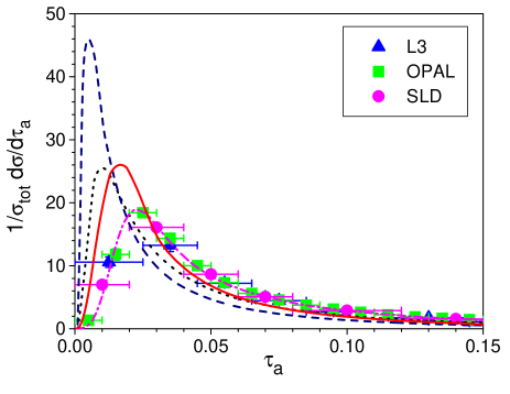
Figure 1: Differential distributions $(1/\sigma_{\mbox{\tiny tot}})d\sigma/d\tau_{a}$ for $a=0$, and $a=-0.5$ at $Q=91$ GeV. Dash-dotted line: output of PYTHIA, $a=0$; dotted line: perturbative contribution at NLL/NLO, $a=0$, as defined in Eq. (8); dashed line: same as dotted line, at $a=-0.5$; solid line: prediction for $a=-0.5$ using Eqs. (9) and (11). The data are taken from Refs. [25, 26, 27].

This is illustrated in Fig. 1, where we plot the differential distributions for the thrust ($a=0$) and for angularity $a=-0.5$. The dotted ($a=0$) and dashed ($a=-0.5$) lines are the theoretical predictions at NLL from Eq. (7) matched to fixed next-to-leading order (NLO) calculations with EVENT2 [23]. In order to compute the shape function via Eq. (9) for $a=0$, we use PYTHIA’s [24] output at $a=0$ (dash-dotted line), instead of fitting a function to the thrust data, since PYTHIA fits these data very well. The prediction for the full differential distribution for $a=-0.5$ (solid line) is then found via (9) and (11) from the so determined shape function and the NLL/NLO computation (dashed line).

The above derivation rests on two main assumptions: Our starting point, the NLL resummed cross section (7), describes independent radiation from the two primary outgoing partons. Inter-hemisphere correlations are neglected, although they are present in the resummed formula valid to all logarithmic orders [8]. However, it has been found from numerical studies that such correlations may indeed be unimportant [20, 21, 22]. Furthermore, we assume in the separation of perturbative and NP effects (8), that long-distance physics has the same properties under boosts as the short-distance radiation. Success or failure of the scaling (11) would thus provide information about these properties of long-distance dynamics.

4 Non-Global Logarithms

The parameter-dependence of the family of angularities can also help to control the sensitivity to wide-angle soft gluon radiation of certain less inclusive, but still infrared safe, so-called non-global, observables.

4.1 Non-Global Observables

Non-global observables measure the radiation into only part of phase space, an example is the energy flow into interjet regions [11, 28]. However, these observables retain sensitivity to radiation away from the location of interest via secondary radiation, as shown in Fig. 2 [29, 30, 31]. Fig. 2 illustrates an energy flow observable associated with radiation into a chosen interjet angular region, $\Omega$ with the complement of $\Omega$ denoted by $\bar{\Omega}$. We are interested in the distribution of $Q_{\Omega}$ for events with a fixed number of jets in $\bar{\Omega}$,

$$A+B\rightarrow\mbox{ Jets }+X_{\bar{\Omega}}+R_{\Omega}(Q_{\Omega})\,.$$ (12)

Here $X_{\bar{\Omega}}$ stands for radiation into the regions between $\Omega$ and the jet axes, and $R_{\Omega}$ for radiation into $\Omega$.

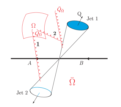
Figure 2: Sources of global and non-global logarithms in dijet events. Configuration 1, a primary emission, is the source of global logarithms, configuration 2 results in non-global logarithms.

As shown in Fig. 2, for these kinds of observables there are two main sources of large logarithmic corrections: “primary” emissions, such as gluon 1 in Fig. 2, are emitted directly from the hard partons into $\Omega$. Phase space integrals for these emissions contribute single logarithms per loop, of order $\alpha_{s}^{n}\ln^{n}(Q/Q_{\Omega})\equiv\alpha_{s}^{n}\ln^{n}1/\varepsilon$, where we have introduced the variable $\varepsilon=Q_{\Omega}/Q$. These logarithms exponentiate as above, (7), and may be resummed in a straightforward fashion [7]. There are also “secondary” emissions originating from the complementary region $\bar{\Omega}$, illustrated by configuration 2 in Fig. 2. As emphasized in Refs. [29, 30], emissions into $\Omega$ from such secondary partons can give logarithms of the form $\alpha_{s}^{n}\ln^{n}(\bar{Q}_{\bar{\Omega}}/Q_{\Omega})$, where $\bar{Q}_{\bar{\Omega}}$ is the maximum energy of radiation in $\bar{\Omega}$. These have become known as non-global logarithms. If no restriction is placed on the radiation into $\bar{\Omega}$, then $\bar{Q}_{\bar{\Omega}}$ can approach $Q$, and the non-global, secondary logarithms can become as important as the primary logarithms. The non-global logarithms arise because real and virtual enhancements associated with secondary emissions do not cancel each other fully at fixed $Q_{\Omega}$, or equivalently $\varepsilon$.

Such non-global logarithms cannot be factorized into a fixed number of jets as in Eq. (7), and therefore do not exponentiate straightforwardly. However, it was found in Ref. [32] that in the limit of large numbers of colors the radiative corrections to non-global energy flow observables can be described by a non-linear evolution equation, which is formally equal to the Kovchegov equation that describes the high-energy behavior of the $S$-matrix [33]. Moreover, for a specific non-global observable, the heavy-quark multiplicity in a certain region of phase space, the non-global evolution linearizes [34, 35] and becomes formally equal to the BFKL equation [36, 37].

4.2 Event Shape/Energy Flow Correlations

An alternative to resumming the secondary logarithms numerically or analytically in the limit or large numbers of colors, is to limit the radiation into the secondary part of phase space by studying correlations between the non-global logarithms and another global observable. Thus “mini-jets” of high energy $\bar{Q}_{\bar{\Omega}}\rightarrow Q$ are suppressed, because the radiation into $\bar{\Omega}$ is now restricted by the value of the global observable. If the global observable in addition has an adjustable parameter, such as the family of angularities, Eq. (5), the importance of the non-global components relative to the primary energy flow can be controlled.

To be specific, we discuss the energy flow/event shape correlations for dijet events in $e^{+}e^{-}$ annihilation where color flow does not add extra complications. We will discuss color flow in hadronic collisions in the next section. We measure the energy flow into $\Omega$ by weighing the final state $N$ with

$$\varepsilon(N)={1\over Q}\ \sum_{\hat{n}_{i}\in\Omega}Q_{i}\,,$$ (13)

where $Q_{i}$ denotes the energy of parton $i$ which is emitted into the region of interest, $\Omega$. This is correlated with the event shape (5), measured in $\bar{\Omega}$. Thus the cross section is given by

$${d\bar{\sigma}(\varepsilon,\tau_{a},Q)\over d\varepsilon\,d\tau_{a}}={1\over 2Q^{2}}\ \sum_{N}\;|M(N)|^{2}\,\delta(\varepsilon-\varepsilon(N))\,\delta(\tau_{a}-\tau_{a}(N))$$ (14)

where we sum over all final states $N$ that contribute to the weighted event, and where $M(N)$ denotes the corresponding amplitude for ${\rm e^{+}e^{-}}\rightarrow N$.

4.2.1 Resummation

We are again interested in dijet events, which correspond to the limit of small $\tau_{a}$ and $\varepsilon$, $\tau_{a},\varepsilon\ll 1$. In this limit, as discussed above, the cross section receives large logarithmic corrections in both variables. However, since for the shape/flow correlation all of phase space is taken into account, we can apply standard factorization and resummation techniques [38, 39].

We arrive at the following factorized cross section in convolution form:

$${1\over\sigma_{\rm tot}}\,\frac{d\bar{\sigma}(\varepsilon,\tau_{a},Q)}{d\varepsilon\,d\tau_{a}} = H\left(\frac{Q}{\mu}\right)\int d\tau_{a\,s}\,\bar{S}\left(\frac{\varepsilon Q}{\mu},\frac{\varepsilon}{\tau_{a\,s}},\frac{\tau_{a\,s}Q}{\mu}\right)$$ (15)

$$\times\,\prod_{i=1,2}\int d\tau_{a\,J_{i}}\,\bar{J}_{i}\left(\frac{\tau_{a\,J_{i}}Q}{\mu}\right)\delta\left(\tau_{a}-\tau_{a\,s}-\tau_{a\,J_{1}}-\tau_{a\,J_{2}}\right)\,.\,\,$$

Here, $\mu$ is the factorization scale which we take for simplicity equal to the renomalization scale. $H$ is a short-distance function, where all momenta are far off-shell, of order $Q$. This hard scattering function is therefore independent of the shape/flow correlations, and only depends on the energy (and implicitly on the scattering angles). $\bar{S}$ is a subdiagram that describes soft radiation away from the two jets $\bar{J}_{i}$, which contain all information about radiation collinear to the primary partons, and are thus constrained only by the event shape variable $\tau_{a}$. In contrast, $\bar{S}$ depends on both, the event shape variable $\tau_{a}$, and the wide-angle radiation into $\Omega$ measured via $\varepsilon$. In Laplace transform space the convolution (15) becomes a simple product,

$$\frac{d\sigma\left(\varepsilon,\nu_{a},Q\right)}{d\varepsilon} = \int^{\infty}_{0}d\tau_{a}\,{\rm e}^{\;-\nu_{a}\,\tau_{a}}\ {d\bar{\sigma}(\varepsilon,\tau_{a},Q)\over d\varepsilon\,d\tau_{a}}\,.$$ (16)

$${1\over\sigma_{\rm tot}}\frac{d\sigma\left(\varepsilon,\nu_{a},Q\right)}{d\varepsilon} = H\left(\frac{Q}{\mu}\right)S\left(\frac{\varepsilon Q}{\mu},\varepsilon\nu_{a},\frac{Q}{\nu_{a}\mu}\right)\prod_{i=1,2}J_{i}\left(\frac{Q}{\nu_{a}\mu}\right),$$ (17)

where now the unbarred quantities denote the Laplace transforms of the corresponding functions in (15).

Resummation of the large logarithms in $\varepsilon$ and $\nu_{a}$ is now straightforward. We use the fact that the physical cross section is independent of the factorization scale

$$\mu\frac{d}{d\mu}\left(\frac{d\sigma\left(\varepsilon,\nu_{a},Q\right)}{d\varepsilon}\right)=0$$ (18)

to obtain the following renormalization-group equations for the soft function,

$$\mu\frac{d}{d\mu}\ln S\left(\frac{\varepsilon Q}{\mu},\varepsilon\nu_{a},\frac{Q}{\nu_{a}\mu}\right)=-\gamma_{s}(\alpha_{s}(\mu))\,,$$ (19)

where $\gamma_{s}$ is the soft anomalous dimension. Analogous equations are found for the jet functions. The anomalous dimensions can depend only on variables held in common between at least two of the functions. Because each function is infrared safe, while ultraviolet divergences are present only in virtual diagrams, the anomalous dimensions cannot depend on the parameters $\nu_{a}$, $\varepsilon$ or $a$. This leaves as arguments of the $\gamma$s only the coupling $\alpha_{s}(\mu)$. The solution to Eq. (19) is found easily,

$$S\left(\frac{\varepsilon Q}{\mu},\varepsilon\nu_{a},\frac{Q}{\nu_{a}\mu}\right)=S\left(\frac{\varepsilon Q}{\mu_{0}},\varepsilon\nu_{a},\frac{Q}{\nu_{a}\mu_{0}},a\right)e^{-\int\limits_{\mu_{0}}^{\mu}\frac{d\lambda}{\lambda}\gamma_{s}(\alpha_{s}(\lambda))}.$$ (20)

Choosing $\mu_{0}$ of order $\nu_{a}$ relegates all large logarithms $\ln\nu_{a}$ into the exponent, as desired. By employing further evolution equations and proper choices for the initial scales we achieve exponentiation of all large logarithms $\ln\nu_{a}$ and $\ln\varepsilon$, leaving only logarithms of order $\ln(\varepsilon\nu_{a})$ unexponentiated. For the full, a bit unwieldy final resummed expression and all technical details, we refer to Refs. [8, 40].

To summarize, large logarithms stemming from either the restriction of radiation by the global event shape or by the non-global observable can be resummed by standard techniques into a Sudakov form analogous to Eq. (7), leaving only an unexponentiated piece from soft wide-angle radiation that contributes logarithms of order $\ln(\varepsilon\nu_{a})$, or equivalently, upon transformation back from moment space, of order $\ln(\varepsilon/\tau_{a})$. Moreover, we observe that the not yet fully exponentiated logarithms $\ln(\varepsilon/\tau_{a})$ stem from wide-angle soft radiation that completely decouples from the jets. This soft radiation can be described by functions constructed entirely out of non-abelian phases, or Wilson (eikonal) lines [38]. It is well-known that such eikonal quantities exponentiate directly by a reordering of color factors and with the help of an identity for eikonalized propagators [41, 42]. Therefore all large logarithms, including logarithms of $(\varepsilon/\tau_{a})$ exponentiate, as was also found in Ref. [43] by an alternative analysis via the coherent branching formalism. Furthermore, by choosing a parameter-dependent global event shape we are able to dial the importance of these correlated logarithms $\sim\ln(\varepsilon/\tau_{a})$, and thus study the behavior of the non-global logarithms.

5 Color Flow

Above, we have discussed energy flow observables, which provide information that is in some sense complementary to what we learn from the study of event shapes. Event shapes shed light on the global distribution of radiation, with the main features determined by the underlying hard scattering. Long-distance effects soften these main features, but not drastically so. Interjet energy flow, on the other hand, reflects the interference between radiation from different jets [44], and encodes the mechanisms that neutralize color in the hadronization process. The study of the interplay between energy and color flow in hadronic collisions [45] may therefore help identify the underlying event [46, 47], to distinguish QCD bremsstrahlung from signals of new physics.

5.1 Hadronic Angularities

In order to study color flow we need to define event shape observables suitable for hadronic collisions. Because parton-parton scattering is highly singular in the forward direction, with a $1/\sin^{4}(\theta/2)$ behavior due to gluon exchange, $e^{+}e^{-}$ event shape definitions have to be adapted to accommodate this behavior in the hadronic case. For further discussion of hadronic event shapes we refer to Ref. [2]. Again, the introduction of a parameter-dependent observable allows us to control the aforementioned difficulties.

We propose the following extension of the set of angularities to hadronic collisions [48],

$$\tau_{a}(N)=\frac{1}{\sqrt{s}}\sum\limits_{i\in N}\ p_{\perp,i}\;e^{-|\eta_{i}|{(1-a)}}\,\,,$$ (21)

Here, in contrast to Eq. (5), the transverse momentum $p_{\perp,i}$ and rapidity $\eta_{i}$ of parton $i$ is measured relative to the collision axis in the c.m. frame. The parameter $a$ allows us to control the sensitivity to the forward direction.

The hadronic cross section for the process $A+B\rightarrow\mbox{ Jets }+X$ at c.m. energy $\sqrt{s}$ is now given by a convolution of standard parton distribution functions (PDFs) $\phi_{f/H}$ with a short-distance partonic cross section $d\hat{\sigma}$:

$$\frac{d\sigma_{AB}(\tau_{a},p_{\perp})}{d\eta dp_{\perp}d\tau_{a}} = \sum_{\rm f}\int dx_{A}dx_{B}\;{\phi}_{f_{A}/A}\left(x_{A},\mu_{F}\right){\phi}_{f_{B}/B}\left(x_{B},\mu_{F}\right)\,$$ (22)

$$\qquad\times\,\delta\left(p_{\perp}-{\sqrt{\hat{s}}\over 2\cosh\hat{\eta}}\right)\,\frac{d\hat{\sigma}^{\rm(f)}(\tau_{a},p_{\perp},\mu_{F})}{d\hat{\eta}d\tau_{a}}\,.$$

$\mu_{F}$ denotes the factorization scale. The PDFs $\phi_{f/H}$ describe the probability for finding parton $f$ in hadron $H$ with momentum fraction $x$. Hatted quantities are given in the partonic c.m. frame, which can be found from the corresponding hadronic quantities via $\hat{\eta}=\eta-(1/2)\ln(x_{A}/x_{B})$, and $\hat{s}=x_{A}x_{B}s$. The superscript $(\rm f)$ denotes the Born-level $2\rightarrow 2$ processes,

$${\rm f}:\quad f_{A}+f_{B}\rightarrow f_{1}+f_{2},$$ (23)

and the sum is over all possible processes. The hard scale is set by the transverse momentum of the observed jet, $p_{\perp}$. Corrections to this leading-twist factorization begin in general with powers of $\Lambda_{\mbox{\tiny QCD}}^{2}/p_{\perp}^{2}$ due to multiple scatterings of partons.

As above, the partonic cross section will receive large logarithmic corrections due to gluon radiation. However, in the case of (21), $\tau_{a}\neq 0$ at lowest order, due to the contributions of the outgoing jets (recall that we measure with respect to the beam axis). Thus, we encounter large logarithms of order $\ln\tilde{\tau}_{a}$, $\tilde{\tau}_{a}\equiv\tau_{a}-\sum_{J=1,2}p_{\perp,J}e^{-|\eta_{J}|(1-a)}$, where the sum is over the outgoing jets. In what follows, moments are taken with respect to $\tilde{\tau}_{a}$.

5.2 Color Evolution

The partonic cross section, $d\hat{\sigma}^{\rm(f)}/(d\hat{\eta}d\tau_{a})$ can be refactorized analogous to Eq. (17), but now we have to take the non-trivial color flow due to colored initial-state partons into account. The regions that give leading contributions are as in the previous section a hard scattering, soft, and jet functions, two for the outgoing jets, and two jet functions for the beam jets. The latter jets must be defined to avoid double counting due to the parton distribution functions. Furthermore, care must be taken in the definition of the outgoing jet functions due to the logarithmic enhancement proportional to $\ln\tilde{\tau}_{a}$ instead of $\ln\tau_{a}$. Such definitions are quite non-trivial, and we do not attempt a full treatment here. Instead, we sketch the main features that emerge independently of the particular details of the chosen observable.

As was observed, for example, in Refs. [11, 45, 49], there is no unique way of defining color exchange in a finite amount of time since gluons of any energy, including soft gluons, carry octet color charge. The functions from which we construct the refactorized partonic cross section are therefore described by matrices in the space of possible color exchanges. This is because as the (re)factorization scale changes, gluons that were included in the hard function become soft and vice versa, as illustrated in Fig. 3. Due to intrajet coherence [44], however, the evolution of the jets themselves is independent of the color exchanges. Once a jet is formed, collinear radiation cannot change its color structure. Therefore, the refactorized partonic shape/flow correlation can be written in moment space as

$${d\hat{\sigma}^{\rm(f)}(\nu_{a},p_{\perp},\mu_{F})\over d\hat{\eta}}=H^{\rm(f)}_{LI}(p_{\perp},\hat{\eta},{\mu},\mu_{F})\;S^{\rm(f)}_{IL}(\nu_{a},\hat{\eta},{\mu})\!\prod_{c=A,B,1,2}\!J^{\rm(f)}_{c}(\nu_{a},p_{\perp},\hat{\eta},{\mu},\mu_{F}).$$ (24)

analogous to the corresponding correlation in $e^{+}e^{-}$ events, Eq. (17). Now the hard and soft functions, $H$ and $S$, respectively, are matrices in the space of color flow. Repeated indices in color space, $L,I,$ are summed over. The superscripts $(\rm f)$ label the underlying partonic process, as in (23). For a list of convenient color bases for the various $2\rightarrow 2$ processes see for example Refs. [40, 45]. $\mu$ is a refactorization scale, not necessarily equal to the factorization scale in Eq. (22).

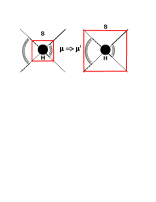
Figure 3: Cartoon illustrating color evolution. $H$ and $S$ are the hard scattering and the soft function, respectively, as described in the text.

The color flow of the event shape is captured by the renormalization-group equation (RGE) that results quite analogously to Eq. (19) from the requirement that the physical cross section be independent of the refactorization scale. Since $H$ and $S$ are matrices in color space, the RGE is now a matrix equation, with anomalous dimension matrices $\Gamma$,

$$\left(\mu\frac{\partial}{\partial\mu}+\beta(g_{s})\frac{\partial}{\partial g_{s}}\right)S_{IL}(\nu_{a},\hat{\eta},{\mu}) = -\left({\Gamma}^{\rm(f)}(\hat{\eta},\alpha_{s}(\mu))\right)^{\dagger}_{IJ}S_{JL}(\nu_{a},\hat{\eta},{\mu})$$ (25)

$$-S_{IJ}(\nu_{a},\hat{\eta},{\mu})\left({\Gamma}^{\rm(f)}(\hat{\eta},\alpha_{s}(\mu))\right)_{JL}\,.$$

Since the anomalous dimension matrices for global event shapes are found as usual from virtual graphs only, the matrices are independent of the shape function and thus universal. They are tabulated in various places, for example in Refs. [40, 45], and have been implemented in the automated resummation program CAESAR [50].

For example, for the computation of the soft anomalous dimension matrix for the partonic subprocess $q_{A}\bar{q}_{B}\rightarrow q_{1}\bar{q}_{2}$ the $t$-channel singlet-octet basis is convenient,

$$c_{1} = \delta_{r_{A},\,r_{1}}\delta_{r_{B},\,r_{2}},$$

$$c_{2} = -\frac{1}{2N_{c}}\delta_{r_{A},\,r_{1}}\delta_{r_{B},\,r_{2}}+\frac{1}{2}\delta_{r_{A},\,r_{B}}\delta_{r_{1},\,r_{2}},\,,$$ (26)

where $r_{i}$ label the color indices of parton $i$, and $N_{c}$ is the number of colors. The soft anomalous dimension matrix in this basis is given by,

$${\Gamma}^{(q\bar{q}\rightarrow q\bar{q})}=\left(\begin{array}[]{cc}2C_{F}T&-\frac{C_{F}}{N_{c}}U\\ -2U&-\frac{1}{N_{c}}(T-2U)\end{array}\right),$$ (27)

where $T$ and $U$ are functions of the Mandelstam variables $\hat{s},\hat{t},\hat{u}$ in the partonic c.m. frame: $T=\ln\left(\frac{-\hat{t}}{\hat{s}}\right)+i\pi,\,U=\ln\left(\frac{-\hat{u}}{\hat{s}}\right)+i\pi$.

The partonic cross section resumming single logarithms in the color flow is then found by solving Eq. (25),

$$\frac{{d\hat{\sigma}}^{\rm(f)}\left(\nu_{a},p_{\perp},\mu_{F})\right)}{d\hat{\eta}} = \prod_{c=A,B,1,2}\!\!\!J^{\rm(f)}_{c}(\nu_{a},p_{\perp},\hat{\eta},{\mu},\mu_{F})$$ (28)

$$\times\sum_{\beta,\,\gamma}\;\!\!\!\!\! \!\!\!H^{\rm(f)}_{\beta\gamma}\left(p_{\perp},\hat{\eta},\mu_{F})\right)\,S^{\rm(f,0)}_{\gamma\beta}\,e^{-\int\limits_{p_{\perp}/\nu_{a}}^{p_{\perp}}\frac{d\lambda}{\lambda}\left[{\lambda}^{\rm(f)\star}_{\gamma}\left(\hat{\eta},\alpha_{s}(\lambda)\right)+{\lambda}^{\rm(f)}_{\beta}\left(\hat{\eta},\alpha_{s}(\lambda)\right)\right]}\,,$$

where we have transformed the matrices $H$ and $S$ to a basis, where the anomalous dimension matrices $\Gamma$ are diagonal.

$$\left(\Gamma_{\mbox{\tiny eik}}^{\rm(f)}(\hat{\eta})\right)_{\gamma\beta}\equiv\lambda^{\rm(f)}_{\beta}(\hat{\eta})\delta_{\gamma\beta}=R^{\rm(f)}_{\gamma I\,}\left(\Gamma_{\mbox{\tiny eik}}^{\rm(f)}(\hat{\eta})\right)_{IJ}\,R^{\rm(f)}{}^{-1}_{J\beta},$$ (29)

with $\lambda^{\rm(f)}_{\beta}$ the eigenvalues of $\Gamma$, and $R$ is the transformation matrix. Greek indices $\beta,\;\gamma$ indicate that a matrix is evaluated in the basis where the eikonal anomalous dimension has been diagonalized.

From Eq. (28) we see that the color flow at NLL is encoded in event shape independent anomalous dimension matrices. It may therefore be possible to find a suitable range of the parameter $a$ in Eq. (21) or perhaps another, different, event shape observable, where small-$x$ effects and problems due to incomplete detector coverage in the forward direction become unimportant, and the study of color flow is unobstructed. Moreover, by combining the analysis of color flow presented above with the study of energy flow discussed in the previous section, as outlined in Ref. [40], we may extract further important information about the dynamics of QCD.

6 Conclusions and Outlook

Above, we have illustrated how the introduction of a parameter-dependence can further increase the amount of information that can be extracted from the study of event shape observables. Aside from information about particle spin and various parameters of QCD, such as color factors and the running coupling, event shapes, especially their distributions, can be used to study the interplay of short- and long-distance dynamics, and obtain insight into the mechanisms of confinement, energy and color flow.

The study of the family of angularities is but a starting point. Given the amount and versatility of event shape observables for processes ranging from electron-positron annihilation over deep inelastic scattering to hadronic collisions, there are many more possibilities and applications. It is certain that continued theoretical and experimental efforts in this direction, at present and future accelerators, will reveal a wealth of information, and probably a few surprises.

References

- [1] M. Dasgupta and G. P. Salam, J. Phys. G 30, R143 (2004) [arXiv:hep-ph/0312283].
- [2] A. Banfi, G. P. Salam and G. Zanderighi, JHEP 0408, 062 (2004) [arXiv:hep-ph/0407287].
- [3] A. De Rujula, J. R. Ellis, E. G. Floratos and M. K. Gaillard, Nucl. Phys. B 138, 387 (1978).
- [4] A. Heister et al. [ALEPH Collaboration], Eur. Phys. J. C 27, 1 (2003).
- [5] S. Bethke, Nucl. Phys. Proc. Suppl. 135, 345 (2004) [arXiv:hep-ex/0407021].
- [6] L. Magnea, On power corrections to event shapes, arXiv:hep-ph/0211013.
- [7] C. F. Berger, T. Kúcs and G. Sterman, Int. J. Mod. Phys. A 18, 4159 (2003) [arXiv:hep-ph/0212343].
- [8] C. F. Berger, T. Kúcs and G. Sterman, Phys. Rev. D 68, 014012 (2003) [arXiv:hep-ph/0303051].
- [9] C. F. Berger and L. Magnea, Phys. Rev. D 70, 094010 (2004) [arXiv:hep-ph/0407024].
- [10] C. F. Berger and G. Sterman, JHEP 0309, 058 (2003) [arXiv:hep-ph/0307394].
- [11] C. F. Berger, T. Kúcs and G. Sterman, Phys. Rev. D 65, 094031 (2002) [arXiv:hep-ph/0110004].
- [12] S. Brandt, C. Peyrou, R. Sosnowski and A. Wroblewski, Phys. Lett. 12, 57 (1964).
- [13] E. Farhi, Phys. Rev. Lett. 39, 1587 (1977).
- [14] G. P. Salam and D. Wicke, JHEP 0105, 061 (2001) [arXiv:hep-ph/0102343].
- [15] S. Catani, G. Turnock and B. R. Webber, Phys. Lett. B 295, 269 (1992).
- [16] Y. L. Dokshitzer, A. Lucenti, G. Marchesini and G. P. Salam, JHEP 9801, 011 (1998) [arXiv:hep-ph/9801324].
- [17] S. Catani, L. Trentadue, G. Turnock and B. R. Webber, Nucl. Phys. B 407, 3 (1993).
- [18] G. P. Korchemsky, in Minneapolis 1998, Continuous advances in QCD, ed. A. V. Smilga (World Scientific, Singapore 1998) 179; arXiv:hep-ph/9806537.
- [19] G. P. Korchemsky and G. Sterman, Nucl. Phys. B 555, 335 (1999) [arXiv:hep-ph/9902341].
- [20] G. P. Korchemsky and S. Tafat, JHEP 0010, 010 (2000) [arXiv:hep-ph/0007005].
- [21] A. V. Belitsky, G. P. Korchemsky and G. Sterman, Phys. Lett. B 515, 297 (2001) [arXiv:hep-ph/0106308].
- [22] E. Gardi and J. Rathsman, Nucl. Phys. B 638, 243 (2002) [arXiv:hep-ph/0201019].
- [23] S. Catani and M. H. Seymour, Phys. Lett. B 378, 287 (1996) [arXiv:hep-ph/9602277].
- [24] T. Sjostrand, P. Eden, C. Friberg, L. Lonnblad, G. Miu, S. Mrenna and E. Norrbin, Comput. Phys. Commun. 135, 238 (2001) [arXiv:hep-ph/0010017].
- [25] B. Adeva et al. [L3 Collaboration], Z. Phys. C 55, 39 (1992).
- [26] P. D. Acton et al. [OPAL Collaboration], Z. Phys. C 59, 1 (1993).
- [27] K. Abe et al. [SLD Collaboration], Phys. Rev. D 51, 962 (1995) [arXiv:hep-ex/9501003].
- [28] N. A. Sveshnikov and F. V. Tkachov, Phys. Lett. B 382, 403 (1996) [arXiv:hep-ph/9512370].
- [29] M. Dasgupta and G. P. Salam, Phys. Lett. B 512, 323 (2001) [arXiv:hep-ph/0104277].
- [30] M. Dasgupta and G. P. Salam, JHEP 0203, 017 (2002) [arXiv:hep-ph/0203009].
- [31] R. B. Appleby and M. H. Seymour, JHEP 0212, 063 (2002) [arXiv:hep-ph/0211426].
- [32] A. Banfi, G. Marchesini and G. Smye, JHEP 0208, 006 (2002) [arXiv:hep-ph/0206076].
- [33] Y. V. Kovchegov, Phys. Rev. D 60, 034008 (1999) [arXiv:hep-ph/9901281].
- [34] G. Marchesini and A. H. Mueller, Phys. Lett. B 575, 37 (2003) [arXiv:hep-ph/0308284].
- [35] G. Marchesini and E. Onofri, JHEP 0407, 031 (2004) [arXiv:hep-ph/0404242].
- [36] E. A. Kuraev, L. N. Lipatov and V. S. Fadin, Sov. Phys. JETP 45, 199 (1977) [Zh. Eksp. Teor. Fiz. 72, 377 (1977)].
- [37] I. I. Balitsky and L. N. Lipatov, Sov. J. Nucl. Phys. 28, 822 (1978) [Yad. Fiz. 28, 1597 (1978)].
- [38] J. C. Collins, D. E. Soper and G. Sterman, Adv. Ser. Direct. High Energy Phys. 5, 1 (1988) [arXiv:hep-ph/0409313].
- [39] G. Sterman, QCD and jets, TASI 2004, arXiv:hep-ph/0412013.
- [40] C. F. Berger, Soft gluon exponentiation and resummation, Ph.D. thesis, SUNY at Stony Brook, 2003, arXiv:hep-ph/0305076.
- [41] G. Sterman, in AIP Conference Proceedings Tallahassee, Perturbative Quantum Chromodynamics, eds. D. W. Duke, J. F. Owens, New York, 1981.
- [42] J. G. M. Gatheral, Phys. Lett. B 133, 90 (1983).
- [43] Y. L. Dokshitzer and G. Marchesini, JHEP 0303, 040 (2003) [arXiv:hep-ph/0303101].
- [44] Y. L. Dokshitzer, V. A. Khoze, S. I. Troian and A. H. Mueller, Rev. Mod. Phys. 60, 373 (1988).
- [45] N. Kidonakis, G. Oderda and G. Sterman, Nucl. Phys. B 531, 365 (1998) [arXiv:hep-ph/9803241].
- [46] P. Skands and T. Sjostrand, Eur. Phys. J. C 33, S548 (2004) [arXiv:hep-ph/0310315].
- [47] D. Acosta et al. [CDF Collaboration], Phys. Rev. D 70, 072002 (2004) [arXiv:hep-ex/0404004].
- [48] G. Sterman, Energy flow observables, arXiv:hep-ph/0501270.
- [49] G. Sterman and M. E. Tejeda-Yeomans, Phys. Lett. B 552, 48 (2003) [arXiv:hep-ph/0210130].
- [50] A. Banfi, G. P. Salam and G. Zanderighi, JHEP 0503, 073 (2005) [arXiv:hep-ph/0407286].
- [51] D. Binosi and L. Theussl, Comput. Phys. Commun. 161, 76 (2004) [arXiv:hep-ph/0309015].
- [52] J. A. M. Vermaseren, Comput. Phys. Commun. 83, 45 (1994).