Static QCD Potential at $r<\Lambda_{\rm QCD}^{-1}$:
Perturbative expansion and operator-product expansion

We analyze the static QCD potential $V_{\rm QCD}(r)$ in the distance region $0.1~{}{\rm fm}\hbox{ \raise 3.0pt\hbox to0.0pt{$<$}\raise-3.0pt\hbox{$\sim$} }r\hbox{ \raise 3.0pt\hbox to0.0pt{$<$}\raise-3.0pt\hbox{$\sim$} }1~{}{\rm fm}$ using perturbative QCD and operator-product expansion (OPE) as basic theoretical tools. We assemble theoretical developments up to date and perform a solid and accurate analysis. The analysis consists of 3 major steps: (I) We study large-order behavior of the perturbative series of $V_{\rm QCD}(r)$ analytically. Higher-order terms are estimated by large-$\beta_{0}$ approximation or by renormalization group, and the renormalization scale is varied around the minimal-sensitivity scale. A “Coulomb”+linear potential can be identified with the scale-independent and renormalon-free part of the prediction and can be separated from the renormalon-dominating part. (II) In the frame of OPE, we define two types of renormalization schemes for the leading Wilson coefficient. One scheme belongs to the class of conventional factorization schemes. The other scheme belongs to a new class, which is independent of the factorization scale, derived from a generalization of the “Coulomb”+linear potential of (I). The Wilson coefficient is free from IR renormalons and IR divergences in both schemes. We study properties of the Wilson coefficient and of the corresponding non-perturbative contribution $\delta E_{\rm US}(r)$ in each scheme. (III) We compare numerically perturbative predictions of the Wilson coefficient and lattice computations of $V_{\rm QCD}(r)$ when $n_{l}=0$. We confirm either correctness or consistency (within uncertainties) of the theoretical predictions made in (II). Then we perform fits to simultaneously determine $\delta E_{\rm US}(r)$ and $r_{0}\Lambda_{\overline{\rm MS}}^{\mbox{\scriptsize 3-loop}}$ (relation between lattice scale and $\Lambda_{\overline{\rm MS}}$). As for the former quantity, we improve bounds as compared to the previous determination; as for the latter quantity, our analysis provides a new method for its determination. We find that (a) $\delta E_{\rm US}(r)=0$ is disfavored, and (b) $r_{0}\Lambda_{\overline{\rm MS}}^{\mbox{\scriptsize 3-loop}}=0.574\pm 0.042$. We elucidate the mechanism for the sensitivities and examine sources of errors in detail.

1 Introduction

In this article, we study the QCD potential for a static quark-antiquark ($Q\bar{Q}$) pair, in the distance region $0.5~{}{\rm GeV}^{-1}\,(0.1~{}{\rm fm})\hbox{ \raise 3.0pt\hbox to0.0pt{$<$}\raise-3.0pt\hbox{$\sim$} }r\hbox{ \raise 3.0pt\hbox to0.0pt{$<$}\raise-3.0pt\hbox{$\sim$} }5~{}{\rm GeV}^{-1}\,(1~{}{\rm fm})$. This region is known to be relevant to the spectroscopy of the heavy quarkonium states. We use perturbative QCD and operator-product-expansion (OPE) as basic theoretical tools, taking advantage of dramatic theoretical developments that took place in the last decade. In addition, we use recent accurate results of lattice computations of the QCD potential.

For 30 years, the static QCD potential $V_{\rm QCD}(r)$ has been studied extensively for the purpose of elucidating the nature of the interaction between heavy quark and antiquark. Generally, $V_{\rm QCD}(r)$ at short-distances can be computed accurately by perturbative QCD. On the other hand, the potential shape at long-distances should be determined by non-perturbative methods, such as lattice simulations or phenomenological potential-model analyses; in the latter approach phenomenological potentials are extracted from experimental data for the heavy quarkonium spectra.

Computations of $V_{\rm QCD}(r)$ in perturbative QCD has a long history. At tree-level, $V_{\rm QCD}(r)$ is merely a Coulomb potential, $-(4/3)(\alpha_{S}/r)$, arising from one-gluon-exchange diagram. The 1-loop correction (with massless internal quarks) was already computed in [1, 2]. The 1-loop correction due to massive internal quarks was computed in [3]. It took a rather long time before the 2-loop correction (with massless internal quarks) was computed in [4]; part of this result was corrected soon in [5]. The 2-loop correction due to massive internal quarks was computed in [6, 7, 8]; misprints in [7, 8] were corrected in [9]. The logarithmic correction at 3-loop originating from the ultrasoft scale was first pointed out in [1] and computed in [10, 11]. A renormalization-group (RG) improvement of $V_{\rm QCD}(r)$ at next-to-next-to-leading logarithmic order (NNLL), including the ultrasoft logarithms, was performed in [12]. (There exist estimates of higher-order corrections to the perturbative QCD potential in various methods [13, 14, 15].)

For a long time, the perturbative QCD predictions of $V_{\rm QCD}(r)$ were not successful in the distance region relevant to the bottomonium and charmonium states, $0.5~{}{\rm GeV}^{-1}\hbox{ \raise 3.0pt\hbox to0.0pt{$<$}\raise-3.0pt\hbox{$\sim$} }r\hbox{ \raise 3.0pt\hbox to0.0pt{$<$}\raise-3.0pt\hbox{$\sim$} }5~{}{\rm GeV}^{-1}$. In fact, the perturbative series turned out to be very poorly convergent at $r\hbox{ \raise 3.0pt\hbox to0.0pt{$>$}\raise-3.0pt\hbox{$\sim$} }0.5~{}{\rm GeV}^{-1}$; uncertainty of the series is so large that one could hardly obtain meaningful prediction in this distance region. Even if one tries to improve the perturbation series by certain resummation prescriptions (such as RG improvement), scheme dependence of the results turns out to be very large; hence, one can neither obtain accurate prediction of the potential in this distance region. For instance, the QCD potential bends downwards at large $r$ as compared to the Coulomb potential if the $V$-scheme running coupling constant is used, whereas the potential bends upwards at large $r$ if the $F$-scheme running coupling constant is used [17]. (See e.g. Fig. 4 of [18].) It was later pointed out that the large uncertainty of the perturbative QCD prediction can be understood as caused by the ${\cal O}(\Lambda_{\rm QCD})$ infrared (IR) renormalon contained in $V_{\rm QCD}(r)$ [19].

Empirically it has been known that phenomenological potentials and lattice computations of $V_{\rm QCD}(r)$ are both approximated well by the sum of a Coulomb potential and a linear potential in the above range $0.5~{}{\rm GeV}^{-1}\hbox{ \raise 3.0pt\hbox to0.0pt{$<$}\raise-3.0pt\hbox{$\sim$} }r\hbox{ \raise 3.0pt\hbox to0.0pt{$<$}\raise-3.0pt\hbox{$\sim$} }5~{}{\rm GeV}^{-1}$ [20]. The linear behavior of $V_{\rm QCD}(r)$ at large distances $r\gg\Lambda_{\rm QCD}^{-1}$, verified numerically by lattice simulations, is consistent with the quark confinement picture. For this reason, and given the very poor predictability of perturbative QCD, it was often said that, while the “Coulomb” part of $V_{\rm QCD}(r)$ (with logarithmic corrections at short-distances) is contained in the perturbative QCD prediction, the linear part is purely non-perturbative and absent in the perturbative QCD prediction (even at $r<\Lambda_{\rm QCD}^{-1}$), and that the linear potential needs to be added to the perturbative prediciton to obtain the full QCD potential. Nevertheless, to the best of our knowledge, there was no firm theoretical basis for this argument.

Since the discovery [21, 22, 23] of the cancellation of ${\cal O}(\Lambda_{\rm QCD})$ renormalons in the total energy of a static quark-antiquark pair $E_{\rm tot}(r)\equiv V_{\rm QCD}(r)+2m_{\rm pole}$, convergence of the perturbative series for $E_{\rm tot}(r)$ improved drastically and much more accurate perturbative predictions for the potential shape became available. It was understood that a large uncertainty originating from the ${\cal O}(\Lambda_{\rm QCD})$ renormalon in $V_{\rm QCD}(r)$ can be absorbed into twice of the quark pole mass $2m_{\rm pole}$. Once this is achieved, perturbative uncertainty of $E_{\rm tot}(r)$ is estimated to be ${\cal O}(\Lambda_{\rm QCD}^{3}r^{2})$ at $r\hbox{ \raise 3.0pt\hbox to0.0pt{$<$}\raise-3.0pt\hbox{$\sim$} }\Lambda_{\rm QCD}^{-1}$ [19], based on the renormalon dominance hypothesis.

On the other hand, OPE of $V_{\rm QCD}(r)$ for $r\ll\Lambda_{\rm QCD}^{-1}$ was developed [10, 24] within an effective field theory “potential non-relativistic QCD” (pNRQCD) [25]. In this framework, $V_{\rm QCD}(r)$ is expanded in $r$ (multipole expansion). At each order of this expansion, short-distance contributions are factorized into Wilson coefficients (perturbatively computable) and long-distance contributions into matrix elements of operators (non-perturbative quantities). The leading non-perturbative contribution to the potential is contained in the ${\cal O}(r^{2})$ term of the multipole expansion.

Subsequently, several studies [18, 9, 26, 27] showed that perturbative predictions for $V_{\rm QCD}(r)$ agree well with phonomenological potentials and lattice calculations of $V_{\rm QCD}(r)$, once the ${\cal O}(\Lambda_{\rm QCD})$ renormalon contained in $V_{\rm QCD}(r)$ is cancelled. In particular, in the context of OPE, the leading Wilson coefficient was shown to be in agreement with lattice computations of $V_{\rm QCD}(r)$, after the subtraction of the ${\cal O}(\Lambda_{\rm QCD})$ renormalon [26]. Ref. [28] showed that a Borel resummation of the perturbative series gives a potential shape which agrees with lattice results, if the ${\cal O}(\Lambda_{\rm QCD})$ renormalon is properly taken into account. In fact, these agreements hold within uncertainties of ${\cal O}(\Lambda_{\rm QCD}^{3}r^{2})$ estimated from the residual renormalon. That is, a linear potential of ${\cal O}(\Lambda_{\rm QCD}^{2}\,r)$ at $r\hbox{ \raise 3.0pt\hbox to0.0pt{$<$}\raise-3.0pt\hbox{$\sim$} }\Lambda_{\rm QCD}^{-1}$ was ruled out numerically in the differences between the perturbative predictions and phenomenological potentials/lattice results. These observations support the validity of renormalon dominance hypothesis.

A crucial point is that, once the ${\cal O}(\Lambda_{\rm QCD})$ renormalon is cancelled and the perturbative prediction is made accurate, the perturbative potential becomes steeper than the Coulomb potential as $r$ increases. This feature is understood, within perturbative QCD, as an effect of the running of the strong coupling constant [29, 18].

Soon after, it was shown analytically [30] that the perturbative QCD potential approaches a “Coulomb”+linear form at large orders, up to an ${\cal O}(\Lambda_{\rm QCD}^{3}r^{2})$ uncertainty. (Here and hereafter, the “Coulomb” potential with quotes represents a Coulombic potential with logarithmic corrections at short distances.) Higher-order terms were estimated by the large-$\beta_{0}$ approximation or by RG equation and a scale-fixing prescription based on renormalon dominance hypothesis was used. The “Coulomb”+linear potential can be computed systematically via RG; up to NNLL, it shows a convergence towards lattice computations of $V_{\rm QCD}(r)$. Furthermore, the “Coulomb”+linear potential was shown to coincide with the leading Wilson coefficient in the framework of OPE, up to an ${\cal O}(r^{2})$ difference [31].

In this paper, we perform a precise and solid analysis, on the basis of our previous works [30, 31]. This work extends our previous works in the following respects:

• We incorporate a degree of freedom for varying renormalization scale into the analysis of [30]. In this way, the “Coulomb”+linear potential is identified with the scale-independent part of the prediction. Details of the derivation and formulas not delivered so far are also presented.

• We promote the “Coulomb”+linear potential to the leading Wilson coefficient in the framework of OPE, taking advantage of the result of [31]. We study properties of the Wilson coefficient and the corresponding non-perturbative correction $\delta E_{\rm US}(r)$.

In addition, we present the following analysis:

• We determine the non-perturbative correction $\delta E_{\rm US}(r)$ using perturbative computations of the Wilson coefficients and recent lattice data.

• As a byproduct, we determine the relation between lattice scale (Sommer scale) and $\Lambda_{\overline{\rm MS}}$. This provides a new method to determine this relation.

In this analysis, we assemble all the developments of perturbative computations and of OPE up to date.

Organization of the paper is as follows. Sec. 2 is devoted to a review: we review the current status of the perturbative QCD computations of $V_{\rm QCD}(r)$ (Sec. 2.1), convergence property of $E_{\rm tot}(r)$ up to ${\cal O}(\alpha_{S}^{3})$ (Sec. 2.2), large-order behavior of the perturbative series based on renormalon argument (Sec. 2.3), and the predictions of OPE for $V_{\rm QCD}(r)$ (Sec. 2.4). In Sec. 3, we analyze the large-order behavior of the perturbative prediction of $V_{\rm QCD}(r)$ analytically: After explaining the strategy in Sec. 3.1, we present the results when the higher-order terms are estimated by the large-$\beta_{0}$ approximation and by RG in Secs. 3.2 and 3.3, respectively. Details of the derivation are given through Secs. 3.4 and 3.5. (The readers may as well skip these details in the first reading.) Sec. 4 defines two types of renormalization schemes for the leading Wilson coefficient in the context of OPE (Secs. 4.1 and 4.2) and discusses properties of the Wilson coefficient and of the corresponding non-perturbative contributions (Sec. 4.3). In Sec. 5 we compare the perturbative computations of the Wilson coefficient with lattice compuations of $V_{\rm QCD}(r)$. We first check consistency of theoretical predictions based on OPE (Sec. 5.1). Then we determine the non-perturbative contribution in each scheme as well as the relation between lattice scale and $\Lambda_{\overline{\rm MS}}$ (Secs. 5.2 and 5.3). Summary and conclusions are given in Sec. 6.

App. A collects the formulas necessary for the computation of the perturbative series of the QCD potential. In App. B, we give a derivation of the one-parameter integral representation of $[\alpha_{V}^{\rm PT}(q)]_{\infty}$. In App. C, we present the analytic formula for the linear potential up to NNLL. Methods for numerical evaluation of the Wilson coefficient are given in App. D.

2 Perturbation Series and OPE of $V_{\rm QCD}(r)$ (Review)

2.1 Definitions and conventions

Throughout this paper, color factors of QCD are denoted as

$$C_{F}=\frac{4}{3},~{}~{}~{}~{}~{}C_{A}=N_{C}=3,~{}~{}~{}~{}~{}T_{F}=\frac{1}{2},$$ (1)

where $N_{C}$ is the number of color, $C_{F}$ is the second Casimir operator of the fundamental representation, $C_{A}$ is the second Casimir operator of the adjoint representation, and $T_{F}$ is the trace normalization of the fundamental representaion of the color $SU(3)$ group. Furthermore, we denote the number of light quark flavors by $n_{l}$. We assume that all light quarks are massless (except in Sec. 2.2).

The static QCD potential is defined from an expectation value of the Wilson loop as

$$V_{\rm QCD}(r) = -\lim_{T\to\infty}\frac{1}{iT}\,\log\frac{\left<{0}\,\right|{\rm{Tr\,P}}\exp\biggl{[}ig_{S}\oint_{\cal P}dx^{\mu}\,A_{\mu}(x)\biggr{]}\left|\,{0}\,\right>}{\left<{0}\,\right|{\rm Tr}\,{\bf 1}\left|\,{0}\,\right>}$$ (2)

$$= \int\frac{d^{d}\vec{q}}{(2\pi)^{d}}\,e^{i\vec{q}\cdot\vec{r}}\,\biggl{[}-4\pi C_{F}\,\frac{\alpha_{V}(q)}{q^{2}}\biggr{]}~{}~{}~{};~{}~{}~{}~{}~{}q=|\vec{q}|,$$ (3)

where ${\cal P}$ is a rectangular loop of spatial extent $r$ and time extent $T$. The second line defines the $V$-scheme coupling contant, $\alpha_{V}(q)$, in momentum space. In dimensional regularization, there are one temporal dimension and $d=D-1=3-2\epsilon$ spatial dimensions.

In perturbative QCD, $\alpha_{V}(q)$ is calculable in series expansion of the strong coupling constant. We denote the perturbative evaluation of $\alpha_{V}(q)$ as

$$\alpha_{V}^{\rm PT}(q) = \alpha_{S}(\mu)\,\sum_{n=0}^{\infty}P_{n}(\log(\mu/q))\,\biggl{(}\frac{\alpha_{S}(\mu)}{4\pi}\biggr{)}^{n}$$ (4)

$$= \alpha_{S}(q)\,\sum_{n=0}^{\infty}P_{n}(0)\,\biggl{(}\frac{\alpha_{S}(q)}{4\pi}\biggr{)}^{n}.$$ (5)

Here, $\alpha_{S}(\mu)$ denotes the strong coupling constant renormalized at the renormalization scale $\mu$, defined in the modified minimal subtraction ($\overline{\rm MS}$) scheme; $P_{n}(\ell)$ denotes an $n$-th-degree polynomial of $\ell$. In the second equality, we set $\mu=q$ using $\mu$-independence of $\alpha_{V}^{\rm PT}(q)$. Eq. (5) is reduced to eq. (4), if we insert the series expansion of $\alpha_{S}(q)$ in terms of $\alpha_{S}(\mu)$. This expansion is determined by the RG equation

$$q^{2}\,\frac{d}{dq^{2}}\,\alpha_{S}(q)=\beta(\alpha_{S}(q))=-\alpha_{S}(q)\sum_{n=-1}^{\infty}\beta_{n}\biggl{(}\frac{\alpha_{S}(q)}{4\pi}\biggr{)}^{n+1},$$ (6)

where $\beta_{n}$ represents the $(n+1)$-loop coefficient of the beta function. Eqs. (4)(5) show that, at each order of the expansion of $\alpha_{V}^{\rm PT}(q)$ in $\alpha_{S}(\mu)$, the only part of the polynomial $P_{n}(\log(\mu/q))$ that is not determined by the RG equation is $P_{n}(0)$.

It is known [1] that $P_{n}(0)$ for $n\geq 3$ contain IR divergences. Namely, the perturbative QCD potential is IR divergent and not well-defined at and beyond ${\cal O}(\alpha_{S}^{4})$. There are two ways to deal with this problem. One way is to use OPE, in which the QCD potential is factorized into Wilson coefficients and matrix elements. The Wilson coefficients include only ultraviolet (UV) contributions, hence they are computable in perturbative expansion in $\alpha_{S}$ free from IR divergences. IR contributions are contained in the matrix elements which are non-perturbative quantities. Another way is to expand the QCD potential as a double series in $\alpha_{S}$ and $\log\alpha_{S}$. This is achieved by resummation of certain class of diagrams (Fig. 1) as indicated by [1]. More systematically, this can be achieved within pNRQCD framework [10, 11, 24]. We will use both methods for regularization of IR divergences through Secs. 3–5.

Figure 1: Class of diagrams contributing to the QCD potential at ${\cal O}(\alpha_{S}^{4}\log\alpha_{S})$. Dashed lines represent Coulomb gluons; curly line represents transverse gluon.

Let us explain our terminology for the order counting. When we state “$\alpha_{V}^{\rm PT}(q)$ up to ${\cal O}(\alpha_{S}^{N})$,” we mean that we truncate the series on the right-hand-side of eq. (4) and take the sum for $0\leq n\leq N\!-\!1$. We also improve the perturbation series using the RG evolution of the $\overline{\rm MS}$ coupling. By $\alpha_{V}^{\rm PT}(q)$ up to LL, NLL, NNLL and NNNLL, we mean that we define $\alpha_{V}^{\rm PT}(q)$ by eqs. (5)(6) and take the sums for $0\leq n\leq 1$, 2, 3 and 4, respectively, in both equations (i.e. 1-, 2-, 3- and 4-loop running coupling constants are used for $\alpha_{S}(q)$, respectively). This procedure resums logarithms of the forms $\alpha_{S}(\mu)[\alpha_{S}(\mu)\log(\mu/q)]^{n}$, $\cdots$, $\alpha_{S}(\mu)^{4}[\alpha_{S}(\mu)\log(\mu/q)]^{n}$, respectively.

On the other hand, the IR divergences at ${\cal O}(\alpha_{S}^{4})$ and beyond induce additional powers of $\log(\mu/q)$ in $\alpha_{V}(q)$ at NNLL and beyond, which are not resummed by the evolution of $\alpha_{S}(q)$ via eq. (6). Hence, at these orders, it is more consistent (with respect to naive power counting) to resum these IR logarithms (referred usually as ultrasoft logarithms) as well, although physical origins of the logarithms are quite different. The ultrasoft (US) logarithms at NNLL can be resummed by replacing the $V$-scheme coupling constant as [12]

$$\alpha_{V}^{\rm PT}(q)\to\alpha_{V}^{\rm PT}(q)+\frac{C_{A}^{3}}{6\beta_{0}}\,\alpha_{S}(q)^{3}\,\log\biggl{[}\frac{\alpha_{S}(q)}{\alpha_{S}(\mu_{f})}\biggr{]},$$ (7)

where $\mu_{f}$ denotes the factorization scale. We will examine the resummation of US logs separately.

For $n\leq 2$, we define $a_{n}\equiv P_{n}(0)$. For $n\geq 3$, we include US logs into $a_{n}$ in addition. Explicit expressions for $P_{n}(\ell)$, $a_{n}$, $\beta_{n}$ up to $n=3$ (except for the unknown part of $a_{3}$) are listed in App. A. Furthermore, for convenience, we will denote

$$\delta={\beta_{1}}/{\beta_{0}^{2}}$$ (8)

in the following. Other formulas, useful for evaluation of $\alpha_{V}^{\rm PT}(q)$, are collected in App. A as well.

2.2 Convergence and scale-dependences of $E_{\rm tot}(r)$ up to ${\cal O}(\alpha_{S}^{3})$

Let us demonstrate the improvement of accuracy of the perturbative prediction for the total energy $E_{\rm tot}(r)=2m_{\rm pole}+V_{\rm QCD}(r)$ up to ${\cal O}(\alpha_{S}^{3})$, when the cancellation of ${\cal O}(\Lambda_{\rm QCD})$ renormalons is incorporated. This is achieved (even without any knowledge of renormalons) if one re-expresses the quark pole mass $m_{\rm pole}$ by the $\overline{\rm MS}$ mass in series expansion in $\alpha_{S}(\mu)$. Presently perturbation series of $V_{\rm QCD}(r)$ [4, 5] and $m_{\rm pole}$ [33] are both known up to ${\cal O}(\alpha_{S}^{3})$.

As an example, we take the bottomonium case: We choose the $\overline{\rm MS}$ mass of the $b$-quark, renormalized at the $b$-quark $\overline{\rm MS}$ mass, as $\overline{m}_{b}\equiv m_{b}^{\overline{\rm MS}}(m_{b}^{\overline{\rm MS}})=4.190$ GeV; in internal loops, four flavors of light quarks are included with $\overline{m}_{u}=\overline{m}_{d}=\overline{m}_{s}=0$ and $\overline{m}_{c}=1.243$ GeV. (See the formula for $E_{{\rm tot}}^{b\bar{b}}(r)$ in [9].) In Fig. 2, we fix $r=2.5~{}{\rm GeV}^{-1}\approx 0.5$ fm (midst of the distance range of our interest) and examine the renormalization scale ($\mu$) dependence of $E_{{\rm tot}}(r)$. We see that $E_{{\rm tot}}(r)$ is much less scale dependent when we use the $\overline{\rm MS}$ mass (after cancellation of renormalons) than when we use the pole mass (before cancellation of renormalons). This shows clearly that the perturbative prediction of $E_{{\rm tot}}(r)$ is much more stable in the former scheme.

\psfrag{mu}{$\mu$~{}[GeV]}\psfrag{Etot}{\hskip 5.69054pt$E_{\rm tot}(r)$~{}~{}[GeV]}\psfrag{r = 2.5}{$r=2.5$~{}GeV${}^{-1}$}\psfrag{Pole-mass scheme}{\raise 0.0pt\hbox{Pole-mass scheme}}\psfrag{MSbar-mass scheme}{$\overline{\rm MS}$-mass scheme}\includegraphics[width=227.62204pt]{mu-dep.eps}

Figure 2: Scale dependences of $E_{{\rm tot}}^{b\bar{b}}(r)$ up to ${\cal O}(\alpha_{S}^{3})$ at $r=2.5~{}{\rm GeV}^{-1}\approx 0.5$ fm, in the pole-mass and $\overline{\rm MS}$-mass schemes. A horizontal line at 8 GeV is shown for a guide.

We also compare the convergence behaviors of the perturbative series of $E_{\rm tot}(r)$ for the same $r$ and when $\mu$ is fixed to the minimal-sensitivity scale [35] (the scale at which $E_{\rm tot}$ becomes least sensitive to variation of $\mu$) in the $\overline{\rm MS}$-mass scheme. At $r=2.5~{}{\rm GeV}^{-1}$, the minimal-sensitivity scale is $\mu=0.90$ GeV. Convergence of the perturbation series turns out to be close to optimal for this scale choice:

$$E_{{\rm tot}}^{b\bar{b}}(r) = 10.408-0.275-0.362-0.784~{}~{}{\rm GeV}~{}~{}~{}~{}~{}\mbox{(Pole-mass scheme)}$$ (9)

$$= ~{}\,8.380+1.560-0.116-0.022~{}~{}{\rm GeV}~{}~{}~{}~{}~{}\mbox{($\overline{\rm MS}$-mass scheme)}.$$ (10)

The four numbers represent the ${\cal O}(\alpha_{S}^{0})$, ${\cal O}(\alpha_{S}^{1})$, ${\cal O}(\alpha_{S}^{2})$ and ${\cal O}(\alpha_{S}^{3})$ terms of the series expansion in each scheme. The ${\cal O}(\alpha_{S}^{0})$ terms represent the twice of the pole mass and of the $\overline{\rm MS}$ mass, respectively. As can be seen, if we use the pole mass, the series is not converging beyond ${\cal O}(\alpha_{S}^{1})$, whereas in the $\overline{\rm MS}$-mass scheme, the series is converging. One may further verify that, when the series is converging ($\overline{\rm MS}$-mass scheme), $\mu$-dependence of $E_{\rm tot}(r)$ decreases as we include more terms of the perturbative series, whereas when the series is diverging (pole-mass scheme), $\mu$-dependence does not decrease with increasing order. (See e.g. [36].)

We observe qualitatively the same features at different $r$ and for different number of light quark flavors $n_{l}$, or even if we change values of the masses $\overline{m}_{b}$, $\overline{m}_{c}$. Generally, at smaller $r$, $E_{\rm tot}(r)$ becomes less $\mu$-dependent and more convergent, due to the asymptotic freedom of QCD [9].

The stability against scale variation and convergence of the perturbative series are closely connected with each other. Formally, scale dependence vanishes at all order of perturbation series. This means that, for a truncated perturbative series up to ${\cal O}(\alpha_{S}^{N})$, scale dependence is of ${\cal O}(\alpha_{S}^{N+1})$. Hence, the scale dependence decreases for larger $N$ as long as the series is converging. Thus, the truncated perturbative series is expected to become less $\mu$-dependent with increasing order when the series is converging. It also follows that the series is expected to be most convergent when $\mu$ is close to the minimal-sensitivity scale. This observation, supported by the above numerical verification up to ${\cal O}(\alpha_{S}^{3})$, forms a basis of our analysis in Sec. 3.

As already mentioned in the Introduction, once $E_{\rm tot}(r)$ is expressed in terms of the $\overline{\rm MS}$ mass and an accurate prediction is obtained, it agrees well with phenomenological potentials and lattice computations of the QCD potential in the range of $r$ of our interest. As more terms of the series expansion are included, $E_{\rm tot}(r)$ becomes steeper in this range. This behavior originates from an increase of the interquark force due to the running of the strong coupling constant [18]. $E_{\rm tot}(r)$ up to a finite order in perturbative expansion has a functional form $1/r\times(\mbox{Polynomial of $\log r$})$, apart from an $r$-independent constant; cf. App. A, eq. (138). On the other hand, we see a tendency that, as we increase the order, $E_{\rm tot}(r)$ approaches phenomenological potentials/lattice results, which are typically represented by a Coulomb+linear potential. This observation motivates us to examine the perturbative prediction for $E_{\rm tot}(r)$ at large orders, which will be given in Sec. 3. For that analysis, we need to know large-order behaviors of the perturbative series of $E_{\rm tot}(r)$.

2.3 Large-order behaviors and IR renormalons

The nature of the perturbative series of $V_{\rm QCD}(r)$ and $E_{\rm tot}(r)$ at large orders, including their uncertainties, can be understood within the argument based on renormalons. The argument gives certain estimates of higher-order terms, and empirically it gives good estimates even at relatively low orders of perturbative series.

Before starting any argument on large-order behaviors, one may be perplexed because the perturbative expansion of $V_{\rm QCD}(r)$ contains IR divergences beyond ${\cal O}(\alpha_{S}^{3})$. For definiteness, let us assume (conceptually) that we regularize the IR divergences by expanding $V_{\rm QCD}(r)$ in double series in $\alpha_{S}$ and $\log\alpha_{S}$; then we identify ${\cal O}(\alpha_{S}^{n})$ term with the sum of ${\cal O}(\alpha_{S}^{n}\log^{k}\!\alpha_{S})$ terms for all $k$.

Let us denote the ${\cal O}(\alpha_{S}^{n+1})$ term as $V^{(n)}_{\rm QCD}(r)$. According to the renormalon argument, the leading behavior of $V^{(n)}_{\rm QCD}(r)$ at large orders $n\gg 1$ is given by

$$V^{(n)}_{\rm QCD}(r)\sim{{\rm const.}}\times n!\,\left(\frac{\beta_{0}\alpha_{S}(\mu)}{2\pi}\right)^{n}\,n^{\delta/2},$$ (11)

up to a relative correction of ${\cal O}(1/n)$ [38]. It follows that $|V^{(n)}_{\rm QCD}(r)|$ becomes minimal at order $n\approx N_{0}\equiv 2\pi/(\beta_{0}\alpha_{S}(\mu))$, while $|V^{(n)}_{\rm QCD}(r)|$ scarcely changes in the range $N_{0}-\sqrt{N_{0}}\ll n\ll N_{0}+\sqrt{N_{0}}$. For $n\gg N_{0}+\sqrt{N_{0}}$, the series diverges rapidly. (See Fig. 3, black squares.)

\psfrag{Etotn}{$|E_{\rm tot}^{(n)}(r)|$}\psfrag{Pole-mass scheme}{Pole-mass scheme}\psfrag{MSbar-mass scheme}{$\overline{\rm MS}$-mass scheme}\psfrag{NLO}{\raise-8.53581pt\hbox{$N_{1}=\frac{6\pi}{\beta_{0}\alpha_{S}(\mu)}$}}\psfrag{LO}{\raise-8.53581pt\hbox{$N_{0}=\frac{2\pi}{\beta_{0}\alpha_{S}(\mu)}$}}\psfrag{n}{$n$}\includegraphics[width=241.84842pt]{Vn.eps}

Figure 3: Diagram showing the $n$-dependence of $|V_{\rm QCD}^{(n)}(r)|$ (or $|E_{\rm tot}^{(n)}(r)|$ in the pole-mass scheme) [black squares] and that of $|E_{\rm tot}^{(n)}(r)|$ in the $\overline{\rm MS}$-mass scheme [red squares], based on renormalon estimates.

Due to the divergence (the series is an asymptotic series), there is a limitation to the achievable accuracy of the perturbative prediction for $V_{\rm QCD}(r)$. An uncertainty of the asymptotic series may be estimated by the size of the terms around the minimum, $\sqrt{N_{0}}\times|V_{\rm QCD}^{(N_{0})}(r)|$, which gives an uncertainty of ${\cal O}(\Lambda_{\rm QCD})$ [19].

The perturbative series of $E_{\rm tot}(r)$ in the pole-mass scheme is the same as that of $V_{\rm QCD}(r)$ except for the ${\cal O}(\alpha_{S}^{0})$ term. If we re-express $E_{\rm tot}(r)$ in terms of the $\overline{\rm MS}$ mass, the leading behavior of $V^{(n)}_{\rm QCD}(r)$ is cancelled against that of the perturbative series of $2m_{\rm pole}$. Then the large-order behavior of $E_{\rm tot}(r)$ becomes

$$E^{(n)}_{\rm tot}(r)\sim{\rm const}.\times r^{2}\,n!\,\left(\frac{\beta_{0}\alpha_{S}(\mu)}{6\pi}\right)^{n}\,n^{3\delta/2}.$$ (12)

$|E^{(n)}_{\rm tot}(r)|$ becomes minimal at $n\approx N_{1}\equiv 6\pi/(\beta_{0}\alpha_{S}(\mu))$ and its size scarcely changes for $N_{1}-\sqrt{N_{1}}\ll n\ll N_{1}+\sqrt{N_{1}}$. As compared to $E_{\rm tot}(r)$ in the pole-mass scheme, the series converges faster and up to a larger order, but beyond order $\alpha_{S}^{N_{1}}$ again the series diverges. (See Fig. 3, red squares.) An uncertainty of the perturbative prediction for $E_{\rm tot}(r)$ can be estimated similarly as $\sqrt{N_{1}}\times|E_{\rm tot}^{(N_{1})}(r)|\sim{\cal O}(\Lambda_{\rm QCD}^{3}r^{2})$ [19].

We note that each term of the perturbation series ($V_{\rm QCD}^{(n)}$, $E^{(n)}_{\rm tot}$) is dependent on the scale $\mu$. Hence, its large-order behavior, including the order at which its size becomes minimal [$N_{0},N_{1}\propto 1/\alpha_{S}(\mu)$], is also dependent on $\mu$. The estimated uncertainty ($\sqrt{N_{0}}\times|V_{\rm QCD}^{(N_{0})}(r)|$, $\sqrt{N_{1}}\times|E_{\rm tot}^{(N_{1})}(r)|$), however, is independent of $\mu$.

These estimates of large-order behaviors, according to renormalons, follow primarily from analyses of IR sensitivities of certain classes of Feynman diagrams; then the estimates are improved and reinforced via consistency with RG equation [38]. The ${\cal O}(\Lambda_{\rm QCD}^{2k})$ IR renormalon, corresponding to the perturbative series

$$c^{ren}_{n}(k)\sim{\rm const.}\times n!\,\left(\frac{\beta_{0}\alpha_{S}(\mu)}{4k\pi}\right)^{n}\,n^{k\delta},$$ (13)

originates typically from an integral of the form

$$\int_{0}^{\mu_{f}}dq\,q^{2k-1}\,\alpha_{S}(q)=\sum_{n}c^{ren}_{n}(k),$$ (14)

where $\mu_{f}\gg\Lambda_{\rm QCD}$ is a UV cutoff. Nevertheless, in general contributions originate also from more complicated loop integrals.

2.4 OPE of $V_{\rm QCD}(r)$

A most solid way to separate perturbative and non-perturbative contributions to the QCD potential is to use OPE. OPE of the QCD potential was developed [10, 24] within pNRQCD [25], which is an effective field theory (EFT) tailored to describe dynamics of ultrasoft gluons coupled to a quark-antiquark ($Q\bar{Q}$) system, when the distance $r$ between $Q$ and $\bar{Q}$ is small, and when the motions of $Q$ and $\bar{Q}$ are non-relativistic. (In the case of the QCD potential, they are static.) Within this EFT, the QCD potential is expanded in $r$ (multipole expansion), when the following hierarchy of scales exists:

$$\Lambda_{\rm QCD}\ll\mu_{f}\ll\frac{1}{r}.$$ (15)

Here, $\mu_{f}$ denotes the factorization scale. Non-perturbative contributions to the QCD potential are factorized into matrix elements of operators, while short-distance contributions are factorized into potentials, which are in fact Wilson coefficients. Conceptually, physics from IR region $q<\mu_{f}$ is contained in the former, while physics from UV region $q>\mu_{f}$ is contained in the latter.

Explicitly, the QCD potential is given by [24]

$$V_{\rm QCD}(r)=V_{S}(r)+\delta E_{\rm US}(r),$$ (16)

$$\delta E_{\rm US}(r)=-ig_{S}^{2}\frac{T_{F}}{N_{C}}\int_{0}^{\infty}\!\!dt\,e^{-i\,\Delta V(r)\,t}\,\left<{0}\,\right|\vec{r}\cdot\vec{E}^{a}(t)\varphi_{\rm adj}(t,0)^{ab}\vec{r}\cdot\vec{E}^{b}(0)\left|\,{0}\,\right>~{}+~{}{\cal O}(r^{3}).$$ (17)

The leading short-distance contribution to $V_{\rm QCD}(r)$ is given by the singlet potential $V_{S}(r)$. It is a Wilson coefficient, which represents the potential between the static $Q\bar{Q}$ pair in the color singlet state. The leading long-distance contribution is contained in the matrix element in eq. (17). It is ${\cal O}(r^{2})$ in multipole expansion. $\Delta V(r)=V_{O}(r)-V_{S}(r)$ denotes the difference between the octet and singlet potentials; $\vec{E}^{a}$ denotes the color electric field at the center of gravity of the $Q\bar{Q}$ system. See [24] for details.

Intuitively we may understand why the leading non-perturbative matrix element is ${\cal O}(r^{2})$ as follows. As well known, the leading interaction (in expansion in $r$) between soft gluons and a color-singlet $Q\bar{Q}$ state of size $r$ is given by the dipole interaction $\vec{r}\cdot\vec{E}^{a}$. It turns the color singlet $Q\bar{Q}$ state into a color octet $Q\bar{Q}$ state by emission of soft gluon(s). To return to the color singlet $Q\bar{Q}$ state, the color octet state needs to reabsorb the soft gluon(s), which requires an additional dipole interaction. Thus, the leading contribution of soft gluons to the total energy is ${\cal O}(r^{2})$. See Fig. 4.

\psfrag{singlet}{\small singlet}\psfrag{octet}{\small octet}\psfrag{k}{$q<\mu_{f}$}\psfrag{vtx}{$g_{s}\,\vec{r}\cdot\vec{E}^{a}$}\includegraphics[width=142.26378pt]{USgluon.eps}

Figure 4: Leading contribution of US gluon to $\delta E_{\rm US}(r)$ in pNRQCD.

Although $\delta E_{\rm US}(r)$ is ${\cal O}(r^{2})$ in terms of the expansion of operators, it has an additional dependence on $r$ through the Wilson coefficient $\Delta V(r)$. After all, we would like to know how $\delta E_{\rm US}(r)$ depends on $r$ in the region of our interest. The leading power of $r$ can be determined in some cases. Since, however, the argument depends on the renormalization of the singlet potential within pNRQCD, let us discuss this issue first.

The Wilson coefficient $V_{S}(r)$ can be computed in perturbative expansion in $\alpha_{S}$ by matching pNRQCD to QCD. It turns out that $V_{S}(r)$ thus computed coincides with the perturbative expansion of $V_{\rm QCD}(r)$ (in dimensional regularization); in particular, this means that $V_{S}(r)$ includes IR divergences beyond ${\cal O}(\alpha_{S}^{3})$. This result follows from a simple argument: Formally, $\delta E_{\rm US}(r)$ can be computed also in series expansion in $\alpha_{S}$. This expansion, in dimensional regularization, vanishes to all orders, since all diagrams are given by scaleless integrals.

On the other hand, $\delta E_{\rm US}(r)$ is expected to be non-zero beyond naive perturbation theory. For instance, this can be verified by computing $\delta E_{\rm US}(r)$ in pNRQCD when $\alpha_{S}(1/r)\ll 1$. According to the concept of the EFT, $V_{S}(r)$ and $\Delta V(r)$ should be expanded in $\alpha_{S}$ only after all loop integrations are carried out. Since this theory is assumed to correctly describe physics at energy scales much below $1/r$, $\Delta V(r)$ ($\ll 1/r$) should be kept in the denominator of the propagator $[E-\Delta V(r)]^{-1}$. Thus, if we expand all factors except $\Delta V(r)$ in $\alpha_{S}$ in eq. (17), $\delta E_{\rm US}(r)$ becomes non-zero since $\Delta V(r)$ acts as an IR regulator. (One may expand $\Delta V(r)$ in $\alpha_{S}$ only after all the integrations are performed. Then $\log\alpha_{S}$ appears, in contrast to the formal expansion in $\alpha_{S}$, where everything is expanded before integrations.) In this case, $\delta E_{\rm US}(r)$ contains UV divergences. In dimensional regularization ($D=4-2\epsilon$), they are given as poles in $\epsilon$, which exactly cancel the poles corresponding to the IR divergences in $V_{S}(r)$. Consequently, in the sum eq. (16), $V_{\rm QCD}(r)$ becomes finite as $\epsilon\to 0$.

These divergences in $V_{S}(r)$ and $\delta E_{\rm US}(r)$, respectively, can be regarded as artefacts of dimensional regularization, where the integral regions of virtual momenta extend from 0 to $\infty$. If we introduce a hard cutoff to each momentum integration, corresponding to the factorization scale $\mu_{f}$, $V_{S}(r)$ ($q>\mu_{f}$) and $\delta E_{\rm US}(r)$ ($q<\mu_{f}$), respectively, would become finite and dependent on $\mu_{f}$. This observation calls for renormalization of $V_{S}(r)$ and $\delta E_{\rm US}(r)$ within pNRQCD also in dimensional regularization. For example, $V_{S}(r)$ can be made finite by multiplicative renormalization, i.e. by adding a counter term $(Z_{S}-1)V_{S}(r)$.

With respect to the spirit of factorization in OPE, it is natural to subtract IR renormalons from $V_{S}(r)$ in a similar manner. In [14, 26], this was advocated and in practice subtraction of (only) the ${\cal O}(\Lambda_{\rm QCD})$ renormalon was carried out explicitly. The known IR renormalons of the bare $V_{S}(r)$ are contained in the integral [38]

$$\int_{0}^{\mu_{f}}\!dq\,\frac{\sin(qr)}{qr}\,\alpha_{V}^{\rm PT}(q)=\int_{0}^{\mu_{f}}\!dq\,\biggl{(}{1\!-\!\frac{q^{2}r^{2}}{6}\!+\!\cdots}\biggr{)}$$

$$~{}~{}~{}~{}~{}~{}~{}~{}~{}~{}~{}~{}~{}~{}~{}~{}\times\biggl{[}\alpha_{S}(q)+a_{1}\Bigl{(}\frac{\alpha_{S}(q)}{4\pi}\Bigr{)}^{2}+\cdots\biggr{]}.$$ (18)

[Note that the perturbative expansion of the bare $V_{S}(r)$ coincides with that of $V_{\rm QCD}(r)$.] As for the ${\cal O}(\Lambda_{\rm QCD}^{3}r^{2})$ renormalon, it was shown that the IR renormalon contained in the bare $V_{S}(r)$ and the UV renormalon contained in the bare $\delta E_{\rm US}(r)$ cancel in dimensional regularization [31]. In a hard cutoff renormalization scheme, contributions of gluons to $\delta E_{\rm US}(r)$ close to the UV cutoff region $q\sim\mu_{f}$ can be analyzed using perturbative expansion in $\alpha_{S}$ within pNRQCD, due to the hierarchy (15). It has exactly the structure suitable to absorb the ${\cal O}(\Lambda_{\rm QCD}^{3}r^{2})$ renormalon contained in eq. (18). Namely, in a hard cutoff scheme, the ${\cal O}(\Lambda_{\rm QCD}^{3}r^{2})$ renormalon is subtracted from $V_{S}(r)$ and absorbed into $\delta E_{\rm US}(r)$. The $\mu_{f}$-dependences that enter as a consequence cancel between the renormalized $V_{S}(r)$ and $\delta E_{\rm US}(r)$ [24]. Hence, everything holds in parallel with the case of IR divergences discussed above. Therefore, it is appropriate to subtract from $V_{S}(r)$ the IR renormalons, e.g. in the form of eq. (18), in addition to subtracting IR divergences, and to define a renormalized singlet potential. (We will give explicit renormalization prescriptions in Sec. 4.)

More generally, it is known that, in a wide class of physical observables (whenever OPE is available), IR renormalons in perturbation series are deeply connected with OPE of the corresponding physical observables. As we have seen, renormalon uncertainties have power-like behaviors in the ratio of a large scale and $\Lambda_{\rm QCD}$ [in our case $(r\,\Lambda_{\rm QCD})^{k}\times\Lambda_{\rm QCD}$]. In OPE, non-perturbative contributions (matrix elements of operators) have the same power-like structures. Therefore, in an appropriate renormalization prescription, IR renormalons contained in perturbative series can be subtracted from Wilson coefficients and absorbed into matrix elements in OPE, thereby leaving Wilson coefficients free from IR renormalons. It means that (in principle) Wilson coefficients can be computed to arbitrary accuracy by perturbative expansion. At the same time, renormalon ambiguities are replaced by matrix elements of operators (condensates), the values of which can be determined by comparing to various experimental data or results of lattice simulations.

Now we return to the discussion on the $r$-dependence of $\delta E_{\rm US}(r)$ when $r\ll\Lambda_{\rm QCD}^{-1}$ [24]. We assume that $V_{S}(r)$ and $\delta E_{\rm US}(r)$ are renormalized in a hard cutoff scheme, according to the above discussion. One can derive the $r$-dependence of $\delta E_{\rm US}(r)$ clearly when $\Delta V(r)\approx C_{A}\alpha_{S}/r\gg\mu_{f}$ $(\gg\Lambda_{\rm QCD})$. Since, in this case, the exponential factor in eq. (17) is rapidly oscillating, we can expand the matrix element in $t$. Then the matrix element reduces to a local gluon condensate, and from purely dimensional analysis, $\delta E_{\rm US}(r)$ becomes ${\cal O}(\mu_{f}^{4}r^{3})$. The condition $\Delta V(r)\gg\mu_{f}\gg\Lambda_{\rm QCD}$ is satisfied at sufficiently short distances.

Another case, in which $r$-dependence of $\delta E_{\rm US}(r)$ is known, is when $\mu_{f}\gg\Delta V(r)$ is satisfied, in addition to the hierarchy (15). This condition is expected to hold at $r\ll\Lambda_{\rm QCD}^{-1}$ but not for too small $r$. Under this condition, $\delta E_{\rm US}(r)$ is dominated by contributions of gluons from the region $\Lambda_{\rm QCD},\Delta V(r)\ll q\hbox{ \raise 3.0pt\hbox to0.0pt{$<$}\raise-3.0pt\hbox{$\sim$} }\mu_{f}$, which can be computed in perturbative expansion in $\alpha_{S}$. This leads to $\delta E_{\rm US}(r)\sim{\cal O}(\mu_{f}^{3}r^{2})$.

Let us discuss the case where $\mu_{f}$ is reduced and taken close to $\Lambda_{\rm QCD}$. This case violates the conventional hierarchy condition (15). If $\Delta V(r)\gg\Lambda_{\rm QCD}$, the matrix element can still be reduced to the local gluon condensate, and $\delta E_{\rm US}(r)\sim{\cal O}(\Lambda_{\rm QCD}^{4}r^{3})$. On the other hand, if $\Delta V(r)\sim\Lambda_{\rm QCD}$, there is no way to predict the $r$-depndence of $\delta E_{\rm US}(r)$ in a model-independent way. If $\Delta V(r)\ll\Lambda_{\rm QCD}$, we can expand the exponential factor in $\Delta V(r)$ in eq. (17) and find $\delta E_{\rm US}(r)\sim{\cal O}(\Lambda_{\rm QCD}^{3}r^{2})$.

In the distance range of our interest, $0.1~{}{\rm fm}\hbox{ \raise 3.0pt\hbox to0.0pt{$<$}\raise-3.0pt\hbox{$\sim$} }r\hbox{ \raise 3.0pt\hbox to0.0pt{$<$}\raise-3.0pt\hbox{$\sim$} }1~{}{\rm fm}$, the relation between $\Lambda_{\rm QCD}$ and $\Delta V(r)$ is not very clear. A rough estimate shows that, at small $r$ within this range (perhaps $r<0.3$ fm), $\Delta V(r)\gg\Lambda_{\rm QCD}$, whereas at larger $r$ (perhaps $r>0.3$ fm), $\Delta V(r)\sim\Lambda_{\rm QCD}$. However, of course, this depends on a precise definition of $\Lambda_{\rm QCD}$ and accurate knowledge of $\Delta V(r)$. It is quite probable that there exists no $\mu_{f}$ within the above range of $r$ such that $\Delta V(r)\gg\mu_{f}\gg\Lambda_{\rm QCD}$ can be satisfied. Therefore, if we choose $\mu_{f}\gg\Lambda_{\rm QCD}$, we would expect $\delta E_{\rm US}(r)\sim{\cal O}(\mu_{f}^{3}r^{2})$ in the entire range $0.1~{}{\rm fm}\hbox{ \raise 3.0pt\hbox to0.0pt{$<$}\raise-3.0pt\hbox{$\sim$} }r\hbox{ \raise 3.0pt\hbox to0.0pt{$<$}\raise-3.0pt\hbox{$\sim$} }1~{}{\rm fm}$. On the other hand, if we choose $\mu_{f}\sim\Lambda_{\rm QCD}$, we conjecture that at small distances (perhaps $0.1~{}{\rm fm}\hbox{ \raise 3.0pt\hbox to0.0pt{$<$}\raise-3.0pt\hbox{$\sim$} }r\hbox{ \raise 3.0pt\hbox to0.0pt{$<$}\raise-3.0pt\hbox{$\sim$} }0.3$ fm), $\delta E_{\rm US}(r)\sim{\cal O}(\Lambda_{\rm QCD}^{4}r^{3})$, whereas at larger distances, we cannot predict the $r$-dependence of $\delta E_{\rm US}(r)$ in a model-independent way.

To end this subsection, let us discuss what is indicated by OPE of the QCD potential as given above. Suppose we consider an expansion of $V_{\rm QCD}(r)$ at $r\hbox{ \raise 3.0pt\hbox to0.0pt{$<$}\raise-3.0pt\hbox{$\sim$} }\Lambda_{\rm QCD}^{-1}$ (in the distance range of our interest):

$$V_{\rm QCD}(r)\approx\frac{c_{-1}}{r}+c_{0}+c_{1}\,r+c_{2}\,r^{2}+\cdots.$$ (19)

This is (at best) only a qualitative argument, since we know that there are logarithmic corrections to the Coulomb potential at short-distances, and for this reason, $V_{\rm QCD}(r)$ cannot be expanded in Laurent series. Nevertheless, empirically the above expansion is a good one, since many phenomenological potentials have been successfully determined, by fitting them to the experimental data of heavy quarkonium spectra, assuming Coulomb+linear forms. So, suppose that one may decompose $V_{\rm QCD}(r)$ as above qualitatively. Then, since the non-perturbative contribution $\delta E_{\rm US}(r)$ is expected to be ${\cal O}(r^{2})$ (assuming $\mu_{f}\gg\Delta V,\Lambda_{\rm QCD}$), the $c_{2}\,r^{2}$ term (and beyond) would come from both $V_{S}(r)$ and $\delta E_{\rm US}(r)$, and their relative contributions change as we vary the factorization scale $\mu_{f}$. On the other hand, the Coulomb, constant, and linear terms, ${c_{-1}}/{r}+c_{0}+c_{1}\,r$, should originate only from the perturbative prediction of $V_{S}(r)$, that is, from the perturbative prediction of $V_{\rm QCD}(r)$. (The constant term becomes predictable perturbatively only when the pole masses are added to $V_{\rm QCD}(r)$ and rewritten in terms of a short-distance mass such as the $\overline{\rm MS}$-mass.) In particular, they should be predictable independently of $\mu_{f}$.

3 Perturbative QCD Potential at Large Orders

In this section, we present an analysis of the QCD potential at large orders of perturbative expansion. We separate the perturbative prediction of the QCD potential at large orders into a scale-independent (prescription-independent) part and scale-dependent (prescription-dependent) part, when higher order terms are estimated via large-$\beta_{0}$ approximation or via RG, and when the renormalization scale $\mu$ is varied around the minimal-sensitivity scale.

3.1 Strategy and general assumptions of the analysis

We consider the perturbative QCD potential up to ${\cal O}(\alpha_{S}^{N})$:

$$V_{N}(r)\equiv[V_{\rm QCD}(r)]_{N}=-4\pi C_{F}\,\int\frac{d^{3}\vec{q}}{(2\pi)^{3}}\,\frac{e^{i\vec{q}\cdot\vec{r}}}{q^{2}}\,[{\alpha_{V}^{\rm PT}(q)}]_{N}.$$ (20)

Here and hereafter, $[X]_{N}$ denotes the series expansion of $X$ in $\alpha_{S}(\mu)$ truncated at ${\cal O}(\alpha_{S}(\mu)^{N})$. We examine $V_{N}(r)$ for $N\gg 1$. For this analysis, we need (a) an estimate for the all order terms of $V_{N}(r)$, and (b) a scale-fixing prescription.

In the following subsections, we estimate the higher-order terms of $V_{N}(r)$ using large-$\beta_{0}$ approximation (Sec. 3.2) and using RG (Sec. 3.3). There is a caveat: The former estimate does not contain IR divergences at all, and in the latter estimate, IR divergences appear only beyond NNLL; hence, in most of our argument, we will discard IR divergences. Since the true higher-order terms contain IR divergences beyond ${\cal O}(\alpha_{S}^{3})$, we have to clarify what we mean by our estimates of higher-order terms. Conceptually, we assume that we have removed ambiguities related to IR divergences, while keeping IR renormalons in the perturbative expansion of the potential. This seems to be possible, since, up to our current best knowledge, IR divergences [1] and IR renormalons [19] contained in the perturbative QCD potential stem from quite different physical origins. As an explicit example to realize such a situation, we may assume that we analyze the singlet potential $V_{S}(r)$ instead of $V_{\rm QCD}(r)$, after subtracting IR divergences (but not IR renormalons) via renormalization. Alternatively, we may assume that we have regularized IR divergences by expanding $V_{\rm QCD}(r)$ in double series in $\alpha_{S}$ and $\log\alpha_{S}$.

Let us explain our scale-fixing prescription (b). Since within our estimates the perturbative series turns out to be an asymptotic series, there exists a certain arbitrariness in making a prediction from large-order analysis of the series. We will give a prediction by choosing a reasonable scale $\mu$ for each given $N$ and then taking the limit $N\to\infty$. (Later we will justify our prescription by comparing the prediction with that in OPE.) Perturbative QCD in itself does not provide any scale-fixing procedure. In practice, whenever a perturbative expansion up to some finite order is given, one chooses a reasonable (range of) scale $\mu$, as we have seen in Sec. 2.2. We would like to fix the scale in a similar manner in our large-order analysis. According to the argument given in Secs. 2.2 and 2.3, if we choose a scale $\mu$ such that $\alpha_{S}(\mu)={6\pi}/({\beta_{0}N})$ is satisfied, around this scale, $V_{N}(r)$ (after cancelling the leading-order renomalon) would become least $\mu$-dependent and the perturbative series would become most convergent; cf. Fig. 3. In view of this property, we fix $\mu$ such that

$$N=\frac{6\pi}{\beta_{0}\alpha_{S}(\mu)}\,\xi=N_{1}\,\xi\,.~{}~{}~{}~{}~{}~{}~{}(\xi\sim 1)$$ (21)

$\xi=1$ corresponds to an optimal choice; by varying the parameter $\xi$, we may change the scale $\mu$ for a given $N$. Then we consider $V_{N}(r)$ for $N\gg 1$ while keeping $\Lambda_{\overline{\rm MS}}$ finite. (Here, we relate our scale-fixing prescription to that of principle of minimal sensitivity [35] only weakly, as argued above. A close examination of the relation can be found in [39].)

An alternative way to regard this prescription is as follows. Suppose we know the perturbative expansion of $V_{\rm QCD}(r)$ up to all orders, according to a certain estimate. When the expansion is asymptotic for any choice of $\alpha_{S}(\mu)$, we cannot sum all the terms. Instead, following a standard prescription to deal with asymptotic series, we may truncate the series around the order where the term is close to minimal. This gives the truncated series $V_{N}(r)$ with $N$ given by the relation eq. (21).

The motivation for considering the large $N$ limit is that it corresponds to the limits where the perturbative expansion becomes well-behaved (small expansion parameter) and where the estimate of $V^{(n)}_{\rm QCD}(r)$ by renormalon contribution becomes a better approximation around $n\sim N$. Note that large $N$ corresponds to small $\alpha_{S}(\mu)$ and large $\mu$ due to the above relation.

Let us further comment on some details concerning the relation (21). (i) The relation (21) follows from the asymptotic form, eq. (12), of the series independently of its overall coefficient. Although the overall coefficient is not known exactly, other parts of eq. (12) or (13) are considered to be solid, based on consistency with RG equation. Hence, the relation (21) is based on a solid part of the renormalon estimate. (ii) The scale $\mu$ fixed by the relation (21) is independent of $r$. Usually it is considered that a natural choice of the scale is related to a physical scale, typically $\mu\sim 1/r$, at low orders of perturbative expansion. Moreover, the minimal-sensitivity scales corresponding to low orders of perturbative expansion, as in the cases of Sec. 2.2, are known to be strongly dependent on $r$ [18, 9]. This is, however, not expected to be the case at large orders. It is because, in eq. (18), contributions from $q<1/r$ are dominant on the left-hand-side at low orders, whereas at large orders, the term proportional to $-q^{2}r^{2}/6$ dominates on the right-hand-side of eq. (18), hence, $r^{2}$ factors out as an overall coefficient; cf. eq. (12). (iii) Based on the argument in Sec. 2.3, we may consider that an optimal choice of $\mu$ or $\xi$ corresponds to the range $N_{1}-\sqrt{N_{1}}\hbox{ \raise 3.0pt\hbox to0.0pt{$<$}\raise-3.0pt\hbox{$\sim$} }N=N_{1}\xi\hbox{ \raise 3.0pt\hbox to0.0pt{$<$}\raise-3.0pt\hbox{$\sim$} }N_{1}+\sqrt{N_{1}}$ in the relation (21). Then, $\xi\to 1$ as $N\to\infty$.

3.2 $V_{N}(r)$ at large orders: large-$\beta_{0}$ approximation

The large–$\beta_{0}$ approximation [41] is an empirically successful method for estimating higher-order corrections in perturbative QCD calculations; see e.g. [38, 33, 42, 43]. In general, the large-$\beta_{0}$ approximation of a physical quantity, at a given order of perturbative expansion in $\alpha_{S}$, is defined in the following way. We first compute the leading order contribution in an expansion in $1/n_{l}$, which comes from so-called bubble chain diagrams. Then we transform this large $n_{l}$ result by a simplistic replacement $n_{l}\to n_{l}-33/2=-(3/2)\beta_{0}$.

For the QCD potential, the large–$\beta_{0}$ approximation corresponds to setting $a_{n}=(5\beta_{0}/3)^{n}$ in eq. (5) and all $\beta_{n}=0$ except $\beta_{0}$ in eq. (6). Hence, it includes only the one-loop running of $\alpha_{S}(q)$. In this subsection, with these estimates of the all-order terms of $\alpha_{V}^{\rm PT}(q)$, we examine $V_{N}(r)$, defined above, for $N\gg 1$. The reasons for examining the large–$\beta_{0}$ approximation are as follows. First, because this approximation leads to the renormalon dominance picture; in fact, the renormalon dominance picture has often been discussed in this approximation. Secondly, the running of the strong coupling constant makes the potential steeper at large distances as compared to the Coulomb potential; hence, we would like to see if the potential can be written in a “Coulomb”+linear form when only the one-loop running is incorporated as a simplest case.

We define $\widetilde{\Lambda}=e^{5/6}\,\Lambda_{\overline{\rm MS}}^{\mbox{\scriptsize 1-loop}}$, where

$$\Lambda_{\overline{\rm MS}}^{\mbox{\scriptsize 1-loop}}=\mu\exp\left[-\frac{2\pi}{\beta_{0}\alpha_{S}(\mu)}\right].$$ (22)

In the following, we assume

$$\widetilde{\Lambda}^{-1}\exp\Bigl{(}-\frac{N}{3\xi}\Bigr{)}\ll r\ll\widetilde{\Lambda}^{-1}\exp\Bigl{(}\frac{N}{3\xi}\Bigr{)},$$ (23)

when we consider the double limits $r\to 0$, $N\to\infty$ or $r\to\infty$, $N\to\infty$. Note that, as $N\to\infty$, the lower bound ($\widetilde{\Lambda}^{-1}e^{-N/(3\xi)}$) and the upper bound ($\widetilde{\Lambda}^{-1}e^{N/(3\xi)}$) of $r$ go to 0 and $\infty$, respectively.

First we present the result and discuss some properties when $\xi=1$, which corresponds to an optimal choice of scale $\mu$. (Derivation will be given in Sec. 3.4.)
Result for $\xi=1$

$V_{N}(r)$ for $\xi=1$ and $N\gg 1$ within the large–$\beta_{0}$ approximation can be decomposed into four parts corresponding to {$r^{-1}$, $r^{0}$, $r^{1}$, $r^{2}$} terms (with logarithmic corrections in the $r^{-1}$ and $r^{2}$ terms):

$$V_{N}^{(\beta_{0})}(r)\Bigr{|}_{\xi=1}=\frac{4C_{F}}{\beta_{0}}\,\widetilde{\Lambda}\,\,v(\widetilde{\Lambda}r,N),\rule[-17.07164pt]{0.0pt}{17.07164pt}$$ (24)

$$v(\rho,N)=v_{C}(\rho)+B(N)+C\rho+D(\rho,N)+(\mbox{terms that vanish as $N\to\infty$}).$$ (25)

(i)“Coulomb” part:

$$v_{C}(\rho)=-\frac{\pi}{\rho}+\frac{1}{\rho}\int_{0}^{\infty}dx\,e^{-x}\,\arctan\biggl{[}\frac{\pi/2}{\log(\rho/x)}\biggr{]},$$ (26)

where $\arctan x\in[0,\pi)$. The asymptotic forms are given by

$$\left\{\begin{array}[]{ll}\displaystyle\rule[-19.91692pt]{0.0pt}{17.07164pt}v_{C}(\rho)\sim-\,\frac{\pi}{2\rho\log(1/\rho)},{}{}{}&\rho\to 0\\ \displaystyle v_{C}(\rho)\sim-\,\frac{\pi}{\rho},&\rho\to\infty\\ \end{array}\right.$$ (29)

and both asymptotic forms are smoothly interpolated in the intermediate region. The short-distance behavior is consistent with the one-loop RG equation for the QCD potential.

(ii) constant part:

$$B(N)=-\int_{0}^{\infty}dt\,\frac{e^{-t}}{t}\,\biggl{[}\Bigl{(}1+\frac{3}{N}\,t\,\Bigr{)}^{N}-1\biggr{]}-\log 2-\frac{9}{8N}+\frac{99}{64N^{2}}.$$ (30)

The first term (integral) diverges rapidly for $N\to\infty$ as ${\displaystyle-\,\frac{3}{2}\sqrt{\frac{2\pi}{N}}\biggl{(}\frac{3}{e^{2/3}}\biggr{)}^{N}\,\bigl{[}\,1+{\cal O}(1/N)\bigr{]}}$.

(iii) linear part:

$$C=\frac{\pi}{2}.$$ (31)

(iv) quadratic part:

$$D(\rho,N)=\rho^{2}\,\biggl{[}\frac{1}{12}\log N+d(\rho)\biggr{]},$$ (32)

$$d(\rho)=-\int_{0}^{\infty}dx\,\,\frac{e^{-x}-\Bigl{[}1-x+\frac{1}{2}x^{2}-\frac{1}{6}x^{3}\,\theta(1-x)\Bigr{]}}{x^{4}}\,\,\frac{\log(\rho/x)}{\log^{2}(\rho/x)+\pi^{2}/4}$$

$$~{}~{}~{}~{}~{}~{}~{}~{}-\frac{1}{12}\,\biggl{[}\log\Bigl{(}\log^{2}\!\rho+\frac{\pi^{2}}{4}\Bigr{)}+\log\frac{9}{2}+\gamma_{E}\biggr{]},$$ (33)

where $\theta(x)$ is the unit step function and $\gamma_{E}=0.5772...$ is the Euler constant. The asymptotic forms of $d(\rho)$ are given by

$$\left\{\begin{array}[]{ll}\displaystyle\rule[-19.91692pt]{0.0pt}{17.07164pt}d(\rho)\sim-\frac{1}{12}\,\Bigl{[}2\log\log(1/\rho)+\log\frac{9}{2}+\gamma_{E}\Bigr{]},{}{}{}&\rho\to 0\\ \displaystyle d(\rho)\sim-\frac{1}{12}\,\Bigl{[}2\log\log{\rho}+\log\frac{9}{2}+\gamma_{E}\Bigr{]},&\rho\to\infty\\ \end{array}\right.$$ (36)

and in the intermediate region both asymptotic forms are smoothly interpolated.

\psfrag{linear}{$\xi=1~{}~{}~{}~{}~{}~{}C\,\rho$}\psfrag{Bottom title}{$\rho=\widetilde{\Lambda}\,r$}\psfrag{Coulomb}{$v_{C}(\rho)$}\psfrag{1/Lambda}{$r=1/\widetilde{\Lambda}$}\psfrag{D10}{$D(\rho,10)$}\psfrag{D30}{$D(\rho,30)$}\psfrag{D100}{$D(\rho,100)$}\includegraphics[width=284.52756pt]{decomp.eps}

Figure 5: $v_{C}(\rho)$, $C\rho$ and $D(\rho,N)$ ($N=10,30,100$) vs. $\rho$ for $\xi=1$.

The “Coulomb” [$v_{C}(\rho)$], linear [$C\rho$] and quadratic [$D(\rho,N)$] parts are shown in Fig. 5. The truncated potential $v(\rho,N)$ is compared with the “Coulomb”+linear potential $v_{C}(\rho)+C\rho$ after the constant $B(N)$ is subtracted, for $N=10$, 30, 100, in Fig. 6. In order to show how quickly $v(\rho,N)$ approaches $v_{C}(\rho)+B(N)+C\rho+D(\rho,N)$ as $N$ increases, we show their differences for several values of $N$ in Fig. 7. One sees that convergence is quite good at $\rho\hbox{ \raise 3.0pt\hbox to0.0pt{$<$}\raise-3.0pt\hbox{$\sim$} }1$ ($r\hbox{ \raise 3.0pt\hbox to0.0pt{$<$}\raise-3.0pt\hbox{$\sim$} }\widetilde{\Lambda}^{-1}$) for $N\geq 10$. (For the purpose of separating different lines visibly, we plot potentials up to fairly large distances in this section. Nevertheless, we stress that, in most cases, our interests are in the region $r\hbox{ \raise 3.0pt\hbox to0.0pt{$<$}\raise-3.0pt\hbox{$\sim$} }\widetilde{\Lambda}^{-1}$.)

\psfrag{rho=Lambda*r}{\hskip 28.45274pt$\rho=\widetilde{\Lambda}\,r$}\psfrag{vc(rho)+C*rho}{$v_{C}(\rho)+C\rho$}\psfrag{lefttitle}{\hskip 2.84526pt$v(\rho,N)\!-\!B(N)$ and $v_{C}(\rho)\!+\!C\rho$}\psfrag{N=10}{$N=10$}\psfrag{N=30}{$\!\!N=30$}\psfrag{N=100}{$\xi=1~{}~{}~{}~{}~{}~{}~{}~{}~{}~{}~{}~{}~{}~{}~{}~{}N=100$}\psfrag{r=1/Lambda}{$r=1/\widetilde{\Lambda}$}\psfrag{r=1/LambdaMS}{$r=1/\Lambda_{\overline{\rm MS}}^{\mbox{\scriptsize 1-loop}}$}\includegraphics[width=284.52756pt]{VN-large-beta0.eps}

Figure 6: Truncated potential after the constant term is subtracted, $v(\rho,N)-B(N)$, (dashed) vs. $\rho$ for $N=10$, 30, 100 and $\xi=1$. “Coulomb”+linear potential, $v_{C}(\rho)+C\rho$, (solid black) is also plotted, which is hardly distinguishable from the $N=30$ curve.

\psfrag{xi=1}{$\xi=1$}\psfrag{rho=Lambda*r}{$\rho=\widetilde{\Lambda}\,r$}\psfrag{vc(rho)+C*rho}{$v_{C}(\rho)+C\rho$}\psfrag{lefttitle}{}\psfrag{N=3}{$N=3$}\psfrag{N=10}{$N=10$}\psfrag{N=30}{$N=30$}\psfrag{N=100}{$N=100$}\psfrag{N=300}{$N=300$}\includegraphics[width=284.52756pt]{conv-largeN.eps}

Figure 7: Plots for $v(\rho,N)-[v_{C}(\rho)+B(N)+C\rho+D(\rho,N)]$ vs. $\rho$, showing convergence as $N$ increases ($\xi=1$). Note that vertical scale is magnified widely as compared to Figs. 5, 6 for display purposes.

Although the constant part of $V_{N}^{(\beta_{0})}(r)\bigr{|}_{\xi=1}$ diverges rapidly as $N\to\infty$, the divergence can be absorbed into the quark masses in the computation of the total energy $E_{\rm tot}(r)$ (or the heavy quarkonium spectrum). Therefore, in our analysis, we will not be concerned with the constant part of the potential but only with the $r$-dependent terms.

The quadratic part of $V_{N}^{(\beta_{0})}(r)\bigr{|}_{\xi=1}$ diverges slowly as $\widetilde{\Lambda}^{3}r^{2}\log N\sim\widetilde{\Lambda}^{3}r^{2}\log\log(\mu/\widetilde{\Lambda})$. The dependence of $V_{N}^{(\beta_{0})}(r)$ on $N$ is mild (after the constant part is subtracted); for instance, as shown in Fig. 6, the variation of $v(\rho,N)-B(N)$ is small in the range $r\hbox{ \raise 3.0pt\hbox to0.0pt{$<$}\raise-3.0pt\hbox{$\sim$} }\widetilde{\Lambda}^{-1}$ as we vary $N$ from 10 to 100; it corresponds to a variation of $\mu/\Lambda_{\overline{\rm MS}}^{\mbox{\scriptsize 1-loop}}$ from 30 to $3\times 10^{14}$.

The “Coulomb” part and the linear part are finite as $N\to\infty$. In Fig. 6, we see that $V_{N}^{(\beta_{0})}(r)$ is approximated fairly well by the sum of the “Coulomb” part and the linear part (up to an $r$-independent constant) in the region $r\hbox{ \raise 3.0pt\hbox to0.0pt{$<$}\raise-3.0pt\hbox{$\sim$} }\widetilde{\Lambda}^{-1}$ when we vary $N$ between 10 and 100. Moreover, as long as $\frac{1}{12}\log N\hbox{ \raise 3.0pt\hbox to0.0pt{$<$}\raise-3.0pt\hbox{$\sim$} }{\cal O}(1)$, the difference between $V_{N}^{(\beta_{0})}(r)\bigr{|}_{\xi=1}$ and the “Coulomb”+linear potential remains at or below ${\cal O}(\widetilde{\Lambda}^{3}r^{2})$ in the entire range of $r$. Note that $v(\rho,N)$ in this figure have the form of $1/r\times(\mbox{Polynomial of }\log r)$, and a priori it is not obvious at all that they approximate a “Coulomb”+linear potential.
Results for $\xi\neq 1$

We vary $\xi$ in the scale-fixing prescription eq. (21) and decompose $V_{N}^{(\beta_{0})}(r)$ as in eqs. (24) and (25). As a salient feature, we obtain the same “Coulomb”+linear potential, $v_{C}(\rho)+C\rho$, as in the $\xi=1$ case. On the other hand, the constant $B(N)$ and $D(\rho,N)$ change. The latter no longer takes a quadratic form. Let us list how $D(\rho,N)$ change with $\xi$. (See Fig. 8.)

\psfrag{xi=0.9}{\hskip 2.84526pt$\xi=0.9$}\psfrag{]}{\hskip 5.69054pt$\left.\rule[0.0pt]{0.0pt}{22.76219pt}\right\}$}\psfrag{N=30, xi=1.1}{$N=30,~{}\xi=1.1$}\psfrag{rho=Lambda*r}{\hskip 14.22636pt$\rho=\widetilde{\Lambda}\,r$}\psfrag{vc+C*rho}{$v_{C}(\rho)+C\rho$}\psfrag{lefttitle}{$v(\rho,N)$ and $v_{C}(\rho)+C\,\rho$}\psfrag{N=infty}{$N=\infty$}\psfrag{N=10}{$N=10$}\psfrag{N=100}{$N=100$}\includegraphics[width=284.52756pt]{VN-vary-xi-N.eps}

Figure 8: $v(\rho,N)$ for different values of $\xi$ and $N$. (Dashed lines for $\xi=0.9$ and dot-dahed line for $\xi=1.1$.) For comparison, the “Coulomb”+linear potential $v_{C}(\rho)+C\rho$ is also shown (solid line). Constants have been added to $v(\rho,N)$ to make them coincide with $v_{C}(\rho)+C\rho$ at $\rho=0.5$.

• $2/3<\xi<1$,
  $D(\rho,N)$ is finite as $N\to\infty$:

  $$D(\rho,\infty)=-\rho^{3\xi-1}\int_{0}^{\infty}dx\,\,\frac{e^{-x}-\Bigl{(}1-x+\frac{1}{2}x^{2}\Bigr{)}}{x^{1+3\xi}}\,\,{\rm Im}\left[\frac{e^{-3\pi i\xi/2}}{\log(\rho/x)-i\pi/2}\right].$$ (37)

  Its asymptotic forms are given by

  $$D(\rho,\infty)\sim\rho^{3\xi-1}\,\frac{1}{\log\rho}\times\Gamma(-3\xi)\sin\Bigl{(}\frac{3}{2}\pi\xi\Bigr{)},~{}~{}~{}~{}~{}\mbox{$\rho\to 0$~{}~{}or~{}~{}$\rho\to\infty$}.$$ (38)

  The asymptotic forms at $\rho\to 0$ and $\rho\to\infty$ have opposite signs. In the intermediate region $D(\rho,\infty)$ changes sign once. $D(\rho,\infty)$ for $\xi=0.85$, 0.9, 0.95 are plotted in Fig. 9.

  \psfrag{xi=0.85}{\hskip 2.84526pt$\xi=0.85$}\psfrag{xi=0.9}{$\xi=0.9$}\psfrag{xi=0.95}{\hskip 2.84526pt$\xi=0.95$}\psfrag{rho}{\hskip 5.69054pt$\rho$}\psfrag{lefttitle}{$D(\rho,\infty)$}\includegraphics[width=284.52756pt]{D-vary-xi.eps}

  Figure 9: $D(\rho,\infty)$ for different values of $\xi(<1)$.

• $\xi>1$ 
  Even powers of $\rho$, corresponding to IR renormalons, become more divergent as we increase $\xi$:

  $$D(\rho,N)=d_{2}(N)\,\rho^{2}+d_{4}(N)\,\rho^{4}+\cdots+d_{\nu}(N)\,\rho^{\nu}+\mbox{(finite term as $N\to\infty$)},$$ (39)

  where $\nu$ is the largest even integer satisfying $\nu\leq 3\xi-1$. $d_{i}(N)$ diverges at least logarithmically (typically exponentially) as $N\to\infty$. It diverges more rapidly for larger $\xi$ and smaller $i$. The asymptotic form of the finite ($N$-independent) term as $\rho\to 0$ or $\rho\to\infty$ is $\rho^{3\xi-1}\times(\mbox{log correction})$.

• $\xi<2/3$,
  $D(\rho,N)$ becomes more dominant than the linear potential $C\rho$ at short-distances. We do not consider this possibility henceforth. ($\xi=2/3$ is marginal; the asymptotic form eq. (38) is valid at $\rho\to 0$ but not at $\rho\to\infty$.)

Dependence of $B(N)$ on $\xi$ is similar: It diverges more rapidly as $N\to\infty$ for larger $\xi$, while it becomes finite when $\xi<1/3$.

Thus, $B(N)$ and $D(\rho,N)$ are dependent on $\xi$, i.e. on the choice of scale via eq. (21); they are also divergent as $N\to\infty$ for a sufficiently large $\xi$. Namely, $B(N)$ and $D(\rho,N)$ are dependent on the prescription we adopted to define our prediction. It is natural to consider the prescription dependence as indicating uncertainties of our prediction. In fact, $B(N)$ and $D(\rho,N)$ are associated, respectively, with the ${\cal O}(\Lambda_{\rm QCD})$ IR renormalon and ${\cal O}(\Lambda_{\rm QCD}^{3}r^{2})$ IR renormalon (and beyond) in $V_{\rm QCD}(r)$. We have already seen that these renormalons induce uncertainties. On the other hand, the “Coulomb”+linear part [$v_{C}(\rho)+C\rho$] are independent of $\xi$ and $N$. Hence, $v_{C}(\rho)+C\rho$ can be regarded as a genuine part of the prediction. In this regard, we remind the reader that there are no IR renormalons associated with the $1/r$ and $r$ terms in the QCD potential [19].

One may associate the ${\cal O}(\Lambda_{\rm QCD}^{3}r^{2})$ renormalon with $D(\rho,N)$ through following observations. (1) When $\xi=1$, the quadratic part of $V_{N}^{(\beta_{0})}(r)$ diverges as $\widetilde{\Lambda}^{3}r^{2}\log N$. If the series expansion of $m_{\rm pole}(m_{\overline{\rm MS}},\alpha_{S})$ or $V_{\rm QCD}(r)$ is truncated at the order corresponding to the minimal term of the LO renormalon contribution, i.e. at order $N_{0}=2\pi/(\beta_{0}\alpha_{S})$, $[m_{\rm pole}]_{N_{0}}$ or $[V_{\rm QCD}(r)]_{N_{0}}$ diverges as $\widetilde{\Lambda}\log N_{0}$ within the large-$\beta_{0}$ approximation. We may compare $\widetilde{\Lambda}\log N_{0}$ with the usual interpretation that $m_{\rm pole}$ and $V_{\rm QCD}(r)$ contain ${\cal O}(\Lambda_{\rm QCD})$ perturbative uncertainties due to the LO renormalons. (2) An argument similar to (1) applies for $\xi\neq 1$. (3) As we will see in the next subsection, even if we estimate higher-order terms using RG equation and incorporate effects of the two-loop running and beyond, $D(\rho,N)$ has a similar behavior to that in the large-$\beta_{0}$ approximation.

Let us further discuss questions concerning the strategy and results of the analysis given above.

Naively, one would expect that scale-dependence decreases as more terms of the perturbative expansion are summed, as long as the series is converging. Is this realized by our results? In fixed-order perturbation theory, it is a common practice to vary the scale $\mu$, say, by factor two, and examine the stability of the prediction. It may be more natural to vary $\mu$ such that $\xi$ changes by order $\sqrt{1/N}$, as we argued at the end of Sec. 3.1. In either case, if we fix $N$ in eq. (21), the variation in $\xi$ vanishes in the large $N$ limit. A closer examination shows that the variation of $v_{C}(\rho,N)-B(N)$, corresponding to these changes of $\mu$, also vanishes in the large $N$ limit, as long as $\xi$ is close to 1. In this sense, our prediction becomes stable against scale variation at large orders.

There exists an argument that the linear potential cannot emerge in perturbative QCD: From dimensional analysis, the coefficient of a linear potential should be non-analytic in $\alpha_{S}$, i.e. of order $(\Lambda_{\overline{\rm MS}}^{\mbox{\scriptsize 1-loop}})^{2}=\mu^{2}\exp[-4\pi/(\beta_{0}\alpha_{S})]$; therefore, it should vanish at any order of perturbative expansion. Within our large-order analysis, this argument is circumvented as follows. $r\,V_{N}(r)$ includes terms of the form $T_{n}=\{\frac{\beta_{0}\alpha_{S}(\mu)}{2\pi}\log(\mu r)\}^{n}$ for $0\leq n\leq N$. If we substitute the relation (21) and take the limit $N\to\infty$ while fixing $n/N$ finite, it is easy to see that $T_{n}\to(\Lambda_{\overline{\rm MS}}^{\mbox{\scriptsize 1-loop}}r)^{3\xi n/N}$. Thus, perturbative terms converge to $(\Lambda_{\overline{\rm MS}}^{\mbox{\scriptsize 1-loop}}r)^{P}$ with positive powers $0<P<3\xi$. In fact, the power $P$ has a continuous distribution. Our result shows that the continuous distribution can be decomposed into a sum of $\{r^{0},r^{1},r^{2},r^{3\xi}\}$ terms, up to logarithmic corrections (for $2/3\leq\xi\leq 1$). Non-analyticity in $\alpha_{S}$ enters through the relation (21).

Thus, the characteristic feature of our large-order analysis is the prescription eq. (21). We may consider that an additional input has been incorporated through the relation (21) beyond a simple large-order analysis within perturbative QCD. Here, we emphasize that the number of parameters has not decreased from that of the original perturbative expansion ($\alpha_{S}$, $\mu$, $r$ and $N$) apart from $N$. (We fix $\Lambda_{\overline{\rm MS}}$, $r$ and $\xi$ finite when sending the truncation order $N\to\infty$.) The “Coulomb”+linear part, $v_{C}(\rho)+C\rho$, emerges independently of $\xi$ and $N$ in this limit. In this sense, we consider $v_{C}(\rho)+C\rho$ a genuine prediction of perturbative QCD at large orders, within our estimate of the higher-order terms.

3.3 $V_{N}(r)$ at large orders: RG estimates

In this subsection we examine $V_{N}(r)$ for large $N$ using RG estimates of the all-order terms of $V_{\rm QCD}(r)$. We examine three cases, corresponding to the estimates of $\alpha_{V}^{\rm PT}(q)$ up to LL, NLL and NNLL in eqs. (5) and (6) [note that $a_{n}=P_{n}(0)$ for $n\leq 2$]:

• [LL] $\beta_{0}$, $a_{0}$: exact values, $\beta_{n}=P_{n}(0)=0$ ($n\geq 1$);

• [NLL] $\beta_{0}$, $\beta_{1}$, $a_{0}$, $a_{1}$: exact values, $\beta_{n}=P_{n}(0)=0$ ($n\geq 2$);

• [NNLL] $\beta_{0}$, $\beta_{1}$, $\beta_{2}$, $a_{0}$, $a_{1}$, $a_{2}$: exact values, $\beta_{n}=P_{n}(0)=0$ ($n\geq 3$).

Namely, cases (a),(b),(c), respectively, correspond to taking the sum up to $n=0$,1,2 in eq. (5) and reexpanding in $\alpha_{S}(\mu)$. From naive power counting of logarithms, one should also include US logarithms at NNLL. We examine them separately:

• [NNLL^′] Resummation of US logs is included via eq. (7), in addition to (c).

We assume $\beta_{0},\,\beta_{1},\,\beta_{2},a_{0},a_{1},a_{2}\,({\rm exact})>0$. In the standard 1-, 2-, and 3-loop RG improvement of the QCD potential (in $\overline{\rm MS}$ scheme), the same all-order terms as above are resummed; the difference of our treatment is that the perturbative series are truncated at ${\cal O}(\alpha_{S}(\mu)^{N})$. We note that the estimate of higher-order behavior based on renormalon dominance hypothesis, as given in Sec. 2.3, is consistent with the above estimates, or more generally, with the RG analysis [38]. All the results for case (a) can be obtained from the results of the large–$\beta_{0}$ approximation given in the previous subsection, if we replace $\widetilde{\Lambda}$ by $\Lambda_{\overline{\rm MS}}^{\mbox{\scriptsize 1-loop}}$.

Below we summarize our results. (See Sec. 3.4 for derivation.) Similarly to the previous subsection, we can decompose $V_{N}(r)$ into four parts:

$$V_{N}(r)=V_{C}(r)+{\cal B}(N,\xi)+{\cal C}\,r+{\cal D}(r,N,\xi)+(\mbox{terms that vanish as $N\to\infty$}),$$ (40)

where

$$V_{C}(r)=-\frac{4\pi C_{F}}{\beta_{0}r}-\frac{2C_{F}}{\pi}\,{\rm Im}\int_{C_{1}}\!dq\,\frac{e^{iqr}}{qr}\,\alpha_{V}^{\rm PT}(q),$$ (41)

$${\cal B}(N,\xi)=\lim_{r\to 0}\,\frac{2C_{F}}{\pi}\,{\rm Re}\int_{C_{1}}\!dq\,e^{iqr}\,\Bigl{\{}\alpha_{V}^{\rm PT}(q)-[\alpha_{V}^{\rm PT}(q)]_{N}\Bigr{\}},$$ (42)

$${\cal C}=\frac{C_{F}}{2\pi i}\int_{C_{2}}\!dq\,q\,\alpha_{V}^{\rm PT}(q),$$ (43)

$${\cal D}(r,N,\xi)=V_{N}(r)-[V_{C}(r)+{\cal B}(N,\xi)+{\cal C}\,r].$$ (44)

The integral contours $C_{1}$ and $C_{2}$ on the complex $q$-plane are displayed in Figs. 10(i),(ii). From the above equations, one can see that the “Coulomb” and linear parts, $V_{C}(r)$ and ${\cal C}\,r$, are independent of $\xi$ and $N$, since $\alpha_{V}^{\rm PT}(q)$ is independent of $\xi$ and $N$.

\psfrag{C1}{$C_{1}$}\psfrag{q}{$q$}\psfrag{q*}{$q_{*}$}\psfrag{0}{\raise-2.84526pt\hbox{$0$}}\psfrag{infty}{$\infty$}\includegraphics[width=227.62204pt]{pathC1.eps}	\psfrag{C2}{$C_{2}$}\psfrag{q}{$q$}\psfrag{q*}{$q_{*}$}\psfrag{0}{\raise-2.84526pt\hbox{$0$}}\includegraphics[width=170.71652pt]{pathC2.eps}
(i)	(ii)

Figure 10: Integral contours $C_{1}$ and $C_{2}$ on the complex $q$-plane. $q_{*}$ denotes the Landau singularity of $\alpha_{S}(q)$. For 1-loop running, $q_{*}$ is a pole; for 2- and 3-loop running, $q_{*}$ is a branch point. In the latter case, branch cut is on the real axis starting from $q_{*}$ to $-\infty$.

The asymptotic behaviors of $V_{C}(r)$ for $r\to 0$ are same as those of $V_{\rm QCD}(r)$ in the respective cases, as determined by RG equations; the asymptotic behaviors of $V_{C}(r)$ for $r\to\infty$ are given by the first term of eq. (41) in all the cases. Namely,

$$V_{C}(r)\sim-\frac{2\pi C_{F}}{\beta_{0}}\,\frac{1}{r|\log(\Lambda_{\rm\overline{MS}}\,r)|}\left[1-\frac{\delta}{2}\,\frac{\log|\log(\Lambda_{\rm\overline{MS}}\,r)|}{|\log(\Lambda_{\rm\overline{MS}}\,r)|}\right],~{}~{}~{}~{}~{}~{}~{}~{}~{}~{}r\to 0,$$ (45)

$$V_{C}(r)\sim-\frac{4\pi C_{F}}{\beta_{0}r},~{}~{}~{}~{}~{}~{}~{}~{}~{}~{}~{}~{}~{}~{}~{}~{}~{}~{}~{}~{}~{}~{}~{}~{}~{}~{}~{}~{}~{}~{}~{}~{}~{}~{}~{}~{}~{}~{}~{}~{}~{}~{}~{}~{}~{}~{}~{}~{}~{}~{}~{}~{}~{}~{}~{}~{}~{}~{}~{}~{}~{}r\to\infty,$$ (46)

where $\delta=0$ in case (a). In the intermediate region both asymptotic forms are smoothly interpolated.

Evaluating the integral eq. (43), the coefficient of the linear potential can be expressed analytically in cases (a)–(c):

$${\cal C}^{\rm(a)}=\frac{2\pi C_{F}}{\beta_{0}}\,\Bigl{(}\Lambda_{\overline{\rm MS}}^{\mbox{\scriptsize 1-loop}}\Bigr{)}^{2},$$ (47)

$${\cal C}^{\rm(b)}=\frac{2\pi C_{F}}{\beta_{0}}\,\Bigl{(}\Lambda_{\overline{\rm MS}}^{\mbox{\scriptsize 2-loop}}\Bigr{)}^{2}\,\frac{e^{-\delta}}{\Gamma(1+\delta)}\,\biggl{[}1+\frac{a_{1}}{\beta_{0}}\,\delta^{-1-\delta}\,e^{\delta}\,\gamma(1+\delta,\delta)\biggr{]},$$ (48)

where $\gamma(x,\tau)\equiv\int_{0}^{\tau}dt\,t^{x-1}\,e^{-t}$ represents the incomplete gamma function; see e.g. [44] for definitions of $\Lambda_{\overline{\rm MS}}^{\mbox{\scriptsize$n$-loop}}$. In case (c), the expression for ${\cal C}$ is lengthy and is given in App. C. Numerical values of ${\cal C}/\Lambda_{\overline{\rm MS}}^{2}$ for various $n_{l}$ are shown in Tab. 1.

$n_{l}$	0	1	2	3	4	5
${\cal C}^{\rm(a)}/\Bigl{(}\Lambda_{\overline{\rm MS}}^{\mbox{\scriptsize 1-loop}}\Bigr{)}^{2}$	0.762	0.811	0.867	0.931	1.005	1.093
${\cal C}^{\rm(b)}/\Bigl{(}\Lambda_{\overline{\rm MS}}^{\mbox{\scriptsize 2-loop}}\Bigr{)}^{2}$	0.591	0.622	0.664	0.722	0.807	0.935
${\cal C}^{\rm(c)}/\Bigl{(}\Lambda_{\overline{\rm MS}}^{\mbox{\scriptsize 3-loop}}\Bigr{)}^{2}$	1.261	1.317	1.385	1.465	1.556	1.644

Table 1: Coefficients of the linear potential normalized by the Lambda parameter in $\overline{\rm MS}$ scheme, for different values of $n_{l}$.

${\cal B}(N,\xi)$ and ${\cal D}(r,N,\xi)$ depend on $\xi$ and diverge as $N\to\infty$ if $\xi$ is sufficiently large. In fact, apart from the overall normalization (and some details), behaviors of ${\cal B}(N,\xi)$ and ${\cal D}(r,N,\xi)$ are similar to those presented in the previous subsection. We give two examples.

• ${\cal D}(r,N,\xi)$ in case (b) with $a_{1}=0$ and $\xi=1$:

  $${\cal D}^{\rm(b)}(r,N,\xi)\Bigr{|}_{\xi=1,a_{1}=0}=\frac{4C_{F}}{\beta_{0}}\,\bigl{(}\Lambda_{\overline{\rm MS}}^{\mbox{\scriptsize 2-loop}}\bigr{)}^{3}\,r^{2}\,\biggl{[}\frac{1}{12}\Bigl{(}\frac{3}{2e}\Bigr{)}^{3\delta/2}\frac{1}{\Gamma(1+{\scriptstyle\frac{3}{2}}\delta)}\,\log N+{d^{\rm(b)}}(r\,\Lambda_{\overline{\rm MS}}^{\mbox{\scriptsize 2-loop}})\biggr{]},$$

  (49)

  $$d^{\rm(b)}(\rho)=\frac{1}{12}\Bigl{(}\frac{3}{2e}\Bigr{)}^{3\delta/2}\frac{1}{\Gamma(1+{\scriptstyle\frac{3}{2}}\delta)}\,(\log 2+\gamma_{E})$$

  $$~{}~{}~{}~{}~{}~{}-{\rm Re}\int_{0}^{\infty}\!\!\!ds\left\{\frac{\Gamma(-x)}{\Gamma(1+\frac{x}{2}\delta)}\,\rho^{-is}\,e^{-\pi ix/2}\biggl{(}\frac{x}{2e}\biggr{)}^{x\delta/2}+\frac{i}{2x(3\!-\!x)}\biggl{(}\frac{3}{2e}\biggr{)}^{3\delta/2}\frac{1}{\Gamma(1+{\scriptstyle\frac{3}{2}}\delta)}\right\}_{x=3-i\,s}.$$

  The asymptotic forms of $d^{\rm(b)}(\rho)$ are given by

  $$d^{\rm(b)}(\rho)\sim\frac{1}{12}\Bigl{(}\frac{3}{2e}\Bigr{)}^{3\delta/2}\frac{1}{\Gamma(1+{\textstyle\frac{3}{2}}\delta)}\,\left[2\,\log|\log\rho|+\log\mbox{$\frac{9}{2}$}+\gamma_{E}\right],~{}~{}~{}~{}~{}~{}~{}\rho\to 0~{}~{}\mbox{or}~{}~{}\rho\to\infty,$$ (51)

  and in the intermediate region both asymptotic forms are smoothly interpolated.

• ${\cal D}(r,\infty,\xi)$ in case (b) with $a_{1}=0$ and $2/3<\xi<1$:

  $${\cal D}^{\rm(b)}(r,\infty,\xi)\Bigr{|}_{a_{1}=0}=-\frac{4C_{F}}{\beta_{0}}\,\bigl{(}\Lambda_{\overline{\rm MS}}^{\mbox{\scriptsize 2-loop}}\bigr{)}^{3\xi}\,r^{3\xi-1}\,$$

  $$~{}~{}~{}~{}~{}~{}~{}~{}~{}~{}~{}~{}~{}~{}~{}~{}~{}~{}~{}~{}~{}~{}~{}~{}~{}\times{\rm Re}\int_{0}^{\infty}\!\!\!ds\,\frac{\Gamma(-x)}{\Gamma(1+\frac{x}{2}\delta)}\,\Bigl{(}r\,\Lambda_{\overline{\rm MS}}^{\mbox{\scriptsize 2-loop}}\Bigr{)}^{-is}\,e^{-\pi ix/2}\biggl{(}\frac{x}{2e}\biggr{)}^{x\delta/2}\Biggr{|}_{x=3\,\xi-i\,s}.$$ (52)

  Its asymptotic forms are given by

  $${\cal D}^{\rm(b)}(r,\infty,\xi)\Bigr{|}_{a_{1}=0}\sim\frac{\bigl{(}\Lambda_{\overline{\rm MS}}^{\mbox{\scriptsize 2-loop}}\bigr{)}^{3\xi}\,r^{3\xi-1}}{\log\Bigl{(}r\,\Lambda_{\overline{\rm MS}}^{\mbox{\scriptsize 2-loop}}\Bigr{)}}\times\frac{4C_{F}}{\beta_{0}}\,\frac{\Gamma(-3\xi)}{\Gamma(1+\frac{3}{2}\xi\delta)}\,\sin\Bigl{(}\frac{3}{2}\pi\xi\Bigr{)}\,\left(\frac{3\xi}{2e}\right)^{3\xi\delta/2},$$

  $$r\to 0~{}~{}~{}{\rm or}~{}~{}~{}r\to\infty.$$ (53)

The expressions when $a_{1}\neq 0$ or in case (c) are more complicated and lengthy.

\psfrag{case(b)}{Case (b)}\psfrag{xi=1}{$\xi=1$}\psfrag{nl=0}{$n_{l}=0$}\psfrag{r=1/Lambda}{ $r=1/\Lambda_{\overline{\rm MS}}^{\mbox{\scriptsize 2-loop}}$}\psfrag{Lambda*r}{\hskip 8.53581pt $r\,\Lambda_{\overline{\rm MS}}^{\mbox{\scriptsize 2-loop}}$}\psfrag{Vc(r)+Cr}{$V_{C}(r)+{\cal C}\,r$}\psfrag{lefttitle}{$V_{N}(r)$~{}~{}and~{}~{}$V_{C}(r)+{\cal C}\,r$}\psfrag{N=10}{$N=10$}\psfrag{N=30}{$N=30$}\psfrag{N=100}{$N=100$}\includegraphics[width=284.52756pt]{VN-NLL.eps}

Figure 11: [Case (b): NLL] $V_{N}(r)$ for $N=10$, 30, 100 and $\xi=1$ (dashed lines). For comparison, the “Coulomb”+linear potential $V_{C}(r)+{\cal C}\,r$ is also plotted (solid black). Constants have been added to $V_{N}(r)$ and $V_{C}(r)+{\cal C}\,r$ to make them coincide at $r\,\Lambda_{\overline{\rm MS}}^{\mbox{\scriptsize 2-loop}}=0.5$. We set $n_{l}=0$.

\psfrag{Case (b), nl=0}{Case (b), $n_{l}=0$}\psfrag{xi=0.9}{\hskip 2.84526pt$\xi=0.9$}\psfrag{]}{\hskip 11.38109pt$\left.\rule[0.0pt]{0.0pt}{17.07164pt}\right\}$}\psfrag{N=30, xi=1.1}{$N=30,~{}\xi=1.1$}\psfrag{rho=Lambda*r}{\hskip 14.22636pt$\rho=\widetilde{\Lambda}\,r$}\psfrag{vc+C*rho}{$V_{C}(r)+{\cal C}\,r$}\psfrag{lefttitle}{$V_{N}(r)$~{}~{}and~{}~{}$V_{C}(r)+{\cal C}\,r$}\psfrag{N=10}{$N=10$}\psfrag{N=300}{$N=300$}\psfrag{r=1/Lambda}{ $r=1/\Lambda_{\overline{\rm MS}}^{\mbox{\scriptsize 2-loop}}$}\psfrag{Lambda*r}{\hskip 17.07164pt $r\,\Lambda_{\overline{\rm MS}}^{\mbox{\scriptsize 2-loop}}$}\includegraphics[width=312.9803pt]{VN-NLL-vary-xi.eps}

Figure 12: [Case (b): NLL] $V_{N}(r)$ for different values of $\xi$ and $N$. (Dashed lines for $\xi=0.9$ and dot-dahed line for $\xi=1.1$.) For comparison, the “Coulomb”+linear potential $V_{C}(r)+{\cal C}\,r$ is also shown (solid line). Other conventions are same as in Fig. 11.

\psfrag{case(c)}{Case (c)}\psfrag{xi=1}{$\xi=1$}\psfrag{nl=0}{$n_{l}=0$}\psfrag{r=1/Lambda}{ $r=1/\Lambda_{\overline{\rm MS}}^{\mbox{\scriptsize 3-loop}}$}\psfrag{Lambda*r}{\hskip 8.53581pt $r\,\Lambda_{\overline{\rm MS}}^{\mbox{\scriptsize 3-loop}}$}\psfrag{Vc(r)+Cr}{$V_{C}(r)+{\cal C}\,r$}\psfrag{lefttitle}{$V_{N}(r)$~{}~{}and~{}~{}$V_{C}(r)+{\cal C}\,r$}\psfrag{N=10}{$N=10$}\psfrag{N=30}{$N=30$}\psfrag{N=100}{$N=100$}\includegraphics[width=284.52756pt]{VN-NNLL.eps}

Figure 13: [Case (c): NNLL] $V_{N}(r)$ for $N=10$, 30, 100 and $\xi=1$ (dashed lines). For comparison, the “Coulomb”+linear potential $V_{C}(r)+{\cal C}\,r$ is also plotted (solid black). Other conventions are same as in Fig. 11.

\psfrag{Case (c), nl=0}{Case (c), $n_{l}=0$}\psfrag{xi=0.9}{\hskip 2.84526pt$\xi=0.9$}\psfrag{]}{\hskip 11.38109pt$\left.\rule[0.0pt]{0.0pt}{17.07164pt}\right\}$}\psfrag{N=30, xi=1.1}{$N=30,~{}\xi=1.1$}\psfrag{rho=Lambda*r}{\hskip 14.22636pt$\rho=\widetilde{\Lambda}\,r$}\psfrag{vc+C*rho}{$V_{C}(r)+{\cal C}\,r$}\psfrag{lefttitle}{$V_{N}(r)$~{}~{}and~{}~{}$V_{C}(r)+{\cal C}\,r$}\psfrag{N=10}{$N=10$}\psfrag{N=300}{$N=300$}\psfrag{r=1/Lambda}{ $r=1/\Lambda_{\overline{\rm MS}}^{\mbox{\scriptsize 3-loop}}$}\psfrag{Lambda*r}{\hskip 17.07164pt $r\,\Lambda_{\overline{\rm MS}}^{\mbox{\scriptsize 3-loop}}$}\includegraphics[width=312.9803pt]{VN-NNLL-vary-xi.eps}

Figure 14: [Case (c): NNLL] $V_{N}(r)$ for different values of $\xi$ and $N$. (Dashed lines for $\xi=0.9$ and dot-dahed line for $\xi=1.1$.) For comparison, the “Coulomb”+linear potential $V_{C}(r)+{\cal C}\,r$ is also shown (solid line). Other conventions are same as in Fig. 11.

In Figs. 11–14, we show $V_{N}(r)$ for different values of $N$ and $\xi$ in cases (b) and (c). (We set $n_{l}=0$ in these figures.) They are compared with the “Coulomb”+linear potential $V_{C}(r)+{\cal C}\,r$. The corresponding figures in case (a) can be obtained by simple rescaling of Figs. 6 and 8. Apart from the overall normalization, we see similar general features. Most importantly, $V_{N}(r)$ approximates well $V_{C}(r)+{\cal C}\,r$ at $r\hbox{ \raise 3.0pt\hbox to0.0pt{$<$}\raise-3.0pt\hbox{$\sim$} }\Lambda_{\overline{\rm MS}}^{-1}$ for a reasonably wide range of $\xi$ and $N$. For fixed $\xi$, $V_{N}(r)$ becomes steeper at $r\hbox{ \raise 3.0pt\hbox to0.0pt{$>$}\raise-3.0pt\hbox{$\sim$} }\Lambda_{\overline{\rm MS}}^{-1}$ as $N$ increases [cf. eqs. (32), (49)]. For fixed $N$, $V_{N}(r)$ is steeper for larger $\xi$ at $r\hbox{ \raise 3.0pt\hbox to0.0pt{$>$}\raise-3.0pt\hbox{$\sim$} }\Lambda_{\overline{\rm MS}}^{-1}$; this is because, if $\alpha_{S}(\mu)$ is kept fixed and the truncation order is increased, all the higher-order terms additionally included contribute with positive sign. An only qualitative difference between case (a) and cases (b),(c) is that, for the same value of $\xi$ and $N$, $V_{N}(r)$ is slightly steeper (in comparison to $V_{C}(r)+{\cal C}\,r$) at $r\hbox{ \raise 3.0pt\hbox to0.0pt{$>$}\raise-3.0pt\hbox{$\sim$} }\Lambda_{\overline{\rm MS}}^{-1}$ in cases (b),(c) than in case (a). We postpone comparisons between cases (a),(b),(c) or comparisons with lattice computations of $V_{\rm QCD}(r)$ until Sec. 5.

The effects of US logs in case (c^′) are very small (if we ignore shifts by $r$-independent constant). For instance, if we superimpose plots of $V_{N}(r)$ and $V_{C}(r)+{\cal C}\,r$ of case (c^′) on Fig. 13, as we vary $\mu_{f}\Lambda_{\overline{\rm MS}}^{\mbox{\scriptsize 3-loop}}$ between $2$ – $5$, they are hardly distinguishable from the corresponding lines of case (c). (Only $V_{N}(r)$ for $N=100$ is visibly raised at $r\,\Lambda_{\overline{\rm MS}}^{\mbox{\scriptsize 3-loop}}\hbox{ \raise 3.0pt\hbox to0.0pt{$>$}\raise-3.0pt\hbox{$\sim$} }2$.) The smallness of contributions from US logs stems from the small coefficient $C_{A}^{3}/(6\beta_{0})$ and suppression by $\log[\alpha_{S}(q)/\alpha_{S}(\mu_{f})]$ in eq. (7).

Conclusions are essentially the same as those in the large-$\beta_{0}$ approximation, because qualitative behaviors of $V_{N}(r)$ are similar: The “Coulomb”+linear potential, $V_{C}(r)+{\cal C}\,r$, can be regarded as a genuine part of our prediction, while we may associate ${\cal D}(r,N,\xi)$ with an ${\cal O}(\Lambda_{\rm QCD}^{3}r^{2})$ uncertainty (and beyond) due to IR renormalons. Taking the variations of $V_{N}(r)$, corresponding to the different values of $\xi$ and $N$ shown in Figs. 11-14, as a measure of uncertainties of the predictions for $V_{N}(r)$, the uncertainties are fairly small in the distance region $r<\Lambda_{\overline{\rm MS}}^{-1}$.

Let us compare our results in Secs. 3.2 and 3.3 with the results of the existing literature. The scale-fixing prescription according to the principle of minimal sensitivity was advocated and studied originally in [35]. In [45], a scale-fixing prescription close to eq. (21) was advocated, based on an analysis of large-order behavior of perturbative series à la renormalons; the prescription was used to suppress an ambiguity induced by UV renormalon, which is located closer to the origin than IR renormalons in the Borel plane. We studied in [30] the large-order behaviors of $V_{N}(r)$ using the scale-fixing condition eq. (21) but restricting to the case $\xi=1$, in the large-$\beta_{0}$ approximation and using the estimates by RG. Ref. [39] extended these analyses: Within the large-$\beta_{0}$ approximation, and using the scale-fixing condition eq. (21), a general formula for the large-order behavior of a wide class of perturbative series was obtained and the relation to the Borel summation was elucidated; furthermore, the relation to the principle of minimal sensitivity was studied. Our present analysis is a direct extension of [30]; our results in the large-$\beta_{0}$ approximation in Sec. 3.2 are consistent with the general formula of [39] when the formula is applied to $V_{\beta_{0}}(r)$. (Since the assumed singularity structure in the Borel plane is slightly different from that of $V_{\beta_{0}}(r)$, slight modification of the formula is necessary). Unique aspects of [30] and the present work, besides being a dedicated examination of the QCD potential, are (a) the specific way of decomposition (close to Laurent expansion in $r$), and (b) inclusion of 2-loop and 3-loop running of $\alpha_{S}(q)$. Furthermore, the separation into scale-independent (prescription-independent) part and scale-dependent (prescription-dependent) part is unique to the present work.

3.4 $[\alpha_{V}^{\rm PT}(q)]_{N}$ as $N\to\infty$

In order to understand the properties of $V_{N}(r)$ given in the previous two subsections, we examine behaviors of the truncated $V$-scheme coupling at $N\to\infty$, defined by

$$[\alpha_{V}^{\rm PT}(q)]_{\infty}\equiv\lim_{N\to\infty}[\alpha_{V}^{\rm PT}(q)]_{N}.$$ (54)

The relation (21) between $\alpha_{S}(\mu)$ and $N$ is understood in taking the limit.

In the large-$\beta_{0}$ approximation, one easily finds

$$[\alpha_{V,\beta_{0}}^{\rm PT}(q)]_{\infty}=\lim_{N\to\infty}\left[\alpha_{S}(\mu)\,\frac{1}{1-L}\right]_{N}=\lim_{N\to\infty}\alpha_{S}(\mu)\,\frac{1-L^{N}}{1-L}$$

$$~{}~{}~{}~{}~{}~{}~{}~{}~{}~{}~{}~{}~{}~{}=\frac{2\pi}{\beta_{0}\log\bigl{(}{q}/{\widetilde{\Lambda}}\bigr{)}}\Biggl{\{}1-\biggl{(}\frac{\widetilde{\Lambda}}{q}\biggr{)}^{3\xi}\Biggr{\}},$$ (55)

where $L=\frac{\beta_{0}\alpha_{S}(\mu)}{2\pi}\log\Bigl{(}\frac{\mu e^{5/6}}{q}\Bigr{)}=1+\frac{3\xi}{N}\log\Bigl{(}\frac{\widetilde{\Lambda}}{q}\Bigr{)}$. There is no singularity at $q=\widetilde{\Lambda}$, and $[\alpha_{V,\beta_{0}}^{\rm PT}(q)]_{\infty}$ is regular at $0<|q|<\infty$ in the complex $q$ plane. For $\xi\sim 1$, the first term in the curly bracket is dominant at UV ($q\to\infty$), whereas the second term is dominant at IR ($q\to 0$). Hence, $[\alpha_{V,\beta_{0}}^{\rm PT}(q)]_{\infty}$ can be regarded as a modified coupling, regularized in the IR region, $|q|\hbox{ \raise 3.0pt\hbox to0.0pt{$<$}\raise-3.0pt\hbox{$\sim$} }\widetilde{\Lambda}$; by including a power correction, the Landau pole of the original coupling, $\alpha_{V,\beta_{0}}^{\rm PT}(q)=2\pi/[\beta_{0}\log\bigl{(}{q}/{\widetilde{\Lambda}}\bigr{)}]$, has been removed. (See Fig. 15.)

\psfrag{a(q)}{$\beta_{0}\,\alpha_{V,\beta_{0}}^{\rm PT}(q)$}\psfrag{[a(q)]_N}{$\beta_{0}\,[\alpha_{V,\beta_{0}}^{\rm PT}(q)]_{N}$}\psfrag{lefttitle}{ $\beta_{0}\,[\alpha_{V,\beta_{0}}^{\rm PT}(q)]_{N}$~{}~{}~{}and~{}~{}~{}$\beta_{0}\,\alpha_{V,\beta_{0}}^{\rm PT}(q)$}\psfrag{q/Lambda}{ $q/\widetilde{\Lambda}$}\psfrag{N=infty, xi=0.9}{\scriptsize$N=\infty,~{}\xi=0.9$}\psfrag{N=10, xi=1}{\scriptsize$N=10,~{}\xi=1$}\psfrag{N=infty, xi=1}{\scriptsize$N=\infty,~{}\xi=1$}\psfrag{N=infty, xi=1.1}{\scriptsize$N=\infty,~{}\xi=1.1$}\includegraphics[width=312.9803pt]{alfinf.eps}

Figure 15: $\beta_{0}\,[\alpha_{V,\beta_{0}}^{\rm PT}(q)]_{N}$ and $\beta_{0}\,\alpha_{V,\beta_{0}}^{\rm PT}(q)$ vs. $q/\widetilde{\Lambda}$ for different values of $\xi$ and $N$.

One can test sensitivity of the prediction to the IR behavior of the regularized coupling by varying $\xi$. The results of Sec. 3.2 show that $B(N)$ and $D(\rho,N)$, associated with IR renormalons, are sensitive to the IR behavior of $[\alpha_{V,\beta_{0}}^{\rm PT}(q)]_{\infty}$, in accord with our expectation. On the other hand, $\xi$-independence of $v_{C}(\rho)+C\rho$ shows that $v_{C}(\rho)+C\rho$ is determined only by the original coupling $\alpha_{V,\beta_{0}}^{\rm PT}(q)$, and that it is insensitive to the IR behavior of the regularized coupling.

If we estimate the higher-order terms using RG, $[\alpha_{V}^{\rm PT}(q)]_{\infty}$ in case (a) is obtained simply by replacing $\widetilde{\Lambda}$ by $\Lambda_{\overline{\rm MS}}^{\mbox{\scriptsize 1-loop}}$ in eq. (55). $[\alpha_{V}^{\rm PT}(q)]_{\infty}$ in case (b) can be analyzed using a one-parameter integral representation. To this end, let us first analyze the two-loop running coupling constant $\alpha_{S}(q)$ (defined by eq. (6) with $\beta_{n}=0$ for $n\geq 2$) and $[\alpha_{S}(q)]_{\infty}$. Motivated by eq. (55), we separate $[\alpha_{S}(q)]_{\infty}$ into $\alpha_{S}(q)$ and $\Delta\alpha_{S}(q)\equiv[\alpha_{S}(q)]_{\infty}-\alpha_{S}(q)$. They can be expressed in one-parameter integral forms, respectively, as

$$\alpha_{S}(q)=\int_{0}^{\infty}dx\,f_{1}(x;q),~{}~{}~{}~{}~{}~{}\Delta\alpha_{S}(q)=-\int_{3\xi}^{\infty}dx\,f_{1}(x;q),$$ (56)

with

$$f_{1}(x;q)=\frac{2\pi}{\beta_{0}}\,\left({q}/{\Lambda_{\overline{\rm MS}}^{\mbox{\scriptsize 2-loop}}}\right)^{-x}\left(\frac{x}{2e}\right)^{x\,\delta/2}\frac{1}{\Gamma(1+x\,\delta/2)}.$$ (57)

(See App. B for derivation.) These expressions are valid for a complex argument $q$ if $|q|>q_{*}\equiv\delta^{-\delta/2}\,\Lambda_{\overline{\rm MS}}^{\mbox{\scriptsize 2-loop}}$; they can be analytically continued to other regions by deforming the integral contour of $x$. $\alpha_{S}(q)$ and $\Delta\alpha_{S}(q)$, respectively, are singular at the Landau singularity $q=q_{*}$ (branch point), whereas their sum $[\alpha_{S}(q)]_{\infty}$ is regular at $0<|q|<\infty$. One may find asymptotic behaviors of $\alpha_{S}(q)$ and $\Delta\alpha_{S}(q)$ from the above expressions. The well-known asymptotic behavior of $\alpha_{S}(q)$ as $q\to\infty$ is reproduced by rescaling $x\log({q}/{\Lambda_{\overline{\rm MS}}^{\mbox{\scriptsize 2-loop}}})\to x$ and expanding the integrand in $1/\log({q}/{\Lambda_{\overline{\rm MS}}^{\mbox{\scriptsize 2-loop}}})$. The asymptotic behavior of $\alpha_{S}(q)$ as $q\to 0$, when $q$ is varied along the path $C_{1}$ of Fig. 10, can be obtained as follows. First rotate the integral contour clockwise around the origin, $x=e^{-i\pi}y$ ($0<y<\infty$), then rescale $y\log({\Lambda_{\overline{\rm MS}}^{\mbox{\scriptsize 2-loop}}}/q)\to y$ and expand the integrand in $1/\log({\Lambda_{\overline{\rm MS}}^{\mbox{\scriptsize 2-loop}}}/q)$. The asymptotic behavior of $[\alpha_{S}(q)]_{\infty}$ as $q\to\infty$ can be obtained by expanding the integrand of eq. (56) about $x=3\xi$ except for the factor $({q}/{\Lambda_{\overline{\rm MS}}^{\mbox{\scriptsize 2-loop}}})^{-x}$. The asymptotic behavior of $[\alpha_{S}(q)]_{\infty}$ as $q\to 0$, when $q$ is varied along the path $C_{1}$, can be obtained similarly, by first rotating the integral contour clockwise around the origin. The results read

$$\alpha_{S}(q)\sim\frac{2\pi}{\beta_{0}\,\log({q}/{\Lambda_{\overline{\rm MS}}^{\mbox{\scriptsize 2-loop}}})},~{}~{}~{}~{}~{}~{}~{}~{}~{}~{}~{}~{}~{}~{}~{}~{}~{}~{}~{}~{}~{}~{}~{}~{}~{}~{}~{}~{}~{}~{}~{}~{}~{}~{}~{}~{}~{}~{}~{}~{}~{}~{}~{}~{}~{}~{}~{}~{}\mbox{$q\to 0$~{}~{}or~{}~{}$q\to\infty$},$$ (58)

$$\Delta\alpha_{S}(q)\sim-\frac{2\pi}{\beta_{0}\,\log({q}/{\Lambda_{\overline{\rm MS}}^{\mbox{\scriptsize 2-loop}}})}\left(\frac{\Lambda_{\overline{\rm MS}}^{\mbox{\scriptsize 2-loop}}}{q}\right)^{3\xi}\!\!\times\frac{({3\xi}/({2e}))^{3\,\xi\,\delta/2}}{\Gamma(1+3\,\xi\,\delta/2)},~{}~{}~{}~{}~{}\mbox{$q\to 0$~{}~{}or~{}~{}$q\to\infty$}.$$ (59)

Thus, apart from the overall normalization, the leading asymptotic behaviors are identical with the one-loop running case, eq. (55).

$\alpha_{V}^{\rm PT}(q)$ in case (b) is given by $\alpha_{S}(q)+\bigl{(}\frac{a_{1}}{4\pi}\bigr{)}\,\alpha_{S}(q)^{2}$ in terms of the two-loop running coupling constant. We also separate $[\alpha_{S}(q)^{2}]_{\infty}$ into $\alpha_{S}(q)^{2}$ and $\Delta\alpha_{S}(q)^{2}\equiv[\alpha_{S}(q)^{2}]_{\infty}-\alpha_{S}(q)^{2}$, which can be analyzed similarly using the one-parameter integral expressions

$$\alpha_{S}(q)^{2}=\int_{0}^{\infty}dx\,f_{2}(x;q),~{}~{}~{}~{}~{}~{}\Delta\alpha_{S}(q)^{2}=-\int_{3\xi}^{\infty}dx\,f_{2}(x;q),$$ (60)

with

$$f_{2}(x;q)=\frac{8\pi^{2}}{\beta_{1}}\left({q}/{\Lambda_{\overline{\rm MS}}^{\mbox{\scriptsize 2-loop}}}\right)^{-x}\,\delta^{-x\,\delta/2}\,\frac{\gamma(1+x\,\delta/2,x\,\delta/2)}{\Gamma(1+x\,\delta/2)}.$$ (61)

The asymptotic forms of $\Delta\alpha_{S}(q)^{2}$ are given by

$$\Delta\alpha_{S}(q)^{2}\sim-\frac{2\pi}{\beta_{0}\,\log({q}/{\Lambda_{\overline{\rm MS}}^{\mbox{\scriptsize 2-loop}}})}\,\left(\frac{\Lambda_{\overline{\rm MS}}^{\mbox{\scriptsize 2-loop}}}{q}\right)^{3\xi}\times\frac{4\pi\beta_{0}}{\beta_{1}}\,\delta^{-3\,\xi\,\delta/2}\,\frac{\gamma(1+3\,\xi\,\delta/2,3\,\xi\,\delta/2)}{\Gamma(1+3\,\xi\,\delta/2)},~{}~{}~{}$$

$$\mbox{$q\to 0$~{}~{}or~{}~{}$q\to\infty$},$$ (62)

while the asymptotic behaviors of $\alpha_{S}(q)^{2}$ are given simply by the square of eq. (58). Thus, $\bigl{(}\frac{a_{1}}{4\pi}\bigr{)}\,\alpha_{S}(q)^{2}$ term does not affect the asymptotic behaviors of $\alpha_{V}^{\rm PT}(q)$ and $\Delta\alpha_{V}^{\rm PT}(q)\equiv[\alpha_{V}^{\rm PT}(q)]_{\infty}-\alpha_{V}^{\rm PT}(q)$, apart from the overall normalization.

The same is true in case (c). The leading asymptotic behaviors of $\alpha_{V}^{\rm PT}(q)$ and $\Delta\alpha_{V}^{\rm PT}(q)$ as $q\to 0$ (when $q$ is varied along the path $C_{1}$) and $q\to\infty$ are same as those in case (a) (one-loop running), besides the overall normalization. These IR and UV behaviors determine the behaviors of $V_{N}(r)$ at $r\to\infty$ and $r\to 0$ for large $N$. For this reason, the truncated potentials $V_{N}(r)$ have qualitatively similar features in all the cases examined in Secs. 3.2 and 3.3. We also note that, since $[\alpha_{V}^{\rm PT}(q)]_{\infty}$ has no singularity along the positive real axis, and since $\Delta\alpha_{V}^{\rm PT}(q)$ is more dominant than $\alpha_{V}^{\rm PT}(q)$ in IR, the leading IR behavior of $[\alpha_{V}^{\rm PT}(q)]_{\infty}$, when $q$ is sent to $+0$ along the positive real axis, is same as that of $\Delta\alpha_{V}^{\rm PT}(q)$ as $q\to 0$ (when $q$ is varied along the path $C_{1}$).

3.5 How to decompose $V_{N}(r)$

We explain how we decompose $V_{N}(r)$ into 4 parts, as given in Secs. 3.2 and 3.3. Integrating over the angular variables in eq. (20), one obtains

$$V_{N}(r)=-\frac{2C_{F}}{\pi}\,\int_{0}^{\infty}dq\,\frac{\sin qr}{qr}\,[\alpha_{V}^{\rm PT}(q)]_{N}=-\frac{2C_{F}}{\pi}\,{\rm Im}\,\int_{0}^{\infty}dq\,\frac{e^{iqr}}{qr}\,[\alpha_{V}^{\rm PT}(q)]_{N}.$$ (63)

We separate the integral into two parts, according to the different asymptotic behaviors of $[\alpha_{V}^{\rm PT}(q)]_{\infty}$, i.e. $\alpha_{V}^{\rm PT}(q)$ and $\Delta\alpha_{V}^{\rm PT}(q)=[\alpha_{V}^{\rm PT}(q)]_{\infty}-\alpha_{V}^{\rm PT}(q)$:

$$V_{N}(r)=U_{1}(r)+U_{2}(r,N,\xi),$$ (64)

$$U_{1}(r)=-\frac{2C_{F}}{\pi}\,{\rm Im}\,\int_{C_{1}}dq\,\frac{e^{iqr}}{qr}\,\alpha_{V}^{\rm PT}(q),$$ (65)

$$U_{2}(r,N,\xi)=-\frac{2C_{F}}{\pi}\,{\rm Im}\,\int_{C_{1}}dq\,\frac{e^{iqr}}{qr}\,\Bigl{\{}[\alpha_{V}^{\rm PT}(q)]_{N}-\alpha_{V}^{\rm PT}(q)\Bigr{\}}.$$ (66)

We deformed the integral contour in order to avoid the Landau singularity on the positive real axis; see Fig. 10(i). Contributions from the Landau singularity cancel between $U_{1}$ and $U_{2}$, since the original integral (63) does not contain the singularity.

Since $[\alpha_{V}^{\rm PT}(q)]_{N}-\alpha_{V}^{\rm PT}(q)\sim q^{-3\xi}/\log q$ as $N\to\infty$, the integral in eq. (66) becomes IR divergent in this limit for $\xi\sim 1$. On the other hand, the negative power of $q$ induces the positive power behavior of $r$ in $U_{2}$ in the large $N$ limit. Assuming $\xi>2/3$, let us define

$$U_{2}(r,N,\xi)=\frac{\cal A}{r}+{\cal B}(N,\xi)+{\cal C}\,r+{\cal D}(r,N,\xi)+(\mbox{terms that vanish as $N\to\infty$}),$$ (67)

where ${\cal D}(r,N,\xi)$ is subleading as compared to ${\cal C}\,r$ at short-distances. ${\cal A}$ and ${\cal C}$ can be extracted as follows.

$${\cal A}=\lim_{r\to 0}r\,U_{2}=\lim_{r\to 0}-\frac{2C_{F}}{\pi}\,{\rm Im}\,\int_{C_{1}}dq\,\frac{e^{iqr}}{q}\,\Bigl{\{}[\alpha_{V}^{\rm PT}(q)]_{N}-\alpha_{V}^{\rm PT}(q)\Bigr{\}}$$

$$~{}~{}~{}=\frac{C_{F}}{\pi i}\,\int_{C_{2}}dq\,\frac{1}{q}\,\Bigl{\{}[\alpha_{V}^{\rm PT}(q)]_{N}-\alpha_{V}^{\rm PT}(q)\Bigr{\}}=-\frac{C_{F}}{\pi i}\,\int_{C_{2}}dq\,\frac{\alpha_{V}^{\rm PT}(q)}{q}\,=-\frac{4\pi C_{F}}{\beta_{0}},$$ (68)

$${\cal C}=\lim_{r\to 0}\frac{1}{2}\frac{\partial^{2}}{\partial r^{2}}(r\,U_{2})=\lim_{r\to 0}\frac{2C_{F}}{\pi}\,{\rm Im}\,\int_{C_{1}}dq\,{e^{iqr}}\,{q}\,\Bigl{\{}[\alpha_{V}^{\rm PT}(q)]_{N}-\alpha_{V}^{\rm PT}(q)\Bigr{\}}$$

$$~{}~{}~{}=\frac{C_{F}}{2\pi i}\,\int_{C_{2}}dq\,q\,{\alpha_{V}^{\rm PT}(q)}.$$ (69)

To show the last equality of eq. (68), we may use the RG equation (6), or, we can evaluate the integral explicitly using $\alpha_{V}^{\rm PT}(q)$ at LL, NLL and NNLL. $[\alpha_{V}^{\rm PT}(q)]_{N}$ does not contribute because it has no singularity inside the contour $C_{2}$, hence, both ${\cal A}$ and ${\cal C}$ are independent of $\xi$ and $N$. Similarly, ${\cal B}$ and ${\cal D}$ are given by

$${\cal B}(N,\xi)=\lim_{r\to 0}\frac{\partial}{\partial r}(r\,U_{2})=\lim_{r\to 0}-\frac{2C_{F}}{\pi}\,{\rm Im}\,\,i\int_{C_{1}}dq\,{e^{iqr}}\,\Bigl{\{}[\alpha_{V}^{\rm PT}(q)]_{N}-\alpha_{V}^{\rm PT}(q)\Bigr{\}},$$ (70)

$${\cal D}(r,N,\xi)=U_{2}(r,N,\xi)-\left[\frac{\cal A}{r}+{\cal B}(N,\xi)+{\cal C}\,r\right]$$

$$~{}~{}~{}~{}~{}~{}~{}~{}~{}=-\frac{2C_{F}}{\pi}\,{\rm Im}\,\int_{C_{1}}dq\,\frac{e^{iqr}-[1+iqr+\frac{1}{2}(iqr)^{2}]}{qr}\,\Bigl{\{}[\alpha_{V}^{\rm PT}(q)]_{N}-\alpha_{V}^{\rm PT}(q)\Bigr{\}}.$$ (71)

In the limit $N\to\infty$, ${\cal B}$ is IR divergent, and if $\xi\geq 1$, ${\cal D}$ is also IR divergent. We would want to factor out divergent part as $N\to\infty$ in these cases.

If $\xi<1$, ${\cal D}$ is finite as $N\to\infty$. Then, we may insert the expression for $\Delta\alpha_{V}^{\rm PT}(q)$ obtained in the previous subsection. In case (a) or in the large-$\beta_{0}$ approximation, it is convenient to deform the integral contour into the upper half plane by setting $q=ix/r$ ($0<x<\infty$). Then, one readily obtains eq. (37). To find the asymptotic forms, eq. (38) and subleading terms, one expands the integrand (inside ${\rm Im}[...]$) by $\log x$. In cases (b) and (c), we may insert the integral expressions for $\Delta\alpha_{V}^{\rm PT}(q)$ to eq. (71) and integrate over $q$. Thus, we obtain one-parameter integral expressions for ${\cal D}$, except for the coefficient of $a_{2}$ in case (c). We may find asymptotic forms of ${\cal D}$, for instance, if we insert the asymptotic expansion of $\Delta\alpha_{V}^{\rm PT}(q)$ [eqs. (59), (62) and subleading terms] and proceed as in case (a).

When $\xi=1$, we may factor out the divergence as

$${\cal D}(r,N,1)\approx-\frac{2C_{F}}{\pi}\,{\rm Im}\,\int_{C_{1}}dq\,\frac{e^{iqr}-[1+iqr+\frac{1}{2}(iqr)^{2}+\theta(q_{0}-|q|)\frac{1}{6}(iqr)^{3}]}{qr}\,\Delta\alpha_{V}^{\rm PT}(q)\Bigr{|}_{\xi=1}$$

$$~{}~{}~{}~{}~{}~{}~{}~{}~{}~{}~{}~{}~{}~{}~{}-\frac{2C_{F}}{\pi}\,{\rm Im}\,\int_{0}^{q_{0}}dq\,\frac{(iqr)^{3}}{6qr}\Bigl{\{}[\alpha_{V}^{\rm PT}(q)]_{N}-\alpha_{V}^{\rm PT}(q)\Bigr{\}}_{\xi=1},$$ (72)

where $q_{0}$ is an IR cutoff to remove the IR divergence as $q\to 0$. In all the cases (a)–(c), one may extract the divergent part from the second term, which may be taken as

$$\int_{0}^{1}d\tilde{q}\,\frac{\tilde{q}^{2}}{\log\tilde{q}}\,\biggl{[}\Bigl{(}1-\frac{3}{N}\log\tilde{q}\Bigr{)}^{N}-1\biggr{]}=\frac{1}{2}\,(\log N+\log 2+\gamma_{E})+{\cal O}\biggl{(}\frac{1}{\sqrt{N}}\biggr{)},$$ (73)

apart from an overall normalization (proportional to $r^{2}$). Here, we have rescaled $q$ to a dimensionless variable $\tilde{q}$. If $\xi>1$, one may factor out the divergences in a similar manner; one should subtract powers of $r$ as many times as needed to remove all the IR divergences. It is even simpler to factor out divergences from ${\cal B}(N,\xi)$; for instance, see eq. (21) of [30] for $\xi=1$ and in the large-$\beta_{0}$ approximation.

We define the “Coulomb” potential (with logarithmic corrections at short-distances) as

$$V_{C}(r)=U_{1}(r)+\frac{\cal A}{r}.$$ (74)

It is determined by $\alpha_{V}^{\rm PT}(q)$, therefore, it is independent of $\xi$ and $N$. Since the leading behavior of $V_{N}(r)$ as $r\to 0$ is  ${\rm const.}/(r\log r)$ as determined by RG equation, the ${\cal A}/r$ term of $U_{2}$ must be cancelled by the $1/r$ term contained in $U_{1}$. To compute the asymptotic forms of $U_{1}(r)$ as $r\to 0$ and $r\to\infty$, one may insert the integral expressions for $\alpha_{V}^{\rm PT}(q)$, given in the previous subsection, and integrate over $q$; then rescale $x\log(1/{r\Lambda_{\overline{\rm MS}}^{\mbox{\scriptsize 2-loop}}})\to x$ and expand the integrand in $1/\log(1/{r\Lambda_{\overline{\rm MS}}^{\mbox{\scriptsize 2-loop}}})$. In this method, however, one should carefully choose the integral contour for $x$ to avoid singularities. Another method is as follows. Consider first the case (a). We deform the integral contour into the upper half plane on the complex $q$-plane and integrate by parts:

$$U_{1}(r)=\frac{4C_{F}}{\beta_{0}r}\,{\rm Im}\int_{0}^{\infty}\frac{dx}{x}\,\frac{e^{-x}}{\log(x/\rho)+i\pi/2}$$

$$~{}~{}~{}~{}~{}=-\frac{4C_{F}}{\beta_{0}r}\,{\rm Im}\int_{0}^{\infty}\!dx\,e^{-x}\,\log\biggl{(}\log{\rho}-\log{x}-\frac{i\pi}{2}\biggr{)},$$ (75)

where $\rho=r\Lambda_{\overline{\rm MS}}^{\mbox{\scriptsize 1-loop}}$. By expanding the integrand in $\log x$, we obtain the asymptotic forms eq. (29). In cases (b) and (c), we may proceed in parallel with the above steps, after appropriate change of variables in the integration. Then eqs. (45) and (46) are obtained.

Let us summarize our algorithm for decomposing $V_{N}(r)$ into $V_{C}(r)+{\cal B}+{\cal C}r+{\cal D}(r)$. First we separate $[\alpha_{V}^{\rm PT}(q)]_{N}$ into 2 parts according to the different asymptotic behaviors of $[\alpha_{V}^{\rm PT}(q)]_{\infty}$ as $q\to 0$ and $q\to\infty$. The separation is particularly simple in the one-loop running case, eq. (55). Next we deform the integral contour into upper-half plane to avoid the Landau singularity. Thus, $V_{N}(r)$ is separated into $U_{1}(r)$ and $U_{2}(r)$. $U_{2}(r)$ has a power series expansion in $r$ from ${\cal O}(r^{-1})$ to ${\cal O}(r)$. Beyond that order, power series expansion in $r$ breaks down due to non-analyticity in $r$. Hence, $U_{2}(r)$ is naturally decomposed into ${\cal A}/r+{\cal B}+{\cal C}r+{\cal D}(r)$. Then, ${\cal A}/r$ is combined with $U_{1}(r)$ to form $V_{C}(r)$, which behaves as a Coulombic potential in the entire range of $r$ apart from logarithmic corrections. Thus, $V_{N}(r)$ is decomposed into $\{V_{C}(r),{\cal B},{\cal C}r,{\cal D}(r)\}$, which correspond to $\{r^{-1},r^{0},r^{1},r^{3\xi-1}\}$ terms; the $r^{-1}$ and $r^{3\xi-1}$ terms include logarithmic corrections. The “Coulomb”+linear potential, $V_{C}(r)+{\cal C}r$, is determined only by $\alpha_{V}^{\rm PT}(q)$, hence, it is independent of $\xi$ and $N$.

If we choose a different prescription to avoid the Landau singularity in defining $U_{1}(r)$ and $U_{2}(r)$, each of them will change (but the sum $V_{N}(r)$ will not). Consequently, $V_{C}(r)$ and ${\cal D}(r)$ will also change. Since, however, the contribution of Landau singularity does not have a simple power-like form in $r$, in other prescriptions $V_{C}(r)=U_{1}(r)+{\cal A}/{r}$ is not Coulomb-like at large-distances (rather oscillatory). We consider our decomposition natural, in the sense that it is closest to a decomposition into terms with simple powers in $r$ (cf. argument at the end of Sec. 2.4), as well as since $V_{C}(r)+{\cal C}r$ is a good approximation of $V_{N}(r)$ at $r\hbox{ \raise 3.0pt\hbox to0.0pt{$<$}\raise-3.0pt\hbox{$\sim$} }\Lambda_{\overline{\rm MS}}^{-1}$ for a reasonably wide range of $\xi$ and $N$ (cf. Figs. 8,11–14).

4 Renormalization Schemes in OPE of $V_{\rm QCD}(r)$

We analyze $V_{\rm QCD}(r)$ in OPE when $r\ll\Lambda_{\rm QCD}^{-1}$. As we have seen in Sec. 2.4, the leading short-distance contribution is given by the singlet potential $V_{S}(r)$. In this section, we provide renormalization prescriptions for $V_{S}(r)$ explicitly. We also show that the ‘Coulomb”+linear potential, extracted in the previous section, can be qualified as a singlet potential (Wilson coefficient) defined in a specific renormalization scheme. These renormalized singlet potentials are free from IR renormalons and IR divergences; hence, they can be computed systematically and (in principle) we can improve the predictions to arbitrary precision. Correspondingly, the non-perturbative contributions are unambiguously defined.

4.1 Factorization scheme vs. “Coulomb”+linear potential

Following the argument of Sec. 2.4, let us define a renormalized singlet potential, in a scheme where the IR divergences and IR renormalons are subtracted, as

$$V_{S}^{({\rm R})}(r;\mu_{f}\!)=-\frac{2C_{F}}{\pi}\int_{\mu_{f}}^{\infty}\!dq\,\frac{\sin(qr)}{qr}\,\alpha_{V_{S}}^{({\rm R})}(q;\mu_{f})$$ (76)

with

$$\alpha_{V_{S}}^{({\rm R})}(q;\mu_{f})=\alpha_{V}^{\rm PT}\!(q)+\delta\alpha_{V}\!(q;\mu_{f}).$$ (77)

$\delta\alpha_{V}(q;\mu_{f})$ is the counter term which subtracts the IR divergences of $\alpha_{V}^{\rm PT}\!(q)$, given as multiple poles in $\epsilon$. (We assume that $\alpha_{V}^{\rm PT}\!(q)$ is computed in dimensional regularization.)

Let us consider two schemes in particular for defining $\delta\alpha_{V}(q;\mu_{f})$. First one is to subtract the IR divergences of $\alpha_{V}^{\rm PT}\!(q)$ in the $\overline{\rm MS}$ scheme. Explicitly, at NNNLO, we set

$$\delta\alpha_{V}(q;\mu_{f})=\alpha_{S}(\mu)\,\left(\frac{\alpha_{S}(\mu)}{4\pi}\right)^{3}\times 72\pi^{2}\left[-\frac{1}{\epsilon}-8\log\left(\frac{\mu}{q}\right)+4\gamma_{E}-4\log(4\pi)+2\log\left(\frac{\mu_{f}}{q}\right)\right],$$ (78)

where we retained (only) the physical US logarithm according to the argument given below eq. (131). Here, $\mu_{f}$ represents the scale at which loop momenta are effectively cut off. The logarithms induced by running of $\alpha_{S}$ can be resummed up to NNNLL by setting $\mu\to q$ in $\alpha_{V_{S}}^{({\rm R})}(q;\mu_{f})$. As we saw in Sec. 3.3, resummation of US logarithms does not give sizable effects, so we will not try to resum US logs but rather include US logs only up to NNNLO, as given in eq. (78).

Second scheme is to regularize the IR divergences by expanding $\alpha_{V}^{\rm PT}\!(q)$ as a double series in $\alpha_{S}$ and $\log\alpha_{S}$. Then, no artificial subtraction from the IR region of loop momenta is made, and $\alpha_{V_{S}}^{({\rm R})}(q;\mu_{f})$ becomes independent of $\mu_{f}$. At NNNLO, $\delta\alpha_{V}(q;\mu_{f})$ is obtained from the Fourier transform of eq. (132):

$$\delta\alpha_{V}(q;\mu_{f})=\alpha_{S}(\mu)\left(\frac{\alpha_{S}(\mu)}{4\pi}\right)^{3}$$

$$~{}~{}~{}~{}~{}~{}~{}~{}~{}~{}~{}~{}~{}~{}~{}~{}\times{72\pi^{2}}\left[\,-\frac{1}{\epsilon}-4\left\{2\log\Bigl{(}\frac{\mu}{q}\Bigr{)}+\log(4\pi)\right\}+6\gamma_{E}-\frac{5}{3}+2\log\Bigl{(}3\alpha_{S}(\mu)\Bigr{)}\right].$$ (79)

Indeed it is independent of $\mu_{f}$. This prescription introduces a physical scale $\Delta V(r)=V_{O}(r)-V_{S}(r)\approx C_{A}\alpha_{S}/r$ as an IR regulator in loop integrals, hence, contributions from $q<\Delta V(r)$ are suppressed [1]. Below, we will resum powers of $\log(\mu/q)$ associated with the running of $\alpha_{S}$ but not powers of US $\log\alpha_{S}$, for the same reason as in the first scheme. In Sec. 5.1, we will compare the two schemes eqs. (78) and (79) numerically.

Dependence of $V_{S}^{({\rm R})}\!(r;\mu_{f}\!)$ on $\mu_{f}$ is introduced through subtraction of the IR divergences (in the first scheme) and of the IR renormalons. The subtraction of the IR divergences in the first scheme induces logarithmic dependences on $\mu_{f}$ [eq. (78)], while the subtraction of the IR renormalons induces power-like dependences on $\mu_{f}$. The former resides in the counter term $\delta\alpha_{V}(q;\mu_{f})$, and the latter arises from the lower cutoff of the integral in eq. (76). Roughly,

$$\frac{\partial}{\partial\mu_{f}}V_{S}^{\rm(R)}(r;\mu_{f})\sim{\cal O}(\mu_{f}^{2}r^{2}),$$ (80)

neglecting the $r$-independent part. Note that $\mu_{f}r\ll 1$ due to the hierarchy (15).

Corresponding to the above definitions of $V_{S}^{({\rm R})}\!(r;\mu_{f}\!)$, we define the “Coulomb”+linear potential from $\alpha_{V_{S}}^{({\rm R})}(q;\mu_{f})$ by

$$V_{\rm C+L}(r)=V_{C}^{({\rm R})}(r)+{\cal C}^{({\rm R})}\,r,$$ (81)

where

$$V_{C}^{({\rm R})}(r)=-\frac{C_{F}}{\pi i\,r}\,\int_{C_{2}}dq\,\frac{\alpha_{V_{S}}^{({\rm R})}(q;\mu_{f})}{q}\,-\frac{2C_{F}}{\pi}\,{\rm Im}\int_{C_{1}}\!dq\,\frac{e^{iqr}}{qr}\,\alpha_{V_{S}}^{({\rm R})}(q;\mu_{f}),\rule[-17.07164pt]{0.0pt}{17.07164pt}$$ (82)

$${\cal C}^{({\rm R})}=\frac{C_{F}}{2\pi i}\int_{C_{2}}\!dq\,q\,\alpha_{V_{S}}^{({\rm R})}(q;\mu_{f}).$$ (83)

Up to NNLL, it is natural to take $\delta\alpha_{V}(q;\mu_{f})=0$, hence, in this case, $V_{\rm C+L}(r)$ coincides with the “Coulomb”+linear potential obtained in the large-order analysis, eqs. (41) and (43) [cf. eq. (68)]; in particular, $V_{\rm C+L}(r)$ is independent of $\mu_{f}$ up to this order.

Below we will show that

$$V_{S}^{({\rm R})}(r;\mu_{f})-V_{\rm C+L}(r)={\rm const.}+{\cal O}(\mu_{f}^{3}r^{2}).$$ (84)

Eqs. (17) and (84) imply that, within the framework of OPE, short-distance contributions ($q>\mu_{f}$) determine the “Coulomb”+linear part of the QCD potential, hence it is predictable in perturbative QCD. The residual term (apart from an $r$-independent constant) is of order $\mu_{f}^{3}r^{2}$, which mixes with the non-perturbative contribution $\delta E_{\rm US}(r)$, and is subleading at $r\ll\mu_{f}^{-1}$. These features are consistent with our expectation discussed at the end of Sec. 2.4.

Eq. (84) can be shown as follows. According to eqs. (76), (81)–(83),

$$V_{S}^{({\rm R})}(r;\mu_{f})-V_{\rm C+L}(r)$$

$$=\frac{C_{F}}{\pi i\,r}\,\int_{C_{2}}dq\,\frac{\alpha_{V_{S}}^{({\rm R})}(q;\mu_{f})}{q}+\frac{2C_{F}}{\pi}\,{\rm Im}\int_{C_{3}}\!dq\,\frac{e^{iqr}}{qr}\,\alpha_{V_{S}}^{({\rm R})}(q;\mu_{f})-{\cal C}^{({\rm R})}\,r,$$ (85)

where the integral path $C_{3}$ is shown in Fig. 16.

\psfrag{C3}{$C_{3}$}\psfrag{q}{$q$}\psfrag{muf}{$\mu_{f}$}\psfrag{q*}{$q_{*}$}\psfrag{0}{\raise-2.84526pt\hbox{$0$}}\includegraphics[width=199.16928pt]{pathC3.eps}

Figure 16: Integral path $C_{3}$ in the complex $q$-plane. $q_{*}$ denotes the Landau singularity of $\alpha_{S}(q)$. For 1-loop running, $q_{*}$ is a pole; beyond 1-loop running, $q_{*}$ is a branch point. In the latter case, branch cut is on the real axis starting from $q_{*}$ to $-\infty$.

Since $\mu_{f}r\ll 1$, we may expand the Fourier factor as $e^{iqr}=1+iqr-\frac{1}{2}(qr)^{2}+\dots$ in the integral along $C_{3}$. Then the leading term of the expansion cancels against the first term of eq. (85), while the third term of the expansion [$-\frac{1}{2}(qr)^{2}$] cancels against $-{\cal C}^{({\rm R})}\,r$ of eq. (85). Therefore, only remaining terms on the right-hand-side of eq. (85) are  ${\rm const.}+{\cal O}(\mu_{f}^{3}r^{2})$.

One may think that in defining $V_{S}^{({\rm R})}\!(r;\mu_{f}\!)$ subtracting the integral eq. (18) is not sufficient for subtracting all the IR renormalons. The relation eq. (84) is unchanged, even if one subtracts the IR renormalon contributions using whatever other sophisticated method for estimating them. This is because the IR renormalons in $V_{S}^{({\rm R})}(r;\mu_{f})$ take the form  ${\rm const.}+{\cal O}(\Lambda_{\rm QCD}^{3}r^{2})$.

The perturbative expansion of $V_{S}^{({\rm R})}(r;\mu_{f})$ may still be an asymptotic series (due to e.g.  UV renormalons). Since the IR renormalons have been subtracted and the factorization scale is set as $\mu_{f}\gg\Lambda_{\rm QCD}$, we may expect that $V_{S}^{({\rm R})}(r;\mu_{f})$ is Borel summable. (At least, the Borel integral is convergent in the large-$\beta_{0}$ approximation.) Then, we may define $V_{S}^{({\rm R})}(r;\mu_{f})$ from the perturbative series either by Borel summation or according to the prescription of [45, 39]. Thus, $V_{S}^{({\rm R})}(r;\mu_{f})$ can be computed systematically (based on perturbative QCD).

4.2 $V_{\rm C+L}(r)$ as a $\mu_{f}$–independent renormalized singlet potential

Up to NNLL, the “Coulomb”+linear potential $V_{\rm C+L}(r)=V_{C}(r)+{\cal C}r$ was extracted from $V_{N}(r)$ as a prescription-independent part, corresponding to a renormalon-free part, in Sec. 3. We have also seen that $V_{\rm C+L}(r)$ coincides, up to ${\cal O}(r^{2})$, with $V_{S}^{({\rm R})}(r;\mu_{f})$, which is the Wilson coefficient free from IR renormalons. Therefore, unlike original perturbative expansion of $V_{\rm QCD}(r)$, we expect that $V_{\rm C+L}(r)$ is free from intrinsic uncertainties. In fact, $V_{\rm C+L}(r)$ can be computed systematically and its accuracy can be improved (in principle) to arbitrary precision as follows. Since $\alpha_{V_{S}}^{({\rm R})}(q;\mu_{f})$ does not contain IR renormalons, we may compute $\alpha_{V_{S}}^{({\rm R})}(q;\mu_{f})$ and improve accuracy of its value along the contours $C_{1}$ and $C_{2}$ by including corrections at LL, NLL, NNLL, and so on. (We further improve the series by Borel summation or by the prescription of [45, 39] if necessary.) In the infinite-order limit, $\alpha_{V_{S}}^{({\rm R})}(q;\mu_{f})$ is expected to be finite everywhere along these contours. Then, via eqs. (82) and (83), $V_{\rm C+L}(r)$ can be computed. (It is beyond our scope to prove convergence of $V_{\rm C+L}(r)$. Here, we have eliminated all of the known sources of divergences.)

In the definition of $V_{\rm C+L}(r)$, renormalization scheme dependence enters through the definition of $\alpha_{V_{S}}^{({\rm R})}(q;\mu_{f})$ or of $\delta\alpha_{V}(q;\mu_{f})$. Below, we will focus on the second scheme, discussed in the previous subsection: To regularize the IR divergences by expanding $\alpha_{V}^{\rm PT}\!(q)$ as a double series in $\alpha_{S}$ and $\log\alpha_{S}$. Then, $V_{\rm C+L}(r)$ becomes independent of $\mu_{f}$. In view of the construction of OPE of the QCD potential, the “Coulomb”+linear potential $V_{\rm C+L}(r)$ defined in this scheme can be qualified, without any problem, as a renormalized singlet potential (Wilson coefficient) defined in a specific scheme. We remind the reader that the bare singlet potential $V_{S}(r)$ coincides with the perturbative expansion of $V_{\rm QCD}(r)$, and that the renormalized singlet potential is defined by subtracting IR renormalons and IR divergences from it. According to the large-order analysis and the definition (81)–(83), $V_{\rm C+L}(r)$ matches this requirement. Furthermore, eq. (84) ensures consistency of identifying $V_{\rm C+L}(r)$ as a renormalized singlet potential. $V_{\rm C+L}(r)$ is well-defined, systematically computable, and free from ambiguities induced by IR renormalons or IR divergences. The only notable difference from the ordinary OPE is that, in this scheme, $V_{\rm C+L}(r)$ is independent of the factorization scale $\mu_{f}$.

Eq. (84) shows that $V_{S}^{\rm(R)}(r;\mu_{f})$ approaches $V_{\rm C+L}(r)$ as we reduce $\mu_{f}(\gg\Lambda_{\rm QCD})$. This matches our naive expectation: $V_{\rm C+L}(r)$ is obtained from the bare $V_{S}(r)$ by subtracting the part corresponding to IR renormalons, which reside in the region $q\sim\Lambda_{\rm QCD}$; on the other hand, $V_{S}^{\rm(R)}(r;\mu_{f})$ is obtained by cutting off a larger domain $q<\mu_{f}$.

4.3 $\delta E_{\rm US}(r)$: C+L scheme and factorization scheme

We may replace $V_{S}(r)$ in eq. (17) by $V_{\rm C+L}(r)$ and $V_{S}^{({\rm R})}\!(r;\mu_{f}\!)$, respectively, and define the non-perturbative contributions $\delta E_{\rm US}(r)$ corresponding to both schemes. Alternatively, via eq. (16), we may identify them, respectively, with $V_{\rm QCD}(r)-V_{\rm C+L}(r)$ and $V_{\rm QCD}(r)-V_{S}^{\rm(R)}(r;\mu_{f})$. Let us call the former as $\delta E_{\rm US}(r)$ in the C+L scheme and the latter as $\delta E_{\rm US}(r)$ in the factorization scheme. As mentioned above, there are no intrinsic uncertainties in $V_{\rm C+L}(r)$ and $V_{S}^{({\rm R})}\!(r;\mu_{f}\!)$, so that $\delta E_{\rm US}(r)$ in both schemes are unambiguously defined. IR renormalons have been subtracted from the bare $V_{S}(r)$ and absorbed into $\delta E_{\rm US}(r)$. $\delta E_{\rm US}(r)$ in the C+L scheme is independent of $\mu_{f}$, while $\delta E_{\rm US}(r)$ in the factorization scheme depends on $\mu_{f}$.

According to the argument in Sec. 2.4, $r$-dependence of $\delta E_{\rm US}(r)$ in the factorization scheme can be predicted. (We always set $\mu_{f}\gg\Lambda_{\rm QCD}$ in the factorization scheme.) It is either of order $\mu_{f}^{4}r^{3}$ (very small $r$) or of order $\mu_{f}^{3}r^{2}$ (small $r$), depending on the relation between $\Delta V(r)$ and $\mu_{f}$. We expect the latter $r$-dependence in the distance region of our interest. On the other hand, the $r$-dependence of $\delta E_{\rm US}(r)$ in the C+L scheme can be estimated in parallel with that of $\delta E_{\rm US}(r)$ in the factorization scheme with $\mu_{f}\sim\Lambda_{\rm QCD}$. Therefore, $r$-dependence in the C+L scheme can be predicted for small $r$ (corresponding to $\Delta V(r)\gg\Lambda_{\rm QCD}$) to be order $\Lambda_{\rm QCD}^{4}r^{3}$. If $r$ is not sufficiently small ($\Delta V(r)\sim\Lambda_{\rm QCD}$), precise $r$-dependence is not known. Since, however, $\delta E_{\rm US}(r)$ in the C+L scheme contains no other scale than $\Lambda_{\rm QCD}$, it should be at most order $\Lambda_{\rm QCD}$ at $r\hbox{ \raise 3.0pt\hbox to0.0pt{$<$}\raise-3.0pt\hbox{$\sim$} }\Lambda_{\rm QCD}^{-1}$. Namely, it is much smaller than $\delta E_{\rm US}(r)$ in the factorization scheme (order $\mu_{f}^{3}r^{2}$), provided $\mu_{f}$ is sufficiently large. It means that $V_{\rm C+L}(r)$ is much closer to $V_{\rm QCD}(r)$ than $V_{S}^{({\rm R})}\!(r;\mu_{f}\!)$ in the distance region of our interest. This gives us a good motivation to analyze $V_{\rm C+L}(r)$ in OPE, in addition to the more conventional factorization ($\mu_{f}$-dependent) scheme.

All the above arguments are based on order-of-magnitude estimates. We would like to make the statements clearer by making a quantitative analysis.

5 Determinations of $\delta E_{\rm US}(r)$ and $r_{0}\,\Lambda_{\overline{\rm MS}}$

In this section, we compare the singlet potentials, which we defined in different schemes in the previous section, and recent lattice data for the static QCD potential. According to previous analyses, (a) accuracy of the prediction for $V_{S}^{\rm(R)}(r;\mu_{f})$ or $V_{\rm C+L}(r)$ can be improved systematically; (b) the difference $\delta E_{\rm US}(r)=V_{\rm QCD}(r)-V_{S}^{\rm(R)}(r;\mu_{f})$ [$V_{\rm QCD}(r)-V_{\rm C+L}(r)$] is expected to be ${\cal O}(\mu_{f}^{3}r^{2})$ [${\cal O}(\Lambda_{\rm QCD}^{4}r^{3})$ at small distances, whereas precise form is unknown at larger distances] and is non-perturbative. We verify these properties numerically by comparison to lattice computations of $V_{\rm QCD}(r)$. Then we determine the size of the non-perturbative contribution $\delta E_{\rm US}(r)$. As a byproduct, we determine the relation between $\Lambda_{\overline{\rm MS}}$ and lattice scale (Sommer scale) at the same time.

Throughout this section, we use lattice data in the quenched approximation, since in this case lattice data are most accurate in the short-distance region. In computations of $V_{S}^{\rm(R)}(r;\mu_{f})$ and $V_{\rm C+L}(r)$: we set $n_{l}=0$ accordingly; except where stated otherwise, we take the input parameter as $\alpha_{S}(Q)=0.2$, which corresponds to $\Lambda_{\overline{\rm MS}}^{\mbox{\scriptsize 1-loop}}/Q=0.057$, $\Lambda_{\overline{\rm MS}}^{\mbox{\scriptsize 2-loop}}/Q=0.13$, $\Lambda_{\overline{\rm MS}}^{\mbox{\scriptsize 3-loop}}/Q=0.12$; at NNNLL, except where stated otherwise, we use the estimate of $\bar{a}_{3}$ by Pineda in eq. (131), $\bar{a}_{3}=292\times 4^{3}=18688$ [26]. An arbitrary $r$-independent constant has been added to each potential and each lattice data set to facilitate comparisons in the figures. Methods for numerically evaluating $V_{S}^{\rm(R)}(r;\mu_{f})$ and $V_{\rm C+L}(r)$ are shown in App. D.

We relate the scale for each lattice data set to $\Lambda_{\overline{\rm MS}}$ in the following manner. For each lattice data set we calculate (or use the given value of) the Sommer scale $r_{0}$ defined by [46]

$$r^{2}\,{dV_{\rm QCD}\over dr}\bigg{|}_{r=r_{0}}=1.65.$$ (86)

(For reference to the real world, it is customary to interpret $r_{0}=0.5~{}{\rm fm}\approx 2.5~{}{\rm GeV}^{-1}$.) Then the lattice data are expressed in units of $r_{0}$. In Sec 5.1, we convert the units into $\Lambda_{\overline{\rm MS}}^{\mbox{\scriptsize 3-loop}}$ using the central value of the relation

$$r_{0}\,\Lambda_{\overline{\rm MS}}^{\mbox{\scriptsize 3-loop}}=0.602\pm 0.048,$$ (87)

as obtained by [47]. In contrast, in Sec. 5.2, we will not use the relation between $r_{0}$ and $\Lambda_{\overline{\rm MS}}^{\mbox{\scriptsize 3-loop}}$ as an input but rather determine this relation from a fit to the data for $\delta E_{\rm US}(r)$. We will explain the mechanism why this is possible.

5.1 Consistency checks

Here, we verify various properties of the singlet potentials $V_{S}^{\rm(R)}(r;\mu_{f})$ and $V_{\rm C+L}(r)$ and of the corresponding non-perturbative contributions.

First we compare the “Coulomb”+linear potential $V_{\rm C+L}(r)$ up to different orders, in the $\mu_{f}$-independent scheme defined in Secs. 4.1 and 4.2. Up to NNLL, they coincide with $V_{C}(r)+{\cal C}\,r$ of Sec. 3.3. We also compare them with lattice calculations of the QCD potential. See Fig. 17.

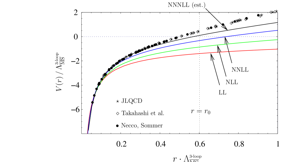
Figure 17: Comparison of $V_{\rm C+L}(r)$ in the $\mu_{f}$-independent scheme (solid lines) and the lattice data in quenched approximation [Takahashi et al. [48] ($\diamond$), Necco/Sommer [49] ($\bullet$), and JLQCD [50] ($\star$)]. Input parameters for $V_{\rm C+L}(r)$ are $\alpha_{S}(Q)=0.2$ and $n_{l}=0$; at NNNLL, Pineda’s estimate for $\bar{a}_{3}$ is used.

We see that $V_{\rm C+L}(r)$ up to different orders agree well with one another at small distances, whereas at large distances $V_{\rm C+L}(r)$ becomes steeper as we include higher-order terms via RG; cf. Tab. 2.

	LL	NLL	NNLL	NNNLL
${\cal C}^{\rm(R)}/\Bigl{(}\Lambda_{\overline{\rm MS}}^{\mbox{\scriptsize 3-loop}}\Bigr{)}^{2}$	0.1836	0.6950	1.261	1.758

Table 2: Coefficient of the linear potential [eq. (83)] in units of $\bigl{(}\Lambda_{\overline{\rm MS}}^{\mbox{\scriptsize 3-loop}}\bigr{)}^{2}$. Conventions are same as in Fig. 17.

This feature is in accordance with the qualitative understanding within perturbative QCD, in which the potential becomes steeper due to the running of the strong coupling constant, since $\alpha_{V}^{\rm PT}(q)$ increases more rapidly at IR as we include higher-order terms. The lattice data and $V_{\rm C+L}(r)$ also agree well at small distances, while they deviate at larger distances. More terms we include in $V_{\rm C+L}(r)$, up to larger distances the potential agrees with the lattice data. Theoretically, we expect $V_{\rm C+L}(r)$ to converge as we increase the order. The current status seems to be consistent with this expectation, since the lines in Fig. 17 apparently converge to the lattice data. One may adjust the input value $\alpha_{S}(Q)$ such that convergence becomes fast at some particular $r$; present choice $\alpha_{S}(Q)=0.2$ leads to a fast convergence at $r\Lambda_{\overline{\rm MS}}^{\mbox{\scriptsize 3-loop}}<0.1$. We may increase the value of input $\alpha_{S}(Q)$ such that convergence becomes fast at larger $r$. Then, $V_{\rm C+L}(r)$ up to different orders come closer to one another at $r\,\Lambda_{\overline{\rm MS}}^{\mbox{\scriptsize 3-loop}}>0.1$. [The relation between $V_{\rm C+L}(r)$ up to NNLL and the lattice data remains unchanged, since we use the 3-loop RG relation to fix the lattice scale, i.e. this relation is invariant under 3-loop RG evolution.]

Next we compare the renormalized singlet potential $V_{S}^{\rm(R)}(r;\mu_{f})$ for different values of the factorization scale $\mu_{f}$. In Fig. 18, we plot $V_{S}^{\rm(R)}(r;\mu_{f})$ up to NNLL for $\mu_{f}/\Lambda_{\overline{\rm MS}}^{\mbox{\scriptsize 3-loop}}=2$,3,4,5. Note that, up to NNLL, there is no distinction between the first scheme and the second scheme of Sec. 4.1.

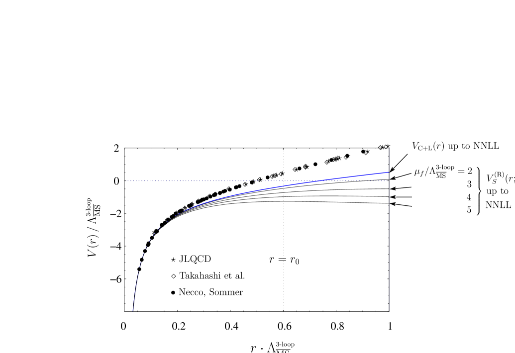
Figure 18: Comparison of lattice data and $V_{S}^{\rm(R)}(r;\mu_{f})$ up to NNLL for $\mu_{f}/\Lambda_{\overline{\rm MS}}^{\mbox{\scriptsize 3-loop}}=2$ to 5 (downwards). As a reference, we also plot $V_{\rm C+L}(r)$ up to NNLL. The lattice data and parameters for $V_{S}^{\rm(R)}(r;\mu_{f})$ and $V_{\rm C+L}(r)$ are same as in Fig. 17.

We see that $V_{\rm C+L}(r)$ is located closer to the lattice data than $V_{S}^{\rm(R)}(r;\mu_{f})$ for all $\mu_{f}$. As we vary $\mu_{f}$, the variation of $V_{S}^{\rm(R)}(r;\mu_{f})$ is larger at larger distances. As we lower $\mu_{f}$, $V_{S}^{\rm(R)}(r;\mu_{f})$ approaches $V_{\rm C+L}(r)$. These features are in agreement with the argument given in Sec. 4.3. Note that we cannot lower $\mu_{f}$ below the Landau singularity $q_{*}^{\mbox{\scriptsize 3-loop}}\approx 1.53\,\Lambda_{\overline{\rm MS}}^{\mbox{\scriptsize 3-loop}}$. $V_{S}^{\rm(R)}(r;\mu_{f})$ up to different orders behave similarly: As $\mu_{f}$ is lowered, $V_{S}^{\rm(R)}(r;\mu_{f})$ is raised at larger distances, approaching $V_{\rm C+L}(r)$ up to the corresponding order. For fixed $\mu_{f}$, $V_{S}^{\rm(R)}(r;\mu_{f})$ agrees with lattice data up to larger distances as we increase the order.

We turn to the measurement of $\delta E_{\rm US}(r)$. In computing $\delta E_{\rm US}(r)$, we use the lattice data from Table 2 of [49] for a non-perturbative computation of $V_{\rm QCD}(r)$, since this data set seems to be most accurate at short distances. In Fig. 19(a), we plot $\delta E_{\rm US}(r)$ in the C+L scheme [$V_{\rm QCD}(r)-V_{\rm C+L}(r)$] in units of $\Lambda_{\overline{\rm MS}}^{\mbox{\scriptsize 3-loop}}$. The errors of the data points, due to the errors of the lattice data for $V_{\rm QCD}(r)$, are comparable to or smaller than the sizes of the symbols used for the plot. Also shown in the same figure are fits to the data points of the form $A_{1}\,\rho+A_{2}\,\rho^{2}+A_{3}\,\rho^{3}$, where $\rho=r\,\Lambda_{\overline{\rm MS}}^{\mbox{\scriptsize 3-loop}}$. Only the data points in the range $r\,\Lambda_{\overline{\rm MS}}^{\mbox{\scriptsize 3-loop}}<0.5$ were used for the fits. We have added $r$-independent constants such that all the fits go through the origin. As we increase the order, $\delta E_{\rm US}(r)$ becomes smaller. We see that the cubic fit becomes a better approximation in a wider range in $r\,\Lambda_{\overline{\rm MS}}^{\mbox{\scriptsize 3-loop}}<1$ as we increase the order. [Here, we determine $\delta E_{\rm US}(r)$ in expansion in $r$, hence, we fit the data in the small $r$ region ($r\,\Lambda_{\overline{\rm MS}}^{\mbox{\scriptsize 3-loop}}<0.5$); it helps to enhance sensitivity to the coefficients of $r^{n}$ for small $n$. Since $\delta E_{\rm US}(r)\sim{\cal O}(\Lambda_{\rm QCD}^{4}r^{3})$ at sufficiently small $r$, i.e. $\delta E_{\rm US}(r)\to 0$ as $r\to 0$, it would make sense to perform a polynomial fit; however, in the next subsection, we reconsider this naive picture and give a more complete analysis.]

\psfrag{LL}{\footnotesize LL}\psfrag{NLL}{\hskip 5.69054pt\footnotesize NLL}\psfrag{NNLL}{\footnotesize NNLL}\psfrag{NNNLL}{\footnotesize NNNLL}\psfrag{Large-beta0}{\footnotesize large-$\beta_{0}$ appr.}\psfrag{r0}{ $r=r_{0}$}\psfrag{delEUS}{ $\delta E_{\rm US}(r)/\Lambda_{\overline{\rm MS}}^{\mbox{\scriptsize 3-loop}}$~{}~{} (C+L scheme)}\psfrag{r}{ $r\cdot\Lambda_{\overline{\rm MS}}^{\mbox{\scriptsize 3-loop}}$}\includegraphics[width=221.93158pt]{delEUS.eps}

\psfrag{NNLL, muf=3}{\footnotesize NNLL, $\mu_{f}=3\,\Lambda_{\overline{\rm MS}}^{\mbox{\tiny 3-loop}}$}\psfrag{NNLL, muf=5}{\footnotesize NNLL, $\mu_{f}=5\,\Lambda_{\overline{\rm MS}}^{\mbox{\tiny 3-loop}}$}\psfrag{NNNLL, muf=3}{\footnotesize NNNLL, $\mu_{f}=3\,\Lambda_{\overline{\rm MS}}^{\mbox{\tiny 3-loop}}$}\psfrag{NNNLL, muf=5}{\footnotesize NNNLL, $\mu_{f}=5\,\Lambda_{\overline{\rm MS}}^{\mbox{\tiny 3-loop}}$}\psfrag{r0}{ $r=r_{0}$}\psfrag{delEUS}{ $\delta E_{\rm US}(r)/\Lambda_{\overline{\rm MS}}^{\mbox{\scriptsize 3-loop}}$~{}~{}(factorization scheme)}\psfrag{r}{ $r\cdot\Lambda_{\overline{\rm MS}}^{\mbox{\scriptsize 3-loop}}$}\includegraphics[width=219.08612pt]{delEUS-VS.eps}

(a)                                                                            (b)

Figure 19: $\delta E_{\rm US}(r)/\Lambda_{\overline{\rm MS}}^{\mbox{\scriptsize 3-loop}}$ vs. $r\,\Lambda_{\overline{\rm MS}}^{\mbox{\scriptsize 3-loop}}$. The lattice data from Tab. 2 of [49] are used. Parameters for $V_{\rm C+L}(r)$ and $V_{S}^{\rm(R)}(r;\mu_{f})$ are same as in Fig. 17. Lines represent fits to the data points in the range $r\,\Lambda_{\overline{\rm MS}}^{\mbox{\scriptsize 3-loop}}<0.5$ by third-order polynomials, given explicitly in Tab. 3. (a) C+L scheme, up to LL, NLL, NNLL and NNNLL; C+L scheme in the large-$\beta_{0}$ approximation is also shown. (b) first scheme within the factorization scheme (subtraction of IR divergences by $\overline{\rm MS}$ scheme); for display purposes, $\delta E_{\rm US}(r)/\Lambda_{\overline{\rm MS}}^{\mbox{\scriptsize 3-loop}}$ at NNLL are shifted by +1 vertically.

We can learn more detailed features from the explicit polynomials obtained from the fits, shown in Tab. 3.

	C+L scheme	factorization scheme	factorization scheme
		($\mu_{f}=3\Lambda_{\overline{\rm MS}}^{\mbox{\tiny 3-loop}}$)	($\mu_{f}=5\Lambda_{\overline{\rm MS}}^{\mbox{\tiny 3-loop}}$)
LL	$6.7\,\rho-9.6\,\rho^{2}+8.7\,\rho^{3}$
NLL	$3.5\,\rho-3.6\,\rho^{2}+3.6\,\rho^{3}$
NNLL	$1.6\,\rho-0.3\,\rho^{2}+0.8\,\rho^{3}$	$1.6\,\rho+0.9\,\rho^{2}+0.8\,\rho^{3}$	$1.5\,\rho+3.5\,\rho^{2}-0.8\,\rho^{3}$
NNNLL, 1st scheme		$0.7\,\rho+1.8\,\rho^{2}+0.1\,\rho^{3}$	$0.6\,\rho+5.0\,\rho^{2}-1.8\,\rho^{3}$
NNNLL, 2nd scheme	$0.7\,\rho+0.8\,\rho^{2}-0.1\,\rho^{3}$	$0.7\,\rho+2.0\,\rho^{2}-0.0\,\rho^{3}$	$0.6\,\rho+5.1\,\rho^{2}-1.9\,\rho^{3}$
Large-$\beta_{0}$ appr.	$-2.7\,\rho+10.9\,\rho^{2}-9.1\,\rho^{3}$

Table 3: Fits of $\delta E_{\rm US}(r)/\Lambda_{\overline{\rm MS}}^{\mbox{\tiny 3-loop}}$ by cubic polynomials in the region $\rho<0.5$, where $\rho=r\Lambda_{\overline{\rm MS}}^{\mbox{\tiny 3-loop}}$. (See Fig. 19 for plots.) The lattice data [49] are used. Parameters for $V_{\rm C+L}(r)$ and $V_{S}^{\rm(R)}(r;\mu_{f})$ are same as in Fig. 17.

The coefficient of the linear potential decreases as we increase the orders, from LL to NNNLL. Up to NNNLL, the coefficient in units of $(\Lambda_{\overline{\rm MS}}^{\mbox{\tiny 3-loop}})^{2}$ is about 0.7. We may compare this value with the string tension (coefficient of linear potential) extracted from the large-distance behavior of the lattice data $\sigma\approx 3.8\,(\Lambda_{\overline{\rm MS}}^{\mbox{\tiny 3-loop}})^{2}$ [49]. Thus, the linear potential in $\delta E_{\rm US}(r)$ is quite small comparatively at our current best knowledge. We are interested in $\delta E_{\rm US}(r)$ in the infinite-order limit. Up to our current best knowledge, however, $\delta E_{\rm US}(r)$ in the C+L scheme has not stabilized yet, although we see a tendency that it approaches a quadratic form. We conclude that the present status is consistent with $\delta E_{\rm US}(r)$ in the infinite-order limit being order $\Lambda_{\rm QCD}^{3}r^{2}$ at $r\,\Lambda_{\overline{\rm MS}}^{\mbox{\scriptsize 3-loop}}\hbox{ \raise 3.0pt\hbox to0.0pt{$<$}\raise-3.0pt\hbox{$\sim$} }1$ (vanishing linear potential). From Figs. 17 and 19(a), it is not clear whether the limit would also be consistent with order $\Lambda_{\rm QCD}^{4}r^{3}$ or with zero. We will clarify this point quantitatively in the next subsection.

In Fig. 19(b) are plotted $\delta E_{\rm US}(r)$ in the first scheme (IR divergences of $\alpha_{V}^{\rm PT}(q)$ are subtracted in $\overline{\rm MS}$ scheme) within the factorization scheme [$V_{\rm QCD}(r)-V_{S}^{\rm(R)}(r;\mu_{f})$]. In this figure and in Tab. 3, we see that $\delta E_{\rm US}(r;\mu_{f})$ approximate the quadratic form ${\cal O}(\mu_{f}^{3}r^{2})$ expected from OPE. Approximation to the quadratic form is more evident than in the C+L scheme, since the coefficents of the quadratic terms are larger. Differences between the first and second scheme in the factorization scheme are tiny: If we plot, in the same figure, $\delta E_{\rm US}(r)$ in the second scheme (IR divergences of $\alpha_{V}^{\rm PT}(q)$ are regularized by double expansion in $\alpha_{S}$ and $\log\alpha_{S}$), they are hardly distinguishable from the lines of first scheme. This is also confirmed by the explicit forms of the polynomial fits in Tab. 3.

We may compare the fits of $\delta E_{\rm US}(r)$ in the factorization scheme and those in the C+L scheme in Tab. 3. The coefficients of linear terms are almost same in both schemes, up to NNLL and up to NNNLL, respectively. This confirms consistency with eq. (84). The difference of the coefficients of quadratic terms between both schemes is expected to be proportional to $\mu_{f}^{3}$ in the limit $\mu_{f}\gg\Lambda_{\rm QCD}$, according to eq. (84). This relation is roughly satisfied in Tab. 3 as well.

Next we compare $V_{\rm C+L}(r)$ in the large-$\beta_{0}$ approximation, analyzed in Sec. 3.2, with the lattice data. We take two different values of the input parameter: $\alpha_{S}(Q)=0.2$ and $\alpha_{S}(Q^{\prime})=0.5$, which correspond to $Q/\Lambda_{\overline{\rm MS}}^{\mbox{\scriptsize 1-loop}}=17.4$ and $Q^{\prime}/\Lambda_{\overline{\rm MS}}^{\mbox{\scriptsize 1-loop}}=3.1$, respectively. See Fig. 20.

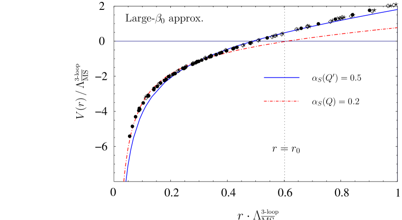
Figure 20: Comparison of $V_{\rm C+L}(r)$ in the large-$\beta_{0}$ approximation and lattice data. Inputs for $V_{\rm C+L}(r)$ are $\alpha_{S}(Q)=0.2$ and $\alpha_{S}(Q^{\prime})=0.5$. Other conventions are same as in Fig. 17.

Since the large-$\beta_{0}$ approximation incorporates only 1-loop running of $\alpha_{S}$, the prediction for $V_{\rm C+L}(r)$ is fairly scale dependent. Nevertheless, considering the crudeness of the approximation, agreement of the prediction with the lattice data is remarkably good. $V_{\rm C+L}(r)$ with $\alpha_{S}(Q)=0.2$ in Fig. 20 is much closer to the lattice data than $V_{\rm C+L}(r)$ at LL in Fig. 17. On the other hand, a more detailed examination reveals limitations of the large-$\beta_{0}$ approximation. In Fig. 19, we plot $\delta E_{\rm US}(r)$ computed from $V_{\rm C+L}(r)$ in the large-$\beta_{0}$ approximation with $\alpha_{S}(Q)=0.2$; a cubic fit using the data points at $r\Lambda_{\overline{\rm MS}}^{\mbox{\tiny 3-loop}}<0.5$ is shown in the same figure and in Tab. 3. Although the magnitude of $\delta E_{\rm US}(r)$ is small, $\delta E_{\rm US}(r)$ is oscillatory. The sizes of the coefficients of the polynomial fit are unnaturally large, and the fit does not reproduce $\delta E_{\rm US}(r)$ beyond $r\Lambda_{\overline{\rm MS}}^{\mbox{\tiny 3-loop}}=0.5$. Since there is no reason to believe that the large-$\beta_{0}$ approximation is very close to the infinite-order limit, we consider the different behaviors between $\delta E_{\rm US}(r)$ in this case and that of RG analysis (LL – NNNLL) to be an indication that the consistency checks performed in this subsection have sensitivity to the details.

5.2 Determinations of $r_{0}\Lambda_{\overline{\rm MS}}$ and $\delta E_{\rm US}(r)$ in C+L scheme

From the above analysis, we conclude that all the theoretical expectations derived from OPE are either positively confirmed or consistent with lattice data within the present level of uncertainties. In this subsection, with the aid of theoretical predictions of OPE, we estimate the infinite-order limit of $\delta E_{\rm US}(r)$ in the C+L scheme.

Up to this point, we used the central value (0.602) of the relation between $r_{0}$ and $\Lambda_{\overline{\rm MS}}^{\mbox{\scriptsize 3-loop}}$ in eq. (87). Now we examine how our determination of $\delta E_{\rm US}(r)$ will be affected if we vary this relation. To simplify the argument, for the moment let us suppose that the lattice data set (when expressed in units of $r_{0}$) has no errors and $V_{\rm C+L}(r)$ in the infinite-order limit is known. Let $V_{\rm latt}(r;x)$ represent the lattice data set converted to units of $\Lambda_{\overline{\rm MS}}^{\mbox{\scriptsize 3-loop}}$ using a given value of $x\equiv r_{0}\Lambda_{\overline{\rm MS}}^{\mbox{\scriptsize 3-loop}}$. Then, if $x$ equals its precise value $x_{\rm true}$, according to OPE, $\delta E_{\rm US}(r)=V_{\rm latt}(r;x_{\rm true})-V_{\rm C+L}(r)$ goes to zero as $r\to 0$ (ignoring an $r$-independent constant), hence, it would be approximated reasonably well by a polynomial of $r$. When $x$ differs from $x_{\rm true}$, we thus expect

$$V_{\rm diff}(r;x)\equiv V_{\rm latt}(r;x)-V_{\rm C+L}(r)$$

$$~{}~{}~{}~{}~{}~{}~{}~{}~{}~{}~{}~{}~{}\,=V_{\rm latt}(r;x_{\rm true})-V_{\rm C+L}(r)+V_{\rm latt}(r;x)-V_{\rm latt}(r;x_{\rm true})$$

$$~{}~{}~{}~{}~{}~{}~{}~{}~{}~{}~{}~{}~{}\,\approx P(r)+\Delta(r;x,x_{\rm true}),$$ (88)

where $P(r)$ is a polynomial of $r$, and

$$\Delta(r;x,x^{\prime})\equiv V_{\rm latt}(r;x)-V_{\rm latt}(r;x^{\prime}).$$ (89)

If we know $V_{\rm latt}(r;x)$ for some value of $x$, we can find $V_{\rm latt}(r;x)$ for other values of $x$ via

$$V_{\rm latt}(r;x^{\prime})=V_{\rm latt}\left(r\frac{x}{x^{\prime}};x\right)\,\frac{x}{x^{\prime}}.$$ (90)

On the other hand, we know that $V_{\rm latt}(r;x)$ tends to  ${\rm const.}\times(r\log|r\Lambda_{\overline{\rm MS}}|)^{-1}$ at short distances, while it tends to a linear potential at large distances. Then, one readily finds that $\Delta(r;x,x_{\rm true})$ has approximately a “Coulomb”+linear form at $r\,\Lambda_{\overline{\rm MS}}^{\mbox{\scriptsize 3-loop}}\hbox{ \raise 3.0pt\hbox to0.0pt{$<$}\raise-3.0pt\hbox{$\sim$} }1$ if $x\neq x_{\rm true}$.

In fact, by varying $x=r_{0}\Lambda_{\overline{\rm MS}}^{\mbox{\scriptsize 3-loop}}$ within the range given by eq. (87), we find a very good fit of $V_{\rm diff}(r;x)$:

$$V_{\rm diff}(r;x)\approx\Delta(r;x,0.596)+(0.8\,\rho+0.7\,\rho^{2})\,\Lambda_{\overline{\rm MS}}^{\mbox{\scriptsize 3-loop}}\biggr{|}_{\rho=r\Lambda_{\overline{\rm MS}}^{\mbox{\tiny 3-loop}}}.~{}~{}~{}~{}~{}\mbox{[NNNLL, $\bar{a}_{3}$(Pineda)]}$$

(91)

Inclusion of $\Delta(r;x,x^{\prime})$ into the fitting function stabilizes the fit considerably when $r_{0}\Lambda_{\overline{\rm MS}}^{\mbox{\tiny 3-loop}}$ is far from its optimal value (0.596): The coefficients of the linear and quadratic terms are much less affected even if we include cubic term in the fitting function or even if we use data points up to larger $r$ for the fit, whereas they are very unstable without $\Delta(r;x,x^{\prime})$ in the fitting function. A further examination shows that it is the inclusion of a Coulombic term (it does not matter very much whether log corrections are included or not) that stabilizes the fit when $r_{0}\Lambda_{\overline{\rm MS}}^{\mbox{\tiny 3-loop}}$ is far from its optimal value. In principle we should have included $\Delta(r;x,x^{\prime})$ in the fitting function in the previous subsection. A posteriori, it is because the central value of eq. (87) happened to be close to the optimal value in eq. (91) that polynomial fits were relatively stable (in particular as we increase the order) and all the features seemed quite consistent with the theoretical expectations.

We note that the error of the input $r_{0}\Lambda_{\overline{\rm MS}}^{\mbox{\scriptsize 3-loop}}$ in eq. (87) is sizable with regard to the accuracy of $V_{\rm C+L}(r)$ in our analysis. Indeed, in [26], the error of the input $r_{0}\Lambda_{\overline{\rm MS}}^{\mbox{\scriptsize 3-loop}}$ was the largest source of errors in the determination of $\delta E_{\rm US}(r)$. Conversely, this means that our analysis has a sensitivity to determine the relation between $r_{0}$ and $\Lambda_{\overline{\rm MS}}^{\mbox{\scriptsize 3-loop}}$ by itself (and possibly reduce the error of $\delta E_{\rm US}(r)$ at the same time). Hence, in our determination of $\delta E_{\rm US}(r)$, we will determine the value of $x=r_{0}\Lambda_{\overline{\rm MS}}^{\mbox{\scriptsize 3-loop}}$ simultaneously, by performing a fit to the data for $V_{\rm diff}(r;x)=V_{\rm latt}(r;x)-V_{\rm C+L}(r)$.

We approximate $\delta E_{\rm US}(r)$ by quadratic function $(A_{0}+A_{1}\,\rho+A_{2}\,\rho^{2})\Lambda_{\overline{\rm MS}}^{\mbox{\tiny 3-loop}}$ at $\rho=r\,\Lambda_{\overline{\rm MS}}^{\mbox{\scriptsize 3-loop}}\hbox{ \raise 3.0pt\hbox to0.0pt{$<$}\raise-3.0pt\hbox{$\sim$} }0.5$. As for errors, we take into account three types of sources: (i) errors of the lattice data, (ii) error of $\bar{a}_{3}$, and (iii) error due to higher-order corrections. Then we compute the probability density distribution for the parameters $(A_{0},A_{1},A_{2},x)$ in the following way. Define

$$\chi_{V}^{\,2}=\sum_{i=1}^{11}\left[\frac{V_{\rm latt}(r_{i};x)-\{V_{\rm C+L}(r_{i};s)+t\,\delta V_{\rm C+L}(r_{i})\}-(A_{0}+A_{1}\,\rho_{i}+A_{2}\,\rho_{i}^{2})\Lambda_{\overline{\rm MS}}^{\mbox{\tiny 3-loop}}}{\delta^{V}_{i}(x)}\right]^{2},\rule[-19.91692pt]{0.0pt}{17.07164pt}$$ (92)

$$P^{V}(A_{0},A_{1},A_{2},x)={\cal N}_{V}^{\,-1}\int ds\,dt\,\,e^{-\chi_{V}^{2}/2}\,P_{s}(s)\,P_{t}(t),$$ (93)

where $x=r_{0}\,\Lambda_{\overline{\rm MS}}^{\mbox{\scriptsize 3-loop}}$ and $\rho_{i}=r_{i}\,\Lambda_{\overline{\rm MS}}^{\mbox{\scriptsize 3-loop}}$. The normalization constant ${\cal N}_{V}$ is chosen such that the integral of $P^{V}(A_{0},A_{1},A_{2},x)$ over the entire range is unity. $s$ and $t$ parametrize errors of the theoretical prediction for $V_{\rm C+L}(r)$. Details are as follows.

1. We use the first 11 lattice data points given in Tab. 2 of [49]. $r_{i}=r_{i}(x)$ denotes the distance $r$ of the $i$-th lattice data point (given originally in units of $r_{0}$ and $r_{c}$) after conversion to units of $\Lambda_{\overline{\rm MS}}^{\mbox{\scriptsize 3-loop}}$, using $x=r_{0}\,\Lambda_{\overline{\rm MS}}^{\mbox{\scriptsize 3-loop}}$; $\delta^{V}_{i}(x)$ denotes the error of the $i$-th lattice data point (given originally in units of $r_{0}$) after conversion to units of $\Lambda_{\overline{\rm MS}}^{\mbox{\scriptsize 3-loop}}$. The first 11 data points correspond to $\rho_{i}<0.5$ when $x=0.602$.

2. $V_{\rm C+L}(r;s)$ denotes $V_{\rm C+L}(r)$ up to NNNLL evaluated with $\bar{a}_{3}=s\times\bar{a}_{3}({\rm Pineda})$. We scan $s$ between 0 and 2 with equal weight, i.e. $P_{s}(s)=1/2$ if $0\leq s\leq 2$ and $P_{s}(s)=0$ otherwise. The interval $0\leq s\leq 2$ covers within its range the estimates of $\bar{a}_{3}$ by Pineda [26], by Chishtie-Elias [13] and by large-$\beta_{0}$ approximation.

3. $t\,\delta V_{\rm C+L}(r)$ represents an estimate of the difference between $V_{\rm C+L}(r)$ up to NNNLL and $V_{\rm C+L}(r)$ in the infinte-order limit. $\delta V_{\rm C+L}(r)$ is estimated by the difference between $V_{\rm C+L}(r)$ up to NNLL and that up to NNNLL. We scan $t$ between $-1$ and 1 with equal weight, i.e. $P_{t}(t)=1/2$ if $|t|\leq 1$ and $P_{t}(t)=0$ otherwise.

Alternatively we may use the QCD force $F_{\rm QCD}(r)=dV_{\rm QCD}/dr$ in the determination of $\delta E_{\rm US}(r)$ and $x$. Since we are not interested in the $r$-independent part of the potential, we can extract information on the relevant parameters using the force as well. Similarly to before, we define

$$\chi_{F}^{\,2}=\sum_{i=1}^{10}\left[\frac{F_{\rm latt}(r_{i};x)-\{V_{\rm C+L}^{\prime}(r_{i};s)+t\,\delta V_{\rm C+L}^{\prime}(r_{i})\}-(A_{1}+2\,A_{2}\,\rho_{i})\Lambda_{\overline{\rm MS}}^{\mbox{\tiny 3-loop}}}{\delta^{F}_{i}(x)}\right]^{2},\rule[-19.91692pt]{0.0pt}{17.07164pt}$$ (94)

$$P^{F}(A_{1},A_{2},x)={\cal N}_{F}^{\,-1}\int ds\,dt\,\,e^{-\chi_{F}^{2}/2}\,P_{s}(s)\,P_{t}(t).$$ (95)

We use the first 10 points of the lattice data for $\{F_{\rm latt}(r_{i}),\,\delta^{F}_{i}(r_{i})\}$, corresponding to $\rho_{i}(0.602)<0.5$, given in the same table (Tab. 2) in [49]. Other details are same as in the case using the potential.

There is a considerable difference between the use of the potential and the force in the determination of $\delta E_{\rm US}(r)$ and $x$. The difference stems from different correlations of the errors ($\{\delta^{V}_{i}\}$, $\{\delta^{F}_{i}\}$) of the respective lattice data sets and from our treatment of these errors. It is known that there exists a high correlation among the errors of the lattice data at different $r_{i}$, for the QCD potential or for the force. It is also known that the error correlation of the force is smaller than that of the potential [51]. On the other hand, up to now, the covariance matrix of the errors for neither of these quantities is available. We therefore decided to use the lattice data with Gaussian errors, neglecting the correlations; see eqs. (92) and (94). This treatment should, in general, result in overestimates of errors in the determination of $(A_{1},A_{2},x)$.

Using the QCD Potential
\psfrag{A1}{$A_{1}$}\psfrag{A2}{$A_{2}$}\psfrag{68pcCL}{\footnotesize 68\%}\psfrag{95pcCL}{\footnotesize 95\%}\includegraphics[width=250.38434pt]{contour-plot-AB.eps}	\psfrag{68pc}{\footnotesize 68\%}\psfrag{95pc}{\footnotesize 95\%}\psfrag{r0}{ $r=r_{0}$}\psfrag{delEUS}{ $\delta E_{\rm US}(r)/\Lambda_{\overline{\rm MS}}^{\mbox{\scriptsize 3-loop}}$~{}~{}(C+L scheme)}\psfrag{r}{ $\rho=r\cdot\Lambda_{\overline{\rm MS}}^{\mbox{\scriptsize 3-loop}}$}\includegraphics[width=190.63338pt]{bounds-delEUS.eps}
(i)	(ii)

Figure 21: (i) Contour plot of the probability density distribution $P^{V}_{A_{1}A_{2}}(A_{1},A_{2})$, corresponding to 68% and 95% CL regions. Cross represents $(A_{1},A_{2})$ with the highest probability density, $(A_{1},A_{2})=(0.40,0.76)$. (ii) Bounds on $\delta E_{\rm US}(r)$ in the C+L scheme corresponding to the regions of (i). Quadratic fit with the highest probability density is also plotted (blue line).

Using the QCD Force
\psfrag{A1}{$A_{1}$}\psfrag{A2}{$A_{2}$}\psfrag{68pcCL}{\footnotesize 68\%}\psfrag{95pcCL}{\footnotesize 95\%}\includegraphics[width=250.38434pt]{contour-plot-AB-force.eps}	\psfrag{68pc}{\footnotesize 68\%}\psfrag{95pc}{\footnotesize 95\%}\psfrag{r0}{ $r=r_{0}$}\psfrag{delEUS}{ $\delta E_{\rm US}(r)/\Lambda_{\overline{\rm MS}}^{\mbox{\scriptsize 3-loop}}$~{}~{}(C+L scheme)}\psfrag{r}{ $\rho=r\cdot\Lambda_{\overline{\rm MS}}^{\mbox{\scriptsize 3-loop}}$}\includegraphics[width=190.63338pt]{bounds-delEUS-force.eps}
(i)	(ii)

Figure 22: (i) Contour plot of the probability density distribution $P^{F}_{A_{1}A_{2}}(A_{1},A_{2})$, corresponding to 68% and 95% CL regions. Cross represents $(A_{1},A_{2})$ with the highest probability density, $(A_{1},A_{2})=(1.03,0.60)$. (ii) Bounds on $\delta E_{\rm US}(r)$ in the C+L scheme corresponding to the regions of (i). Quadratic fit with the highest probability density is also plotted (blue line).

\psfrag{x}{\large$x=r_{0}\,\Lambda_{\overline{\rm MS}}^{\mbox{\scriptsize 3-loop}}$}\psfrag{pdf}{Probability density distribution}\psfrag{using potential}{\hskip 19.91692pt$P^{V}_{x}(x)$}\psfrag{using force}{$P^{F}_{x}(x)$}\includegraphics[width=284.52756pt]{PDF-r0Lambda-comb.eps}

Figure 23: Probability density distributions $P^{V,F}_{x}(x)$ vs. $x$.

Bounds on $\delta E_{\rm US}(r)$ can be obtained from the probability density distributions for $(A_{1},A_{2})$, defined by

$$P^{V}_{A_{1}A_{2}}(A_{1},A_{2})=\int dx\,dA_{0}\,\,P^{V}(A_{0},A_{1},A_{2},x),$$ (96)

$$P^{F}_{A_{1}A_{2}}(A_{1},A_{2})=\int dx\,\,P^{F}(A_{1},A_{2},x).$$ (97)

Figs. 22,22(i) show contour plots of these probability density distributions corresponding to the 68% and 95% confidence level (CL) regions. The corresponding bounds on $\delta E_{\rm US}(r)$ in the C+L scheme are given by [see Figs. 22,22(ii)]

Using the potential:

$$~{}~{}~{}~{}~{}~{}~{}~{}~{}~{}~{}~{}\left\{\begin{array}[]{ll}-0.7\,\rho+1.0\,\rho^{2}<\delta E_{\rm US}(r)/\Lambda_{\overline{\rm MS}}^{\mbox{\scriptsize 3-loop}}<2.1\,\rho+0.2\,\rho^{2}{}{}{}{}{}&(\mbox{68\% CL})\rule[-11.38109pt]{0.0pt}{17.07164pt}\\ -1.3\,\rho+1.1\,\rho^{2}<\delta E_{\rm US}(r)/\Lambda_{\overline{\rm MS}}^{\mbox{\scriptsize 3-loop}}<3.7\,\rho-0.8\,\rho^{2}{}{}{}{}{}&(\mbox{95\% CL})\end{array}\right.\rule[-28.45274pt]{0.0pt}{17.07164pt}$$ (100)

Using the force:

$$~{}~{}~{}~{}~{}~{}~{}~{}~{}~{}~{}~{}\left\{\begin{array}[]{ll}~{}~{}\,0.2\,\rho+0.7\,\rho^{2}<\delta E_{\rm US}(r)/\Lambda_{\overline{\rm MS}}^{\mbox{\scriptsize 3-loop}}<2.0\,\rho+0.4\,\rho^{2}{}{}{}{}{}&(\mbox{68\% CL})\rule[-11.38109pt]{0.0pt}{17.07164pt}\\ -0.2\,\rho+0.8\,\rho^{2}<\delta E_{\rm US}(r)/\Lambda_{\overline{\rm MS}}^{\mbox{\scriptsize 3-loop}}<2.6\,\rho+0.2\,\rho^{2}{}{}{}{}{}&(\mbox{95\% CL})\end{array}\right.$$ (103)

These bounds are mutually consistent, and the latter bounds are tighter. Since the origin $(A_{1},A_{2})=(0,0)$ lies outside the 95% CL regions in Figs. 22,22(i), we conclude that $\delta E_{\rm US}(r)$ being ${\cal O}(\Lambda_{\rm QCD}^{4}r^{3})$ or $\delta E_{\rm US}(r)=0$ is disfavored. We see that positive $A_{2}$ is favored, in agreement with the fits in Tab. 3.

The probability density distributions for $x=r_{0}\,\Lambda_{\overline{\rm MS}}^{\mbox{\scriptsize 3-loop}}$ are defined by

$$P^{V}_{x}(x)=\int dA_{0}\,dA_{1}\,dA_{2}\,\,P^{V}(A_{0},A_{1},A_{2},x),$$ (104)

$$P^{F}_{x}(x)=\int dA_{1}\,dA_{2}\,\,P^{F}(A_{1},A_{2},x).$$ (105)

They are shown in Fig. 23. Each distribution is close to Gaussian, so we simply quote the mean and the standard deviation for $x$:

$$\mbox{\it Using the potential:}~{}~{}~{}~{}~{}~{}~{}~{}~{}x=0.592\pm 0.062\,,~{}~{}~{}~{}~{}~{}~{}~{}~{}~{}~{}~{}~{}~{}$$ (106)

$$\mbox{\it Using the force:}~{}~{}~{}~{}~{}~{}~{}~{}~{}~{}~{}~{}~{}~{}x=0.574\pm 0.042\,.$$ (107)

Note that we did not use the relation (87) at all to obtain these results. Our results are mutually consistent, as well as in excellent agreement with eq. (87). The error in eq. (107) is of similar size to (slightly smaller than) that in eq. (87).

Some comments are in order.

As explained above, the sensitivity to $x=r_{0}\,\Lambda_{\overline{\rm MS}}^{\mbox{\scriptsize 3-loop}}$ originates from the mixing of a Coulombic term in $V_{\rm diff}(r;x)$ when $x$ is different from its true value. The only assumption we made in the determination of $x$ is that $\delta E_{\rm US}(r)$ can be approximated by a quadratic polynomial of $r$ at $r\,\Lambda_{\overline{\rm MS}}^{\mbox{\scriptsize 3-loop}}\hbox{ \raise 3.0pt\hbox to0.0pt{$<$}\raise-3.0pt\hbox{$\sim$} }0.5$. Since $\delta E_{\rm US}(r)$ goes to zero at sufficiently small $r$ according to OPE, a polynomial fit should be reasonable. Effects of higher powers of $r$ is expected to be suppressed at small $r$. In fact, we made a consistency check by including $A_{3}\rho^{3}$ term into the fits of $\delta E_{\rm US}(r)$ and/or by varying the number of data points used for the fits. As we include more data points, errors determined from $P^{V}_{x}(x)$ and $P^{F}_{x}(x)$ decrease, respectively, while the quality of the quadratic fits tends to get worse (quality is better with the cubic fits). In any case, the obtained bounds on $x$ are consistent with eqs. (106) and (107). We found that our present choice, quadratic fit with the first 11 (10) data points, is close to optimal in performing the fits.

When we scan $s$ and $t$ between the intervals $(0,2)$ and $(-1,1)$, respectively, the minimum values of $\chi_{V}^{2}$ and $\chi_{F}^{2}$ vary between (0.5, 0.6) and (0.1, 0.2), respectively. Since the number of degrees of freedom is $N_{\mbox{\scriptsize dof}}=11-4=10-3=7$, both $(\chi_{V}^{2})_{\rm min}/N_{\mbox{\scriptsize dof}}$ and $(\chi_{F}^{2})_{\rm min}/N_{\mbox{\scriptsize dof}}$ are below 10%. This is consistent with existence of high correlations among the lattice errors at different $r_{i}$, which we mentioned already. We note that our errors in eqs. (100),(103),(106),(107) may be overestimated for this reason.

The difference between the bounds obtained by using the potential and force can be attributed to the difference of the correlations of the lattice errors. Since the correlation is larger for the potential, the errors of the lattice data are effectively more enhanced (overestimated) in our treatment, hence the bounds are wider when we use the potential. The lattice errors are the dominant source of errors in the determination of $(A_{1},A_{2})$ and $x$, both when we use the potential and force. In this sense, the covariance matrices of the lattice data are highly demanded.

Since the errors for $V_{\rm C+L}(r)$ (parametrized by $s$ and $t$) are much larger than the errors of the lattice data, one may wonder why the latter can be dominant source of errors with regard to the former. [Note that in Fig. 19 the errors of the lattice data are smaller or comparable to the size of the symbols used for the plot; the variation of $V_{\rm C+L}(r;s)$ with $s$ is comparable in size to $\delta V_{\rm C+L}(r)$.] This can be understood as follows:
(1) Practically, the measurement of $x$ is sensitive only to the “Coulomb” part of $V_{\rm diff}(r;x)$, hence only the “Coulomb” part of the errors matters. Let us denote by $V^{(n)}_{\rm C+L}(r)$ the difference between $V_{\rm C+L}(r)$ up to NⁿLL and $V_{\rm C+L}(r)$ up to N^n-1LL. Then we perform fits of $V^{(n)}_{\rm C+L}(r)/\Lambda_{\overline{\rm MS}}^{\mbox{\scriptsize 3-loop}}$ in the form $c_{-1}\,\rho^{-1}+c_{1}\,\rho+c_{2}\,\rho^{2}$, using the 11 data points evaluated at $r=r_{i}$. The results for $n=1,2,3$ are shown in Tab. 4.

$V^{(1)}_{\rm C+L}(r)/\Lambda_{\overline{\rm MS}}^{\mbox{\scriptsize 3-loop}}$	$-0.0153\,\rho^{-1}+1.1\,\rho-0.5\,\rho^{2}$
$V^{(2)}_{\rm C+L}(r)/\Lambda_{\overline{\rm MS}}^{\mbox{\scriptsize 3-loop}}$	$-0.0087\,\rho^{-1}+0.8\,\rho-0.2\,\rho^{2}$
$V^{(3)}_{\rm C+L}(r;s=1)/\Lambda_{\overline{\rm MS}}^{\mbox{\scriptsize 3-loop}}$	$-0.0028\,\rho^{-1}+0.5\,\rho-0.05\,\rho^{2}$
$[V^{(3)}_{\rm C+L}(r;s=2)-V^{(3)}_{\rm C+L}(r;s=1)]/\Lambda_{\overline{\rm MS}}^{\mbox{\scriptsize 3-loop}}$	$-0.0038\,\rho^{-1}+0.6\,\rho-0.08\,\rho^{2}$
$[V^{(3)}_{\rm C+L}(r;s=0)-V^{(3)}_{\rm C+L}(r;s=1)]/\Lambda_{\overline{\rm MS}}^{\mbox{\scriptsize 3-loop}}$	$+0.0038\,\rho^{-1}-0.6\,\rho+0.08\,\rho^{2}$

Table 4: Fits of $V^{(n)}_{\rm C+L}(r_{i})/\Lambda_{\overline{\rm MS}}^{\mbox{\scriptsize 3-loop}}$ in the form $c_{-1}\,\rho^{-1}+c_{1}\,\rho+c_{2}\,\rho^{2}$, using the 11 data points evaluated at $r=r_{i}(0.602)$.

Magnitudes of all the coefficients $c_{k}^{(n)}$ decrease as the order increases, if we take $s=1$ as a reference for $V^{(3)}_{\rm C+L}(r)$. This is natural, since $V^{(n)}_{\rm C+L}(r)\to 0$ as $n\to\infty$, therefore all $c_{k}^{(n)}\to 0$. Thus, it is quite reasonable to estimate the “Coulomb” part of the errors of $V_{\rm C+L}(r)$ by the “Coulomb” part included in $t\,V^{(3)}_{\rm C+L}(r;s=1)$ or by that included in $V^{(3)}_{\rm C+L}(r;s)-V^{(3)}_{\rm C+L}(r;s=1)$. In fact, these error estimates are encoded in our analysis. Noting that we neglect the correlation of the errors of the lattice data, the errors of the lattice data are indeed larger than the “Coulomb” part of the errors of $V_{\rm C+L}(r)$. [Of course, the argument given here is only for demonstration to understand the errors better. When we derived our results eqs. (100),(103),(106),(107), neither did we do a fit of the form $c_{-1}\,\rho^{-1}+c_{1}\,\rho+c_{2}\,\rho^{2}$ nor extract a “Coulomb” part.]
(2) There is a similar mechanism in the determination of $(A_{1},A_{2})$. Since $\Delta(r;x,x^{\prime})$ has a “Coulomb”+linear form, if a small admixture of “Coulomb” part is allowed in $V_{\rm diff}(r)$ due to the errors of the lattice data, the linear term attached to the “Coulomb” part mixes in as well. Hence, if the lattice errors are larger, allowing a “Coulomb” part to mix in, the bounds on $(A_{1},A_{2})$ spread mainly in the $A_{1}$ direction. This explains the difference of Figs. 22(i) and 22(i). Again, it is the size of the “Coulomb” part of the errors that matters.

Our results can be compared with the determination of $\delta E_{\rm US}(r)$ by Pineda [26]. It is the only study that determined the non-perturbative contribution using OPE, preceding our current work. There are some important differences between Pineda’s analysis and ours.

• Pineda used $x=r_{0}\,\Lambda_{\overline{\rm MS}}^{\mbox{\scriptsize 3-loop}}$ as an input parameter, given by eq. (87). Its error turns out to be the dominant source of errors in the determination of $\delta E_{\rm US}(r)$ (defined in RS scheme [14, 26]). On the other hand, in our analysis, we determine $x$ from a fit to the data.

• We estimate the error of the singlet potential (in the C+L scheme) by varying $s$ and $t$ between $0\leq s\leq 2$ and $|t|\leq 1$. On the other hand, Pineda estimates the error of the singlet potential (in RS scheme) by varying $\bar{a}_{3}$ between the range corresponding to $1/2<s<3/2$, while there is no estimate corresponding to variation of $t$, i.e. $t$ is fixed to zero. Thus, our error estimate of the singlet potential is more conservative.

• Pineda does not incorporate errors of the lattice data at all. On the other hand, in our analysis, they are included neglecting the correlation. Since our analysis is sensitive to a “Coulomb” part, the lattice errors are the major source of errors.

• The singlet potential in RS scheme contains ${\cal O}(\Lambda_{\rm QCD}^{3}r^{2})$ renormalon. It means that the singlet potential has an intrinsic uncertainty of this order. This essentially prevents a determination of $\delta E_{\rm US}(r)$ with better than ${\cal O}(\Lambda_{\rm QCD}^{3}r^{2})$ accuracy, because $\delta E_{\rm US}(r)=V_{\rm QCD}(r)-V_{S}(r)$ cannot be defined with better accuracy. On the other hand, our potential is free from the ${\cal O}(\Lambda_{\rm QCD}^{3}r^{2})$ renormalon (and also from the rest of IR renormalons). So, at least conceptually, there is a difference in the achievable accuracies between the two analyses.

Due to these differences, comparisons between our bounds on $\delta E_{\rm US}(r)$ and those of Pineda are not straightforward. An explicit bound obtained by Pineda, assuming a form $\delta E_{\rm US}(r)={\rm const.}\times r^{2}$, reads

$$|\delta E_{\rm US}(r)|<2.8~{}\bigl{(}\Lambda_{\overline{\rm MS}}^{\mbox{\scriptsize 3-loop}}\bigr{)}^{3}\,r^{2}~{}~{}~{}(\mbox{RS scheme, Pineda \cite[cite]{[\@@bibref{}{Pineda:2002se}{}{}]}}).$$ (108)

One way of comparison may be to perform a fit by setting $A_{1}=0$ in our analysis. From the probability density distribution $P^{F}_{A_{1}A_{2}}(0,A_{2})$, we obtain

$$0.7~{}\bigl{(}\Lambda_{\overline{\rm MS}}^{\mbox{\scriptsize 3-loop}}\bigr{)}^{3}\,r^{2}<\delta E_{\rm US}(r)<0.9~{}\bigl{(}\Lambda_{\overline{\rm MS}}^{\mbox{\scriptsize 3-loop}}\bigr{)}^{3}\,r^{2}~{}~{}~{}~{}~{}\left(\begin{tabular}[]{c}C+L scheme, $A_{1}=0$\\ 68\% CL using force\end{tabular}\right).$$ (111)

5.3 Determination of $\delta E_{\rm US}(r)$ in factorization scheme

We can also determine the size of $\delta E_{\rm US}(r;\mu_{f})$ in the factorization scheme. In fact, in the second scheme (within the factorization scheme), the purely non-perturbative contribution is common to that in the C+L scheme. This is because the difference of $\delta E_{\rm US}(r)$ is merely the difference of the Wilson coefficients $V_{\rm C+L}(r)$ and $V_{S}^{\rm(R)}(r;\mu_{f})$; it is given by (minus) the right-hand-side of eq. (85), which is systematically computable by means of perturbative expansion and log resummation via RG. So, our task reduces to estimating the infinit-order limit of eq. (85).

	$[V_{\rm C+L}(r)-V_{S}^{\rm(R)}(r;\mu_{f})]/\Lambda_{\overline{\rm MS}}^{\mbox{\tiny 3-loop}}$
LL	$0.53\,\rho^{2}+0.00\,\rho^{3}+\cdots$
NLL	$0.85\,\rho^{2}+0.07\,\rho^{3}+\cdots$
NNLL	$1.04\,\rho^{2}+0.27\,\rho^{3}+\cdots$
NNNLL	$1.02\,\rho^{2}+0.58\,\rho^{3}+\cdots$

Table 5: Expansion of $[V_{\rm C+L}(r)-V_{S}^{\rm(R)}(r;\mu_{f})]/\Lambda_{\overline{\rm MS}}^{\mbox{\scriptsize 3-loop}}$ in $\rho=r\Lambda_{\overline{\rm MS}}^{\mbox{\tiny 3-loop}}$, computed using eq. (85). We neglect $\rho$-independent constants. $V_{S}^{\rm(R)}(r;\mu_{f})$ is computed in the second scheme and with $\mu_{f}=3\Lambda_{\overline{\rm MS}}^{\mbox{\tiny 3-loop}}$. Other parameters for $V_{\rm C+L}(r)$ and $V_{S}^{\rm(R)}(r;\mu_{f})$ are same as in Fig. 17.

Using eq. (85), we calculate Taylor expansions of $V_{\rm C+L}(r)-V_{S}^{\rm(R)}(r;\mu_{f})$ in $r$, which are listed in Tab. 5 for $\mu_{f}=3\,\Lambda_{\overline{\rm MS}}^{\mbox{\scriptsize 3-loop}}$. We estimate errors by the size of the NNNLL corrections and obtain

$$[V_{\rm C+L}(r)-V_{S}^{\rm(R)}(r;3\,\Lambda_{\overline{\rm MS}}^{\mbox{\scriptsize 3-loop}})]/\Lambda_{\overline{\rm MS}}^{\mbox{\scriptsize 3-loop}}\approx(1.02\pm 0.02)\,\rho^{2}+(0.58\pm 0.31)\,\rho^{3}.~{}~{}~{}~{}~{}~{}(\rho<0.5)$$ (112)

Thus, $\delta E_{\rm US}(r;3\,\Lambda_{\overline{\rm MS}}^{\mbox{\scriptsize 3-loop}})$ in the factorization scheme (second scheme) is given by the sum of eqs. (103) and (112). Given the above estimate, estimating $V_{\rm C+L}(r)-V_{S}^{\rm(R)}(r;\mu_{f})$ for other value of $\mu_{f}$ is straightforward, since the difference of the integrals [eq. (85)] can be evaluated by integrating over $q$ along the real axis and the integrand is free from singularities; convergence is fairly good in this region of $q$, so one may simply use the prediction up to NNNLL.

By the same token, we can estimate $\delta E_{\rm US}(r)$ in the first scheme within the factorization scheme. The difference between the first scheme and second scheme is perturbatively computable. In practice, up to NNNLL, we do not find a significant difference between the first scheme and the second scheme. We consider that we may apply the above estimate (112) also to the first scheme within the factorization scheme.

6 Summary and Conclusions

In this paper, we analyzed the static QCD potential in the distance region relevant to heavy quarkonium spectroscopy, $0.5~{}{\rm GeV}^{-1}(0.1~{}{\rm fm})\hbox{ \raise 3.0pt\hbox to0.0pt{$<$}\raise-3.0pt\hbox{$\sim$} }r\hbox{ \raise 3.0pt\hbox to0.0pt{$<$}\raise-3.0pt\hbox{$\sim$} }5~{}{\rm GeV}^{-1}(1~{}{\rm fm})$, using perturbative expansion and OPE as basic theoretical tools. The analysis consists of three major steps:
(I) Behavior of the QCD potential at large orders of perturbative expansion was analyzed. As for the higher-order terms, we used the estimates by large-$\beta_{0}$ approximation or by RG equation; as for the renormalization scale $\mu$, we varied it around the minimal-sensitivity scale [or, more precisely the scale defined by eq. (21)]. Then the perturbative expansion of the QCD potential, truncated at ${\cal O}(\alpha_{S}^{N})$, was separated into a scale-independent (prescription-independent) part and scale-dependent (prescription-dependent) part when $N\gg 1$:

$$V_{N}(r)=V_{C}(r)+{\cal B}(N,\xi)+{\cal C}\,r+{\cal D}(r,N,\xi)+(\mbox{terms that vanish as $N\to\infty$}).$$ (113)

Here, $\xi$ is a parameter for changing the scale ($\xi=1$ corresponds to an optimal choice of scale). $V_{C}(r)$ is a “Coulomb” potential, which includes logarithmic corrections at short-distances; ${\cal B}$ is an $r$-independent constant; ${\cal C}\,r$ is a linear potential; ${\cal D}(r)$ behaves as $r^{3\xi-1}\times(\mbox{log corr.})$ if $\xi<1$, whereas it is ${\cal O}(r^{2})$ and divergent as $N\to\infty$ if $\xi\geq 1$. $V_{C}(r)$ and ${\cal C}\,r$ correspond to a renormalon-free part of $V_{N}(r)$ and are finite and independent of $\xi$; thus the scale-independent part has a “Coulomb”+linear form. On the other hand, ${\cal B}$ and ${\cal D}(r)$ correspond, respectively, to the ${\cal O}(\Lambda_{\rm QCD})$ IR renormalon and beyond ${\cal O}(\Lambda_{\rm QCD})$ IR renormalons (starting from the ${\cal O}(\Lambda_{\rm QCD}^{3}r^{2})$ renormalon) contained in $V_{N}(r)$; they are dependent on $\xi$ and divergent as $N\to\infty$ if $\xi$ is sufficiently large. Detailed analytic behaviors of each component have been studied.
(II) In the framework of OPE of the QCD potential, (a) we gave explicit renormalization prescriptions for the Wilson coefficient (singlet potential) $V_{S}^{\rm(R)}(r;\mu_{f})$, which belong to the class of conventional factorization schemes with a hard cutoff; (b) the scale-independent part of (I) was generalized and promoted to a Wilson coefficient $V_{\rm C+L}(r)$, which is independent of the factorization scale $\mu_{f}$. Both $V_{S}^{\rm(R)}(r;\mu_{f})$ and $V_{\rm C+L}(r)$ are free from IR renormalons and IR divergences. Several properties of these Wilson coefficients and of the corresponding non-perturbative contributions have been derived (partly already in [24]):

• $V_{S}^{\rm(R)}(r;\mu_{f})$ and $V_{\rm C+L}(r)$ can be computed systematically using perturbative expansion and log resummation via RG, and (in principle) the predictions can be improved to arbitrary precision. Hence, the corresponding non-perturbative contributions $\delta E_{\rm US}(r)$ are unambiguously defined.

• With the usual hierarchy condition $\Lambda_{\rm QCD}\ll\mu_{f}\ll 1/r$, the difference between $V_{S}^{\rm(R)}(r;\mu_{f})$ and $V_{\rm C+L}(r)$ is ${\cal O}(\mu_{f}^{3}r^{2})$ and perturbatively computable. $V_{\rm C+L}(r)$ is closer to $V_{\rm QCD}(r)$ than $V_{S}^{\rm(R)}(r;\mu_{f})$.

• $\delta E_{\rm US}(r)$ in the factorization scheme is ${\cal O}(\mu_{f}^{4}r^{3})$ at very short-distances ($\Delta V(r)\gg\mu_{f}$), whereas it is ${\cal O}(\mu_{f}^{3}r^{2})$ in a semi-short-distance region ($\Delta V(r)\ll\mu_{f}\ll 1/r$).

• $\delta E_{\rm US}(r)$ in the C+L scheme ($\mu_{f}$-independent scheme) is ${\cal O}(\Lambda_{\rm QCD}^{4}r^{3})$ at very short-distances ($\Delta V(r)\gg\Lambda_{\rm QCD}$), whereas its behavior cannot be predicted model-independently in a semi-short-distance region ($\Delta V(r)\sim\Lambda_{\rm QCD}$).

We conjectured that the region of our interest corresponds to a semi-short-distance region where $\Delta V(r)\sim\Lambda_{\rm QCD}\,(\ll\mu_{f})$.
(III) We computed $V_{S}^{\rm(R)}(r;\mu_{f})$ and $V_{\rm C+L}(r)$ numerically for $n_{l}=0$ at our current best knowledge (NNNLL with certain estimates of $\bar{a}_{3}$) and compared them with the lattice computations of $V_{\rm QCD}(r)$ in the quenched approximation. We confirmed that the theoretical predictions of (II) are either correct or consistent within the present level of uncertainties. We find that a linear potential in $\delta E_{\rm US}(r)$ reduces with increasing order, consistently with vanishing in the infinite-order limit; at NNNLL, it is much smaller than the string tension as determined by lattice simulations. Then, we performed fits of $V_{\rm diff}(r;x)\equiv V_{\rm latt}(r;x)-V_{\rm C+L}(r)$ and determined simultaneously $\delta E_{\rm US}(r)$ and $x=r_{0}\Lambda_{\overline{\rm MS}}^{\mbox{\scriptsize 3-loop}}$ (relation between Sommer scale and $\Lambda_{\overline{\rm MS}}$). A sensitivity to $x$ originates from mixing of a Coulombic term into $V_{\rm diff}(r;x)$ when $x$ differs from its true value. Both the QCD potential and QCD force were used for the fits. The latter resulted in tighter bounds due to a smaller correlation of lattice errors. We obtained

$$r_{0}\Lambda_{\overline{\rm MS}}^{\mbox{\scriptsize 3-loop}}=0.574\pm 0.042\,,$$ (114)

in excellent agreement with the determination via Schrödinger functional method, eq. (87) [47]. We also obtained

$$0.2\,\rho+0.7\,\rho^{2}<\delta E_{\rm US}(r)/\Lambda_{\overline{\rm MS}}^{\mbox{\scriptsize 3-loop}}<2.0\,\rho+0.4\,\rho^{2},~{}~{}~{}~{}~{} (\mbox{C+L scheme})$$ (115)

where $\rho=r\Lambda_{\overline{\rm MS}}^{\mbox{\scriptsize 3-loop}}$. [See also bounds on the coefficients of quadratic polynomial in Figs. 22,22(i).] In the factorization scheme, we obtain, for instance,

$$0.2\,\rho+1.7\,\rho^{2}<\delta E_{\rm US}(r;\mu_{f})/\Lambda_{\overline{\rm MS}}^{\mbox{\scriptsize 3-loop}}<2.0\,\rho+1.4\,\rho^{2}\,.~{}~{}~{}\left(\begin{array}[]{cc}\mbox{factorization scheme}\\ \mu_{f}=3\Lambda_{\overline{\rm MS}}^{\mbox{\scriptsize 3-loop}}\end{array}\right)$$ (118)

Estimating $\delta E_{\rm US}(r;\mu_{f})$ for other $\mu_{f}$ is easy. In the factorization scheme, the obtained bounds are consistent with ${\cal O}(\mu_{f}^{3}r^{2})$, rather than ${\cal O}(\mu_{f}^{4}r^{3})$. In the C+L scheme, the obtained bound is consistent with ${\cal O}(\Lambda_{\rm QCD}^{3}r^{2})$ (vanishing linear potential) at 95% CL, but existence of a small linear term is more favored; furthermore, $\delta E_{\rm US}(r)\sim{\cal O}(\Lambda_{\rm QCD}^{4}r^{3})$ or $\delta E_{\rm US}(r)=0$ is disfavored. Consequently, we find that $\mu_{f}\gg\Delta V(r)$, in accord with our conjecture. Also $\Delta V(r)\sim\Lambda_{\rm QCD}$ is more likely than $\Delta V(r)\gg\Lambda_{\rm QCD}$.

The analysis (I) provides a reasoning within perturbative QCD, why we observed agreement between the recent perturbative computations of the QCD potential with phenomenological potentials or lattice results: in the large-order limit, $V_{N}(r)$ does approach a “Coulomb”+linear form. It is quite intriguing that we can separate the renormalon-free part and renormalon-dominant part in a natural way. Furthermore, in this analysis, the coefficient of the linear potential can be computed analytically up to NNLL.

In (II) we defined renormalization prescriptions for $V_{S}^{\rm(R)}(r;\mu_{f})$, in which all the known IR renormalons are subtracted. Moreover, introduction of a factorization-scale independent scheme for the Wilson coefficient, $V_{\rm C+L}(r)$, is new. $V_{\rm C+L}(r)$ has some appealing theoretical features: it has no intrinsic uncertainties, is systematically computable, and is closer to $V_{\rm QCD}(r)$ than $V_{S}^{\rm(R)}(r;\mu_{f})$. In any case, since the differences between the different schemes are perturbatively computable with good accuracy, the C+L scheme would serve as a useful reference.

In the numerical analysis (III), the only assumption we made in the fits is that we can approximate $\delta E_{\rm US}(r)$ by a quadratic polynomial of $r$ at $r\Lambda_{\overline{\rm MS}}^{\mbox{\scriptsize 3-loop}}<0.5$. This should be reasonable since $\delta E_{\rm US}(r)\to 0$ as $r\to 0$ according to OPE. (An $r$-independent constant is irrelevant in our analysis.) We checked validity of the assumption by including cubic term and by varying the number of data points used for the fits.

In Fig. 17 we have seen apparent convergence of $V_{\rm C+L}(r)$ towards the lattice data, up to our current best knowledge. However, a closer examination of $\delta E_{\rm US}(r)$ in the C+L scheme revealed that $\delta E_{\rm US}(r)=0$ is disfavored. In fact, we have improved both quantitatively and conceptually (in the sense that we removed all the renormalons from the singlet potential) the bounds on $\delta E_{\rm US}(r)$, as compared to the pioneering study by Pineda [26].

The OPE analysis of the QCD potential provided, as a byproduct, a new method for determining $x=r_{0}\Lambda_{\overline{\rm MS}}^{\mbox{\scriptsize 3-loop}}$. Our current result gives an error comparable in size to the error of the conventional result using the Schrödinger functional method [47]. The mechanism for the sensitivity is fairly clear, as well as sources of errors are understood well. The present status is that the errors of the lattice data contribute more significantly than the errors of $V_{\rm C+L}(r)$. Hence, information on the correlation of the lattice errors (in particular, the covariant matrix) is highly demanded in order to reduce the error.

Finally let us comment on the applicable range of perturbative expansion and OPE of $V_{\rm QCD}(r)$. We saw in Fig. 17 that the current best perturbative prediction of the Wilson coefficient $V_{\rm C+L}(r)$ follows the lattice data up to $r\hbox{ \raise 3.0pt\hbox to0.0pt{$<$}\raise-3.0pt\hbox{$\sim$} }r_{0}\approx 0.5$ fm. We consider that the distance, at which string breaking occurs, serves as a measure of the distance where the perturbative expansion breaks down (in the theory with $n_{l}>0$). It is around 1 fm according to the recent lattice simulation [52]. It is clear that the string breaking phenomenon is non-perturbative and that the present perturbative computation of the QCD potential lacks ingredients necessary for description of this phenomenon. In the context of heavy quarkonium phenomenology, string breaking corresponds to the decay $\Upsilon(4S)\to B\bar{B}$. Since empirically the root-mean-square radius of $\Upsilon(4S)$ is around 1 fm, it is consistent with the lattice results. We also know empirically that phenomenological potentials are approximated well by a Coulomb+linear form at $r\hbox{ \raise 3.0pt\hbox to0.0pt{$<$}\raise-3.0pt\hbox{$\sim$} }1$ fm. It means that, if we separate heavy quark and antiquark, we have a sensitivity to the linear potential at distances before string breaking takes place. Thus, we consider $r\hbox{ \raise 3.0pt\hbox to0.0pt{$<$}\raise-3.0pt\hbox{$\sim$} }1$ fm [corresponding to heavy quarkonium states below $\Upsilon(4S)$] to be the range in which perturbative expansion may make sense. (Certainly more terms of the perturbative expansion need to be included in order to have an accurate prediction of $V_{\rm C+L}(r)$ as $r$ approaches 1 fm.) Already in this range the QCD potential exhibits a linear behavior in addition to the “Coulomb” part. Our analysis indicates that the qualitative argument presented at the end of Sec. 2.4 may be valid in this very range. Ultimately, it depends on whether the linear term in $\delta E_{\rm US}(r)$ is truly vanishing or not.

Appendices

Appendix A Basic Formulas

In this Appendix we present detailed formulas useful for computing $\alpha_{V}^{\rm PT}(q)$ up to NNNLO as well as $V_{N}(r)$ for a finite but large $N$.

The perturbative expansion of the $V$-scheme coupling in momentum space $\alpha_{V}^{\rm PT}(q)$ is defined by eqs. (2)–(5). The polynomials in eq. (4) up to NNNLO are given by

$$P_{0}(\ell)=a_{0},$$ (119)

$$P_{1}(\ell)=a_{1}+2\,a_{0}\,\beta_{0}\,\ell,$$ (120)

$$P_{2}(\ell)=a_{2}+(4\,a_{1}\,\beta_{0}+2\,a_{0}\,\beta_{1})\,\ell+4\,a_{0}\,{\beta_{0}}^{2}\,\ell^{2},$$ (121)

$$P_{3}(\ell)=a_{3}+(6\,a_{2}\,\beta_{0}+4\,a_{1}\,\beta_{1}+2\,a_{0}\,\beta_{2})\,\ell+(12\,a_{1}\,{\beta_{0}}^{2}+10\,a_{0}\,\beta_{0}\,\beta_{1})\,\ell^{2}+8\,a_{0}\,{\beta_{0}}^{3}\,\ell^{3},$$ (122)

where

$$\ell=\log(\mu/q).$$ (123)

The coefficients of the beta function $\beta_{n}$, defined by eq. (6), are given explicitly by

$$\beta_{0}=11-\frac{2}{3}n_{l},$$ (124)

$$\beta_{1}=102-\frac{38}{3}n_{l},$$ (125)

$$\beta_{2}=\frac{2857}{2}-\frac{5033}{18}n_{l}+\frac{325}{54}n_{l}^{2}~{}~{}~{}~{}~{}\mbox{\cite[cite]{[\@@bibref{}{Tarasov:1980au,Larin:1993tp}{}{}]}},$$ (126)

$$\beta_{3}=\frac{149753}{6}+3564\,\zeta_{3}$$

$$~{}~{}~{}~{}~{}+\left(-\frac{1078361}{162}-\frac{6508\,\zeta_{3}}{27}\right)\,{n_{l}}+\left(\frac{50065}{162}+\frac{6472\,\zeta_{3}}{81}\right)\,{{n_{l}}}^{2}+\frac{1093\,{{n_{l}}}^{3}}{729}~{}~{}~{}~{}~{}\mbox{\cite[cite]{[\@@bibref{}{vanRitbergen:1997va}{}{}]}},$$ (127)

where $\zeta_{3}=\zeta(3)=1.2020...$ denotes the Riemann zeta function $\zeta(z)=\sum_{n=1}^{\infty}{1}/{n^{z}}$ evaluated at $z=3$.

Presently, $a_{n}$ are known up to $n=2$.

$$a_{0}=1,$$ (128)

$$a_{1}=\frac{31}{3}-\frac{10}{9}n_{l}~{}~{}~{}~{}~{}\mbox{\cite[cite]{[\@@bibref{}{Appelquist:es,Fischler:1977yf}{}{}]}},~{}~{}~{}~{}~{}$$ (129)

$$a_{2}={\frac{4343}{18}}+36\,{{\pi}^{2}}+66\,{\zeta_{3}}-{\frac{9\,{{\pi}^{4}}}{4}}-\left({\frac{1229}{27}}+{\frac{52\,{\zeta_{3}}}{3}}\right)\,{n_{l}}+{\frac{100}{81}}\,{n_{l}^{2}}~{}~{}~{}~{}~{}\mbox{\cite[cite]{[\@@bibref{}{Peter:1996ig,Schroder:1998vy}{}{}]}}.$$ (130)

It is known that $a_{3}$ is IR divergent; the coefficient of the divergence and associated logarithm have been computed [10, 11]:

$$a_{3}={72\pi^{2}}\left[\,\frac{1}{\epsilon}+4\left\{2\ell+\log(4\pi)-\gamma_{E}\right\}\right]+\bar{a}_{3},$$ (131)

where the IR divergence is regularized by dimensional regularization ($D=4-2\epsilon$). $\bar{a}_{3}$ is just a constant independent of $\epsilon$, $\mu$, $r$. So far, only some estimates of its size are known: e.g. $\bar{a}_{3}(\mbox{large-}\beta_{0})=(\frac{5}{3}\beta_{0})^{3}\approx 6162$, $\bar{a}_{3}(\mbox{Pineda})\approx 18688$ [14, 26], $\bar{a}_{3}(\mbox{Chishtie-Elias})\approx 20032$ [13] for $n_{l}=0$.

Physical logarithm associated with the IR divergence can be extracted as follows [10, 24]. Instead of defining the ultrasoft contribution $\delta E_{\rm US}(r)$ in eq. (17) as a non-perturbative quantity, it can be computed in a double expansion in $\alpha_{S}$ and $\log\alpha_{S}$ within pNRQCD:

$$\Bigl{[}\delta E_{\rm US}(r)\Bigr{]}\!\!_{\mbox{\hbox{ \raise-3.0pt\hbox to0.0pt{\scriptsize double}\raise-11.0pt\hbox{\scriptsize exp.} } }}=\frac{C_{F}C_{A}^{3}\alpha_{S}(\mu)^{4}}{24\,\pi\,r}$$

$$~{}~{}~{}~{}~{}~{}~{}~{}~{}~{}~{}~{}~{}~{}~{}~{}~{}~{}~{}~{}~{}~{}~{}~{}~{}\times\left[\,\frac{1}{\epsilon}+8\log(\mu\,r)-2\log\Bigl{(}{C_{A}\alpha_{S}(\mu)}\Bigr{)}+\frac{5}{3}+2\gamma_{E}+4\log(4\pi)\right]+{\cal O}(\alpha_{S}^{5}),$$

(132)

where $\gamma_{E}=0.5772...$ denotes the Euler constant. Upon Fourier transform, $1/\epsilon$ and $\log\mu$ terms of eqs. (131) and (132) cancel each other. The remaining $\log(C_{A}\alpha_{S})$ is the physical logarithm. The argument of the logarithm in eq. (132), $C_{A}\alpha_{S}=2\,r\,\Delta V(r)$, represents the ratio of the IR regulator $2\Delta V(r)$ and $1/r$; cf. Sec. 2.4. If we perform OPE in conventional factorization schemes, we introduce the factorization scale $\mu_{f}$, and the IR regulator $2\Delta V(r)$ will be replaced by $\mu_{f}$. Thus, one finds the ultrasoft logarithm

$$V_{S}^{(\rm R)}(r;\mu_{f})\Bigr{|}_{\mbox{\scriptsize US-log}}=-\frac{C_{F}C_{A}^{3}\alpha_{S}(\mu)^{4}}{24\,\pi\,r}\times 2\log(\mu_{f}r).$$ (133)

It is easy to verify that the $\alpha_{S}(\mu)^{4}\,\log(\mu_{f}/q)$ term of eq. (7) generates eq. (133) after Fourier transform. (Oppositely, using RG equation with respect to evolution of $\mu_{f}$ within pNRQCD, one can resum US logs as given in eq. (7) [12].)

One may verify explicitly that $\alpha_{V}^{\rm PT}(q)$ up to NNNLO, defined via eqs. (119)–(131), and $\bigl{[}\delta E_{\rm US}(r)\bigr{]}_{\rm d.e.}$ in eq. (132) are separately consistent with RG equations with respect to evolution of $\mu$:

$$\left[\mu^{2}\frac{\partial}{\partial\mu^{2}}+\beta(\alpha_{S}(\mu))\frac{\partial}{\partial\alpha_{S}(\mu)}\right]X=0~{}~{}~{}~{}~{}~{}~{}~{};~{}~{}~{}~{}~{}~{}~{}~{}~{}X=\alpha_{V}^{\rm PT}(q)~{}~{}\mbox{or}~{}~{}\Bigl{[}\delta E_{\rm US}(r)\Bigr{]}\!\!_{\mbox{\hbox{ \raise-3.0pt\hbox to0.0pt{\scriptsize double}\raise-11.0pt\hbox{\scriptsize exp.} } }}$$ (134)

This should be so, as long as $V_{\rm QCD}(r)$ and $\alpha_{V}^{\rm PT}(q)$ are defined from the Wilson loop via eqs. (2)–(4), since the Wilson loop is independent of $\mu$. To verify eq. (134), one should note that the beta function in general dimension (in $\overline{\rm MS}$ scheme) has a form

$$\left[\beta(\alpha_{S})\right]_{\epsilon\neq 0}=-\epsilon\,\alpha_{S}+\left[\beta(\alpha_{S})\right]_{\epsilon=0}.$$ (135)

In the rest of this Appendix, we present formulas useful for computing $V_{N}(r)$ for a large (but finite) $N$. The expansion of $\alpha_{S}(q)^{n}$ in terms of $\alpha_{S}(\mu)$ can be obtained by iterative operation of a derivative operator as

$$\alpha_{S}(q)^{n}=\exp\left[-2\ell\,\beta(x)\frac{\partial}{\partial x}\right]\,x^{n}\Biggr{|}_{x\to\alpha_{S}(\mu)}$$

$$~{}~{}~{}~{}~{}~{}~{}~{}~{}=\sum_{k=0}^{\infty}\frac{(-2\ell)^{k}}{k!}\,\left[\beta(x)\frac{\partial}{\partial x}\right]^{k}\,x^{n}\Biggr{|}_{x\to\alpha_{S}(\mu)},$$ (136)

where $\beta(\alpha_{S})$ is defined in eq. (6) [and eq. (135) if necessary].

The $V$-scheme coupling in position space, $\bar{\alpha}_{V}(1/r)$, is defined by $V_{\rm QCD}(r)=-C_{F}\,\bar{\alpha}_{V}(1/r)/r$. The series expansion of $\bar{\alpha}_{V}(1/r)$ in terms of the $\overline{\rm MS}$ coupling renormalized at $\mu=\exp(-\gamma_{E})/r$ is obtained as follows [57]. Using the coefficients $g_{m}$ defined by

$$\sum_{m=0}^{\infty}g_{m}\,u^{m}=\exp\left[\sum_{k=2}^{\infty}\frac{\zeta(k)\,u^{k}}{k}\,\left\{2^{k}-1-(-1)^{k}\right\}\right],$$ (137)

we may write

$$\bar{\alpha}_{V}(1/r)=\sum_{m=0}^{\infty}g_{m}\left[-\beta(x)\frac{\partial}{\partial x}\right]^{m}\sum_{n=0}^{\infty}\frac{a_{n}}{(4\pi)^{n}}\,x^{n+1}\Biggr{|}_{x\to\alpha_{S}(\exp(-\gamma_{E})/r)}.$$ (138)

To obtain the expansion of $\bar{\alpha}_{V}(1/r)$ in terms of $\alpha_{S}(\mu)$, we first compute eq. (138), then substitute the expansions of $\alpha_{S}(\exp(-\gamma_{E})/r)^{n}$ in terms of $\alpha_{S}(\mu)$ computed using eq. (136). By truncating the series at an appropriate order in $\alpha_{S}(\mu)$, the result reduces to a polynomial of $\log(\mu\,r)$.

Appendix B Integral Representation of $[\alpha_{S}(q)]_{\infty}$ at NLL

$[\alpha_{S}(q)]_{\infty}$ for the 2-loop running coupling constant can be expressed in a one-parameter integral form. After integrating the RG equation, $\alpha_{S}(q)$ is given implicitly by the relation

$$\log\left({q}/{\Lambda_{\overline{\rm MS}}^{\mbox{\scriptsize 2-loop}}}\right)=-\frac{2\pi}{\beta_{0}\alpha_{S}}+\frac{\delta}{2}\,\log\left(\frac{4\pi}{\beta_{0}\alpha_{S}}+\delta\right).$$ (139)

Hence, using Cauchy’s theorem, one may write

$$\alpha_{S}(q) = \frac{i}{\beta_{0}}\int_{C_{s}}ds\,(-s)^{-1}\,\left[\log\left({q}/{\Lambda_{\overline{\rm MS}}^{\mbox{\scriptsize 2-loop}}}\right)+\frac{\delta}{2}\,\log\left({-2es}\right)+s\right]^{-1}\rule[-22.76219pt]{0.0pt}{17.07164pt}$$

$$= \frac{i}{\beta_{0}}\int_{C_{s}}ds\,(-s)^{-1}\,\int_{0}^{\infty}dx\,\exp\left[-x\left\{\log\left({q}/{\Lambda_{\overline{\rm MS}}^{\mbox{\scriptsize 2-loop}}}\right)+\frac{\delta}{2}\,\log\left({-2es}\right)+s\right\}\right]\rule[-22.76219pt]{0.0pt}{17.07164pt}$$

$$= \frac{2\pi}{\beta_{0}}\int_{0}^{\infty}dx\,\left({q}/{\Lambda_{\overline{\rm MS}}^{\mbox{\scriptsize 2-loop}}}\right)^{-x}\left(\frac{x}{2e}\right)^{x\,\delta/2}\frac{1}{\Gamma(1+x\,\delta/2)}\,.$$ (141)

The integral contour $C_{s}$ is shown in Fig. 24. In the last equality, we rescaled $s\to s/x$ and used the formula $1/\Gamma(z)=i(2\pi)^{-1}\int_{C_{s}}ds\,(-s)^{-z}\,e^{-s}$.

\psfrag{Cs}{$C_{s}$}\psfrag{s}{$s$}\psfrag{0}{\raise 0.0pt\hbox{\footnotesize 0}}\includegraphics[width=142.26378pt]{pathCs.eps}

Figure 24: Integral contour $C_{s}$.

The truncated series expansion of $\alpha_{S}(q)$ in $\alpha_{\mu}\equiv\alpha_{S}(\mu)$ can be obtained as follows. One rewrites $\Lambda_{\overline{\rm MS}}^{\mbox{\scriptsize 2-loop}}$ in terms of $\alpha_{\mu}$ in eq. (B). After changing variables as $s=(\frac{4\pi}{\beta_{0}\alpha_{\mu}}+\delta)u$, we have

$$\alpha_{S}(q)=\frac{i\,\alpha_{\mu}}{2\pi}\int_{C_{u}}du\,(-u)^{-1}\,\left[1+\frac{u}{\alpha_{\mu}\delta+{4\pi}/{\beta_{0}}}+\frac{\beta_{0}\alpha_{\mu}}{2\pi}\left\{\log\Bigl{(}\frac{q}{\mu}\Bigr{)}+\frac{\delta}{2}\,\log(-eu)\right\}\right]^{-1}.$$ (142)

Expanding the integrand in $\alpha_{\mu}$ and integrating at each order of the expansion, one obtains the series expansion of $\alpha_{S}(q)$ in $\alpha_{\mu}$. It is then straightforward to truncate at order ${\alpha_{\mu}}^{N}$. Sending $N\to\infty$, we obtain

$$\lim_{N\to\infty}\left[\alpha_{\mu}\left[1+\frac{u}{\alpha_{\mu}\delta+{4\pi}/{\beta_{0}}}+\frac{\beta_{0}\alpha_{\mu}}{2\pi}\left\{\log\Bigl{(}\frac{q}{\mu}\Bigr{)}+\frac{\delta}{2}\,\log(-eu)\right\}\right]^{-1}\right]_{N}$$

$$~{}~{}~{}~{}~{}~{}~{}~{}~{}~{}~{}~{}=\left[\log\left({q}/{\Lambda_{\overline{\rm MS}}^{\mbox{\scriptsize 2-loop}}}\right)+\frac{\delta}{2}\,\log\left({-2es}\right)+s\right]^{-1}$$

$$~{}~{}~{}~{}~{}~{}~{}~{}~{}~{}~{}~{}~{}~{}~{}~{}~{}\times\left(1-\exp\left[-3\xi\left\{\log\left({q}/{\Lambda_{\overline{\rm MS}}^{\mbox{\scriptsize 2-loop}}}\right)+\frac{\delta}{2}\,\log\left({-2es}\right)+s\right\}\right]\right),$$ (143)

where we re-expressed the truncated series in terms of $s$ and $\Lambda_{\overline{\rm MS}}^{\mbox{\scriptsize 2-loop}}$. Similarly to eq. (141), we find

$$[\alpha_{S}(q)]_{\infty}=\frac{2\pi}{\beta_{0}}\int^{3\xi}_{0}dx\,\left({q}/{\Lambda_{\overline{\rm MS}}^{\mbox{\scriptsize 2-loop}}}\right)^{-x}\left(\frac{x}{2e}\right)^{x\,\delta/2}\frac{1}{\Gamma(1+x\,\delta/2)}.$$ (144)

Thus, the one-parameter integral forms given in eq. (56) are obtained.

Appendix C Analytic Formula of the Linear Potential in Case (c)

We present the analytic formula for the coefficient of the linear potential, defined by eq. (43), in case (c). The integral eq. (43) can be reduced to a one-parameter integral form by change of variables, e.g. from $q$ to $z=1/\alpha_{S}$. Then one readily sees that the integral can be expressed in terms of the confluent hypergeometric function except for the coefficient of $a_{2}$, while the coefficient of $a_{2}$ can be expressed in terms of generalized confluent hypergeometic functions.

For convenience, we first define some auxiliary parameters. The two solutions to the quadratic equation

$$\left.\frac{4\pi\,\beta(\alpha_{S})}{\alpha_{S}^{2}}\right|_{\rm case\,(c)}=-\sum_{n=0}^{2}\beta_{n}\,\Bigl{(}\frac{\alpha_{S}}{4\pi}\Bigr{)}^{n}=0$$ (145)

[cf. eq. (6)] are denoted as $\alpha_{S}=1/\omega$ and $1/\omega^{*}$. Then we define

$$p=\frac{2\pi}{\beta_{0}}\,\frac{\omega^{2}}{\omega-\omega^{*}}.$$ (146)

We also write $b_{0}=\beta_{0}/(4\pi)$.

The coefficient of the linear potential in case (c) is given by

$${\cal C}^{\rm(c)}=\frac{2\pi C_{F}}{\beta_{0}}\,\left(\Lambda^{\rm 3-loop}_{\overline{\rm MS}}\right)^{2}\,\left[a_{0}\,{\cal R}_{0}+\frac{a_{1}}{4\pi}\,{\cal R}_{1}+\frac{a_{2}}{(4\pi)^{2}}\,{\cal R}_{2}\right],$$ (147)

where

$${\cal R}_{0}=2\,{\rm Re}\left[\,F(p+{\textstyle\frac{1}{2}},p^{*})+\omega\,F(p,p^{*})\,\right],$$ (148)

$${\cal R}_{1}=2\,{\rm Re}\left[\,F(p,p^{*})\,\right],$$ (149)

$${\cal R}_{2}=2\,{\rm Re}\left[\,G\,\right]-{b_{0}}^{\delta}\,(-\omega)^{2p-1}\,(-\omega^{*})^{2p^{*}-1}.$$ (150)

The function $F$ is defined by

$$F(x,y) = {b_{0}}^{x+y+\delta}\,\frac{(\omega-\omega^{*})^{x+y-1}\,e^{-i\pi(x-y)-\delta/2}}{\Gamma(1-2x)}\,W_{y-x,\,x+y-1/2}\Bigl{(}{\textstyle\frac{\omega^{*}-\omega}{b_{0}}}\Bigr{)},$$ (151)

in terms of the Whittaker function, which is related to the confluent hypergeometric function ${}_{1}F_{1}$ as

$$W_{\kappa,\mu}(z) = \frac{\Gamma(-2\mu)}{\Gamma(\frac{1}{2}-\mu-\kappa)}\,z^{\mu+1/2}\,e^{-z/2}\,_{1}F_{1}(\mu-\kappa+{\textstyle\frac{1}{2}},2\mu+1;z)$$ (152)

$$+\frac{\Gamma(2\mu)}{\Gamma(\frac{1}{2}+\mu-\kappa)}\,z^{-\mu+1/2}\,e^{-z/2}\,_{1}F_{1}(-\mu-\kappa+{\textstyle\frac{1}{2}},-2\mu+1;z).$$

On the other hand, $G$ is defined by

$$G = {b_{0}}^{\delta}\,e^{(\omega/b_{0})+i\pi(2p^{*}-1)}\,$$ (153)

$$\times\biggl{\{}\,\frac{(\omega^{*}-\omega)^{-2-\delta}}{(1-2p)\,B(1-2p,1-2p^{*})}\,\Gamma_{1}\Bigl{(}1,2p-1,2+\delta;{\textstyle\frac{\omega}{\omega^{*}-\omega},\frac{\omega-\omega^{*}}{b_{0}}}\Bigr{)}$$

$$~{}~{}~{}-\frac{{b_{0}}^{-2-\delta}}{\pi}\,\sin(2\pi p)\,\Gamma(-2-\delta)\,\Xi_{2}\Bigl{(}1,1-2p^{*},3+\delta;{\textstyle-\frac{\omega}{b_{0}},\frac{\omega^{*}-\omega}{b_{0}}}\Bigr{)}\biggr{\}}.$$

$\Gamma_{1}$ and $\Xi_{2}$ represent Appell confluent hypergeometric functions [58] defined by the double series

$$\Gamma_{1}(\alpha,\beta,\beta^{\prime};x,y)=\sum_{m,n=0}^{\infty}\frac{(\alpha)_{m}(\beta)_{n-m}(\beta^{\prime})_{m-n}}{m!\,n!}\,x^{m}y^{n},$$ (154)

$$\Xi_{2}(\alpha,\beta,\gamma;x,y)=\sum_{m,n=0}^{\infty}\frac{(\alpha)_{m}(\beta)_{n}}{(\gamma)_{m+n}\,m!\,n!}\,x^{m}y^{n},$$ (155)

where $(a)_{n}\equiv\Gamma(a+n)/\Gamma(a)$ is the Pochhammer symbol.

Appendix D Numerical Evaluation of $V_{S}^{\rm(R)}(r;\mu_{f})$ and $V_{\rm C+L}(r)$

In this Appendix, we present a method for accurate numerical evaluations of $V_{S}^{\rm(R)}(r;\mu_{f})$ and $V_{\rm C+L}(r)$. The former is defined in Sec. 4.1 to be

$$V_{S}^{({\rm R})}\!(r;\mu_{f}\!)=-\frac{2C_{F}}{\pi}\!\!\int_{\mu_{f}}^{\infty}\!\!\!\!dq\,\frac{\sin(qr)}{qr}\,\alpha_{V_{S}}^{({\rm R})}(q;\mu_{f})$$ (156)

with

$$\alpha_{V_{S}}^{({\rm R})}(q;\mu_{f}) = \alpha_{V}^{\rm PT}\!(q)+\delta\alpha_{V}\!(q;\mu_{f})$$ (157)

$$= \alpha_{S}(q)\,\sum_{n=0}^{N}a^{V_{s}}_{n}\,\biggl{(}\frac{\alpha_{S}(q)}{4\pi}\biggr{)}^{n}.$$ (158)

$N=0,1,2$, and 3 correspond to $V_{S}^{\rm(R)}(r;\mu_{f})$ up to LL, NLL, NNLL and NNNLL, respectively. (We do not resum US logs but include only up to NNNLO.) $a^{V_{s}}_{n}=P_{n}(0)=a_{n}$ for $n\leq 2$, whose explicit forms are given in eqs. (128)–(130); $a^{V_{s}}_{3}=\bar{a}_{3}+144\pi^{2}\log(\mu_{f}/q)$ in the first scheme [corresponding to eq. (78)], while $a^{V_{s}}_{3}=\bar{a}_{3}-120\pi^{2}+144\pi^{2}\left\{\gamma_{E}+\log[3\alpha_{S}(q)]\right\}$ in the second scheme [corresponding to eq. (79)].

We deform the integral path of eq. (156) into upper half plane:

$$V_{S}^{({\rm R})}\!(r;\mu_{f}\!)=-\frac{2C_{F}}{\pi}\,{\rm Im}\int_{0}^{\infty}\!\!\!\!dk\,\left[i\,\frac{\exp(iqr)}{qr}\,\alpha_{V_{S}}^{({\rm R})}(q;\mu_{f})\right]_{q=\mu_{f}+i\,k}.$$ (159)

In order to evaluate the integral numerically, we first solve the RG equation (6) with a given input value (e.g. $\alpha_{S}(Q)=0.2$) and find the value of $Q/\Lambda_{\overline{\rm MS}}$ and the value of $\alpha_{S}(\mu_{f})$ for a given $\mu_{f}/\Lambda_{\overline{\rm MS}}$. Then we solve the RG equation (6) along the integral path $q=\mu_{f}+i\,k$  ($0<k<\infty$) in the complex plane, with $\alpha_{S}(\mu_{f})$ as the initial value. In solving the RG equation, we take the sum for $n\leq 0,1,2$ and 3 on the right-hand-side of eq. (6), respectively, corresponding to $V_{S}^{\rm(R)}(r;\mu_{f})$ up to LL, NLL, NNLL and NNNLL.

The singlet potential in the $\mu_{f}$-independent scheme $V_{\rm C+L}(r)$ is defined in Secs. 4.1 and 4.2. It is easier to evaluate the difference $V_{S}^{\rm(R)}(r;\mu_{f})-V_{\rm C+L}(r)$ accurately, using eq. (85), than to directly evaluate $V_{\rm C+L}(r)$:

$$V_{S}^{({\rm R})}(r;\mu_{f})-V_{\rm C+L}(r)=\frac{2C_{F}}{\pi}\,{\rm Im}\int_{C_{3}}\!dq\,\frac{e^{iqr}-[1+iqr+\frac{1}{2}(iqr)^{2}]}{qr}\,\alpha_{V_{S}}^{({\rm R})}(q)\,+\,{\rm const}.$$

(160)

Here, we choose the second scheme for $\alpha_{V_{S}}^{({\rm R})}(q)$. The integral path $C_{3}$ is shown in Fig. 16, e.g. $q=k+ik^{2}(k-\mu_{f})^{2}$ for $0\leq k\leq\mu_{f}$. We solve the RG equation for $\alpha_{S}(q)$ along this path similarly to above. We may ignore the $r$-independent constant on the right-hand-side of eq. (160). Then, subtracting eq. (160) from $V_{S}^{\rm(R)}(r;\mu_{f})$ computed in the second scheme, we obtain $V_{\rm C+L}(r)$.

References

[1]
T. Appelquist, M. Dine and I. J. Muzinich,
Phys. Lett. B 69, 231 (1977);
Phys. Rev. D 17, 2074 (1978).
[2]
W. Fischler,
Nucl. Phys. B 129, 157 (1977).
[3]
A. Billoire,
Phys. Lett. B 92, 343 (1980).
[4]
M. Peter,
Phys. Rev. Lett. 78, 602 (1997)
[arXiv:hep-ph/9610209];
Nucl. Phys. B 501, 471 (1997)
[arXiv:hep-ph/9702245].
[5]
Y. Schroder,
Phys. Lett. B 447, 321 (1999)
[arXiv:hep-ph/9812205].
[6]
M. Melles,
Phys. Rev. D 62, 074019 (2000)
[arXiv:hep-ph/0001295].
[7]
M. Melles,
Nucl. Phys. Proc. Suppl. 96, 472 (2001)
[arXiv:hep-ph/0009085].
[8]
A. H. Hoang,
arXiv:hep-ph/0008102.
[9]
S. Recksiegel and Y. Sumino,
Phys. Rev. D 65, 054018 (2002)
[arXiv:hep-ph/0109122].
[10]
N. Brambilla, A. Pineda, J. Soto and A. Vairo,
Phys. Rev. D 60, 091502 (1999)
[arXiv:hep-ph/9903355].
[11]
B. A. Kniehl and A. A. Penin,
Nucl. Phys. B 563, 200 (1999)
[arXiv:hep-ph/9907489].
[12]
A. Pineda and J. Soto,
Phys. Lett. B 495, 323 (2000)
[arXiv:hep-ph/0007197].
[13]
F. A. Chishtie and V. Elias,
Phys. Lett. B 521, 434 (2001)
[arXiv:hep-ph/0107052].
[14]
A. Pineda,
JHEP 0106, 022 (2001)
[arXiv:hep-ph/0105008].
[15]
G. Cvetic,
J. Phys. G 30, 863 (2004)
[arXiv:hep-ph/0309262].
[16]
B. A. Kniehl, A. A. Penin, Y. Schroder, V. A. Smirnov and M. Steinhauser,
Phys. Lett. B 607, 96 (2005)
[arXiv:hep-ph/0412083].
[17]
G. Grunberg,
Phys. Rev. D 40, 680 (1989).
[18]
Y. Sumino,
Phys. Rev. D 65, 054003 (2002)
[arXiv:hep-ph/0104259].
[19]
U. Aglietti and Z. Ligeti,
Phys. Lett. B 364, 75 (1995)
[arXiv:hep-ph/9503209].
[20]
G. S. Bali,
Phys. Rept. 343, 1 (2001)
[arXiv:hep-ph/0001312].
[21]
A. Pineda, Ph.D. Thesis.
[22]
A. H. Hoang, M. C. Smith, T. Stelzer and S. Willenbrock,
Phys. Rev. D 59, 114014 (1999)
[arXiv:hep-ph/9804227].
[23]
M. Beneke,
Phys. Lett. B 434, 115 (1998)
[arXiv:hep-ph/9804241].
[24]
N. Brambilla, A. Pineda, J. Soto and A. Vairo,
Nucl. Phys. B 566, 275 (2000)
[arXiv:hep-ph/9907240].
[25]
A. Pineda and J. Soto,
Nucl. Phys. Proc. Suppl. 64, 428 (1998)
[arXiv:hep-ph/9707481].
[26]
A. Pineda,
J. Phys. G 29, 371 (2003).
[27]
S. Recksiegel and Y. Sumino,
Eur. Phys. J. C 31, 187 (2003)
[arXiv:hep-ph/0212389].
[28]
T. Lee,
Phys. Rev. D 67, 014020 (2003)
[arXiv:hep-ph/0210032].
[29]
N. Brambilla, Y. Sumino and A. Vairo,
Phys. Lett. B 513, 381 (2001)
[arXiv:hep-ph/0101305].
[30]
Y. Sumino,
Phys. Lett. B 571, 173 (2003)
[arXiv:hep-ph/0303120].
[31]
Y. Sumino,
Phys. Lett. B 595, 387 (2004)
[arXiv:hep-ph/0403242].
[32]
M. Jezabek, J. H. Kuhn, M. Peter, Y. Sumino and T. Teubner,
Phys. Rev. D 58, 014006 (1998)
[arXiv:hep-ph/9802373].
[33]
K. Melnikov and T. v. Ritbergen,
Phys. Lett. B 482, 99 (2000)
[arXiv:hep-ph/9912391].
[34]
S. Recksiegel and Y. Sumino,
Phys. Rev. D 67, 014004 (2003)
[arXiv:hep-ph/0207005];
Phys. Lett. B 578, 369 (2004)
[arXiv:hep-ph/0305178].
[35]
P. M. Stevenson,
Phys. Rev. D 23, 2916 (1981).
[36]
Y. Kiyo and Y. Sumino,
Phys. Rev. D 67, 071501 (2003)
[arXiv:hep-ph/0211299].
[37]
Y. Sumino,
arXiv:hep-ph/0105240.
[38]
M. Beneke,
Phys. Rept. 317, 1 (1999)
[arXiv:hep-ph/9807443].
[39]
K. Van Acoleyen and H. Verschelde,
Phys. Rev. D 69, 125006 (2004)
[arXiv:hep-ph/0307070].
[40]
T. Lee,
Phys. Lett. B 462, 1 (1999)
[arXiv:hep-ph/9908225].
[41]
M. Beneke and V. M. Braun,
Phys. Lett. B 348, 513 (1995)
[arXiv:hep-ph/9411229].
[42]
D. J. Broadhurst and A. G. Grozin,
Phys. Rev. D 52, 4082 (1995)
[arXiv:hep-ph/9410240].
[43]
C. N. Lovett-Turner and C. J. Maxwell,
Nucl. Phys. B 452, 188 (1995)
[arXiv:hep-ph/9505224].
[44]
K. G. Chetyrkin, B. A. Kniehl and M. Steinhauser,
Phys. Rev. Lett. 79, 2184 (1997)
[arXiv:hep-ph/9706430].
[45]
M. Beneke and V. I. Zakharov,
Phys. Rev. Lett. 69, 2472 (1992).
[46]
R. Sommer,
Nucl. Phys. B 411, 839 (1994)
[arXiv:hep-lat/9310022].
[47]
S. Capitani, M. Lüscher, R. Sommer and H. Wittig [ALPHA Collaboration],
Nucl. Phys. B 544, 669 (1999); Erratum ibid. 582, 762 (2000).
[48]
T. T. Takahashi, H. Suganuma, Y. Nemoto and H. Matsufuru,
Phys. Rev. D 65, 114509 (2002)
[arXiv:hep-lat/0204011].
[49]
S. Necco and R. Sommer,
Nucl. Phys. B 622, 328 (2002)
[arXiv:hep-lat/0108008].
[50]
S. Aoki et al. [JLQCD Collaboration],
Phys. Rev. D 68, 054502 (2003)
[arXiv:hep-lat/0212039].
[51]
R. Sommer, private communication.
[52]
G. S. Bali, T. Dussel, T. Lippert, H. Neff, Z. Prkacin and K. Schilling,
arXiv:hep-lat/0409137.
[53]
O. V. Tarasov, A. A. Vladimirov and A. Y. Zharkov,
Phys. Lett. B 93, 429 (1980).
[54]
S. A. Larin and J. A. M. Vermaseren,
Phys. Lett. B 303, 334 (1993)
[arXiv:hep-ph/9302208].
[55]
T. van Ritbergen, J. A. M. Vermaseren and S. A. Larin,
Phys. Lett. B 400, 379 (1997)
[arXiv:hep-ph/9701390].
[56]
B. A. Kniehl, A. A. Penin, V. A. Smirnov and M. Steinhauser,
Nucl. Phys. B 635, 357 (2002)
[arXiv:hep-ph/0203166].
[57]
M. Jezabek, M. Peter and Y. Sumino,
Phys. Lett. B 428, 352 (1998)
[arXiv:hep-ph/9803337].
[58]
A. Erdélyi (Ed.), Higher Transcendental Functions, Vol. 1,
McGraw-Hill, New York, 1953.