Estimate of neutrino masses from Koide’s relation

Abstract

We apply Koide’s mass relation of charged leptons to neutrinos and quarks, with both the normal and inverted mass schemes of neutrinos discussed. We introduce the parameters $k_{\nu}$, $k_{u}$ and $k_{d}$ to describe the deviations of neutrinos and quarks from Koide’s relation, and suggest a quark-lepton complementarity of masses such as $k_{l}+k_{d}\approx k_{\nu}+k_{u}\approx 2$. The masses of neutrinos are determined from the improved relation, and they are strongly hierarchical (with the different orders of magnitude of $10^{-5}~{}\mbox{eV}$, $10^{-3}~{}\mbox{eV}$, and $10^{-2}~{}\mbox{eV}$).

,

1. Introduction

The generation of the masses of fermions is one of the most fundamental and important problem in theoretical physics. These masses are taken as free parameters in the standard model of particle physics and can not be determined by the standard model itself. Before more underlying theories for this problem to be found, phenomenological analysis are more useful and practical. Just like Balmer and Rydberg’s formulae for Bohr’s theory, several conjectures for this problem (for example, Barut’s formula [1]) have been presented, among which Koide’s relation [2, 3] is one of the most accurate, which links the masses of charged leptons together,

$$m_{e}+m_{\mu}+m_{\tau}=\frac{2}{3}(\sqrt{m_{e}}+\sqrt{m_{\mu}}+\sqrt{m_{\tau}})^{2},$$

where $m_{e}$, $m_{\mu}$, $m_{\tau}$ are the masses of electron, muon, and tau, respectively.

This relation was speculated on the basis of a composite model [2] and the extended technicolor-like model [3]. The fermion mass matrix in these models is taken as

$$M_{f}=m_{0}^{f}GO_{f}G,$$

where $G=\mbox{diag}(g_{1},g_{2},g_{3})$. With the assumptions $g_{i}=g^{(1)}+g_{i}^{(8)}$, $\sum_{i}g_{i}^{(8)}=0$ and $\sum_{i}(g_{i}^{(8)})^{2}=3(g_{i}^{(1)})^{2}$, and the charged lepton mass matrix is the $3\times 3$ unit matrix, we can obtain Koide’s relation.

Here we introduce a parameter $k_{l}$,

$$k_{l}\equiv\frac{m_{e}+m_{\mu}+m_{\tau}}{\frac{2}{3}(\sqrt{m_{e}}+\sqrt{m_{\mu}}+\sqrt{m_{\tau}})^{2}}.$$ (1)

With the data of PDG [4], $m_{e}=0.510998902\pm 0.000000021~{}\mbox{MeV}$, $m_{\mu}=105.658357\pm 0.000005~{}\mbox{MeV}$ and $m_{\tau}=1776.99^{+0.29}_{-0.26}~{}\mbox{MeV}$, we can get the range of $k_{l}=1^{+0.00002635}_{-0.00002021}$, which is perfectly close to 1.

Foot [5] gave a geometrical interpretation for Koide’s relation,

$$\cos\theta_{l}=\frac{(\sqrt{m_{e}},\sqrt{m_{\mu}},\sqrt{m_{\tau}})\cdot(1,1,1)}{|(\sqrt{m_{e}},\sqrt{m_{\mu}},\sqrt{m_{\tau}})||(1,1,1)|}=\frac{\sqrt{m_{e}}+\sqrt{m_{\mu}}+\sqrt{m_{\tau}}}{\sqrt{3}\sqrt{m_{e}+m_{\mu}+m_{\tau}}},$$

where $\theta_{l}$ is the angle between the points $(\sqrt{m_{e}},\sqrt{m_{\mu}},\sqrt{m_{\tau}})$ and $(1,1,1)$. And we can see that $k_{l}=\frac{1}{2\cos^{2}\theta_{l}}$, and $\theta_{l}=\frac{\pi}{4}$.

From the analysis above, we can see the miraculous accuracy of Koide’s relation for charged leptons. A natural question emerges that whether this excellent relation holds also for neutrinos and quarks. In Section 2, we apply Koide’s relation to neutrinos, with both the normal and inverted mass schemes considered. In Section 3, we apply Koide’s formula to quarks. In Section 4, the masses of neutrinos are determined by some analogy and conjectures between leptons and quarks. Finally, in Section 5, we give some discussion to Koide’s relation.

2. Koide’s relation for neutrinos

In recent years, the oscillations and mixings of neutrinos have been strongly established by abundant experimental data. The long-existed solar neutrino deficit is caused by the oscillation from $\nu_{e}$ to a mixture of $\nu_{\mu}$ and $\nu_{\tau}$ with a mixing angle approximately of $\theta_{\mathrm{sol}}\approx 34^{\circ}$ in the KamLAND [6] and SNO [7] experiments. Also, the atmospheric neutrino anomaly is due to the $\nu_{\mu}$ to $\nu_{\tau}$ oscillation with almost the largest mixing angle of $\theta_{\mathrm{atm}}\approx 45^{\circ}$ in the K2K [8] and Super-Kamiokande [9] experiments. However, the non-observation of the disappearance of $\overline{\nu}_{e}$ in the CHOOZ [10] experiment showed that the mixing angle $\theta_{\mathrm{chz}}$ is smaller than $5^{\circ}$ at the best fit point [11, 12].

These experiments not only confirmed the oscillations of neutrinos, but also measured the mass-squared differences of the neutrino mass eigenstates. According to the global analysis of the experimental results, we have (the allowed ranges at $3\sigma$) [12]

$$1.4\times 10^{-3}~{}\mbox{eV}^{2}<\Delta m_{\mathrm{atm}}^{2}=|m_{3}^{2}-m_{2}^{2}|<3.7\times 10^{-3}~{}\mbox{eV}^{2},$$ (2)

and

$$5.4\times 10^{-5}~{}\mbox{eV}^{2}<\Delta m_{\mathrm{sol}}^{2}=|m_{2}^{2}-m_{1}^{2}|<9.5\times 10^{-5}~{}\mbox{eV}^{2},$$ (3)

where $m_{1}$, $m_{2}$, $m_{3}$ are the masses of the three mass eigenstates of neutrinos, and the best fit points are $|m_{3}^{2}-m_{2}^{2}|=2.6\times 10^{-3}~{}\mbox{eV}^{2}$, and $|m_{2}^{2}-m_{1}^{2}|=6.9\times 10^{-5}~{}\mbox{eV}^{2}$ [12].

Because of Mikheyev-Smirnov-Wolfenstein [13] matter effects on solar neutrinos, we already know that $m_{2}>m_{1}$. Hence we have

$$m_{1}^{2}=m_{2}^{2}-\Delta m_{\mathrm{sol}}^{2},$$ (4)

and

$$m_{3}^{2}=m_{2}^{2}\pm\Delta m_{\mathrm{atm}}^{2}.$$ (5)

So there are two mass schemes, (1) the normal mass scheme $m_{3}>m_{2}>m_{1}$, and (2) the inverted mass scheme $m_{2}>m_{1}>m_{3}$.

Now we will apply Koide’s relation to neutrinos. Let us take the normal mass scheme for example. If Koide’s relation holds well for neutrinos, we have

$$m_{1}+m_{2}+m_{3}=\frac{2}{3}\left(\sqrt{m_{1}}+\sqrt{m_{2}}+\sqrt{m_{3}}\right)^{2}.$$ (6)

Substituting Eqs. (5) and (6) into Eq. (1), we get,

$$\sqrt{m^{2}_{2}-\Delta m_{\mathrm{sol}}^{2}}+m_{2}+\sqrt{m^{2}_{2}+\Delta m_{\mathrm{atm}}^{2}}=\frac{2}{3}\left(\sqrt[4]{m^{2}_{2}-\Delta m_{\mathrm{sol}}^{2}}+\sqrt{m_{2}}+\sqrt[4]{m^{2}_{2}+\Delta m_{\mathrm{atm}}^{2}}\right)^{2}.$$ (7)

Solving this equation, we find that there is no real root for $m_{2}$ with the restrictions in Eqs. (3) and (4). This means that no matter what value $m_{2}$ is, Koide’s relation does not hold for neutrinos. So is the inverted mass scheme.

Thus we must improve this relation. Here we introduce a parameter $k_{\nu}$,

$$k_{\nu}\equiv\frac{m_{1}+m_{2}+m_{3}}{\frac{2}{3}(\sqrt{m_{1}}+\sqrt{m_{2}}+\sqrt{m_{3}})^{2}}.$$ (8)

From the analysis above, we know that $k_{\nu}\not=1$ for neutrinos. Therefore, only when we have determined the range of $k_{\nu}$, we can fix the masses of neutrinos. We now check the situations for the two mass schemes, respectively.

1. For the normal mass scheme, $m_{3}>m_{2}>m_{1}$, we have

$$k_{\nu}=\frac{\sqrt{m^{2}_{2}-\Delta m_{\mathrm{sol}}^{2}}+m_{2}+\sqrt{m^{2}_{2}+\Delta m_{\mathrm{atm}}^{2}}}{\frac{2}{3}\left(\sqrt[4]{m^{2}_{2}-\Delta m_{\mathrm{sol}}^{2}}+\sqrt{m_{2}}+\sqrt[4]{m^{2}_{2}+\Delta m_{\mathrm{atm}}^{2}}\right)^{2}}.$$ (9)

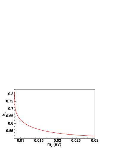
We can see that $k_{\nu}$ is the function of $m_{2}$ if $\Delta m_{\mathrm{sol}}^{2}$ and $\Delta m_{\mathrm{atm}}^{2}$ are fixed. Due to the inaccuracy of the experimental data, we take $\Delta m_{\mathrm{sol}}^{2}$ and $\Delta m_{\mathrm{atm}}^{2}$ as their best fit points here. The range of $k_{\nu}$ is shown in Fig. 1.

Figure 1: The range of $k_{\nu}$ of the normal mass scheme $m_{3}>m_{2}>m_{1}$.

We can see that $0.50<k_{\nu}<0.85$, and $k_{\nu}$ decreases with the increase of $m_{2}$. So $k_{\nu}<1$ for neutrinos. This is different from charged leptons.

2. For the inverted mass scheme, $m_{2}>m_{1}>m_{3}$, we have

$$k_{\nu}=\frac{\sqrt{m^{2}_{2}-\Delta m_{\mathrm{sol}}^{2}}+m_{2}+\sqrt{m^{2}_{2}-\Delta m_{\mathrm{atm}}^{2}}}{\frac{2}{3}\left(\sqrt[4]{m^{2}_{2}-\Delta m_{\mathrm{sol}}^{2}}+\sqrt{m_{2}}+\sqrt[4]{m^{2}_{2}-\Delta m_{\mathrm{atm}}^{2}}\right)^{2}}.$$ (10)

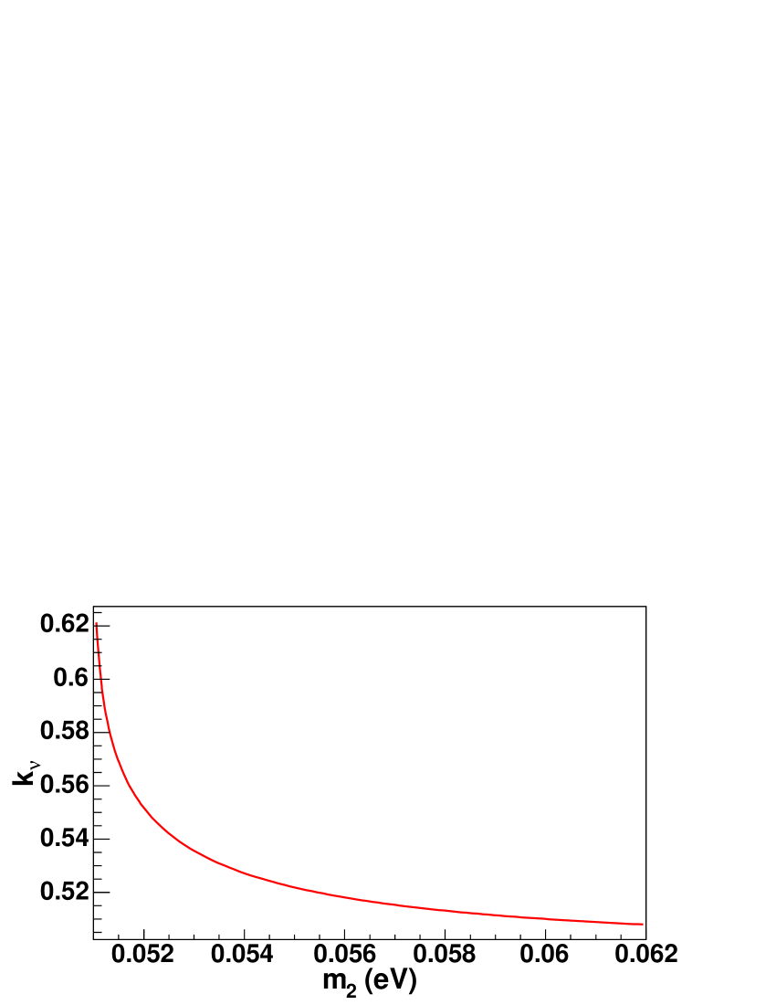
The range of $k_{\nu}$ is shown in Fig. 2.

Figure 2: The range of $k_{\nu}$ of the inverted mass scheme $m_{2}>m_{1}>m_{3}$.

We can see that $0.50<k_{\nu}<0.65$.

Altogether, $0.50<k_{\nu}<0.85$ for both these two mass schemes. And $k_{\nu}$ of the normal mass scheme is larger than that of the inverted mass scheme.

3. Koide’s relation for quarks

Now we turn to the cases of quarks. Because of the confinement of quarks, the inaccuracy of the masses of quarks is much bigger than that of leptons.

Here we take the data of PDG [4].

$$1.5~{}\mbox{MeV} <m_{u}< 4.5~{}\mbox{MeV},$$

$$1.0~{}\mbox{GeV} <m_{c}< 1.4~{}\mbox{GeV},$$

$$162.9~{}\mbox{GeV} <m_{t}< 188.5~{}\mbox{GeV},$$ (11)

$$5~{}\mbox{MeV} <m_{d}< 8.5~{}\mbox{MeV},$$

$$80~{}\mbox{MeV} <m_{s}< 155~{}\mbox{MeV},$$

$$4.0~{}\mbox{GeV} <m_{b}< 4.5~{}\mbox{GeV}.$$ (12)

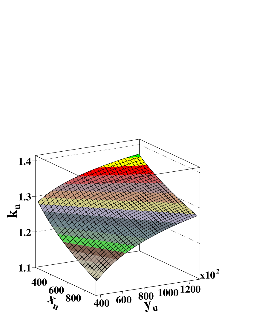
1. First, we calculate $k_{u}$ for $u$, $c$, $t$ quarks, i.e., u-type quarks,

$$k_{u} \equiv \frac{m_{u}+m_{c}+m_{t}}{\frac{2}{3}(\sqrt{m_{u}}+\sqrt{m_{c}}+\sqrt{m_{t}})^{2}}$$ (13)

$$= \frac{1+x_{u}+y_{u}}{\frac{2}{3}(1+\sqrt{x_{u}}+\sqrt{y_{u}})^{2}},$$

where $x_{u}=m_{c}/m_{u}$, $y_{u}=m_{t}/m_{u}$, and we can see that $k_{u}$ is the function only of the ratio of the masses of quarks. From Eq. (12), we get $2.2\times 10^{2}<x_{u}<9.3\times 10^{2}$ and $3.6\times 10^{4}<y_{u}<1.3\times 10^{5}$. Because Koide’s relation is not energy-scale invariant, the energy scale should be high energy where the current quark masses rather than the constituent quark masses should be adopted. The range of $k_{u}$ is shown in Fig. 3.

Figure 3: The range of $k_{u}$ for $u$, $c$, $t$ quarks.

We can see that $1.1<k_{u}<1.4$. Comparing with the cases of neutrinos, we find that $k_{u}>1$ for quarks, and $k_{\nu}<1$ for neutrinos.

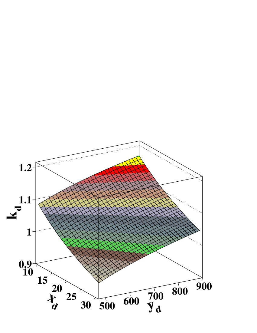
2. Second, we calculate $k_{d}$ for $d$, $s$, $b$ quarks, i.e., d-type quarks,

$$k_{d} \equiv \frac{m_{d}+m_{s}+m_{b}}{\frac{2}{3}(\sqrt{m_{d}}+\sqrt{m_{s}}+\sqrt{m_{b}})^{2}}$$ (14)

$$= \frac{1+x_{d}+y_{d}}{\frac{2}{3}(1+\sqrt{x_{d}}+\sqrt{y_{d}})^{2}},$$

where $x_{d}=m_{s}/m_{d}$, $y_{d}=m_{b}/m_{d}$. From Eq. (13), we get $9.4<x_{d}<31$ and $4.7\times 10^{2}<y_{d}<9.0\times 10^{2}$. The range of $k_{d}$ is shown in Fig. 4.

Figure 4: The range of $k_{d}$ for $d$, $s$, $b$ quarks.

We can see that $0.9<k_{d}<1.2$. Thus $k_{d}\approx 1$, and this is similar with the case of charged leptons.

Conclusively, the values of $k_{l}$, $k_{\nu}$, $k_{u}$ and $k_{d}$ can be summarized as follows

$$\left(\begin{array}[]{c}\nu_{e}\\ e\end{array}\right)\left(\begin{array}[]{c}\nu_{\mu}\\ \mu\end{array}\right)\left(\begin{array}[]{c}\nu_{\tau}\\ \tau\end{array}\right)\begin{array}[]{c}k_{\nu}<1\\ k_{l}=1\end{array},\mbox{and}\left(\begin{array}[]{c}u\\ d\end{array}\right)\left(\begin{array}[]{c}c\\ s\end{array}\right)\left(\begin{array}[]{c}t\\ b\end{array}\right)\begin{array}[]{c}k_{u}>1\\ k_{d}\approx 1\end{array}.$$ (15)

4. Estimate of the masses of neutrinos

We believe that the problem of the generation of the masses of leptons must be solved together with that of quarks. Since $k_{l}=1$ and $k_{d}\approx 1$, we may conjecture that $k_{l}+k_{d}\approx 2$. At the same time, since $0.50<k_{\nu}<0.85$ and $1.1<k_{u}<1.4$, we may analogize the conjecture of $k_{l}$ and $k_{d}$, and propose the hypothesis that

$$k_{\nu}+k_{u}\approx 2.$$ (16)

This is from the speculation that there must be some relation between $k_{l}$, $k_{\nu}$, $k_{u}$ and $k_{d}$. The situation seems to be similar to the quark-lepton complementarity between mixing angles of quarks and leptons [14], and we may call it a quark-lepton complementarity of masses.

Of course, this Ansatz is not the only one of the relations between $k_{l}$, $k_{\nu}$, $k_{u}$ and $k_{d}$. For example, we may also assume that $k_{l}k_{d}\approx k_{\nu}k_{u}\approx 1$, $k_{l}^{2}+k_{d}^{2}\approx k_{\nu}^{2}+k_{u}^{2}\approx 2$, or $\frac{1}{k_{l}}+\frac{1}{k_{d}}\approx\frac{1}{k_{\nu}}+\frac{1}{k_{u}}\approx 2$ (this is from the assumption that $\theta_{l}+\theta_{d}\approx\theta_{\nu}+\theta_{u}\approx\frac{\pi}{2}$ in Foot’s geometrical interpretation).

However, among all of these Ansätze, Eq. (17) is the simplest one, and it can show the balance between $k_{\nu}$ and $k_{u}$ (i.e., the quark-lepton complementarity) intuitively and transparently. Furthermore, the values of $k_{\nu}$ obtained under other Ansätze are close to the value obtained from Eq. (17), and the masses of neutrinos are not sensitive to the value of $k_{\nu}$ (we will show this in the following paragraphs), so we will use the hypothesis $k_{\nu}+k_{u}\approx 2$ here.

From Fig. 3, we can see that the mean value of $k_{u}$ is 1.25. Thus from the hypothesis $k_{\nu}+k_{u}\approx 2$, we get that $k_{\nu}\approx 0.75$. This is consistent with the normal mass scheme and in conflict with the inverted mass scheme. This indicates that the three masses of neutrinos mass eigenstates are heavier in order, which is the same as leptons and quarks.

Now we can estimate the absolute masses of neutrinos. Substituting $k_{\nu}=0.75$, $\Delta m_{\mathrm{atm}}^{2}=2.6\times 10^{-3}~{}\mbox{eV}^{2}$, and $\Delta m_{\mathrm{sol}}^{2}=6.9\times 10^{-5}~{}\mbox{eV}^{2}$ into Eq. (10), we can calculate the value of $m_{2}$,

$$0.75=\frac{\sqrt{m^{2}_{2}-6.9\times 10^{-5}~{}\mbox{eV}^{2}}+m_{2}+\sqrt{m^{2}_{2}+2.6\times 10^{-3}~{}\mbox{eV}^{2}}}{\frac{2}{3}\left(\sqrt[4]{m^{2}_{2}-6.9\times 10^{-5}~{}\mbox{eV}^{2}}+\sqrt{m_{2}}+\sqrt[4]{m^{2}_{2}+2.6\times 10^{-3}~{}\mbox{eV}^{2}}\right)^{2}},$$

and we get $m_{2}=8.4\times 10^{-3}~{}\mbox{eV}$.

Straightforwardly, we can get

$$m_{1}=\sqrt{m^{2}_{2}-\Delta m_{\mathrm{sol}}^{2}}=1.0\times 10^{-5}~{}\mbox{eV},$$ (17)

and

$$m_{3}=\sqrt{m^{2}_{2}+\Delta m_{\mathrm{atm}}^{2}}=0.05~{}\mbox{eV}.$$ (18)

From Eqs. (18)-(20), we can see that the masses of the neutrino mass eigenstates are of different orders of magnitude ($10^{-5}~{}\mbox{eV}$, $10^{-3}~{}\mbox{eV}$, and $10^{-2}~{}\mbox{eV}$), so they are hierarchical, and $m_{1}$ almost vanish because $m_{2}^{2}$ is very near $\Delta m_{\mathrm{sol}}^{2}$.

Now we can discuss the uncertainty of $m_{1}$, $m_{2}$ and $m_{3}$. In Fig. (1), we can see the slope of the curve in very large where $k_{\nu}\sim 0.75$, so the value of $m_{2}$ is not sensitive to the error of $k_{\nu}$. $m_{2}$ will approximately be $8.4\times 10^{-3}~{}\mbox{eV}$ even if the mean value of $k_{\nu}$ charges from 0.7 to 0.85, so the value of $m_{2}$ is precise to a good degree of accuracy. Similarly, the value of $m_{3}$ will be about $0.05~{}\mbox{eV}$ to a good degree of accuracy too, because $m_{3}=\sqrt{m^{2}_{2}+\Delta m_{\mathrm{atm}}^{2}}$, and $\Delta m_{\mathrm{atm}}^{2}\gg m^{2}_{2}$. The only point desired to be mentioned here is the range of $m_{1}$. Because $m^{2}_{2}$ is rather close to $\Delta m_{\mathrm{sol}}^{2}$, and due to the big uncertainty of $\Delta m_{\mathrm{sol}}^{2}$, the value of $m_{1}$ may change largely with $k_{\nu}$. The value $1.0\times 10^{-5}~{}\mbox{eV}$ is the rough estimate of the first step, and its effective number and order of magnitude may change with the more precise experimental data in the future.

Koide [15] also gave an interpretation of his relation as a mixing between octet and singlet components in a nonet scheme of the flavor $U(3)$. He also got the masses of neutrinos $m_{1}=0.0026~{}\mbox{eV}$, $m_{2}=0.0075~{}\mbox{eV}$ and $m_{3}=0.050~{}\mbox{eV}$ [16]. We can see that his results are strongly consistent with ours. Especially the values of $m_{2}$ and $m_{3}$ are almost the same (only with the exception of $m_{1}$, this is because $m^{2}_{2}$ is rather close to $\Delta m_{\mathrm{sol}}^{2}$, and the errors of $\Delta m_{\mathrm{sol}}^{2}$ is large in nowadays experimental data).

Now we calculate the effective masses of the three flavor eigenstares of neutrinos, which can be defined as

$$\langle m\rangle_{\alpha}\equiv\sqrt{\sum\limits_{i=1}^{3}\left(m_{i}^{2}|V_{\alpha i}|^{2}\right)},$$ (19)

where $\alpha=e,\mu,\tau$, and $V_{\alpha i}$ is the element of the neutrino mixing (MNS) matrix [17], which links the neutrino flavor eigenstates to the mass eigenstates. The best fit points of the modulus of MNS matrix are summarized as follows  [12]

$$|V|=\left(\begin{array}[]{ccc}0.84&0.54&0.08\\ 0.44&0.56&0.71\\ 0.32&0.63&0.71\\ \end{array}\right).$$ (20)

Then we get

$$\langle m\rangle_{e} = \sqrt{m_{1}^{2}|V_{e1}|^{2}+m_{2}^{2}|V_{e2}|^{2}+m_{3}^{2}|V_{e3}|^{2}}$$ (21)

$$= 6.0\times 10^{-3}~{}\mbox{eV}.$$

Similarly,

$$\langle m\rangle_{\mu}=3.6\times 10^{-2}~{}\mbox{eV},$$ (22)

$$\langle m\rangle_{\tau}=3.6\times 10^{-2}~{}\mbox{eV}.$$ (23)

The upper bounds of $\langle m\rangle_{e}$, $\langle m\rangle_{\mu}$ and $\langle m\rangle_{\tau}$ are measured by the experiments $\mbox{H}^{3}_{1}\rightarrow\mbox{He}^{3}_{2}+e+\overline{\nu}_{e}$, $\pi^{+}\rightarrow\mu^{+}+\nu_{\mu}$, and $\tau\rightarrow 5\pi+\nu_{\tau}$, respectively [4],

$$\langle m\rangle_{e} < 2.2~{}\mbox{eV},$$

$$\langle m\rangle_{\mu} < 0.19~{}\mbox{MeV},$$

$$\langle m\rangle_{\tau} < 18.2~{}\mbox{MeV}.$$ (24)

We can see that they are all consistent with the experimental data, and the more precise planed experiments (for example, KATRIN experiment [18]) will help to reach a higher sensitivity to test these results.

Furthermore, we can get the sum of the masses of the neutrino mass eigenstates,

$$\sum\limits_{i=1}^{3}m_{i}=0.058~{}\mbox{eV}.$$ (25)

This is also consistent with the data from cosmological observations (Wilkinson microwave anisotropy probe [19] and 2dF Galaxy Redshift Survey [20]),

$$\sum\limits_{i=1}^{3}m_{i}<0.71~{}\mbox{eV}.$$ (26)

All the analysis above shows the rationality of our results.

Also, $\langle m\rangle_{\mu}$ and $\langle m\rangle_{\tau}$ are almost the same because $m_{3}>m_{2}>m_{1}$, and thus the values of $\langle m\rangle_{\mu}$ and $\langle m\rangle_{\tau}$ are nearly only dominated by $m_{3}^{2}|V_{\mu 3}|^{2}$ and $m_{3}^{2}|V_{\tau 3}|^{2}$. However, $|V_{\mu 3}|^{2}\approx|V_{\tau 3}|^{2}\approx 0.71$, so $\langle m\rangle_{\mu}\approx\langle m\rangle_{\tau}$.

5. Summary

Finally, we give some discussion on our method in determining the masses of neutrinos. Although the reason and foundation of Koide’s relation is still unknown, there must be some deeper principle behind this elegant relation, and we believe that this relation must be applicable to neutrinos and quarks, at least to some degree. So we introduce the parameters $k_{\nu}$, $k_{u}$ and $k_{d}$ to describe the deviations of neutrinos and quarks from Koide’s relation. With this improved relation and the conjecture of a quark-lepton complementarity of masses such as $k_{l}+k_{d}\approx k_{\nu}+k_{u}\approx 2$, we can determine the absolute masses of the neutrino mass eigenstates and the effective masses of the neutrino flavor eigenstates. Due to the inaccuracy of the experimental data of neutrinos and quarks nowadays, these results should be only taken as primary estimates. However, if these results are tested to be consistent with more precise experiments in the future, it would be a big success of Koide’s relation, and we can get further understanding of the generation of the masses of leptons and quarks.

Acknowledgments

We are very grateful to Prof. Xiao-Gang He for his stimulating suggestions and valuable discussions. We also thank Yoshio Koide, Xun Chen, Xiaorui Lu, and Daxin Zhang for discussions. This work is partially supported by National Natural Science Foundation of China and by the Key Grant Project of Chinese Ministry of Education (NO. 305001).

References

[1]
A.O. Barut, Phys. Rev. Lett. 42 (1979) 1251.
[2]
Y. Koide, Lett. Nuovo Cimento 34 (1982) 201;
Y. Koide, Phys. Lett. B 120 (1983) 161.
[3]
Y. Koide, Phys. Rev. D 28 (1983) 252.
[4]
Particle Data Group, K. Hagiwara, et al., Phys. Rev. D 66 (2002) 010001.
[5]
R. Foot, hep-ph/9402242.
[6]
KamLAND Collaboration, K. Eguchi, et al., Phys. Rev. Lett. 90 (2003) 021802.
[7]
SNO Collaboration, S.N. Ahmad, et al., Phys. Rev. Lett. 92 (2004) 181301.
[8]
K2K Collaboration, M.H. Ahn, et al., Phys. Rev. Lett. 90 (2003) 041801.
[9]
Super-Kamiokande Collaboration, Y. Fukuda, et al., Phys.
Rev. Lett. 81 (1998) 1562; Y. Ashie, et al., Phys.
Rev. Lett. 93 (2004) 101801.
C.K. Jung, C. McGrew, T. Kajita, T. Mann, Anna. Rev. Nucl. Part.
Sci. 51 (2001) 451.
[10]
CHOOZ Collaboration, M. Apollonio, et al.,
Phys. Lett. B 420 (1998) 397;
Palo Verde Collaboration, F. Boehm, et al., Phys. Rev. Lett. 84 (2000) 3764.
[11]
M.C. Gonzalez-Garcia, hep-ph/0410030.
[12]
G. Altarelli, hep-ph/0410101.
[13]
S.P. Mikheyev, A.Yu. Smirnov, Sov. J. Nucl. Phys. 42 (1985) 913;
L. Wolfenstein, Phys. Rev. D 17 (1978) 2369.
[14]
M. Raidal, Phys. Rev. Lett. 93 (2004) 161801 (2004);
H. Minakata, A.Yu. Smirnov, Phys. Rev. D 70 (2004) 073009;
N. Li and B.-Q. Ma, hep-ph/0501226, Phys. Rev. D 71 (2005)
097301; hep-ph/0504161, EPJC, in press.
[15]
Y. Koide, M. Tanimoto, Z. Phys. C 72 (1996) 333.
[16]
Y. Koide, H. Nishiura, K. Matsuda, T. Kikuchi, T. Fukuyama,
Phys. Rev. D 66 (2002) 093006.
[17]
Z. Maki, M. Nakawaga, S. Sakata, Prog. Theor.
Phys. 28 (1962) 870.
[18]
KATRIN Project, A. Osipowicz, et al., hep-ex/0109033.
[19]
C.L. Bennett, Astrophys. J. Suppl. 148 (2003) 97;
D.N. Spergel, Astrophys. J. Suppl. 148 (2003) 175.
[20]
M. Colles, et al., Mon. Not. R. Astron. Soc. 328 (2001) 1039.