Abstract

In higher dimensional gauge theory, dynamics of non-Abelian Aharonov-Bohm phases induces gauge symmetry breaking through the Hosotani mechanism. Higgs fields in the four-dimensional spacetime are identified with the extra-dimensional components of the gauge fields. Basics of the Hosotani mechanism are reviewed, and applied to the electroweak theory. The Higgs boson mass and the Kaluza-Klein excitation scale are related to the weak $W$-boson mass.

28 April 2005 OU-HET 520/2005

Yutaka Hosotani

Department of Physics, Osaka University, Toyonaka, Osaka 560-0043, Japan

1.  Introduction

Gauge symmetry breaking is at the core of the current understanding of the particle interactions. Yet the Higgs particle remains as an enigma in the unified electroweak theory. Does it really exist? How heavy is it if it exists? How does it interact with quarks and leptons? These are the issues to be settled in the forthcoming experiments at LHC. In the standard model of electroweak interactions, the mass of Higgs bosons is in large part unconstrained. In the minimal supersymmetric standard model (MSSM) the mass of the lightest Higgs boson is predicted in the range 100 GeV to 130 GeV. The experimentally preferred value is $126^{+73}_{-48}\,$GeV. In this lecture we explore an alternative scenario, the dynamical gauge-Higgs unification, to try to pin down the nature of Higgs bosons.

In the dynamical gauge-Higgs unification formulated in a gauge theory in higher dimensions, extra-dimensional components of gauge fields play the role of Higgs fields in the four-dimensional spacetime.[1, 2, 3] When the extra-dimensional space is not simply connected, there appear non-Abelian Aharonov-Bohm phases, or Wilson line phases, whose fluctuation modes in the four dimensions serve as Higgs scalar fields. They are massless at the tree level. Its effective potential is completely flat at the classical level in the directions of Aharonov-Bohm phases, but becomes non-trivial at the quantum level. They may develop non-vanishing expectation values, thus inducing dynamical gauge symmetry breaking. This is called the Hosotani mechanism.[4, 5]

We first review the Hosotani mechanism to see how dynamics of Wilson line phases induce gauge symmetry breaking. Examples are given in $SU(N)$ gauge theory on $M^{n}\times S^{1}$. Then we explain how the scenario can be implemented in electroweak interactions by considering gauge theory on orbifolds. Detailed analysis is given in the $U(3)\times U(3)$ model on $M^{4}\times(T^{2}/Z_{2})$. The mass of the Higgs boson and the Kaluza-Klein mass scale is determined.

Part I. Dynamical gauge symmetry breaking by Wilson lines

2.  $SU(N)$ gauge theory on $M^{4}\times S^{1}$

If the space is not simply connected, Wilson line phases become physical degrees of freedom. Although constant Wilson line phases yield vanishing field strengths, they are dynamical and affect physics. At the classical level Wilson line phases label degenerate vacua. The degeneracy is lifted by quantum effects. The effective potential of Wilson line phases become non-trivial. If the effective potential is minimized at nontrivial values of Wilson line phases, then the rearrangement of gauge symmetry takes place. Spontaneous gauge symmetry breaking or enhancement is achieved dynamically.

Let us take $SU(N)$ gauge theory on $M^{4}\times S^{1}$ as an example. Let $x^{\mu}$ and $y$ be coordinates of $M^{4}$ and $S^{1}$, respectively. Points $y$ and $y+2\pi R$ are identified on $S^{1}$. Gauge theory is defined first on the covering space of $M^{4}\times S^{1}$, namely on $M^{4}\times R^{1}$, on which all fields are smooth. On $S^{1}$, physics must be the same at $y$ and $y+2\pi R$. However, it does not necessarily means that fields themselves are the same. Upon a loop translation along $S^{1}$, each field needs to come back to the original value up to a (global) gauge transformation.

$$\hskip-28.45274ptA_{M}(x,y+2\pi R)=UA_{M}(x,y)\,U^{\dagger}~{}~{}~{},$$ (2.1)

$$\hskip-28.45274pt\psi(x,y+2\pi R)=e^{i\beta}\,T[U]\psi(x,y)~{}~{}~{}~{}.$$ (2.2)

$U$ is an element of $SU(N)$. $T[U]\psi=U\psi$ or $U\psi U^{\dagger}$ for $\psi$ in the fundamental or adjoint representation, respectively. The boundary condition (2.2) guarantees that the physics is the same at $(x,y)$ and $(x,y+2\pi R)$. The theory is defined with a set of boundary conditions $\{U,\beta\}$.

One might ask the following questions. Does $U\not\propto I$ imply symmetry breaking? What is the symmetry of the theory for a general $U$? Answers to these questions are quite nontrivial. Under a gauge transformation

$$A_{M}^{\prime}=\Omega\bigg{(}A_{M}-{i\over g}\partial_{M}\bigg{)}\Omega^{\dagger}~{}~{},$$ (2.3)

$A_{M}^{\prime}$ obeys a new set of boundary conditions

$$\hskip-28.45274ptA_{M}^{\prime}(x,y+2\pi R)=U^{\prime}A_{M}^{\prime}(x,y)\,U^{\prime\dagger}~{}~{}~{},$$ (2.4)

$$\hskip-28.45274ptU^{\prime}=\Omega(x,y+2\pi R)\,U\,\Omega(x,y)^{\dagger}~{},$$ (2.5)

provided $\partial_{M}U^{\prime}=0$. The set $\{U^{\prime},\beta\}$ can be different from the set $\{U,\beta\}$. When the relation $\partial_{M}U^{\prime}=0$ is satisfied, we write

$$\{U^{\prime},\beta\}~{}\sim~{}\{U,\beta\}~{}~{}.$$ (2.6)

The relation is transitive, and therefore is an equivalence relation. Sets of boundary conditions form equivalence classes of boundary conditions with respect to the equivalence relation (2.6).[5] As an example we note

$$U=\pmatrix{e^{i\alpha_{1}}\cr&\cdots\cr&&e^{i\alpha_{N}}} \Omega=\pmatrix{e^{i\gamma_{1}y/2\pi R}\cr&\cdots\cr&&e^{i\gamma_{N}y/2\pi R}}$$ , (2.7)

$$\Rightarrow U^{\prime}=\pmatrix{e^{i(\alpha_{1}+\gamma_{1})}\cr&\cdots\cr&&e^{i(\alpha_{N}+\gamma_{N})}}~{}~{}.$$ (2.8)

Although the theories defined with $\{U,\beta\}$ and $\{U^{\prime},\beta\}$ seem different, they should be equivalent and should have the same physics as they are related to each other by a “large gauge transformation”.

The equivalence of physics is guaranteed by the dynamics of Wilson line phases. Take a theory with the boundary conditions (2.2). Given $U$, there are zero modes ($(x^{\mu},y)$-independent modes) of $A_{y}$ satisfying $[A_{y},U]=0$. Although they give vanishing field strengths, they cannot be gauged away in general. Indeed, eigenvalues $\{e^{i\theta_{1}},\cdots,e^{i\theta_{N}}\}$ of $P\exp\Big{(}ig\int_{0}^{2\pi R}dy\,A_{y}\Big{)}\cdot U$ are invariant under all gauge transformations preserving the boundary conditions (2.2). $\{\theta_{1},\cdots,\theta_{N}\}$ are the Wilson line phases. They are non-Abelian Aharonov-Bohm phases.

The effective potential for $\{\theta_{1},\cdots,\theta_{N}\}$ becomes nontrivial at the quantum level. At the one loop level

$$V_{\rm eff}[\theta_{W}]^{d=5}=\sum(\mp){\displaystyle i\over\displaystyle 2}\,{\rm tr}\,\ln D_{M}D^{M}$$ (2.9)

where $D_{M}D^{M}=\partial_{\mu}\partial^{\mu}-D_{y}^{2}$. $D_{y}$ stands for a covariant derivative with a constant $A_{y}$ yielding $\theta_{W}$’s. The sign is $-$ ($+$) for a boson (fermion). Given the boundary conditions and background $A_{y}$, the spectrum of each field is determined. On $S^{1}$ the spectrum in the $y$-direction takes the form $[n+\gamma(\theta_{W})]^{2}/R^{2}$ where $n$ runs over integers. Here $\gamma(\theta_{W})$ depends on the boundary conditions and couplings of the fields. It satisfies that $\gamma(\theta_{W}+2\pi)=\gamma(\theta_{W})+\ell$ where $\ell$ is an integer. Hence, after making a Wick rotation, the four-dimensional $V_{\rm eff}$ becomes

$$\hskip-28.45274ptV_{\rm eff}[\theta_{W}]=(2\pi R)\cdot V_{\rm eff}[\theta_{W}]^{d=5}$$ (2.10)

$$\hskip 14.22636pt=\sum(\pm){\displaystyle 1\over\displaystyle 2}\int{\displaystyle d^{4}p_{E}\over\displaystyle(2\pi)^{4}}\sum_{n=-\infty}^{\infty}\ln\bigg{\{}p_{E}^{2}+{\displaystyle[n+\gamma(\theta_{W})]^{2}\over\displaystyle R^{2}}\bigg{\}}~{}~{}.$$ (2.11)

As will be proven in the next section, the $\theta_{W}$-dependent part of $V_{\rm eff}[\theta_{W}]$ is finite. It is given by

$$\hskip-28.45274ptV_{\rm eff}[\theta_{W}]=\sum(\mp){\displaystyle 3\over\displaystyle 64\pi^{6}R^{4}}~{}h_{5}[\gamma(\theta_{W})]+{\rm constant}~{},$$ (2.12)

$$\hskip-17.07182pth_{d}(x)=\sum_{n=1}^{\infty}{\displaystyle\cos 2\pi nx\over\displaystyle n^{d}}~{}~{}.$$ (2.13)

The effective potential has a global minimum at $\theta_{W}=\theta_{W}^{\rm min}$, depending on the content of matter fields. When $\theta_{W}^{\rm min}\not=0$, the physical symmetry of the theory differs from the symmetry determined by the boundary condition matrix $U$ in (2.2). To find the physical symmetry it is most convenient to make a general gauge transformation which alters boundary conditions. Let $A_{y}^{\rm min}$ be the constant gauge potential corresponding to $\theta_{W}^{\rm min}$. It follows from (2.2) that $[A_{y}^{\rm min},U]=0$. We perform a gauge transformation (2.3) with $\Omega(y)=\exp\big{\{}igyA_{y}^{\rm min}\big{\}}$. In the new gauge the boundary condition matrix changes to $U^{\prime}=U\exp\big{\{}2\pi igRA_{y}^{\rm min}\big{\}}\equiv U^{\rm sym}$ as specified in (2.5). Since the effective potential is minimized at $A_{y}^{\prime}=0$, the physical symmetry is given by the symmetry specified with $U^{\rm sym}$.

3.  Finiteness of $V_{\rm eff}[\theta_{W}]$

Although gauge theory in higher dimensions is not renormalizable, the $\theta_{W}$-dependent part of the effective potential can be evaluated unambiguously. It turns out finite at the one loop level, being free from divergences which may sensitively depend on physics at much higher energy scales. The $\theta_{W}$-dependent parts of all physical quantities might finite.[6] In this section we show how (2.13) is derived, and present theorems.

Consider a quantity

$$f(x)={\displaystyle 1\over\displaystyle 2}\int{\displaystyle d^{d}q_{E}\over\displaystyle(2\pi)^{d}}\sum_{n=-\infty}^{\infty}\ln\big{\{}q_{E}^{2}+(n+x)^{2}\big{\}}~{}~{}.$$ (3.1)

The $x$-dependent part of $f(x)$ is easily found by the zeta function regularization. Associated with $f(x)$, $\zeta(s;x)$ is defined by

$$\zeta(s;x)={\displaystyle 1\over\displaystyle 2}\int{\displaystyle d^{d}q_{E}\over\displaystyle(2\pi)^{d}}\sum_{n=-\infty}^{\infty}\Big{\{}q_{E}^{2}+(n+x)^{2}\Big{\}}^{-s}\quad{\rm for~{}}\Re\,s>{\displaystyle d+1\over\displaystyle 2}~{}.$$ (3.2)

For $\Re\,s\leq\hbox{${1\over 2}$}(d+1)$, $\zeta(s;x)$ is defined by analytic continuation. $f(x)$ is, then, given by

$$f(x)=-\zeta^{\prime}(0;x)~{}~{}.$$ (3.3)

Making use of

$$\hskip-28.45274pt{\displaystyle 1\over\displaystyle A^{s}}={\displaystyle 1\over\displaystyle\Gamma(s)}\int_{0}^{\infty}dt\,t^{s-1}\,e^{-At}~{}~{},$$ (3.4)

$$\hskip-28.45274pt\sum_{n=-\infty}^{\infty}e^{-t(n+x)^{2}}=\bigg{(}{\displaystyle\pi\over\displaystyle t}\bigg{)}^{1/2}\sum_{n=-\infty}^{\infty}e^{-\pi^{2}n^{2}/t+2\pi inx}~{}~{},$$ (3.5)

$\zeta(s;x)$ is transformed to

$$\hskip-28.45274pt\zeta(s;x)={\displaystyle 1\over\displaystyle\Gamma(s)}\int_{0}^{\infty}dt\,t^{s-1}\,{\displaystyle 1\over\displaystyle 2}\int{\displaystyle d^{d}q_{E}\over\displaystyle(2\pi)^{d}}\sum_{n=-\infty}^{\infty}e^{-[\,q_{E}^{2}+(n+x)^{2}\,]\,t}$$ (3.6)

$$\hskip 5.69046pt={\displaystyle 1\over\displaystyle\Gamma(s)}{\displaystyle 1\over\displaystyle 2^{d+1}\pi^{(d-1)/2}}\int_{0}^{\infty}dt\,t^{s-1-(d+1)/2}\sum_{n=-\infty}^{\infty}e^{-\pi^{2}n^{2}/t+2\pi inx}~{}.$$ (3.7)

The $n=0$ term in the last line is independent of $x$. Hence

$$\hskip-28.45274ptf(x)=-{\displaystyle 1\over\displaystyle 2^{d+1}\pi^{(d-1)/2}}\int_{0}^{\infty}dt\,t^{-1-(d+1)/2}\sum_{n\not=0}e^{-\pi^{2}n^{2}/t+2\pi inx}+{\rm constant}$$ (3.8)

$$\hskip 5.69046pt=-{\displaystyle\Gamma\Big{(}\hbox{${1\over 2}$}(d+1)\Big{)}\over\displaystyle 2^{d}\pi^{(3d+1)/2}}~{}h_{d+1}(x)+{\rm constant}~{}~{}.$$ (3.9)

The formula (3.9) with $d=4$ leads to (2.13).

$h_{d}(x)$ is periodic; $h_{d}(x+1)=h_{d}(x)$. It is, in general, singular at $x=$an integer. For examples,

$$\hskip-28.45274pth_{2}(x)=\pi^{2}(x-\hbox{${1\over 2}$})^{2}-{\displaystyle\pi^{2}\over\displaystyle 12}~{}~{},$$ (3.10)

$$\hskip-28.45274pth_{4}(x)=-{\displaystyle\pi^{4}\over\displaystyle 3}(x-\hbox{${1\over 2}$})^{4}+{\displaystyle\pi^{4}\over\displaystyle 6}(x-\hbox{${1\over 2}$})^{2}-{\displaystyle 7\pi^{4}\over\displaystyle 720}~{}~{},$$ (3.11)

for $0\leq x\leq 1$. It is easy to see

$$h_{2}^{\prime\prime}(x)=2\pi^{2}\Big{\{}1-\delta_{1}(x)\Big{\}}$$ (3.12)

where $\delta_{a}(x)=\sum_{n}\delta(x-an)$. For even $d\geq 4$, $h_{d}^{(d-2)}(x)=(2\pi)^{d-2}(-1)^{(d-2)/2}h_{2}(x)$ so that $h_{d}(x)$ has a singularity of cusp type at $x=n$ ($n$: an integer).

The behavior of $h_{d}(x)$ for odd $d$ is slightly different. Recall

$$\hskip-28.45274pth_{1}(x)=-\ln\Big{(}2\sin\pi x\Big{)}\qquad{\rm for~{}}0<x<1~{},$$ (3.13)

$$\hskip-28.45274pth_{1}^{\prime}(x)=-{\displaystyle\pi\over\displaystyle 2}\cot\pi x~{}~{}.$$ (3.14)

Hence $h_{d}(x)$ has singular behavior at $x=0$ as $x^{d-1}\ln|x|$ for odd $d$.

The $\theta_{W}$-dependent part of the effective potential $V_{\rm eff}$ turns out finite. We summarize it in a theorem.

Theorem

   The effective potential for the Wilson line phases, $V_{\rm eff}(\theta_{W})$, is finite at the one loop level apart from a $\theta_{W}$-independent constant term.   

(Proof)  In general there are several Wilson line phases, $\theta_{j}$ ($j=1,\cdots,p$). The proof is given for $p=1$, but can be generalized to arbitrary $p$. We assume that every quantity can be regularized in a gauge invariant manner as in the dimensional regularization method. Thanks to the invariance under large gauge transformations, $V_{\rm eff}(\theta_{W})$ is periodic in $\theta_{W}$ with a period $2\pi$. Thus its Fourier expansion is written as

$$V_{\rm eff}(\theta_{W})=\sum_{n=-\infty}^{\infty}a_{n}e^{in\theta_{W}}~{}.$$ (3.15)

The equality is understood as the convergence in the $L^{2}$ norm. $a_{0}$ may be divergent. The theorem claims that $V_{\rm eff}(\theta_{W})-a_{0}$ is finite at the one loop level.

Indeed, the effective action at the one loop level can be written in the form

$$\hskip-28.45274ptV_{\rm eff}(\theta_{W})^{\rm 1~{}loop}=\sum_{j}\hat{f}[\ell_{j}\theta_{W}+c_{j};m_{j}^{2}]~{}~{},$$ (3.16)

$$\hskip-28.45274pt\hat{f}(\theta;m^{2})={\displaystyle 1\over\displaystyle 2}\int{\displaystyle d^{d}q_{E}\over\displaystyle(2\pi)^{d}}\sum_{n=-\infty}^{\infty}\ln\bigg{\{}q_{E}^{2}+\bigg{(}n+{\displaystyle\theta\over\displaystyle 2\pi}\bigg{)}^{2}+m^{2}\bigg{\}}~{}~{},$$ (3.17)

where $\ell_{j}$ and $c_{j}$ are an integer and a constant, respectively. $\hat{f}(\theta;0)=f(\theta/2\pi)$ has been explicitly evaluated above with the result (3.9) which gives a finite contribution to $V_{\rm eff}(\theta_{W})-a_{0}$.

The argument can be generalized for $\hat{f}(\theta;m^{2})$ with $m^{2}>0$. By differentiating $\hat{f}$ $d+2$ times with respect to $\theta$, the integral and the infinite sum becomes convergent at all $\theta$ for $m^{2}>0$, giving finite $\hat{f}^{(d+2)}$. By integrating and making use of $\int_{0}^{2\pi}d\theta\,\hat{f}^{(k)}=0$ $(k=1,\cdots,d-1)$, the finiteness of the $\theta$-dependent part of $\hat{f}(\theta;m^{2})$ is shown. $\diamondsuit$

When $m^{2}=0$, the differentiation of $\hat{f}(\theta;m^{2})$ leads to infrared divergence at $\theta=0$ ($mod~{}2\pi$). One generalizes the theorem.

Conjecture

   The $\theta_{W}$-dependent part of $V_{\rm eff}(\theta_{W})$ is finite almost everywhere to every order in perturbation theory.   

(Outline of proof)  There are massless particles whose propagators $D$ take the form $D^{-1}=p_{E}^{2}+(n+\gamma(\theta_{W}))^{2}/R^{2}$. $D^{-1}$ can vanish only when $\gamma(\theta_{W})$ is an integer. A point $\theta_{W}$ is said to be regular if $\gamma(\theta_{W})$ is not an integer.

Corrections to $V_{\rm eff}(\theta_{W})$ at the higher loop levels are written as integrals of bubble diagrams. There are only a finite number of diagrams in each order in perturbation theory. $\theta_{W}$ appears in vertices in power, and in propagators $D^{-1}$. Hence, by differentiating the diagrams with respect to $\theta_{W}$ at regular points sufficiently many times, the integrals become convergent. The integrals can diverge only at a finite number of points in $0\leq\theta_{W}<2\pi$. By integration each diagram gives a finite contribution to the $\theta_{W}$-dependent part of $V_{\rm eff}(\theta_{W})$ at regular points. $\diamondsuit$

4.  Dynamical gauge symmetry breaking

Let us consider $SU(N)$ gauge theory on $M^{4}\times S^{1}$ with fermions in the fundamental and adjoint representations. It can be shown that all $U$ in (2.2) are in one equivalence class of boundary conditions, that is, the theory with $\{U,\beta\}$ is equivalent with the theory with $\{I,\beta\}$ on $M^{4}\times S^{1}$.

Without loss of generality we take $U=I$. Gauge fields are periodic on $S^{1}$. Wilson line phases are related to the zero modes of $A_{y}$:

$$A_{y}=\sum_{a=1}^{N^{2}-1}\hbox{${1\over 2}$}A_{y}^{a}\lambda^{a}={\displaystyle 1\over\displaystyle 2\pi gR}\pmatrix{\theta_{1}\cr&\ddots\cr&&\theta_{N}\cr}$$ (4.1)

where $\sum_{j=1}^{N}\theta_{j}=0$. The four-dimensional effective potential is given by

$$\hskip-28.45274ptV_{\rm eff}(\theta)=C\Bigg{\{}-3\sum_{j,k=1}^{N}h_{5}\bigg{(}{\displaystyle\theta_{j}-\theta_{k}\over\displaystyle 2\pi}\bigg{)}+4N_{\rm fund}^{F}\sum_{j=1}^{N}h_{5}\bigg{(}{\displaystyle\theta_{j}-\beta_{\rm fund}\over\displaystyle 2\pi}\bigg{)}$$ (4.2)

$$\hskip 113.81102pt+4N_{\rm ad}^{F}\sum_{j,k=1}^{N}h_{5}\bigg{(}{\displaystyle\theta_{j}-\theta_{k}-\beta_{\rm ad}\over\displaystyle 2\pi}\bigg{)}~{}\Bigg{\}}~{}~{},$$ (4.3)

$$\hskip 0.0ptC={\displaystyle 3\over\displaystyle 4\pi^{2}}{\displaystyle 1\over\displaystyle(2\pi R)^{4}}~{}.$$ (4.4)

Here $N_{\rm fund}^{F}$ and $N_{\rm ad}^{F}$ are the numbers of fermion multiplets in the fundamental and adjoint representations, respectively. $\beta_{\rm fund}$ and $\beta_{\rm ad}$ are the boundary condition parameters appearing in (2.2). In general, each multiplet of fermions can have distinct $\beta$.

Theorem

   In pure $SU(N)$ gauge theory on $M^{4}\times S^{1}$, $SU(N)$ gauge symmetry is unbroken.   

(Proof)  This follows immediately from (4.4) with $N^{F}_{\rm fund}=N^{F}_{\rm ad}=0$. $V_{\rm eff}$ is minimized when $\theta_{j}=\theta_{k}$ for all $j$ and $k$. As $\sum_{j=1}^{N}\theta_{j}=0$ ($mod~{}2\pi$), there are $N$ degenerate minima where $\theta_{j}=\theta_{k}=0,2\pi/N,4\pi/N,\cdots$. It can be shown that in pure $SU(N)$ gauge theory on $M^{4}\times T^{n}$, $SU(N)$ gauge symmetry is unbroken.

The presence of other matter fields can change the situation. We list a few examples in $SU(3)$ gauge theory. In pure gauge theory there are three degenerate minima. See fig. 1(a). We add fermions to see what happens.

(i) $N^{F}_{\rm fund}>0$ and $N^{F}_{\rm ad}=0$

If all fermions are in the fundamental representation and have common $\beta$, then the $SU(3)$ symmetry remains unbroken. The global minimum of $V_{\rm eff}$ is located at

$$(\theta_{1},\theta_{2})=\cases{(-{2\over 3}\pi,-{2\over 3}\pi)&for $0<\beta<{2\over 3}\pi$,\cr\kern 5.0pt\cr(0,0)&for ${2\over 3}\pi<\beta<{4\over 3}\pi$,\cr\kern 5.0pt\cr(+{2\over 3}\pi,+{2\over 3}\pi)&for ${4\over 3}\pi<\beta<2\pi$.\cr}$$ (4.5)

See fig. 1(b).

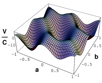
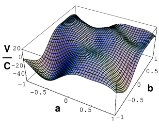
(a)                                                             (b)

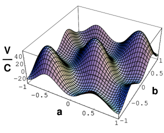
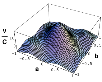
(c)                                                             (d)

Figure 1: The effective potential $V_{\rm eff}(\theta_{1},\theta_{2})$ in the $SU(3)$ gauge theory on $M^{4}\times S^{1}$. $(\theta_{1},\theta_{2})=(\pi a,\pi b)$. (a) In pure gauge theory. There are three degenerate minima. (b) $(N^{F}_{\rm fund},N^{F}_{\rm ad})=(3,0)$. $\beta=0.3\pi$. The global minimum is located at $(\theta_{1},\theta_{2})=(-{2\over 3}\pi,-{2\over 3}\pi)$. (c) $(N^{F}_{\rm fund},N^{F}_{\rm ad})=(0,1)$. $\beta=0$. The global minimum is located at $(\theta_{1},\theta_{2})=(\pm{2\over 3}\pi,\mp{2\over 3}\pi),(0,\pm{2\over 3}\pi),(\pm{2\over 3}\pi,0)$, which correspond to $U(1)\times U(1)$ symmetry. (d) $(N^{F}_{\rm fund},N^{F}_{\rm ad})=(1,1)$. $\beta=0$. $\beta=0.3\pi$. The global minimum is located at $(\theta_{1},\theta_{2})=(\pi,\pi),(0,\pi),(\pi,0)$, which correspond to $SU(2)\times U(1)$ symmetry.

(ii) $N^{F}_{\rm fund}=0$ and $N^{F}_{\rm ad}>0$

Suppose that all fermions belong to the adjoint representation and have $\beta=0$. In this case there are six degenerate minima. The location $(\theta_{1},\theta_{2},\theta_{3})$ is given by a permutation of $(0,{2\over 3}\pi,-{2\over 3}\pi)$. $SU(3)$ symmetry breaks down to $U(1)\times U(1)$. See fig. 1(c).

(iii) $N^{F}_{\rm fund}=N^{F}_{\rm ad}=1$

Suppose that there exist fermions in the fundamental representation and in the adjoint representation. In particular, consider the case $N^{F}_{\rm fund}=N^{F}_{\rm ad}=1$ with $\beta=0$. As depicted in fig. 1(d), the global minima are located at $(\theta_{1},\theta_{2},\theta_{3})=(0,\pi,\pi),(\pi,0,\pi),(\pi,\pi,0)$. The physical symmetry is $SU(2)\times U(1)$.

We have seen that dynamical gauge symmetry breaking takes place in the cases (ii) and (iii). From the four-dimensional viewpoint the extra-dimensional components of gauge fields play the role of Higgs fields in four dimensions. When Wilson line phases develop non-trivial vacuum expectation values by quantum effects, gauge symmetry is spontaneously broken.

Dynamics of Wilson line phases are summarized as follows.

   Hosotani mechanism
  In gauge theory defined on a non-simply connected space, a configuration with vanishing field strengths is not necessarily a pure gauge. There are non-Abelian Aharonov-Bohm phases, or Wilson line phases ($\theta_{j}$), which become physical degrees of freedom.
(i) $\raise 0.68889pt\hbox{$\langle$}\lower 0.68889pt\hbox{}\theta_{j}\,\raise 0.68889pt\hbox{$\rangle$}\lower 0.68889pt\hbox{}$ is dynamically determined.
(ii) When $\raise 0.68889pt\hbox{$\langle$}\lower 0.68889pt\hbox{}\theta_{j}\,\raise 0.68889pt\hbox{$\rangle$}\lower 0.68889pt\hbox{}$ is nontrivial, gauge symmetry is dynamically broken at the quantum level.
(iii) Higgs fields in four dimensions are unified with gauge fields.
(iv) Physics is the same within each equivalence class of boundary conditions.   

We add a comment. In supersymmetric theories the effective potential $V_{\rm eff}(\theta)$ vanishes if supersymmetry remains exact and unbroken, as there is cancellation among contributions from bosons and fermions. When supersymmetry is broken either spontaneously or softly, then $V_{\rm eff}(\theta)$ becomes nontrivial. Thus supersymmetry breaking can induce dynamical gauge symmetry breaking, as was first clarified by Takenaga.[7]

Part II. Dynamical gauge symmetry breaking in the
electroweak theory

5.  Electroweak gauge-Higgs unification on orbifolds

There are two important ingredients to be implemented in applying the scheme of dynamical gauge-Higgs unification to the electroweak interactions. First of all the electroweak symmetry is $SU(2)_{L}\times U(1)_{Y}$, which is broken to $U(1)_{EM}$. In the standard electroweak theory the Higgs field in an $SU(2)_{L}$ doublet induces the symmetry breaking. In the scheme of dynamical gauge-Higgs unification explained in the Part I, Higgs fields in four dimensions are identified with the extra-dimensional components of gauge fields which necessarily belong to the adjoint representation of the gauge group. Thus the Higgs doublet in the electroweak theory must be a part of the field in the adjoint representation of a larger group, as was first clarified by Fairlie[2] and by Forgacs and Manton.[3] The enlarged gauge group has to contain either $SU(3)$, $SO(5)$, or $G_{2}$.

Secondly fermions are chiral in the electroweak theory. The most economical and powerful way of having chiral fermions in four dimensions is to start a gauge theory on orbifolds.[8] The orbifold projection makes the fermion content chiral.

Many models have been proposed in the literature.[8]-[19] As an extra-dimensional space, $S^{1}/Z_{2}$ and $T^{2}/Z_{2}$ have been most commonly considered. Gauge theory on the Randall-Sundrum warped spacetime has been intensively investigated, as well.

Let us consider $SU(N)$ gauge theory on $M^{4}\times(T^{n}/Z_{2})$ with coordinates $x^{\mu}$ ($\mu=0,\cdots,3$) and $y^{a}$ $(a=1,\cdots,n)$.[17] $T^{n}/Z_{2}$ is obtained by the identification

$$T_{a} : \vec{y}+\vec{l}_{a}~{}\sim~{}\vec{y}$$ (5.2)

$$\vec{l}_{a}=(0,\cdots,2\pi R_{a},\cdots,0)~{}~{}~{}(a=1,2,\cdots,n)~{},$$

$$Z_{2} : -\vec{y}~{}\sim~{}\vec{y}~{}~{}~{}.$$ (5.3)

As $T^{n}$ is not simply connected, there appear Wilson line phases as physical degrees of freedom as explained in Part I. In the course of the $Z_{2}$ orbifolding there appear fixed points. Theory requires additional boundary conditions at those fixed points, which gives us benefit of eliminating some of light modes in various fields. Chiral fermions naturally appear at low energies. Some of Wilson line phases drop out from the spectrum, while the others survive. The surviving Wilson line phases play the role of Higgs fields in $M^{4}$, inducing dynamical gauge symmetry breaking.

Although $(x,\vec{y})$ and $(x,\vec{y}+\vec{l}_{a})$ represent the same point on $T^{n}$, the values of fields need not be the same. In general

$$\hskip-28.45274ptA_{M}(x,\vec{y}+\vec{l}_{a})=U_{a}A_{M}(x,\vec{y})\,U_{a}^{\dagger}~{}~{}~{},$$ (5.4)

$$\hskip-28.45274pt\psi(x,\vec{y}+\vec{l}_{a})=\eta_{a}\,T[U_{a}]\psi(x,\vec{y})~{}~{}~{},$$ (5.5)

$$\hskip-28.45274pt[U_{a},U_{b}]=0~{}~{}~{},~{}~{}~{}U_{a}\in SU(N)~{}~{}~{}(a,b=1,\cdots,n)~{}.$$ (5.6)

$\eta_{a}$ is a $U(1)$ phase factor. $T[U_{a}]\psi=U_{a}\psi$ or $U_{a}\psi U_{a}^{\dagger}$ for $\psi$ in the fundamental or adjoint representation, respectively. The boundary condition (5.6) guarantees that the physics is the same at $(x,\vec{y})$ and $(x,\vec{y}+\vec{l}_{a})$. The condition $[U_{a},U_{b}]=0$ is necessary to ensure $T_{a}T_{b}=T_{b}T_{a}$.

Similar conditions follow from the $Z_{2}$ orbifolding: $Z_{2}~{}:~{}-\vec{y}~{}\sim~{}\vec{y}$. On $T^{n}$, this parity operation allows fixed points at $z$ where the relation $\vec{z}=-\vec{z}+\sum_{a}m_{a}\vec{l}_{a}$ ($m_{a}=$ an integer) is satisfied. There appear $2^{n}$ fixed points on $T^{n}$. Combining it with loop translations in (5.6), one finds that parity around each fixed point is also symmetry:

$$Z_{2,j}~{}:~{}\vec{z}_{j}-\vec{y}~{}\sim~{}\vec{z}_{j}+\vec{y}\quad(j=0,\cdots,2^{n}-1)~{}~{}~{}.$$ (5.7)

Accordingly fields must satisfy additional boundary conditions.

Let spacetime be $M^{4}\times(T^{2}/Z_{2})$, in which case $\vec{z}_{0}=(0,0)$, $\vec{z}_{1}=(\pi R_{1},0)$, $\vec{z}_{2}=(0,\pi R_{2})$, and $\vec{z}_{3}=(\pi R_{1},\pi R_{2})$. Under $Z_{2,j}$ in (5.7)

$$\hskip-28.45274pt\pmatrix{A_{\mu}\cr A_{y_{a}}\cr}(x,\vec{z}_{j}-\vec{y})=P_{j}\pmatrix{A_{\mu}\cr-A_{y_{a}}\cr}(x,\vec{z}_{j}+\vec{y})\,P_{i}^{\dagger}~{}~{},$$ (5.8)

$$\hskip-28.45274pt\psi(x,\vec{z}_{j}-\vec{y})=\eta_{j}^{\prime}\,T[P_{j}]\,(i\Gamma^{4}\Gamma^{5})\psi(x,\vec{z}_{j}+\vec{y})\qquad(\eta_{j}^{\prime}=\pm 1)$$ (5.9)

$$\hskip-28.45274pt\qquad(a=1,2,\quad j=0,1,2,3)~{}~{}.$$ (5.10)

Here $P_{j}=P_{j}^{-1}=P_{j}^{\dagger}\in SU(N)$. Not all $U_{a}$’s and $P_{j}$’s are independent. On $T^{2}/Z_{2}$, only three of them are independent. One can show that

$$\hskip-28.45274ptU_{a}=P_{a}P_{0}~{}~{}~{},~{}~{}~{}P_{3}=P_{2}P_{0}P_{1}=P_{1}P_{0}P_{2}~{}~{}~{},$$ (5.11)

$$\hskip-28.45274pt\eta_{a}=\eta_{0}^{\prime}\eta_{a}^{\prime}=\pm 1\quad(a=1,2)~{}.$$ (5.12)

Gauge theory on $M^{4}\times(T^{2}/Z_{2})$ is specified with a set of boundary conditions $\{P_{j},\eta_{j}^{\prime}~{};~{}j=0,1,2\}$. If fermions $\psi$ in (5.10) are 6-D Weyl fermions, i.e. $\Gamma^{7}\psi=+\psi$ or $-\psi$ where $\Gamma^{7}=\Gamma^{0}\cdots\Gamma^{5}$, then the boundary condition (5.10) makes 4D fermions chiral.

At a first look, the original gauge symmetry is broken by the boundary conditions if $P_{0}$, $P_{1}$ and $P_{2}$ are not proportional to the identity matrix. This part of the symmetry breaking is often called the orbifold symmetry breaking in the literature. However, the physical symmetry of the theory can be different from the symmetry of the boundary conditions, and different sets of boundary conditions can be equivalent to each other.

6.  The Hosotani mechanism on orbifolds

It is important to recognize that sets of boundary conditions form equivalence classes. As in (2.5), under a gauge transformation (2.3) $A_{M}^{\prime}$ obeys a new set of boundary conditions $\{P_{j}^{\prime},U_{a}^{\prime}\}$ where

$$\hskip-28.45274ptP_{j}^{\prime}=\Omega(x,\vec{z}_{j}-\vec{y})\,P_{j}\,\Omega(x,\vec{z}_{j}+\vec{y})^{\dagger}~{},$$ (6.1)

$$\hskip-28.45274ptU_{a}^{\prime}=\Omega(x,\vec{y}+\vec{l}_{a})\,U_{a}\,\Omega(x,\vec{y})^{\dagger}~{},$$ (6.2)

$$\hskip 0.0pt\hbox{provided ~{}}\partial_{M}P_{j}^{\prime}=\partial_{M}U_{a}^{\prime}=0~{}~{}.$$ (6.3)

The set $\{P_{j}^{\prime}\}$ can be different from the set $\{P_{j}\}$. When the relations in (6.3) are satisfied, we write

$$\{P_{j}^{\prime}\}~{}\sim~{}\{P_{j}\}~{}~{}.$$ (6.4)

This relation is transitive, and therefore is an equivalence relation. Sets of boundary conditions form equivalence classes of boundary conditions with respect to the equivalence relation (2.6). [5, 13, 16]

The equivalence relation (2.6) indeed implies the equivalence of physics as a result of dynamics of Wilson line phases. Wilson line phases are zero modes ($x$- and $\vec{y}$-independent modes) of extra-dimensional components of gauge fields which satisfy

$$\hskip-28.45274ptA_{y_{a}}=\sum_{\alpha\in H_{W}}\hbox{${1\over 2}$}A_{y_{a}}^{\alpha}\lambda^{\alpha}~{}~{}~{},~{}~{}~{}[A_{y_{a}},A_{y_{b}}]=0~{}~{}~{},~{}~{}~{}(a,b=1,\cdots,n)~{},$$ (6.5)

$$\hskip-28.45274ptH_{W}=\Big{\{}~{}\lambda^{\alpha}~{};~{}\{\lambda^{\alpha},P_{j}\}=0\quad(j=0,\cdots,2^{n}-1)~{}\Big{\}}~{}.$$ (6.6)

Consistency with the boundary condition (2.8) requires $\lambda^{\alpha}$ in the sum to belong to $H_{W}$. Given the boundary conditions, these Wilson line phases cannot be gauged away. They are physical degrees of freedom. They label degenerate classical vacua, parametrizing flat directions in the classical potential. The values of $\raise 0.68889pt\hbox{$\langle$}\lower 0.68889pt\hbox{}A_{y_{a}}\,\raise 0.68889pt\hbox{$\rangle$}\lower 0.68889pt\hbox{}$ are determined, at the quantum level, from the location of the absolute minimum of the effective potential $V_{\rm eff}[A_{y_{a}}]$.

Other than the restriction to $\lambda^{a}$ in (6.6), the situation is the same as in gauge theory on $M^{4}\times S^{1}$ discussed in Part I. Physical symmetry is determined in the combination of the boundary conditions $\{P_{j},\eta_{j}^{\prime}\}$ and the expectation values of the Wilson line phases $\raise 0.68889pt\hbox{$\langle$}\lower 0.68889pt\hbox{}A_{y_{a}}\,\raise 0.68889pt\hbox{$\rangle$}\lower 0.68889pt\hbox{}$. Physical symmetry is, in general, different from the symmetry of the boundary conditions. As a result of quantum dynamics gauge symmetry can be dynamically broken by Wilson line phases. This is called the Hosotani mechanism. The summary given at the end of Section 4 remains valid in gauge theory on orbifolds as well.

In gauge theory on $M^{4}\times T^{n}$, there is only one equivalence class of boundary conditions. On $M^{4}\times(T^{n}/Z_{2})$, however, there are more than one equivalence classes. In $SU(N)$ gauge theory on $M^{4}\times(S^{1}/Z_{2})$, for instance, there are $(N+1)^{2}$ equivalence classes.[16] If one of the $P_{j}$’s is proportional to the identity matrix, then there is no $\lambda^{a}$ belonging to $H_{W}$ in (6.6) so that there is no Wilson line phase. The fact that there are multiple equivalence classes of boundary conditions gives rise to the arbitrariness problem of boundary conditions.[14] It is desirable to show how and why one particular equivalence class of boundary conditions is selected by dynamics.

7.  $U(3)_{S}\times U(3)_{W}$ model on $M^{4}\times(T^{2}/Z_{2})$

To achieve dynamical gauge-Higgs unification in the electroweak theory one has to enlarge the gauge group such that doublet Higgs fields in $SU(2)_{L}$ can be identified with a part of gauge fields in the enlarged group $\hat{G}$. The original proposal by Manton was along this line, but the resultant low energy theory was far from the reality. Antoniadis, Benakli and Quiros proposed an intriguing model in which $\hat{G}$ is taken to be $U(3)_{S}\times U(3)_{W}$ with gauge couplings $g_{S}$ and $g_{W}$.[15] $U(3)_{S}$ is “strong” $U(3)$ which decomposes to color $SU(3)_{c}$ and $U(1)_{3}$. $U(3)_{W}$ is “weak” $U(3)$ which decomposes to weak $SU(3)_{W}$ and $U(1)_{2}$. The theory is defined on $M^{4}\times(T^{2}/Z_{2})$. Boundary conditions at fixed points of $T^{2}/Z_{2}$ are chosen to be

$$P_{0}=P_{1}=P_{2}=I_{S}\otimes\pmatrix{-1\cr&-1\cr&&+1\cr}_{W}~{}~{}.$$ (7.1)

The boundary condition (7.1) breaks $SU(3)_{W}$ to $SU(2)_{L}\times U(1)_{1}$ at the classical level. There are three $U(1)$’s left over.

Fermions obey boundary condition described in (5.10). Let $(n_{S},n_{W})^{\sigma}$ stand for a fermion in the $n_{S}$ ($n_{W}$) representation of $U(3)_{S}$ ($U(3)_{W}$) with 6D-Weyl eigenvalue $\Gamma^{7}=\sigma$. Three generations of leptons are assigned as follows. Leptons are

$$L_{1,2,3}=(1,3)^{+}~{}~{}~{}:~{}~{}~{}\pmatrix{{\nu_{L}}\cr{e_{L}}\cr\tilde{e}_{L}\cr}~{},~{}\pmatrix{\tilde{\nu}_{R}\cr\tilde{e}_{R}\cr{e_{R}}\cr}~{}~{}\hbox{etc}.$$ (7.2)

Similarly, for right-handed down quarks we have

$$D^{c}_{1,2,3}=(\bar{3},1)^{+}~{}~{}~{}:~{}~{}~{}{d^{c}_{L}}~{}~{},~{}~{}{\tilde{d}^{c}_{R}}~{}~{}\hbox{etc}.$$ (7.3)

For other quarks, each generation has its own distinct assignment:

$$Q_{1}=(3,\bar{3})^{+} \pmatrix{{u_{L}}\cr{d_{L}}\cr\tilde{u}_{L}\cr}~{},~{}\pmatrix{\tilde{u}_{R}\cr\tilde{d}_{R}\cr{u_{R}}\cr}$$ (7.4)

$$Q_{2}=(3,\bar{3})^{-} \pmatrix{{s_{L}}\cr{c_{L}}\cr\tilde{c}_{L}\cr}~{},~{}\pmatrix{\tilde{s}_{R}\cr\tilde{c}_{R}\cr{c_{R}}\cr}$$ (7.5)

$$Q_{3}=(\bar{3},3)^{-} \pmatrix{\tilde{b}_{L}^{c}\cr\tilde{t}_{L}^{c}\cr{t_{L}^{c}}\cr}~{},~{}\pmatrix{{b_{R}^{c}}\cr{t_{R}^{c}}\cr\tilde{t}_{R}^{c}\cr}~{}.$$ (7.6)

Due to the boundary conditions either $SU(2)_{L}$ doublet part or singlet part has zero modes. In (7.2)-(7.6), fields with tilde $\tilde{~{}}$ do not have zero modes.

With these assignments of fermions only one combination of three $U(1)$ gauge groups remains anomaly free, which is identified with weak hypercharge $U(1)_{Y}$. Gauge bosons corresponding to the other two combinations of three $U(1)$ gauge groups become massive by the Green-Schwarz mechanism. Hence, the remaining symmetry at this level is $SU(3)_{C}\times SU(2)_{L}\times U(1)_{Y}$.

The metric of $T^{2}$ is given by

$$ds^{2}=dy_{1}^{2}+2\cos\theta dy_{1}dy_{2}+dy_{2}^{2}~{},$$ (7.7)

where $\theta$ is the angle between the directions of the $y_{1}$ and $y_{2}$ axes. There are Wilson line phases in the $SU(3)_{W}$ group. They are

$$A_{y_{j}}={1\over\sqrt{2}}\pmatrix{~{}&{\vphantom{{\displaystyle 1\over\displaystyle 2}}}\Phi_{j}\cr~{}~{}\Phi_{j}^{\dagger}~{}&\cr}\quad(j=1,2)~{}.$$ (7.8)

$\Phi_{1}$ and $\Phi_{2}$ are $SU(2)_{L}$ doublets. The resultant theory is the Weinberg-Salam theory with two Higgs doublets. The classical potential for the Higgs fields results from the $(F_{y_{1}y_{2}})^{2}$ part of the gauge field action:

$$V_{\rm tree}(\Phi_{1},\Phi_{2})={\displaystyle g_{W}^{2}\over\displaystyle 2\sin^{2}\theta}\Big{\{}\Phi_{1}^{\dagger}\Phi_{1}\cdot\Phi_{2}^{\dagger}\Phi_{2}+\Phi_{2}^{\dagger}\Phi_{1}\cdot\Phi_{1}^{\dagger}\Phi_{2}-(\Phi_{2}^{\dagger}\Phi_{1})^{2}-(\Phi_{1}^{\dagger}\Phi_{2})^{2}\Big{\}}~{}~{}.$$ (7.9)

There is no quadratic term. The potential (7.9) is positive definite and has flat directions. The potential vanishes if $\Phi_{1}$ and $\Phi_{2}$ are proportional to each other with a real proportionality constant.

To determine if the electroweak symmetry is dynamically broken, one need to evaluate quantum corrections to the effective potential of $\Phi_{1}$ and $\Phi_{2}$.[18] The effective potential in the flat directions is obtained, without loss of generality, for the configuration

$$2g_{W}R_{1}A_{y_{1}}=\pmatrix{&&0\cr&&a\cr 0&a\cr}~{}~{},~{}~{}2g_{W}R_{2}A_{y_{2}}=\pmatrix{&&0\cr&&b\cr 0&b\cr}~{}~{},$$ (7.10)

where $a$ and $b$ are real. Our task is to find $V_{\rm eff}(a,b)$ and thereby determine the physical vacuum.

Depending on the location of the global minimum of $V_{\rm eff}(a,b)$, the physical symmetry varies. It is given by

$$(a,b)=\cases{(0,0)&$\Rightarrow$ ~{} $SU(2)_{L}\times U(1)_{Y}$\cr\kern 5.0pt\cr(0,1),(1,0),(1,1)~{}~{}~{}&$\Rightarrow$ ~{} $U(1)_{EM}\times U(1)_{Z}$\cr\kern 5.0pt\cr\hbox{otherwise}&$\Rightarrow$ ~{} $U(1)_{EM}$.\cr}$$ (7.11)

For generic values of $(a,b)$, electroweak symmetry breaking takes place. The Weinberg angle is given by

$$\sin^{2}\theta_{W}={1\over 4+{\displaystyle 2g_{W}^{2}\over\displaystyle 3g_{S}^{2}}}~{}~{},$$ (7.12)

which can be close to the observed value. A small deviation from the value $0.25$ is brought by $g_{W}^{2}/g_{S}^{2}$. We note that in the $SU(3)_{c}\times SU(3)_{W}$ model the Weinberg angle turns out too large.

The evaluation of $V_{\rm eff}(a,b)$ is straightforward. In the non-supersymmetric model the matter content is given by gauge fields (including ghosts) and fermions summarized in (7.2)-(7.6). Only gauge fields in $SU(3)_{W}$ give ($a,b$)-dependent contributions. The result is

$$V_{\rm eff}(a,b)=(8-16N_{F})\cdot I\Big{(}{a\over 2},{b\over 2}\Big{)}+4\cdot I(a,b)+\hbox{const.}$$ (7.13)

where

$$\hskip-28.45274ptI(a,b)=-{1\over 16\pi^{9}}\Bigg{\{}~{}\sum_{n=1}^{\infty}{\cos 2\pi na\over n^{6}R_{1}^{6}}+\sum_{m=1}^{\infty}{\cos 2\pi mb\over m^{6}R_{2}^{6}}$$ (7.14)

$$\hskip 56.9055pt+\sum_{n=1}^{\infty}\sum_{m=1}^{\infty}{\cos 2\pi(na+mb)\over(n^{2}R_{1}^{2}+m^{2}R_{2}^{2}+2nmR_{1}R_{2}\cos\theta)^{3}}$$ (7.15)

$$\hskip 56.9055pt+\sum_{n=1}^{\infty}\sum_{m=1}^{\infty}{\cos 2\pi(na-mb)\over(n^{2}R_{1}^{2}+m^{2}R_{2}^{2}-2nmR_{1}R_{2}\cos\theta)^{3}}~{}\Bigg{\}}~{}~{}.$$ (7.16)

$N_{F}=3$ in the minimal model.

If there were no fermions, i.e., $N_{F}=0$, $V_{\rm eff}(a,b)$ has the global minimum at $(a,b)=(0,0)$ for any value of $\cos\theta$ so that $SU(2)_{L}\times U(1)_{Y}$ symmetry is unbroken. See fig. 2 (a) and (b).

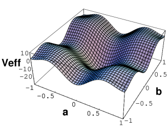
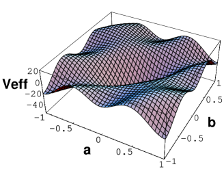
(a)                                                             (b)

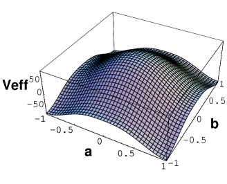
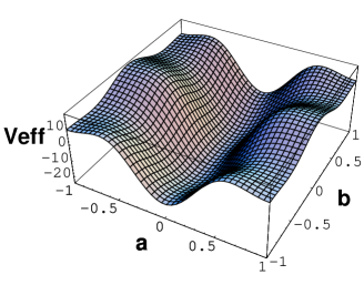
(c)                                                             (d)

Figure 2: The effective potential $V_{\rm eff}(a,b)$ in the $U(3)\times U(3)$ gauge theory on $M^{4}\times(T^{2}/Z_{2})$ with $R_{1}=R_{2}$. (a) In pure gauge theory with $\cos\theta=0$. (b) In pure gauge theory with $\cos\theta=0.6$. (c) In the presence of a minimal set of fermions with $\cos\theta=0$. The global minimum is located at $(a,b)=(1,1)$ which corresponds to $U(1)_{EM}\times U(1)_{Z}$ symmetry. (d) In the presence of parity partners of quarks and leptons and one fermion in the adjoint representation with $\cos\theta=0$. The minimum is located at $(a,b)=(0,\pm 0.269)$. The electroweak symmetry breaks down to $U(1)_{EM}$.

In the presence of fermions, the point $(a,b)=(0,0)$ becomes unstable. The global minimum is located at $(a,b)=(1,1)$ for $|\cos\theta|<0.5$ and at $(a,b)=(0,1)$ or $(1,0)$ for $|\cos\theta|>0.5$. In either case the residual symmetry is $U(1)_{EM}\times U(1)_{Z}$. Although the $SU(2)_{L}$ symmetry is partially broken and $W$ bosons acquire masses, $Z$ bosons remain massless. See fig. 2(c).

Models having the electroweak symmetry breaking are obtained by adding heavy fermions. For each quark/lepton multiplet in (7.2)-(7.6), which has $(\eta_{1},\eta_{2})=(1,1)$ in (5.6), we introduce three parity partners with $(\eta_{1},\eta_{2})=(-1,1),(1,-1),(-1,-1)$. Further we add fermions in the adjoint representation with $(\eta_{1},\eta_{2})=(-1,1)$. The total effective potential is, up to a constant,

$$\hskip-28.45274ptV_{\rm eff}(a,b)^{\rm total}=8I(\hbox{${1\over 2}$}a,\hbox{${1\over 2}$}b)+4I(a,b)-N_{Ad}\Big{\{}8I(\hbox{${1\over 2}$}a+\hbox{${1\over 2}$},\hbox{${1\over 2}$}b)+4I(a+\hbox{${1\over 2}$},b)\Big{\}}$$ (7.17)

$$\hskip-14.22636pt-16N_{F}\Big{\{}I(\hbox{${1\over 2}$}a,\hbox{${1\over 2}$}b)+I(\hbox{${1\over 2}$}a+\hbox{${1\over 2}$},\hbox{${1\over 2}$}b)+I(\hbox{${1\over 2}$}a,\hbox{${1\over 2}$}b+\hbox{${1\over 2}$})+I(\hbox{${1\over 2}$}a+\hbox{${1\over 2}$},\hbox{${1\over 2}$}b+\hbox{${1\over 2}$})\Big{\}}~{}.$$ (7.18)

Here $N_{Ad}$ and $N_{F}$ are the numbers of Weyl fermions in the adjoint representation and of generation of quarks and leptons, respectively. Fermions with $(\eta_{1},\eta_{2})\not=(1,1)$ do not have zero modes. For $N_{F}=3$ the spectrum at low energies is the same as in the minimal model.

With $N_{F}=3$, $N_{Ad}=1$ and $R_{1}=R_{2}$ in (7.18), the global minima of $V_{\rm eff}(a,b)^{\rm total}$ are located at $(a,b)=(0,\pm 0.269)$ for $\cos\theta=0$ and at at $(a,b)=(\pm 0.013,\pm 0.224)$ for $\cos\theta=0.1$. For $\cos\theta>0.133$ the global minimum is located at $(a,b)=(0,0)$. The electroweak symmetry is dynamically broken for $|\cos\theta|<0.133$.

8.  $m_{W}$, $m_{H}$ and $M_{KK}$

One of the most intriguing features in the dynamical gauge-Higgs unification is that the mass of the Higgs boson, $m_{H}$, and the energy scale of the Kaluza-Klein excitations, $M_{KK}$, are predicted in terms of the W boson mass, $m_{W}$. Wilson line phases play the role of Higgs fields in four dimensions. $m_{W}$ is determined from the Wilson line phases and the size of extra dimensions, whereas $m_{H}$ is determined from the effective potential for the Wilson line phases.[18]

The W boson mass arises from the $\,{\rm tr}\,F_{\mu y_{j}}F^{\mu y_{j}}$ term in the Lagrangian. Non-vanishing $(a,b)$ gives

$$m_{W}^{2}=\frac{1}{4\sin^{2}\theta}\left(\frac{a^{2}}{R_{1}^{2}}+\frac{b^{2}}{R_{2}^{2}}-\frac{2ab\cos\theta}{R_{1}R_{2}}\right)~{}.$$ (8.1)

In the model described in (7.18) with $N_{F}=3$, $N_{Ad}=1$ and $R_{1}=R_{2}=R$, one finds that

$$m_{W}=\cases{{\displaystyle 0.135\over\displaystyle R}&for $\cos\theta=0$,\cr{\displaystyle 0.112\over\displaystyle R}&for $\cos\theta=0.1$.\cr}$$ (8.2)

On $M^{4}\times(T^{2}/Z_{2})$ there appear two Higgs doublets in four dimensions. Three of the eight degrees of freedom are absorbed by $W$ and $Z$ bosons. A charged Higgs particle acquires a mass $\sim m_{W}$, while a neutral CP-odd Higgs particle acquires a mass $\sim 2m_{W}$. The most problematic is the mass of two neutral CP-even Higgs particles, which correspond to quantum fluctuations in the directions of the Wilson line phases. By making use of (7.8) and (7.10), the masses are evaluated from the two eigenvalues of the matrix $K^{jk}=g^{2}R^{2}(\partial^{2}V_{\rm eff}/\partial a_{j}\partial a_{k})|_{\rm min}$ where $(a_{1},a_{2})=(a,b)$. They are given by

$$m_{H}=\left\{\matrix{(0.871,3.26)\cr(0.799,4.01)}\right\}\times\bigg{(}{\displaystyle g_{4}^{2}\over\displaystyle 4\pi}\bigg{)}^{1/2}~{}m_{W}\qquad{\rm for~{}}\cos\theta=\cases{0\cr 0.1\cr}$$ (8.3)

where the four-dimensional gauge coupling constant is related to the six-dimensional one by $g_{4}^{2}=g^{2}/(2\pi^{2}R^{2}\sin\theta)$.

(8.2) and (8.3) show how $M_{KK}=1/R$ and $m_{H}$ are related to $m_{W}$ in this scheme. From (8.2) $M_{KK}$ turns out $(7\sim 9)m_{W}$, being too low from the viewpoint of the observational limit. As inferred from (8.1), $m_{W}$ is given, generically in flat space, by

$$M_{KK}\sim 2~{}{\displaystyle\pi\over\displaystyle\theta_{W}}~{}m_{W}~{}~{}.$$ (8.4)

As the minimum of the effective potential for the Wilson line phase $\theta_{W}$ is located typically at $\theta_{W}=(0.2\sim 0.4)\pi$, $M_{KK}$ appears in the range $400\sim 800\,$GeV. Further, it follows from (8.3) that the mass of the lightest Higgs particle is about 10 GeV, which contradicts with the observation. In general one finds, in flat space,

$$m_{H}\sim 0.2~{}\sqrt{\alpha_{w}}~{}{\displaystyle\pi\over\displaystyle\theta_{W}}~{}m_{W}~{}~{},$$ (8.5)

where $\alpha_{w}={g_{4}^{2}}/{4\pi}$. As the Higgs mass is generated by radiative corrections, there appears the factor $\sqrt{\alpha_{w}}$ which leads to a small Higgs mass.

9.  Prospect

We have shown that the dynamical gauge-Higgs unification is achieved in higher dimensional gauge theory. Higgs fields are identified with Wilson line phases in gauge theory. Dynamical symmetry breaking is induced by the Hosotani mechanism.

In the dynamical gauge-Higgs unification $M_{KK}$ and $m_{H}$ are related to $m_{W}$ and $\theta_{W}$. The results (8.4) and (8.5) generically follow when the extra-dimensional space is flat. With a typical value $\theta_{W}=(0.2\sim 0.4)\pi$, both $M_{KK}$ and $m_{H}$ turn out too low.

How can we circumvent this difficulty? One way is to have a model in which the global minimum of the effective potential is located at very small $\theta_{W}$. This goal is, in principle, achieved by tuning the matter content. However, it usually requires to incorporate many additional fields so that the resultant theory is not realistic.

More promising is to consider a gauge theory in higher dimensions where the extra-dimensional space is curved. Gauge theory defined in the Randall-Sundrum warped spacetime is particularly interesting.[21]-[25] It has been recently shown [25] that dynamical gauge-Higgs unification in the Randall-Sundrum warped spacetime leads to, in place of (8.4) and (8.5),

$$\hskip-28.45274ptM_{KK}\sim\sqrt{2\pi kR}~{}{\displaystyle\pi\over\displaystyle\theta_{W}}~{}m_{W}~{}~{},$$ (9.1)

$$\hskip-28.45274ptm_{H}\sim 0.3~{}kR~{}\sqrt{\alpha_{w}}~{}{\displaystyle\pi\over\displaystyle\theta_{W}}~{}m_{W}~{}~{}.$$ (9.2)

Here $k^{2}$ and $R$ are the curvature and size of the extra-dimensional space. If the structure of spacetime is determined at the Planck mass scale, then $k=O(M_{Pl})$. To have $m_{W}\sim 80\,$GeV, the relation $k=O(M_{Pl})$ in turn leads to $kR=12\pm 1$. $kR$ is not a free parameter in the dynamical gauge-Higgs unification scheme. With a typical value $\theta_{W}=(0.2\sim 0.4)\pi$, it is predicted that $M_{KK}=(1.7\sim 3.5)\,$TeV and $m_{H}=(140\sim 280)\,$GeV.

It is very exciting that the mass of the Higgs particle is predicted in the region where the experiments at LHC can certainly explore. Detailed analysis of the interactions of the Higgs particles in the dynamical gauge-Higgs unification scheme will shed light on what to explore in the LHC experiments. We might be able to observe the dynamical gauge symmetry breaking by the Wilson line phases.

Acknowledgment

This work was supported in part by Scientific Grants from the Ministry of Education and Science, Grant No. 13135215, Grant No. 15340078, Grant No. 17043007, and Grant No. 17540257.

References

References

[1]
E. Witten, Phys. Rev. Lett. 38 (1977) 121.
[2]
D.B. Fairlie, Phys. Lett. B82 (1979) 97;
J. Phys. G5 (1979) L55.
[3]
P. Forgacs and N. Manton, Comm. Math. Phys. 72 (1980) 15.
N. Manton, Nucl. Phys. B158 (1979) 141;
[4]
Y. Hosotani, Phys. Lett. B126 (1983) 309.
[5]
Y. Hosotani, Ann. Phys. (N.Y.)190 (1989) 233.
[6]
T.R. Morris, JHEP0501 (2005) 002.
[7]
K. Takenaga, Phys. Lett. B425 (1998) 114;
Phys. Rev. D58 (1998) 026004.
[8]
A. Pomarol and M. Quiros, Phys. Lett. B438 (1998) 255.
[10]
I. Antoniadis, K. Benakli and M. Quiros,
New. J. Phys.3 (2001) 20.
[11]
L. Hall and Y. Nomura, Phys. Rev. D64 (2001) 055003;
R. Barbieri, L. Hall and Y. Nomura,
Phys. Rev. D66 (2002) 045025;
A. Hebecker and J. March-Russell,
Nucl. Phys. B625 (2002) 128;
[12]
M. Kubo, C.S. Lim and H. Yamashita,
Mod. Phys. Lett. A17 (2002) 2249.
[13]
N. Haba, M. Harada, Y. Hosotani and Y. Kawamura,
Nucl. Phys. B657 (2003) 169;
Erratum, ibid. B669 (2003) 381.
[14]
Y. Hosotani, in ”Strong Coupling Gauge Theories and Effective Field
Theories”, ed. M. Harada, Y. Kikukawa and K. Yamawaki (World Scientific
2003), p. 234. (hep-ph/0303066).
[15]
G. Burdman and Y. Nomura, Nucl. Phys. B656 (2003) 3;
C. Csaki, C. Grojean and H. Murayama, Phys. Rev. D67 (2003) 085012;
I. Gogoladze, Y. Mimura and S. Nandi,
Phys. Rev. Lett. 91 (2003) 141801;
C.A. Scrucca, M. Serone, L. Silvestrini and A. Wulzer,
JHEP0402 (2004) 49;
[16]
N. Haba, Y. Hosotani and Y. Kawamura,
Prog. Theoret. Phys. 111 (2004) 265.
[17]
Y. Hosotani, S. Noda and K. Takenaga,
Phys. Rev. D69 (2004) 125014.
[18]
Y. Hosotani, S. Noda and K. Takenaga,
Phys. Lett. B607 (2005) 276.
[19]
N. Haba, Y. Hosotani, Y. Kawamura and T. Yamashita,
Phys. Rev. D70 (2004) 015010;
N. Haba, K. Takenaga, and T. Yamashita,
hep-ph/0411250.
[20]
M. Quiros, in
“Boulder 2002, Particle Physics and Cosmology”, pages 549 - 601.
(hep-ph/0302189).
[21]
L. Randall and R. Sundrum, Phys. Rev. Lett. 83 (1999) 3370.
[22]
S. Chang, J. Hisano, H. Nakano, N. Okada and M. Yamaguchi,
Phys. Rev. D62 (2000) 084025;
T. Gherghetta and A. Pomarol,
Nucl. Phys. B586 (2000) 141.
[23]
R. Contino, Y. Nomura and A. Pomarol, Nucl. Phys. B671 (2003) 148;
K. Agashe, R. Contino and A. Pomarol, hep-ph/0412089.
[24]
K. Oda and A. Weiler, Phys. Lett. B606 (2005) 408.
[25]
Y. Hosotani and M. Mabe, hep-ph/0503020 (to appear in Phys. Lett. B).