The effects of non-standard Z couplings on the lepton polarizations in Bsโ†’ฮณโ€‹โ„“+โ€‹โ„“โˆ’โ†’subscript๐ต๐‘ ๐›พsuperscriptโ„“superscriptโ„“B_{s}\rightarrow\gamma\,\ell^{+}\ell^{-} decays

Gรผrsevil Turan
Physics Department, Middle East Technical University

06531 Ankara, Turkey

The fact that the measured $B\rightarrow\pi\,\pi\,,\,\pi\,K$ branching ratios exhibit puzzling patterns has received a lot of attention in the literature and motivated the formulation of a series of new physics scenarios with enhanced Z-penguins. In this work, we analyze the effect of such an enhancement on the lepton polarization asymmetries of Bsโ†’ฮณโ€‹โ„“+โ€‹โ„“โˆ’โ†’subscript๐ต๐‘ ๐›พsuperscriptโ„“superscriptโ„“B_{s}\rightarrow\gamma\ell^{+}\ell^{-} decays by applying the results of a specific scenario for the solution of โ€œBโ†’ฯ€โ€‹Kโ†’๐ต๐œ‹๐พB\to\pi K puzzleโ€.

In the Standard Model (SM), CP violation originates from the the Cabibboโ€“Kobayashiโ€“Maskawa (CKM) three generation quark mixing matrix [1], and this picture successfully explains the observed CP violation in the Kaon sector . As for the B-sector, in the near future, more number of experimental tests will be possible at the the B-factories providing stringent testing of the SM mechanism of CP violation. In the mean time, some of the current $B$-factory data seems to be at variance with the SM description of CP violation for a number of processes. These processes can be grouped into two systems: $B\rightarrow\pi\pi$ , $B\rightarrow\pi K$ and $B\rightarrow\psi K$ , $B\rightarrow\phi K$ and have received a lot of attention in the literature. In particular;

  • โ€ข

    The BaBar and Belle collaborations have recently reported the branching ratios of $B_{d}\to\pi^{0}\pi^{0}$ decays [2, 3], which turn out to be as large as six times the value given in a recent calculation [4] within QCD factorization [5], whereas the calculation of $B_{d}\to\pi^{+}\pi^{-}$ gives a branching ratio about two times larger than the current experimental average. On the other hand, the calculation of $B^{+}\to\pi^{+}\pi^{0}$ agrees with the data quite well. As was recently pointed out [6], this โ€Bโ†’ฯ€โ€‹ฯ€โ†’๐ต๐œ‹๐œ‹B\rightarrow\pi\pi hierarchyโ€ can be conveniently accommodated in the SM through non-factorizable hadronic interference effects.

    The CLEO, BaBar and Belle collaborations have also measured the ratios of charged $R_{\rm c}$ and neutral $R_{\rm n}$ branching ratios for $B\rightarrow\pi K$ [7] that are affected significantly by colour-allowed electroweak (EW) penguins, and reported a pattern of $R_{\rm c}>1$ and $R_{\rm n}<1$. As noted in [8], this pattern contradicts with the one obtained for decays $B\rightarrow\pi K$ as the extension of the results for $B\rightarrow\pi\pi$ decays using SU(3) symmetry. It has been pointed out that the quantities that may only get contributions from colour-suppressed forms do not show any anomalous behavior like $R_{\rm c}$ and $R_{\rm n}$ do, so that this โ€œBโ†’ฯ€โ€‹Kโ†’๐ต๐œ‹๐พB\to\pi K puzzleโ€ may be a manifestation of new physics (NP) in the EW penguin sector [6, 8, 9].

  • โ€ข

    The decay $B_{d}\to\phi K_{\rm s}$ provides another suggestive contrast with the SM expectation. There is a very good agreement between the SM value of sinโก2โ€‹ฮฒฯ•โ€‹Ks2subscript๐›ฝitalic-ฯ•subscript๐พ๐‘ \sin 2\beta_{\phi K_{s}}, which is the most precise information on CP violation in the quark sector, and the most well established B-factory result determined from the decay Bโ†’ฯˆโ€‹Ksโ†’๐ต๐œ“subscript๐พ๐‘ B\rightarrow\psi K_{s}. However, for the decay Bโ†’ฯ•โ€‹Ksโ†’๐ตitalic-ฯ•subscript๐พ๐‘ B\rightarrow\phi K_{s}, whose time dependent CP violation is predicted to be the same as in Bโ†’ฯˆโ€‹Ksโ†’๐ต๐œ“subscript๐พ๐‘ B\rightarrow\psi K_{s} by the SM, experimental results seem to be providing a contrast between sinโก2โ€‹ฮฒฯˆโ€‹Ks2subscript๐›ฝ๐œ“subscript๐พ๐‘ \sin 2\beta_{\psi K_{s}} and sinโก2โ€‹ฮฒฯ•โ€‹Ks2subscript๐›ฝitalic-ฯ•subscript๐พ๐‘ \sin 2\beta_{\phi K_{s}}. Since within the SM, this transition is governed by QCD penguins [10] and receives sizeable EW penguin contributions [11, 12], with more data, this would suggest definite evidence for NP beyond the SM.

It has been argued that a promising class of models that can explain the discrepancies summarized above involve flavor changing couplings of the Z-boson to bยฏโ€‹sยฏ๐‘๐‘ \bar{b}s. The possibility of NP with the dominant $Z^{0}$-penguin contributions was first considered in [13]โ€“[15], where correlations between rare $K$ decays and $\varepsilon^{\prime}/\varepsilon$ were studied in model-independent analyses and also within particular supersymmetric scenarios. It was generalized to rare $B$ decays in [16]. Recently, in [17], the effects of enhanced Z penguins on the lepton polarization asymmetries of bโ†’sโ€‹โ„“+โ€‹โ„“โˆ’โ†’๐‘๐‘ superscriptโ„“superscriptโ„“b\rightarrow s\ell^{+}\ell^{-} have been considered.

In this work we analyze the effects of such a non-standard Z coupling on the lepton polarization asymmetries of Bsโ†’ฮณโ€‹โ„“+โ€‹โ„“โˆ’โ†’subscript๐ต๐‘ ๐›พsuperscriptโ„“superscriptโ„“B_{s}\rightarrow\gamma\ell^{+}\ell^{-} decays by applying the results of a specific scenario considered in [6] for the solution of โ€œBโ†’ฯ€โ€‹Kโ†’๐ต๐œ‹๐พB\to\pi K puzzleโ€. This basically involves considering the decays $B\rightarrow\pi\pi$ and $B\rightarrow\pi K$ simultaneously within the SM and its simplest extension in which NP enters dominantly through enhanced EW penguins with new weak phases. Since $B\rightarrow\pi\pi$ decays are only insignificantly effected by EW penguins, this system can be described as in the SM and allows the extraction of the relevant hadronic parameters by assuming only the isospin symmetry. Using SU(3) flavor symmetry it is then determined the hadronic $B\rightarrow\pi K$ parameters through their $B\rightarrow\pi\pi$ counterparts. Here there are two parameters, $C(x_{t})$ with $x_{t}=m^{2}_{t}/M^{2}_{W}$, which is the Z- penguin function and $\theta$, its complex phase. The relevant EW penguin parameters for $B\rightarrow\pi K$ decays are $q$ and $\phi$, whose SM values are $q=0.69$ and $\phi=0$. It has been found that pattern of $R_{c}>1$ and $R_{n}<1$ can not be described properly for these SM values; however, treating them as free parameters and using the hadronic $B\rightarrow\pi K$ parameters, it is possible to convert the experimental results for $R_{c}$ and $R_{n}$ into the values of $q$ and $\phi$,

$$q=1.78^{+1.24}_{-0.97}\,\,,\,\,\phi=-(85^{+11}_{-13})^{\circ}\,\,,$$ (1)

which describe all currently available data.

For the radiative Bsโ†’ฮณโ€‹โ„“+โ€‹โ„“โˆ’โ†’subscript๐ต๐‘ ๐›พsuperscriptโ„“superscriptโ„“B_{s}\rightarrow\gamma\,\ell^{+}\ell^{-}decay, the basic quark level process is bโ†’sโ€‹โ„“+โ€‹โ„“โˆ’โ†’๐‘๐‘ superscriptโ„“superscriptโ„“b\rightarrow s\ell^{+}\ell^{-}, which can be written as

$\displaystyle{\cal H}_{eff}$ $\displaystyle=$ ฮฑโ€‹GF2โ€‹ฯ€โ€‹Vtโ€‹bโ€‹Vtโ€‹sโˆ—โ€‹{C9eโ€‹fโ€‹fโ€‹(sยฏโ€‹ฮณฮผโ€‹PLโ€‹b)โ€‹โ„“ยฏโ€‹ฮณฮผโ€‹โ„“+C10โ€‹(sยฏโ€‹ฮณฮผโ€‹PLโ€‹b)โ€‹โ„“ยฏโ€‹ฮณฮผโ€‹ฮณ5โ€‹โ„“โˆ’2โ€‹C7โ€‹mbq2โ€‹(sยฏโ€‹iโ€‹ฯƒฮผโ€‹ฮฝโ€‹qฮฝโ€‹PRโ€‹b)โ€‹โ„“ยฏโ€‹ฮณฮผโ€‹โ„“},๐›ผsubscript๐บ๐น2๐œ‹subscript๐‘‰๐‘ก๐‘superscriptsubscript๐‘‰๐‘ก๐‘ superscriptsubscript๐ถ9๐‘’๐‘“๐‘“ยฏ๐‘ subscript๐›พ๐œ‡subscript๐‘ƒ๐ฟ๐‘ยฏโ„“superscript๐›พ๐œ‡โ„“subscript๐ถ10ยฏ๐‘ subscript๐›พ๐œ‡subscript๐‘ƒ๐ฟ๐‘ยฏโ„“superscript๐›พ๐œ‡subscript๐›พ5โ„“2subscript๐ถ7subscript๐‘š๐‘superscript๐‘ž2ยฏ๐‘ ๐‘–subscript๐œŽ๐œ‡๐œˆsuperscript๐‘ž๐œˆsubscript๐‘ƒ๐‘…๐‘ยฏโ„“superscript๐›พ๐œ‡โ„“\displaystyle\frac{\alpha G_{F}}{\sqrt{2}\,\pi}V_{tb}V_{ts}^{*}\Bigg{\{}C_{9}^{eff}(\bar{s}\gamma_{\mu}P_{L}b)\,\bar{\ell}\gamma^{\mu}\ell+C_{10}(\bar{s}\gamma_{\mu}P_{L}b)\,\bar{\ell}\gamma^{\mu}\gamma_{5}\ell-2C_{7}\frac{m_{b}}{q^{2}}(\bar{s}i\sigma_{\mu\nu}q^{\nu}P_{R}b)\bar{\ell}\gamma^{\mu}\ell\Bigg{\}}~{},

where $P_{L,R}=(1\mp\gamma_{5})/2$ , $q$ is the momentum transfer and $V_{ij}$โ€™s are the corresponding elements of the CKM matrix. The values of the individual Wilson coefficients that appear in the SM are listed in Table (1).

$C_{1}$ $C_{2}$ $C_{3}$ $C_{4}$ $C_{5}$ $C_{6}$ $C_{7}^{\rm eff}$ $C_{9}$ $C_{10}$
$-0.248$ $+1.107$ $+0.011$ $-0.026$ $+0.007$ $-0.031$ $-0.313$ $+4.344$ $-4.624$
Table 1: Values of the SM Wilson coefficients at $\mu\sim m_{b}$ scale.

As for the $C_{9}$, its value is given as [18, 19]

$\displaystyle C_{9}^{eff}(\mu)=C_{9}(\mu)+Y(\mu)\,\,,$ (3)

where the function $Y(\mu)$ contains a part which arises from the one loop contributions of the four quark operators $O_{1}$,โ€ฆ,$O_{6}$ whose explicit forms can be found in [18, 20], and also a part which estimates the long-distance contributions from intermediate states J/ฯˆ,ฯˆโ€ฒ,โ€ฆโ€‹[19, 21]๐ฝ๐œ“superscript๐œ“โ€ฒโ€ฆ[19, 21]J/\psi,\psi^{\prime},...\cite[cite]{[\@@bibref{}{LD,KS}{}{}]}.

In the SM, the Wilson coefficient $C_{10}$ is given by

$\displaystyle C_{10}$ $\displaystyle=$ $\displaystyle\frac{-1}{\sin^{2}\theta_{w}}\,Y\,,$ (4)

with

$\displaystyle Y$ $\displaystyle=$ $\displaystyle C(x_{t})-B(x_{t})\,,$ (5)

where explicit formulae of $C(x_{t})$ and $B(x_{t})$ can be found in [20, 22]. For the rare B decays with $\ell^{+}\ell^{-}$ in the final state the short distance function $Y$ can be parametrized as

$\displaystyle Y$ $\displaystyle=$ $\displaystyle|C|\,e^{i\theta}+0.18\,,$ (6)

and the connection between the rare decays and the $B\rightarrow\pi K$ system is established by relating the parameters $(C,\theta)$ to the EW penguin parameters $(q,\phi)$ by means of a renormalization group analysis that yields [6]

$\displaystyle|C|\,e^{i\theta}=2.35\bar{q}e^{i\phi}-0.82\,\,,\,\,\bar{q}=q\Bigg{[}\frac{|V_{ub}/V_{cb}|}{0.086}\Bigg{]}.$ (7)

Furthermore, $Y$ is rewritten as

$\displaystyle Y$ $\displaystyle=$ $\displaystyle|Y|\,e^{i\theta_{Y}}\,,$ (8)

where the constraint that $|Y|\leq 2.2$ follows from the BaBar and Belle data on Bโ†’Xsโ€‹ฮผ+โ€‹ฮผโˆ’โ†’๐ตsubscript๐‘‹๐‘ superscript๐œ‡superscript๐œ‡B\rightarrow X_{s}\mu^{+}\mu^{-} decay [23]. The central value for $Y$ resulting from (1) violates the upper bound of $|Y|$, however considering only the subset of those values of $(q,\phi)$ that satisfies $|Y|=2.2$ gives $\theta_{Y}=-(103\pm 12)^{\circ}$. Now, with the contributions from the enhanced and complex value of the bโ€‹sโ€‹Z๐‘๐‘ ๐‘bsZ vertex, $C_{10}$ becomes

$\displaystyle C_{10}$ $\displaystyle=$ $\displaystyle\frac{-2.2}{\sin^{2}\theta_{w}}\,e^{i(103/180)\pi}\,,$ (9)

and has a magnitude twice the SM one.

Having established the general form of the effective Hamiltonian, the next step is to calculate the matrix element of the Bsโ†’ฮณโ€‹โ„“+โ€‹โ„“โˆ’โ†’subscript๐ต๐‘ ๐›พsuperscriptโ„“superscriptโ„“B_{s}\rightarrow\gamma\,\ell^{+}\ell^{-} decay, which is induced by the inclusive bโ†’sโ€‹ฮณโ€‹โ„“+โ€‹โ„“โˆ’โ†’๐‘๐‘ ๐›พsuperscriptโ„“superscriptโ„“b\rightarrow s\gamma\,\ell^{+}\ell^{-} one. Thus, the related matrix element can be found from the bโ†’sโ€‹โ„“+โ€‹โ„“โˆ’โ†’๐‘๐‘ superscriptโ„“superscriptโ„“b\rightarrow s\,\ell^{+}\ell^{-} decay by attaching a photon line to any charged internal or external line. However, contributions coming from the release of the free photon from any charged internal line will be suppressed by a factor of $m^{2}_{b}/M^{2}_{W}$ and can be neglected. When a photon is released from the initial quark lines it contributes to the so-called โ€structure dependentโ€ (SD) part of the amplitude, whereas, โ€internal Bremsstrahlungโ€ (IB) part of the amplitude arises when a photon is radiated from one of the final $\ell$- leptons. Therefore, the total matrix element can be written as a sum of the SD and the IB contributions:

$${\cal M}={\cal M}_{SD}+{\cal M}_{IB}\,,$$ (10)

with

$\displaystyle{\cal M}_{SD}$ $\displaystyle=$ $\displaystyle\langle\gamma(k)\left|{\cal H}_{eff}\right|B(p_{B})\rangle\,\,,\,\,{\cal M}_{IB}=\langle 0\left|{\cal H}_{eff}\right|B(p_{B})\rangle\,\,.$ (11)

The structures in Eq. (11) are parametrized in terms of the various form factors $f,g,f_{1},g_{1}$, calculated in the framework of light-cone QCD sum rules [24, 25] and in the framework of the light front quark model [26]. In addition, it has been proposed another model in [27] for the $B\rightarrow\gamma$ form factors which obey all the restrictions obtained from the gauge invariance combined with the large energy effective theory.

By using the explicit expressions of the parametrizations for the above matrix elements in terms of the form factors, which can be found in [25], we calculate dilepton mass distribution for $B\rightarrow\gamma\,\ell^{-}\ell^{+}$ decay as [28, 29]

dโ€‹ฮ“dโ€‹s=ฮฑ3โ€‹GF2โ€‹|Vtโ€‹bโ€‹Vtโ€‹sโˆ—|2210โ€‹ฯ€4โ€‹mBโ€‹ฮ”,๐‘‘ฮ“๐‘‘๐‘ superscript๐›ผ3subscriptsuperscript๐บ2๐นsuperscriptsubscript๐‘‰๐‘ก๐‘subscriptsuperscript๐‘‰โˆ—๐‘ก๐‘ 2superscript210superscript๐œ‹4subscript๐‘š๐ตฮ”\displaystyle\frac{d\Gamma}{ds}=\frac{\alpha^{3}\,G^{2}_{F}\,|V_{tb}V^{\ast}_{ts}|^{2}}{2^{10}\pi^{4}}\,m_{B}\Delta~{}, (12)

where

$\displaystyle\Delta$ $\displaystyle=$ $\displaystyle\Bigg{\{}(1-s)^{3}v\,\Bigg{(}\,4m_{B}^{2}r\,\mbox{\rm Re}[A_{1}B_{1}^{\ast}+A_{2}B_{2}^{\ast}]+\,\frac{2}{3}m_{B}^{2}\Big{(}\left|A_{1}\right|^{2}+\left|A_{2}\right|^{2}+\left|B_{1}\right|^{2}$ (13)
$\displaystyle+$ $\displaystyle\left|B_{2}\right|^{2}\Big{)}(s-r)\Bigg{)}+4f_{B}\,m_{\ell}\,{\rm ln}[u]\,\mbox{\rm Re}[(A_{1}+B_{1})F^{\ast}]\,(1-s)^{2}$
$\displaystyle-$ $\displaystyle 4f_{B}^{2}\,\left|F\right|^{2}\Bigg{(}2v\frac{s}{(1-s)}+\,{\rm ln}[u]\Bigg{[}2+\frac{2(2r-1)}{(1-s)}-(1-s)\Bigg{]}\Bigg{)}\Bigg{\}}~{}.$

Now, we would like to discuss the lepton polarizations in the rare Bsโ†’ฮณโ€‹โ„“+โ€‹โ„“โˆ’โ†’subscript๐ต๐‘ ๐›พsuperscriptโ„“superscriptโ„“B_{s}\rightarrow\gamma\,\ell^{+}\ell^{-}decays. For this, it is introduced spin projection operator $N=(1+\gamma_{5}\not\!S_{i})/2$ for $\ell^{-}$, where $i=L,~{}T,~{}N$ correspond to longitudinal, transverse and normal polarizations, respectively. In the rest frame of $\ell^{-}$, the orthogonal unit vectors $S_{i}$ are defined as

$\displaystyle S^{\mu}_{L}$ $\displaystyle\equiv$ $\displaystyle(0,\vec{e}_{L})=\Bigg{(}0,\frac{\vec{p}_{1}}{|\vec{p}_{1}|}\Bigg{)}\,,$
$\displaystyle S^{\mu}_{N}$ $\displaystyle\equiv$ $\displaystyle(0,\vec{e}_{N})=\Bigg{(}0,\frac{\vec{k}\times\vec{p}_{1}}{|\vec{k}\times\vec{p}_{1}|}\Bigg{)}\,,$
$\displaystyle S^{\mu}_{T}$ $\displaystyle\equiv$ $\displaystyle(0,\vec{e}_{T})=\Bigg{(}0,\vec{e}_{N}\times\vec{e}_{L}\Bigg{)}\,.$ (14)

The longitudinal unit vector $S_{L}$ is boosted to the CM frame of $\ell^{+}\ell^{-}$ by Lorentz transformation:

$\displaystyle S^{\mu}_{L,CM}$ $\displaystyle=$ $\displaystyle\Bigg{(}\frac{|\vec{p}_{1}|}{m_{\ell}},\frac{E_{\ell}~{}\vec{p}_{1}}{m_{\ell}|\vec{p}_{1}|}\Bigg{)}\,,$ (15)

while $P_{T}$ and $P_{N}$ are not changed by the boost since they lie in the perpendicular directions. For $i=L,~{}T,~{}N$, the polarization asymmetries $P_{i}$ of the final $\ell^{-}$ lepton are defined as

Piโ€‹(s)subscript๐‘ƒ๐‘–๐‘ \displaystyle P_{i}(s) $\displaystyle=$ dโ€‹ฮ“dโ€‹sโ€‹(nโ†’=eโ†’i)โˆ’dโ€‹ฮ“dโ€‹sโ€‹(nโ†’=โˆ’eโ†’i)dโ€‹ฮ“dโ€‹sโ€‹(nโ†’=eโ†’i)+dโ€‹ฮ“dโ€‹sโ€‹(nโ†’=โˆ’eโ†’i).๐‘‘ฮ“๐‘‘๐‘ โ†’๐‘›subscriptโ†’๐‘’๐‘–๐‘‘ฮ“๐‘‘๐‘ โ†’๐‘›subscriptโ†’๐‘’๐‘–๐‘‘ฮ“๐‘‘๐‘ โ†’๐‘›subscriptโ†’๐‘’๐‘–๐‘‘ฮ“๐‘‘๐‘ โ†’๐‘›subscriptโ†’๐‘’๐‘–\displaystyle\frac{\frac{d\Gamma}{ds}(\vec{n}=\vec{e}_{i})-\frac{d\Gamma}{ds}(\vec{n}=-\vec{e}_{i})}{\frac{d\Gamma}{ds}(\vec{n}=\vec{e}_{i})+\frac{d\Gamma}{ds}(\vec{n}=-\vec{e}_{i})}\,. (16)

After some algebra, we obtain the following expressions for the differential polarization components of the $\ell^{-}$ lepton in Bsโ†’ฮณโ€‹โ„“+โ€‹โ„“โˆ’โ†’subscript๐ต๐‘ ๐›พsuperscriptโ„“superscriptโ„“B_{s}\rightarrow\gamma\,\ell^{+}\ell^{-}decays:

PLโ€‹(s)subscript๐‘ƒ๐ฟ๐‘ \displaystyle P_{L}(s) $\displaystyle=$ $\displaystyle\frac{1}{6v\Delta}\Bigg{\{}4m^{2}_{B}v^{3}s(1-s)^{3}(\left|A_{1}\right|^{2}+\left|A_{2}\right|^{2}-\left|B_{1}\right|^{2}-\left|B_{2}\right|^{2})$ (17)
$\displaystyle+$ $\displaystyle 24f_{B}m_{\ell}(s-1)\Bigg{[}(s-1)\mbox{\rm Re}[(A_{1}-B_{1})F^{\ast}]\Big{(}v+\frac{(2r-s)}{s}{\rm ln}[u]\Big{)}$
$\displaystyle+$ $\displaystyle(1+s)\mbox{\rm Re}[(A_{2}+B_{2})F^{\ast}]\Big{(}v(1-s)-\frac{2r}{s}{\rm ln}[u]\Big{)}\Bigg{]}\Bigg{\}}\,,$
PTโ€‹(s)subscript๐‘ƒ๐‘‡๐‘ \displaystyle P_{T}(s) $\displaystyle=$ $\displaystyle\frac{1}{\Delta}\Bigg{\{}\frac{(2\sqrt{r}-\sqrt{s})}{sv}(1-s)f_{B}m_{B}\pi\Bigg{(}\pm sv^{2}(1+s)\mbox{\rm Re}[(A_{1}-B_{1})F^{\ast}]$ (18)
$\displaystyle+$ $\displaystyle(s-1)(4r+s)\mbox{\rm Re}[(A_{2}+B_{2})F^{\ast}]\Bigg{)}$
$\displaystyle-$ $\displaystyle\frac{\pi v}{4\sqrt{s}}(s-1)^{2}2m_{B}^{2}\sqrt{r}(s-1)s\,\mbox{\rm Re}[(A_{1}+B_{1})(A_{2}+B_{2})^{\ast}]\Bigg{\}}\,,$
PNโ€‹(s)subscript๐‘ƒ๐‘๐‘ \displaystyle P_{N}(s) $\displaystyle=$ $\displaystyle\frac{\pi}{4\Delta}(1-s)m_{B}\Bigg{\{}2m_{B}(1-s)^{2}\sqrt{rs}\,v^{2}(\mbox{\rm Im}[A_{1}B_{2}^{\ast}]+\mbox{\rm Im}[A_{2}B_{1}^{\ast}])$
$\displaystyle-$ $\displaystyle 4(2\sqrt{r}-\sqrt{s})f_{B}\Big{(}(1+s)\mbox{\rm Im}[(A_{1}+B_{1})F^{\ast}]+(1-s)\mbox{\rm Im}[(A_{2}-B_{2})F^{\ast}]\Big{)}\Bigg{\}}\,.$

We present now our numerical analysis about the differential polarization asymmetries PLโ€‹(s)subscript๐‘ƒ๐ฟ๐‘ P_{L}(s), PTโ€‹(s)subscript๐‘ƒ๐‘‡๐‘ P_{T}(s) and PNโ€‹(s)subscript๐‘ƒ๐‘๐‘ P_{N}(s) of $\ell^{-}$ for the Bsโ†’ฮณโ€‹โ„“+โ€‹โ„“โˆ’โ†’subscript๐ต๐‘ ๐›พsuperscriptโ„“superscriptโ„“B_{s}\rightarrow\gamma\ell^{+}\ell^{-} decays with $\ell=\mu,\tau$, as well as the averaged polarization asymmetries $<P_{L}>$, $<P_{T}>$ and $<P_{N}>$. The input parameters used in our numerical analysis are as follows:

$\displaystyle m_{B}=5.28\,GeV\,,\,m_{b}=4.8\,GeV\,,\,m_{\mu}=0.105\,GeV\,,\,m_{\tau}=1.78\,GeV\,,$
fB=0.2โ€‹Gโ€‹eโ€‹V,|Vtโ€‹bโ€‹Vtโ€‹sโˆ—|=0.045,ฮฑโˆ’1=137,GF=1.17ร—10โˆ’5โ€‹Gโ€‹eโ€‹Vโˆ’2formulae-sequencesubscript๐‘“๐ต0.2๐บ๐‘’๐‘‰formulae-sequencesubscript๐‘‰๐‘ก๐‘subscriptsuperscript๐‘‰๐‘ก๐‘ 0.045formulae-sequencesuperscript๐›ผ1137subscript๐บ๐น1.17superscript105๐บ๐‘’superscript๐‘‰2\displaystyle f_{B}=0.2\,GeV\,,\,\,|V_{tb}V^{*}_{ts}|=0.045\,\,,\,\,\alpha^{-1}=137\,\,,G_{F}=1.17\times 10^{-5}\,GeV^{-2}
ฯ„Bs=1.54ร—10โˆ’12โ€‹s.subscript๐œsubscript๐ต๐‘ 1.54superscript1012๐‘ \displaystyle\tau_{B_{s}}=1.54\times 10^{-12}\,s\,. (20)

To make some numerical predictions, we also need the explicit forms of the form factors $g,~{}f,~{}g_{1}$ and $f_{1}$. In this work we have used the values calculated in the framework of light-cone QCD sum rules given in [25].

We also like to note a technical point about calculations of averaged polarization asymmetries. The averaging procedure which we have adopted is

โŸจPiโŸฉ=โˆซ(2โ€‹mโ„“/mB)21โˆ’ฮดPiโ€‹(s)โ€‹dโ€‹ฮ“dโ€‹sโ€‹๐‘‘sโˆซ(2โ€‹mโ„“/mB)21โˆ’ฮดdโ€‹ฮ“dโ€‹sโ€‹๐‘‘s.delimited-โŸจโŸฉsubscript๐‘ƒ๐‘–subscriptsuperscript1๐›ฟsuperscript2subscript๐‘šโ„“subscript๐‘š๐ต2subscript๐‘ƒ๐‘–๐‘ ๐‘‘ฮ“๐‘‘๐‘ differential-d๐‘ subscriptsuperscript1๐›ฟsuperscript2subscript๐‘šโ„“subscript๐‘š๐ต2๐‘‘ฮ“๐‘‘๐‘ differential-d๐‘ \langle P_{i}\rangle=\frac{\int^{1-\delta}_{(2m_{\ell}/m_{B})^{2}}\,P_{i}(s)\,\frac{d\Gamma}{ds}ds}{\int^{1-\delta}_{(2m_{\ell}/m_{B})^{2}}\,\frac{d\Gamma}{ds}ds}\,. (21)

We note that the part of dโ€‹ฮ“/dโ€‹s๐‘‘ฮ“๐‘‘๐‘ d\Gamma/ds in (12) which receives contribution from the $\left|{\cal M}_{IB}\right|^{2}$ term has infrared singularity due to the emission of soft photon. To obtain a finite result from these integrations, we follow the approach described in [25] and impose a cut on the photon energy, i.e., we require $E_{\gamma}\geq 25$ MeV, which corresponds to detect only hard photons experimentally. This cut implies that $E_{\gamma}\geq\delta\,m_{B}/2$ with $\delta=0.01$.

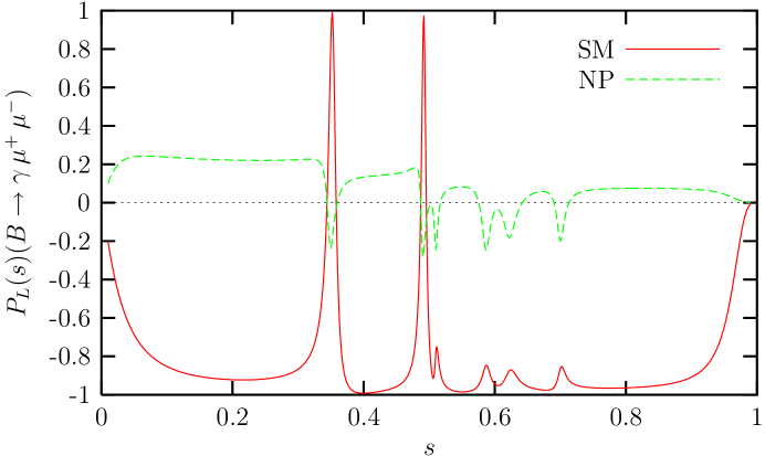
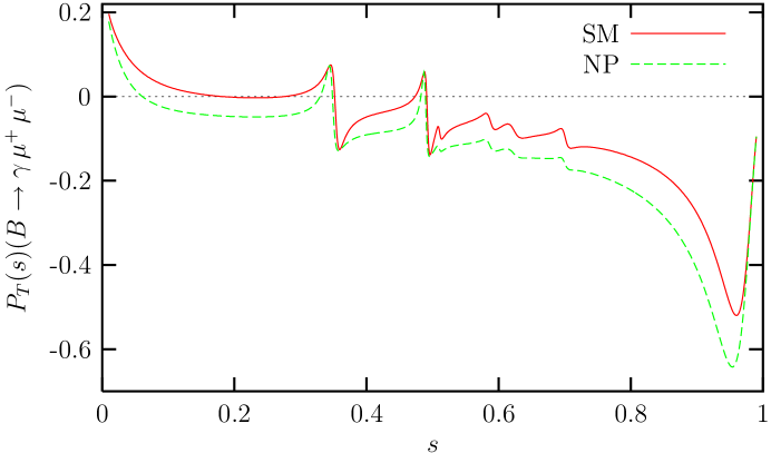
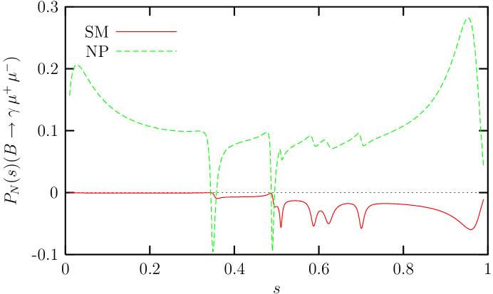
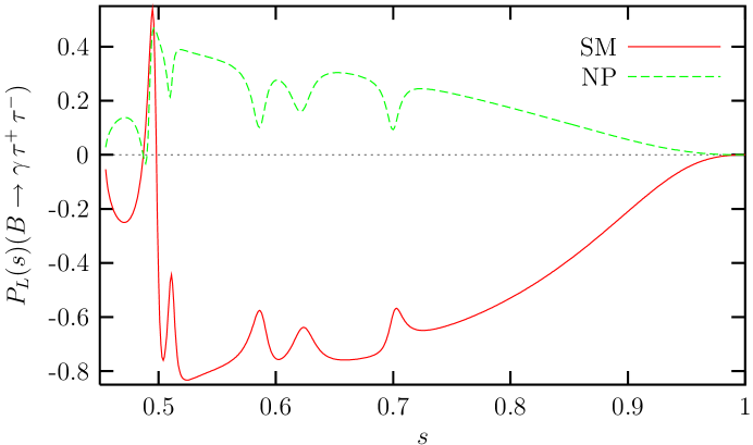
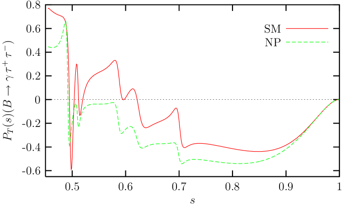
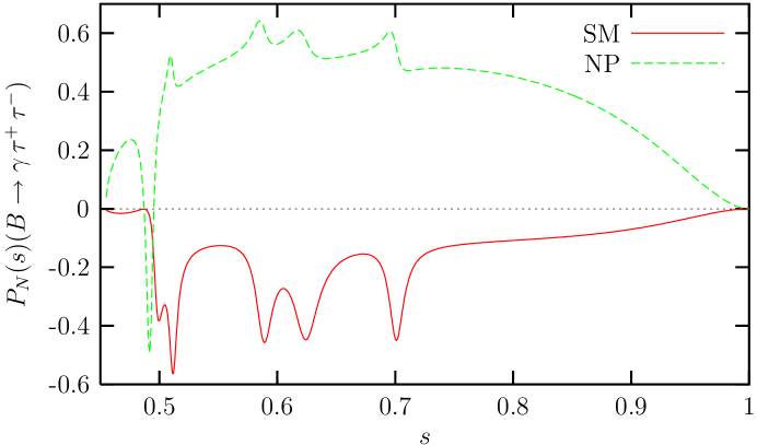
In Figs. (1)-(6) we present our results for the various differential polarization asymmetries within the SM and also with the new value of the coefficient $C_{10}$ given by (9), which results from the enhanced values of the Z penguins. In table (2), we have given the averaged values of these asymmetries. As can be seen, the new value of $C_{10}$ can give substantial changes in the SM results. We note that due to the complex and enhanced value of the bโ€‹sโ€‹Z๐‘๐‘ ๐‘bsZ vertex, the value of longitudinal polarizations decrease as compared to their SM values for both decay modes, however, the transverse and normal asymmetries show a substantial increase from their respective SM values. This increase is especially manifest for $P_{N}$, which changes its sign too as compared to its SM value and its magnitude increases by one order of magnitude for $\mu$ mode, and by almost 200 $\%$ for $\tau$ mode.

Therefore, future measurements of the enhanced normal and transverse polarization asymmetry would be a suitable testing ground for the validity of a complex bโ€‹sโ€‹Z๐‘๐‘ ๐‘bsZ vertex and the model in ref. [6].

Decay Mode Bsโ†’ฮณโ€‹ฮผ+โ€‹ฮผโˆ’โ†’subscript๐ต๐‘ ๐›พsuperscript๐œ‡superscript๐œ‡B_{s}\rightarrow\gamma\,\mu^{+}\mu^{-} Bsโ†’ฮณโ€‹ฯ„+โ€‹ฯ„โˆ’โ†’subscript๐ต๐‘ ๐›พsuperscript๐œsuperscript๐œB_{s}\rightarrow\gamma\,\tau^{+}\tau^{-}
BR $\times 10^{8}$ ${\cal P}^{-}_{L}$ ${\cal P}^{-}_{T}$ ${\cal P}^{-}_{N}$ BR $\times 10^{8}$ ${\cal P}^{-}_{L}$ ${\cal P}^{-}_{T}$ ${\cal P}^{-}_{N}$
SM 1.51 - 0.85 - 0.07 - 0.01 1.14 - 0.23 - 0.19 - 0.07
enhanced bsZ 3.70 0.08 -0.15 0.10 4.68 0.07 -0.25 0.22
Table 2: Predictions of the observables.

References

  • [1] N. Cabibbo, Phys. Rev. Lett.ย 10, (1963) 531; M. Kobayashi and T. Maskawa, Prog.ย Theor.ย Phys.ย 49, (1973) 652.
  • [2] B. Aubert et al.ย  [BaBar Collaboration], Phys. Rev. Lett.ย 91, (2003) 241801.
  • [3] K. Abe et al.ย  [Belle Collaboration], Phys. Rev. Lett.ย 91, (2003) 261801.
  • [4] M. Beneke and M. Neubert, Nucl.ย Phys.ย B675, (2003) 333.
  • [5] M. Beneke, G. Buchalla, M. Neubert and C.T. Sachrajda, Phys.ย Rev.ย Lett.ย 83, (1999) 1914.
  • [6] A.J. Buras, R. Fleischer, S. Recksiegel and F. Schwab, Phys. Rev. Lett. 92, (2004) 101804; A.J. Buras, R. Fleischer, S. Recksiegel and F. Schwab, hep-ph/0402112.
  • [7] A.J. Buras and R. Fleischer, Eur.ย Phys.ย J.ย C11 (1999) 93.
  • [8] A.J. Buras and R. Fleischer, Eur.ย Phys.ย J.ย C16, (2000) 97.
  • [9] A.J. Buras, R. Fleischer, S. Recksiegel and F. Schwab, Eur.ย Phys.ย J.ย C32, (2003) 45.
  • [10] D. London and R. Peccei, Phys.ย Lett.ย B223, (1989) 257;
    N.G. Deshpande and J. Trampetic, Phys.ย Rev.ย D41, (1990) 895 and 2926;
    J.-M. Gรฉrard and W.-S. Hou, Phys.ย Rev.ย D43, (1991) 2909.
  • [11] R. Fleischer, Z.ย Phys.ย C62, (1994) 81.
  • [12] N.G. Deshpande and X.-G. He, Phys.ย Lett.ย B336, (1994) 471.
  • [13] A.J. Buras and L. Silvestrini, Nucl.ย Phys.ย B546, (1999) 299.
  • [14] A.J. Buras, A. Romanino and L. Silvestrini, Nucl.ย Phys.ย B520, (1998) 3.
  • [15] A.J. Buras, G. Colangelo, G. Isidori, A. Romanino and L. Silvestrini, Nucl.ย Phys.ย B566, (2000) 3.
  • [16] G. Buchalla, G. Hiller and G. Isidori, Phys.ย Rev.ย D63, (2001) 014015;
    D. Atwood and G. Hiller, LMU-09-03 [hep-ph/0307251].
  • [17] S. Rai Choudhury and N. Gaur, hep-ph/0402273.
  • [18] B.ย Grinstein, M.ย J.ย Savage and M.ย B.ย Wise, Nucl. Phys. B319, (1989) 271; A.ย J.ย Buras and M.ย Mรผnz, Phys. Rev. D52, (1995) 186.
  • [19] A.ย Ali, T.ย Mannel and T.ย Morozumi, Phys. Lett. B273, (1991) 505; C.ย S.ย Lim, T.ย Morozumi and A.ย I.ย Sanda, Phys. Lett. B218, (1989) 343; N.ย G.ย Deshpande, J.ย Trampetic and K.ย Panose, Phys. Rev. D39, (1989) 1461; P.ย J.ย Oโ€™Donnell and H.ย K.ย Tung, Phys.ย Rev. D43, (1991) 2067 .
  • [20] M. Misiak, Nucl.ย Phys.ย B393, (1993) 23.
  • [21] F.ย Krรผger and L.ย M.ย Sehgal, Phys. Lett. B380, (1996) 199; J.ย L.ย Hewett, Phys. Rev. D53, (1996)4964; S.ย Rai Choudhury, A.ย Gupta and N.ย Gaur, Phys. Rev. D60, (1999) 115004; S.ย Fukae, C.ย S.ย Kim and T.ย Yoshikawa, Phys.ย Rev. D61, (2000) 074015.
  • [22] G. Buchalla and A.J. Buras, Phys. Lett.ย B333, (1994) 221; Phys. Rev.ย D54, (1996) 6782.
  • [23] J. Kaneko et al.ย [Belle Collaboration], Phys.ย Rev.ย Lett.ย 90, (2003) 021801;
    B. Aubert et al.ย [BaBar Collaboration], hep-ex/0308016.
  • [24] G. Eilam, I. Halperin and R. Mendel, Phys. Lett. B 361,(1995) 137.
  • [25] T. Aliev, A. ร–zpineci and M. Savci, Phys. Rev. D55, (1997) 7059 .
  • [26] C. Q. Geng, C. C. Lih and W. M. Zhang, Phys. Rev. D62, (2000) 074017.
  • [27] F. Krรผger and D. Melikhov, Phys. Rev. D67, (2003) 034002.
  • [28] T. Aliev, N. K. Pak and M. Savci, Phys. Lett. B424, (1998) 175 .
  • [29] E. O. Iltan, and G. Turan , Phys. Rev. D61, (2000) 034010.
Refer to caption
Figure 1: The dependence of the longitudinal polarization asymmetry PLโ€‹(s)subscript๐‘ƒ๐ฟ๐‘ P_{L}(s) of $\ell^{-}$ for the Bsโ†’ฮณโ€‹ฮผ+โ€‹ฮผโˆ’โ†’subscript๐ต๐‘ ๐›พsuperscript๐œ‡superscript๐œ‡B_{s}\rightarrow\gamma\,\mu^{+}\mu^{-} decay on s๐‘ s .
Refer to caption
Figure 2: The dependence of the transverse polarization asymmetry PTโ€‹(s)subscript๐‘ƒ๐‘‡๐‘ P_{T}(s) of $\ell^{-}$ for the Bsโ†’ฮณโ€‹ฮผ+โ€‹ฮผโˆ’โ†’subscript๐ต๐‘ ๐›พsuperscript๐œ‡superscript๐œ‡B_{s}\rightarrow\gamma\,\mu^{+}\mu^{-} decay on s๐‘ s .
Refer to caption
Figure 3: The dependence of the normal polarization asymmetry PNโ€‹(s)subscript๐‘ƒ๐‘๐‘ P_{N}(s) of $\ell^{-}$ for the Bsโ†’ฮณโ€‹ฮผ+โ€‹ฮผโˆ’โ†’subscript๐ต๐‘ ๐›พsuperscript๐œ‡superscript๐œ‡B_{s}\rightarrow\gamma\,\mu^{+}\mu^{-} decay on s๐‘ s .
Refer to caption
Figure 4: The same as Fig.(1), but for the Bsโ†’ฮณโ€‹ฯ„+โ€‹ฯ„โˆ’โ†’subscript๐ต๐‘ ๐›พsuperscript๐œsuperscript๐œB_{s}\rightarrow\gamma\,\tau^{+}\tau^{-} decay.
Refer to caption
Figure 5: The same as Fig.(2), but for the Bsโ†’ฮณโ€‹ฯ„+โ€‹ฯ„โˆ’โ†’subscript๐ต๐‘ ๐›พsuperscript๐œsuperscript๐œB_{s}\rightarrow\gamma\,\tau^{+}\tau^{-} decay .
Refer to caption
Figure 6: The same as Fig.(3), but for the Bsโ†’ฮณโ€‹ฯ„+โ€‹ฯ„โˆ’โ†’subscript๐ต๐‘ ๐›พsuperscript๐œsuperscript๐œB_{s}\rightarrow\gamma\,\tau^{+}\tau^{-} decay.