Quarkonium formation in statistical and kinetic models

Abstract

I review the present status of two related models addressing scenarios in which formation of heavy quarkonium states in high energy heavy ion collisions proceed via “off-diagonal” combinations of a quark and an antiquark. The physical process involved belongs to a general class of quark “recombination”, although technically the recombining quarks here were never previously bound in a quarkonium state. Features of these processes relevant as a signature of color deconfinement are discussed.

1 Introduction

The original idea of Matsui and Satz matsuisatz predicted a suppression of $J/\psi$ produced in heavy ion collisions as a result of the expected screening of the color force above the deconfinement phase transition. The prediction of suppression follows from the expectation that the eventual hadronization of the deconfined charm quarks is preferentially with light up and down quarks, since generally only one $c\bar{c}$ pair is produced in a given collision.

Several years ago, it was pointed out that the suppression scenario could be altered in nuclear collisions at collider energies stathad ; kinetic . At sufficiently high energy, multiple pairs of heavy quarks will be produced in a single nucleus-nucleus collision. Then it may be possible for a given heavy quark to form a heavy quarkonium hadron by combining with a heavy antiquark which originated from a different initial production process. I will refer to such combinations as “off-diagonal” pairs. The probability to form heavy quarkonium will of course depend on the physics of the interaction and also the nature of the medium in which it occurs. However, one can predict a few simple properties of this formation process based on general considerations.

We consider scenarios in which the formation of $J/\psi$ is allowed to proceed through any combination consisting of one of the $N_{c}$ charm quarks with one of the $N_{\bar{c}}$ anticharm quarks which result from the initial production of $N_{c\bar{c}}$ pairs in a central heavy ion collision. For a given charm quark, one expects then that the probability $\cal{P}$ to form a $J/\psi$ is just proportional to the number of available anticharm quarks relative to the number of light antiquarks.

$${\cal{P}}_{c\rightarrow J/\psi}\propto N_{\bar{c}}/N_{\bar{u}+\bar{d}+\bar{s}}\approx N_{c\bar{c}}/N_{ch},$$ (1)

where we normalize the number of light antiquarks by the number of produced charged hadrons. Since this probability is generally very small, one can simply multiply by the number of available charm quarks $N_{c}$ to obtain the total number of $J/\psi$ expected in a given event.

$$N_{J/\psi}\propto{N_{c\bar{c}}}^{2}/N_{ch},$$ (2)

where the use of the initial values $N_{c\bar{c}}=N_{c}=N_{\bar{c}}$ is again justified by the relatively small number of $J/\psi$ formed. For an ensemble of events, we calculate the average number of $J/\psi$ per event from the average value of ${N_{c\bar{c}}}^{2}$, and neglect fluctuations in $N_{ch}$.

$$<N_{J/\psi}>=\lambda(<N_{c\bar{c}}>+1)<N_{c\bar{c}}>/N_{ch},$$ (3)

where we place all dynamical dependence in the parameter $\lambda$. The resulting quadratic dependence on $<N_{c\bar{c}}>$ provides a unique signature which must at some high energy become dominant over production via a superposition of independent diagonal $c\bar{c}$ pairs.

Initial estimates of $N_{c\bar{c}}\approx 10$ for central Au-Au collisions at RHIC used extrapolations of cross section measurements at lower energy vogt . More recently there are measurements at RHIC based on high-transverse momentum electrons by PHENIX and also reconstructed D-mesons by STAR which imply larger numbers. Central values of these measurements lead to $N_{c\bar{c}}\approx$ 20 (PHENIX)phenixcharm or 40 (STAR)starcharm , with relatively large experimental uncertainties which leave the two measurements consistent. In the following estimates for $J/\psi$ we explore this entire range of initial $N_{c\bar{c}}$.

2 Statistical Hadronization

This model was motivated by the success of predictions for the relative abundances of light hadrons produced in high energy heavy ion interactions in terms of a hadron gas in chemical and thermal equilibrium. Such fits, however, underpredict the abundances of hadrons containing charm quarks. This can be understood in terms of the long time scales required to approach chemical equilibrium for heavy quarks, starting from the large number of charm quarks produced via hard processes during the initial stages of the collision. The original formulation stathad of the statistical hadronization model for hadrons containing charm quarks assumes that at hadronization the charm quarks are distributed into hadrons according to chemical equilibrium, but adjusted by a factor $\gamma_{c}$ which accounts for oversaturation of charm. One power of this factor multiplies a given thermal hadron population for each charm or anticharm quark contained in the hadron. Thus the relative abundance of $J/\psi$ to that of D mesons, for example, will be enhanced in this model. The enhancement factor is determined by conservation of charm, again using the time scale argument to justify neglecting pair production or annihilation before hadronization.

$$N_{c\bar{c}}={1\over 2}\gamma_{c}N_{opencharm}+{\gamma_{c}}^{2}N_{hiddencharm},$$ (4)

where $N_{opencharm}$ and $N_{hiddencharm}$ are calculated in the thermal equilibrium model grand canonical ensemble. (For peripheral collisions the total particle numbers are not sufficiently large and one must calculate in the canonical ensemble.) It was first shown numerically in Ref. thewsbielefeld , and later motivated in Ref. kostyuk that the canonical correction effect is equivalent to directly using the grand canonical value for $\gamma_{c}$ in the ensemble average according to Eq. 3. The hidden charm term is negligible for all cases of present interest, and one finds that $\gamma_{c}$ is directly proportional to $N_{c\bar{c}}$. Then one can express the number of $J/\psi$ at hadronization as

$$N_{J/\psi}={\gamma_{c}}^{2}n_{J/\psi}V,$$ (5)

where n and V are the number density and volume appropriate to the relevant hadronization region. Insertion of the expression for $\gamma_{c}$ from Eq. 4 leads to an expression which has the form expected in Eq. 3, with

$$\lambda={4n_{ch}n_{J/\psi}\over(n_{open})^{2}}.$$ (6)

(Note that the factor of $N_{ch}$ appears due to replacing the one remaining power of V by the ratio of total number to density for charged particles.)

2.1 Comparison with RHIC measurements

There has been one measurement at RHIC by PHENIX for $J/\psi$ production in Au-Au interactions at 200 GeV phenixjpsi . The data was analyzed in three centrality regions, but due to limited statistics the uncertainties were quite large. Also, the most central data leads to only an upper limit. Two separate groups andronic ; kostyuk have applied the statistical hadronization model in this case. Both have found general agreement with the data, which involves rapidity densities at y = 0 rather than total yields. (Only the two more central data points can be used, since measurements of the relative yields of $J/\psi$ and $\psi^{\prime}$ are consistent with the thermal model only in this region.) However, the charm production cross sections used in these calculations were different (390 $\mu$b vs. 650 $\mu$b), which would imply a difference in predictions of almost a factor of 3, all other effects being equal. Although the thermal parameters appear to be compatible, the extraction of a rapidity-density volume parameter evidently is different in these two approaches.

2.2 Centrality dependence

It is now conventional in heavy ion collisions to parameterize the centrality of the collision in terms of the number of nucleon participants, $N_{part}$. The point-like process in which $c\bar{c}$ pairs are produced then leads to a 4/3 power law behavior of $N_{c\bar{c}}$.

$$N_{c\bar{c}}=N_{c\bar{c}}(0)\left({N_{part}\over 2A}\right)^{4/3},$$ (7)

which is normalized by the maximum number $N_{c\bar{c}}(0)$ at impact parameter b=0 where $N_{part}\approx$ 2A.

One also requires the centrality dependence of $N_{ch}$, for which we parameterize $N_{ch}=a(N_{part})^{1+\Delta}$, where a is a normalization factor and $\Delta$, which depends on the production process for charged particles, will be varied. Then the centrality dependence of $N_{J/\psi}$ is determined by substitution into Eq. 3. One generally normalizes the experimental yield of $J/\psi$ by either the number of binary collisions (equivalently $N_{c\bar{c}}$), or the number of nucleon participants $N_{part}$. For the first normalization choice, one obtains

$${N_{J/\psi}\over N_{c\bar{c}}}={\lambda\over a}\left((N_{part})^{{1\over 3}-\Delta}+(N_{part})^{-1-\Delta}\right).$$ (8)

This combination of two power-law terms in $N_{part}$ which differ by ${4\over 3}$ is obviously due to the combination of quadratic and linear terms in $N_{c\bar{c}}$ for $N_{J/\psi}$. ${N_{J/\psi}\over N_{c\bar{c}}}$ will have a minimum (for $\Delta<{1\over 3}$) at $N_{part}=N_{min}\equiv 2A\left[{(1+\Delta)\over{({1\over 3}-\Delta)N_{c\bar{c}}(0)}}\right]^{3/4}$. The sharpness of the minimum can be characterized by the ratio

R = ${N_{J/\psi}\over N_{c\bar{c}}}(N_{min})/{N_{J/\psi}\over N_{c\bar{c}}}(2A)$, with the result

$$R={4({1\over 3}-\Delta)^{(\Delta-1/4)}\over{3(N_{c\bar{c}}(0)+1)}}\left[{N_{c\bar{c}}(0)\over{1+\Delta}}\right]^{{3\over 4}(1+\Delta)}$$ (9)

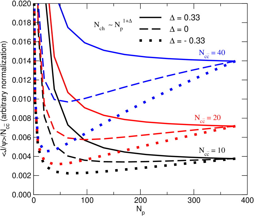
Figure 1: Centrality dependence of binary-scaled $J/\psi$ formation via statistical hadronization.

These features are shown in Fig. 1 for a range of $\Delta$ and $N_{c\bar{c}}(0)$. Aside from the curves for $\Delta={1\over 3}$ which are constant for large $N_{part}$, all of the minimum points are at relatively low values of $N_{part}$, in the region where the statistical hadronization cannot be applied.

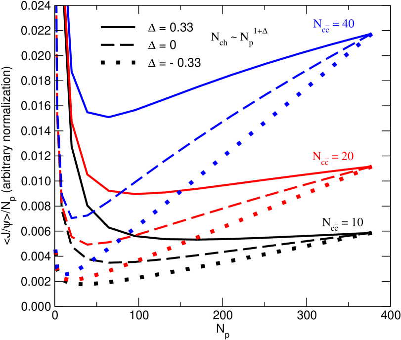
Figure 2: Centrality dependence of participant-scaled $J/\psi$ formation via statistical hadronization.

Figure 2 shows the corresponding behavior for the ratio ${N_{J/\psi}\over N_{part}}$, which can be obtained by making the substitution $\Delta\rightarrow\Delta-{1\over 3}$. The same general behavior is seen, but the sharpness of the approach to the minimum value is enhanced, especially for the largest values of $N_{c\bar{c}}(0)$. The real test of the predicted centrality behavior requires data on both the magnitude of the initial charm production and the centrality dependence of $N_{ch}$.

3 Kinetic formation

The kinetic modelkinetic describes a scenario in which the mobility of initially-produced charm quarks in a space-time region of color deconfinement allow formation of quarkonium via “off-diagonal” combinations of quark and antiquark. The motivation for such a scenario in the case of $J/\psi$ formation has received support from recent lattice calculations of spectral functions. These indicate that $J/\psi$ will exist in an environment at temperatures well above the deconfinement transition lattice1 ; lattice2 . The dominant formation process in this scenario involves the capture of a quark and antiquark in a relative color octet state into the color singlet $J/\psi$ with the emission of a color octet gluon. This reaction is just the inverse of the primary $J/\psi$ dissociation process via collisions with deconfined gluons kharzeevsatz . One can then follow the time evolution of charm quark and charmonium numbers in a region of color deconfinement according to a Boltzmann equation in which the formation and dissociation reactions compete.

$$\frac{dN_{J/\psi}}{d\tau}=\lambda_{\mathrm{F}}N_{c}\,N_{\bar{c}}[V(\tau)]^{-1}-\lambda_{\mathrm{D}}N_{J/\psi}\,\rho_{g}\,,$$ (10)

with $\rho_{g}$ the number density of gluons. The reactivity $\lambda$ is the reaction rate $\langle\sigma v_{\mathrm{rel}}\rangle$ averaged over the momentum distribution of the initial participants, i.e. $c$ and $\bar{c}$ for $\lambda_{F}$ and $J/\psi$ and $g$ for $\lambda_{D}$. The gluon density is determined by the equilibrium value in the QGP at each temperature, and the volume must be modeled according to the expansion and cooling profiles of the interaction region.

This equation has an analytic solution in the case where the total number of formed $J/\psi$ is much smaller than the initial number of $N_{c\bar{c}}$.

$$N_{J/\psi}(\tau_{f})=\epsilon(\tau_{f})[N_{J/\psi}(\tau_{0})+N_{c\bar{c}}^{2}\int_{\tau_{0}}^{\tau_{f}}{\lambda_{\mathrm{F}}\,[V(\tau)\,\epsilon(\tau)]^{-1}\,d\tau}],$$ (11)

where $\tau_{f}$ and $\tau_{0}$ are the final and initial times. The function $\epsilon(\tau_{f})=e^{-\int_{\tau_{0}}^{\tau_{f}}{\lambda_{\mathrm{D}}\,\rho_{g}\,d\tau}}$ would be the suppression factor in this scenario if the formation mechanism were neglected.

One can readily see that $N_{J/\psi}$ obeys the general properties present in Eq. 3. However, the factor equivalent to system volume V (in the statistical hadronization model) is time dependent and modified by a combination of factors involving the interaction rates. Thus the centrality behavior will depend on additional parameters. The initial calculations thewsbielefeld used the ratio of nucleon participants to participant density to define a transverse area which defines the boundary of the region of color deconfinement. This is supplemented by longitudinal expansion starting at an initial time $\tau_{0}$ = 0.5 fm (Transverse expansion was initially neglected, but has been included in subsequent calculations thewssqm2003 .) The expansion was taken to be isentropic, which determines the time evolution behavior of the temperature. The initial value $T_{0}$ is taken as a parameter, and the final $T_{f}$ is fixed at the hadronization point. The reactivities $\lambda_{F}$ and $\lambda_{D}$ require specification of cross sections. For $\sigma_{D}$ we use the “OPE-inspired” model of gluon dissociation of deeply-bound heavy quarkonium peskin kharzeevsatz , which is related via detailed balance to the corresponding $\sigma_{F}$. These cross sections are shown in Fig. 3. One sees that they are peaked at low energy, and that $\sigma_{F}>\sigma_{D}$ due to the large binding energy.

Fig. 4 shows the generic behavior of the $J/\psi$ population resulting from a numerical solution of Equation 10. One can see that the final population is in fact determined by the time integral of the difference between formation and dissociation rates, shown as dashed lines. The magnitudes are determined by the parameter $T_{0}$, which controls the magnitude and time dependence of the gluon density, and also the total lifetime. It is important to note that for parameter values in a range consistent with expectations, the expansion rate of the color deconfinement volume and the decrease of gluon density with time prevent the system from reaching an equilibrium population within this lifetime.

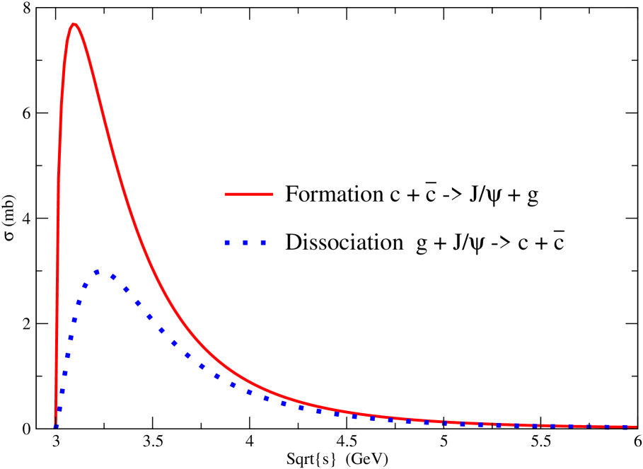
Figure 3: Energy dependence of the OPE-inspired formation and dissociation cross sections for $J/\psi$.

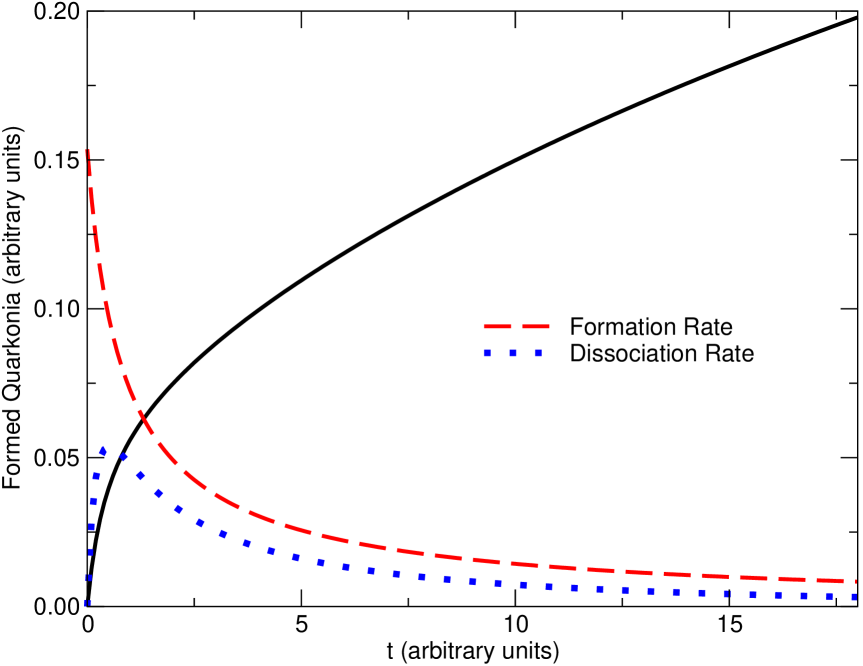
Figure 4: Time development of $J/\psi$ with formation and dissociation rates.

Fig. 5 shows the PHENIX data for $J/\psi$ production in Au-Au collisions at 200 Gev phenixjpsi . The most central bin yield only allowed an upperlimit (hatched horizontal lines), while two less central bins yielded absolute values plus additional one-sigma upper limits both from statistical and systematic uncertainties. The lines shown are calculations in the kinetic model with a range of principal parameters, including $N_{c\bar{c}}$ (b=0), $T_{0}$, transverse expansion velocity (vtr), and in one case an initial population fraction (x) of $J/\psi$. The range of these parameters was chosen to exhibit what constraints are placed by this initial data. All of the calculations used the same charm-quark distribution, which was taken from a LO pQCD calculation mangano . One sees that there is a substantial range of parameters allowed by this data, but that the increase in statistics anticipated in run 3 will allow a much more stringent limit for the acceptable (if any) region of parameter space in the kinetic model.

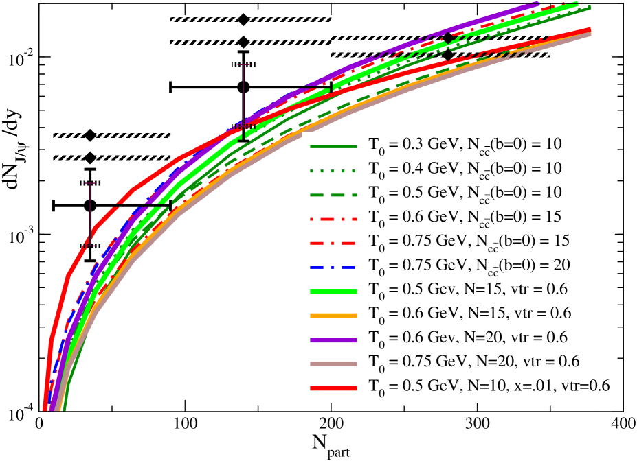
Figure 5: $J/\psi$ formation magnitudes and centrality dependence for 200 GeV Au-Au at RHIC.

The kinetic model also makes predictions for the momentum space distribution of formed $J/\psi$. For this purpose we require the differential cross sections related to the $\sigma_{F,D}$. These are obtained via an adaptation of the corresponding expressions for photodissociation of atomic bound states. One can then express the time-integrated formation rate in terms of a sum over all $c\bar{c}$ pairs, each weighted by differential formation probabilities.

$${{dN_{J/\psi}}\over d^{3}P_{J/\psi}}=\int{{dt}\over{V(t)}}\sum_{i=1}^{N_{c}}\sum_{j=1}^{N_{\bar{c}}}{\it{v}_{rel}}{{d\sigma}\over d^{3}P_{J/\psi}}(P_{c}+P_{\bar{c}}\rightarrow P_{J/\psi}+X)$$ (12)

Note that the formation magnitude exhibits the explicit quadratic dependence on total charm, normalized by a prefactor which is proportional to the inverse of the system volume.

We first look at the rapidity spectra of $c\bar{c}$ pairs, shown in Fig. 6, and compare with the measured $J/\psi$ distribution in pp interactions phenixpp . Normalized spectra are used throughout, so that the results are independent of the prefactors. One sees that the data are consistent with the distribution of unbiased diagonal pairs only, which is what one would expect for pp interactions. The distribution of all pairs (also unbiased) is somewhat narrower than the data. Also shown are all pairs for which each is biased by the total formation probability appropriate for the given pair energy. It is very close to the next curve, which takes into account formation from all pairs, using exact $J/\psi$ kinematics and the full differential dependence. One sees that both of these curves are substantially narrower than the pp data. Thus the kinetic model predicts that the rapidity distribution of $J/\psi$ formed by off-diagonal pairs (only possible in nucleus-nucleus collisions which lead to color deconfinement) will be substantially narrower than $J/\psi$ produced in pp interactions at the same energy.

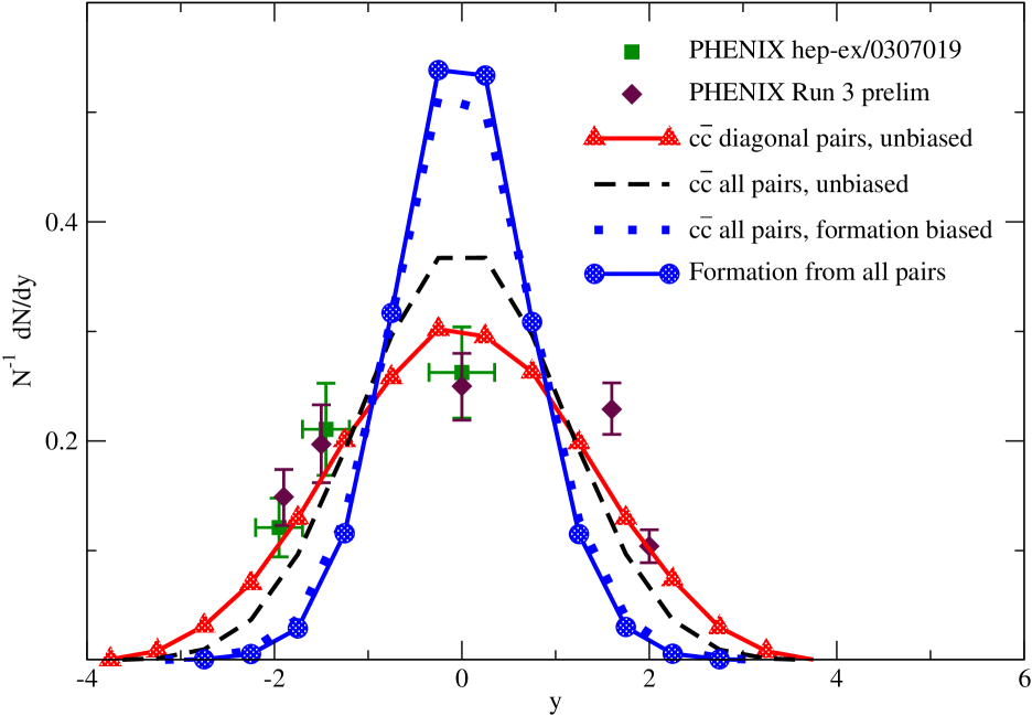
Figure 6: Normalized rapidity spectra of c$\bar{c}$ pairs and $J/\psi$ formation for 200 GeV Au-Au at RHIC.

Fig. 7 shows the transverse momentum spectra of unbiased diagonal $c\bar{c}$ pairs, along with the PHENIX data phenixpp for $J/\psi$ production in pp interactions at 200 GeV. The set of curves result from augmenting the quark initial momenta with a transverse momentum “kick” to simulate confinement and initial state effects. The pp data restricts the magnitude of this kick, parameterized by a Gaussian distribution, to lie within the range $<k_{t}^{2}>_{pp}=0.5\pm 0.1GeV^{2}$. To extend this to formation in Au-Au collisions, we must extract the appropriate $k_{t}$ for initial state effects in the nucleus. We use PHENIX data for $J/\psi$ in d-Au collisions phenixdau , which shows that the $p_{t}$ spectra are broadened relative to that in pp interactions. This results in an estimate for $<k_{t}^{2}>_{Au-Au}=1.3\pm 0.3GeV^{2}$, where the uncertainty is set by the rapidity variation of the $J/\psi$ $p_{t}$ broadening. This range of values was utilized in the formation calculations in Au-Au interactions. The predicted rapidity spectra are found to be essentially independent of the magnitude of the initial charm quark $k_{t}$ kick, so that the narrowest of the curves in Fig. 6 will serve as the kinetic model prediction for $J/\psi$ formed in an Au-Au collision.

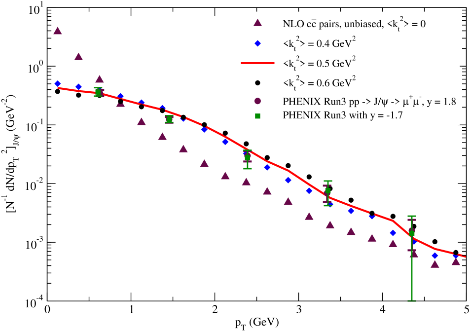
Figure 7: Transverse momentum distribution for diagonal c$\bar{c}$ pairs.

Fig. 8 shows the predicted transverse momentum spectra of $J/\psi$ at RHIC which would result from the formation mechanism, using the entire allowed range of $<k_{t}^{2}>_{Au-Au}$. For comparison we show the distribution of diagonal unbiased $c\bar{c}$ pairs with the central value in the allowed range of initial $<k_{t}^{2}>_{Au-Au}$, which should be relevant if all of the $J/\psi$ were produced directly from the initial $c\bar{c}$ pairs. Of course, both of these distributions would be modified by the competing dissociation process during the expansion phase, but one would anticipate a similar effect on each which would preserve the relative comparison. (A sample suppression factor applied to these curves actually shows very little change in the shape of the normalized spectra.)

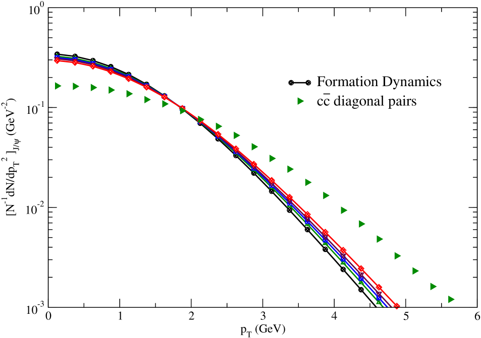
Figure 8: Prediction for $J/\psi$ $p_{t}$ distribution from formation process in Au-Au collisions at RHIC.

4 Summary

One expects on general grounds that heavy quarkonium production in high energy heavy ion collisions must contain a component which is formed either during a period of color deconfinement or at the hadronization point. The magnitude of this formation will increase quadratically with the total amount of charm initially produced via nucleon-nucleon interactions. Both the statistical hadronization model and the kinetic formation model exhibit this property. The absolute magnitude is somewhat model-dependent, and initial RHIC data for $J/\psi$ can be accommodated. The rapidity and transverse momentum spectra may be decisive in determining whether or not this formation makes a significant contribution. The kinetic formation model predicts a narrowing of the $J/\psi$ rapidity distribution (compared with that in pp collisions), and also a narrowing of the transverse momentum distribution (compared with an extrapolation of behavior measured in pp and d-Au collisions). In principle, both of these formation mechanisms can coexist, so that the upcoming Au-Au data may reveal a two-component structure.

- (1) T. Matsui and H. Satz, Phys. Lett. B178 (1986) 416.
- (2) P. Braun-Munzinger and J. Stachel, Nucl. Phys. A690 (2001) 119.
- (3) R. L. Thews, M. Schroedter and J. Rafelski, Phys. Rev. C63 (2001) 054905
- (4) R. Vogt, hep-ph/0412303.
- (5) S. S. Adler et. al. (PHENIX Collaboration), nucl-ex/0409028.
- (6) J. Adams et. al. (STAR Collaboration), nucl-ex/0407006.
- (7) R. L. Thews, Nucl. Phys. A702 (2002) 341.
- (8) A. P. Kostyuk, M. I. Gorenstein, H. Stöcker and W. Greiner, Phys. Rev. C68 (2003) 041902.
- (9) S. S. Adler et. al. (PHENIX Collaboration), Phys. Rev. C69 (2004) 014901.
- (10) A. Andronic, P. Braun-Munzinger, K. Redlich and J. Stachel, Phys. Lett. B571 (2003) 36.
- (11) S. Datta, F. Karsch, P. Petreczky and I. Wetzorke, Phys. Rev. D69 (2004) 094507.
- (12) M. Asakawa and T. Hatsuda, Phys. Rev. Lett. 92 (2004) 012001.
- (13) D. Kharzeev and H. Satz, Phys. Lett. B334 (1994) 155.
- (14) R. L. Thews, J. Phys. G30 (2004) S369.
- (15) M. E. Peskin, Nucl. Phys. B156 (1979) 365; G. Bhanot and M. E. Peskin, Nucl. Phys. B156 (1979) 391.
- (16) M. L. Mangano and R. L. Thews, in preparation.
- (17) S. S. Adler et. al. (PHENIX Collaboration), Phys. Rev. Lett. 92 (2004) 051802.
- (18) Granier de Cassagnac R 2004 (for the PHENIX Collaboration) Preprint nucl-ex/0403030.