Testing saturation with diffractive jet production in deep inelastic scattering

Abstract

We analyse the dissociation of a photon in diffractive deep inelastic scattering in the kinematic regime where the diffractive mass is much bigger than the photon virtuality. We consider the dominant $q\bar{q}g$ component keeping track of the transverse momentum of the gluon which can be measured as a final-state jet. We show that the diffractive gluon-jet production cross-section is strongly sensitive to unitarity constraints. In particular, in a model with parton saturation, this cross-section is sensitive to the scale at which unitarity effects become important, the saturation scale. We argue that the measurement of diffractive jets at HERA in the limit of high diffractive mass can provide useful information on the saturation regime of QCD.

I Introduction

The understanding of diffractive interactions in electron-proton deep inelastic scattering (DIS) has been a great theoretical challenge since diffractive events were observed at HERA h1zeusdata . There exist many attempts to describe the diffractive part of the deep inelastic cross-section within perturbative QCD (for an excellent review, see Ref. heb ). One of the most successful approaches is based on the dipole picture of DIS dipole ; mueller which expresses the scattering of the photon of virtuality $Q^{2}$ through its fluctuation into a color singlet $q\bar{q}$ pair (dipole) of a transverse size $r\!\sim\!1/Q$. That naturally incorporates the description of both inclusive and diffractive events into a common theoretical framework nikzak ; biapesroy , as the same dipole scattering amplitudes enter in the formulation of the inclusive and diffractive cross-sections.

The dipole approach revealed that the total diffractive cross-section is much more sensitive to large-size dipoles than the inclusive one golec . More precisely, it showed that unitarity, and the way it is realized, should be important ingredients of the description of diffractive cross-sections, making those ideal places to look for saturation effects at small-$x$. The saturation parametrization of the dipole scattering amplitude golec was quite successful in describing both the inclusive and diffractive structure functions. In other studies of saturation effects in diffractive DIS, nonlinear evolution equations for the structure function have been derived kovlev ; kovwie , new measurements proposed match , and fits of differents sets of data performed munsho ; forsh .

In this paper, we analyse hard diffraction when the proton stays intact after the collision and the mass $M_{X}$ of the diffractive final state is much bigger than $Q^{2}$. This process is called diffractive photon dissociation. We extend the study of munsho by keeping track of the transverse momentum of the final state partons. We propose the measurement of the final state configuration ${\rm X+jet+gap+p}$ in virtual photon-proton collisions. In order to connect the measured jet with the final-state gluon in our calculations, the jet should form the edge of the rapidity gap. The transverse momentum of the jet provides a hard scale necessary for the use of perturbative QCD, making our calculations valid even at very low values of $Q^{2}$.

We express the diffractive cross-section in terms of dipole scattering amplitudes, using the results derived in cyrille in the eikonal approximation, valid at very high $\gamma^{*}p$ center-of-mass energy. We show that in the context of saturation theory, the transverse momentum distribution of the measured jet is resonant with the scale at which the contributions of large-size dipoles start to be suppressed, called the saturation scale. Using the parametrization golec of saturation effects, we make predictions for the kinematic domain of HERA and exhibit the potential of the diffractive jet production measurement for extracting the saturation scale.

The plan of the paper is as follows. In Section II we recall the derivation of cyrille for the diffractive production of a gluon off a $q\bar{q}$ dipole. In Section III, we derive the cross-section for the diffractive photon dissociation with production of a gluon jet and study its model-independent properties. In section IV, we present the saturation model that we use for the calculation of the jet production cross-section. Section V displays our predictions for the HERA energy range, and Section VI contains conclusions.

II Diffractive gluon production off a $Q\bar{Q}$ dipole

Figure 1: Diffractive gluon production off a $q\bar{q}$ dipole. $x_{0}$ and $x_{1}$ are the transverse coordinates of the quark and antiquark while $k$ and $y$ are the transverse momentum and rapidity of the measured gluon. Black points represent emission of a gluon from the dipole and the vertical wavy lines correspond to a color singlet interaction with a target. The amplitude for the gluon emission after the interaction comes with a minus sign.

In this section we recall the derivation of cyrille of the cross section for the diffractive production of a gluon in the high-energy scattering of a $q\bar{q}$ dipole off an arbitrary target. We shall use the light-cone coordinates with the incoming dipole being a right mover and work in the light-cone gauge $A_{+}=0.$ In such a case, when the dipole passes through the target and interacts with its gauge fields, the dominant couplings are eikonal. The partonic components of the dipole have frozen transverse coordinates, and the gluon fields of the target do not vary during the interaction. This is justified since the incident dipole propagates at nearly the speed of light and its time of propagation through the target is shorter than the natural time scale on which the target fields vary. The effect of the interaction with the target is that the components of the dipole wavefunction pick up eikonal phases.

In Fig. 1 we present the production of a gluon of transverse momentum $k$ and rapidity $y$ off a quark-antiquark dipole with transverse coordinates $x_{0}$ and $x_{1}$. The transverse size of the dipole $|x_{0}\!-\!x_{1}|$ is supposed to be small in order to justify the use of perturbative QCD ($|x_{0}\!-\!x_{1}|\!\ll\!1/\Lambda_{QCD}$). We work in a frame in which the dipole rapidity is not too large so that the radiation of extra softer gluons is described by quantum evolution of the target.

The incident hadronic state is a colorless $q{\bar{q}}$ dipole state which has the following decomposition on the Fock states:

$$|d\,\rangle\,=\,|d\,\rangle_{0}\,+\,|dg\rangle_{0}$$ (1)

where the bare dipole $|d\rangle_{0}$ is characterised by the wavefunction

$$|d\,\rangle_{0}\,=\,\sum_{\alpha\bar{\alpha}}\frac{\delta_{\alpha,\bar{\alpha}}}{\sqrt{N_{c}}}\,|\,(\alpha,x_{0}),(\bar{\alpha},x_{1})\,\rangle$$ (2)

with $\alpha$ and $\bar{\alpha}$ denoting colors of the quark and antiquark, and $x_{0}$ and $x_{1}$ being their transverse positions. The $q\bar{q}g$ part of the dressed dipole $|dg\rangle_{0}$ is characterised by the wavefunction

$$|dg\rangle_{0}\,=\,\frac{1}{\sqrt{N_{c}}}\sum_{\alpha\bar{\alpha}\lambda a}\int d^{2}z\,dy\,\frac{ig_{s}}{\pi}\left[\frac{\epsilon_{\lambda}.(x_{0}\!-\!z)}{|x_{0}\!-\!z|^{2}}-\frac{\epsilon_{\lambda}.(x_{1}\!-\!z)}{|x_{1}\!-\!z|^{2}}\right]T_{\bar{\alpha}\alpha}^{a}\,|\,(\alpha,x_{0}),(\bar{\alpha},x_{1}),(a,\lambda,z,y)\,\rangle\ ,$$ (3)

where $(a,\lambda,z,y)$ characterize gluon color, polarization, transverse coordinate and rapidity, respectively. In addition, $\epsilon_{\lambda}$ is the transverse component of the gluon polarization vector, and $T^{a}$ is a generator of $SU(N_{c})$ in the fundamental representation. The term in brackets in (3) is the well-known wavefunction for the emission of a gluon off a $q\bar{q}$ dipole mueller . The two contributions correspond to emission from the quark and antiquark. The only assumption made to write down (3) is that the gluon is soft, that is its longitudinal momentum fraction with respect to the incident dipole is small. As already mentioned, we work in the frame in which only bare or one-gluon components need to be considered in the wavefunction $|d\,\rangle$. Softer gluons will be included through quantum evolution of the target.

Let us denote by $|t\,\rangle$ the initial state of the target. The outgoing state is obtained from the incoming state $|d\,\rangle\otimes|t\,\rangle$ by the action of the ${\cal S}-$matrix. In the eikonal approximation, ${\cal S}$ acts on quarks and gluons as (see for example coursmuel ; kovwie ; heb ):

$${\cal S}\,(|(\alpha,x)\rangle\!\otimes\!|t\rangle)\,=\,\sum_{\alpha^{\prime}}\left[W_{F}(x)\right]_{\alpha\alpha^{\prime}}|(\alpha^{\prime},x)\rangle\!\otimes\!|t\rangle\ ,\hskip 28.45274pt{\cal S}\,(|(a,\lambda,z,y)\rangle\!\otimes\!|t\rangle)\,=\,\sum_{b}\left[W_{A}(z)\right]^{ab}|(b,\lambda,z,y)\rangle\!\otimes\!|t\rangle\$$ (4)

where phase shifts due to the interaction are described by the eikonal Wilson lines $W_{F}$ and $W_{A}$ in the fundamental and adjoint representations, respectively, corresponding to the propagating quarks and gluons. They are given by the following path ordered exponential

$$W_{F,A}(x)\,=\,{\cal P}\exp\left\{ig_{s}\!\int dz_{+}\,{\cal A}_{-}^{a}(x,z_{+})\,T_{F,A}^{a}\right\}$$ (5)

with ${\cal A}_{-}^{a}$ being the target gauge field, and $T_{F,A}$ are generators of the color group in the fundamental and adjoint representation. Thus, the state $|\Psi_{out}\rangle={\cal S}\,|d\rangle\!\otimes\!|t\rangle$, emerging from the eikonal interaction, is given by

$$|\Psi_{out}\rangle=|\Psi_{1}\rangle+|\Psi_{2}\rangle$$ (6)

with

$$|\Psi_{1}\rangle\!\! = \!\!\frac{1}{\sqrt{N_{c}}}\sum_{\alpha\bar{\alpha}}\left[W_{F}^{\dagger}(x_{1})\,W_{F}(x_{0})\right]_{\bar{\alpha}\alpha}|(\alpha,x_{0}),(\bar{\alpha},x_{1})\rangle\otimes|t\rangle\ ,$$ (7)

$$|\Psi_{2}\rangle\!\! = \!\!\frac{1}{\sqrt{N_{c}}}\sum_{\alpha\bar{\alpha}\lambda b}\int d^{2}z\,dy\ \frac{ig_{s}}{\pi}\left[\frac{\epsilon_{\lambda}\cdot(x_{0}\!-\!z)}{|x_{0}\!-\!z|^{2}}-\frac{\epsilon_{\lambda}\cdot(x_{1}\!-\!z)}{|x_{1}\!-\!z|^{2}}\right]$$ (8)

$$\times\left[W_{F}^{\dagger}(x_{1})\,T^{a}\,W_{F}(x_{0})\right]_{\bar{\alpha}\alpha}\left[W_{A}(z)\right]^{ab}\,|(\alpha,x_{0}),(\bar{\alpha},x_{1}),(b,\lambda,z,y)\rangle\otimes|t\rangle\ .$$

This outgoing state would be the one to consider to compute inclusive cross-sections, as no restrictions on the final state have been imposed. To compute diffractive cross-sections, one has to project the outgoing state $|\Psi_{out}\rangle$ on the subspace of color-singlet states. We have defined diffractive processes as ones in which the target does not break up, therefore one also has to project the outgoing state on the subspace spanned by the target state $|t\rangle$. Those projections are described in detail in cyrille . They create the rapidity gap, preventing the emissions of gluons softer than the one described by (8). Let us denote the resulting state $|\Psi_{diff}\rangle,$ it is given by:

$$|\Psi_{diff}\rangle=|\Psi_{1}^{d}\rangle+|\Psi_{2}^{d}\rangle$$ (9)

with

$$|\Psi_{1}^{d}\rangle\!\! = \!\!\frac{1}{N_{c}}\langle t|\mbox{Tr}{\left({W_{F}^{\dagger}(x_{1})W_{F}(x_{0})}\right)}|t\rangle\,|d\rangle_{0}\otimes|t\rangle\ ,$$ (10)

$$|\Psi_{2}^{d}\rangle\!\! = \!\!\frac{1}{C_{F}N_{c}}\frac{1}{\sqrt{N_{c}}}\sum_{\alpha\bar{\alpha}\lambda a}\int d^{2}zdy\ \frac{ig_{s}}{\pi}\left[\frac{\epsilon_{\lambda}\cdot(x_{0}\!-\!z)}{|x_{0}\!-\!z|^{2}}-\frac{\epsilon_{\lambda}\cdot(x_{1}\!-\!z)}{|x_{1}\!-\!z|^{2}}\right]$$ (11)

$$\times\,\langle t|\mbox{Tr}{\left({W_{F}^{\dagger}(x_{1})\,T^{b}\,W_{F}(x_{0})\,T^{c}}\right)}\left[W_{A}(z)\right]^{bc}|t\rangle\,T^{a}_{\bar{\alpha}\alpha}\,|(\alpha,x_{0}),(\bar{\alpha},x_{1}),(a,\lambda,z,y)\rangle\otimes|t\rangle\ .$$

The state $|\Psi_{2}^{d}\rangle$ represents the first contribution pictured in Fig.1 when the interaction happens after the emission of the gluon. The second contribution when the interaction happens before the gluon emission is part of $|\Psi_{1}^{d}\rangle$. In order to see that, one has to substitute $|d\rangle_{0}\!=\!|d\rangle\!-\!|dg\rangle_{0}$ in $|\Psi_{1}^{d}\rangle:$ the term that comes with $|d\rangle$ is the contribution of elastic scattering while the term that comes with $|dg\rangle_{0}$ and a minus sign represents the second contribution of Fig.1. One can drop the elastic part since it does not contribute to gluon production and write:

$$|\Psi_{diff}\rangle\!\! = \!\!\frac{1}{C_{F}N_{c}\sqrt{N_{c}}}\sum_{\alpha\bar{\alpha}\lambda a}\int d^{2}z\,dy\ \frac{ig_{s}}{\pi}\left[\frac{\epsilon_{\lambda}\cdot(x_{0}\!-\!z)}{|x_{0}\!-\!z|^{2}}-\frac{\epsilon_{\lambda}\cdot(x_{1}\!-\!z)}{|x_{1}\!-\!z|^{2}}\right]\Phi(z)\,T^{a}_{\bar{\alpha}\alpha}\,|(\alpha,x_{0}),(\bar{\alpha},x_{1}),(a,\lambda,z,y)\rangle\otimes|t\rangle$$ (12)

with

$$\Phi(z)=\langle t|\mbox{Tr}{\left({W_{F}^{\dagger}(x_{1})T^{a}W_{F}(x_{0})T^{b}}\right)}W_{A}^{ab}(z)|t\rangle-C_{F}\langle t|\mbox{Tr}{\left({W_{F}^{\dagger}(x_{1})W_{F}(x_{0})}\right)}|t\rangle\ .$$ (13)

From this final state, one calculates the diffractive cross-section for the production of a gluon of transverse momentum $k$ and rapidity $y$ using the following formula:

$$\frac{d\sigma_{diff}}{d^{2}kdy}(x_{01})=\frac{1}{2(2\pi)^{3}}\int d^{2}b\sum_{\lambda=\pm}\sum_{c=1}^{N_{c}^{2}-1}\,\langle\Psi_{diff}|a_{c,\lambda}^{\dagger}(k,y)\,a_{c,\lambda}(k,y)|\Psi_{diff}\rangle$$ (14)

where $a_{c,\lambda}^{\dagger}(k,y)$ and $a_{c,\lambda}(k,y)$ are respectively the creation and annihilation operators of a gluon with color $c$, polarization $\lambda$, rapidity $y$ and transverse momentum $k$. The quantity $x_{01}\!=\!x_{0}\!-\!x_{1}$ is the transverse size of the incoming dipole, and $b\!=\!(x_{0}\!+\!x_{1})/2$ is the impact parameter. The cross-section is computed in details in cyrille , the final result is:

$$\frac{d\sigma^{diff}}{d^{2}kdy}(x_{01})=\frac{\alpha_{s}}{\pi^{2}C_{F}N_{c}^{2}}\int d^{2}b\int\frac{d^{2}z_{1}}{2\pi}\frac{d^{2}z_{2}}{2\pi}\ e^{ik\cdot(z_{2}\!-\!z_{1})}\left[\frac{x_{0}\!-\!z_{1}}{|x_{0}\!-\!z_{1}|^{2}}-\frac{x_{1}\!-\!z_{1}}{|x_{1}\!-\!z_{1}|^{2}}\right].\left[\frac{x_{0}\!-\!z_{2}}{|x_{0}\!-\!z_{2}|^{2}}-\frac{x_{1}\!-\!z_{2}}{|x_{1}\!-\!z_{2}|^{2}}\right]\Phi(z_{1})\Phi^{*}(z_{2})$$ (15)

with $\Phi$ given by formula (13). Making use of the following identity

$$2\mbox{Tr}{\left({W_{F}^{\dagger}(x_{1})\,T^{a}\,W_{F}(x_{0})T^{b}}\right)}\left[W_{A}(z)\right]^{ab}=\mbox{Tr}{\left({W_{F}^{\dagger}(x_{1})W_{F}(z)}\right)}\mbox{Tr}{\left({W_{F}^{\dagger}(z)W_{F}(x_{0})}\right)}-\frac{1}{N_{c}}\mbox{Tr}{\left({W_{F}^{\dagger}(x_{1})W_{F}(x_{0})}\right)}\ ,$$ (16)

one is able to rewrite eq. (13) in terms of the following $\cal{S}-$matrices:

$$S(x_{0},x_{1})=\frac{1}{N_{c}}\langle t|\mbox{Tr}{\left({W_{F}^{\dagger}(x_{1})W_{F}(x_{0})}\right)}|t\rangle$$ (17)

for the scattering of a dipole with the quark and antiquark at transverse coordinates $x_{0}$ and $x_{1}$ respectively, and

$$S^{(2)}(x_{0},z,x_{1})=\frac{1}{N_{c}^{2}}\langle t|\mbox{Tr}{\left({W_{F}^{\dagger}(x_{1})W_{F}(z)}\right)}\mbox{Tr}{\left({W_{F}^{\dagger}(z)W_{F}(x_{0})}\right)}|t\rangle$$ (18)

for the scattering of two dipoles, one with the quark and antiquark at transverse coordinates $x_{0}$ and $z$ and the other with the quark and antiquark at transverse coordinates $z$ and $x_{1}$ . One obtains:

$$\frac{2}{N_{c}^{2}}\Phi(z)=S^{(2)}(x_{0},z,x_{1})-S(x_{0},x_{1})\ .$$ (19)

We have not specified the rapidity dependence of the $\cal{S}-$matrices, it is the rapidity at which the target is evolved. If $Y$ is the total rapidity, then the $\cal{S}-$matrices in $\Phi$ depend on $Y\!-\!y.$

Note that if one considers that the target is a nucleus, and that each scattering on the nucleons happens via a two-gluon exchange, then the target averages in (13) are computable (see e.g. kovwie ) and one recovers the result of kovch . Formulae (15) and (13) are a generalization to any target that includes all numbers of gluon exchanges. Note also that if one writes eq. (19) in terms of $T-$matrices (${\cal{S}}=1-T$), one recovers the two-gluon exchange approximation calculated in bart ; kopdiff by neglecting the term proportional to $T^{2}$. Let us now apply formulae (15) and (13) to diffractive photon dissociation.

III Diffractive photon dissociation

In deep inelastic scattering, a photon of virtuality $Q^{2}$ collides with a proton. In an appropriate frame, called the dipole frame, the virtual photon undergoes the hadronic interaction via a fluctuation into a dipole. The wavefunctions $|\psi^{\gamma}_{T}|^{2}$ and $|\psi^{\gamma}_{L}|^{2}$, describing the splitting of the photon on the dipole, are given by

$$\begin{split}|\psi^{\gamma}_{T}(r,\alpha;Q)|^{2}&=\frac{\alpha_{em}N_{c}}{2\pi^{2}}\sum_{f}e_{f}^{2}\left((\alpha^{2}+(1-\alpha)^{2})\varepsilon_{f}^{2}K_{1}^{2}(\varepsilon_{f}|r|)+m_{f}^{2}K_{0}^{2}(\varepsilon_{f}|r|)\right)\\ |\psi^{\gamma}_{L}(r,\alpha;Q)|^{2}&=\frac{\alpha_{em}N_{c}}{2\pi^{2}}\sum_{f}e_{f}^{2}4Q^{2}\alpha^{2}(1-\alpha)^{2}K_{0}^{2}(\varepsilon_{f}|r|)\end{split}$$ (20)

for a transversely and longitudinally polarized photon, respectively. In the above $\varepsilon_{f}=\sqrt{\alpha(1\!-\!\alpha)Q^{2}\!+\!m_{f}^{2}}$ with $m_{f}$ the mass of the quark $f,$ $r$ is the transverse size of the $q\bar{q}$ pair and $\alpha$ (resp. $1\!-\!\alpha$) is the longitudinal momentum fraction of the antiquark (resp. quark). The dipole then interacts with the target proton and one has the following factorization

$$\sigma^{\gamma^{*}p}=\int d^{2}r\int_{0}^{1}d\alpha\left(|\psi_{T}^{\gamma}(r,\alpha;Q)|^{2}+|\psi_{L}^{\gamma}(r,\alpha;Q)|^{2}\right)\sigma(r,\alpha)$$ (21)

which relates a cross-section for an incident photon $\sigma^{\gamma^{*}p}$ to the corresponding cross-section with an incident dipole $\sigma(r,\alpha).$ In the leading logarithmic approximation we are interested in, the dipole cross-sections do not depend on $\alpha$ and one defines then:

$$\phi(r,Q)\,=\int d\alpha\left(\,|\psi_{T}^{\gamma}(r,\alpha;Q)|^{2}+|\psi_{L}^{\gamma}(r,\alpha;Q)|^{2}\right).$$ (22)

We are going to use the factorization formula (21) to compute the diffractive photon dissociation cross-section.

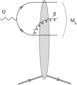
Figure 2: Diffractive photon dissociation in virtual photon-proton collisions. This is the dominant contribution to the diffractive cross-section when the final-state diffractive mass $M_{X}$ is much bigger than the photon virtuality $Q.$

In diffractive deep inelastic scattering, the proton gets out of the collision intact and there is a rapidity gap between that proton and the final state $X,$ see Fig. 2. If the final state diffractive mass $M_{X}$ is much bigger than $Q,$ then the dominant contributions to the final state come from the $q\bar{q}g$ component of the photon wavefunction or from higher Fock states, i.e. from the photon dissociation. By contrast, if $M_{X}\!\ll\!Q,$ the dominant contribution comes from the $q\bar{q}$ component. In this paper we investigate the $q\bar{q}g$ component, in the kinematical region where

$$\beta\equiv\frac{Q^{2}}{Q^{2}+M_{X}^{2}}\ll 1\ .$$ (23)

One can easily express the diffractive mass of the $q\bar{q}g$ final state in terms of the kinematical variables of the partons:

$$M_{X}^{2}=\frac{k^{2}_{q}}{z_{q}}+\frac{k^{2}_{\bar{q}}}{z_{\bar{q}}}+\frac{k_{g}^{2}}{z_{g}}$$ (24)

where $z_{q}$, $z_{\bar{q}},$ and $z_{g}$ are the longitudinal momentum fractions of the quark, antiquark and gluon, respectively, ($z_{q}\!+\!z_{\bar{q}}\!+\!z_{g}\!=\!1$), and $k_{q}$, $k_{\bar{q}},$ and $k_{g}$ are their transverse momenta ($k_{q}\!+\!k_{\bar{q}}\!+\!k_{g}\!=\!0$). Several kinematical configurations can provide $\beta\!\ll\!1,$ however the configuration that gives the dominant contribution to the cross-section is:

$$\frac{k_{g}^{2}}{z_{g}}\gg\frac{k^{2}_{q}}{z_{q}},\ \frac{k^{2}_{\bar{q}}}{z_{\bar{q}}},\ Q^{2}\ .$$ (25)

This is due to the infrared singularity of QCD. Indeed, as we shall see later, this ordering corresponds to the resummation of Feynman diagrams in the leading logarithmic $\log(1/\beta)$ approximation. It also corresponds to a final-state configuration where the gluon jet is the closest to the gap.

In the previous section, we obtained the diffractive cross-section for the production of a gluon with transverse momentum $k$ and rapidity $y$ in the collision of a dipole of tranverse size $x_{01}$ with the target proton in the approximation (25). The result reads

$$\frac{d\sigma^{diff}}{d^{2}kdy}(x_{01})\,=\,\frac{\alpha_{s}N_{c}^{2}}{4\pi^{2}C_{F}}\int d^{2}b\ A(k,x_{0},x_{1};\Delta\eta)\cdot A^{*}(k,x_{0},x_{1};\Delta\eta)$$ (26)

where $x_{0}=b+x_{01}/2$, $x_{1}=b-x_{01}/2$, $Y$ is the total rapidity and $\Delta\eta=Y-y$ is the rapidity gap. The two-dimensional vector $A$ is given by

$$A(k,x_{0},x_{1};\Delta\eta)=\int\frac{d^{2}z}{2\pi}\ e^{-ik\cdot z}\left[\frac{z\!-\!x_{0}}{|z\!-\!x_{0}|^{2}}-\frac{z\!-\!x_{1}}{|z\!-\!x_{1}|^{2}}\right]{\left({S^{(2)}(x_{0},z,x_{1};\Delta\eta)-S(x_{0},x_{1};\Delta\eta)}\right)}$$ (27)

where $S(x_{0},x_{1};\Delta\eta)$ is the elastic ${\cal S}-$matrix for the collision of the dipole $(x_{0},x_{1})$ on the target proton evolved at the rapidity $\Delta\eta$, and $S^{(2)}(x_{0},z,x_{1};\Delta\eta)$ is the elastic ${\cal S}-$matrix for the collision of two dipoles $(x_{0},z)$ and $(z,x_{1})$. These formulae are valid at leading logarithmic accuracy in $y=\log(1/\beta)$ as pointed out before. Indeed, after squaring the term in brackets in (27), one obtains the BFKL kernel. The first (resp. second) term in the brackets corresponds to the emission of the gluon at transverse position $z$ from the quark (resp. antiquark) at transverse position $x_{0}$ (resp. $x_{1}$). The $S^{(2)}$ (resp. $S$) term represents the case where the interaction with the target takes place after (resp. before) the emission of the gluon. We shall refer to it as the real (resp. virtual) term.

Let us introduce the usual kinematics of diffractive DIS: $Y=\log(1/x)$ and $\Delta\eta=\log(1/x_{{\mathbb{P}}})$ with

$$x=\frac{Q^{2}}{Q^{2}+W^{2}}\ ,\hskip 56.9055ptx_{{\mathbb{P}}}=\frac{Q^{2}+M_{X}^{2}}{Q^{2}+W^{2}}\ ,$$ (28)

where $W^{2}$ is the center-of-mass energy of the photon-proton collision. Using the factorization (21), one obtains the $q\bar{q}g$ component of the diffractive cross-section in the virtual photon-proton collision:

$$\frac{d\sigma_{diff}^{\gamma}}{d^{2}k\ dM_{X}}=\frac{2M_{X}}{M_{X}^{2}+Q^{2}}\int d^{2}x_{01}\,\phi(|x_{01}|,Q)\,\frac{d\sigma^{diff}}{d^{2}kdy}(x_{01})\,.$$ (29)

with the photon wavefunction given by formula (22) and the dipole cross-section given by formulae (26) and (27). It is differential with respect to the diffractive mass $M_{X}$ and to the final-state gluon transverse momentum $k,$ which can be identified with the transverse momentum of the jet which is the closest to the rapidity gap. Note that the transverse momentum $k$ provides the hard scale, so that we can apply our formulae to even low values of $Q^{2}.$

Let us make some general comments on the $k-$dependence of the cross-section (29).

• When $k\to 0$.
  The amplitude $A$ given by eq. (27) takes a constant value. The infrared divergences a priori appearing for the virtual term cancel between the $x_{0}$ and $x_{1}$ part and the dominant contribution to $A$ is determined by the large $z$ behavior of $S^{(2)}(x_{0},z,x_{1};\Delta\eta)$. In particular, the value of $z$ at which $S^{(2)}(x_{0},z,x_{1};\Delta\eta)$ starts decreasing to zero plays the role of a natural cutoff and determines the value of $A$. The constant value of the cross-section (29) at $k=0$ is then very sensitive to the way that unitarity sets in.

• When $k\to\infty$.
  The amplitude $A$ decreases as $1/k^{2}$. By changes of variables, one can write

  $$A(k,x_{0},x_{1};\Delta\eta)=\frac{e^{-ik.x_{0}}}{|k|}\int\frac{d^{2}z}{2\pi}\ e^{-ik.z/|k|}\frac{z}{|z|^{2}}{\left({S^{(2)}(x_{0},z/|k|+x_{0},x_{1};\Delta\eta)-S(x_{0},x_{1};\Delta\eta)}\right)}-(x_{0}\leftrightarrow x_{1}).$$ (30)

  Then taking $k\!\rightarrow\!\infty$, and using

  $$S^{(2)}(x_{0},x_{0},x_{1};\Delta\eta)=S^{(2)}(x_{0},x_{1},x_{1};\Delta\eta)=S(x_{0},x_{1};\Delta\eta)\,,$$ (31)

  one sees that the $1/|k|$ term vanishes leaving the dominant contribution behaving as $1\!/\!k^{2}:$

  $$A(k,x_{0},x_{1};\Delta\eta)=\frac{1}{k^{2}}{\left({e^{-ik.x_{0}}\left.\nabla_{z}S^{(2)}\right|_{x_{0}}-e^{-ik\cdot x_{1}}\left.\nabla_{z}S^{(2)}\right|_{x_{1}}}\right)}\ .$$ (32)

  Squaring and integrating the impact parameter one obtains

  $$\frac{d\sigma^{diff}}{d^{2}k\ dy}(x_{01})\,\propto\,\frac{F(|x_{01}|)+G(|x_{01}|)\cos(k\cdot x_{01})}{k^{4}}$$ (33)

  with $F$ and $G$ depending on the precise form of $S^{(2)}.$ When integrating over the angle of $x_{01}$ in (29), the $G$ part becomes suppressed due to the $J_{0}(k|x_{01}|)$ function, and the cross-section then falls as $1/k^{4}$.

These features are general, independent of the form of the ${\cal S}-$matrices. If one looks at the behavior of the observable

$$k^{2}\frac{d\sigma_{diff}^{\gamma}}{d^{2}k\ dM_{X}}$$ (34)

as a function of the gluon transverse momentum $k$, it is going to rise as $k^{2}$ for small values of $k$ and fall as $1/k^{2}$ for large values of $k$. A maximum will occur for a value $k_{0}$ which is related to the inverse of the typical size for which the ${\cal S}-$matrices approach zero; in other words, the maximum $k_{0}$ will reflect the scale at which unitarity sets in. We want to explore this phenomenon in the framework of the theory of parton saturation where unitarity is realized perturbatively.

IV Saturation model for the ${\cal S}-$matrices

The exact form of the ${\cal S}-$matrices is unknown, and we have to consider models in order to produce values of the observable (34) at any value of $k$. For this purpose we consider the following model, inspired by the GBW parameterization golec of parton saturation effects:

$$S(x_{0},x_{1};\Delta\eta)\! = \!\Theta(R_{p}\!-\!|b|)\,\,{\rm e}^{-Q_{s}^{2}(x_{{\mathbb{P}}})x_{01}^{2}/4}\,+\,\Theta(|b|\!-\!R_{p})\ ,$$ (35)

$$S^{(2)}(x_{0},z,x_{1};\Delta\eta)\! = \!\Theta(R_{p}\!-\!|b|)\,\,{\rm e}^{-Q_{s}^{2}(x_{{\mathbb{P}}})(x_{0}\!-\!z)^{2}/4}\,\,{\rm e}^{-Q_{s}^{2}(x_{{\mathbb{P}}})(z\!-\!x_{1})^{2}/4}\,+\,\Theta(|b|\!-\!R_{p})\ ,$$ (36)

where $R_{p}$ is the radius of the proton. $Q_{s}$ is the saturation scale, the basic quantity characterizing saturation effects glr ; glr+ ; mv ; jimwlk . It is a rising function of energy through its $x_{\mathbb{P}}-$dependence. The $b-$dependence of the $S-$ matrices is justified if the dipole sizes $|x_{01}|,$ $|x_{0}\!-\!z|$ and $|z\!-\!x_{1}|$ contribute only when they are much smaller than $R_{p}.$ That is we assume that $x_{{\mathbb{P}}}$ is always such that $Q_{s}(x_{{\mathbb{P}}})\!\gg\!\Lambda_{QCD}$. Note that the model (36) for $S^{(2)}$ neglects correlations between the two dipoles, as it is a product of two $S$’s.

Interestingly enough, since the ${\cal S}-$matrices (35) and (36) are Gaussians, one can analytically compute the amplitude $A$ given by eq. (27). The details of the derivation and the final result (49) are presented in Appendix A. With these results, we obtain for the product $A\cdot A^{*}$:

$$A(k,x_{0},x_{1};\Delta\eta)\cdot A^{*}(k,x_{0},x_{1};\Delta\eta)\,=\,\Theta(|b|\!-\!R_{p})\,\,\frac{x_{01}^{2}}{4k^{2}}\,\,{\rm e}^{-x_{01}^{2}Q_{s}^{2}/2}$$

$$~{}~{}~{}~{}~{}~{}~{}~{}~{}~{}~{}~{}~{}~{}~{}~{}~{}~{}~{}~{}~{}~{}~{}~{}~{}~{}~{}\times\,\frac{\left|2{\left({\cos(k\cdot x_{01}/2)-{\rm e}^{-k^{2}/(2Q_{s}^{2})+\,Q_{s}^{2}x_{01}^{2}/8}}\right)}\ k+\sin(k\cdot x_{01}/2)Q_{s}^{2}\ x_{01}\right|^{2}}{(k^{2}/Q_{s}^{2}-Q_{s}^{2}x_{01}^{2}/4)^{2}+(k\cdot x_{01})^{2}}\,,$$ (37)

where we suppress the dependence of $Q_{s}$ on $x_{{\mathbb{P}}}$ in the notation. Because of the theta function, the $b-$integration in eq. (26) gives a factor $\pi R_{p}^{2}\equiv\sigma_{0}/2$. The result of the integration is then a function of $Q_{s}$ and the two-dimensional vectors $k$ and $x_{01}$. Inserting (LABEL:AA) into (29), one finally writes

$$k^{2}M_{X}\frac{d\sigma_{diff}^{\gamma}}{d^{2}k\ dM_{X}}\! = \!\frac{\alpha_{s}N_{c}^{2}\sigma_{0}}{4\pi^{2}C_{F}}\,\frac{M_{x}^{2}}{M_{x}^{2}+Q^{2}}\int\frac{r\ dr\ d\theta}{(k/(rQ_{s}^{2})-rQ_{s}^{2}/(4k))^{2}+\cos^{2}\theta}\,\,\phi(r,Q)\,\,{\rm e}^{-r^{2}Q_{s}^{2}/2}$$ (38)

$$\times \bigg{[}{\left({\cos{\left({\textstyle{\frac{1}{2}}{kr}\cos\theta}\right)}\,-\,{\rm e}^{-k^{2}/(2Q_{s}^{2})+\,Q_{s}^{2}r^{2}/8}}\right)}^{2}+\frac{Q_{s}^{4}r^{2}}{4k^{2}}\sin^{2}{\left({\textstyle{\frac{1}{2}}{kr}\cos\theta}\right)}$$

$$~{}~{}~{}+\,\frac{rQ_{s}^{2}}{k}\cos\theta\,\sin{\left({\textstyle{\frac{1}{2}}{kr}\cos\theta}\right)}{\left({\cos{\left({\textstyle{\frac{1}{2}}{kr}\cos\theta}\right)}-{\rm e}^{-k^{2}/(2Q_{s}^{2})+Q_{s}^{2}r^{2}/8}}\right)}\bigg{]}$$

where now $k=|k|$, and $\phi(r,Q)$ is given by eq. (22). The $\alpha$-integration to calculate $\phi(r,Q)$ and the integrations over $r$ and $\theta$ can easily be done numerically.

V Numerical analysis and its implications

Let us analyse the $k-$dependence of the diffractive cross-section (38). For this purpose, we define the scaled diffractive cross section

$$\sigma^{scaled}(k,Q^{2},Q_{s})\,=\,\frac{1}{\alpha_{s}\/\sigma_{0}}\,\left(\frac{M_{X}^{2}+Q^{2}}{M_{X}^{2}}\right)M_{X}\,\frac{d\sigma_{diff}^{\gamma}}{d^{2}k\ dM_{X}}\,,$$ (39)

which allows us to leave aside the problem of uncertainties due to $\alpha_{s}$ and $\sigma_{0}.$ The inclusion of $\alpha_{s}$ and $\sigma_{0},$ which have constant values in the kinematical domain we consider here, in the actual observable (34) of course will not change the following discussion. In addition to the gluon transverse momentum $k$, $\sigma^{scaled}$ is a function of two variables: the photon virtuality $Q^{2}$ and the saturation scale $Q_{s}$. We have to keep in mind that the diffractive cross section (38) was derived under the assumption that $M_{X}^{2}\!\gg\!Q^{2}$, thus the factor in the brackets on the r.h.s. of eq. (39) is close to one.

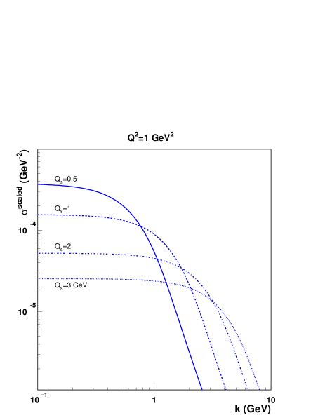
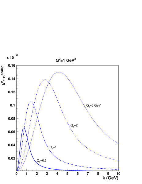
Figure 3: The scaled cross section $\sigma^{scaled}$ and $k^{2}\sigma^{scaled}$ as a function of gluon transverse momentum $k$ for a fixed value of $Q^{2}=1~{}{\rm GeV}^{2}$ and four indicated values of the saturation scale $Q_{s}$.

In Fig.3 we plot $\sigma^{scaled}$ and $k^{2}\sigma^{scaled}$ as a function of $k$, for fixed $Q^{2}\!=\!1~{}{\rm GeV}^{2}$ and four values of the saturation scale, $Q_{s}=0.5,1,2,3~{}{\rm GeV}$. As discussed in section III, independently of the form of the $S-$matrix, $\sigma^{scaled}$ goes to a constant at small momenta while at large momenta $\sigma^{scaled}\sim 1/k^{4}$. We check that this is the case on the first plot. In the model with parton saturation (35) the value of $\sigma^{scaled}$ as $k\!\rightarrow\!0$ is strongly related to the saturation scale $Q_{s}$. This relation is better illustrated on the second plot which represents the dimensionless quantity $k^{2}\sigma^{scaled}$. We see that the transition region between two distinct behaviours at small and large $k^{2}$, which features a marked bump, is linked to the value of $Q_{s}$. It is interesting to explore this observation hoping for the possibility to extract the saturation scale from the measured dependence of the diffractive cross section (34) on the gluon transverse momentum. Of course, in the experimental situation the gluon is seen as a jet. In the kinematic region of high diffractive mass ($\beta\ll 1$) the gluon jet is the closest to the edge of the rapidity gap. The contributions from quark-initiated jets close to the rapidity gap in such a kinematic domain are suppressed by $\log(1/\beta).$

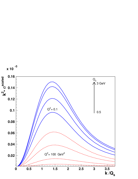
Figure 4: The dimensionless cross section $k^{2}\sigma^{scaled}$ as a function of $k/Q_{s}$ for two extreme values of $Q^{2}$ equal to $0.1$ and $100~{}{\rm GeV}^{2}$. The four curves for each value of $Q^{2}$ correspond to four values of the saturation scale: $Q_{s}=0.5,1,2,3~{}{\rm GeV}$.

In order to quantify the dependence of the position of the maximum of $k^{2}\sigma^{scaled}$ on $Q_{s}$, we plot this cross section as a function of the rescaled transverse momentum $k/Q_{s}$ for the four values of the saturation scale indicated in Fig. 3. In Fig. 4 we show the result of this study for two extreme values of the photon virtuality, $Q^{2}=0.1$ and $100~{}{\rm GeV}^{2}$. As clearly seen, the maximum for each curve is independent of $Q_{s}$ and $Q^{2}$ in a broad range of considered values. From this figure we find that $k_{max}/Q_{s}=1.4\!-\!1.5$, thus within the saturation model, the maximum of $k^{2}\sigma^{scaled}(k)$ is proportional to the saturation scale $Q_{s}$ with a coefficient of proportionality independent of $Q^{2}$. In this way, if the saturation model is accurate, the diffractive gluon production in the domain of large diffractive mass offers a unique opportunity to determine the saturation scale $Q_{s}$ and its dependence on $x_{\mathbb{P}}$.

As already discussed, in the experimental verification of the validity of our description in the $ep$ collisions at HERA, one should consider large-mass diffractive processes ($M_{X}\gg Q$) with a final-state configuration with a jet close to the rapidity gap: ${\rm X+jet+gap+p}$. Then, the diffractive cross section (34) should be determined as a function of the jet tranverse momentum for different values of $x_{\mathbb{P}}$. Positions of the maximum of the measured cross section should be independent of $Q^{2}$, leading to the $x_{\mathbb{P}}-$dependence of the saturation scale. The absolute value of the saturation scale depends of the coefficient of proportionality between $k_{max}$ and $Q_{s}$, which in our model equals $1.4-1.5$. Note that since $k_{max}$ is independent of $Q^{2},$ a wide range of photon virtuality could be used to carry out this measurament, as long as one keeps $\beta\!\ll\!1.$

However, from the experimental point of view there exists an important limitation related to the minimal value of the transverse momentum which could be measured for a jet. In the most pesymistic scenario, considering even rather high values of the saturation scale, $Q_{s}(x_{\mathbb{P}})\sim\!1~{}{\rm GeV}$, it is unlikely that the maximum $k_{max}$ of the cross section (34) can be seen at HERA. Thus, to see the transition between the two different behaviours of the cross section (34) seems like a major experimental challenge.

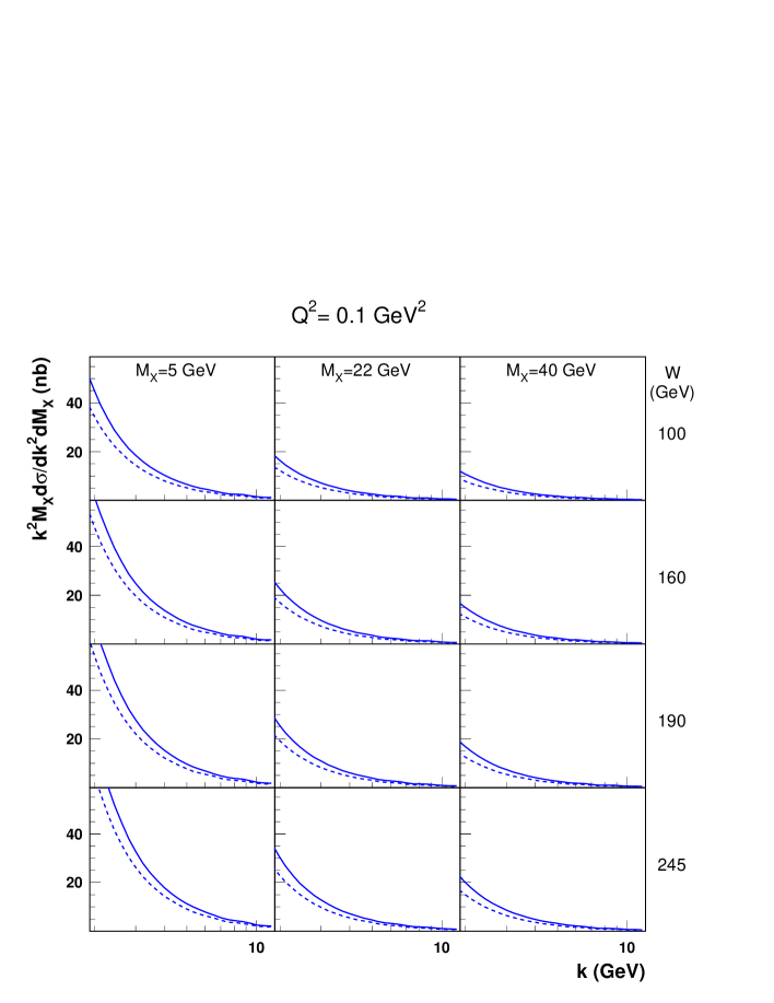
Figure 5: The cross-section $k^{2}M_{X}d\sigma/dk^{2}dM_{X}$ as a function of the jet transverse momentum $k$ for $Q^{2}\!=\!0.1~{}{\rm GeV}$ and different values of diffractive mass $M_{X}$ and energy $W$. Parameters of saturation effects are from golec : solid lines correspond to the case with light quarks only, while the dashed lines are predictions including the charm quark contribution.

In Fig. 5 we illustrated such a situation, when the saturation scale was taken from the model golec in which

$$Q_{s}(x_{\mathbb{P}})=({x_{0}}/{x_{\mathbb{P}}})^{\lambda/2}\ \mbox{GeV}$$ (40)

with the following parameters: $\lambda=0.288~{}(0.277)$ and $x_{0}=3.04\times 10^{-4}~{}(0.4\times 10^{-4})$, where the numbers in parenthesis refer to the case where, in addition to the light quarks, the charm quark is included in (20). The cross-section (38), shown in Fig. 5, is computed for the above saturation scale and the parameters: $\alpha_{s}\!=\!0.15$ and $\sigma_{0}=23.03~{}(29.12)~{}\mbox{mb}$ taken from golec . With these values and the saturation scale (40), the diffractive cross-section (34) integrated over transverse momentum $k$, $d\sigma^{diff}/dM_{X}$, is well described munsho . The values of photon virtuality $Q^{2}$, energy $W$ and diffractive mass $M_{X}$ indicated in Fig. 5 were taken form a recent analysis by the ZEUS Collaboration ZEUSrecent . One sees that, unfortunately, the data should always lie on the perturbative side of the bump. However, it is not necessary to see the whole bump to confirm the influence of the saturation scale on the results. In particular, there is a big difference in the rise towards the bump between the highest $x_{\mathbb{P}}-$bin ($M_{X}\!=\!40~{}{\rm GeV}$ and $W\!=\!100~{}{\rm GeV}$) and the lowest $x_{\mathbb{P}}-$bin ($M_{X}\!=\!5~{}{\rm GeV}$ and $W\!=\!245~{}{\rm GeV}$). A confirmation of such a behaviour would be a sign that the saturation region is indeed close and could lead to the determination of the saturation scale. If however this behaviour is not observed, it could reflect that our saturation model is incomplete, e.g. for example (36) neglects dipole correlations. It could also mean that in this process, unitarity does not come from saturation, but rather from soft physics shaw .

VI Conclusions

Let us summarize the main results of this paper. We analysed the contribution of the $q\bar{q}g$ component of the virtual-photon wavefunction to the diffractive cross sections measured at HERA. In particular, we studied in detail diffractive jet production in the large diffractive mass limit ($\beta\ll 1$) with a jet close to the rapidity gap. In such a case, the jet is initiated by the gluon. We expressed the diffractive photon dissociation cross-section (34) in terms of dipole scattering matrices, formulae (26), (27) and (29). We found that this cross section is strongly sensitive to unitarity constraints. In particular, independently of the form of the scattering matrices, the cross section (34) is a rising (falling) function of the final-state gluon transverse momentum in the limit $k\to 0$ ($k\to\infty$), with the maximum related to the scale at which unitarity effects become important.

In the context of saturation theory in which unitarity is realized perturbatively, the maximum is determined by the saturation scale $Q_{s}$. Using the saturation parametrization (35) and (36) of the scattering matrices, we verify that the relation between the maximum of (34) and the saturation scale is universal, i.e. independent of $Q^{2}$. Therefore, we propose the measurement of the diffractive jet production cross section in $\gamma^{*}p$ collisions at HERA featuring the final-state configuration: ${\rm X+jet+gap+p}$ with a jet close to the rapidity gap. We argue that such a process offers an opportunity to extract the saturation scale from the experiment, provided a low enough jet transverse momentum can be measured.

Appendix A Derivation of the amplitude $A$

In this Appendix, we compute the amplitude (27),

$$A(k,x_{0},x_{1};x_{{\mathbb{P}}})=\int\frac{d^{2}z}{2\pi}\ e^{-ik.z}\left[\frac{z\!-\!x_{0}}{|z\!-\!x_{0}|^{2}}-\frac{z\!-\!x_{1}}{|z\!-\!x_{1}|^{2}}\right]{\left({S^{(2)}(x_{0},z,x_{1};x_{{\mathbb{P}}})-S(x_{0},x_{1};x_{{\mathbb{P}}})}\right)}\ ,$$ (41)

with the ${\cal S}-$matrices given by the saturation model (35). The virtual contribution is proportional to

$$\int\frac{d^{2}z}{2\pi}\ e^{-ik.z}\left[\frac{z\!-\!x_{0}}{|z\!-\!x_{0}|^{2}}-\frac{z\!-\!x_{1}}{|z\!-\!x_{1}|^{2}}\right]=\,{\left({{\rm e}^{-ik\cdot x_{0}}-{\rm e}^{-ik\cdot x_{1}}}\right)}\int\frac{d^{2}z}{2\pi}\ {\rm e}^{-ik\cdot z}\frac{z}{|z|^{2}}\,=-\frac{2k}{|k|^{2}}\,{\rm e}^{-ik\cdot b}\sin\left(\textstyle{\frac{1}{2}}\,k\cdot x_{01}\right)\ .$$ (42)

One can then write

$$A(k,x_{0},x_{1};x_{{\mathbb{P}}})\,=\,\Theta(R_{p}-|b|){\left({{\rm e}^{-ik\cdot x_{0}}\,I(k,x_{01})\,-\,{\rm e}^{-ik\cdot x_{1}}\,I(k,-x_{01})\,+\,\frac{2k}{|k|^{2}}\,{\rm e}^{-ik\cdot b}\,\sin{\left({\textstyle{\frac{1}{2}}\,{k\cdot x_{01}}}\right)}\,{\rm e}^{-Q_{s}^{2}x_{01}^{2}/4}}\right)}$$ (43)

where we have introduced

$$I(k,r)\,=\int\frac{d^{2}z}{2\pi}\ {\rm e}^{-ik\cdot z}\,\frac{z}{|z|^{2}}\,{\rm e}^{-Q_{s}^{2}z^{2}/4}\,{\rm e}^{-Q_{s}^{2}(z+r)^{2}/4}\ .$$ (44)

Introducing $\theta$, the angle between $z$ and $k$, and $\phi$, the angle between $r$ and $k,$ one has:

$$I(k,r)\,=\,{\rm e}^{-Q_{s}^{2}r^{2}/4}\int\frac{d|z|}{|z|}\,{\rm e}^{-Q_{s}^{2}z^{2}/2}\,i\nabla_{k}\int\frac{d\theta}{2\pi}\,{\rm e}^{-i|k||z|\cos\theta-\frac{1}{2}Q_{s}^{2}|z||r|\cos(\theta-\phi)}\ .$$ (45)

The angular integration gives:

$$\int_{0}^{2\pi}\frac{d\theta}{2\pi}\ {\rm e}^{-i|k||z|\cos\theta-\frac{1}{2}Q_{s}^{2}|z||r|\cos(\theta-\phi)}\,=\,\ I_{0}{\left({|z|\sqrt{r^{2}Q_{s}^{4}/4+ik\cdot r\,Q_{s}^{2}\!-\!k^{2}}}\right)}$$ (46)

and differentiating with $i\nabla_{k}$, one obtains

$$I(k,r)=-\frac{ik+r\,Q_{s}^{2}/2}{\sqrt{r^{2}Q_{s}^{4}/4+ik\cdot r\,Q_{s}^{2}\!-\!k^{2}}}\,\,{\rm e}^{-Q_{s}^{2}r^{2}/4}\int_{0}^{\infty}dz\,{\rm e}^{-Q_{s}^{2}z^{2}/2}\,I_{1}{\left({z\sqrt{r^{2}Q_{s}^{4}/4+ik\cdot r\,Q_{s}^{2}\!-\!k^{2}}}\right)}\ .$$ (47)

Then performing the final integration, one gets

$$I(k,r)=\frac{ik+r\,Q_{s}^{2}/2}{k^{2}-r^{2}\,Q_{s}^{4}/4-ik\cdot r\,Q_{s}^{2}}\ e^{-Q_{s}^{2}r^{2}/4}{\left({e^{-\!k^{2}/(2Q_{s}^{2})+r^{2}Q_{s}^{2}/8+ik\cdot r/2}-1}\right)}\ .$$ (48)

Inserting (48) into (43) finally gives:

$$A(k,x_{0},x_{1};x_{{\mathbb{P}}})\! = \!\Theta(R_{p}-|b|)\,{\rm e}^{-ik\cdot b-Q_{s}^{2}x_{01}^{2}/4}\bigg{(}\frac{ik+x_{01}Q_{s}^{2}/2}{k^{2}-x_{01}^{2}Q_{s}^{4}/4-ik\cdot x_{01}\,Q_{s}^{2}}{\left({{\rm e}^{-k^{2}/(2Q_{s}^{2})+x_{01}^{2}Q_{s}^{2}/8}-e^{-ik\cdot x_{01}/2}}\right)}$$ (49)

$$- \frac{ik-x_{01}Q_{s}^{2}/2}{k^{2}-x_{01}^{2}\,Q_{s}^{4}/4+ik\cdot x_{01}Q_{s}^{2}}{\left({{\rm e}^{-k^{2}/(2Q_{s}^{2})+x_{01}^{2}Q_{s}^{2}/8}-{\rm e}^{ik\cdot x_{01}/2}}\right)}+\frac{2k}{|k|^{2}}\sin{\left({\textstyle{\frac{1}{2}}{k\cdot x_{01}}}\right)}\bigg{)}\ .$$

References

• (1) ZEUS Collaboration, M. Derrick et al., Phys. Lett. B315, (1993) 481; H1 Collaboration, T. Ahmed et al., Nucl. Phys. B429, (1994) 477.
• (2) M. Wüsthoff and Alan D. Martin, J. Phys G25 (1999) R309; A. Hebecker, Phys. Rept. 331 (2000) 1.
• (3) N. N. Nikolaev and B. G. Zakharov, Zeit. für. Phys. C49 (1991) 607; Phys. Lett. B332 (1994) 184.
• (4) A. H. Mueller, Nucl. Phys. B415 (1994) 373; A. H. Mueller and B. Patel, Nucl. Phys. B425 (1994) 471; A. H. Mueller, Nucl. Phys. B437 (1995) 107.
• (5) N. N. Nikolaev and B. G. Zakharov, Zeit. für. Phys. C53, (1992) 331.
• (6) A. Bialas, R. Peschanski, Phys. Lett. B378, (1996) 302; Phys. Lett. B387, (1996) 405; A. Bialas, R. Peschanski and C. Royon, Phys. Rev. D57, (1998) 6899.
• (7) K. Golec-Biernat and M. Wüsthoff, Phys. Rev. D59 (1999) 014017; Phys. Rev. D60 (1999) 114023.
• (8) Y. V. Kovchegov and E. Levin, Nucl. Phys. B577 (2000) 221.
• (9) A. Kovner and U. Wiedemann, Phys. Rev. D64, (2001) 114002.
• (10) M. B. Gay Ducati, V. P. Goncalves and M. V. T. Machado, Nucl. Phys. A697 (2002) 767.
• (11) S. Munier and A. Shoshi, Phys. Rev. D69, (2004) 074022.
• (12) J. R. Forshaw, R. Sandapen and G. Shaw, Phys. Lett. B594 (2004) 283.
• (13) C. Marquet, Nucl. Phys. B705 (2005) 319.
• (14) A. H. Mueller, Parton Saturation-an overview, hep-ph/0111244.
• (15) Yu. V. Kovchegov, Phys. Rev. D64, (2001) 114016.
• (16) J. Bartels, H. Jung and M. Wüsthoff, Eur. Phys. J. C11, (1999) 111.
• (17) B. Z. Kopeliovich, A. Schaefer and A. V. Tarasov, Phys. Rev. D62, (2000) 0540022.
• (18) L. V. Gribov, E. M. Levin and M. G. Ryskin, Phys. Rep. 100 (1983) 1.
• (19) A. H. Mueller and J. Qiu, Nucl. Phys. B268 (1986) 427; E. Levin and J. Bartels, Nucl. Phys. B387 (1992) 617.
• (20) L. McLerran and R. Venugopalan, Phys. Rev. D49 (1994) 2233; ibid., (1994) 3352; Phys. Rev. D50 (1994) 2225; A. Kovner, L. McLerran and H. Weigert, Phys. Rev. D52 (1995) 6231; ibid., (1995) 3809; R. Venugopalan, Acta Phys. Polon. B30 (1999) 3731.
• (21) E. Iancu, A. Leonidov and L. McLerran, Nucl. Phys. A692 (2001) 583; Phys. Lett. B510 (2001) 133; E. Iancu and L. McLerran, Phys. Lett. B510 (2001) 145; E. Ferreiro, E. Iancu, A. Leonidov and L. McLerran, Nucl. Phys. A703 (2002) 489; H. Weigert, Nucl. Phys. A703 (2002) 823.
• (22) ZEUS Collaboration; S. Chekanov et al. Study of Deep Inelastic Inclusive and Diffractive Scattering with the ZEUS Forward Plug Calorimeter, DESY-05-011 (January 2005).
• (23) J. R. Forshaw and G. Shaw, JHEP 0412 (2004) 052.