SLAC-PUB-11140

hep-ph/0504210

Limits on Split Supersymmetry from Gluino Cosmology
Asimina Arvanitaki¹, Chad Davis¹, Peter W. Graham¹, Aaron Pierce^2,1, Jay G. Wacker¹

1. Institute for Theoretical Physics

Stanford University

Stanford, CA 94305

2. Theory Group

Stanford Linear Accelerator Center

Menlo Park, CA 94025

An upper limit on the masses of scalar superpartners in split supersymmetry is found by considering cosmological constraints on long-lived gluinos. Over most of parameter space, the most stringent constraint comes from big bang nucleosynthesis. A TeV mass gluino must have a lifetime of less than 100 seconds to avoid altering the abundances of D and ${}^{6}\text{Li}$. This sets an upper limit on the supersymmetry breaking scale $m_{S}$ of $10^{9}$ GeV.

1 Introduction

In split supersymmetry [1, 2] (see also [3]), the superpartner spectrum differs drastically from that of traditional weak scale supersymmetry. The fermionic superpartners are present at the weak scale, while the scalar superpartners have much larger masses, at a scale $m_{S}$. This represents a new scale, which is a priori undetermined. Verification of split supersymmetry will require not only the detection of the new TeV-mass states at colliders, but also the observation of indirect effects of the full supersymmetry present above $m_{S}$.

Most probes of $m_{S}$ are only logarithmically sensitive to this scale [4]. For example, couplings whose values are determined by supersymmetry deviate via renormalization group flow once supersymmetry is broken. The possibility of using such effects to determine $m_{S}$ in split supersymmetry was explored in [1, 5]. There is one observable that has power-law sensitivity to the supersymmetry breaking scale–the gluino lifetime. Thus, measurement of the gluino lifetime would allow a precise determination of $m_{S}$. This motivates us to look at cosmological constraints on the gluino lifetime. For large scalar masses, the gluino can become long-lived. The possibility that the successful predictions of standard big bang cosmology might be altered by a long-lived gluino presents an opportunity to constrain $m_{S}$.

The effects of the late decaying gluinos depend on their annihilation cross section, which determines their relic abundance. The calculation of this cross section is complicated by the strong interactions of the gluino[6, 7]. The relic abundance calculation requires an estimate of non-perturbative annihilation processes after the QCD phase transition. We discuss the computation of the relic abundance of the gluinos in Section 2.

In Section 3, we use the results of this relic abundance calculation to place limits on the gluino lifetime. A particularly strong constraint comes from Big Bang Nucleosynthesis (BBN). We find that for TeV mass gluinos, the lifetime is limited to be less than 100 seconds. Finally, we relate these lifetime bounds to bounds on the scale $m_{S}$.

2 Annihilation of Gluinos

The relic density of gluinos prior to their decay is determined by evolving the Boltzmann equation. This determines the freeze-out temperature where the expansion rate of the universe is balanced against the annihilation rate of the gluinos. There are two regimes of annihilation that we will consider separately. The first era is before the QCD phase transition when there are free gluinos in a QCD plasma. The second era is after the QCD phase transition when the gluinos have become confined in color neutral $R$-hadrons. The annihilation cross section in this second period can, in principle, be much higher than in the first, thus leading to a second period of annihilation.

2.1 Perturbative

The perturbative annihilation of gluinos is well known [6] and at low velocities the cross section is given by

$$\sigma(\tilde{g}\tilde{g}\rightarrow gg)=\frac{27\pi\alpha_{s}^{2}}{64m_{\tilde{g}}^{2}v}+\mathcal{O}(v^{0})\hskip 36.135pt\sigma(\tilde{g}\tilde{g}\rightarrow q\bar{q})=\frac{9N_{f}^{{\text{eff}}}\pi\alpha_{s}^{2}}{64m_{\tilde{g}}^{2}v}+\mathcal{O}(v^{0}),$$ (1)

where $N_{f}^{{\text{eff}}}$ is the effective number of flavors of quarks and includes a phase space suppression for the top quark. We use the full expression for the annihilation cross section [6] in our numerical calculations.

Because the velocities of the gluinos are small at freeze-out, there is a Sommerfeld enhancement due to $t$-channel exchange of multiple gluons [8]. Each loop of gluons gives a $\pi\alpha_{s}/v$ enhancement but can be resummed into an overall enhancement

$$\mathcal{E}_{gg}=\frac{\frac{1}{2}\pi\alpha_{s}/v}{1-\exp(\frac{1}{2}\pi\alpha_{s}/v)}\hskip 36.135pt\mathcal{E}_{q\bar{q}}=\frac{\frac{3}{2}\pi\alpha_{s}/v}{1-\exp(\frac{3}{2}\pi\alpha_{s}/v)}.$$ (2)

Taking the enhancement into account, the cross section becomes

$$\sigma^{\text{tot}}(\tilde{g}\tilde{g}\rightarrow gg)=\frac{27\pi^{2}\alpha_{s}^{3}}{128m_{\tilde{g}}^{2}v^{2}}+\mathcal{O}(v^{-1})\hskip 36.135pt\sigma^{\text{tot}}(\tilde{g}\tilde{g}\rightarrow q\bar{q})=\frac{27N_{f}^{{\text{eff}}}\pi^{2}\alpha_{s}^{3}}{128m_{\tilde{g}}^{2}v^{2}}+\mathcal{O}(v^{-1}).$$ (3)

Because the Sommerfeld enhancement is a long-distance effect, one might worry that this effect is suppressed due to thermal effects from the QCD plasma. However, the effective mass of a gluon in a plasma is $\alpha_{s}T$, while the typical momentum associated with the Sommerfeld enhancement loops is $\alpha_{s}m_{\tilde{g}}v\sim\alpha_{s}\sqrt{m_{\tilde{g}}T}\gg\alpha_{s}T$. Thus, the Sommerfeld enhancement remains effective.

Sommerfeld enhancement can be interpreted as annihilation through off-shell bound states of gluinos. One could also ask whether bound states are formed on-shell. This requires radiating away energy. This will suppress the formation of such states by perturbative powers of $\alpha$. We will revisit bound state formation in a non-perturbative regime in the next section.

2.2 Non-Perturbative

After the QCD phase transition, the gluinos hadronize and form R-hadrons. Very little is certain about the spectroscopy, quantum numbers, or couplings of these strongly interacting particles. In order to have a reliable calculation of the relic density of gluinos, we must nevertheless estimate the annihilation cross section of R-hadrons. Estimates of this cross section have varied widely, due to different assumptions about the relevant hadronic physics. A commonly made assumption is that the annihilation cross section goes as $\pi R^{2}\simeq 1/m_{\pi}^{2}$, where $R$ is the geometric size of the R-hadron. This cross section would be roughly dozens of millibarns, much larger than the perturbative annihilation cross section. In this section we argue that this is not the case. There is a huge separation of scales between the gluino mass and the hadronization scale. This makes it hard to exchange momentum efficiently between the QCD cloud and the gluino core. Thus, we expect the light QCD degrees of freedom to decouple from the annihilation process.

Geometric ($\sigma\sim R^{2}$) cross sections for $R$-hadron scattering are applicable in the case of $q^{2}<\Lambda_{QCD}^{2}$. Such processes do not probe the interior structure of the hadron because they transfer low momentum, and the hadron appears like a solid object. On the other hand, gluino annihilation is a large momentum transfer process and probes the interior structure of the hadron. The partonic picture of the hadron becomes relevant, and we expect the annihilation cross section is set by the size of the parton, $\sigma_{ann}\sim m_{\tilde{g}}^{-2}$.

To explore this further, we can rely on simple quantum mechanical scattering arguments. Despite the strong dynamics, the inelastic $R$-hadron cross section must still satisfy partial wave unitarity [9]

$$\sigma_{j}^{inel}\leq\frac{\pi}{m_{\tilde{g}}^{2}v^{2}}(2j+1).$$ (4)

Notice that the cross section scales as the de Broglie wavelength of the gluino rather than a geometric quantity. However, this does not prove that the annihilation cross section scales as $(m_{\tilde{g}}v)^{-2}$. If many partial wave cross sections contribute, they can add up to a geometric cross section. For example, if all partial waves up to $j_{\text{max}}=m_{\tilde{g}}vR$ contribute, where $R$ is the size of the R-hadron, then Eqn. 4 sums to give a geometric cross section,  $R^{2}$. For this to occur, high angular momentum partial waves must contribute (i.e. $j\simeq 30$ for a TeV scale gluino at temperatures around $\Lambda_{\text{QCD}}$). However, for these high angular momentum modes to lead to annihilation, the gluinos must effectively tunnel through a large barrier. This means that direct annihilation is exponentially suppressed for high $j$. A significant annihilation cross section through larger angular momentum partial waves typically requires either that the object be of uniform density (i.e. like a macroscopic composite system) or that there are high angular momentum bound states that contribute to the cross section.

One potential way to avoid the tunneling suppression at large angular momenta would be via the exchange of a high $j$ QCD resonance. In this case, the resonance itself would carry the angular momentum, and could lead to immediate annihilation. While this might be plausible if the gluinos had a mass in the GeV range, it does not seem plausible for TeV mass gluinos– there are no sharp QCD resonances well above the GeV scale. If such a resonance were to exist, it would be extraordinarily broad, and would therefore not lead to rapid resonant annihilation.

A second way to bleed off angular momentum would be by radiating. For the relevant large angular momentum states, we can use a semi-classical treatment where radiation is caused by accelerating a particle. This acceleration could be caused if a QCD string formed between the two gluinos. In this case, the radiation may be described via the Larmor formula where the power radiated is

$$P\sim a^{2}\sim\frac{1}{(\alpha^{\prime}m_{\tilde{g}})^{2}},$$ (5)

where $\alpha^{\prime}$ is the tension of the exchanged QCD string. The total energy radiated can be estimated by multiplying this power by the crossing time $t_{cross}\sim R/v$, where $v$ represents the relative velocity of the two hadrons. For $T\sim\Lambda_{QCD}$, we find

$$E_{rad}\sim\left(\frac{\Lambda_{QCD}}{m_{\tilde{g}}}\right)^{3/2}\Lambda_{QCD}.$$ (6)

Thus, radiation from the gluinos is small, in fact, much less than the mass gap to the lightest possible state that could be radiated (the pion). This agrees with the intuition that heavy objects do not radiate. We should note that we could have applied a similar Larmor argument prior to the QCD phase transition. In this case, the relevant force is not due to a QCD string, but rather to a QCD Coulomb potential. In this case, the radiation will be further suppressed by perturbative powers of $\alpha_{s}$, again arguing against a large rate for the formation of bound states. Light QCD degrees of freedom do not carry the momentum or angular momentum of the system. Radiation from the cloud therefore is not able to reduce the relative angular momentum of the heavy gluinos, so they remain incapable of direct annihilation.

2.3 Relic Abundance Summary

Figure 1: Gluino abundance per co-moving volume as a function of mass. Three curves are shown. In the first (solid), the annihilation cross section is assumed to be simply given by the perturbative cross section of Eqn. 3. The other curves correspond to a cross section that saturates $s$-wave (dashed) and $s$-wave plus $p$-wave unitarity (dot-dashed).

In summary, we estimate the total annihilation cross section as follows: for $T>\Lambda_{QCD}$, we simply utilize the perturbative cross section for gluinos [6]; for $T<\Lambda_{QCD}$, we allow for the possibility of an increased cross section. However, because we have argued that high angular momentum states do not significantly contribute to the annihilation of gluinos, we do not allow for an arbitrarily large cross section at this stage. We expect that the annihilation is conservatively given by a cross section that saturates s-wave unitarity. We take $\Lambda_{QCD}=200$ MeV as the point where the cross section changes.

This cross section is thermally averaged [10] and used in the numerical integration of the Boltzmann equation. We treat the QCD phase transition as second order although this is not expected to significantly affect the results [11].

For completeness, in Fig. 2, we show the relic abundance for three cases. First, a solid curve that shows the relic abundance, assuming all annihilation is perturbative. Second, a dashed curve that incorporates the turn on of a cross section that saturates $s$-wave unitarity. Finally, a dot-dashed curve that has a cross section that saturates $s$-wave plus $p$-wave unitarity, which we view as an even more conservative assumption.

3 Limits

In this section we discuss the effects of the decays of the relic gluinos. Depending upon the lifetime of the gluino, these decays can disturb the predictions of BBN, distort the Cosmic Microwave Background Radiation (CMBR), or show up in the diffuse gamma ray background. If the gluinos have a lifetime of order the age of the universe, they can potentially be observed in experiments searching for heavy exotic nuclei. We now discuss each of these constraints.

First, we consider the era of BBN. These constraints are a function of the gluino destructive power, $\xi\equiv E_{vis}Y$. Here $E_{vis}$ is the energy of the gluino decay products which are deposited in the thermal bath, and $Y\equiv n/s$ represents the number density of gluinos per co-moving volume. To determine $E_{vis}$, we assume that half of the energy of a decaying gluino goes into the neutralino, while the other half is distributed between hadrons. At the time of the gluino decay, the neutralino mean free path is large, and thus the energy in the neutralino is simply carried away; it is not “visible”. That is to say, we are taking the visible energy $E_{vis}=m_{\tilde{g}}/2$. If the lightest supersymmetric particle has a mass close to that of the gluino, the limits are weakened for a given abundance.

Constraints arising from BBN on the lifetime of a hadronically decaying particle as a function of its destructive power were described in [12]. We take the most conservative D/H and ${}^{4}\text{He}$ limits. We are interested in the limits as a function of the gluino mass, but they only present results for three masses (100 GeV, 1 TeV, and 10 TeV). For a fixed lifetime, the dependence of $\xi$ on $m_{\tilde{g}}$ is roughly power-law, and so we can use these three points to interpolate to different values of the gluino mass. This procedure gives bounds on the gluino lifetime as a function of mass. We then convert lifetime bounds to bounds on the supersymmetry breaking scale [13, 14], augmenting the decay rate by the two-body decay rate when significant. The result is shown in Fig. 2.

We now discuss in more detail the origin of the BBN bounds. Three BBN bounds are particularly restrictive: D/H, ${}^{6}\text{Li/H}$, and ${}^{3}\text{He/D}$. After BBN has finished, the universe is composed primarily of hydrogen and helium, with trace amounts of other elements. A gluino decay releases particles at energies much higher than the typical kinetic energies of nuclei at that time. At times later than about 100 seconds, mesons decay before they scatter, so the most destructive hadronic decay products are baryons. Protons produced by gluino decays scatter off of the background protons and ${}^{4}\text{He}$ nuclei. The elastic scattering increases the energy of background protons, making them more likely to react with other elements. The inelastic $\text{p}+{}^{4}\text{He}\rightarrow{}^{3}\text{He}+\text{D}$ reaction increases D/H. If a D scatters off of a background ${}^{4}\text{He}$ nucleus, ${}^{6}\text{Li}$ can form. The epoch important for D formation is around 100 seconds – this sets the lower edge of the BBN curve in Fig. 2.

A second process important in BBN is photo-dissociation[15]. Photons with energies above 20 MeV can break ${}^{4}\text{He}$ nuclei into ${}^{3}\text{He}$ or Tritium (which later decays weakly to ${}^{3}\text{He}$). This can cause the ${}^{3}\text{He/D}$ ratio to become too large. However, this process does not become important until the temperature drops to $\sim 1$ keV at $\sim 10^{6}$ seconds (see, e.g. [16]). At temperatures before this, the 20 MeV photons lose energy efficiently by scattering off the background photons before they can break apart a nucleus.

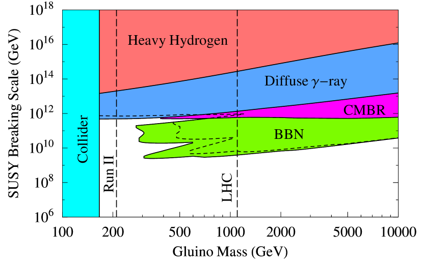
Figure 2: Limits on the supersymmetry breaking scale, $m_{S}$, as a function of the gluino mass, $m_{\tilde{g}}$. The bounds are derived assuming a perturbative cross section in Eqn.  3 for temperatures greater than the QCD phase transition, $T>200$ MeV. For $T<200$ MeV, we assume that the annihilation cross section saturates $s$-wave unitarity. Also shown (dashed) are the limits in the case where the annihilation cross section saturated $s$-wave plus $p$-wave unitarity. The shaded regions are excluded. The lower edge of the BBN curve arises from the requirement that the $D/H$ ratio remained undisturbed, and corresponds to a lifetime of approximately 100 seconds.

Gluinos that decay after recombination can give rise to photons that free-stream to us, and are visible in the diffuse gamma ray background [17]. Photons are produced when gluinos decay to pions which subsequently decay to gamma rays. Observations by EGRET[18] and COMPTEL limit the flux of these gamma rays and thus the relic abundance of gluinos. A 3-body decay including an invisible product, in our case the neutralino, was assumed in [17]. This is also the case at hand. The region excluded is shown in Fig. 2. These observations of the diffuse gamma ray background rule out a gluino with lifetime around the present age of the universe.

The CMBR can be used to put further limits on the relic abundance of gluinos with lifetimes up to $\sim 10^{13}$ s [19, 20]. Gluinos that decay during or after the epoch of thermalization of the CMBR can distort its spectrum and are thus limited by observations from COBE[21]. To derive these limits we make the conservative assumption that roughly $10\%$ of the energy of the gluino gets transmitted to the CMBR when it decays, with the remainder carried off by neutrinos or the lightest supersymmetric particle. The limits derived from these constraints are shown in Fig. 2.

If the gluino lives to the present day we would expect it to bind into nuclei, producing anomalously heavy isotopes. A combination of time of flight, mass spectrometry, and direct density measurements places severe limits on the abundance of terrestrial heavy elements today [22, 23]. This rules out a gluino with lifetime greater than the present age of the universe for the entire gluino mass range considered. These bounds are weakened if it is assumed that the heavy elements sink towards the center of the earth. However, for heavy hydrogen, the equilibrium time constant is $\gtrsim 10^{8}$ years and so if the oceans undergo mixing the heavy hydrogen would be roughly uniformly distributed [22]. The bounds derived from these searches are shown in Fig. 2, labeled “Heavy Hydrogen.”

Gluino properties are already restricted via direct searches at colliders[24, 25]. The weakest limits come in the case where the produced $R$-hadrons are neutral. Then, they escape the detector, carrying away a substantial fraction of the event energy. The gluinos are then observed in mono-jet events, triggered by the presence of an additional radiated jet. Current limits on the gluino from Tevatron Run I are $m_{\tilde{g}}>170~{}\text{GeV}$ [25]. This bound should increase to $210~{}\text{GeV}$ if Run II sees nothing, and to $1100~{}\text{GeV}$ at the Large Hadron Collider (LHC). These bounds are independent of the supersymmetry breaking scale. If charged $R$-hadrons are produced that do not immediately decay, this bound improves. Searching for gluinos through anomalously slow tracks in the tracking chambers of both ATLAS and Tevatron were studied in [26, 27]. These provide search reaches comparable to the monojet signal and will be useful as an additional discovery channel.

Finally there is the possibility of seeing gluinos in cosmic rays and was studied by [28]. If a gluino were seen, then this would set and lower limit on the susy breaking scale. While most of the available lifetime and mass ranges are ruled out by the considerations in this paper, there is a window available at low gluino masses for gluinos to be seen in cosmic rays.

4 Conclusion

In this note we have explored the limits on the split supersymmetry parameter space coming from cosmological constraints on a long lived gluino. If the gluino were to annihilate with a geometric cross section after the QCD phase transition, then it would evade most cosmological constraints. However, we have argued that this is not the case, the cross section is more likely set by the de Broglie wavelength of the gluino. Then, the cross section is likely bounded by saturating s-wave unitarity. Using this cross section, it is possible to extract useful limits from the CMBR, BBN, and the diffuse gamma ray background. For gluinos heavier than 300 GeV the earliest cosmological constraints are from BBN, specifically the D/H ratio. This sets an upper bound to the lifetime of roughly 100 seconds and an upper bound on $m_{S}$ of $10^{9}$ GeV. For gluinos lighter than 300 GeV, the earliest constraints arise from non-observation of diffuse gamma rays and sets an upper limit to the lifetime of $10^{6}$ years and corresponds to $m_{S}<10^{11}$ GeV. If collider searches at the LHC find a gluino heavier than 600 GeV, then the lifetime will be less than 100 seconds. This has implications for experiments that hope to trap the gluino and directly measure its lifetime.

References

- [1] N. Arkani-Hamed and S. Dimopoulos, arXiv:hep-th/0405159.
- [2] G. F. Giudice and A. Romanino, Nucl. Phys. B 699, 65 (2004) [Erratum-ibid. B 706, 65 (2005)] [arXiv:hep-ph/0406088].
- [3] J. D. Wells, arXiv:hep-ph/0306127.
- [4] H. C. Cheng, J. L. Feng and N. Polonsky, Phys. Rev. D 56, 6875 (1997) [arXiv:hep-ph/9706438].
- [5] A. Arvanitaki, C. Davis, P. W. Graham and J. G. Wacker, Phys. Rev. D 70, 117703 (2004) [arXiv:hep-ph/0406034].
- [6] H. Baer, K. m. Cheung and J. F. Gunion, Phys. Rev. D 59, 075002 (1999) [arXiv:hep-ph/9806361].
-
[7]
S. Wolfram,
Phys. Lett. B 82, 65 (1979);
C. B. Dover, T. K. Gaisser and G. Steigman, Phys. Rev. Lett. 42, 1117 (1979);
R. N. Mohapatra and S. Nussinov, Phys. Rev. D 57, 1940 (1998) [arXiv:hep-ph/9708497]. -
[8]
T. Appelquist and H. D. Politzer,
Phys. Rev. Lett. 34, 43 (1975);
S. J. Brodsky, J. F. Gunion and D. E. Soper, Phys. Rev. D 36, 2710 (1987). - [9] K. Griest and M. Kamionkowski, Phys. Rev. Lett. 64, 615 (1990).
- [10] P. Gondolo and G. Gelmini, Nucl. Phys. B 360, 145 (1991).
- [11] M. Srednicki, R. Watkins and K. A. Olive, Nucl. Phys. B 310, 693 (1988).
- [12] M. Kawasaki, K. Kohri and T. Moroi, Phys. Rev. D 71, 083502 (2005) [arXiv:astro-ph/0408426].
- [13] M. Toharia and J. D. Wells, arXiv:hep-ph/0503175.
- [14] P. Gambino, G. F. Giudice and P. Slavich, arXiv:hep-ph/0506214.
- [15] J. R. Ellis, G. B. Gelmini, J. L. Lopez, D. V. Nanopoulos and S. Sarkar, Nucl. Phys. B 373, 399 (1992).
- [16] M. Kawasaki and T. Moroi, Astrophys. J. 452, 506 (1995) [arXiv:astro-ph/9412055].
- [17] G. D. Kribs and I. Z. Rothstein, Phys. Rev. D 55, 4435 (1997) [Erratum-ibid. D 56, 1822 (1997)] [arXiv:hep-ph/9610468].
- [18] P. Sreekumar et al. [EGRET Collaboration], Astrophys. J. 494, 523 (1998) [arXiv:astro-ph/9709257].
- [19] W. Hu and J. Silk, Phys. Rev. Lett. 70, 2661 (1993).
- [20] J. L. Feng, A. Rajaraman and F. Takayama, Phys. Rev. D 68, 063504 (2003) [arXiv:hep-ph/0306024].
- [21] D. J. Fixsen, E. S. Cheng, J. M. Gales, J. C. Mather, R. A. Shafer and E. L. Wright, Data Astrophys. J. 473, 576 (1996) [arXiv:astro-ph/9605054].
- [22] P. F. Smith, J. R. J. Bennett, G. J. Homer, J. D. Lewin, H. E. Walford and W. A. Smith, Nucl. Phys. B 206, 333 (1982).
- [23] T. K. Hemmick et al., Phys. Rev. D 41, 2074 (1990).
- [24] W. Kilian, T. Plehn, P. Richardson and E. Schmidt, Eur. Phys. J. C 39, 229 (2005) [arXiv:hep-ph/0408088].
- [25] J. L. Hewett, B. Lillie, M. Masip and T. G. Rizzo, JHEP 0409, 070 (2004) [arXiv:hep-ph/0408248].
- [26] A. C. Kraan, Eur. Phys. J. C 37, 91 (2004) [arXiv:hep-ex/0404001]. A. C. Kraan, arXiv:hep-ex/0506009.
- [27] R. Culbertson et al. [SUSY Working Group Collaboration], arXiv:hep-ph/0008070.
- [28] L. Anchordoqui, H. Goldberg and C. Nunez, Phys. Rev. D 71, 065014 (2005) [arXiv:hep-ph/0408284].