IFJPAN-V-04-06
CERN-PH-TH/2005-065

Non-Markovian Monte Carlo Algorithm for the Constrained Markovian Evolution in QCD^⋆

S. Jadach and M. Skrzypek

Institute of Nuclear Physics, Polish Academy of Sciences,
ul. Radzikowskiego 152, 31-342 Cracow, Poland
and

CERN Department of Physics, Theory Division
CH-1211 Geneva 23, Switzerland

We revisit the challenging problem of finding an efficient Monte Carlo (MC) algorithm solving the constrained evolution equations for the initial-state QCD radiation. The type of the parton (quark, gluon) and the energy fraction $x$ of the parton exiting emission chain (entering hard process) are predefined, i.e. constrained throughout the evolution. Such a constraint is mandatory for any realistic MC for the initial state QCD parton shower. We add one important condition: the MC algorithm must not require the a priori knowledge of the full numerical exact solutions of the evolution equations, as is the case in the popular “Markovian MC for backward evolution”. Our aim is to find at least one solution of this problem that would function in practice. Finding such a solution seems to be definitely within the reach of the currently available computer CPUs and the sophistication of the modern MC techniques. We describe in this work the first example of an efficient solution of this kind. Its numerical implementation is still restricted to the pure gluon-strahlung. As expected, it is not in the class of the so-called Markovian MCs. For this reason we refer to it as belonging to a class of non-Markovian MCs. We show that numerical results of our new MC algorithm agree very well (to $0.2\%$) with the results of the other MC program of our own (unconstrained Markovian) and another non-MC program QCDnum16. This provides a proof of the existence of the new class of MC techniques, to be exploited in the precision perturbative QCD calculations for the Large Hadron Collider.

To be submitted to Acta Physica Polonica

IFJPAN-V-04-06
CERN-PH-TH/2005-065

^⋆Supported in part by the EU grant MTKD-CT-2004-510126, in partnership with the CERN Physics Department.

1 Introduction

The unprecedented experimental precision of the forthcoming experiments at the Large Hadron Collider (LHC), in terms of apparatus resolution and event statistics, will have to be matched by a far better precision of the theoretical calculations in the strong interaction sector than available at present. The well established theory of strong interactions, Quantum Chromodynamics (QCD), is in principle able to provide very precise predictions for the high energy scale (mass, transverse momentum, momentum transfer) processes. The perturbative predictions of QCD are obtained within one of two very different calculational frameworks: the so-called matrix element (ME) calculations and models of the parton shower (PS) type implemented in the Monte Carlo (MC) event generators. For a more detailed review of these methods, see for example ref. [1]. In the ME calculations the basic ingredients are real- and virtual-emission matrix elements evaluated in the fixed-order perturbative QCD, for the hard process at the high energy scale, embedded in the standard Lorenz-invariant phase space (LIPS). The fixed-order ME is combined with the parton distributions (PDFs) describing lower energy multiple emissions in an inclusive manner (integrated over the transverse momenta). On the other hand, the PS framework offers a fully exclusive picture, down to hadronization energy scale, that is the true MC events with explicit 4-momenta, for all multiple soft and collinear emissions associated with the hard process – the same emissions as are encapsulated in the PDFs of the ME approach. However, the classic PS implements the hard process only at the Born (tree) level.

The above two complementary approaches have their strong and weak points of their own. Without entering into details, we may safely say that it is absolutely mandatory to combine the virtues of the two approaches if one hopes to ever achieve a significant improvement of the precision of the QCD predictions, for a wide class of observables (not only total rates); see conclusions of ref. [1].

There were numerous attempts to combine ME calculations with the parton shower approach beyond the leading order, the most elaborate being the recent one of Frixione and Webber [2]. However, none of them are fully satisfactory and there are more proposals in this direction; see for instance ref. [3]. There seems to be a growing consensus that part of the problem is in the fundamental formulation of the PS models implemented in the PS MC. All these models are of the Markovian type, in which the branching process (the binary decay of the parton) continues until the boundary of the phase space is hit; the number of branchings (emissions) is known at the very end of the branching process. This is in stark contrast to the ME approach, where the number of partons involved is defined at the very beginning, and the integral over standard LIPS is evaluated for a given ME. In this sense, the ME approach is basically non-Markovian – this is one of the (principal) sources of the difficulties in combining the ME and PS approaches.

In this paper we do not offer any “silver bullet” solution of the above problems. However, we provide one possibly useful cornerstone, in constructing yet another class of methods of combining ME and PS methodologies. Our aim is to provide the means of reformulating the PS model and the corresponding MC algorithm in a non-Markovian way. In fact, we restrict ourselves to an even narrower, but well defined subject of solving QCD DGLAP [4] evolution equations using the MC method, which is at the heart of any PS MC modelling. We also show, for the initial-state PS (IS PS), that the non-Markovian solution of the DGLAP evolution equations emerges in a natural way as an alternative solution to yet another long-standing difficulty in the PS MC modelling: the problem of the energy constraint. The energy constraint in the IS PS is the requirement of constraining to a predefined value the energy of the parton entering the hard process. This is so because of a selective nature of the typical hard process ME, typically due to narrow resonances. In the typical Markovian PS MC the energy of a parton entering the hard process results from many branchings and it is impossible to put any constraint on it, in the same way as it is impossible to predefine the number of branchings or the type of the parton (quark or gluon) at the end of the branching process. The well known and widely adopted work-around is the so-called “Markovian MC for the backward evolution” of Sjöstrand [5]. We shall show that there exists yet another class of MC algorithms with the energy constraint, which turns out to be non-Markovian in a natural way.

Summarizing, the motivation of our search for non-Markovian modelling of the QCD evolution equations is that: (a) it is closer to the ME approach, (b) it solves the energy constraint problem in the IS PS in a novel way, with potential advantages of its own, as discussed below.

This paper is one of several related works done in parallel, exploiting various aspects of the Markovian-type and non-Markovian-type MC solutions of the QCD evolution equations. Basic results of the present work were presented in the conference contributions quoted in ref. [7]. The earlier work of ref. [8] presents precision MC evaluations of the LL QCD evolution equations using an unconstrained Markovian MC. Although the Markovian calculations of refs. [8, 9] are not our main aim, they form a very valuable baseline (benchmark) for the constrained non-Markovian calculations, as the ones presented here.

This work presents the first successful MC algorithm in the constrained non-Markovian class, although restricted to the pure gluon-strahlung in the actual numerical implementation. Later on, the authors of this paper have found yet another family of MC algorithms, in the same important class of non-Markovian constrained MCs, which will be described in the forthcoming ref. [10], and are even more efficient and easier to implement. However, at this early stage it makes perfect sense to collect all possible non-Markovian MC algorithms for the QCD evolution equations, simply because it is difficult to foresee which of them will be most adequate in the future attempts at combining PS and ME calculations. In other words, the richer the menu of the different non-Markovian algorithms at our disposal, the better.

The plan of the paper is the following: in the next section we elaborate more on our aims and the general framework of our work. In section 3 we formulate in detail several examples of the constrained evolution MC algorithms, and present numerical tests of the corresponding computer implementations. A short summary concludes the main result. The appendix contains the algebra related to the MC method (multibranching) employed in section 3.

2 MC solutions for QCD evolution equations

As was already said, we are looking for any possibly non-Markovian, MC solution of the QCD evolution equations, with the constraint on the final parton type and its $x$, the energy fraction. Needless to say, for a given $x$, the solutions of the evolution equations obtained from the constrained non-Markovian MC will be identical to those obtained from unconstrained MC algorithms, or any other non-MC method – the real difference is in the efficiency.

The DGLAP evolution equations in QCD, for the quark and gluon distributions in the hadron, are derived in QCD using the renormalization group or diagrammatic techniques [4]. Let us briefly rederive the iterative solution of these equations. We start, as usual, from the evolution equations in the standard integro-differential form:

$$\begin{split}\frac{\partial}{\partial t}D_{k}(t,x)&=\sum_{j}\int\limits_{x}^{1}\frac{dz}{z}P_{kj}(z)\frac{\alpha_{S}(t)}{\pi}D_{j}\Big{(}t,\frac{x}{z}\Big{)}=\sum_{j}{\mathcal{P}}_{kj}(t,\cdot)\otimes D_{j}(t,\cdot),\end{split}$$

where

$$f(\cdot){\otimes}g(\cdot)(x)\equiv\int dx_{1}dx_{2}\delta(x-x_{1}x_{2})f(x_{1})g(x_{2})$$

and ${\mathcal{P}}_{kj}(t,z)\equiv\frac{\alpha_{S}(t)}{\pi}P_{kj}(z)$. Indices $i$ and $k=G,q_{a},\bar{q}_{b}$ denote gluon, quark and antiquark, while the evolution time is $t=\ln(Q)$. The differential evolution equation can be turned into the integral equation

$$\begin{split}&e^{\Phi_{k}(t,t_{0})}D_{k}(t,x)=D_{k}(t_{0},x)+\int\limits_{t_{0}}^{t}dt_{1}e^{\Phi_{k}(t_{1},t_{0})}\sum_{j}{\mathcal{P}^{\Theta}_{kj}(t_{1},\cdot)}\otimes D_{j}(t_{1},\cdot)(x),\end{split}$$

where the IR regulator $\varepsilon$ is introduced:

$${\mathcal{P}_{kj}(t,z)} = -\mathcal{P}^{\delta}_{kk}(t,\varepsilon)\delta_{kj}\delta(1-z)+\mathcal{P}^{\Theta}_{kj}(t,z),$$ (1)

$$\mathcal{P}^{\Theta}_{kj}(t,z) = \mathcal{P}_{kj}(t,z)\Theta(1-z-\varepsilon)$$ (2)

and the Sudakov form factor

$${\Phi_{k}(t,t_{0})}=\int_{t_{0}}^{t}dt^{\prime}\;\mathcal{P}^{\delta}_{kk}(t^{\prime},\varepsilon)$$

appears. The multiple iteration of the above integral equation leads to:

$$\begin{split}&xD_{k}(t,x)=e^{-\Phi_{k}(t,t_{0})}xD_{k}(t_{0},x)+\sum_{n=1}^{\infty}\;\sum_{k_{0}...k_{n-1}}\bigg{[}\prod_{i=1}^{n}\int\limits_{t_{0}}^{t}dt_{i}\;\Theta(t_{i}-t_{i-1})\int\limits_{0}^{1}dz_{i}\bigg{]}\\ &e^{-\Phi_{k}(t,t_{n})}\int\limits_{0}^{1}dx_{0}\;\bigg{[}\prod_{i=1}^{n}z_{i}\mathcal{P}_{k_{i}k_{i-1}}^{\Theta}(t_{i},z_{i})e^{-\Phi_{k_{i-1}}(t_{i},t_{i-1})}\bigg{]}x_{0}D_{k_{0}}(t_{0},x_{0})\delta\bigg{(}x-x_{0}\prod_{i=1}^{n}z_{i}\bigg{)},\end{split}$$

where $k_{n}\equiv k$, and the iterative solution is just a series of integrals ready for integration/simulation with the MC method. Note that the solution for distributions of parton energies $xD_{k}(x)$ is more convenient, because kernels obey the energy sum rules:

$$\sum_{l}\int dz\;z\mathcal{P}_{lk}(z)=0.$$ (3)

More details can be found in refs. [8, 9].

It is well known [11] that the above iterative solution can be implemented as a Markovian process with the probability of every single step forward given by the kernel times the Sudakov form factor. Formal derivation requires adding the extra integration variable $t_{n+1},\;t_{n+1}>t,$ in every integral; see ref. [9]. However, for our present purpose the above iterative solution of the evolution equations is the proper starting point.

In ref. [8] it was demonstrated that the high-precision Markovian-type MC solution of the evolution equations is feasible and it agrees with the non-MC program QCDnum16 [12] to within 0.2% over a wide range of $x$ and $Q$.

Let us still consider one technical point: the choice of the evolution time. The MC algorithm will be more efficient if the $t$-dependence of the strong coupling constant $\alpha_{S}(t)$ is absorbed by a suitable redefinition of the evolution time:

$$\tau\equiv\frac{1}{\alpha_{S}(t_{A})}\int_{t_{A}}^{t}dt_{1}\;\alpha_{S}(t_{1}),\quad\frac{\partial t}{\partial\tau}=\frac{\alpha_{S}(t_{A})}{\alpha_{S}(t)}.$$ (4)

The choice of $t_{A}$ is arbitrary. For instance, following the one-loop $\alpha_{S}^{(0)}(t)=(2\pi)/(\beta_{0}(t-\ln\Lambda_{0}))$, we may conveniently choose $t_{A}$ such that $\alpha_{S}^{(0)}(t_{A})=2\pi/\beta_{0}$ (e.g. $t_{A}-\ln\Lambda_{0}=1$ and hence $t_{A}=\ln(e\Lambda_{0})$). In such a case $\tau=\ln(t-\ln\Lambda_{0})$. The other choice is $t_{A}=t_{0}$, where $t_{0}$ is the starting point of the evolution. In either case we have

$$\begin{split}D_{k}&(\tau,x)=e^{-\Phi_{k}(\tau,\tau_{0})}D_{k}(\tau_{0},x)+\sum_{n=1}^{\infty}\;\int_{0}^{1}dx_{0}\;\sum_{k_{0}...k_{n-1}}\bigg{[}\prod_{i=1}^{n}\int_{\tau_{0}}^{\tau}d\tau_{i}\;\Theta(\tau_{i}-\tau_{i-1})\int_{0}^{1}dz_{i}\bigg{]}\\ &~{}~{}\times e^{-\Phi_{k}(\tau,\tau_{n})}\bigg{[}\prod_{i=1}^{n}\mathcal{P}_{k_{i}k_{i-1}}^{\Theta}(\tau_{i},z_{i})e^{-\Phi_{k_{i-1}}(\tau_{i},\tau_{i-1})}\bigg{]}D_{k_{0}}(\tau_{0},x_{0})\delta\bigg{(}x-x_{0}\prod_{i=1}^{n}z_{i}\bigg{)},\end{split}$$ (5)

where $k\equiv k_{n}$. The kernel $\mathcal{P}$ and form factor $\Phi_{k}$ are redefined slightly:

$$\mathcal{P}_{k_{i}k_{i-1}}(\tau_{i},z_{i}) = \frac{\alpha_{S}(t_{A})}{\pi}\;P_{k_{i}k_{i-1}}(z_{i}),$$ (6)

$${\Phi_{k}(\tau,\tau_{0})} = \int\limits_{\tau_{0}}^{\tau}d\tau^{\prime}\;\mathcal{P}^{\delta}_{kk}(\varepsilon)=(\tau-\tau_{0})\mathcal{P}^{\delta}_{kk}(\varepsilon).$$ (7)

In the LL case $\mathcal{P}$ is completely independent of $\tau_{i}$. In the following we shall usually opt for $t_{A}=\ln(e\Lambda_{0})$) and $\alpha_{S}(t_{A})/\pi=2/\beta_{0}$.

3 Constrained non-Markovian MC algorithms

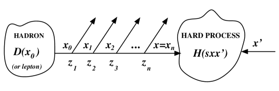
Figure 1: Graphical representation of the iterative series of eq. (8)

3.1 Solution types I and II

What are the general classes of the constrained MC solutions? Let us write once again the iterative solution of the evolution equations convoluted with the parton distribution $D_{k_{0}}(\tau_{0},x_{0})$ at the low energy scale $\tau_{0}$ and the hard-process matrix element denoted as $H(x)$ (see also fig. 1 for the illustration):

$$\begin{split}\sigma=&\sum_{k}\int dxH_{k}(x)D_{k}(\tau,x)\\ =&\sum_{k}\int dxH_{k}(x)\;\int_{0}^{1}dx_{0}\;\sum_{n=0}^{\infty}\;\sum_{k_{n-1}...k_{1}k_{0}}\bigg{[}\prod_{i=1}^{n}\;\;\int\limits_{\tau_{i-1}}^{\tau}d\tau_{i}\;\int\limits_{0}^{1}dz_{i}\;\bigg{]}\\ &~{}~{}\times e^{-(\tau-\tau_{n})R_{k}}\bigg{[}\prod_{i=1}^{n}\mathcal{P}_{k_{i}k_{i-1}}^{\Theta}(z_{i})\;e^{-(\tau_{i}-\tau_{i-1})R_{k_{i-1}}}\bigg{]}\;\delta\bigg{(}x-x_{0}\prod_{i=1}^{n}z_{i}\bigg{)}\;D_{k_{0}}(\tau_{0},x_{0}),\end{split}$$ (8)

where we define $k\equiv k_{n}$ and $\prod\limits_{k=1}^{0}\equiv 1$ in order to keep the formula compact. In the LL kernels and form factors simplify and from eq. (3) it follows that:

$$\Phi_{k}(\tau,\tau_{0})=(\tau-\tau_{0})R_{k},\qquad R_{k}\equiv\mathcal{P}_{kk}^{\delta}(\varepsilon)=\sum_{j}\int_{0}^{1-\epsilon}dz\;z\mathcal{P}^{\Theta}_{jk}(z).$$ (9)

For the purpose of future discussion we define here additional virtual form factors:

$$R_{jk}=\int_{0}^{1-\epsilon}dz\;z\mathcal{P}^{\Theta}_{jk}(z),\quad R_{k}^{\prime}=\sum_{j\neq k}R_{jk}=R_{k}-R_{kk}.$$ (10)

Let us discuss basic limitations and possible solutions for the MC implementation of the above series of multidimensional integrals. As already stated, in the ISR case, since there are narrow resonances in the hard-process function $H(x)$, the variable $x$ has to be the first one generated in the MC algorithm, i.e. it has to be the outermost integration variable. Similarly it is better to keep $k=k_{n}$ as the outermost summation variable as well.

The central issue is the following: How do we treat the variable $x_{0}$? There are two possible options. In the first option (I) $x_{0}$ is kept as a second outermost integration variable, next to $x$, i.e. it is generated in the MC as a second variable. In the second option (II) $x_{0}$ is treated as one of the last variables in the MC – in fact it is derived from the other ones using energy constraint.

The following formula describes the first case:

$$\begin{split}&\sigma=\sum_{kk_{0}}\int\frac{dx_{0}}{x_{0}}\int dx\;H_{k}(x)\;\mathcal{D}_{kk_{0}}\Bigl{(}\tau,\frac{x}{x_{0}}\Big{|}\tau_{0}\Bigr{)}\;D_{k_{0}}(\tau_{0},x_{0}),\\ &\mathcal{D}_{kk_{0}}(\tau,z|\tau_{0})=\sum_{n=0}^{\infty}\;\sum_{k_{n-1}...k_{1}}\bigg{[}\prod_{i=1}^{n}\;\;\int\limits_{\tau_{i-1}}^{\tau}d\tau_{i}\;\int\limits_{0}^{1}dz_{i}\;\bigg{]}\\ &~{}~{}~{}~{}~{}~{}\times e^{-(\tau-\tau_{n})R_{k}}\bigg{[}\prod_{i=1}^{n}\mathcal{P}_{k_{i}k_{i-1}}^{\Theta}(z_{i})\;e^{-(\tau_{i}-\tau_{i-1})R_{k_{i-1}}}\bigg{]}\;\delta\bigg{(}z-\prod_{i=1}^{n}z_{i}\bigg{)},\end{split}$$ (11)

with $k\equiv k_{n}$ as usual. We shall refer to this option as to a solution type I; this is the scenario that was implemented for the QED ISR pure bremsstrahlung in several YFS-type MC programs, starting from the prototype of ref. [13]. The main technical difficulty is the implementation/elimination of the $\delta(z-\prod z_{i})$ function. This problem was solved in QED by eliminating the delta function with integration over the $z$ of the hardest photon (the largest $1-z$). This scenario looks definitely feasible, and the first working example will be described in a separate work; see ref. [10].

The second scenario, referred to as solution type II relies on the fact that the starting parton distribution for typical hadron beam particle $D_{k_{0}}(\tau_{0},x)$ can be relatively well (by MC standards) approximated by a power-like function $D_{k_{0}}(\tau_{0},x)\sim x^{-1+\eta}$ over a wide range of $\ln(x)$ (i.e. $10^{-4}<x<1$), with the parameter $\eta$ not far from zero. In fact the gluon and quark singlet parton distributions of the nucleon at low $Q$ feature $\eta\simeq-0.2$. In solutions of type II the essential idea is that, in eq. (8), the $\delta\big{(}x-x_{0}\prod_{i=1}^{n}z_{i}\big{)}$ is eliminated using the integration over $x_{0}$. It means that $x_{0}$, contrary to type I, is generated in the MC as a last variable instead of a second one. More precisely it is not generated at all, but determined as a function of all previously generated variables $x_{0}=x\bigl{(}\prod z_{i}\bigr{)}^{-1}$, by means of solving the energy constraint.

Let us isolate explicitly the small-$z$ limit from the starting parton distribution:

$$D_{k_{0}}(\tau_{0},x_{0})=W^{*D}_{k_{0}}(x_{0})\;A_{k_{0}}x_{0}^{-1+\eta},\qquad W^{*D}_{k_{0}}(x_{0})\equiv\frac{D_{k_{0}}(\tau_{0},x_{0})}{A_{k_{0}}x_{0}^{-1+\eta}}\leq 1,$$ (12)

where $W^{*D}_{k}$ is the MC weight to be neglected now and restored later on. Elimination of the $\delta$-functions with the help of the $x_{0}$-integration leads to

$$\begin{split}\sigma=&\sum_{k}\int dx\;H_{k}(x)\;A_{k_{0}}x^{-1+\eta}\;\sum_{n=0}^{\infty}\;\sum_{k_{n-1}...k_{1}k_{0}}\bigg{[}\prod_{i=1}^{n}\;\;\int\limits_{\tau_{i-1}}^{\tau}d\tau_{i}\;\int\limits_{0}^{1}dz_{i}\;\bigg{]}\\ &~{}~{}\times e^{-(\tau-\tau_{n})R_{k}}\bigg{[}\prod_{i=1}^{n}z_{i}^{-\eta}\mathcal{P}_{k_{i}k_{i-1}}^{\Theta}(z_{i})\;e^{-(\tau_{i}-\tau_{i-1})R_{k_{i-1}}}\bigg{]}\;\Theta\Big{(}\prod_{j=1}^{n}z_{j}-x\Big{)}W^{*D}_{k_{0}}(\bar{x}_{0}),\end{split}$$ (13)

where $\bar{x}_{0}=x/\prod_{j}z_{j}$. For the distributions of quarks and gluons in the proton at a low energy scale we have the same $\eta\simeq-0.2$. Hence, we may also include all factors $z_{i}^{-\eta}$ in the MC weight $W^{D}_{k}\leq 1$, to be neglected and restored at a later stage of the MC algorithm together with the other details of the $D_{k}(\tau_{0},x_{0})$ function, or in a more sophisticated MC algorithm, we may actually generate exactly the distributions $z_{i}^{-\eta}\mathcal{P}_{k_{i}k_{i-1}}^{\Theta}(z_{i})$. In the following let us assume the former simpler case with $z_{i}^{-\eta}$ in the MC weight:

$$\begin{split}&\sigma=\sum_{k}\int dx\;H_{k}(x)\;A_{k_{0}}x^{-1+\eta}\;\sum_{n=0}^{\infty}\;\sum_{k_{n-1}...k_{1}k_{0}}\bigg{[}\prod_{i=1}^{n}\;\;\int\limits_{\tau_{i-1}}^{\tau}d\tau_{i}\;\int\limits_{0}^{1}dz_{i}\;\bigg{]}\\ &~{}~{}~{}~{}~{}~{}~{}\times e^{-(\tau-\tau_{n})R_{k}}\bigg{[}\prod_{i=1}^{n}\mathcal{P}_{k_{i}k_{i-1}}^{\Theta}(z_{i})\;e^{-(\tau_{i}-\tau_{i-1})R_{k_{i-1}}}\bigg{]}\;\Theta\Big{(}\prod_{j=1}^{n}z_{j}-x\Big{)}W^{D}_{k}(x,\bar{x}_{0}),\\ &W^{D}_{k_{0}}(x,\bar{x}_{0})=\frac{D_{k_{0}}(\tau_{0},\bar{x}_{0})}{A_{k_{0}}\bar{x}_{0}^{-1+\eta}}\bigg{\{}\prod_{i=1}^{n}z_{i}\bigg{\}}^{-\eta}=\frac{D_{k_{0}}(\tau_{0},\bar{x}_{0})}{A_{k_{0}}\bar{x}_{0}^{-1+\eta}}\bigg{\{}\frac{x}{\bar{x}_{0}}\bigg{\}}^{-\eta}\leq 1,\end{split}$$ (14)

where $D_{k_{0}}(\tau_{0},\bar{x}_{0})\to A_{k_{0}}\bar{x}_{0}^{-1+\eta}$ in the limit $\bar{x}_{0}\to 0$.

Let us stress that eq. (13) implements the exact iterative distribution of the evolution equations. In the following sections we will show the results from the prototype MC based directly on the above expression for the pure bremsstrahlung case. As we shall see, it works well for the case of the emission from a quark; however, it has rather low acceptance ($\sim 10^{-3}$) for the emission from a gluon. We shall call such a MC solution, directly based on eq. (13), solution type II.a.

In another method, II.b, we shall reorganize the integration variables in a hierarchical way, and use multibranching to isolate the $1/z$ part of the gluon-to-gluon kernel. Such a solution is rather complicated and non-trivial to implement in a general case with multiple flavour-changing (quark–gluon) transitions. However, successful implementation of the pure gluon-strahlung case, presented in the next section, allows us to claim that the efficiency of the MC type II.b is satisfactory, and the gate to practical applications of MC solutions of this type is wide open.

3.2 Constrained Monte Carlo: solutions class II

As already noticed in ref. [8], in the long emission chain (on average $\sim 20$ emissions), from $Q=1$ GeV to $Q=1$ TeV, most of the emissions are of bremsstrahlung type, i.e. they preserve the identity of the parton on the main line of the chain. It was shown there that on the average only about one out of twenty emissions involves flavour transmutation, $q\to G$ or $G\to q$; the other ones are gluon emissions. With this in mind, it is therefore natural to reorganize the iterative solution of the evolution equations in such a way that all pure bremsstrahlung adjacent vertices in the emission chain are lumped together into segments described by the following universal evolution function:

$$\begin{split}d^{\prime}_{k}(\tau,z|\tau_{0})=&e^{-(\tau-\tau_{0})R_{kk}}\sum_{n=0}^{\infty}\;\prod_{i=1}^{n}\;\int\limits_{\tau_{i-1}}^{\tau}d\tau_{i}\;\int\limits_{0}^{1}dz_{i}\;\mathcal{P}_{kk}^{\Theta}(z_{i})\;\delta\bigg{(}z-\prod_{j=1}^{n}z_{j}\bigg{)},\end{split}$$ (15)

where the type of parton on the main line, $k=Q$ or $k=G$, is unchanged. Note that we have retained in eq. (15) only part of the virtual form factor $R_{k}$, namely the $R_{kk}$ function, which matches exactly the real emission kernel $\mathcal{P}_{kk}^{\Theta}$ of pure bremsstrahlung. The leftover $R^{\prime}_{k}$ is included explicitly in the following eq. (16).

The full iterative solution of the previous section can be expressed in terms of the product of the above functions and the kernels representing flavour-changing transitions $q\to G$ or $G\to q$ in the following way:

$$\begin{split}D_{k}(\tau,x)&=\sum_{n=0}^{\infty}\;\int\limits_{0}^{1}dx_{0}\;\sum_{{k_{n-1}\dots,k_{1},k_{0}}\atop{k_{j}\neq k_{j-1},j=1,\dots,n}}\Biggl{(}\prod_{i=1}^{n}\;\int\limits_{\tau_{i-1}}^{\tau}d\tau_{i}\Biggr{)}\Biggl{(}\prod_{i=1}^{n}\int\limits_{0}^{1}dz_{i}\Biggr{)}\Biggl{(}\prod_{i=1}^{n+1}\int\limits_{0}^{1}dz^{\prime}_{i}\Biggr{)}\\ &~{}~{}~{}\times e^{-(\tau-\tau_{n})R^{\prime}_{k}}\;d^{\prime}_{k}(\tau,z^{\prime}_{n+1}|\tau_{n})\;\\ &~{}~{}~{}\times\prod_{i=1}^{n}\bigg{[}\mathcal{P}_{k_{i}k_{i-1}}^{\Theta}(z_{i})\;e^{-(\tau_{i}-\tau_{i-1})R^{\prime}_{k_{i-1}}}\;d^{\prime}_{k_{i-1}}(\tau_{i},z^{\prime}_{i}|\tau_{i-1})\bigg{]}\;\\ &~{}~{}~{}\times D_{k_{0}}(\tau_{0},x_{0})\delta\bigg{(}x-x_{0}\prod_{i=1}^{n}z_{i}\prod_{i=1}^{n+1}z^{\prime}_{i}\bigg{)},\end{split}$$ (16)

where we employ the usual conventions: $k_{n}\equiv k$ and $\prod_{j=1}^{0}\equiv 1$.

We say that the above formula implements hierarchical organization of the emission chain, because it represents the Markovian process in which each pure bremsstrahlung step (segment) in the Markovian random walk (emission chain) is an independent Markovian process of its own! This elegant and powerful reorganization of the emission chain is proved formally in the separate work of ref. [14].

The complete hierarchical formula for the integrated cross section, after elimination of the delta function with $x_{0}$ integration, reads as follows:

$$\begin{split}\sigma=\sum_{k}\int dx\;&H_{k}(x)\;A_{k_{0}}x^{-1+\eta}\;\sum_{n=0}^{\infty}\;\sum_{{k_{n-1}\dots,k_{1},k_{0}}\atop{k_{j}\neq k_{j-1},j=1,\dots,n}}\prod_{i=1}^{n}\;\int\limits_{\tau_{i-1}}^{\tau}d\tau_{i}\;\prod_{i=1}^{n}\int\limits_{0}^{1}dz_{i}\;\prod_{i=1}^{n+1}\int\limits_{0}^{1}dz^{\prime}_{i}\;\\ &~{}~{}~{}\times e^{-(\tau-\tau_{n})R^{\prime}_{k}}\;d^{\prime}_{k}(\tau,z^{\prime}_{n+1}|\tau_{n})\;\\ &~{}~{}~{}\times\prod_{i=1}^{n}\bigg{[}\mathcal{P}_{k_{i}k_{i-1}}^{\Theta}(z_{i})\;e^{-(\tau_{i}-\tau_{i-1})R^{\prime}_{k_{i-1}}}\;d^{\prime}_{k_{i-1}}(\tau_{i},z^{\prime}_{i}|\tau_{i-1})\bigg{]}\;\\ &~{}~{}~{}\times\Theta\bigg{(}\prod_{i=1}^{n}z_{i}\prod_{i=1}^{n+1}z^{\prime}_{i}-x\bigg{)}W^{D}_{k_{0}}(x,\bar{x}_{0}),\\ d^{\prime}_{k}(\tau_{i},z^{\prime}_{i}|\tau_{i-1})=&e^{-(\tau_{i}-\tau_{i-1})R_{kk}}\sum_{n^{(i)}=0}^{\infty}\;\prod_{m=1}^{n^{(i)}}\;\int\limits_{\tau^{(i)}_{m-1}}^{\tau^{(i)}}d\tau^{(i)}_{m}\;\int\limits_{0}^{1}dz^{(i)}_{m}\;\mathcal{P}_{kk}^{\Theta}(z^{(i)}_{m})\;\delta\bigg{(}z^{\prime}_{i}-\prod_{m=1}^{n^{(i)}}z^{(i)}_{m}\bigg{)}.\end{split}$$ (17)

where

$$\tau^{(i)}\equiv\tau_{i},\quad\tau^{(i)}_{0}\equiv\tau_{i-1},\quad\bar{x}_{0}=\frac{x}{\prod_{i=1}^{n}z_{i}\prod_{i=1}^{n+1}z^{\prime}_{i}}\leq 1.$$ (18)

The above formula is the starting point in the next two subsections for construction of constrained MC algorithms of type II.

3.2.1 Solution II.a

In the straightforward solution of type II, which we call II.a, the single $\Theta$-function for both flavour-changing emissions and pure bremsstrahlung segments is replaced by the product of the individual $\Theta$-functions – thus decoupling completely the $z$-integration space and opening the way for the analytical integrations of the approximate spectra for the purpose of the MC generation. More precisely, let us first notice that we are really dealing with the single $\Theta$-function involving all $z$ variables due to trivial identity

$$\begin{split}\prod_{i=1}^{n+1}\Biggl{[}\int\limits_{0}^{1}dz^{\prime}_{i}\;\biggl{(}\prod_{m=1}^{n^{(i)}}\;\int\limits_{0}^{1}dz^{(i)}_{m}\;\biggr{)}\delta\bigg{(}z^{\prime}_{i}-\prod_{m=1}^{n^{(i)}}z^{(i)}_{m}\bigg{)}\Biggr{]}&\Theta\bigg{(}\prod_{i=1}^{n}z_{i}\prod_{i=1}^{n+1}z^{\prime}_{i}-x\bigg{)}=\\ =\prod_{i=1}^{n+1}\biggl{(}\prod_{m=1}^{n^{(i)}}\;\int\limits_{0}^{1}dz^{(i)}_{m}\;\biggr{)}&\Theta\bigg{(}\prod_{i=1}^{n}z_{i}\prod_{i=1}^{n+1}\prod_{m=1}^{n^{(i)}}z^{(i)}_{m}-x\bigg{)}.\end{split}$$ (19)

We are now ready to describe the essence of the MC algorithm of type II.a. We use the following identity

$$\begin{split}&\Theta\bigg{(}\prod_{i=1}^{n}z_{i}\prod_{i=1}^{n+1}\prod_{m=1}^{n^{(i)}}z^{(i)}_{m}-x\bigg{)}=W^{\Theta}_{II.a}\;\;\prod_{i=1}^{n}\Theta(z_{i}-x)\prod_{i=1}^{n+1}\prod_{m=1}^{n^{(i)}}\Theta\bigg{(}z^{(i)}_{m}-x\bigg{)},\end{split}$$ (20)

where the function

$$\begin{split}&W^{\Theta}_{II.a}\equiv\Theta\left(\prod_{i=1}^{n}z_{i}\prod_{i=1}^{n+1}\prod_{m=1}^{n^{(i)}}z^{(i)}_{m}-x\right)\leq 1\end{split}$$ (21)

is the Monte Carlo weight. This MC weight will be neglected later on, so that variables can be generated according to simplified distributions, and finally the generated events will be weighted according to this weight.

Let us rewrite our master integral (17) without any approximations

$$\begin{split}\sigma&=\sum_{k}\int dx\;H_{k}(x)\;A_{k_{0}}x^{-1+\eta}\;\sum_{n=0}^{\infty}\;\sum_{{k_{n-1}\dots,k_{1},k_{0}}\atop{k_{j}\neq k_{j-1},j=1,\dots,n}}\bigg{[}\prod_{i=1}^{n}\;\int\limits_{\tau_{i-1}}^{\tau}d\tau_{i}\;\int\limits_{x}^{1}dz_{i}\;\bigg{]}\\ &\times e^{-(\tau-\tau_{n})R^{\prime}_{k}}d^{\prime\prime}_{k}(\tau,x|\tau_{n})\bigg{[}\prod_{i=1}^{n}\mathcal{P}_{k_{i}k_{i-1}}^{\Theta}(z_{i})e^{-(\tau_{i}-\tau_{i-1})R^{\prime}_{k_{i-1}}}d^{\prime\prime}_{k_{i-1}}(\tau_{i},x|\tau_{i-1})\bigg{]}W^{D}_{k_{0}}(x,\bar{x}_{0})W^{\Theta}_{\rm II.a},\\ d&{}^{\prime\prime}_{k}(\tau_{i},x|\tau_{i-1})=e^{-(\tau_{i}-\tau_{i-1})R_{kk}}\sum_{n^{(i)}=0}^{\infty}\;\prod_{m=1}^{n^{(i)}}\;\int\limits_{\tau^{(i)}_{m-1}}^{\tau^{(i)}}d\tau^{(i)}_{m}\;\prod_{m=1}^{n^{(i)}}\;\int\limits_{x}^{1}dz^{(i)}_{m}\;\mathcal{P}_{kk}^{\Theta}(z^{(i)}_{m})\end{split}$$ (22)

where $\bar{x}_{0}=x/\Big{(}\prod_{i=1}^{n}z_{i}\prod_{i=1}^{n+1}\prod_{m=1}^{n^{(i)}}z^{(i)}_{m}\Big{)}$ and one should remember that $d^{\prime\prime}$-functions provide integration over all the $z^{(i)}_{i}$ variables that are implicitly present in the function $W^{\Theta}_{\rm II.a}$. The enormous advantage of the above procedure is that in the approximate integral we can sum up and integrate immediately over all bremsstrahlung segments of the emission chain. To see it let us drop the two MC weights $W^{D}_{k_{0}}$ and $W^{\Theta}_{\rm II.a}$. Now we can immediately sum up and integrate analytically the pure bremsstrahlung subintegrals:

$$d^{\prime\prime}_{k}(\tau_{i},x|\tau_{i-1})=\exp\biggl{(}(\tau_{i}-\tau_{i-1})\Bigl{(}-R_{kk}+\int\limits_{x}^{1}dz\;\mathcal{P}_{kk}^{\Theta}(z)\Bigr{)}\biggr{)}$$ (23)

and hence

$$\begin{split}\sigma&=\sum_{k}\int dx\;H_{k}(x)\;A_{k_{0}}x^{-1+\eta}\;\sum_{n=0}^{\infty}\;\sum_{{k_{n-1}\dots,k_{1},k_{0}}\atop{k_{j}\neq k_{j-1},j=1,\dots,n}}\bigg{[}\prod_{i=1}^{n}\;\int\limits_{\tau_{i-1}}^{\tau}d\tau_{i}\;\int\limits_{x}^{1}dz_{i}\;\bigg{]}\\ &\times e^{(\tau-\tau_{n})(-R_{k}+\int_{x}^{1}dz\mathcal{P}_{kk}^{\Theta}(z))}\;\bigg{[}\prod_{i=1}^{n}\mathcal{P}_{k_{i}k_{i-1}}^{\Theta}(z_{i})\;e^{(\tau_{i}-\tau_{i-1})(-R_{k_{i-1}}+\int_{x}^{1}dz\mathcal{P}_{k_{i-1}k_{i-1}}^{\Theta}(z))}\bigg{]}.\end{split}$$ (24)

The above looks rather promising, because we are left with the relatively simple problem of generating several variables $\tau_{i}$ and $z_{i}$ ($i\leq 5$ seems sufficient) for the flavour-changing emissions, for which the above integrals provide explicit analytical distribution. The MC events are attributed with the MC weight $W_{\rm II.a}=W^{D}_{k_{0}}(\bar{x}_{0})\;W^{\Theta}_{\rm II.a}\leq 1$. The key question is: What is the acceptance rate for this weight? We did an introductory exercise, implementing the pure bremsstrahlung version of it. We have found that, unfortunately, the acceptance rate for the emission from the gluon line is only about $10^{-4}$. This inefficiency can be traced back to the presence of the $1/z$ singularity in the $G\to G$ kernel. Namely, if we allow for the range $x>x_{\min}=10^{-5}$ we also allow for $z$ to be generated to the same low limit. In the case of $\mathcal{P}_{GG}(z)$ containing a $1/z$ part, this creates many events with low $z_{i}$. Consequently, $\bar{x}_{0}=x/\prod z_{i}$ goes very often beyond 1 and the corresponding MC weight $W^{\Theta}_{\rm II.a}$ gets zero value.

On the other hand, for the quark line the acceptance rate is close to 1, which is clearly related to the absence of the component $1/z$ in $\mathcal{P}_{qq}(z)$.

The above numerical exercise indicates that the $1/z$ part in the $\mathcal{P}_{GG}(z)$ has to be treated better, as is done in the present case II.a. A more sophisticated treatment of the $1/z$ component of the kernel is applied in the solution II.b described in the next section.

The present solution II.a is still a workable solution. In spite of its very low efficiency, due to its relative simplicity, it can still be quite useful for testing other more sophisticated solutions. We therefore implemented it also in the MC program, for the moment only in the pure bremsstrahlung version.

3.2.2 Solution II.b

In this section we present a solution more sophisticated than the II.a one of the previous section: we split the bremsstrahlung kernel $\mathcal{P}_{GG}$ into two parts: (B) $\sim 1/z$ and (A) = the rest. Then we apply the multibranching, as described in Appendix A, to every pure bremsstrahlung segment of the emission chain. Finally, we also treat the $\Theta$-function more selectively than in II.a. The product of the individual $\Theta$-functions appears for the flavour-changing emissions and part (A) of the bremsstrahlung kernel, while the single $\Theta$-function is left for each segment describing part (B) of the pure bremsstrahlung. Such partial decoupling in the $z$-integration space still allows for the analytical integration of the approximate spectra for the purpose of the early stage of the MC generation. This is possible because segments of type (B) in the pure bremsstrahlung parts are integrable (to a Bessel function), as shown below, while for the rest we get exponentials in a way similar to those in II.a.

Again, the starting point is the complete hierarchical formula (17) for the integrated cross section. In the case of the gluonic subintegral $d^{\prime}_{k=G}(\tau_{i},z^{\prime}_{i}|\tau_{i-1})$ we reorganize this integral to isolate the $1/z$ part from the kernel. In order to split the $\mathcal{P}_{GG}(z)$ in two positive parts, one of them being $1/z$, we have to simplify it first:

$$\begin{split}&\mathcal{P}^{\Theta}_{GG}(z)=\bar{\mathcal{P}}^{\Theta}_{GG}(z)\;w_{GG}(z),\quad P^{\Theta}_{GG}(z)=\bar{P}^{\Theta}_{GG}(z)\;w_{GG}(z),\quad\\ &\bar{P}^{\Theta}_{GG}(z)=2C_{A}\left(\frac{1}{z}+\frac{1}{1-z}\right),\quad w_{GG}(z)=(1-z(1-z))^{2}\leq 1.\end{split}$$ (25)

Having done that and using the multibranching identity of eq. (91) in the appendix we may rewrite the gluonic bremsstrahlung subintegral for $k=G$ as follows:

$$\begin{split}&d^{\prime}_{k}(\tau_{i},z^{\prime}_{i}|\tau_{i-1})=\int\limits_{0}^{1}\frac{dZ^{(i)}}{Z^{(i)}}\;\Theta(Z^{(i)}-z^{\prime}_{i})d^{B}_{k}(\tau_{i},Z^{(i)}|\tau_{i-1})\,d^{A}_{k}\biggl{(}\tau_{i},\frac{z^{\prime}_{i}}{Z^{(i)}}|\tau_{i-1}\biggr{)}W_{kk}\bigl{(}{\bf z^{(i)}}({\bf z^{\bullet(i)},{z^{\prime}}^{(i)}})\bigr{)},\end{split}$$ (26)

where

$$\begin{split}&d^{A}_{k}(\tau_{i},Z^{(i)}|\tau_{i-1})=e^{-(\tau_{i}-\tau_{i-1})R^{A}_{kk}}\\ &~{}~{}\times\sum_{n^{\prime(i)}=0}^{\infty}\;\;\prod_{m=1}^{n^{\prime(i)}}\int\limits^{\tau_{i}}_{\tau_{i-1}}d\tau^{\prime(i)}_{m}\;\Theta(\tau^{\prime(i)}_{m}-\tau^{\prime(i)}_{m-1})\prod_{m=1}^{n^{\prime(i)}}\int dz_{m}^{\prime(i)}\;\bar{\mathcal{P}}_{kk}^{\Theta A}(z_{m}^{\prime(i)})\;\delta\bigg{(}Z^{(i)}-\prod_{m=1}^{n^{\prime(i)}}z_{m}^{\prime(i)}\bigg{)}\\ &d^{B}_{k}(\tau_{i},Z^{(i)}|\tau_{i-1})=e^{-(\tau_{i}-\tau_{i-1})R^{B}_{kk}}\\ &~{}~{}\times\sum_{n^{\bullet(i)}=0}^{\infty}\;\;\prod_{m=1}^{n^{\bullet(i)}}\int\limits^{\tau_{i}}_{\tau_{i-1}}d\tau^{\bullet(i)}_{m}\;\Theta(\tau^{\bullet(i)}_{m}-\tau^{\bullet(i)}_{m-1})\prod_{m=1}^{n^{\bullet(i)}}\int dz_{m}^{\bullet(i)}\;\bar{\mathcal{P}}_{kk}^{\Theta B}(z_{m}^{\bullet(i)})\;\delta\bigg{(}Z^{(i)}-\prod_{m=1}^{n^{\bullet(i)}}z_{m}^{\bullet(i)}\bigg{)}\end{split}$$ (27)

and

$$\begin{split}&\bar{P}^{\Theta A}_{GG}(z)=\frac{2C_{A}}{1-z},\qquad\bar{P}^{\Theta B}_{GG}(z)=\frac{2C_{A}}{z},\Biggl{.}\\ &\mathcal{P}^{\Theta B}_{GG}(z)=\bar{\mathcal{P}}^{\Theta B}_{GG}(z),\qquad\mathcal{P}^{\Theta A}_{GG}(z)=\mathcal{P}^{\Theta}_{GG}(z)-\mathcal{P}^{\Theta B}_{GG}(z).\end{split}$$ (28)

In the above we used the notation ${\bf{z^{\prime}}^{(i)}}=\bigl{(}{z^{\prime}}^{(i)}_{1},\dots,{z^{\prime}}^{(i)}_{n^{\prime(i)}}\bigr{)}$ and ${\bf z^{\bullet(i)}}=\bigl{(}{z}^{\bullet(i)}_{1},\dots,{z}^{\bullet(i)}_{n^{\bullet(i)}}\bigr{)}$.

The MC weight due to the kernel simplification

$$W_{GG}\bigl{(}{\bf z^{(i)}}({\bf z^{\bullet(i)},{z^{\prime}}^{(i)}})\bigr{)}=\prod_{m=1}^{n^{\bullet(i)}+{n^{\prime}}^{(i)}}w_{GG}\bigl{(}z^{(i)}_{m}({\bf z^{\bullet(i)},{z^{\prime}}^{(i)}})\bigr{)},$$ (29)

depends on the variables $z^{(i)}_{m}$ after relabelling. A special kind of permutation $z^{(i)}_{m}\to z^{\bullet(i)}_{l},{z^{\prime}}^{(i)}_{l}$, which we refer to as relabelling, is an important part of the MC algorithm – it is defined precisely in the appendix. Since relabelling is just a permutation of $z$’s, we may calculate the weight $W_{GG}$ with the $z^{\bullet(i)}_{l},{z^{\prime}}^{(i)}_{l}$ variables before the relabelling:

$$W_{GG}=\prod_{m=1}^{n^{\bullet(i)}}w_{GG}(z^{\bullet(i)}_{m})\;\;\prod_{m=1}^{{n^{\prime}}^{(i)}}w_{GG}({z^{\prime}}^{(i)}_{m}).$$ (30)

Until now we made no approximation in our master integral – we only reorganized integration variables, in particular isolating the $1/z$ component in the pure bremsstrahlung subintegrals for the gluon emitters. In full analogy to case II.a, in the last step in this reorganization we eliminate all variables $z^{\prime}_{i}$ and a class of $\delta$-functions with the help of the identity:

$$\begin{split}\prod_{i=1}^{n+1}\int\limits_{0}^{1}dz^{\prime}_{i}\;\Theta(Z^{(i)}-z^{\prime}_{i})\;&\prod_{i=1}^{n+1}\delta\bigg{(}\frac{z^{\prime}_{i}}{Z^{(i)}}-\prod_{m=1}^{{n^{\prime}}^{(i)}}{z^{\prime}}^{(i)}_{m}\bigg{)}~{}\Theta\bigg{(}\prod_{i=1}^{n}z_{i}\prod_{i=1}^{n+1}z^{\prime}_{i}-x\bigg{)}=\\ =&\prod_{i=1}^{n+1}Z^{(i)}\;\Theta\Bigg{(}\prod_{i=1}^{n}z_{i}\prod_{i=1}^{n+1}\bigg{(}Z^{(i)}\prod_{m=1}^{{n^{\prime}}^{(i)}}{z^{\prime}}^{(i)}_{m}\bigg{)}-x\Bigg{)}.\end{split}$$ (31)

Consequently, from now on we substitute $z^{\prime}_{i}$ with $\bar{z}^{\prime}_{i}$

$$z^{\prime}_{i}\to\bar{z}^{\prime}_{i}=Z^{(i)}\prod_{m=1}^{{n^{\prime}}^{(i)}}{z^{\prime}}^{(i)}_{m}\leq 1.$$ (32)

On the other hand, we keep $\delta$-functions inside the $d_{G}^{B}$ functions, which will also be treated analytically, but separately; see below.

Now comes the essential step in the algorithm II.b – we define the following MC weight:

$$\begin{split}&\Theta\bigg{(}\bigg{\{}\prod_{j=1}^{n}z_{j}\prod_{j=1}^{n+1}\;Z^{(j)}\bigg{\}}\bigg{\{}\prod_{i=1}^{n+1}\;\prod_{m=1}^{{n^{\prime}}^{(i)}}{z^{\prime}}^{(i)}_{m}\bigg{\}}-x\bigg{)}=\\ &~{}~{}~{}~{}~{}~{}~{}~{}~{}~{}~{}~{}~{}~{}~{}~{}~{}=W^{\Theta}_{\rm II.b}~{}\Theta\bigg{(}\prod_{j=1}^{n}z_{j}\prod_{j=1}^{n+1}\;Z^{(j)}-x\bigg{)}\prod_{i=1}^{n+1}\prod_{m=1}^{{n^{\prime}}^{(i)}}\Theta\bigg{(}\bigg{\{}\prod_{j=1}^{n}z_{j}\prod_{j=1}^{n+1}\;Z^{(j)}\bigg{\}}{z^{\prime}}^{(i)}_{m}-x\bigg{)}\\ &~{}~{}~{}~{}~{}~{}~{}~{}~{}~{}~{}~{}~{}~{}~{}~{}~{}=W^{\Theta}_{\rm II.b}~{}\Theta\Big{(}1-z^{\rm eff}_{\min}({\bf z},{\bf Z})\Big{)}\prod_{i=1}^{n+1}\prod_{m=1}^{{n^{\prime}}^{(i)}}\Theta\Big{(}{z^{\prime}}^{(i)}_{m}-z^{\rm eff}_{\min}({\bf z},{\bf Z})\Big{)},\end{split}$$ (33)

where

$$z^{\rm eff}_{\min}\Big{(}z_{1},z_{2},...,z_{n},Z^{(1)},Z^{(2)},...,Z^{(n+1)}\Big{)}\;\equiv\;\frac{x}{\prod_{j=1}^{n}z_{j}\prod_{j=1}^{n+1}\;Z^{(j)}}.$$ (34)

The new MC weight

$$\begin{split}&W^{\Theta}_{\rm II.b}\equiv\Theta\left(\prod_{i=1}^{n}z_{i}\prod_{i=1}^{n+1}\biggl{(}Z^{(i)}\prod_{m=1}^{{n^{\prime}}^{(i)}}z^{(i)}_{m}\biggr{)}-x\right)\leq 1\end{split}$$ (35)

will be neglected later on and restored at the end as a standard MC compensating weight.

All these preparatory steps lead us to the following master equation for method II.b, still without any approximation, but with clearly defined MC weights and the distributions to be generated at the early stage of the MC algorithm:

$$\begin{split}\sigma=\sum_{k}\int dx\;&H_{k}(x)\;A_{k_{0}}x^{-1+\eta}\;\sum_{n=0}^{\infty}\;\sum_{{k_{n-1}\dots,k_{1},k_{0}}\atop{k_{j}\neq k_{j-1},j=1,\dots,n}}\prod_{i=1}^{n}\;\int\limits_{\tau_{i-1}}^{\tau}d\tau_{i}\;\prod_{i=1}^{n}\int\limits_{0}^{1}dz_{i}\;\prod_{i=1}^{n+1}\int\limits_{0}^{1}\frac{dZ^{(i)}}{Z^{(i)}}\;\\ &\times e^{-(\tau-\tau_{n})R^{\prime}_{k}}\;{d^{A}_{k}}^{\prime}(\tau,z^{\rm eff}_{\min}|\tau_{n})\;d^{B}_{k}(\tau,Z^{(n+1)}|\tau_{n})\\ &\times\prod_{i=1}^{n}\bigg{[}\mathcal{P}_{k_{i}k_{i-1}}^{\Theta}(z_{i})\;e^{-(\tau_{i}-\tau_{i-1})R^{\prime}_{k_{i-1}}}\;{d^{A}_{k_{i-1}}\hskip-8.53581pt}^{\prime}\hskip 8.53581pt(\tau_{i},z^{\rm eff}_{\min}|\tau_{i-1})\;d^{B}_{k}(\tau_{i},Z^{(i)}|\tau_{i-1})\bigg{]}\;\;\\ &\times W^{D}_{k_{0}}(\bar{x}_{0})\;W^{\Theta}_{\rm II.b}\;{\Theta(1-z^{\rm eff}_{\min})},\\ {d^{A}_{k}}^{\prime}(\tau_{i},z^{\rm eff}_{\min}|\tau_{i-1})&=e^{-(\tau_{i}-\tau_{i-1})R^{A}_{kk}}\sum_{n^{\prime(i)}=0}^{\infty}\;\prod_{m=1}^{n^{\prime(i)}}\;\int\limits_{\tau^{\prime(i)}_{m-1}}^{\tau_{i}}d\tau^{\prime(i)}_{m}\;\\ &\times\prod_{m=1}^{n^{\prime(i)}}\;\int\limits_{0}^{1}dz^{\prime(i)}_{m}\;\bar{\mathcal{P}}_{kk}^{\Theta A}(z^{\prime(i)}_{m})\;\Theta\big{(}z^{\prime(i)}_{m}-z^{\rm eff}_{\min}\big{)}~{}W_{GG}({\bf z^{\bullet{(i)}}},{\bf{z^{\prime}}^{(i)}}).\end{split}$$ (36)

The functions $d^{B}_{k}(\tau_{i},Z^{(i)}|\tau_{i-1})$ and the variables $Z^{(i)}$ are really present only for gluon, $k=G$. However, in order to keep the notation compact, we understand that

$$d^{B}_{k\neq G}(\tau_{i},Z^{(i)}|\tau_{i-1})\equiv\delta(1-Z^{(i)}).$$ (37)

We also assume $\prod_{n=1}^{0}=1$, as usual. The reader should also keep in mind that at this stage the integrand of the part ${d^{A}}^{\prime}$ still depends on the integration variables of $d^{B}_{G}$.

In the MC algorithm of type II.b all three MC weights are neglected:

$$W^{D}_{k_{0}}(\bar{x}_{0})\;W^{\Theta}_{\rm II.b},W_{GG}({\bf z^{\bullet{(i)}}},{\bf{z^{\prime}}^{(i)}})\equiv W_{\rm II.b}$$ (38)

at the early stage of the MC algorithm and later on generated MC events are weighted with $W_{\rm II.b}$. Since $W_{\rm II.b}\leq 1$, we may easily transform weighted MC events into unweighted events by rejecting some of the MC events in the usual way.

The MC weight $W_{\rm II.b}$ was chosen in such a way that once it is neglected, we can perform a lot of analytical integrations:

$$\begin{split}\sigma_{\hbox{\footnotesize prim.}}=\sum_{k}\int&dx\;H_{k}(x)\;A_{k_{0}}x^{-1+\eta}\;\sum_{n=0}^{\infty}\;\sum_{{k_{n-1}\dots,k_{1},k_{0}}\atop{k_{j}\neq k_{j-1},j=1,\dots,n}}\prod_{i=1}^{n}\;\int\limits_{\tau_{i-1}}^{\tau}d\tau_{i}\;\prod_{i=1}^{n}\int\limits_{x}^{1}dz_{i}\;\prod_{i=1}^{n+1}\int\limits_{x}^{1}dZ^{(i)}\;\\ \times&e^{-(\tau-\tau_{n})R^{\prime}_{k}}\;{d^{A}_{k}}^{*}(\tau,z^{\rm eff}_{\min}|\tau_{n})\;\frac{1}{Z^{(n+1)}}d^{B}_{k}(\tau,Z^{(n+1)}|\tau_{n})\\ \times&\prod_{i=1}^{n}\bigg{[}\mathcal{P}_{k_{i}k_{i-1}}^{\Theta}(z_{i})\;e^{-(\tau_{i}-\tau_{i-1})R^{\prime}_{k_{i-1}}}\;{d^{A}_{k_{i-1}}\hskip-8.53581pt}^{*}\hskip 8.53581pt(\tau_{i},z^{\rm eff}_{\min}|\tau_{i-1})\;\frac{1}{Z^{(i)}}d^{B}_{k}(\tau_{i},Z^{(i)}|\tau_{i-1})\bigg{]}\;\;\\ \times&\Theta\bigg{(}\prod_{j=1}^{n}z_{j}\prod_{j=1}^{n+1}Z^{(j)}-x\bigg{)},\\ {d^{A}_{k}}^{*}(\tau_{i},z^{\rm eff}_{\min}|\tau_{i-1})&=e^{-(\tau_{i}-\tau_{i-1})R^{A}_{kk}}\sum_{n^{\prime(i)}=0}^{\infty}\;\prod_{m=1}^{n^{\prime(i)}}\;\int\limits_{\tau^{\prime(i)}_{m-1}}^{\tau_{i}}d\tau^{\prime(i)}_{m}\;\prod_{m=1}^{n^{\prime(i)}}\;\int\limits^{1}_{z^{\rm eff}_{\min}}dz^{\prime(i)}_{m}\;\bar{\mathcal{P}}_{kk}^{\Theta A}(z^{\prime(i)}_{m})\;\\ &=\exp\Biggl{(}{(\tau_{i}-\tau_{i-1})\biggl{(}-R^{A}_{kk}+\int\limits^{1}_{z^{\rm eff}_{\min}}dz\bar{\mathcal{P}}_{kk}^{\Theta A}(z)\biggr{)}}\Biggr{)},\;\;\;\tau^{(i)}_{0}=\tau_{i-1},\\ d^{B}_{G}(\tau_{i},Z^{(i)}|\tau_{i-1})&=e^{-(\tau_{i}-\tau_{i-1})R^{B}_{GG}}\bigg{\{}\delta(Z^{(i)}-1)+\\ &+\sum^{\infty}_{n^{\bullet(i)}=1}\;\;\frac{(\tau_{i}-\tau_{i-1})^{n^{\bullet(i)}}}{n^{\bullet(i)}!}\prod_{m=1}^{n^{\bullet(i)}}\int\limits_{0}^{1}dz_{m}^{\bullet(i)}\;\bar{\mathcal{P}}_{GG}^{\Theta B}(z_{m}^{\bullet(i)})\;\delta\Big{(}Z^{(i)}-\prod_{m=1}^{n^{\bullet(i)}}z_{m}^{\bullet(i)}\Big{)}\bigg{\}}.\end{split}$$ (39)

The distribution $d^{B}_{G}$ for the trouble-making component of the kernel $\bar{P}_{GG}^{\Theta B}(z)=P_{GG}^{\Theta B}(z)=2C_{A}/z$ and $R^{B}_{GG}=(\alpha_{S}(t_{A})/\pi)2C_{A}$, can be calculated analytically:

$$\begin{split}d^{B}_{G}(\tau_{i},Z^{(i)}|\tau_{i-1})=&e^{-(\tau_{i}-\tau_{i-1})R^{B}_{GG}}\Bigg{[}\delta(Z^{(i)}-1)\\ &+\frac{1}{Z^{(i)}}\sum_{n=1}^{\infty}\frac{(\tau_{i}-\tau_{i-1})^{n}}{n!}(R^{B}_{GG})^{n}\;\prod_{i=1}^{n}\int_{0}^{1}dz_{i}\;\delta\bigg{(}Z^{(i)}-\prod_{j=1}^{n}z_{j}\bigg{)}\Bigg{]}.\end{split}$$ (40)

The integral

$$\prod_{i=1}^{n}\int_{0}^{1}dz_{i}\;\delta\bigg{(}Z^{(i)}-\prod_{j=1}^{n}z_{j}\bigg{)}=\prod_{i=1}^{n}\int d\ln z_{i}\;\delta\bigg{(}\ln Z^{(i)}-\sum_{j=1}^{n}\ln z_{j}\bigg{)}=\frac{[\ln(1/Z^{(i)})]^{n-1}}{(n-1)!}$$ (41)

is just the volume of the simplex and when inserting it in eq. (40) we find

$$d^{B}_{G}(\tau_{i},Z^{(i)}|\tau_{i-1})=e^{-(\tau_{i}-\tau_{i-1})R^{B}_{GG}}\bigg{[}\delta(Z^{(i)}-1)+\frac{1}{Z^{(i)}}\sum_{n=1}^{\infty}\frac{(\tau_{i}-\tau_{i-1})^{n}}{n!(n-1)!}(R^{B}_{GG})^{n}\;\ln^{n-1}\frac{1}{Z^{(i)}}\bigg{]}.$$ (42)

The above can easily be expressed in terms of the $I_{1}$ Bessel function:

$${}_{0}F_{1}(2;u)=\sum_{n=0}^{\infty}\frac{u^{n}}{n!(n+1)!}=\frac{1}{\sqrt{u}}I_{1}(2\sqrt{u}).$$ (43)

We shall, however, introduce our own notation:

$$B^{\prime}(\eta,Z^{(i)})=e^{-\eta}[\delta(1-Z^{(i)})+\eta_{0}F_{1}(2;-\eta\ln Z^{(i)})],$$ (44)

which leads to the simple expression

$$d^{B}_{G}(\tau_{i},Z^{(i)}|\tau_{i-1})=\frac{1}{Z^{(i)}}B^{\prime}\Big{(}(\tau_{i}-\tau_{i-1})R^{B}_{GG},Z^{(i)}\Big{)},$$ (45)

which can easily be plugged into a MC program.

In the above results of the analytical integrations, we easily identify the compact analytical expression for the distributions of the $z$ and $\tau$ variables of the flavour-changing emissions (upper layer in the hierarchy). For each pure gluonic segment, there is one additional variable $Z$.

Since the average multiplicity of the flavour-changing emissions is $\sim 1$, we may simply plug in the integrations over $\tau_{i},z_{i},Z^{(i)}$, $i=1,...,n_{\max}$ into any general-purpose MC simulator, for instance into the FOAM program [16, 17]. The value of $n_{\max}=5$ is probably more than sufficient for a precision of $10^{-4}$ and it is feasible for FOAM (up to about 20-dimensional distributions), especially because the integrand does not involve any strong singularities. Also, generating points according to the higher-dimensional distributions will be done very rarely.

This completes the theoretical description of the constrained MC algorithm of type II.b.

3.3 Construction of non-Markovian constrained MCs, type II

In this section we present an actual implementation of some of the constrained MC algorithms of class II described in the previous sections. Some numerical results are also given.

We shall proceed from simple examples of the MC algorithms for simplified distributions, gradually going to more elaborate examples in which the previous, simpler, MC examples are used as benchmarks in the numerical tests. It is worthwhile to describe the above step-by-step method of creating more and more sophisticated versions of the MC algorithm and its numerical realization, because it is an essential part of constructing any precision MC event generator, albeit it is rarely explicitly exposed in the literature. It can be of vital interest for any reader interested in the practical aspects of constructing MC event generators.

3.3.1 Benchmark MC for $P_{GG}=2C_{A}/z$, Poisson-type and inefficient

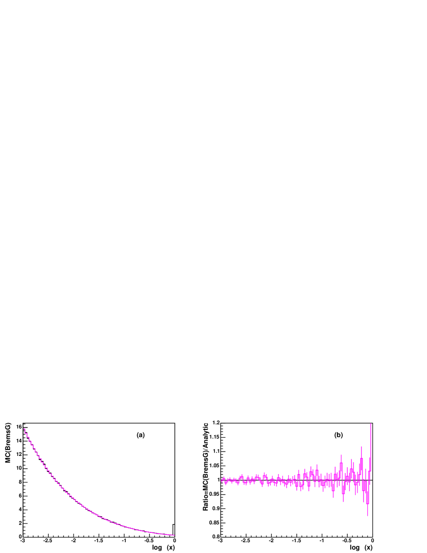
Figure 2: Pure gluon case. $P_{GG}=2C_{A}/z$. The distribution of $x=\prod_{i}z_{i}$ and its ratio to the analytical prediction $B^{\prime}(\gamma,x)$.

As a warming-up exercise, let us now work out in detail a MC algorithm calculating the following integral, cf. eq. (40):

$$I(\gamma)=\int_{\epsilon_{1}}^{1}dx\;d^{B}_{G}(\tau,x|\tau_{0})=\int_{\epsilon_{1}}^{1}dx\frac{1}{x}\;B^{\prime}(\gamma,x),$$ (46)

where $\gamma=(\alpha_{S}(t_{A})/\pi)2C_{A}(\tau-\tau_{0})$ and $\epsilon_{1}\ll 1$.

$$B^{\prime}(\gamma,x)=e^{-\gamma}\Bigg{[}\delta(x-1)+\sum_{n=1}^{\infty}\frac{\gamma^{n}}{n!}\prod_{i=1}^{n}\int_{0}^{1}dz_{i}\;\delta\bigg{(}x-\prod_{j=1}^{n}z_{j}\bigg{)}\Bigg{]}$$ (47)

with the aim of preparing basic tools and setting baseline normalization for the MC algorithm of type II.b (similarly as it was done in ref. [13]). On the one hand, the Bessel-class function $B^{\prime}$ is known analytically in terms of a series (44). On the other hand, the integral $I(\gamma)$ can be rewritten as

$$I(\gamma)=e^{-\gamma}\Bigg{[}1+\sum_{n=1}^{\infty}\frac{\gamma^{n}}{n!}\prod_{i=1}^{n}\int_{\epsilon_{1}}^{1}\frac{dz_{i}}{z_{i}}\;\Theta\bigg{(}\prod_{j=1}^{n}z_{j}-\epsilon_{1}\bigg{)}\Bigg{]},$$ (48)

remembering that $x=\prod_{i}z_{i}$. The above integral is easily implementable in the MC, which treats the $\Theta$ function as a MC weight: $W=\Theta\Big{(}\prod_{j=1}^{n}z_{j}-\epsilon_{1}\Big{)}$. The variable $n$ is generated according to the distribution

$$\bar{I}_{0}=e^{-\gamma},\;\bar{I}_{n>0}=\frac{e^{-\gamma}\gamma^{n}}{n!}\ln^{n}\frac{1}{\epsilon_{1}},~{}~{}~{}~{}\bar{I}=\sum_{n=0}^{\infty}\bar{I}_{n}=e^{-\gamma}e^{-\gamma\ln\epsilon_{1}}.$$ (49)

The variables $z_{i}\in(\epsilon_{1},1)$ are generated according to the distribution $1/z_{i}$. Once we generate suitably long series of MC events $(n;z_{1},z_{2},...,z_{n})$ we calculate the integral using the average weight, with the usual expression $I=\langle W\rangle\bar{I}$. In the same MC run we can also obtain the distribution $B^{\prime}(\gamma,x)/x$, just by examining the histogram of $x=\prod_{i}z_{i}$.

In the LHS plot of fig. 2 we show the (properly normalized) distribution of $x$ from the MC. The acceptance rate $\sim 3\times 10^{-4}$ is rather low – it demonstrates the problem with the $1/z$ component in any MC (also Markovian) in which the starting point of the generation of the emission probability is of the Poisson type. This phenomenon is quite general. Our numerical example shows the evolution from $Q=1$ GeV to $Q=1$ TeV. The average emission multiplicity in the MC run is about 3.4 for $\epsilon_{1}=10^{-3}$. Since the resulting distribution of $x$ is known analytically, we can also examine its ratio to the MC result. In the RHS plot of fig. 2 we show this ratio (for $1.4\times 10^{9}$ events). It is equal to 1, to within the statistical error of order $\sim 1\%$. In the LHS plot we clearly see that the contribution $\sim\delta(x)$ is reproduced by this MC algorithm/program (absent in the analytical program).

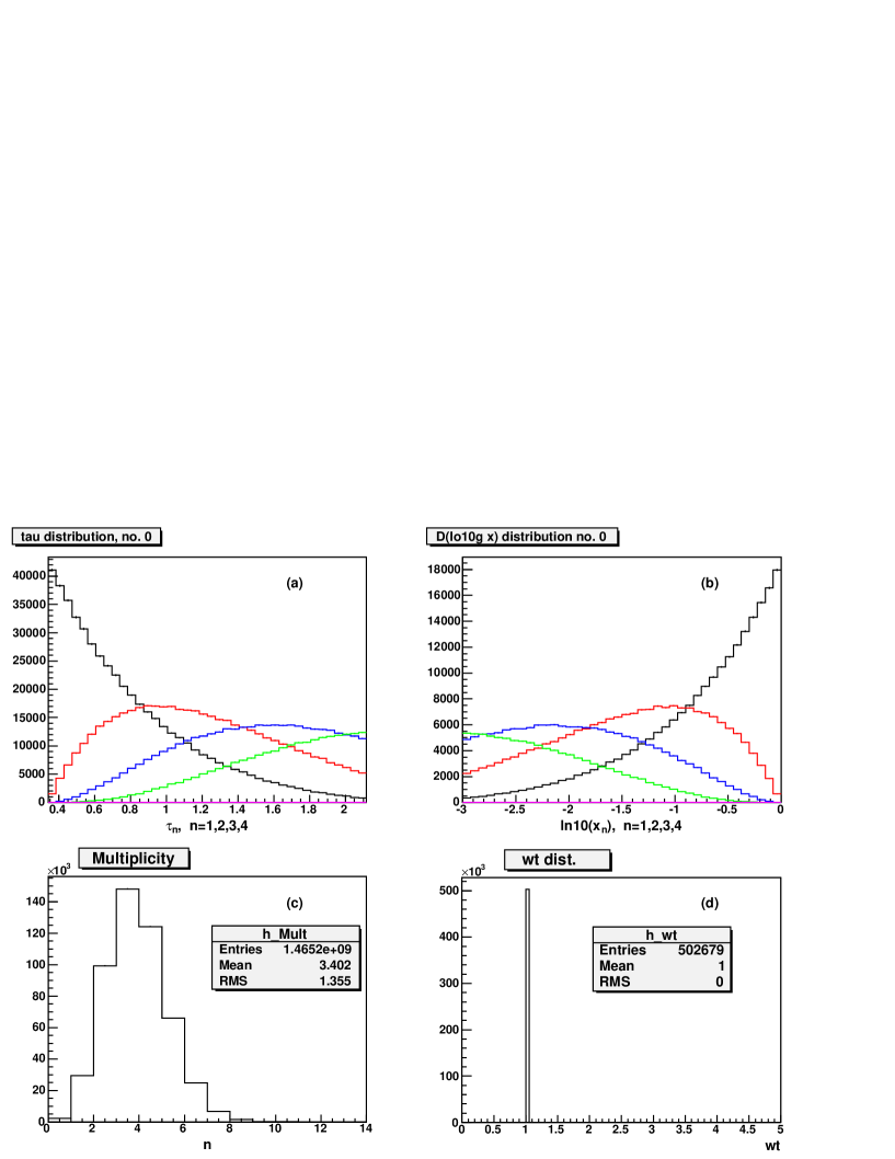
Figure 3: Pure gluon case. Kernel$=2C_{A}/z$. Distribution of the variables $x_{i}=\prod_{n=1}^{i}z_{i}$ and of the ordered $\tau_{i}\in(\tau_{0},\tau)$.

For the purpose of the next exercises we are interested not only in the value of the integral, but also in the exclusive distributions. In fig. 3 we examine the distributions of the first four variables $x_{i}=\prod_{n=1}^{i}$ and $\tau_{i}$ in the emission chain. The ordered $\tau_{i}$ variables are generated within the range $(\tau_{0},\tau)$ corresponding to $Q_{0}=1$ GeV and $Q=1$ TeV. In the following we shall check that the above semi-exclusive distributions are correctly reproduced by more sophisticated MC algorithms. In this figure we also include the distributions of the emission multiplicity and the MC weight. In the weight distribution we exclude zero-weight events.

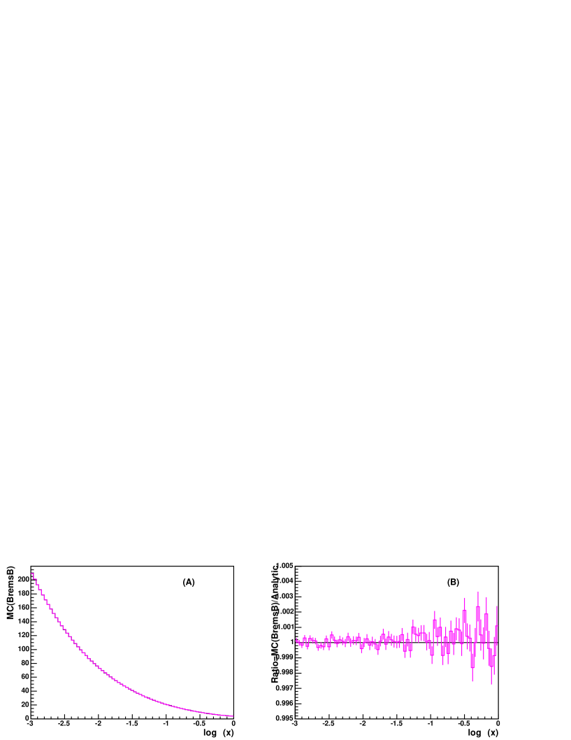
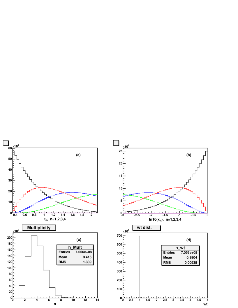
Figure 4: Pure gluon case. Kernel$=2C_{A}/z$. Distribution of the variables $x_{i}=\prod_{n=1}^{i}z_{i}$ and of the ordered $\tau_{i}\in(\tau_{0},\tau)$.

3.3.2 Weight-1 algorithm for $P_{GG}=2C_{A}/z$, Bessel type

The inefficiency of the algorithm described in the previous subsection is mainly due to the fact that the emission probability distribution in the integral under consideration is of the type $P_{n}\sim x^{n}/n!(n-1)!$, Bessel-type for short, while in the MC we actually generate a Poisson distribution $P_{n}\sim x^{n}/n!$ and turn it into a Bessel-type one by the inefficient brute-force rejection method. Now we proceed to the next step – we construct a prototype algorithm in which a Bessel-type emission probability is used from the start and there is no need for the rejection at all. The previous inefficient Poisson-type MC will be useful, however, as a precision cross-check for the new one, especially for testing semi-exclusive distributions.

Let us consider almost the same integral

$$I^{\prime}(\gamma)=\int_{\epsilon_{1}}^{1}dx\frac{1}{x}\;h(x)\;\gamma\;\;_{0}F_{1}(2;-\gamma\ln(x)),$$ (50)

which in the multi-integral form looks as follows:

$$I^{\prime}(\gamma)=\int_{\epsilon_{1}}^{1}dx\frac{1}{x}\;h(x)\;\Bigg{[}\sum_{n=1}^{\infty}\frac{\gamma^{n}}{n!}\prod_{i=1}^{n}\int_{0}^{1}dz_{i}\;\delta\Bigg{(}x-\prod_{j=1}^{n}z_{j}\Bigg{)}\Bigg{]},$$ (51)

where we have removed the unimportant $\delta(1-z)$ component and inserted the test function $h(x)/x$. This integral can be rewritten as

$$I^{\prime}(\gamma)=\int\limits_{\epsilon_{1}}^{1}\frac{dx}{x}h(x)\bigg{[}\sum_{n=1}^{\infty}\frac{\gamma^{n}\ln^{n-1}(1/x)}{n!(n-1)!}\biggl{(}\frac{(n-1)!}{\ln^{n-1}(1/x)}\prod_{i=1}^{n}\int\limits_{0}^{1}d\ln z_{i}\;\delta\Big{(}\ln x-\sum_{j=1}^{n}\ln z_{j}\Big{)}\biggr{)}\bigg{]},$$ (52)

where the internal part of the integrand is conveniently normalized as

$$\frac{(n-1)!}{\ln^{n-1}(1/x)}\;\prod_{i=1}^{n}\int_{0}^{1}d\ln z_{i}\;\delta\Big{(}\ln x-\sum_{j=1}^{n}\ln z_{j}\Big{)}\equiv 1$$ (53)

and we may simulate $z$ variables very easily. Changing variables to $y_{i}=\ln z_{i}$, we see that the distribution in $y_{i}$ is a uniform distribution over the $n-1$ dimensional simplex. There are several convenient methods of generating points uniformly within such a simplex. The simplest method is to throw randomly $n-1$ uniform points $u_{i}\in(\ln x,0),$ $i=1,2,\dots,n-1$ and order them using any standard method: $\ln x=u_{n}<u_{n-1}<\dots<u_{1}<u_{0}=0$. Then we take the differences $y_{i}=u_{i}-u_{i-1}$, $i=1,\dots,n$, which by construction fulfil the constraint $\ln x=\sum_{j=1}^{n}y_{j}$.

The MC algorithm consists of the following steps: first the $x$ is generated according to the distribution

$$\rho(x)=\frac{1}{x}\;h(x)\;\gamma\;\;_{0}F_{1}(2;-\gamma\ln(x)).$$ (54)

Next the number of emissions $n$ is generated according to a (normalized) Bessel-type probability distribution:

$$P_{n}=\Bigl{(}\gamma\;\;_{0}F_{1}(2;-\gamma\ln(x))\Bigr{)}^{-1}\frac{\gamma^{n}\ln^{n-1}(1/x)}{n!(n-1)!},~{}~{}~{}\sum_{n=1}^{\infty}P_{n}=1.$$ (55)

Finally the variables $z_{i}$ are generated as described above. In this algorithm all events are generated with weight 1, provided $x$ is generated exactly according to $\rho(x)$, for instance using the general-purpose tool FOAM. The algorithm is very efficient and fast.

Numerical results from the corresponding MC program are shown in fig. 4. Plot (A) in this figure shows the distribution which is the integrand of eq. (50) from the MC run. The analytical result superimposed on the same plot is indistinguishable from the MC result. In the next plot (B) we show the ratio of the two distributions, MC and analytical. They agree within a very small statistical error of order $\sim 10^{-4}$. In the next two plots, (a) and (b), we see that the new algorithm reproduces perfectly well the semi-exclusive distributions of the same two plots in fig. 3. The multiplicity distribution in the plot (c) is also well reproduced. Plot (d) shows the MC weight distribution.

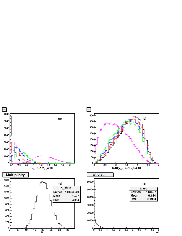
Figure 5: Results from BremsP for the gluon emitter, $k=G$.

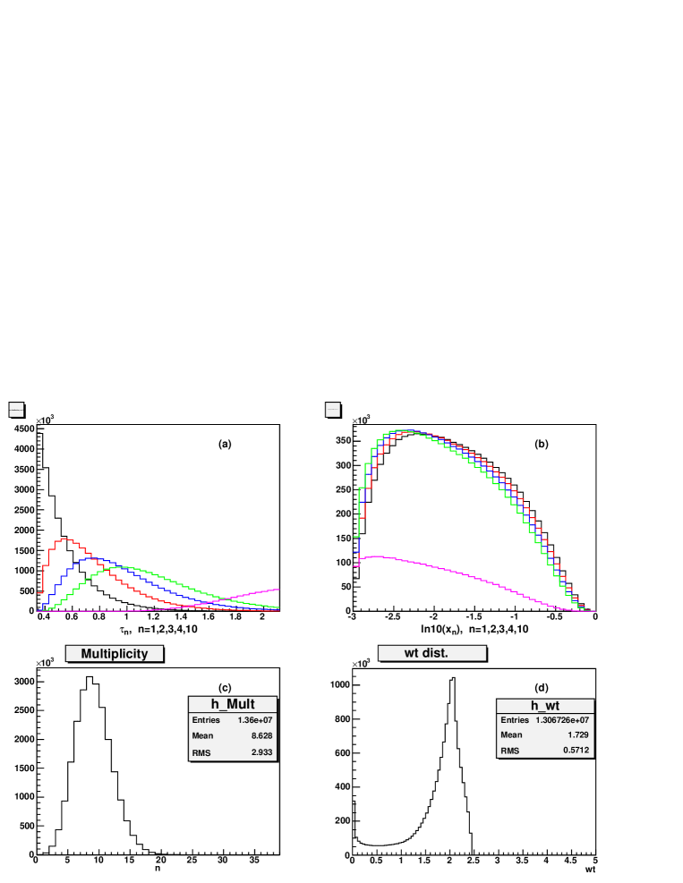
Figure 6: Results from BremsP for quark emitter, $k=Q$.

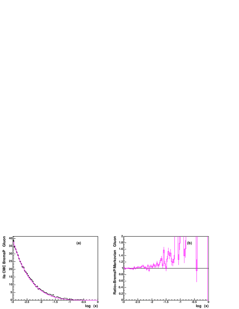
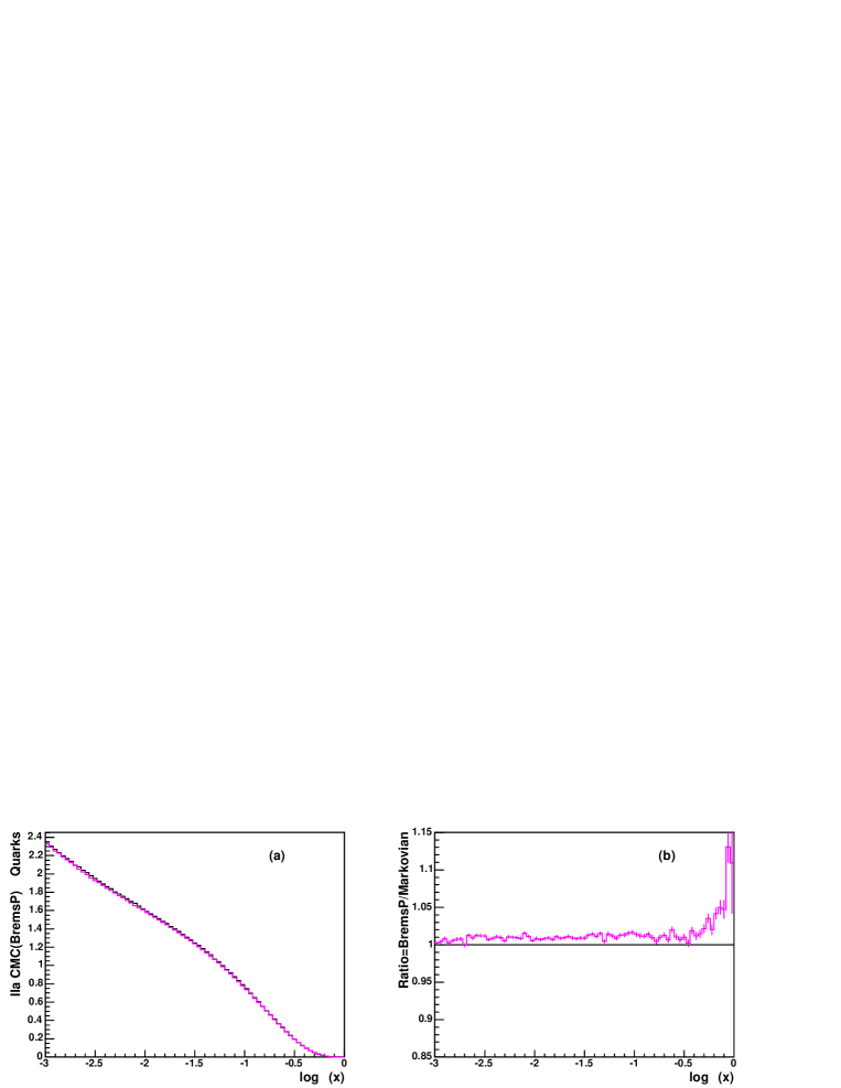
Figure 7: Results from the non-Markovian BremsP (II.a) compared with results of the Markovian EvolMC. Evolution from 1 GeV to 1 TeV due to multiple gluon emission from the gluon emitter line (upper plots) and quark emitter line (lower plots). Starting $D_{k}(\tau_{0},z)$ as in the realistic proton. $N_{f}=3$ in the virtual form factor.

3.3.3 Prototype benchmark type II.a, pure bremsstrahlung

The two toy MCs from previous sections should be regarded as introductory exercises (and numerical benchmarks) for the next step, in which we shall elaborate on the constrained Markovian MC solution with $x$-tagging of the type II.a. We shall restrict ourselves to pure bremsstrahlung from the gluon or quark line, without using the multibranching to isolate $P^{B}_{GG}\sim 1/z$. The corresponding MC prototype we name BremsP. The purpose of that is threefold: (a) to measure the MC efficiency of this class of the MC algorithms, (b) to provide a cross-check for the more sophisticated prototype MC with multibranching for the bremsstrahlung from the gluon line, which will be developed in the next section, (c) to compare it with the other constrained Markovian MC prototypes for the pure bremsstrahlung.

The starting point for the construction of the algorithm is eq. (14). Its simplified version, restricted to the pure bremsstrahlung case, is the following:

$$\begin{split}&\sigma_{k}=\int dx\;H_{k}(x)\;A_{k}x^{-1+\eta}\;e^{-(\tau-\tau_{0})R_{kk}}\sum_{n=0}^{\infty}\;\prod_{i=1}^{n}\;\;\int\limits_{\tau_{i-1}}^{\tau}d\tau_{i}\;\int\limits_{x}^{1}dz_{i}\;\mathcal{P}_{kk}^{\Theta}(z_{i})\;\;\\ &~{}~{}~{}~{}~{}~{}~{}~{}~{}~{}~{}~{}~{}~{}~{}~{}~{}~{}~{}~{}~{}~{}~{}~{}\times W^{\Theta}\;W^{D}_{k}(x,\bar{x}_{0}),\end{split}$$ (56)

where

$$W^{D}_{k}(x,x_{0})=\frac{D_{k}(\tau_{0},x_{0})}{A_{k}x_{0}^{-1+\eta}}\bigg{\{}\frac{x}{\bar{x}_{0}}\bigg{\}}^{-\eta},~{}~{}~{}~{}~{}W^{\Theta}=\Theta\Bigg{(}\prod_{j=1}^{n}z_{j}-x\Bigg{)}.$$ (57)

Neglecting $W^{\Theta}W^{D}$ we can perform a $z$-integration and $n$-summations:

$$\sigma_{k}=\int_{0}^{1}dx\;H_{k}(x)\;A_{k}x^{-1+\eta}\;e^{(\tau-\tau_{0})(-R_{kk}+\Omega_{kk}(x))},~{}~{}~{}~{}\Omega_{kk}(x)=\int\limits_{x}^{1}dz\;\mathcal{P}_{kk}^{\Theta}(z).$$ (58)

The emission multiplicity distribution is Poissonian:

$$P_{n}(x)=\frac{1}{n!}e^{-\lambda(x)}\lambda(x)^{n},~{}~{}~{}~{}~{}\lambda(x)=(\tau-\tau_{0})\Omega_{kk}(z)$$ (59)

and we may generate it together with the $\tau_{i}$ variables, much as in the Markovian case, except that the average multiplicity (forward leap in Markovian random walk) now depends on $x$ (in the unconstrained Markovian it was constant). The variable $x$ is generated as a first variable using FOAM then $n$ and finally $z_{i}\in(x,1)$ exactly according to $\mathcal{P}_{kk}^{\Theta}(z)$.

A few comments on the form factor are in order here. The part $(\tau-\tau_{0})\Omega_{kk}(x)$ is clearly coming from the real emission and, for instance, will be different if we generate according to an approximate $\bar{\mathcal{P}}_{kk}^{\Theta}(z)$; see later in this section. The part $-(\tau-\tau_{0})R_{kk}=-\Phi_{kk}(\tau,\tau_{0})$ is a genuine virtual part of the form factor, independent of any details of the MC generation, cf. eqs. (9)–(10). With the usual expansion

$$P_{ik}(\tau,z)=\delta(1-z)\delta_{ik}A_{kk}+\frac{1}{(1-z)_{+}}\delta_{ik}B_{kk}+\frac{1}{z}C_{ik}+D_{ik}(z),$$ (60)

we obtain

$$R_{kk}=(\tau-\tau_{0})^{-1}\Phi_{kk}(\tau,\tau_{0})=\frac{\alpha_{S}(t_{A})}{\pi}\bigg{[}B_{kk}\ln\frac{1}{\epsilon}-A_{kk}\bigg{]},$$ (61)

and the real emission form factor is

$$\Omega_{kk}(x)=\frac{\alpha_{S}(t_{A})}{\pi}\bigg{[}B_{kk}\ln\frac{1-x}{\epsilon}+C_{kk}\ln\frac{1}{x}+\int_{x}^{1}dz\;D_{kk}(z)\bigg{]},$$ (62)

where

$$\int_{x}^{1}dz\;D_{GG}(z)=2C_{A}\bigg{(}-\frac{11}{6}+x\Big{(}2-\frac{1}{2}x+\frac{1}{3}x^{2}\Big{)}\bigg{)}$$ (63)

and

$$\int_{x}^{1}dz\;D_{qq}(z)=C_{F}\bigg{(}-\frac{3}{2}+x+\frac{1}{2}x^{2}\bigg{)}.$$ (64)

In fig. 5, we show type II.a MC results for the same semi-exclusive distributions as previously, using realistic gluon distribution $D_{G}(\tau_{0},x)=Cx^{-0.8}(1-x)^{5}$, for the gluon-strahlung out of the gluon emitter line. As we see, the efficiency of the MC is extremely low – the acceptance rate is merely $1.5\times 10^{-5}$ (note that the weight-0 events are not included in fig. 5d). Nevertheless, these results will still be useful to cross-check the more efficient algorithm type II.b in the next section. We have investigated what the sources of the inefficiency are. As in the previous toy model, the main reason for low efficiency is that there are many zero-weight events due to $W^{\Theta}$. The factor $(1-x)^{5}$ in the gluon distribution causes a loss of efficiency of a factor 3. The factor $x^{-0.8}$ accounts for a mere factor 2 in the efficiency loss. It is therefore not urgent to eliminate this efficiency by means of incorporating $z^{-\eta}$ factor into $D_{GG}(z)$. This possibility we have considered in the general discussion on method II. On the other hand, a factor 3 loss in the MC efficiency in method II, which is due to the presence of $(1-z)^{5}$ in the gluon SF, looks at first sight irreducible. Nonetheless, one may consider modelling this factor using the internal rejection loop, because the $(1-z)^{5}$ factor, upon expanding, is a sum of monomials $z^{p}$ and the overall normalization can be calculated (with non-MC methods) as a sum over these terms. It is not excluded that with some extra effort, the overall efficiency of the method II.a could be improved to the level of $10^{-4}$.

Let us now repeat the same exercise for the bremsstrahlung emitted from the quark line. In fig. 6 we show the corresponding results ($k=q$) and the starting quark distribution being $D_{q}(\tau_{0},x)=D_{sea}(z)+D_{U}(z)+D_{D}(z)$, that is sea plus both valence quarks, taking a typical parametrization of the proton parton distribution function at $Q_{0}=1$ GeV. Strikingly, the overall efficiency is very good; the rejection rate $\simeq\langle w\rangle/\langle w_{\max}\rangle$ is only about $30\%$! Obviously, without $1/z$ component in the kernel, the basic algorithm type II is quite efficient. It should be remembered that in the actual run $P_{qq}(z)$ is generated exactly (i.e. with the help of the internal rejection loop). The fact that the weight distribution extends above 1, up to 2.5, is related to the valence component. However, the entire weight distribution looks very well for the optional rejection method.

The overall normalization of this MC is cross-checked with the help of the Markovian MC EvolMC of ref. [8]. In the top part of fig. 7 we show result of the evolution from 1 GeV to 1 TeV in which we restrict ourselves to gluon emission out of the gluon line, taking the starting gluon distribution as in the proton. The non-Markovian type II.a MC BremsP reproduces the results of the Markovian MC EvolMC within a statistical error of a few per cent. The apparent discrepancy at high $x$ values is most likely due to some technical bias related to extremely high MC event rejection rate.

In the low part of fig. 7 we present the analogous comparison of BremsP and EvolMC for multiple gluon emission from the quark line. Again, the agreement is quite reasonable, this time within a smaller statistical error of $\sim 1\%$.

As an additional cross-check we also implemented another variant of the II.a type constrained MC algorithm BremsP, with the approximate kernels $\hat{\mathcal{P}}$ and correcting weight applied at the very end of the MC generation. In this case we define

$$\begin{split}&\sigma_{k}=\int dx\;H_{k}(x)\;A_{k}x^{-1+\eta}\;e^{-(\tau-\tau_{0})R_{kk}}\sum_{n=0}^{\infty}\;\prod_{i=1}^{n}\;\;\int\limits_{\tau_{i-1}}^{\tau}d\tau_{i}\;\int\limits_{x}^{1}dz_{i}\;\hat{\mathcal{P}}_{kk}^{\Theta}(z_{i})\;\;\\ &~{}~{}~{}~{}~{}~{}~{}~{}~{}~{}~{}~{}~{}~{}~{}~{}~{}~{}~{}~{}~{}~{}~{}~{}\times W^{\Theta}\;W^{D}_{k}(x,\bar{x}_{0})\;W^{\mathcal{P}}_{k},\end{split}$$ (65)

where the additional weight is

$$W^{\mathcal{P}}_{k}=\prod_{i=0}^{n}\frac{P^{\Theta}(z_{i})}{\hat{P}^{\Theta}(z_{i})}.$$ (66)

Neglecting weights we have

$$\sigma_{k}=\int_{0}^{1}dx\;H_{k}(x)\;A_{k}x^{-1+\eta}\;e^{(\tau-\tau_{0})(-R_{kk}+\hat{\Omega}_{kk}(x))},~{}~{}~{}~{}\hat{\Omega}_{kk}(x)=\int\limits_{x}^{1}dz\;\hat{\mathcal{P}}_{kk}^{\Theta}(z),$$ (67)

where the simplified kernel is defined as

$$\hat{P}_{kk}(t,z)=\delta(1-z)A_{kk}+\frac{1}{(1-z)_{+}}B_{kk}+\frac{1}{z}C_{kk},$$ (68)

leading to the following real emission form factor

$$\hat{\Omega}_{kk}(x)=\frac{\alpha_{S}(t_{A})}{\pi}\bigg{[}B_{kk}\ln\frac{1-x}{\epsilon}+C_{kk}\ln\frac{1}{x}\bigg{]}.$$ (69)

We have checked that the above MC algorithm gives the same quark and gluon distributions, as expected. It is also quite interesting to check how strongly the efficiency of the MC deteriorates when the additional weight $W^{\mathcal{P}}$ is introduced. In the quark case, the acceptance rate drops from 0.7 to 0.25, which is not much, while for gluons it drops by a factor $\sim 10$, well below $10^{-5}$.

In the next step we will clone the MC subgenerator of type II, which generates bremsstrahlung from the quark line according to simplified $\bar{P}^{\Theta}_{qq}=2C_{F}/(1-z)$ and from the gluon line according to “truncated” simplified $\bar{P}^{\Theta A}_{GG}=2C_{A}/(1-z)$. After that, having tested the components at hand, we shall introduce the integration over $Z$ using FOAM and for the bremsstrahlung from the gluon line we shall combine the Bessel’s MC with $P^{\Theta B}_{GG}=2C_{A}/z$ with the above MC for $P^{\Theta A}_{GG}=2C_{A}/(1-z)$ and compare resulting distributions with the Markovian benchmark of fig. 7. This will close the most important first step in making a prototype MC according to method II.b.

3.3.4 Constrained MC type II.b for pure bremsstrahlung

In the following we implement the algorithm II.b in the case of pure bremsstrahlung from the gluon or quark line. In this particular case, the master formula of eq. (39) for the early stage MC (obtained from eq. (36) by neglecting the MC weight) has only one variable $Z^{(1)}$ and $z^{\rm eff}_{\min}=x/Z^{(1)}$. It takes the following simplified form:

$$\begin{split}\bar{\sigma}_{k}=\int_{0}^{1}dx\;&H_{k}(x)\;A_{k}x^{-1+\eta}\;\int\limits_{x}^{1}dZ^{(1)}\;e^{-(\tau-\tau_{0})R^{\prime}_{k}}\;{d^{A}_{k}}^{*}(\tau,z^{\rm eff}_{\min}|\tau_{0})\;\frac{1}{Z^{(1)}}d^{B}_{k}(\tau,Z^{(1)}|\tau_{0}),\\ {d^{A}_{k}}^{*}(\tau,z^{\rm eff}_{\min}|\tau_{0})&=e^{-(\tau-\tau_{0})R^{A}_{kk}}\sum_{n^{\prime}=0}^{\infty}\;\prod_{m=1}^{n^{\prime}}\;\int\limits_{\tau^{\prime}_{m-1}}^{\tau}d\tau^{\prime}_{m}\;\prod_{m=1}^{n^{\prime}}\;\int\limits^{1}_{z^{\rm eff}_{\min}}dz^{\prime}_{m}\;\bar{\mathcal{P}}_{kk}^{\Theta A}(z^{\prime}_{m})\;\\ &=\exp\Biggl{(}-(\tau-\tau_{0})R^{A}_{kk}+(\tau-\tau_{0})\int\limits^{1}_{z^{\rm eff}_{\min}}dz\bar{\mathcal{P}}_{kk}^{\Theta A}(z)\Biggr{)}\\ d^{B}_{q}(\tau,Z^{(1)}|\tau_{0})&=\delta(1-Z^{(1)})\\ d^{B}_{G}(\tau,Z^{(1)}|\tau_{0})&=e^{-(\tau-\tau_{0})R^{B}_{GG}}\bigg{\{}\delta(Z^{(1)}-1)+\\ &+\sum^{\infty}_{n^{\bullet}=1}\;\;\prod_{m=1}^{n^{\bullet}}\int\limits^{\tau}_{\tau^{\bullet}_{m-1}}d\tau^{\bullet}_{m}\;\prod_{m=1}^{n^{\bullet}}\int\limits^{1}_{0}dz_{m}^{\bullet}\;\bar{\mathcal{P}}_{GG}^{\Theta B}(z_{m}^{\bullet})\;\delta\Big{(}Z^{(1)}-\prod_{m=0}^{n^{\bullet}}z_{m}^{\bullet}\Big{)}\bigg{\}}\\ &=\frac{1}{Z^{(1)}}B^{\prime}\Big{(}(\tau-\tau_{0})R^{B}_{GG},Z^{(1)}\Big{)}\\ &=e^{-(\tau-\tau_{0})R^{B}_{GG}}\bigl{(}\delta(Z^{(1)}-1)+\hat{d}^{B}_{G}(\tau,Z^{(1)}|\tau_{0})\bigr{)},\\ \hat{d}^{B}_{G}(\tau,Z^{(1)}|\tau_{0})&=\frac{1}{Z^{(1)}}(\tau-\tau_{0})R^{B}_{GG}\;{}_{0}F_{1}\bigl{(}2;-(\tau-\tau_{0})R^{B}_{GG}\ln(Z^{(1)})\bigr{)}.\end{split}$$ (70)

The integral proportional to $\delta(1-Z^{(1)})$ has to be treated separately:

$$\begin{split}\bar{\sigma}_{q}&=\int_{0}^{1}dx\;H_{q}(x)\;A_{q}x^{-1+\eta}\;e^{-(\tau-\tau_{0})R^{\prime}_{q}}\;{d^{A}_{q}}^{*}(\tau,x|\tau_{0}),\\ \bar{\sigma}_{G}&=\int_{0}^{1}dx\;H_{G}(x)\;A_{G}x^{-1+\eta}\int\limits^{1}_{x}\frac{dZ^{(1)}}{Z^{(1)}}e^{-(\tau-\tau_{0})R^{\prime}_{G}}\;{d^{A}_{G}}^{*}\Bigl{(}\tau,\frac{x}{Z^{(1)}}\Big{|}\tau_{0}\Bigr{)}\;e^{-(\tau-\tau_{0})R^{B}_{GG}}\hat{d}^{B}_{G}(\tau,Z^{(1)}|\tau_{0})\\ &+\int\limits_{0}^{1}dx\;H_{G}(x)\;A_{G}x^{-1+\eta}\;e^{-(\tau-\tau_{0})R^{\prime}_{G}}\;{d^{A}_{G}}^{*}(\tau,x|\tau_{0})e^{-(\tau-\tau_{0})R^{B}_{GG}}.\end{split}$$ (71)

The distribution of the variables $x$ and $Z=Z^{(1)}$ for the general-purpose simulator FOAM are given by the integrands in the integrals:

$$\begin{split}\bar{\sigma}_{q}&=\int\limits_{0}^{1}dx\int\limits^{1}_{x}dZ\;H_{q}(x)\;A_{q}x^{-1+\eta}\;\exp\Biggl{[}-(\tau-\tau_{0})\biggl{(}R^{\prime}_{q}+R^{A}_{qq}-\int\limits^{1}_{x}dz\bar{\mathcal{P}}_{qq}^{\Theta A}(z)\biggr{)}\Biggr{]},\\ \bar{\sigma}_{G}&=\int\limits_{0}^{1}dx\int\limits^{1}_{x}\frac{dZ}{Z}\;H_{G}(x)\;A_{G}x^{-1+\eta}\;\\ &\hskip 85.35826pt\exp\Biggl{[}-(\tau-\tau_{0})\biggl{(}R^{\prime}_{G}+R^{A}_{GG}+R^{B}_{GG}-\int\limits^{1}_{x/Z}dz\bar{\mathcal{P}}_{GG}^{\Theta A}(z)\biggr{)}\Biggr{]}\hat{d}^{B}_{G}(\tau,Z|\tau_{0})\\ &+\int\limits_{0}^{1}dx\;H_{G}(x)\;A_{G}x^{-1+\eta}\;\exp\Biggl{[}-(\tau-\tau_{0})\biggl{(}R^{\prime}_{G}+R^{B}_{GG}+R^{A}_{GG}-\int\limits^{1}_{x}dz\bar{\mathcal{P}}_{GG}^{\Theta A}(z)\biggr{)}\Biggr{]}.\end{split}$$ (72)

Keeping in mind that $R^{B}_{qq}=0$, we recover in eq. (72) the complete virtual form factor $R_{k}$

$$R^{\prime}_{k}+R^{A}_{kk}+R^{B}_{kk}=R_{k}=(\tau-\tau_{0})^{-1}\Phi_{k}(\tau,\tau_{0})=\frac{\alpha_{S}(t_{A})}{\pi}\bigg{[}B_{kk}\ln\frac{1}{\epsilon}-A_{kk}\bigg{]},$$ (73)

see eq. (61). Finally we arrive at the following expression:

$$\begin{split}\bar{\sigma}_{q}&=\int\limits_{0}^{1}dx\int\limits^{1}_{x}dZ\;H_{q}(x)\;A_{q}x^{-1+\eta}\;e^{-(\tau-\tau_{0})\bigl{(}R_{q}-\bar{\Omega}^{A}_{q}(x)\bigr{)}}\\ &=\bar{\sigma}^{(a)}_{q},\;\;\;\bar{\sigma}^{(b)}_{q}=0,\\ \bar{\sigma}_{G}&=\int\limits_{0}^{1}dx\int\limits^{1}_{x}\frac{dZ}{Z}\;H_{G}(x)\;A_{G}x^{-1+\eta}\;e^{-(\tau-\tau_{0})\bigl{(}R_{G}-\bar{\Omega}^{A}_{G}(x/Z)\bigr{)}}\hat{d}^{B}_{G}(\tau,Z|\tau_{0})\\ &+\int\limits_{0}^{1}dx\;H_{G}(x)\;A_{G}x^{-1+\eta}\;e^{-(\tau-\tau_{0})\bigl{(}R_{G}-\bar{\Omega}^{A}_{G}(x)\bigr{)}}\\ &=\bar{\sigma}^{(a)}_{G}+\bar{\sigma}^{(b)}_{G}.\end{split}$$ (74)

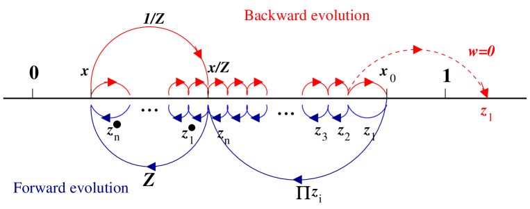
Figure 8: Scheme of the II.b MC algorithm in x space before relabelling, for the case of pure bremsstrahlung. $x_{0}=x/(Z\prod_{i}z^{\prime}_{i})$ results from $Z$ and $\prod z_{i}$. The zero-weight case of $x_{0}>1$ is also indicated.

The MC algorithm of type II.b for generating single (weighted) MC event consists of the following steps:

1. Generate a branch index $X=a,b$ according to a probability proportional to $\bar{\sigma}_{k}^{(X)}$; FOAM does that efficiently.

2. For given $X$ generate variables $x$ and $Z$ or only $x$ according to the integrand of the corresponding integral $\bar{\sigma}_{k}^{(X)}$; also done by FOAM.

3. In the case $X=a$ generate two emission multiplicities $n^{\prime}$ and $n^{\bullet}$, the first one according to the Poisson distribution with $\langle n^{\prime}\rangle=(\tau-\tau_{0})\Omega^{A}_{k}(x/Z)$ and the other one according to the Bessel-type distribution with $\lambda=(\tau-\tau_{0})R^{B}_{GG}\ln(1/Z)$ (as in the toy models).

4. Knowing the multiplicities, generate the variables $(\tau^{\prime}_{i},z^{\prime}_{i}),~{}i=1,\dots,n^{\prime}$ and $(\tau^{\bullet}_{j},z^{\bullet}_{j}),~{}j=1,\dots,n^{\bullet}$, using methods described earlier.

5. Relabel the emission vertices, guided by the order of the $\tau$ variables.

6. Calculate the final MC weight, the same as was neglected at the early stage of generating “phase-space” variables.

The above algorithm is also illustrated schematically in fig. 8, in the $x$-space, before the relabelling. Arrows help to understand the order of the reconstruction of all $x$ variables out of $z$ variables.

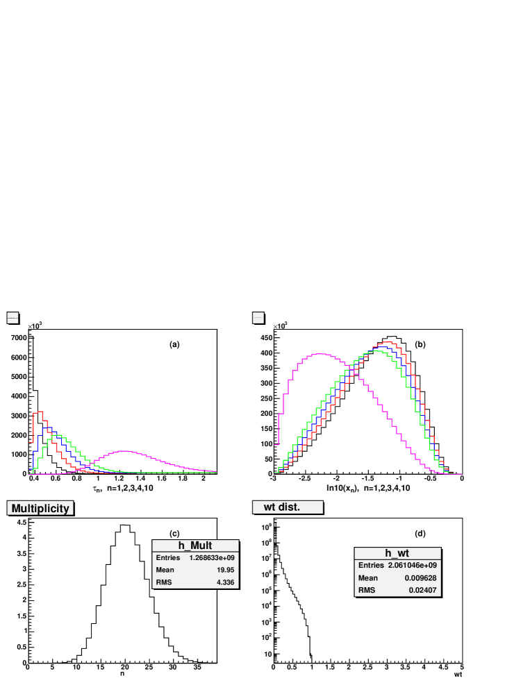
Figure 9: Results form GenIIb MC prototype for gluon emitter, $k=G$.

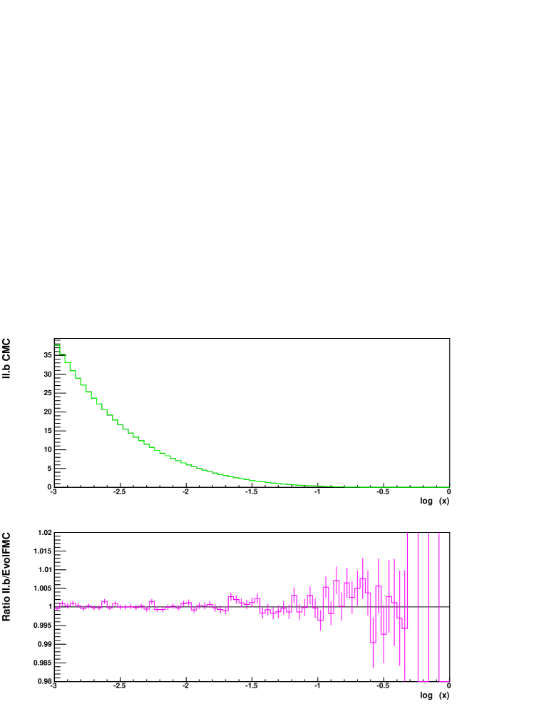
Figure 10: Comparison of II.b MC GenIIb with the Markovian MC EvolMC for pure gluonstrahlung $k=G$, $D_{G}(\tau_{0},z)$ as in proton. $N_{f}=0$.

In fig. 9 we show numerical results for the II.b prototype MC for the same semi-exclusive $x$- and $\tau$-distributions as previously. MC results coincide very well with these from BremsP in figs. 5. This is a highly non-trivial result, having in mind sophistication of the algorithm II.b. Let us stress that the above agreement cannot be obtained without a correct relabelling procedure being performed in the final stage of the algorithm II.b .

The generation time of an event (before any rejections) is similar for both algorithms II.a and II.b. Therefore the acceptance, i.e. the ratio of the average to maximum weight, is a good measure of the overall efficiency of the algorithms. The acceptance for the new algorithm type II.b, as read from the weight distribution in fig. 9 is $9.6\times 10^{-3}$. This is a little bit worse than expected; it is, however, fully satisfactory – it is better by a factor of $500$ than the efficiency $2\times 10^{-5}$ for the solution II.a (without multibranching), see fig. 5. Using algorithm II.a as a guide, one may argue that the $9.6\times 10^{-3}$ efficiency can still be improved by a factor of 2 by including exactly the $x_{0}^{-0.8}$ factor. Another factor of 3 could be obtained by performing a modelling of the $(1-x_{0})^{5}$ distribution in an internal rejection loop of the algorithm. In this way the overall efficiency may go up to the level of 5%.

Plots in fig. 9 show tests of exclusive distributions and efficiency, but not the overall normalization. A strong test of the overall normalization of the algorithm II.b is shown in fig. 10, where high statistics ($\sim 4\times 10^{9}$ events) results of the II.b MC are compared with those of the forward Markovian MC EvolMC of ref. [8]. The agreement is reached within a statistical error of about 0.1% for $x<0.01$ and of 0.3% for $x<0.1$. For higher $x$, in spite of the extreme smallness of $D_{G}(x)$ (over 9 orders of magnitude), the agreement holds perfectly well within the statistical errors.

At this point we may state that our method II.b of solving the constrained MC really works in practice and is reasonably efficient.

We want to stress that it would not be possible to reach this conclusion without constructing and testing the explicit prototype of the algorithm type II.a, and other auxiliary MC exercises, as we did in this work.

In the above numerical exercises we have restricted ourselves to the LL case, with $N_{f}=3$ massless quarks. The QCD evolution kernels are unique and well known, and we therefore skip their explicit definition. The running constant $\alpha_{S}(t)=2\pi/(\beta_{0}(t-\ln\Lambda_{0}))$ was used with $\Lambda_{0}=0.245748338$. The following starting values of the parton distributions in proton at $Q_{0}=1$ GeV were used in all our numerical exercises:

$$\begin{split}xD_{G}(Q_{0},x)&=1.9083594473\cdot x^{-0.2}(1-x)^{5.0},\\ xD_{q}(Q_{0},x)&=0.5\cdot xD_{\rm sea}(x)+xD_{2u}(x),\\ xD_{\bar{q}}(Q_{0},x)&=0.5\cdot xD_{\rm sea}(x)+xD_{d}(x),\\ xD_{\rm sea}(Q_{0},x)&=0.6733449216\cdot x^{-0.2}(1-x)^{7.0},\\ xD_{2u}(Q_{0},x)&=2.1875000000\cdot x^{0.5}(1-x)^{3.0},\\ xD_{d}(Q_{0},x)&=1.2304687500\cdot x^{0.5}(1-x)^{4.0}.\end{split}$$ (75)

4 Summary

In this paper we presented a MC algorithm, which belongs to a new class of MC algorithms capable of generating a constrained Markovian evolution of parton distributions according to DGLAP evolution equations. Practical numerical implementation is for the moment restricted to the pure bremsstrahlung case. Since the algebraic framework is defined for the full DGLAP, it is therefore a matter of more programming to extend it to the general case. In the presented numerical tests (pure bremsstrahlung) the algorithm has been checked against the dedicated forward evolution (Markovian) MC program that we have written. We found an agreement at the level of 0.1%. The measured efficiency of the constrained MC is found to be quite satisfactory. This work opens the way to a new class of MC algorithms with possible applications in the initial-state QCD parton shower MC. Furthermore, the Bessel-type distribution of the number of emissions, which forms the core of our algorithms, is similar to this obtained from the CCFM approach [19], as shown in [18]. This suggests another possible area of applications of our algorithms.

Acknowledgements
We would like to thank W. Płaczek and T. Sjöstrand for useful discussions. We thank, for their warm hospitality, the CERN Particle Theory Group, where part of this work was done.

APPENDIX

The technique of the kernel split (multibranching)

In section 3.2.2 we have shown how to reorganize integration variables in the evolution iterative solution, such that in the Monte Carlo integration/simulation algorithm it is possible to generate first the chain of flavour indexes (gluon or quark type) and the corresponding evolution time variables $\tau_{i}$ (i.e. those of the emissions which change flavour), and later the other variables corresponding to gluon emissions (no flavour change).

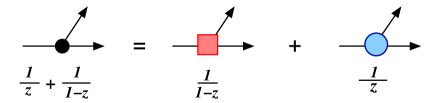
Figure 11: Graphical representation of the split of the (approximate) gluon emission kernel into two parts.

In the following we shall describe the application of the MC technique of multibranching to our problem. In the multibranching one splits the integrand into many positive components, chooses randomly one at a time and generates points according to this particular component. In the context of the iterative solution of the evolution equation, it is worthwhile to apply this technique to the kernel for the transition of the gluon into gluon:

$$P_{GG}(z)=2C_{A}\left[\frac{z}{1-z}+\frac{1-z}{z}+z(1-z)\right],$$ (76)

which has two very different singularities $1/z$ and $1/(1-z)$. Therefore it is profitable in the Monte Carlo to split $P_{GG}(z)=P^{A}_{GG}(z)+P^{B}_{GG}(z)$ such that $P^{A}_{GG}(z)\sim 1/(1-z)$ and $P^{B}_{GG}\sim 1/z$ (see fig. 11), and to generate them separately, applying additional MC methods suited to the individual character of each type of singularity.

Since we already know from section 3.2.2 how to isolate the pure bremsstrahlung subintegrals $d^{\prime}_{k}$; see eq. (15), let us concentrate on one of them:

$$\begin{split}d^{\prime}_{k}(\tau,x|\tau_{0})=&e^{-(\tau-\tau_{0})R_{kk}}\delta(x-1)+\sum_{n=1}^{\infty}\Biggl{(}\prod_{j=1}^{n}\int\limits_{\tau_{0}}^{\tau}d\tau_{j}\;\Theta(\tau_{j}-\tau_{j-1})\int\limits_{0}^{1}dz_{j}\Biggr{)}\\ &\times e^{-(\tau-\tau_{n})R_{kk}}\Biggl{(}\prod_{i=1}^{n}{\cal P}_{kk}^{\Theta}(z_{i})\;e^{-(\tau_{i}-\tau_{i-1})R_{kk}}\Biggr{)}\delta\bigg{(}x-\prod_{i=1}^{n}z_{i}\bigg{)},\end{split}$$ (77)

where in reality we are interested in the gluon case ${\cal P}_{kk}(z)={\cal P}_{GG}(z)$.

Taking advantage of the independence of the kernels on $\tau$ we can rewrite the above equation as follows:

$$\begin{split}d^{\prime}_{k}(\tau,x|\tau_{0})&=e^{-(\tau-\tau_{0})R_{kk}}\sum_{n=0}^{\infty}\frac{(\tau-\tau_{0})^{n}}{n!}\prod_{i=1}^{n}\int\limits_{0}^{1}dz_{i}\;\\ &\times\prod_{i=1}^{n}[{\cal P}_{kk}^{\Theta A}(z_{i})+{\cal P}_{kk}^{\Theta B}(z_{i})]\;\delta\bigg{(}x-\prod_{i=1}^{n}z_{i}\bigg{)},\end{split}$$ (78)

where more compact notation is achieved by defining $\prod\limits_{i=1}^{0}\equiv 1$. Note that at this stage we made certain important short-cuts, because we have integrated over $\tau$. This simplifies the argument but makes it questionable in view of certain important claims concerning the final distribution in the space of $(n;\tau_{1},z_{1},\tau_{2},z_{2},...,\tau_{n},z_{n})$, which we are going to make at the end of this appendix. We shall therefore refine our proof later on, showing how to proceed for the distributions with unintegrated $\tau$’s.

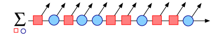
Figure 12: Reorganization of the multiple gluon emission leading to multibranching.

Let us now reorganize the overall sum as follows (see also schematic illustration in fig. 12),

$$\begin{split}d^{\prime}_{k}(\tau,x|\tau_{0})&=e^{-(\tau-\tau_{0})R_{kk}}\sum_{n_{1}=0}^{\infty}\sum_{n_{2}=0}^{\infty}\frac{(\tau-\tau_{0})^{n_{1}+n_{2}}}{n_{1}!n_{2}!}\prod_{i=1}^{n_{1}}\int\limits_{0}^{1}dz_{i}\;\prod_{j=1}^{n_{2}}\int\limits_{0}^{1}dz_{j}\;\\ &\times\prod_{i=1}^{n_{1}}{\cal P}_{kk}^{\Theta A}(z_{i})\;\prod_{j=1}^{n_{2}}{\cal P}_{kk}^{\Theta B}(z_{j})\;\;\delta\bigg{(}x-\prod_{i=1}^{n_{1}}z_{i}\prod_{j=1}^{n_{2}}z_{j}\bigg{)},\end{split}$$ (79)

where the two sums take care of the two kernel components. We can now factorize the whole integral as a convolution of the two integrals, each of them corresponding to one component of the kernel:

$$\begin{split}&d^{\prime}_{k}(\tau,x|\tau_{0})=\int_{0}^{1}dz^{A}\int_{0}^{1}dz^{B}\;\delta(x-z^{A}z^{B})\;d^{\prime A}_{k}(\tau,z^{A}|\tau_{0})\;d^{\prime B}_{k}(\tau,z^{B}|\tau_{0}),\\ &d^{\prime X}_{k}(\tau,x|\tau_{0})=e^{-(\tau-\tau_{0})R^{X}_{kk}}\sum_{n=0}^{\infty}\frac{(\tau-\tau_{0})^{n}}{n!}\prod_{i=1}^{n}{\cal P}_{kk}^{\Theta X}(z_{i})\;\delta\bigg{(}x-\prod_{j=1}^{n}z_{j}\bigg{)},\;\;X=A,B.\end{split}$$ (80)

The functions $R^{X}$ are constrained only by

$$\sum_{X}R^{X}_{kk}=R_{kk}.$$ (81)

For example in some cases they may be defined as

$$R^{X}_{kk}=\int_{0}^{1-\varepsilon}dzz{\cal P}_{kk}^{\Theta X}(z).$$ (82)

We may restore the ordered evolution time integrals

$$d^{\prime X}_{k}(\tau,x|\tau_{0})=e^{-(\tau-\tau_{0})R^{X}_{kk}}\sum_{n=0}^{\infty}\prod_{j=1}^{n}\int\limits_{\tau_{0}}^{\tau}d\tau_{j}\;\Theta(\tau_{j}-\tau_{j-1})\prod_{i=1}^{n}{\cal P}_{kk}^{\Theta X}(z_{i})\;\delta\bigg{(}x-\prod_{j=1}^{n}z_{j}\bigg{)}.$$ (83)

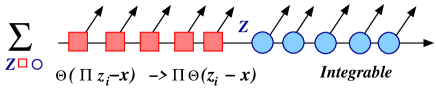
Figure 13: Further reorganization of the multiple gluon emission in the multibranching.

However, it should be remembered that the variables $\tau_{i}$ and $z_{i}$ are not exactly the same as in the original integral (in spite of the same notation) but they are related by means of a “relabelling” procedure described later in this appendix. The above algebra is represented schematically in fig. 13.

It is now possible to implement the integral of eq. (80) as a pair of two independent “parallel Markovian processes”, both starting at $\tau_{0}$ and stopping at $\tau$. The first one would have decay constant $R^{A}_{kk}$ and variable $z_{i}$ generated according to ${\cal P}_{kk}^{\Theta A}(z_{i})$, yielding emission multiplicity $n_{1}$ at the stopping point, while the second one would have its decay constant $R^{B}_{kk}$, variables $z_{j}$ generated according to ${\cal P}_{kk}^{\Theta B}(z_{j})$, and the emission multiplicity $n_{2}$.

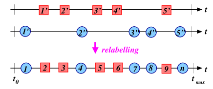
Figure 14: Illustration of “relabelling”. The actual generation is done in two steps: First, for each of the two branches (squares and circles) the ordered $\tau$’s are generated separately and independently in the entire $\tau$-range. Next, $(\tau_{i},z_{i})$ are relabelled according to a common ordering in $\tau$. Only after such a relabelling is $x$ constructed: $x=\prod^{n}_{j=1}z_{j}$.

It is important to understand that at the very end the two sets of $z_{i},\tau_{i}$, $i=1,...,n_{1}$ and $z_{j},\tau_{j}$, $j=1,...,n_{2}$ can be merged, forgetting from which parallel generation branch they originate. Merging is done simply by creating a common list of ordered variables $\tau_{i}$ and renaming/reordering $z_{i}$ variables in exactly the same way. Such relabelling procedure will undo the procedure of combining together the $\left({n_{1}+n_{2}\atop n_{1}}\right)$ terms done in eq. (79). The relabelling procedure is illustrated schematically in fig. 14. The resulting $z_{l}$, $l=1,...,n_{1}+n_{2}$ will be then distributed according to the product

$$\prod_{l=1}^{n_{1}+n_{2}}[{\cal P}_{kk}^{\Theta A}(z_{l})+{\cal P}_{kk}^{\Theta B}(z_{l})]$$ (84)

Moreover, also the total multiplicity $n=n_{1}+n_{2}$ and the evolution times $\tau_{l}$, $l=1,...,n$ will be distributed as if they were coming from the corresponding single Markovian MC.

Actually, the reader may be concerned that the above claim is not really founded on a solid derivation because we have excluded the $\tau$ space in the binomial decomposition after integrating over $\tau$’s at an early stage of derivation, while we are now making statements on the distribution in the full space $\tau_{1},z_{1},\tau_{2},z_{2},...,\tau_{n},z_{n}$. We need clearly to refine our derivation keeping the $\tau$-space alive. The full derivation involves non-trivial combinatorics, and here we shall only give a sketch on the necessary reasoning. Consider the expression with three kernels

$$\begin{split}&\int d\tau_{1}d\tau_{2}d\tau_{3}\Theta_{321}\int dz_{1}dz_{2}dz_{3}(A(3)+B(3))(A(2)+B(2))(A(1)+B(1)),\end{split}$$ (85)

where we abbreviate: $\Theta_{321}=\Theta(\tau_{3}-\tau_{2})\Theta(\tau_{2}-\tau_{1})$ and $A(i)=\mathcal{P}_{kk}^{A}(z_{i})$, $B(j)=\mathcal{P}_{kk}^{B}(z_{j})$. It is decomposed as follows

$$\begin{split}\int d\tau_{1}d\tau_{2}d\tau_{3}\Theta_{321}\int dz_{1}dz_{2}dz_{3}&[A(3)A(2)A(1)\\ &+B(3)A(2)A(1)+A(3)B(2)A(1)+A(3)A(2)B(1)\\ &+B(3)B(2)A(1)+B(3)A(2)B(1)+A(3)B(2)B(1)\\ &+B(3)B(2)B(1)]\end{split}$$ (86)

Each of the four groups in four lines is now transformed separately into a single factor with different ordering pattern of the $\tau$ variables. For instance the second line we transform explicitly as follows:

$$\begin{split}\int&d\tau_{1}d\tau_{2}d\tau_{3}\Theta_{321}\int dz_{1}dz_{2}dz_{3}[B(3)A(2)A(1)+A(3)B(2)A(1)+A(3)A(2)B(1)]\\ &=\int d\tau_{1}d\tau_{2}d\tau_{1^{\prime}}dz_{1}dz_{2}dz_{1^{\prime}}\Theta_{1^{\prime}21}B(1^{\prime})A(2)A(1)\\ &+\int d\tau_{1}d\tau_{1^{\prime}}d\tau_{3}dz_{1}dz_{1^{\prime}}dz_{3}\Theta_{31^{\prime}1}A(3)B(1^{\prime})A(1)\\ &+\int d\tau_{1^{\prime}}d\tau_{2}d\tau_{3}dz_{1^{\prime}}dz_{2}dz_{3}\Theta_{321^{\prime}}A(3)A(2)B(1^{\prime})]\end{split}$$ (87)

where we essentially renamed both $z$’s and $\tau$’s sitting in the $B$-factor. The same can be done for variables in the $A$-factors:

$$\begin{split}&\int d\tau^{\bullet}_{1}d\tau^{\bullet}_{2}d\tau^{\prime}_{1}dz^{\bullet}_{1}dz^{\bullet}_{2}dz^{\prime}_{1}\Theta_{1^{\prime}2^{\bullet}1^{\bullet}}B(1^{\prime})A(2^{\bullet})A(1^{\bullet})\\ +&\int d\tau^{\bullet}_{1}d\tau^{\prime}_{1}d\tau^{\bullet}_{2}dz^{\bullet}_{1}dz^{\prime}_{1}dz^{\bullet}_{2}\Theta_{2^{\bullet}1^{\prime}1^{\bullet}}A(2^{\bullet})B(1^{\prime})A(1^{\bullet})\\ +&\int d\tau^{\prime}_{1}d\tau^{\bullet}_{1}d\tau^{\bullet}_{2}dz^{\prime}_{1}dz^{\bullet}_{1}dz^{\bullet}_{2}\Theta_{2^{\bullet}1^{\bullet}1^{\prime}}A(2^{\bullet})A(1^{\bullet})B(1^{\prime})].\end{split}$$ (88)

Let us summarize explicitly the relabelling of the variables that has been done above:

$$\begin{split}\hbox{\rm for}~{}~{}~{}\tau^{\prime}_{1}>\tau^{\bullet}_{2}>\tau^{\bullet}_{1}:~{}~{}~{}~{}&\tau_{1}=\tau^{\prime}_{1},\;\tau_{2}=\tau^{\bullet}_{2},\;\tau_{1}=\tau^{\bullet}_{1},~{}~{}z_{1}=z^{\prime}_{1},\;z_{2}=z^{\bullet}_{2},\;z_{1}=z^{\bullet}_{1},\\ \hbox{\rm for}~{}~{}~{}\tau^{\bullet}_{2}>\tau^{\prime}_{1}>\tau^{\bullet}_{1}:~{}~{}~{}~{}&\tau_{1}=\tau^{\bullet}_{2},\;\tau_{2}=\tau^{\prime}_{1},\;\tau_{1}=\tau^{\bullet}_{1},~{}~{}z_{1}=z^{\bullet}_{2},\;z_{2}=z^{\prime}_{1},\;z_{1}=z^{\bullet}_{1},\\ \hbox{\rm for}~{}~{}~{}\tau^{\bullet}_{2}>\tau^{\bullet}_{1}>\tau^{\prime}_{1}:~{}~{}~{}~{}&\tau_{1}=\tau^{\bullet}_{2},\;\tau_{2}=\tau^{\bullet}_{1},\;\tau_{1}=\tau^{\prime}_{1},~{}~{}z_{1}=z^{\bullet}_{2},\;z_{2}=z^{\bullet}_{1},\;z_{1}=z^{\prime}_{1},\end{split}$$ (89)

Now, we may pull out the kernels and combine the $\Theta$-functions

$$\begin{split}\int&d\tau^{\bullet}_{1}d\tau^{\bullet}_{2}d\tau^{\prime}_{1}dz^{\bullet}_{1}dz^{\bullet}_{2}dz^{\prime}_{1}B(1^{\prime})A(2^{\bullet})A(1^{\bullet})[\Theta_{1^{\prime}2^{\bullet}1^{\bullet}}+\Theta_{2^{\bullet}1^{\prime}1^{\bullet}}+\Theta_{2^{\bullet}1^{\bullet}1^{\prime}}]\\ &=\int d\tau^{\bullet}_{1}d\tau^{\bullet}_{2}d\tau^{\prime}_{1}\;dz^{\bullet}_{1}dz^{\bullet}_{2}dz^{\prime}_{1}\;\;\Theta_{2^{\bullet}1^{\bullet}}A(2^{\bullet})A(1^{\bullet})\;\;\Theta^{\prime}_{1}B(1^{\prime}),\end{split}$$ (90)

where $\Theta_{1^{\prime}}=1$ and $\Theta_{2^{\bullet}1^{\bullet}}=\Theta(\tau^{\bullet}_{2}-\tau^{\bullet}_{1})$. The above tedious relabelling of $z$’s and $\tau$’s and recombining of $\Theta$’s into product of two independent ones can be done for any number of kernels. The net result is an interesting identity:

$$\begin{split}\prod_{i=1}^{n}\int_{\tau_{i-1}}^{1}d\tau_{i}&\int_{0}^{1}dz_{i}\;(A(z_{i})+B(z_{i}))w({\bf\tau},{\bf z})\\ =\sum_{n_{1}=0}^{n}&\left(\prod_{i=1}^{n_{1}}\int_{\tau^{\bullet}_{i-1}}^{1}d\tau^{\bullet}_{i}\int_{0}^{1}dz^{\bullet}_{i}\;A(z^{\bullet}_{i})\right)\;\;\left(\prod_{i=1}^{n-n_{1}}\int_{\tau^{\prime}_{i-1}}^{1}d\tau^{\prime}_{i}\;\int_{0}^{1}dz^{\prime}_{i}\;A(z^{\prime}_{i})\right)\\ &w\bigl{(}{\bf\mbox{\boldmath$\tau$}(\mbox{\boldmath$\tau$}^{\bullet},\mbox{\boldmath$\tau$}^{\prime})},{\bf z(\mbox{\boldmath$\tau$}^{\bullet};\mbox{\boldmath$\tau$}^{\prime},z^{\bullet},z^{\prime})}\bigr{)},\end{split}$$ (91)

where $w(\mbox{\boldmath$\tau$},{\bf z})$ is an arbitrary “test function” ensuring that eq.  (91) is indeed a differential identity, and not an obvious multiplication rule of exponential functions. The mapping (relabelling) $\tau_{i}=\tau_{i}({\bf\mbox{\boldmath$\tau$}^{\bullet},\mbox{\boldmath$\tau$}^{\prime}})$ and $z_{i}=z_{i}({\bf\mbox{\boldmath$\tau$}^{\bullet};\mbox{\boldmath$\tau$}^{\prime},z^{\bullet},z^{\prime}})$ is nothing more than a permutation of the integration variables, which is “guided” by the ordering of the $\tau$ variables, much as in the explicit example above. Note that the above identity is still valid if the integrand involves any additional factor, symmetric with respect to the permutation of the integrand variables $\tau_{i}$ and $z_{i}$.

The above formula is a kind of generalization of the Newton binomial formula in which an $n$-dimension simplex in $\tau$ variables is decomposed into a sum over the Cartesian product of the two simplexes in $n_{1}$ and $n-n_{1}$ dimensions. From this exercise it is also clear that this identity implicitly involves a relabelling of $z$ variables depending on the ordering of $\tau$ variables. This is exactly what we have to do in the Monte Carlo if we generate $A(z)$ and $B(z)$ independently, but we want to have the distribution $A(z)+B(z)$ at the end of the algorithm. Note that a similar MC procedure with relabelling of the integration variables was done in the context of the ISR and FSR photon radiation in the YFS3 algorithm of KKMC, before adding the ISR–FSR interference [20].

References

- [1] S. Catani et al., CERN-TH/2000-131 in the CERN report on the “1999 CERN Workshop on SM Physics (and more) at the LHC”, hep-ph/0005025.
- [2] S. Frixione and B. R. Webber, JHEP 06 (2002) 029, hep-ph/0204244.
- [3] P. Nason, JHEP 11 (2004) 040, hep-ph/0409146.
-
[4]
L.N. Lipatov, Sov. J. Nucl. Phys. 20 (1975) 95;
V.N. Gribov and L.N. Lipatov, Sov. J. Nucl. Phys. 15 (1972) 438;
G. Altarelli and G. Parisi, Nucl. Phys.126 (1977) 298;
Yu. L. Dokshitzer, Sov. Phys. JETP 46 (1977) 64. - [5] T. Sjöstrand, Phys. Lett. B157 (1985) 321.
- [6] G. Marchesini and B. R. Webber, Nucl. Phys. B310 (1988) 461.
- [7] S. Jadach and M. Skrzypek, Nucl. Phys. Proc. Suppl. 135 (2004) 338–341.
- [8] S. Jadach and M. Skrzypek, Acta Phys. Polon. B35 (2004) 745–756, .
- [9] K. Golec-Biernat, S. Jadach, M. Skrzypek, and W. Płaczek, Report IFJPAN-V-04-08.
- [10] S. Jadach and M. Skrzypek, Report IFJPAN-V-04-07.
- [11] R. Ellis, W. Stirling, and B. Webber, QCD and collider physics. Cambridge University Press, 1996.
- [12] M. Botje, ZEUS Note 97-066, http://www.nikhef.nl/ h24/qcdcode/.
- [13] S. Jadach, MPI-PAE/PTh 6/87, preprint of MPI Munich, unpublished.
- [14] S. Jadach, M. Skrzypek and Z.Wa̧s, Report IFJPAN-V-04-09.
- [15] S. Jadach, eprint physics/9906056 (unpublished), also available from http://home.cern.ch/jadach .
- [16] S. Jadach, Comput. Phys. Commun. 130 (2000) 244–259, physics/9910004.
- [17] S. Jadach, Comput. Phys. Commun. 152 (2003) 55–100, physics/0203033.
- [18] H. Kharraziha and L. Lonnblad, JHEP 03 (1998) 006, hep-ph/9709424.
-
[19]
M. Ciafaloni, Nucl. Phys. B296 (1988) 49;
S. Catani, F. Fiorani and G. Marchesini, Phys. Lett. B234 339, Nucl. Phys. B336 (1990) 18. - [20] S. Jadach, B. F. L. Ward and Z. Wa̧s, Phys. Rev. D63 (2001) 113009.