Threshold scans in Central Diffraction at the LHC

Abstract

We propose a new set of measurements which can be performed at the LHC using roman pot detectors. The method exploits excitation curves in central diffractive pair production, and is illustrated using the examples of the W boson and top quark mass measurements. Further applications are mentioned.

I Introduction

We propose a new method to measure heavy particle properties via double photon and double pomeron exchange (DPE), at the LHC. In this category of events, the heavy objects are produced in pairs, whereas the beam particles often leave the interaction region intact, and can be measured using very forward detectors.

If the events are $exclusive$, i.e., if no other particles are produced in addition to the pair of heavy objects and the outgoing protons, the proton measurement gives access to the photon-photon or pomeron-pomeron centre-of-mass Albrow:2000na , and the dynamics of the hard process can be accurately studied. In particular, one can observe the threshold excitation and attempt to extract the heavy particle’s mass, or study the particle’s (possibly energy-dependent) couplings by measuring cross-sections and angular distributions. As examples of this approach, we give a detailed account of the $\mathrm{W}$ boson and top quark mass measurement at production threshold. The method can easily be extended to other heavy objects.

We also consider inclusive double pomeron exchange, i.e., events where other particles accompany the heavy system. This production mode is to be expected in central diffractive $\mathrm{t\bar{t}}$ production, since inclusive double diffractive dijet production has effectively been observed at the Tevatron cdf . The cross-section measurement of cdf allows for a rough estimate of the LHC expectation BPR . The interest of such events is reviewed.

The paper is organised as follows. We start by giving the theoretical formulation of $\mathrm{W^{+}W^{-}}$ production (via QED) and of $\mathrm{t\bar{t}}$ production (in both exclusive and inclusive DPE). We then describe the event generation, the simulation of detector effects, and the cuts used in the analysis. The following part of the paper describes in detail the threshold scan method, in a twofold version (“turn-on”and “histogram” fits), and its application to the $\mathrm{W}$ boson and top quark mass measurements. We then conclude on the method in general, on the above mass measurements in particular, and mention a number of further applications.

II Theoretical formulation

Pair production of $\mathrm{W}$ bosons and top quarks in QED and double pomeron exchange are described in detail in this section. $\mathrm{W^{+}W^{-}}$ pairs are produced in photon-mediated processes, which are exactly calculable in QED. There is basically no uncertainty concerning the possibility of measuring these processes at the LHC. On the contrary, $\mathrm{t\bar{t}}$ events, produced in exclusive double pomeron exchange, suffer from theoretical uncertainties since exclusive diffractive production is still to be observed at the Tevatron, and other models lead to different cross sections, and thus to a different potential for the top quark mass measurement. However, since the exclusive kinematics are simple, the model dependence will be essentially reflected by a factor in the effective luminosity for such events.

By contrast, the existence of inclusive double pomeron exchange — in other words, when the pomeron remnants carry a part of the available center-of-mass energy — is certain since it has been observed already in experiments. We will mention at the end how these events could be used and the interest of their experimental determination. We will briefly analyse their impact on the $\mathrm{t\bar{t}}$ threshold scan but we postpone a precise study of such events to a forthcoming publication.

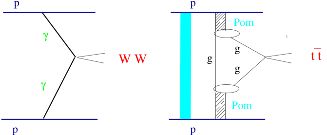
Figure 1: $\mathrm{W^{+}W^{-}}$ (QED) and $\mathrm{t\bar{t}}$ (QCD) exclusive production. Left: double photon exchange process. Right: exclusive double pomeron exchange in the Bialas-Landshoff model via “gluons in the pomeron”; The grey band represents the rapidity gap survival suppression factor (see text).

II.1 $\mathrm{W^{+}W^{-}}$ production via double photon exchange

The QED process rates are obtained from the following cross section formula

$$d\sigma_{(\mathrm{pp\to\ p\ W^{+}W^{-}p})}=\hat{\sigma}_{\mathrm{\gamma\gamma\to W^{+}W^{-}}}\ dn^{\gamma}_{1}\ dn^{\gamma}_{2}\ ,$$

where the Born $\mathrm{\gamma\gamma\to W^{+}W^{-}}$ cross-section reads Papageorgiu:1990mu

$$\hat{\sigma}_{\mathrm{\gamma\gamma\to W^{+}W^{-}}}=\frac{8\pi\alpha^{2}}{M_{\mathrm{WW}}^{2}}\left\{\frac{1}{t}\left(1+\frac{3}{4}t+3t^{2}\right)\Lambda-3t(1-2t)\ln\left(\frac{1+\Lambda}{1-\Lambda}\right)\right\},$$ (1)

with

$$t=\frac{m_{\mathrm{W}}^{2}}{M_{\mathrm{WW}}^{2}}\ ,\ \ \ \ \ \ \ \ \ \ \Lambda=\sqrt{1-4t}\ ,$$ (2)

where $M_{\mathrm{WW}}$ is the total $\mathrm{W^{+}W^{-}}$ mass. The photon fluxes $dn^{\gamma}$ are given by Budnev:1975zs

$$dn^{\gamma}=\frac{\alpha}{\pi}\frac{\omega}{\omega}\left(1-\frac{\omega}{E}\right)\left[\phi\left(\frac{q^{2}_{max}}{q^{2}_{0}}\right)-\phi\left(\frac{q^{2}_{min}}{q^{2}_{0}}\right)\right]\ ,$$ (3)

where

$$\phi\left(x\right)\equiv(1+ay)\left[\ln\left(\frac{x}{1+x}\right)+\Sigma_{k=1}^{3}\frac{1}{k(1+x)^{k}}\right]-\ \frac{(1-b)y}{4x(1+x)^{3}+c(1+\frac{1}{4}y)}\left[\ln\left(\frac{2+2x-b}{1+x}\right)+\Sigma_{k=1}^{3}\frac{b^{k}}{k(1+x)^{k}}\right]\ ,$$ (4)

and

$$q^{2}_{0}\sim 0.71\ \mathrm{GeV}^{2}\ \ ;\ y=\frac{\omega^{2}}{E(E-\omega)}\ \ ;\ a\sim 7.16\ \ ;\ b\ \ \sim-3.96\ \ ;\ c\sim 0.028\ ,$$ (5)

in the usual dipole approximation for the proton electromagnetic form factors. $\omega$ is the photon energy in the laboratory frame, $q^{2}$ the modulus of its mass squared in the range

$$\left[q^{2}_{min},\ q^{2}_{max}\right]\equiv\left[\frac{m^{2}\omega^{2}}{E(E-\omega)}\ ,\frac{t_{max}}{q^{2}_{0}}\right]\ ,$$ (6)

where $E$ and $m$ are the energy and mass of the incident particle and $t_{max}\equiv({m_{\mathrm{W}}^{2}}/{M_{\mathrm{W}\mathrm{W}}^{2}})_{max}$ is defined by the experimental conditions.

The QED cross section $d\sigma(\mathrm{pp\to\ p\ W^{+}W^{-}p})$ is a theoretically clear prediction. One should take into account however, two sources of (probably mild) correction factors. One is due to the soft QCD initial state radiation between incident protons which could destroy the large rapidity gap of the QED process. It is present but much less pronounced than for the rapidity gap survival for a QCD hard process (see the discussion in the next subsections), thanks to the large impact parameter implied by the QED scattering. The second factor is the QCD $\mathrm{gg\to W^{+}W^{-}}$ exclusive production via higher order diagrams. This has been evaluated recently Binoth:2005ua for standard (non diffractive) production to give a $5\%$ correction factor. The similar calculation for the diffractive $\mathrm{W^{+}W^{-}}$ production by comparison with the QED process is outside the scope of our paper but deserves to be studied together with the “inclusive” background ($\mathrm{W^{+}W^{-}}$+hadrons) it could generate.

II.2 Exclusive diffractive production of $\mathrm{t\bar{t}}$ events

Let us introduce the model bi90 ; ourpap we shall use for describing exclusive $\mathrm{t\bar{t}}$ production in double diffractive production. This process is depicted in Fig. 1 (right).

In bi90 , the diffractive mechanism is based on two-gluon exchange between the two incoming protons. The soft pomeron is seen as a pair of gluons non-perturbatively coupled to the proton. One of the gluons is then coupled perturbatively to the hard process (either the Higgs boson, or the $\mathrm{t\bar{t}}$ pair, see Fig. 1), while the other one plays the rôle of a soft screening of colour, allowing for diffraction to occur. The corresponding cross-sections for $\mathrm{q\bar{q}}$ and Higgs boson production read:

$$d\sigma_{\mathrm{t\bar{t}}}^{exc}(s)=C_{\mathrm{q\bar{q}}}^{exc}\left(\frac{s}{M_{\mathrm{q\bar{q}}}^{2}}\right)^{2\epsilon}\delta^{(2)}\left(\sum_{i=1,2}(v_{i}+k_{i})\right)\prod_{i=1,2}d^{2}v_{i}d^{2}k_{i}d\eta_{i}\ \xi_{i}^{2\alpha^{\prime}v_{i}^{2}}\!\exp(-2\lambda_{\mathrm{t\bar{t}}}v_{i}^{2})\ {\hat{\sigma}_{\mathrm{t\bar{t}}}}\ ,$$ (7)

where the variables $v_{i}$ and $k_{i}$ respectively denote the transverse momenta of the outgoing protons and of top quarks, $\xi_{i}$ are the proton fractional momentum losses, and $\eta_{i}$ are the quark rapidities,

$$\hat{\sigma}_{\mathrm{t\bar{t}}}\equiv\frac{\pi}{24}\frac{d\sigma}{dt}=\frac{\rho(1-\rho)}{m_{T1}^{2}m_{T2}^{2}}\,\,,\,\,\rho=\frac{4m_{\mathrm{t}}^{2}}{M_{\mathrm{t\bar{t}}}^{2}}\$$ (8)

is the hard $\mathrm{gg\to t\bar{t}}$ cross-section.

In the model, the soft pomeron trajectory is taken from the standard Donnachie-Landshoff parametrisation pom , namely $\alpha(t)=1+\epsilon+\alpha^{\prime}t$, with $\epsilon\approx 0.08$ and $\alpha^{\prime}\approx 0.25\mathrm{GeV^{-2}}$. $\lambda_{\mathrm{t\bar{t}}}$ and the normalization $C^{exc}_{\mathrm{t\bar{t}}}$ are kept as in the original paper bi90 . Note that, in this model, the strong (non perturbative) coupling constant is fixed to a reference value $G^{2}/4\pi=1,$ reflecting the lack of knowledge of the absolute normalization of exclusive DPE processes.

II.3 Inclusive diffractive production of $\mathrm{t\bar{t}}$ events

It is convenient to introduce also the model for central inclusive diffractive production BPR applied to $\mathrm{t\bar{t}}$ dijets. One writes

$$d\sigma_{\mathrm{t\bar{t}}}^{incl}=C_{\mathrm{t\bar{t}}}\left(\frac{x^{g}_{1}x^{g}_{2}s}{M_{\mathrm{t\bar{t}}}^{2}}\right)^{2\epsilon}\!\!\!\!\delta^{(2)}\!\left(\sum_{i=1,2}v_{i}\!+\!k_{i}\right)\prod_{i=1,2}\!\!\left\{{d\xi_{i}}{dx_{i}^{g}}d^{2}v_{i}d^{2}k_{i}{\xi_{i}}^{2\alpha^{\prime}v_{i}^{2}}\!\exp\left(-2v_{i}^{2}\lambda_{\mathrm{t\bar{t}}}\right)\right\}\ {\sigma_{\mathrm{t\bar{t}}}}\ G_{P}(x^{g}_{1},\mu)G_{P}(x^{g}_{2},\mu)\ .$$ (9)

In the above, $x_{i}^{g}$ are the pomeron’s momentum fractions carried by the gluons or quarks involved in the hard process, and the $G_{P}$ is the gluon energy density in the pomeron, $i.e.$, the gluon density multiplied by $x_{i}^{g}$. We use as parameterisations of the pomeron structure functions the fits to the diffractive HERA data performed in ba00 . The normalization $C_{\mathrm{t\bar{t}}}$ is obtained from the description BPR of the jet-jet diffractive cross-section at the Tevatron cdf . The hard cross-section ${\sigma_{\mathrm{t\bar{t}}}}$ to be considered is now

$${\sigma}_{\mathrm{t\bar{t}}}=\frac{\rho}{{(m^{\mathrm{t}}_{T1}})^{2}\ {(m^{\mathrm{t}}_{T2}})^{2}}\left(1-\frac{\rho}{2}\right)\left(1-\frac{9\rho}{16}\right)\ ,$$ (10)

to be distinguished from $\hat{\sigma}_{\mathrm{t\bar{t}}}$ (8) due to inclusive characteristics BPR .

II.4 Rapidity Gap Survival

In order to select exclusive diffractive states, such as for $\mathrm{W^{+}W^{-}}$ (QED) and ${\mathrm{t\bar{t}}}$ (exclusive, QCD), it is required to take into account the corrections from soft hadronic scattering. Indeed, the soft scattering between incident particles tends to mask the genuine hard diffractive interactions at hadronic colliders. The formulation of this correction sp to the scattering amplitude ${\cal A}_{(\mathrm{WW},\mathrm{t\bar{t}})}$ consists in considering a gap survival probability ($SP$) function $S$ such that

$${\cal A}(p_{T1},p_{T2},\Delta\Phi)=\left\{1+{\cal A}_{SP}\right\}{\bf\times}{\cal A}_{(\mathrm{WW},\mathrm{t\bar{t}})}\equiv{\cal S}{\bf\times}{\cal A}_{(\mathrm{WW},\mathrm{t\bar{t}})}=\int d^{2}{\bf k}_{T}\ {\cal S}({\bf k}_{T})\ {\cal A}_{(\mathrm{WW},\mathrm{t\bar{t}})}({\bf p}_{T1}\!-\!{\bf k}_{T},{\bf p}_{T2}\!+\!{\bf k}_{T})\ ,$$ (11)

where ${\bf p}_{T1,2}$ are the transverse momenta of the outgoing $p,\bar{p}$ and $\Delta\Phi$ their azimuthal angle separation. ${\cal A}_{SP}$ is the soft scattering amplitude.

The correction for the QED process is present but much less pronounced than for the rapidity gap survival for a QCD hard process, thanks to the large impact parameter implied by the QED scattering. In a specific model Khoze:2001xm the correction factor has been evaluated to be of order $0.9$ at the LHC for $\gamma\gamma\to\mathrm{H}.$ It is evaluated to be of order $0.03$ for the QCD exclusive diffractive processes at the LHC.

III Experimental context

III.1 The DPEMC Monte Carlo

A recently developed Monte-Carlo program, DPEMC dpemc , provides an implementation of the $\mathrm{W^{+}W^{-}}$ and $\mathrm{t\bar{t}}$ events described above in the QED and both exclusive and inclusive double pomeron exchange modes. It uses HERWIG herwig as a cross-section library of hard QCD processes, and when required, convolutes them with the relevant pomeron fluxes and parton densities. The survival probabilities discussed in the previous section (respectively 0.9 for double photon and 0.03 for double pomeron exchange processes) have been introduced at the generator level. The cross section at the generator level for $\mathrm{W^{+}W^{-}}$ QED and exclusive diffractive $\mathrm{t\bar{t}}$ production is found to be 55.9 fb and 40.1 fb for a $m_{\mathrm{W}}$ mass of 80.42 GeV and a top mass of 174.3 GeV after applying the survival probabilities.

III.2 Roman pot detector positions and resolutions

A possible experimental setup for forward proton detection is described in detail in helsinki . We will only describe its main features here and discuss its relevance for the $\mathrm{W}$ boson and top quark masses measurements.

In exclusive DPE or QED processes, the mass of the central heavy object can be reconstructed using the roman pot detectors and tagging both protons in the final state at the LHC. It is given by $M^{2}=\xi_{1}\xi_{2}s$, where $\xi_{i}$ are the proton fractional momentum losses, and $s$ the total center-of-mass energy squared. In order to reconstruct objects with masses in the 160 GeV range (for $\mathrm{W^{+}W^{-}}$ events) in this way, the acceptance should be large down to $\xi$ values as low as a few $10^{-3}$. For $\mathrm{t\bar{t}}$ events, an acceptance down to $10^{-2}$ is needed. The missing mass resolution directly depends on the resolution on $\xi$, and should not exceed a few percent to obtain a good mass resolution.

These goals can be achieved if one assumes two detector stations, located at $\sim 210$ m, and $\sim 420$ m helsinki from the interaction point. The $\xi$ acceptance and resolution have been derived for each device using a complete simulation of the LHC beam parameters. The combined $\xi$ acceptance is close to $\sim 60\%$ at low masses (at about twice $m_{\mathrm{W}}$), and 90% at higher masses starting at about 220 GeV. for $\xi$ ranging from $0.002$ to $0.1$. The acceptance limit of the device closest to the interaction point is $\xi>\xi_{min}=$0.02. Let us note also that the acceptance for $\mathrm{t\bar{t}}$ events goes down to 20% if only roman pots at 210 m are present since most of the events are asymmetric (one tag at 420m and another one at 210m).

Our analysis does not assume any particular value for the $\xi$ resolution. We will discuss in the following how the resolution on the $\mathrm{W}$ boson or the top quark masses depend on the detector resolutions, or in other words, the missing mass resolution.

III.3 Experimental cuts

This section summarises the cuts applied in the remaining part of the analysis. As said before, both diffracted protons are required to be detected in roman pot detectors.

The triggers which will be used for the $\mathrm{W^{+}W^{-}}$ and $\mathrm{t\bar{t}}$ events will be the usual ones at the LHC requiring in addition a positive tagging in the roman pot detectors.

The experimental offline cuts and their efficiencies have been obtained using a fast simulation of the CMS detector cmsim as an example, the fast simulation of the ATLAS detector leading to the same results. If we require at least one lepton (electron or muon) with a transverse momentum greater than 20 GeV and one (two) jet with a transverse momentum greater than 20 GeV (40 GeV) for $\mathrm{W^{+}W^{-}}$ ($\mathrm{t\bar{t}}$) to be reconstructed in the acceptance of the main detector in addition to the tagged protons , we get an efficiency of about 50% for $\mathrm{t\bar{t}}$ events, and 30% for $\mathrm{W^{+}W^{-}}$ events. We give the mass resolution as a function of luminosity in the following after taking into account these efficiencies. If the efficiencies are found to be higher, the luminosities have to be rescaled by this amount.

IV Threshold scan methods

IV.1 Explanation of the methods

We study two different methods to reconstruct the mass of heavy objects double diffractively produced at the LHC. As we mentioned before, the method is based on a fit to the turn-on point of the missing mass distribution at threshold.

One proposed method (the “histogram” method) corresponds to the comparison of the mass distribution in data with some reference distributions following a Monte Carlo simulation of the detector with different input masses corresponding to the data luminosity. As an example, we can produce a data sample for 100 fb^-1 with a top mass of 174 GeV, and a few MC samples corresponding to top masses between 150 and 200 GeV by steps of. For each Monte Carlo sample, a $\chi^{2}$ value corresponding to the population difference in each bin between data and MC is computed. The mass point where the $\chi^{2}$ is minimum corresponds to the mass of the produced object in data. This method has the advantage of being easy but requires a good simulation of the detector.

The other proposed method (the “turn-on fit” method) is less sensitive to the MC simulation of the detectors. As mentioned earlier, the threshold scan is directly sensitive to the mass of the diffractively produced object (in the $\mathrm{W^{+}W^{-}}$ case for instance, it is sensitive to twice the $\mathrm{W}$ mass). The idea is thus to fit the turn-on point of the missing mass distribution which leads directly to the mass of the produced object, the $\mathrm{W}$ boson. Due to its robustness, this method is considered as the “default” one in the following.

To illustrate the principle of these methods and their achievements, we apply them to the $\mathrm{W}$ boson and the top quark mass measurements in the following, and present in detail the reaches at the LHC. They can be applied to other threshold scans as well.

IV.2 W mass measurement

In this section, we will first describe the result of the “turn-on fit” method to measure the $\mathrm{W}$ mass. As we mentioned earlier, the advantage of the $\mathrm{W^{+}W^{-}}$ processes is that they do not suffer from any theoretical uncertainties since this is a QED process. The W mass can be extracted by fitting a 4-parameter ‘turn-on’ curve to the threshold of the mass distribution (c.f. Ref. Abbiendi:2002ay ):

$${\cal F}=P_{1}\cdot\left(\left[{e^{-\frac{x-P_{2}}{P_{3}}}+1}\right]^{-1}+P_{4}\right).$$ (12)

$P_{1}$ is the amplitude, $P_{2}$ the inflexion point, $P_{3}$ the width of the turn-on curve, and $P_{4}$ is a vertical offset, $x$ being the missing mass. With a detector of perfect resolution, $P_{2}$ would be equal to twice the $\mathrm{W}$ mass. However, the finite roman pot resolution leads to a shift between $P_{2}$ and $2m_{\mathrm{W}}$ which has to be established using a MC simulation of the detector for different values of its resolution. This shift is only related to the method itself and does not correspond to any error in data. For each value of the $\mathrm{W}$ input mass in MC, one has to obtain the shift between the reconstructed mass ($P_{2}/2$) and the input mass, which we call in the following the calibration curve. It is assumed for simplicity that $P_{2}$ is a linear function of $m_{\mathrm{W}}$, which is a good approximation as we will see next. In order to determine the linear dependence between $P_{2}$ and $m_{\mathrm{W}}$, calibration curves are calculated for several assumed resolutions of the roman pot detectors. The calibration points are obtained by fitting ${\cal F}$ to the mass distribution of high statistics samples (100 000 events) for several values of $m_{\mathrm{W}}$. An example is given in Fig. 2 for two resolutions of the roman pot detectors. The difference between the fitted values of $P_{2}/2$ and the input $\mathrm{W}$ masses are plotted as a function of the input W mass and are then fitted with a linear function. To minimise the errors on the slope and offset, the difference $P_{2}/2-80.42~{}\mbox{GeV}$ is plotted versus $m_{\mathrm{W}}$ (Fig. 3).

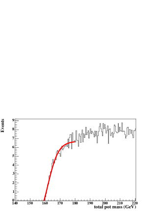
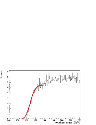
Figure 2: Two examples of fits to missing mass reference distributions with a resolution of the roman pot detectors of 1 GeV (left) and 3 GeV (right). We see on these plots the principle and the accuracy of the “turn-on fits” to the MC at threshold.

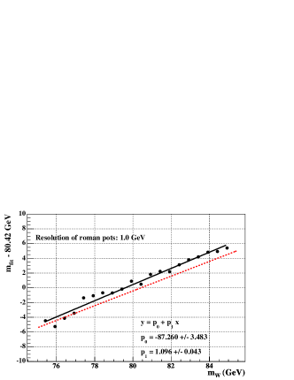
Figure 3: Calibration curves (see text) for two different roman pot resolutions of 1 GeV (left) and 3 GeV (right). We notice that the calibration can be fitted to a linear function with good accuracy. The dashed line indicates the first diagonal to show the shift clearly.

To evaluate the statistical uncertainty due to the method itself, we perform the fits with some 100 different “data” ensembles. For each ensemble, one obtains a different reconstructed $\mathrm{W}$ mass, the dispersion corresponding only to statistical effects. The expected statistical uncertainty on the actual measurement of the W mass in data is thus estimated with these ensemble tests for several integrated luminosities and roman pot resolutions. Each ensemble contains a number of events that corresponds to the expected event yield for a given integrated luminosity, taking into account selection and acceptance efficiencies. The turn-on function ${\cal F}$ is fitted to each ensemble. Only the parameters $P_{1}$ and $P_{2}$ are allowed to float, $P_{3}$ and $P_{4}$ are fixed to the average values obtained from the fits for the calibration points.

In order to obtain the fitted estimate for the W mass, $m_{\mathrm{W}}^{\mathrm{fit}}$, in each ensemble, the fit value of $P_{2}$ is corrected with the calibration curve that corresponds to the roman pot resolution. For each resolution $m_{\mathrm{W}}^{\mathrm{fit}}$ is histogrammed as shown in Fig. 4. The distributions are fitted with a Gauss function where the width corresponds to the expected statistical uncertainty of the W mass measurement. Fig. 5 shows the expected precision as a function of the integrated luminosity for several roman pot resolutions. With 150 $\mathrm{fb^{-1}}$ the expected statistical uncertainty on $m_{\mathrm{W}}$ is about 0.65 GeV when a resolution of the roman pot detectors of 1 GeV can be reached. With 300 $\mathrm{fb^{-1}}$ the expected uncertainty on $m_{\mathrm{W}}$ decreases to about 0.3 GeV.

We notice of course that this method is not competitive to get a precise measurement of the $\mathrm{W}$ mass, which would require a resolution to be better than 30 MeV. However, this method can be used to align precisely the roman pot detectors for further measurements. A precision of 1 GeV (0.3 GeV) on the $\mathrm{W}$ mass leads directly to a relative resolution of 1.2% (0.4%) on $\xi$ using the missing mass method. This calibration will be needed, for instance, to measure the top mass as proposed in the next section.

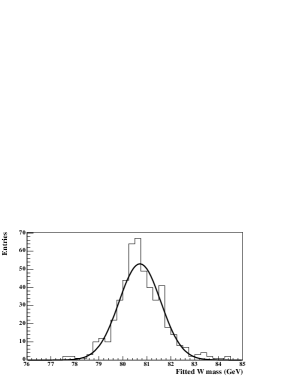
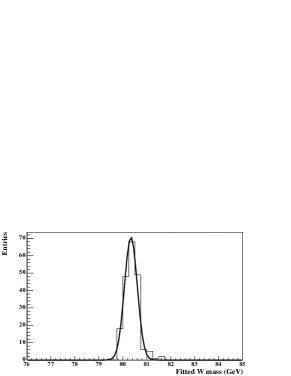
Figure 4: Distribution of the fitted value of the W mass from ensemble tests. Left: corresponding to 150 $\mathrm{fb^{-1}}$, right: corresponding to 300 $\mathrm{fb^{-1}}$. We note the resolution obtained on the $\mathrm{W}$ mass for these two luminosities.

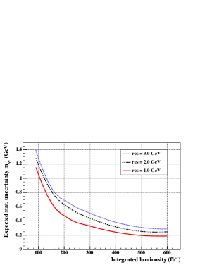
Figure 5: Expected statistical uncertainty on the $\mathrm{W}$ mass as a function of luminosity for three different roman pot resolutions.

Let us now present the result on the “histogram” method, which is an alternative approach to determine the W mass. The same high statistics templates used to derive the calibration curves are fitted directly to each ensemble (see Fig. 6 left). The $\chi^{2}$ is defined using the approximation of poissonian errors as given in Ref. Gehrels:1986mj . Each ensemble thus gives a $\chi^{2}$ curve which in the region of the minimum is fitted with a fourth-order polynomial (Fig. 6 right). The position of the minimum of the polynomial, $m_{\mathrm{W}}^{\mathrm{min}}$, gives the best value of the W mass and the uncertainty $\sigma(m_{\mathrm{W}})$ is obtained from the values where $\chi^{2}=\chi^{2}_{\text{min}}+1$. The mean value of $\sigma(m_{\mathrm{W}})$ for all ensembles are quoted as expected statistical uncertainties.

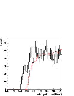
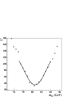
Figure 6: Left: Example of the histogram-fitting method. We see the difference between the “data” sample (full histogram with error bars, $m_{\mathrm{W}}=80.42~{}\mbox{GeV}$) and a reference histogram (dashed line, $m_{\mathrm{W}}=85.42~{}\mbox{GeV}$). Right: Example of the $\chi^{2}$ distribution in one ensemble.

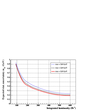
Figure 7: Expected statistical precision of the W mass as a function of the integrated luminosity for various resolutions of the roman pot detectors using the histogram-fitting method.

The expected statistical errors on the W mass using histogram fitting are comparable to those using the function fitting method. However, the former turns out to be more sensitive to the resolution of the roman pot detectors.

IV.3 Top mass measurement

The method to extract the top mass is the same as for the W mass described in the previous section. The theoretical cross section is not as well known as for the $\mathrm{W}$ and is model dependent. Our study assumes the Bialas Landshoff model for exclusive $\mathrm{t\bar{t}}$ production. For $\mathrm{t\bar{t}}$ events the width of the turn-on curve is considerably larger than for WW events (Fig. 8, left), resulting in a larger offset between the actual turn on and the inflexion point of the fit function. The calibration curve for a resolution of the roman pot detectors of 1 GeV is displayed in Fig. 8, right.

Ensemble tests for integrated luminosities of 50, 75, 100 and 200 fb^-1 and roman pot detector resolutions of 1 GeV, 2 GeV and 3 GeV yield the results shown in Fig. 9, left. Resolutions of the roman pot detectors between 1 GeV and 3 GeV give similar statistical uncertainties on the top quark mass which is due to the fact that the main limiting effect on resolution is statistics. With 100 $\mathrm{fb^{-1}}$ the expected statistical precision is about 1.6 GeV and gets improved to about 0.65 GeV with 300 $\mathrm{fb^{-1}}$.

The results have also been cross-checked using the histogram fitting method which was found to yield very similar expected uncertainties as the function fitting method (Fig. 9, right).

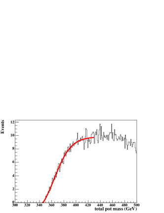
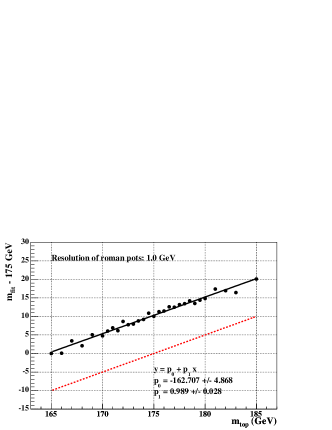
Figure 8: Fit to a reference mass distribution with $m_{\mathrm{t}}=175~{}\mbox{GeV}$ (left) and calibration curve for a roman pot resolution of 1 GeV, the diagonal is displayed in dashed line to show the difference (right). Note the larger difference between the calibration curve and the diagonal compared to the case of $\mathrm{W^{+}W^{-}}$ production.

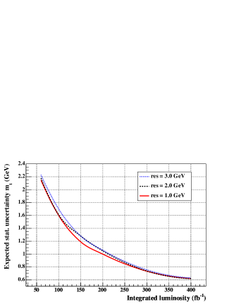
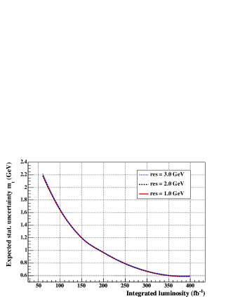
Figure 9: Expected statistical precision of the top mass as a function of the integrated luminosity for various resolutions of the roman pot detectors (full line: resolution of 1 GeV, dashed line: 2 GeV, dotted line: 3 GeV). Left: function fitting method, right: histogram fitting method (the three curves for different roman pot resolutions lead to the same results and cannot be distinguished in the figure).

V Outlook and prospects

In this section, we discuss other applications of the threshold scan method. Detailed analysis is postponed to forthcoming papers us .

As we mentioned before, the cross section of exclusive top pair production at the LHC is still uncertain, and predictions will be constrained by the incoming results form the Tevatron, especially from the DØ experiment where it is possible to detect double tagged events. On the contrary, inclusive double pomeron exchange has already been observed, and top quark pair production in this mode is fairly certain at the LHC. In this case, the threshold excitation is sensitive to quark and gluon densities at high pomeron momentum fraction, so that these events provide a rather unique opportunity to study structure functions near the endpoint.

Figure 10: Missing mass distributions at the generator level using the DPEMC Monte Carlo for the exclusive $\mathrm{t\bar{t}}$ events in full line and the results on inclusive $\mathrm{t\bar{t}}$ production for two different gluon densities in the pomeron (dashed line: fit 1, dotted line: fit 2, see Ref. h1 ).

Figure 11: Missing mass distributions at the generator level using the DPEMC Monte Carlo for the exclusive $\mathrm{t\bar{t}}$ events in full line, the inclusive events from model BPR ; ourpap (dashed line), and POMWIG (dotted line), see text.

To illustrate this point, we give in Fig. 10 the missing mass distributions at the generator level using the DPEMC Monte Carlo for the exclusive $\mathrm{t\bar{t}}$ events (full line) and the results on the Bialas-Landshoff inclusive $\mathrm{t\bar{t}}$ production for two different gluon densities in the pomeron (dashed line: fit 1, dotted line: fit 2, see Ref. h1 ). Fit 2 in Ref h1 leads to a more prominent gluon at high $\beta$ than fit 1. We see that the missing mass distribution is directly sensitive to the parton distributions in the pomeron. In Fig. 11, we display the differences between the exclusive $\mathrm{t\bar{t}}$ events in full line and the result of the factorisable POMWIG model (dotted line), and the non factorisable one based on the Bialas-Landshoff approach. We see again that the missing mass distribution, and thus the threshold analysis can help distinguishing between the models.

Another application of exclusive pair-production consists in measuring the mass of stops and sbottoms, provided these particles exist and can be produced in pairs at the LHC.

Finally, $\mathrm{W}$ pair-production in central diffraction gives access to the couplings of gauge bosons. Namely, as we mentioned already, $\mathrm{W^{+}W^{-}}$ production in two-photon exchange is robustly predicted within the Standard Model. Any anomalous coupling between the photon and the $\mathrm{W}$ will reveal itself in a modification of the production cross section, or by different angular distributions. Since the cross-section of this process is proportional to the fourth power of photon-$\mathrm{W}$ coupling, good sensitivity is expected.

VI Conclusion

Recent work on DPE has essentially focused on the Higgs boson search in the exclusive channel. In view of the difficulties and uncertainties affecting this search ourpap , we highlight new aspects of double diffraction which complement the diffractive program at the LHC.

In particular, QED W pair production provides a certain source of interesting diffractive events. Inclusive $\mathrm{t\bar{t}}$ production via double pomeron exchange is also an open channel and will provide interesting information on a poorly known aspect of structure functions. These robust channels will help and accompany the understanding of the more intriguing and challenging problem of exclusive double diffraction.

In this paper, we have advocated the interest of threshold scans in double pomeron exchange. This method considerably extends the physics program at the LHC. To illustrate its possibilities, we described in detail the $\mathrm{W}$ boson and the top quark mass measurements. The precision of the $\mathrm{W}$ mass measurement is not competitive with other methods, but provides a very precise calibration of the roman pot detectors. The precision of the top mass measurement is however competitive, with an expected precision better than 1 GeV at high luminosity. Other promising applications remain to be investigated.

References

- (1) M. G. Albrow and A. Rostovtsev [arXiv:hep-ph/0009336].
- (2) T. Affolder et al. [CDF Collaboration], Phys. Rev. Lett. 85, 4215 (2000).
- (3) M. Boonekamp, R. Peschanski and C. Royon, Phys. Rev. Lett. 87, 251806 (2001) [arXiv:hep-ph/0107113].
- (4) E. Papageorgiu, Phys. Lett. B 250, 155 (1990).
- (5) V. M. Budnev, A. N. Vall and V. V. Serebryakov, Yad. Fiz. 21, 1033 (1975).
- (6) T. Binoth, M. Ciccolini, N. Kauer and M. Kramer, arXiv:hep-ph/0503094.
- (7) A. Bialas and W. Szeremeta, Phys. Lett. B296 (1992) 191; A. Bialas and R. Janik, Zeit. für. Phys. C62 (1994) 487.
- (8) M. Boonekamp, R. Peschanski and C. Royon, Nucl. Phys. B 669, 277 (2003) [Erratum-ibid. B 676, 493 (2004)] [arXiv:hep-ph/0301244]; Phys. Lett. B 598, 243 (2004) [arXiv:hep-ph/0406061].
- (9) A. Donnachie, P. V. Landshoff, Phys. Lett. B207 (1988) 319.
- (10) C. Royon, L. Schoeffel, J. Bartels, H. Jung, R. Peschanski, Phys. Rev. D63 (2001) 074004.
- (11) J. D. Bjorken, Phys. Rev. D47, (1993) 101; E. Gotsman, E. Levin and U. Maor, Phys. Lett. B438 (1998), 229; A. B. Kaidalov, V. A. Khoze, A. D. Martin and M. G. Ryskin, Eur. Phys. J. C21 (2001) 521.
- (12) V. A. Khoze, A. D. Martin and M. G. Ryskin, Eur. Phys. J. C 23, 311 (2002) [arXiv:hep-ph/0111078].
- (13) M. Boonekamp, T. Kucs, Comput. Phys. Commun. 167 (2005) 217.
- (14) G. Corcella et al., JHEP 0101:010 (2001).
- (15) J. Kalliopuska, T. Mäki, N. Marola, R. Orava, K. Österberg, M. Ottela, HIP-2003-11/EXP.
-
(16)
CMSIM, fast simulation of the CMS detector, CMS Collab., Technical Design Report
(1997);
TOTEM Collab., Technical Design Report, CERN/LHCC/99-7;
ATLFAST, fast simulation of the ATLAS detector, ATLAS Collab, Technical Design Report, CERN/LHC C/99-14. - (17) G. Abbiendi et al. [OPAL Collaboration], Eur. Phys. J. C 26, 321 (2003) [arXiv:hep-ex/0203026].
- (18) N. Gehrels, Astrophys. J. 303, 336 (1986).
- (19) M. Boonekamp, J. Cammin, S. Lavignac, R. Peschanski, C. Royon, in preparation.
- (20) C. Royon, L. Schoeffel, J. Bartels, H. Jung, R. Peschanski, Phys.Rev. D63 (2001) 074004, a fit to the data from H1 Coll., Z. Phys. C76 (1997) 613. .
- (21) B. E. Cox and J. R. Forshaw, Comput. Phys. Commun. 144, 104 (2002) [arXiv:hep-ph/0010303].