Infrared enhanced analytic coupling and
chiral symmetry breaking in QCD

Abstract

We study the impact on chiral symmetry breaking of a recently developed model for the QCD analytic invariant charge. This charge contains no adjustable parameters, other than the QCD mass scale $\Lambda$, and embodies asymptotic freedom and infrared enhancement into a single expression. Its incorporation into the standard form of the quark gap equation gives rise to solutions for the dynamically generated mass that display a singular confining behaviour at the origin. Using the Pagels–Stokar method we relate the obtained solutions to the pion decay constant $f_{\pi}$, and estimate the scale parameter $\Lambda$, in the presence of four active quarks, to be about $880\,$MeV.

1 Introduction

The lack of a systematic calculational scheme applicable to the infrared sector of Quantum Chromodynamics (QCD) has motivated the advent of models aspiring to provide phenomenologically viable links between asymptotic freedom and confinement, by enriching perturbation theory with judiciously selected nonperturbative information. An important source of such information is provided by the dispersion relations. The latter, being based on the “first principles” of the theory, furnish the definite analytic properties with respect to a given kinematic variable of a physical quantity under consideration. The basic idea behind the so-called “analytic approach” to Quantum Field Theory (QFT) is to supplement perturbation theory, and in particular the renormalization group (RG) formalism, with the nonperturbative information encoded in the relevant dispersion relations. Specifically, the perturbative solutions of the RG equations possess unphysical singularities in the infrared domain, a fact that contradicts the general principles of local QFT. The analytization procedure amounts to the restoration of the correct analytic properties for a physical quantity at hand, by forcing it to satisfy the Källén–Lehmann spectral representation (see equation (1)). This method was first proposed in the framework of Quantum Electrodynamics (QED) and applied to the study of the invariant charge of the theory [1]. Later on, these considerations were generalized to the case of the non-Abelian theories, and the analytic approach to QCD [2] emerged. This approach has been successfully applied to the study of the strong running coupling [2, 3], perturbative series for the QCD observables [4], and some intrinsically nonperturbative aspects of the hadron dynamics [3, 5]. Some of the main advantages of the analytic approach to QCD are the absence of unphysical singularities (by construction), and a fairly good higher-loop and scheme stability of the results obtained.

A central quantity within the aforementioned approach is $\alpha(k^{2})$, the running (or “effective”) coupling (charge) of QCD. Clearly, this quantity can be reliably computed only in the ultraviolet region, where perturbation theory is applicable, and must be modelled in the infrared domain, where perturbative methods break down, and one eventually encounters the unphysical singularities, such as the Landau pole. The analytic approach to QCD eliminates such artefacts and provides a concrete analytic expression for the running coupling in the infrared, maintaining at the same time the standard asymptotic behaviour in the ultraviolet. However, since the analyticity requirement can be incorporated into the RG formalism in various ways, two main pictures have emerged. Specifically, if the analyticity condition is imposed directly on the perturbative running coupling $\alpha_{\mbox{\scriptsize s}}(k^{2})$ one arrives at the model of [2] with finite universal infrared limiting value given by $\alpha(0)=4\pi/\beta_{0}$. If, instead, the analyticity requirement is imposed on the corresponding $\beta$ function, one obtains the running coupling of [3] which is singular (“enhanced”) at $k^{2}=0$. The latter invariant charge has proved to be able to describe a number of the strong interaction processes both of perturbative and of nonperturbative nature [3, 5]. Undoubtedly, it would be interesting to further study the physical implications and phenomenological possibilities offered by the infrared enhanced analytic invariant charge. The primary objective of this paper is to examine the compatibility of the infrared enhanced analytic running coupling with chiral symmetry breaking (CSB), and its impact on the solutions of the Schwinger–Dyson (SD) equation controlling the dynamical generation of quark masses.

The way the running coupling enters into the standard SD equation for the quark propagator (“gap equation”) is rather well-known. Since QCD is not a fixed point theory, the QED–inspired gap equation must be modified, in order to incorporate the asymptotic freedom. The usual way of accomplishing this eventually boils down to the replacement $1/k^{2}\to\alpha(k^{2})/k^{2}$ in the corresponding kernel of the gap equation. The inclusion of $\alpha(k^{2})$ is essential for arriving at an integral equation for the quark propagator $S(p)$ which is well-behaved in the ultraviolet. Indeed, the additional logarithm in the denominator of the kernel due to the strong running coupling $\alpha(k^{2})$ improves the convergence of the integral. However, since the perturbative form of $\alpha(k^{2})$ diverges as $1/\ln(k^{2}/\Lambda^{2})$ when $k^{2}\to\Lambda^{2}$, a physically motivated model for the infrared behaviour of $\alpha(k^{2})$ is needed. The infrared enhanced analytic charge represents a good candidate for such a purpose, since, as has been explained in detail in [3, 5], it combines asymptotic freedom and confinement behaviour in a single expression. This is to be contrasted with the standard method of introducing asymptotic freedom and confinement (see, e.g., [6]), whereby the running coupling is composed by two separate, and theoretically rather uncorrelated, contributions (see further discussion in Section 4).

The paper is organized as follows. In Section 2 we briefly review the most salient features of the analytic approach, with particular emphasis on the running coupling displaying infrared enhancement. In Section 3 we go over the usual assumptions and approximations entering into the derivation of the standard gap equation. In Section 4 we study the asymptotic behaviour of the dynamical quark mass function, by converting the integral equation into a differential form. In Section 5 the integral equation is solved numerically, and the results are presented. It turns out that, with four active quarks, the experimental value of the pion decay constant $f_{\pi}$ may be obtained if the QCD mass-scale $\Lambda$, which is the only free parameter available, acquires the rather elevated value of about $880\,$MeV. Finally, in Section 6 we discuss the results and present our conclusions.

2 Analytic invariant charge in QCD

In this Section we give a brief summary of one of the models for the QCD analytic invariant charge [3]. This model shares all the advantages of the analytic approach and it was successful in the description of a wide range of QCD phenomena both of perturbative and of intrinsically nonperturbative nature [5]. Furthermore, it is of a particular interest to note that this model has recently been re-derived [7], proceeding from completely different motivations.

As has already been commented in the Introduction, the basic idea behind the analytic approach to QFT [1, 2] is to supplement perturbation theory with the nonperturbative information encoded in the relevant dispersion relations. The latter are based on “first principles” of the theory, and provide one with the definite analytic properties of a given physical quantity with respect to a proper kinematic variable. In practice the “analytization procedure” [2] amounts to the restoration of the correct analytic properties for a given quantity $F(k^{2})$ by imposing the Källén–Lehmann integral representation

$$\Bigl{\{}F(k^{2})\Bigr{\}}_{\mbox{$\!$\scriptsize an}}=\int_{0}^{\infty}\!\frac{\varrho(\sigma)}{\sigma+k^{2}}\,d\sigma.$$ (1)

Here the spectral function $\varrho(\sigma)$ is determined by the initial (perturbative) expression

$$\varrho(\sigma)=\frac{1}{2\pi i}\,\lim_{\varepsilon\to 0_{+}}\Bigl{[}F(-\sigma-i\varepsilon)-F(-\sigma+i\varepsilon)\Bigr{]},$$ (2)

with $\sigma>0$.

The model for the analytic invariant charge [3, 5] that we will study in this paper is obtained by imposing the requirement of analyticity (1) on the perturbative expansion of the RG $\beta$ function

$$\frac{d\,\ln\alpha^{(\ell)}_{\mbox{\scriptsize an}}(\mu^{2})}{d\,\ln\mu^{2}}=-\left\{\sum_{j=0}^{\ell-1}\beta_{j}\left[\frac{\alpha^{(\ell)}_{\mbox{\scriptsize s}}(\mu^{2})}{4\pi}\right]^{j+1}\right\}_{\mbox{\scriptsize$\!$an}}.$$ (3)

In this equation $\alpha^{(\ell)}_{\mbox{\scriptsize an}}(\mu^{2})$ is the $\ell$-loop analytic invariant charge, $\alpha^{(\ell)}_{\mbox{\scriptsize s}}(\mu^{2})$ denotes the $\ell$-loop perturbative running coupling, $\beta_{j}$ stands for the $\beta$ function expansion coefficient ($\beta_{0}=11-2n_{\mbox{\scriptsize f}}/3,\,$ $\beta_{1}=102-38n_{\mbox{\scriptsize f}}/3,\mbox{...}\,$), and $n_{\mbox{\scriptsize f}}$ is the number of active quarks. It is worth noting that prescription (3) differs from that of the original Shirkov–Solovtsov model [2], where the requirement (1) was imposed directly on the perturbative running coupling $\alpha_{\mbox{\scriptsize s}}(k^{2})$ (discussion of this issue can also be found in [3, 5, 8, 9]).

At the one-loop level the RG equation (3) can be solved explicitly [3]:

$$\alpha^{(1)}_{\mbox{\scriptsize an}}(k^{2})=\frac{4\pi}{\beta_{0}}\,\frac{z-1}{z\,\ln z},\qquad z=\frac{k^{2}}{\Lambda^{2}}.$$ (4)

The solution to equation (3) can also be represented in the form of the Källén–Lehmann integral

$$\alpha^{(\ell)}_{\mbox{\scriptsize an}}(k^{2})=\frac{4\pi}{\beta_{0}}\int_{0}^{\infty}\frac{\rho^{(\ell)}(\sigma)}{\sigma+z}\,d\sigma,$$ (5)

where the one-loop spectral density is

$$\rho^{(1)}(\sigma)=\left(1+\frac{1}{\sigma}\right)\frac{1}{\ln^{2}\!\sigma+\pi^{2}},$$ (6)

and the explicit expression for the $\ell$-loop $\rho^{(\ell)}(\sigma)$ can be found in [3, 5].

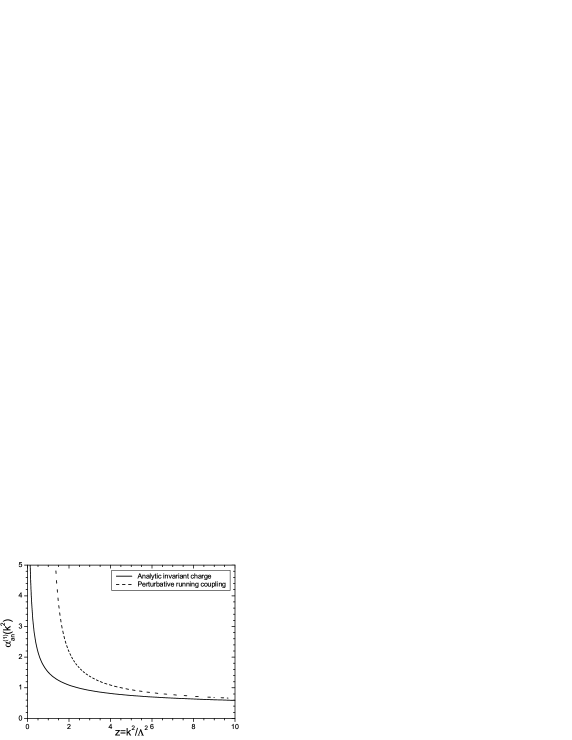
Figure 1: The analytic invariant charge $\alpha^{(1)}_{\mbox{\scriptsize an}}(k^{2})$ (see equation (4)) and the perturbative running coupling $\alpha^{(1)}_{\mbox{\scriptsize s}}(k^{2})$ at the one-loop level (solid and dashed curves, respectively). Here $n_{\mbox{\scriptsize f}}=4$ active quarks are assumed.

The invariant charge (4) possesses a number of appealing features. First of all, it has the correct analytic properties in the $k^{2}$ variable, demanded in equation (1), namely, it has the only cut $k^{2}\leq 0$ along the negative semiaxis of real $k^{2}$. Then, it contains no adjustable parameters. Thus, similarly to the perturbative approach, the QCD scale parameter $\Lambda$ remains the basic characterizing quantity of the theory. In addition, the invariant charge (4) incorporates the ultraviolet asymptotic freedom with the infrared enhancement in a single expression (see Figure 1), that plays an essential role in applications of the model in hand to the description of the quenched lattice simulation data (see [5, 7] for the details). It is worth mentioning here that the singular behaviour of the strong running coupling $\alpha(k^{2})$ when $k^{2}\to 0$ is also supported by a number of studies of the SD equations (see, e.g., papers [10, 11, 12, 13] and references therein). Moreover, the invariant charge (5) displays a good higher loop and scheme stability, and it has proved to describe a number of strong interaction processes (e.g., confining static quark–antiquark potential, inclusive $\tau$ lepton decay) in a self–consistent way. The detailed analysis of the properties of the analytic running coupling (5) and its applications can be found in [3, 5, 8].

Given the characteristic features of the analytic invariant charge mentioned above, it would be interesting to study its influence on phenomena particularly sensitive to the low-energy dynamics. To that end, in the following three sections we study how the analytic invariant charge (5) affects the the mechanism of CSB and dynamical mass generation for the quarks, through the study of the SD equations governing the dynamics of the quark propagator [14, 15, 16, 17, 18, 19, 20, 21, 22].

3 The gap equation

Throughout this Section, we will work exclusively in Euclidean space. According to the usual conventions, the starting point is to express the fully dressed quark propagator in the following general form [18]:

$$S^{-1}(p)=i/{p}+m_{0}+\Sigma(p)=i/{p}A(p^{2})+B(p^{2}),$$ (7)

where $m_{0}$ is the bare quark mass and $\Sigma(p)$ is the quark self-energy.

Before proceeding, it is worthwhile to make some additional comments on the above functions. Since we will be concentrated in the case where one does not have explicit CSB, i.e., the bare mass $m_{0}=0$, the quark mass is generated only through dynamical effects. In this case, CSB takes place when the self-energy $\Sigma(p)$ develops a nonzero value. Alternatively, one may define the quark mass function $M(p^{2})$ in terms of the functions $A(p^{2})$ and $B(p^{2})$, as $M(p^{2})=B(p^{2})/A(p^{2})$; then CSB is considered to occur when $B(p^{2})\neq 0$.

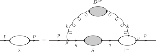
Figure 2: The SD equation (8) for the quark self-energy. The black blobs represent the fully dressed quark and gluon propagators and the white one is the proper quark-gluon vertex.

The quark SD equation is represented schematically in Figure 2 and can be written as

$$\Sigma(p)=\frac{4}{3}g^{2}\int\frac{d^{4}q}{(2\pi)^{4}}\gamma_{\mu}S(q)\Gamma_{\nu}(q,p)D^{\mu\nu}(k),$$ (8)

where we have used that $\sum_{a}\lambda^{a}\lambda^{a}=4/3$, $\lambda^{a}$ being the Gell-Mann matrices, and $k=p-q$. According to this equation, the self-energy $\Sigma(p)$ is dynamically determined in terms of itself, the full gluon propagator, denoted by $D_{\mu\nu}^{ab}(k)=\delta^{ab}D_{\mu\nu}(k)$, and the full quark-gluon vertex $\Gamma_{\nu}(q,p)$. Of course, both $D_{\mu\nu}^{ab}(k)$ and $\Gamma_{\nu}(q,p)$ obey their own complicated SD equations, a fact which eventually makes the use of simplifications unavoidable and further modelling of the unknown functions involved.

A common approximation employed in the literature (see, e.g., [10, 18, 23]) is to neglect the ghost contributions in the quark SD equation, whose effects are supposed to be partially accounted for by the fully dressed gluon propagator and the full quark-gluon vertex. This assumption leads to a theory with Abelian-like characteristics, where the usual non-Abelian Slavnov–Taylor identities are replaced by QED-like Ward identities [23]. In particular, for the quark-gluon vertex we have

$$i\,k^{\mu}\Gamma_{\mu}(p,q)=S^{-1}(p)-S^{-1}(q).$$ (9)

The imposition of this so-called “Abelian approximation” gives rise to further simplifications. Specifically, due to the (assumed) validity of equation (9), the usual QED identity $Z_{1}=Z_{2}$, where $Z_{1}$ and $Z_{2}$ are the renormalization constants for the fermion-boson vertex and fermion wave function, respectively, is restored. This, in turn, allows the definition of a RG invariant quantity, to be denoted by $\alpha(k^{2})$, which is the exact analogue of the QED effective charge, namely

$$g^{2}D_{\mu\nu}(k)=\left\{\delta_{\mu\nu}-\frac{k_{\mu}k_{\nu}}{k^{2}}\right\}\frac{4\pi\alpha(k^{2})}{k^{2}}.$$ (10)

The exact transversality of the right hand-side of equation (10) is the result of working in the Landau gauge. A different choice of gauge would have resulted in an additional longitudinal term of the form $\xi k_{\mu}k_{\nu}/k^{4}$, where $\xi$ is the usual gauge-fixing parameter ($\xi=0$ corresponds to the Landau gauge, $\xi=1$ to the Feynman gauge). Note that the nature of this extra term is purely tree-level, i.e., there is no higher-order dressing involved.

Furthermore, the Ward-identity (9) motivates the use of the time-honored “Gauge Technique” [24]. Specifically, a nonperturbative Ansatz for the vertex $\Gamma_{\mu}(p,q)$ in terms of $S(p)$ is postulated, based on the requirement that it should satisfy, by construction, equation (9). Evidently, such a construction leaves the transverse part of $\Gamma_{\mu}(p,q)$ unspecified; the usual argument around this ambiguity is that, in a theory with a mass-gap, the transverse parts of the vertex are sub-leading in the infrared, and have little or no consequence on CSB (see, e.g., [24]). In the rest of our analysis we will use for $\Gamma_{\mu}(p,q)$ the simple Ansatz proposed in [10, 23]

$$i\Gamma_{\mu}(p,q)=iA(p^{2})\gamma_{\mu}+\frac{k_{\mu}}{k^{2}}\left\{i\left[A(p^{2})-A(q^{2})\right]/{q}+\left[B(p^{2})-B(q^{2})\right]\right\}.$$ (11)

Choosing the Landau gauge leads to the further simplification

$$g^{2}D^{\mu\nu}(k)\Gamma_{\nu}(q,p)=g^{2}D^{\mu\nu}(k)A(q^{2})\gamma_{\nu},$$ (12)

since, in that case, the gluon propagator is completely transverse.

Substituting equations (7) and (12) into quark gap equation (8), one arrives at the commonly used coupled system for the quark self-energy [10, 18, 25]

$$\left[A(p^{2})-1\right]p^{2}=\frac{4}{3}\int\frac{d^{4}q}{(2\pi)^{4}}\frac{4\pi\alpha(k^{2})}{k^{2}}\left(p\!\cdot\!q+2\,\frac{p\!\cdot\!k\;q\!\cdot\!k}{k^{2}}\right)\frac{A^{2}(q^{2})}{q^{2}A^{2}(q^{2})+B^{2}(q^{2})}$$ (13)

and

$$B(p^{2})=4\int\frac{d^{4}q}{(2\pi)^{4}}\frac{4\pi\alpha(k^{2})}{k^{2}}\frac{A(q^{2})B(q^{2})}{q^{2}A^{2}(q^{2})+B^{2}(q^{2})}.$$ (14)

Note that the angular integration can be easily evaluated in the last two equations, by resorting to the usual angle approximation for the running coupling [10, 23, 26]

$$\alpha\left((p-q)^{2}\right)\approx\theta(p^{2}-q^{2})\alpha(p^{2})+\theta(q^{2}-p^{2})\alpha(q^{2}).$$ (15)

In particular, with such an approximation, the angular integral for the Dirac-vector component of the quark self-energy vanishes, leading automatically to $A(p^{2})=1$. Therefore, we can straightforwardly relate $B(p^{2})$ to the dynamical mass $M(p^{2})$. Then, the coupled system formed by equations (13) and (14), reduces to one single equation, namely [23]

$${\mathcal{M}}(x)=\frac{1}{\pi}\left[\frac{\alpha(x)}{x}\int_{0}^{x}\frac{y{\mathcal{M}}(y)}{y+{\mathcal{M}}^{2}(y)}dy+\int_{x}^{\infty}\frac{\alpha(y){\mathcal{M}}(y)}{y+{\mathcal{M}}^{2}(y)}dy\right],$$ (16)

where ${\mathcal{M}}(x)=M(x\Lambda^{2})/\Lambda$, $\,x=p^{2}/\Lambda^{2}$, and $y=q^{2}/\Lambda^{2}$.

4 Asymptotical behaviour of the mass function

The main effect of implementing the substitution described by equation (10) at the level of the gap equation is to transfer our ignorance regarding the behaviour of the gluon propagator into the nonperturbative structure of the invariant charge $\alpha(k^{2})$. This latter quantity can be modelled more directly, essentially because it enters more naturally than the gluon propagator in the parametrization of the low-energy QCD data. In the following sections, we will study in detail the solutions obtained from the quark gap equation (16) after using as $\alpha(k^{2})$ the one-loop analytic running coupling $\alpha^{(1)}_{\mbox{\scriptsize an}}(k^{2})$ (4).

The inclusion or not of appropriately modelled confinement effects has an important impact on the type of solutions that one obtains from the gap equation. In fact, it has often be claimed in the literature that, if such effects are not included, one may not encounter non-trivial solutions to the gap equation at all, i.e., CSB does not occur (see, e.g., [27]). The usual way of accounting for confinement effects at the level of the gap equation is to insert a gluon propagator of the form $\Lambda^{2}/k^{4}$, the (spacial) Fourier transform of linearly rising quark-antiquark potential [28]. Evidently, this expression fails to capture asymptotic freedom in the ultraviolet domain, whose effects are separately supplemented through the inclusion of the corresponding perturbative contributions. Thus, the “standard” way of describing both effects is through a running coupling of the form

$$\alpha_{\mbox{\scriptsize{\tiny KTW}}}(k^{2})=\frac{C}{z}+\frac{4\pi}{\beta_{0}}\frac{1}{\ln(z+\tau)},\qquad z=\frac{k^{2}}{\Lambda^{2}},$$ (17)

where $C$ and $\tau$ are dimensionless constants (see, e.g., [10]). Usually, $C$ is treated as an adjustable parameter, to be determined in such a way as to reproduce the correct phenomenological values for the quark masses, pion decay constant, and chiral condensates. On the other hand, $\tau$ plays the role of an infrared regulator; it is often treated as an arbitrary parameter, but in a more complete, physically motivated picture of QCD, it has been identified as a dynamically generated gluon “mass” [27, 29, 30]. Note that, if $C=0$, the logarithmic term on the right hand-side of (17) must overcome comfortably an infrared critical coupling of about 1.2, in order to obtain from the gap equations phenomenologically interesting solutions. This may or may not be possible, depending on whether $\tau$ is considered as a free parameter, or if some physical arguments constrain its possible range of values, as is the case with the gluon “mass”.

A definite advantage of the analytic invariant charge $\alpha^{(1)}_{\mbox{\scriptsize an}}(k^{2})$ (4), compared to (17), is the simultaneous incorporation of asymptotic freedom and infrared enhancement into a single expression, of concrete theoretical origin, namely the analyticity properties of the theory. In particular, note that, unlike a coupling of the type given in (17), the running coupling (4) contains no adjustable parameters. This theoretically appealing feature, is, of course, much more restrictive when one handles phenomenologically relevant quantities. It is worth noting also that the enhancement displayed by the analytic coupling $\alpha^{(1)}_{\mbox{\scriptsize an}}(k^{2})$ has been shown to correspond to the confining static quark-antiquark potential with a quasilinear rising behaviour at large distances. Namely, $V(r)\simeq r/\ln r$, when $r\to\infty$, with $r$ being the dimensionless distance between quark and antiquark, see [3, 5] for the details.

Before proceeding with the numerical solution for the SD equation (16) for all range of momenta, it would be interesting to gain some explicit insight into its behaviour in the deep infrared region. On general grounds, given that the running coupling (4) diverges at the origin, one might also expect a similar behaviour from the solutions of equation (16). In fact, this is what happens when (16) is solved using the running coupling (17), which is also singular in the infrared limit [10].

In order to obtain the low-energy asymptotic behaviour of the dynamical mass function ${\mathcal{M}}(x)$, it is convenient to cast the integral equation (16) into a differential form, by differentiating both sides twice with respect to $x$ (see also [10, 23])

$$\frac{d}{dx}\left[\frac{\frac{d}{dx}\left[\frac{x{\mathcal{M}}(x)}{\alpha(x)}\right]}{\frac{d}{dx}\left[\frac{x}{\alpha(x)}\right]}\right]=-\frac{1}{\pi}\frac{\alpha(x){\mathcal{M}}(x)}{x+{\mathcal{M}}^{2}(x)}.$$ (18)

By making use of the explicit form of the one-loop analytic invariant charge (4) one can reduce this equation in the limit $x\to 0$ to

$${\mathcal{M}}(v)\left(\frac{d^{2}}{dv^{2}}+2\frac{d}{dv}\right){\mathcal{M}}(v)=\frac{8}{\beta_{0}v}\,,\qquad v\to-\infty,$$ (19)

where $v=\ln x$. In deriving (19) we have neglected the factor $z$ in the numerator of (4), since in the limit considered it is subleading next to $1$. The above equation can be solved analytically through successive iterations, giving rise, as expected, to divergent solutions, which are formally expressed in terms of powers of $v$ and $\ln v$. The first iteration, corresponding to the leading infrared behaviour of the dynamical mass function ${\mathcal{M}}(x)$, is obtained by omitting the second-order derivative in equation (19). Then, the solution is

$${\mathcal{M}}(x)\simeq\sqrt{\frac{8}{\beta_{0}}\ln|\ln x|},\qquad x\to 0.$$ (20)

The divergence of the dynamical quark mass function ${\mathcal{M}}(x)$ in the low-energy domain $x\to 0$ can be interpreted as a hint for confinement, see also discussion in [10, 31].

It is worthwhile to emphasize again that the obtained behaviour (20) is restricted to the deep infrared domain (i.e., for values $p^{2}\ll\Lambda^{2})$. Subleading corrections to this solution may be systematically obtained from equation (19); however, they are of the same order as the terms neglected when arriving from (18) to (19), and are therefore of little usefulness. It is also interesting to compare equation (20) to the corresponding solution obtained by making use of the running coupling (17). The leading low-energy behaviour in that case is instead ${\mathcal{M}}_{\mbox{\tiny KTW}}(x)\simeq\sqrt{2C|\ln x|/\pi}$, when $x\to 0$. Thus, we infer that for the case of the analytic invariant charge (4) the infrared singularity of the dynamical mass function ${\mathcal{M}}(x)$ is much milder than in the case of the running coupling (17).

For the sake of completeness, we finish this Section by reporting the ultraviolet asymptotic expression for the dynamical quark mass ${\mathcal{M}}(x)$. Since we are considering the case of exact chiral symmetry (i.e., no bare mass, $m_{0}=0$), the conservation of the axial-vector current eventually leads, for sufficient large momenta, to

$${\mathcal{M}}(x)\simeq\frac{D}{x}(\ln x)^{\lambda-1},\qquad x\to\infty,$$ (21)

where $\lambda=12/(33-2n_{\mbox{\scriptsize f}})$ is the anomalous dimension of the mass, and $D$ is a constant independent of the renormalization point and directly related to the quark condensate [32, 33].

5 Numerical solution for the mass function

The numerical solution for the dynamical quark mass function ${\mathcal{M}}(x)$, obtained solving directly the integral equation (16), is presented in Figure 3. Indeed, one can see numerically a soft increase of the mass function ${\mathcal{M}}(x)$ when $x\to 0$, as suggested by the leading behaviour (20) extracted from the differential equation analysis. Regarding the ultraviolet region, we note that choosing sufficiently large values for the ultraviolet cutoff, the results obtained are independent of the latter, since the integrals in equation (16) are ultraviolet convergent. Typically, our solutions are evaluated within a momenta window of sixteen orders of magnitude $(10^{-8}\leq x\leq 10^{8})$, which is sufficient to ensure their stability.

Figure 3: The dimensionless quark dynamical mass ${\mathcal{M}}(x)=M(x\Lambda^{2})/\Lambda$, obtained from equation (16) using the one-loop analytic invariant charge (4) for $n_{\mbox{\scriptsize f}}=4$ quark flavours.

Now, with the solution for the dynamical mass at hand, we can relate the value of the QCD scale parameter $\Lambda$ to the pion decay constant $f_{\pi}$, defined as the axial-vector transition amplitude for an on-shell pion. This can be accomplished by making use of the method developed by Pagels, Stokar [34], and Cornwall [31], which is a generalization of the Goldberger–Treiman relation when the momentum carried by the pion is different from zero:

$$f_{\pi}^{2}=\frac{3\Lambda^{2}}{4\pi^{2}}\int_{0}^{\infty}\frac{y{\mathcal{M}}(y)}{\left[y+{\mathcal{M}}^{2}(y)\right]^{2}}\left[{\mathcal{M}}(y)-\frac{y}{2}\frac{d{\mathcal{M}}(y)}{dy}\right]dy.$$ (22)

Thus, one is able to fix the value for $\Lambda$, the only adjustable parameter in this analysis, by requiring that the pion decay constant should assume its measured value of $f_{\pi}=93\,$MeV [35]. For the more favorable case of $n_{\mbox{\scriptsize f}}=4$ active quarks this procedure results in the estimate $\Lambda=880\,$MeV.

The inclusion of the higher loop corrections to the analytic running coupling $\alpha_{\mbox{\scriptsize an}}(k^{2})$ (see equation (5)) is not expected to alter the qualitative picture obtained above. This is so because the most intrinsic feature of this charge, namely the infrared enhancement, persists after the incorporation of the loop corrections; however, the type of singularity displayed at the origin becomes slightly milder than in the one-loop case. Therefore, we anticipate that the confining behaviour of ${\mathcal{M}}(x)$ will also persist, but with a weaker infrared singularity then that of equation (20). On the other hand, in this case one would expect a higher estimate for $\Lambda$, given that the loop corrections lower the value of $\alpha_{\mbox{\scriptsize an}}(k^{2})$ in the entire range of momenta [5]. This fact, in turn, will lead to smaller values for ${\mathcal{M}}(x)$, making the saturation of the right hand-side of (22) more difficult, and forcing $\Lambda$ to assume even higher values.

We finish this Section by commenting on the veracity of the angular approximation given in equation (15), and the dependence of the obtained results on it. It would be certainly of interest to establish whether the divergent nature of the solutions persists, or is an artefact of the aforementioned approximation. Indeed, one could envisage the possibility that the simultaneous solution of the system (13) and (14) might actually lead to a finite expression for ${\mathcal{M}}(x)$, as $x\to 0$, despite the fact that the kernel is divergent at the origin, due to the enhanced form of the running charge (4) employed. In order to address this point in some detail, we have not resorted to the approximation of equation (15), but have instead performed the angular integration numerically, and subsequently attempted to solve the resulting coupled system. The numerical integration of the final (momentum) integrals requires the introduction of an infrared regulator [36]; we have regulated the kernels by carrying out the replacement $\alpha(k^{2})/k^{2}\rightarrow\alpha(k^{2})/(k^{2}+\mu^{2})$. Evidently, the solutions for the dynamical mass function depend now explicitly on the regulator $\mu$, and one should study the behaviour of ${\mathcal{M}}(x,\mu^{2})$ in the limit $\mu^{2}\to 0$. Our numerical analysis revealed that there is a critical value of $\mu^{2}$, of about $\mu^{2}\simeq 10^{-7}\Lambda^{2}$, below which no convergent solutions to the system (13) and (14) may be found. Although no inescapable conclusion may be drawn from this fact, we interpret this breakdown as a strong indication that the resulting solutions diverge as $\mu^{2}\to 0$, in qualitative agreement with what was found when the angular approximation of equation (15) was used.

6 Conclusions

In this paper we have studied the compatibility between the infrared enhanced analytic charge of QCD and chiral symmetry breaking, through the detailed analysis of a standard form of the gap equation for the quark propagator, where this former coupling was incorporated. It turned out that, due to the infrared enhancement of the running coupling employed, the solutions found for the dynamical quark mass function $M(p^{2})$ were infrared divergent. Following standard arguments we have interpreted this divergent behaviour as an indication of confinement. The final upshot of this analysis was that the aforementioned analytic charge is able to break the chiral symmetry, furnishing a reasonable ratio between the QCD scale parameter $\Lambda$ and the pion decay constant $f_{\pi}$.

To be sure, the value of 880 MeV obtained for $\Lambda$ (with four active quark flavours) appears elevated when compared to the “standard” value of $\Lambda$ of about 350 MeV quoted in the literature (see [35] and references therein), but also when compared to the values for $\Lambda$ obtained within the analytic approach itself by resorting to different methods [5], ranging between 500-600 MeV. We emphasize, however, that the main purpose of the analysis presented is not so much to extract an accurate value for $\Lambda$, but rather check to what extend two a priori different methods, the analytic approach and the SD equations, may coexist in a complementary and qualitatively consistent picture. In that sense we consider the outcome of the present work encouraging, especially when taking into account the theoretical uncertainties intrinsic to both methods, and the fact that, unlike the majority of existing models, in our case $\Lambda$ is the only adjustable parameter available.

It would certainly be worthwhile attempting to improve the above picture by incorporating into the spectral density defining the analytic charge (see equation (5)) contributions from nonperturbative effects (e.g., the operator product expansion (see also [38]) and the nonlocal chiral quark model [39]). We hope to be able to report progress in this direction in the near future.

References

References

- [1] P.J. Redmond, Phys. Rev. 112, 1404 (1958); P.J. Redmond and J.L. Uretsky, Phys. Rev. Lett. 1, 147 (1958); N.N. Bogoliubov, A.A. Logunov, and D.V. Shirkov, Zh. Eksp. Teor. Fiz. 37, 805 (1959) [Sov. Phys. JETP 37, 574 (1960)].
- [2] D.V. Shirkov and I.L. Solovtsov, Phys. Rev. Lett. 79, 1209 (1997).
- [3] A.V. Nesterenko, Phys. Rev. D 62, 094028 (2000); 64, 116009 (2001).
- [4] D.V. Shirkov, Teor. Mat. Fiz. 119, 55 (1999) [Theor. Math. Phys. 119, 438 (1999)]; Eur. Phys. J. C 22, 331 (2001); I.L. Solovtsov and D.V. Shirkov, Teor. Mat. Fiz. 120, 482 (1999) [Theor. Math. Phys. 120, 1220 (1999)].
- [5] A.V. Nesterenko, Nucl. Phys. B (Proc. Suppl.) 133, 59 (2004); Int. J. Mod. Phys. A 18, 5475 (2003).
- [6] W. Celmaster and F.S. Henyey, Phys. Rev. D 18, 1688 (1978); R. Levine and Y. Tomozawa, ibid. D 19, 1572 (1979); J.L. Richardson, Phys. Lett. B 82, 272 (1979); W. Buchmuller, G. Grunberg, and S.-H.H. Tye, Phys. Rev. Lett. 45, 103 (1980); 45, 587(E) (1980); W. Buchmuller and S.-H.H. Tye, Phys. Rev. D 24, 132 (1981).
- [7] F. Schrempp, J. Phys. G 28, 915 (2002).
- [8] A.V. Nesterenko, Mod. Phys. Lett. A 15, 2401 (2000); A.V. Nesterenko and I.L. Solovtsov, ibid. A 16, 2517 (2001).
- [9] D.V. Shirkov, Teor. Mat. Fiz. 132, 484 (2002) [Theor. Math. Phys. 132, 1309 (2002)]; arXiv:hep-ph/0408272.
- [10] G. Krein, P. Tang, and A.G. Williams, Phys. Lett. B 215, 145 (1988).
- [11] M. Baker, J.S. Ball, and F. Zachariasen, Nucl. Phys. B 186, 531 (1981); 186, 560 (1981); S. Mandelstam, Phys. Rev. D 20, 3223 (1979); N. Brown and M.R. Pennington, ibid. D 38, 2266 (1988); 39, 2723 (1989).
- [12] A.I. Alekseev and B.A. Arbuzov, Mod. Phys. Lett. A 13, 1747 (1998); A.I. Alekseev, arXiv:hep-ph/0503242.
- [13] V.S. Gogohia, Int. J. Mod. Phys. A 9, 759 (1994).
- [14] V.A. Miransky, V.P. Gusynin, and Yu.A. Sitenko, Phys. Lett. B 100, 157 (1981); V.A. Miransky and P.I. Fomin, ibid. B 105, 387 (1981); P.I. Fomin, V.P. Gusynin, V.A. Miransky, and Yu.A. Sitenko, Riv. Nuovo Cimento 6, 1 (1983).
- [15] K. Higashijima, Phys. Rev. D 29, 1228 (1984).
- [16] H. Pagels, Phys. Rev. D 19, 3038 (1979).
- [17] J.M. Cornwall, R. Jackiw, and E. Tomboulis, Phys. Rev. D 10, 2428 (1974).
- [18] C.D. Roberts and A.G. Williams, Prog. Part. Nucl. Phys. 33, 477 (1994).
- [19] R. Alkofer and L. von Smekal, Phys. Rept. 353, 281 (2001).
- [20] V. Sauli, arXiv:hep-ph/0410167; arXiv:hep-ph/0412188.
- [21] D. Kekez and D. Klabucar, Fizika B 13, 461 (2004).
- [22] M. Hashimoto and M. Tanabashi, arXiv:hep-ph/0210115.
- [23] D. Atkinson and P.W. Johnson, Phys. Rev. D 37, 2290 (1988); 37, 2296 (1988); D. Atkinson, P.W. Johnson, and K. Stam, ibid. D 37, 2996 (1988).
- [24] A. Salam, Phys. Rev. 130, 1287 (1963); A. Salam and R. Delbourgo, ibid. 135, 1398 (1964); R. Delbourgo and P. West, J. Phys. A 10, 1049 (1977); Phys. Lett. B 72, 96 (1977); R. Delbourgo and R.B. Zhang, J. Phys. A 17, 3593 (1984).
- [25] A.A. Natale and P.S. Rodrigues da Silva, Phys. Lett. B 390, 378 (1997); 392, 444 (1997).
- [26] A.C. Aguilar, A.A. Natale, and R. Rosenfeld, Phys. Rev. D 62, 094014 (2000).
- [27] J. Papavassiliou and J.M. Cornwall, Phys. Rev. D 44, 1285 (1991).
- [28] G.B. West, Phys. Lett. B 115, 468 (1982).
- [29] J.M. Cornwall, Phys. Rev. D 26, 1453 (1982).
- [30] J.M. Cornwall and J. Papavassiliou, Phys. Rev. D 40, 3474 (1989).
- [31] J.M. Cornwall, Phys. Rev. D 22, 1452 (1980).
- [32] V.A. Miransky, Phys. Lett. B 165, 401 (1985); 248, 151 (1990).
- [33] H.D. Politzer, Nucl. Phys. B 117, 397 (1976); Phys. Lett. B 116, 171 (1982).
- [34] H. Pagels and S. Stokar, Phys. Rev. D 20, 2947 (1979).
- [35] S. Eidelman et al. (Particle Data Group), Phys. Lett. B 592, 1 (2004).
- [36] A.G. Williams, G. Krein, and C.D. Roberts, Annals Phys. 210, 464 (1991).
- [37] G. Fogleman, D.B. Lichtenberg, and J.G. Wills, Lett. Nuovo Cim. 26, 369 (1979).
- [38] D.M. Howe and C.J. Maxwell, Phys. Rev. D 70, 014002 (2004).
- [39] A.E. Dorokhov and W. Broniowski, Eur. Phys. J. C 32, 79 (2003); I.V. Anikin, A.E. Dorokhov, and L. Tomio, Fiz. Elem. Chast. Atom. Yadra 31, 1023 (2000) [Phys. Part. Nucl. 31, 509 (2000)]; A.E. Dorokhov, Phys. Rev. D 70, 094011 (2004).