PITHA 05/04

Freiburg-THEP 05/03

ZU-TH 05/05

hep-ph/0504190

Two-Loop QCD Corrections to the Heavy Quark
Form Factors: Anomaly Contributions
W. Bernreuther$\rm\,{}^{a,\,}$, R. Bonciani$\rm\,{}^{b,\,}$, T. Gehrmann$\rm\,{}^{c,\,}$,

R. Heinesch$\rm\,{}^{a,\,}$, T. Leineweber$\rm\,{}^{a,\,}$ and E. Remiddi$\rm\,{}^{d,\,}$
^a Institut für Theoretische Physik, RWTH Aachen, D-52056 Aachen, Germany ^b Fakultät für Mathematik und Physik, Albert-Ludwigs-Universität Freiburg,
D-79104 Freiburg, Germany ^c Institut für Theoretische Physik, Universität Zürich, CH-8057 Zürich, Switzerland ^d Dipartimento di Fisica dell’Università di Bologna, and INFN, Sezione di Bologna, I-40126 Bologna, Italy

We present closed analytic expressions for the order $\alpha_{s}^{2}$ triangle diagram contributions to the matrix elements of the singlet and non-singlet axial vector currents between the vacuum and a quark-antiquark state. We have calculated these vertex functions for arbitrary momentum transfer and for four different sets of internal and external quark masses. We show that both the singlet and non-singlet vertex functions satisfy the correct chiral Ward identities. Using the exact expressions for the finite axial vector form factors, we check the quality and the convergence of expansions at production threshold and for asymptotic energies.

1 Introduction

This paper is the third of a series that deals with the computation of the electromagnetic and neutral current form factors of heavy quarks $Q$ at the two-loop level in QCD [1, 2]. Knowledge of these form factors puts forward the aim of a completely differential description of the electroproduction of heavy quarks, $e^{+}e^{-}\to\gamma^{*},Z^{*}\to Q{\bar{Q}}X$, to order $\alpha_{s}^{2}$ in the QCD coupling. This, in turn, will allow precise calculations or predictions of many observables, including forward-backward asymmetries, which are relevant for the (re)assessment of existing data on $b$ quark production at the $Z$ resonance [3], or which will become important for the production of $b$ quarks and $t$ quarks at a future linear collider [4]. A detailed list of references can be found in [1, 2].

In [1, 2] we presented analytic results to order $\alpha_{s}^{2}$ of the heavy quark vector and axial vector vertex form factors for arbitrary momentum transfer, up to anomalous contributions. Here we close this gap and analyze the triangle diagram contributions to the axial vector vertex which exhibit the Adler-Bell-Jackiw (ABJ) anomaly [5, 6]. We use dimensional regularization and the prescription of [7, 8] for implementing the Dirac matrix $\gamma_{5}$ in $D\neq 4$, which is an adaptation of the method of [9]. In Section 2 we set up the notation and discuss chiral Ward identities which must be satisfied by the appropriately renormalized axial vector current of a heavy quark, and the flavor-singlet and non-singlet axial vector currents, respectively. In Section 3 we give closed analytic expressions to order $\alpha_{s}^{2}$ for the anomalous (pure singlet) contributions to the axial vector form factors for four different sets of internal and external quark masses. First we present our results for spacelike squared momentum transfer $s$; then the form factors are analytically continued into the timelike region, and we determine also their threshold and asymptotic expansions. We check that the form factors satisfy the chiral Ward identities discussed in Section 2. In the context of this check we have calculated also the triangle diagram contributions to the pseudoscalar vertex function and the vertex function of the gluonic operator $G\tilde{G}$. In [10] the triangle contributions to the $b\bar{b}$ vertex function of the non-singlet current ${\bar{t}}\gamma_{\mu}\gamma_{5}t-{\bar{b}}\gamma_{\mu}\gamma_{5}b$ were computed for massless $b$ quarks, using the method of dispersion relations. Our chirality-conserving form factors for this specific mass combination confirm that result. In Section 4, we expand our exact expressions for the finite axial vector form factors at the production threshold and at asymptotic energies. Detailed comparison of this expansions with the full result allows us to assess the convergence properties of these widely used expansion techniques [11, 12]. We conclude in Section 5.

2 Chiral Ward Identities

We consider QCD with $N_{f}-1$ massless and one massive quark. This includes the case of $N_{f}=6$ with all quarks but the top quark taken to be massless. We analyze the following external currents:
$\bullet$ The currents $J_{5\mu}(x)={\bar{Q}}(x)\gamma_{\mu}\gamma_{5}Q(x)$ and $J_{5}={\bar{Q}}(x)\gamma_{5}Q(x)$, where $Q$ denotes the field associated with the massive quark. These currents are called axial vector and pseudoscalar current in what follows.
$\bullet$ The flavor-singlet axial vector current $J_{5\mu}^{S}(x)=\sum{\bar{q}}(x)\gamma_{\mu}\gamma_{5}q(x)$, where the sum extends over all quark flavors including $Q$.
$\bullet$ The flavor non-singlet neutral axial vector current $J_{5\mu}^{NS}=\sum_{i=1}^{3}{\bar{\psi}_{i}}\gamma_{\mu}\gamma_{5}\tau_{3}\psi_{i}$, where $\psi_{i}=(u,d)_{i}$ is the i-th generation quark isodoublet and $\tau_{3}$ is the 3rd Pauli matrix. This current couples to the $Z$ boson. The corresponding pseudoscalar current is denoted by $J_{5}^{NS}$.
The current $J_{5\mu}^{NS}$ is conserved in the limit of vanishing quark masses, while the currents $J_{5\mu}$ and $J_{5\mu}^{S}$ are anomalous at the quantum level [5, 6].

2.1 Axial Vector and Pseudoscalar Vertex Functions

In the following we study the matrix elements of the axial vector and pseudoscalar vertex functions between the vacuum and an on-shell $q\bar{q}$ pair to order $\alpha_{s}^{2}$ in the QCD coupling, where $q$ denotes one of the $N_{f}$ quark flavors. The bare 1-particle irreducible (1PI) vertex functions involving $J_{5\mu}$ and $J_{5}$ are denoted by $\Gamma_{q,\mu}$ and $\Gamma_{q}$, respectively. The kinematics is $J(p)\to q(p_{1})+{\bar{q}}(p_{2})$, with $p=p_{1}+p_{2}$:

$$\Gamma_{q,\mu}(s)=\gamma_{\mu}\gamma_{5}+\Lambda_{q,\mu}(s)\,,$$ (1)

$$\Gamma_{q}(s)=\gamma_{5}+\Lambda_{q}(s)\;.$$ (2)

Following [5] it is useful to distinguish between two types of contributions to $\Lambda_{q,\mu}$ and $\Lambda_{q}$ and, likewise, for the other vertex functions considered below: those where the axial vector (pseudoscalar) vertex $\gamma_{\mu}\gamma_{5}$ $(\gamma_{5})$ is attached to the external quark line $q$ are called type A. For the axial vector and pseudoscalar currents defined above these are non-zero only for $q=Q$. Type B contributions are called those where $\gamma_{\mu}\gamma_{5}$, respectively $\gamma_{5}$, is attached to a quark loop. To order $\alpha_{s}^{2}$ these are the triangle diagrams Fig. 1 (a) for the heavy quark currents $J_{5,\mu}$ and $J_{5}$, and the diagrams Figs. 1 (a,b) for $J^{S}_{5,\mu}$, $J^{S}_{5}$, $J^{NS}_{5,\mu}$, and $J^{NS}_{5}$. For massless quarks in the triangle Fig. 1 (b) only Fig. 1 (a) contributes to the matrix elements of $J_{5}^{S}$ and $J_{5}^{NS}$.

(40,25) i o1,o2 o1,o2 dashesvz,i phantomo1,v1,v2,v3,v4,vz,v5,v6,v7,v8,o2 dbl_plainvz,v3,v6,vz plaino1,v1,v8,o2 gluonv1,v3 gluonv6,v8 $\bar{q}(p_{2})$o1 $q(p_{1})$o2

(40,25) i o1,o2 o1,o2 dashesvz,i phantomo1,v1,v2,v3,v4,vz,v5,v6,v7,v8,o2 plainvz,v6,v3,vz plaino1,v1,v8,o2 gluonv1,v3 gluonv6,v8 $\bar{q}(p_{2})$o1 $q(p_{1})$o2

Figure 1: Triangle diagram (type B) contributions to the various axial vector and pseudoscalar vertex functions considered in this paper. The double and single straight line triangles in (a) and (b) denote massive and massless quarks, respectively. The external $q,\,\bar{q}$ quarks are either massive or massless. The dashed line denotes either an axial vector or a pseudoscalar vertex. The crossed diagrams are not drawn.

(40,25) i o1,o2 dotsi,v phantomo1,v1,v2,v3,v,v4,v5,v6,o2 plaino1,v1,v6,o2 gluonv1,v gluon,ruboutv,v6 v $\bar{q}(p_{2})$o1 $q(p_{1})$o2

Figure 2: One-loop anomalous vertex function $F_{q}$.

The anomalous Ward identities, which will be discussed in Section 2.3, involve also the truncated matrix element of the gluonic operator $G{\tilde{G}}$ between the vacuum and an on-shell $q\bar{q}$ pair. Here

$$G(x){\tilde{G}}(x)\equiv\epsilon_{\mu\nu\alpha\beta}G^{a,\mu\nu}(x)G^{a,\alpha\beta}(x)\;,$$ (3)

with $G^{a,\mu\nu}$ being the gluon field strength tensor. The operator (3) induces, to zeroth order in the QCD coupling, the momentum-space vertex $8k_{1}^{\mu}k_{2}^{\alpha}\epsilon_{\mu\nu\alpha\beta}$ with the gluon momentum $k_{1}$ ($k_{2}$) flowing into (out of) the vertex. The truncated one-loop $q\bar{q}$ vertex function $F_{q}$ which will be needed in Section 2.3 is shown in Fig. 2.

We use dimensional regularisation in $D=4-2\epsilon$ space-time dimensions. For the treatment of $\gamma_{5}$ we use a pragmatic approach: the calculation of the type A contributions is made using a $\gamma_{5}$ that anticommutes with $\gamma_{\mu}$ in $D$ dimensions. This approach works for open fermion lines, but is known to be algebraically inconsistent, in general, for closed fermion loops with an odd number of $\gamma_{5}$ matrices. The appropriate implementation of $\gamma_{5}$ for type B diagrams is the prescription of ’t Hooft and Veltman [9] or its adaption by [7, 8] where

$$\gamma_{5}=\frac{i}{4!}\epsilon_{\mu_{1}\mu_{2}\mu_{3}\mu_{4}}\gamma^{\mu_{1}}\gamma^{\mu_{2}}\gamma^{\mu_{3}}\gamma^{\mu_{4}}\,,\\$$ (4)

$$\gamma_{\mu}\gamma_{5}=\frac{i}{3!}\epsilon_{\mu\mu_{1}\mu_{2}\mu_{3}}\gamma^{\mu_{1}}\gamma^{\mu_{2}}\gamma^{\mu_{3}}\,\\$$ (5)

is used within dimensional regularisation. In these relations, the Lorentz indices are taken to be $D$-dimensional. The product of two $\epsilon$-tensors is thus expressed as a determinant over metric tensors in $D$ dimensions. We employ these relations in this paper.

In the pragmatic approach chiral invariance is respected, to second order in the QCD coupling, also by the unrenormalized type A contributions. For the above vertex functions the following well-known chiral Ward identity can be derived in straightforward fashion:

$$p^{\mu}\Lambda_{Q,\mu}^{(A)}=2m_{0,Q}\>\Lambda_{Q}^{(A)}-\Sigma_{Q}(p_{1})\gamma_{5}-\gamma_{5}\Sigma_{Q}(-p_{2})\;,\\$$ (6)

where $m_{0,Q}$ and $\Sigma_{Q}$ denote the bare mass and self-energy of $Q$. Because the derivation of (6) was based on an anticommuting $\gamma_{5}$ we have

$$-\gamma_{5}\Sigma_{Q}(-p_{2})=\Sigma_{Q}(p_{2})\gamma_{5}\;.$$ (7)

2.2 Renormalization of the Currents

We renormalize the ultraviolet (UV) divergences by defining $\alpha_{s}$ in the ${\overline{\rm MS}}$ scheme, while the renormalized quark mass and the quark wavefunction renormalization constant $Z_{2}$ are defined in the on-shell scheme. That is, the renormalized quark self-energy is zero on-shell. For the on-shell mass $m_{Q}$ of the quark $Q$ we have $m_{0}=Z_{m}^{OS}m_{Q}$, where $Z_{m}^{OS}$ denotes the mass renormalization constant in the on-shell scheme. We described this hybrid renormalization procedure in detail in [1, 2].

Eq. (6) implies that, within the pragmatic approach and to second order in the QCD coupling, neither the axial vector current $J_{5\mu}$ nor the operator $m_{0,Q}{\bar{Q}}\gamma_{5}Q$ do get renormalized with respect to type A contributions. Thus the renormalized second-order axial vector and pseudoscalar vertex functions of type A are given by

$$\Gamma_{Q,\mu}^{(A),R} = Z_{2}^{OS}\,\Gamma_{Q,\mu}^{(A)}\;,$$ (8)

$$m_{Q}\,\Gamma_{Q}^{(A),R} = m_{0,Q}\,Z_{2}^{OS}\,\Gamma_{Q}^{(A)}=m_{Q}\,Z_{m}^{OS}Z_{2}^{OS}\,\Gamma_{Q}^{(A)}\,.$$ (9)

Nevertheless, the axial vector current must be renormalized because of the ABJ anomaly which is present in the triangle diagrams. When using an anticommuting $\gamma_{5}$ for computing the type A and (4), (5) for the type B contributions the correctly renormalized current to order $\alpha_{s}^{2}$ turns out to be

$$J_{5\mu}^{R}=Z_{J}Z_{J}^{finite}J_{5\mu}\,,$$ (10)

i.e., the second order triangle diagram contributions to the axial vector vertex function are renormalized according to

$$\Lambda_{Q,\mu}^{(B),R}=\Lambda_{Q,\mu}^{(B)}+(\delta_{J}+\delta_{5})\gamma_{\mu}\gamma_{5}\,,$$ (11)

where

$$\delta_{J} \equiv Z_{J}-1\,,$$

$$\delta_{5} \equiv Z_{J}^{finite}-1\,.$$ (12)

The renormalization constant $Z_{J}$ removes the UV divergences present in the diagrams Figs. 1 (a,b). From their computation – see the next section – we find that this constant, which we define in the $\overline{\rm MS}$ scheme, is given by

$$Z_{J}=1+\frac{3C_{F}T_{R}}{2\epsilon}\left(\frac{\alpha_{s}}{2\pi}\right)^{2}C^{2}(\epsilon)+{\cal O}(\alpha_{s}^{3})\,,$$ (13)

where $C_{F}=(N_{c}^{2}-1)/2N_{c}$, $T_{R}=1/2$, $C(\epsilon)=(4\pi)^{\epsilon}\Gamma(1+\epsilon)$, and $N_{c}$ denotes the number of colors. This result is in agreement with [8]. The use of (4) and (5) requires, in addition, a finite renormalization $Z_{J}^{finite}$ in order to obtain the correct anomalous Ward identity for the axial vector current [5]. That is to say, for the renormalized (singlet) axial vector currents the non-renormalization [13] of the ABJ anomaly is to be maintained. For the axial vector current this reads

$$(\partial^{\mu}J_{5\mu})_{R}=2im_{Q}({\bar{Q}}\gamma_{5}Q)_{R}+\frac{\alpha_{s}}{4\pi}T_{R}(G{\tilde{G}})_{R}\;.$$ (14)

From our calculation of the respective vertex functions involving massive and/or massless quarks, presented in Section 3, we find that $Z_{J}^{finite}$ is given by

$$Z_{J}^{finite}=1+\frac{3C_{F}T_{R}}{4}\left(\frac{\alpha_{s}}{2\pi}\right)^{2}+{\cal O}(\alpha_{s}^{3})\,.$$ (15)

Again, we can compare with the analogous result obtained in [8] for massless QCD, and we find agreement.

For a pseudoscalar vertex the triangle diagrams Fig. 1 (a) are UV and infrared finite. This implies that, to order $\alpha_{s}^{2}$,

$$\Lambda_{Q}^{(B),R}=\Lambda_{Q}^{(B)}\,,$$ (16)

and $m_{0,Q}{\bar{Q}}\gamma_{5}{Q}=m_{Q}({\bar{Q}}\gamma_{5}Q)_{R}$ within the pragmatic approach. We emphasize that no finite renormalization of the pseudoscalar operator ${\bar{Q}}\gamma_{5}{Q}$ is necessary in order that the Ward identities Eqs. (24) and (25) below are satisified. In the existing literature, the issue of a potential finite renormalization of the pseudoscalar singlet operator was not resolved up to now [8]. Previous calculations [14] circumvented this issue by forming appropriate non-singlet combinations insensitive to this renormalization.

Next we consider the renormalization of the truncated $Q\bar{Q}$ vertex function $\alpha_{s}F_{Q}(s)$ of the operator $\alpha_{s}G{\tilde{G}}$. This operator mixes with $\partial^{\mu}J_{5\mu}^{S}$ under renormalization [15]:

$$(G{\tilde{G}})_{R}=Z_{G{\tilde{G}}}\,G{\tilde{G}}+Z_{GJ}\,\partial^{\mu}J_{5\mu}^{S}\,,$$ (17)

where $J_{5\mu}^{S}$ is the flavor-singlet current. The renormalization constants which we need here were given, e.g., in [8]. In the $\overline{\rm MS}$ prescription we have

$$Z_{G{\tilde{G}}}=1+{\cal O}(\alpha_{s})\,,$$ (18)

$$Z_{GJ}=\frac{6C_{F}}{\epsilon}\frac{\alpha_{s}}{2\pi}C(\epsilon)+{\cal O}(\alpha_{s}^{2})\,.$$ (19)

Eqs. (17) and (19) imply that the renormalized one-loop vertex function $F_{Q}^{R}$ is given by

$$F_{Q}^{R}=F_{Q}+iZ_{GJ}\,p^{\mu}\gamma_{\mu}\gamma_{5}\;.$$ (20)

We recall that Eq. (5) is to be used for $\gamma_{\mu}\gamma_{5}$.

Finally we consider the non-singlet currents $J_{5\mu}^{NS}$ and $J_{5}^{NS}$, for definiteness in $N_{f}=6$ flavor QCD with five massless quarks and the massive quark $Q$ being the top quark. The divergence $\partial^{\mu}J_{5\mu}^{NS}=2m_{0,t}{\bar{t}}\gamma_{5}t$ is non-anomalous, and within our prescription for implementing $\gamma_{5}$ the operators $J_{5\mu}^{NS}$ and $m_{0,t}{\bar{t}}\gamma_{5}t$ do not get renormalized. Let us consider the 1PI vertex functions involving $J_{5\mu}^{NS}$ and $J_{5}^{NS}$ and an external on-shell $t\bar{t}$ pair. Using again the on-shell scheme for defining the wavefunction and mass of the top quark, the respective renormalized vertex functions, which contain both type A and type B contributions, are

$$\Gamma_{t,\mu}^{NS,R} = Z_{2}^{OS}\,\Gamma_{t,\mu}^{NS}\;,$$ (21)

$$\Gamma_{t}^{NS,R} = Z_{m}^{OS}Z_{2}^{OS}\,\Gamma_{t}^{NS}\,.$$ (22)

2.3 Renormalized Ward Identities

Let us now discuss the chiral Ward identities for the various renormalized vertex functions introduced in Section 2.2. First to those of the axial vector and pseudoscalar currents. For the renormalization scheme specified above one derives from Eq. (6) that the type A contributions to the on-shell second order renormalized vertex functions (8), (9) must satisfy the Ward identity

$$p^{\mu}\Gamma_{Q,\mu}^{(A),R}=2m_{Q}\>\Gamma_{Q}^{(A),R}\;,$$ (23)

In [2] we computed the vertex function $\Gamma_{Q,\mu}^{(A),R}$ to order $\alpha_{s}^{2}$ using an anticommuting $\gamma_{5}$. We have checked by explicit computation of the pseudoscalar vertex function $\Gamma_{Q}^{(A),R}$, also to second order in the QCD coupling, that our results given in [2] satisfy Eq. (23).

For the second order renormalized type B contributions the anomalous Ward identity

$$p^{\mu}\Lambda_{Q,\mu}^{(B),R}=2m_{Q}\Lambda_{Q}^{(B),R}-i\frac{\alpha_{s}}{4\pi}T_{R}\,F_{Q}^{R}$$ (24)

must hold. This equation follows from Eqs. (14) and (17).

With Eq. (24) we can immediately write down the Ward identity for the triangle diagram contributions to the $Q\bar{Q}$ vertex function of the flavor singlet current $J^{S}_{5,\mu}$. It reads

$$p^{\mu}\sum_{j=1}^{N_{f}}\Lambda_{Q,\mu}^{(B),R}(s,m_{j},m_{Q})=2m_{Q}\Lambda_{Q}^{(B),R}(s,m_{Q},m_{Q})-i\frac{\alpha_{s}}{4\pi}N_{f}T_{R}\,F_{Q}^{R}(s,m_{Q})\,,$$ (25)

where $m_{j}$ denotes the mass of the quark in the triangle loop. All triangle diagrams Figs. 1 (a,b) contribute to the left side of (25), while for the pseudoscalar vertex the Dirac trace over a triangle is non-zero only for the massive quark.

Next we consider the vertex functions $\Lambda_{q,\mu}^{R}$ and $\Lambda_{q}^{R}$ which correspond to the matrix elements of $J_{5\mu,R}$ and $J_{5,R}$ between the vacuum and an on-shell $q\bar{q}$ pair with $q\neq Q$. To second order in the QCD coupling the only contributions that are non-zero are those of type B. For a massless on-shell $q\bar{q}$ pair we have $\Lambda_{q}^{R}=0$ to order $\alpha_{s}^{2}$ due to the chiral invariance of the quark-gluon vertices. The same statement holds for the vertex function $F_{q}^{R}$ of $(G\tilde{G})_{R}$. Thus for external massless on-shell $q\bar{q}$ quarks the corresponding second order renormalized axial vector vertex function must fulfill

$$p^{\mu}\Lambda_{q,\mu}^{R}=0\,.$$ (26)

The renormalization prescription is that of Eqs. (8) and (11).

Finally to the non-singlet vertex functions. Because the operator equation $\partial^{\mu}J_{5\mu}^{NS}=2m_{0,t}{\bar{t}}\gamma_{5}t$ does not get renormalized within the pragmatic approach, the renormalized on-shell vertex functions (21) and (22) must satisfy the canonical chiral Ward identity

$$p^{\mu}\Gamma_{t,\mu}^{NS,R}=2m_{t}\Gamma_{t}^{NS,R}\;.$$ (27)

The type A and type B contributions to the vertex functions fulfill Eq. (27) separately. The type B contributions to $\Gamma_{t,\mu}^{NS}$ and $\Gamma_{t}^{NS}$ are shown in Figs. 1 (a,b). Because we take massless $u,d,c,s,$ and $b$ quarks, only the $t$, $b$ quark pair survives the cancellation of the weak isodoublets in the triangle loops. In fact $\Gamma_{t}^{NS}=\Gamma_{t}$ because we have put $m_{b}=0.$ If one takes a massless on-shell $q\bar{q}$ pair instead of $t\bar{t}$, the corresponding non-singlet axial vector vertex function must vanish upon contraction with $p^{\mu}$:

$$p^{\mu}\Gamma_{q,\mu}^{NS,R}=0\;.$$ (28)

In the next section we show by explicit computation that Eqs. (24), (25), (26), (27), and (28) are satisified by the respective type B contributions.

3 Results for the Triangle Diagrams

We compute now the contributions Figs. 1 (a,b) to the axial vector and pseudoscalar vertex functions to order $\alpha_{s}^{2}$ and the one-loop anomalous vertex function $F_{q}$. The on-shell vertex functions are sandwiched between Dirac spinors

$$\bar{u}(p_{1})\Lambda^{(B)}_{q,\mu}\,v(p_{2})\,,$$ (29)

$$\bar{u}(p_{1})\Lambda^{(B)}_{q}\,v(p_{2})\,,$$ (30)

$$\bar{u}(p_{1})F_{q}\,v(p_{2})\,,$$ (31)

where color indices are suppressed.

3.1 Calculation

Due to parity and CP invariance of QCD the following decompositions hold in four dimensions:

$$\Lambda^{(B)}_{q,\mu} = \gamma_{\mu}\gamma_{5}\,G_{1}(s,m_{i},m_{q})+\frac{1}{2m_{q}}p^{\mu}\gamma_{5}\,G_{2}(s,m_{i},m_{q})\,,$$ (32)

$$\Lambda^{(B)}_{q} = A(s,m_{i},m_{q})\,\gamma_{5}\,,$$ (33)

$$F_{q} = 2{i}\,m_{q}f(s,m_{q})\,\gamma_{5}\,.$$ (34)

The form factors $G_{1},$ $G_{2},$ $A,$ and $f$ are dimensionless. As before the mass of the external quark is denoted by $m_{q}$, while $m_{i}$ is the mass of the quark circulating in the triangle loop.
Because of helicity conservation the form factors $G_{2}=A=F_{q}=0$ for massless external quarks. Moreover, $A=0$ when the quarks in the triangle of Fig. 1 (b) are massless. Thus $A\neq 0$ only if both the internal and external quarks are massive.
We compute the renormalized type B two-loop vertex functions Figs. 1 (a,b) for the mass combinations $(m_{i},m_{q})=$ $(m,m)$, $(0,m)$, $(m,0)$, and $(0,0)$. This is adequate for a number of applications, for instance to $Z^{*}\to q\bar{q}$ and $Z^{*}\to Q\bar{Q}$. Furthermore, we determine $f(s,m)$. Let us first consider the axial vector vertex. Its renormalization is specified in Eq. (11). The functions $\Lambda_{q,\mu}^{(B),R}$ are also infrared (IR) finite for $D\to 4$ for any of the above mass combinations. Thus the renormalized form factors $G_{j,R}$ are obtained from these functions by appropriate projections, which could be carried out, in principle, in four dimensions using (32). We consider the spinor traces [2]

$$\mathcal{P}_{1,R}=\mathrm{Tr}\left[\gamma_{\mu}\gamma_{5}\,\left(\not\!p_{1}+m_{q}\right)\left(\Lambda_{q,\mu}^{(B)}+(\delta_{J}+\delta_{5})\gamma_{\mu}\gamma_{5}\right)\left(\not\!p_{2}-m_{q}\right)\right],$$ (35)

$$\mathcal{P}_{2,R}=\mathrm{Tr}\left[\gamma_{5}\,p_{\mu}\left(\not\!p_{1}+m_{q}\right)\left(\Lambda_{q,\mu}^{(B)}+(\delta_{J}+\delta_{5})\gamma_{\mu}\gamma_{5}\right)\left(\not\!p_{2}-m_{q}\right)\right].$$ (36)

Rather than calulating $\Lambda_{q,\mu}^{(B),R}$ first and then performing in (35), (36) the index contractions and traces in four dimensions, it is of course technically much simpler to compute first the individual, UV-divergent pieces appearing on the right hand sides of (35) and (36) in $D$ dimensions. Therefore $\gamma_{\mu}\gamma_{5}$ and $\gamma_{5}$ appearing in the above traces have to be treated according to (4), (5), even if two $\gamma_{5}$ appear in the same Dirac trace. Because $\mathcal{P}_{1,R}$, $\mathcal{P}_{2,R}$ are finite quantities, the relations between them and the form factors can be evaluated in four dimensions. We obtain

$$G_{1,R}(s,m_{i},m_{q})=\phantom{-}\frac{s\mathcal{P}_{1,R}+2m_{q}\mathcal{P}_{2,R}}{4s(4m_{q}^{2}-s)}\,,$$ (37)

and, if $m_{q}\neq 0$,

$$G_{2,R}(s,m_{i},m_{q})=-\,{m_{q}}\frac{m_{q}s\mathcal{P}_{1,R}+(6m_{q}^{2}-s)\mathcal{P}_{2,R}}{s^{2}(4m_{q}^{2}-s)}\,.$$ (38)

The form factor associated with the triangle diagram contributions to the pseudoscalar vertex function is both UV- and IR-finite and is given by

$$A_{R}(s,m,m)=-\frac{1}{2s}\,\mbox{Tr}\left[\gamma_{5}\,(\not\!p_{1}+m)\Lambda^{(B)}_{Q}(\not\!p_{2}-m)\right]\,.$$ (39)

Eq. (4) is to be used in the computation of both the triangle loop Fig. 1 (a) and of the trace (39).
The anomalous vertex function $F_{q}$ is nonzero only for a massive quark. The renormalized form factor, which is IR-finite, is given by

$$f_{R}(s,m)=\frac{i}{4ms}\,\mbox{Tr}\left[\gamma_{5}\,(\not\!p_{1}+m)\left(F_{Q}+iZ_{GJ}p^{\mu}\gamma_{\mu}\gamma_{5}\right)(\not\!p_{2}-m)\right]\,.$$ (40)

The above form factors are computed with the technique that was applied in [1, 2] to the two-loop vector and type A axial vector form factors. (Cf. these papers for detailed list of references.) Performing the $D$-dimensional $\gamma$ algebra using [16] we obtain the form factors expressed in terms of a set of different scalar integrals. These integrals are reduced [17] to a small set of master integrals. These integrals were evaluated with the method of differential equations [18, 19, 20, 21] in [22, 23, 24]. The master integrals and thus the above form factors are expressed in terms of 1-dimensional harmonic polylogarithms $H(\vec{a};x)$ up to weight four [25, 26] which are functions of the dimensionless variable $x$ defined by Eq. (41) below.

3.2 Results for Spacelike $\mathbf{s}<0$

We give our results first in the kinematical region in which $s$ is spacelike. Here the form factors are real. The form factors involving an internal and/or external mass $m$ are also expressed in terms of the variable

$$x=\frac{\sqrt{-s+4m^{2}}-\sqrt{-s}}{\sqrt{-s+4m^{2}}+\sqrt{-s}}\,,$$ (41)

with $0<x<1$. Defining in four dimensions:

$$G_{j,R}^{(B)}(s,m_{i},m_{q})=\left(\frac{\alpha_{s}}{2\pi}\right)^{2}C_{F}T_{R}\;\mathcal{G}_{j}(s,m_{i},m_{q})$$ (42)

for $j=1,2$ we obtain for the case $(m,m)$:

$$\mathcal{G}_{1}(s,m,m) = 3\,\ln(m^{2}/\mu^{2})\,+\Big{(}\,32\,x^{2}\,H(0,0,1,0;x)\,-32\,x^{2}\,H(1,0,0,0;x)\,$$ (43)

$$-64\,x^{2}\,H(0,0,-1,0;x)\,-64\,x^{2}\,H(0,1,0,0;x)\,$$

$$+4\,(3\,x^{3}+x^{2}-4\,\zeta(2)\,x-3\,x-1)\,x\,H(0,0;x)\,$$

$$+4\,(x^{4}-2\,x^{2}-8\,\zeta(2)\,x^{2}+1)\,H(1,0;x)\,\Big{)}/\,[(x-1)\,(x+1)^{3}]$$

$$+\Big{(}\,8\,(2\,x^{3}-3\,x^{2}+4\,x+1)\,x^{2}\,H(0,0,0;x)\,$$

$$+(3\,x^{6}-2\,x^{5}+8\,\zeta(2)\,x^{5}-8\,\zeta(2)\,x^{4}-3\,x^{4}+32\,\zeta(3)\,x^{4}$$

$$\phantom{+(}+32\,\zeta(2)\,x^{3}-64\,\zeta(3)\,x^{3}+4\,x^{3}+32\,\zeta(3)\,x^{2}-8\,\zeta(2)\,x^{2}-3\,x^{2}$$

$$\phantom{+(}-2\,x+8\,\zeta(2)\,x+3)\,H(0;x)\,\Big{)}/\,[(x+1)^{3}\,(x-1)^{3}]$$

$$+16\,x\,\left(\,H(0,1,0;x)\,-2\,H(1,0,0;x)\,-2\,H(0,-1,0;x)\,\right)/\,(x+1)^{2}\,$$

$$-8\,(x-1)\,H(-1,0;x)\,/\,(x+1)$$

$$+1/5\,(-45\,x^{5}+10\,\zeta(2)\,x^{5}-50\,\zeta(2)\,x^{4}+80\,\zeta(3)\,x^{4}-45\,x^{4}$$

$$\phantom{+1/5\,(}-80\,\zeta(3)\,x^{3}+90\,x^{3}-40\,\zeta(2)\,x^{3}+16\,\zeta(2)^{2}\,x^{3}$$

$$\phantom{+1/5\,(}-16\,\zeta(2)^{2}\,x^{2}-80\,\zeta(3)\,x^{2}+90\,x^{2}-40\,\zeta(2)\,x^{2}-50\,\zeta(2)\,x$$

$$\phantom{+1/5\,(}+80\,\zeta(3)\,x-45\,x-45+10\,\zeta(2))\,/\,[(x-1)^{2}\,(x+1)^{3}],$$

where $\mu$ is the mass scale associated with the ${\overline{\rm MS}}$ renormalization of $J_{5,\mu}$ and $\zeta(n)$ denotes the Riemann zeta function. The chirality-flipping form factors do not get renormalized. For the completely massive case we find:

$$\mathcal{G}_{2}(s,m,m) = 32\,(2\,x^{3}-x^{2}+8\,x+3)\,x^{3}\,H(0,0,0;x)\,/\,[(x+1)^{3}\,(x-1)^{5}]$$ (44)

$$-256\,x^{3}\,H(0,0,-1,0;x)\,/\,[(x-1)^{3}\,(x+1)^{3}]$$

$$+64\,x^{2}\,\big{(}\,H(0,1,0;x)\,-2\,H(1,0,0;x)\,$$

$$-2\,H(0,-1,0;x)\,\big{)}/\,[(x-1)^{2}\,(x+1)^{2}]$$

$$-8\,x^{2}\,\big{(}H(0,0,0,0;x)\,+6\,H(0,0,0,1;x)\,\big{)}/\,[(x-1)^{3}\,(x+1)]$$

$$+32,x^{2}\,\big{(}\,H(1,0,0,0;x)\,-\,H(0,0,1,0;x)\,\big{)}/\,[(x-1)\,(x+1)^{3}]$$

$$+32\,(x^{2}-6\,x+1)\,x^{2}\,H(0,1,0,0;x)\,/\,[(x-1)^{3}\,(x+1)^{3}]$$

$$+4\,(3\,x^{6}+8\,\zeta(2)\,x^{5}-12\,\zeta(3)\,x^{5}-2\,x^{5}+8\,\zeta(2)\,x^{4}-3\,x^{4}$$

$$\phantom{+4\,(}+32\,\zeta(3)\,x^{4}-40\,\zeta(3)\,x^{3}+4\,x^{3}+64\,\zeta(2)\,x^{3}-3\,x^{2}$$

$$\phantom{+4\,(}+32\,\zeta(3)\,x^{2}+8\,\zeta(2)\,x^{2}-12\,\zeta(3)\,x+8\,\zeta(2)\,x-2\,x$$

$$\phantom{+4\,(}+3)\,x\,H(0;x)\,/\,[(x+1)^{3}\,(x-1)^{5}]$$

$$+4\,(13\,x^{5}-13\,x^{4}-4\,\zeta(2)\,x^{4}-30\,x^{3}-20\,\zeta(2)\,x^{3}+20\,\zeta(2)\,x^{2}$$

$$\phantom{+4\,(}-2\,x^{2}+4\,\zeta(2)\,x+x-1)\,x\,H(0,0;x)\,/\,[(x-1)^{4}\,(x+1)^{3}]$$

$$+16\,(x^{2}+2\,\zeta(2)\,x+2\,x+1)\,x\,H(1,0;x)\,/\,[(x-1)\,(x+1)^{3}]$$

$$+8\,x\,\big{(}H(0,1;x)\,-4\,H(-1,0;x)\,\big{)}/\,[(x-1)\,(x+1)]$$

$$+8/5\,\Big{(}15\,\zeta(2)\,x^{5}-5\,x^{5}-8\,\zeta(2)^{2}\,x^{4}-55\,\zeta(2)\,x^{4}+40\,\zeta(3)\,x^{4}$$

$$\phantom{+8/5\,(}-5\,x^{4}+10\,x^{3}-100\,\zeta(2)\,x^{3}-40\,\zeta(3)\,x^{3}-60\,\zeta(2)\,x^{2}$$

$$\phantom{+8/5\,(}+10\,x^{2}-40\,\zeta(3)\,x^{2}+8\,\zeta(2)^{2}\,x-5\,x-35\,\zeta(2)\,x$$

$$\phantom{+8/5\,(}+40\,\zeta(3)\,x-5\,\zeta(2)-5\Big{)}\,x\,/\,[(x-1)^{4}\,(x+1)^{3}].$$

For the case of massless internal quarks we obtain:

$$\mathcal{G}_{1}(s,0,m) = 3\,\ln(m^{2}/\mu^{2})\,+8\,x^{2}\,H(0,1,0;x)\,/\,[(x+1)^{3}\,(x-1)]$$ (45)

$$+4\,x^{2}\,H(0,0,0;x)\,/\,[(x+1)^{3}\,(x-1)]$$

$$+8\,x^{2}\,H(0,0,1;x)\,/\,[(x+1)^{3}\,(x-1)]$$

$$+16\,x^{2}\,H(0,1,1;x)\,/\,[(x+1)^{3}\,(x-1)]$$

$$-2\,(x^{2}+3\,x-2)\,x\,H(0,0;x)\,/\,(x+1)^{3}$$

$$-4\,(x^{2}+3\,x-2)\,x\,H(0,1;x)\,/\,(x+1)^{3}$$

$$-2\,(3\,x^{2}-2\,x+3)\,H(1;x)\,/\,(x+1)^{2}$$

$$-2\,(x^{2}+1)\,H(1,0;x)\,/\,(x+1)^{2}$$

$$+(-3\,x^{4}+2\,x^{3}+8\,\zeta(2)\,x^{2}-2\,x+3)\,H(0;x)\,/\,[(x+1)^{3}\,(x-1)]$$

$$-4\,(x^{2}+1)\,H(1,1;x)\,/\,(x+1)^{2}$$

$$-(9\,x^{4}+6\,\zeta(2)\,x^{4}+18\,x^{3}+16\,\zeta(2)\,x^{3}+8\,\zeta(3)\,x^{2}-40\,\zeta(2)\,x^{2}$$

$$\phantom{-(}-18\,x+16\,\zeta(2)\,x-9+2\,\zeta(2))\,/\,[(x+1)^{3}\,(x-1)]\,,$$

and

$$\mathcal{G}_{2}(s,0,m) = 32\,x^{3}\,H(0,1,0;x)\,/\,[(x-1)^{3}\,(x+1)^{3}]$$ (46)

$$+16\,x^{3}\,H(0,0,0;x)\,/\,[(x-1)^{3}\,(x+1)^{3}]$$

$$+32\,x^{3}\,H(0,0,1;x)\,/\,[(x-1)^{3}\,(x+1)^{3}]$$

$$+64\,x^{3}\,H(0,1,1;x)\,/\,[(x-1)^{3}\,(x+1)^{3}]$$

$$-4\,(x^{3}+5\,x^{2}-3\,x+1)\,x\,H(0,0;x)\,/\,[(x+1)^{3}\,(x-1)^{2}]$$

$$-8\,(3\,x^{2}-2\,x+3)\,x\,H(1;x)\,/\,[(x+1)^{2}\,(x-1)^{2}]$$

$$-8\,(x^{3}+5\,x^{2}-3\,x+1)\,x\,H(0,1;x)\,/\,[(x+1)^{3}\,(x-1)^{2}]$$

$$+4\,(-3\,x^{4}+2\,x^{3}+8\,\zeta(2)\,x^{2}-2\,x+3)\,x\,H(0;x)$$

$$\phantom{+4\,(}/\,[(x-1)^{3}\,(x+1)^{3}]$$

$$-8\,(x^{2}+1)\,x\,H(1,0;x)\,/\,[(x+1)^{2}\,(x-1)^{2}]$$

$$-16\,(x^{2}+1)\,x\,H(1,1;x)\,/\,[(x+1)^{2}\,(x-1)^{2}]$$

$$-8\,(x^{4}+\zeta(2)\,x^{4}+2\,x^{3}+8\,\zeta(2)\,x^{3}-16\,\zeta(2)\,x^{2}+4\,\zeta(3)\,x^{2}$$

$$\phantom{-8\,(}+8\,\zeta(2)\,x-2\,x-\zeta(2)-1)\,x\,/\,[(x-1)^{3}\,(x+1)^{3}].$$

For the case of massless external quarks we get:

$$\mathcal{G}_{1}(s,m,0) = 3\,\ln(-s/\mu^{2})\,+2\,(5\,x^{2}-8\,x+7)\,x^{2}\,H(0,0;x)\,/\,(x-1)^{4}$$ (47)

$$-8\,x^{2}\,H(0,1,0;x)\,/\,(x-1)^{4}$$

$$-4\,x^{2}\,H(0,0,0;x)\,/\,(x-1)^{4}$$

$$-2\,(-3\,x^{3}+4\,\zeta(2)\,x^{2}+9\,x^{2}-9\,x-4\,\zeta(2)\,x$$

$$\phantom{-2\,(}+3+4\,\zeta(2))\,x\,H(0;x)\,/\,(x-1)^{4}$$

$$-16\,x\,H(1,0,0;x)\,/\,(x-1)^{2}$$

$$-16\,x\,H(0,-1,0;x)\,/\,(x-1)^{2}$$

$$+2\,(x+1)\,(x^{2}+1)\,H(1,0;x)\,/\,(x-1)^{3}$$

$$+6\,H(1;x)-8\,(x+1)\,H(-1,0;x)\,/\,(x-1)$$

$$-(2\,\zeta(2)\,x^{4}+9\,x^{4}+8\,\zeta(3)\,x^{3}-8\,\zeta(2)\,x^{3}-36\,x^{3}$$

$$\phantom{-(}+54\,x^{2}-36\,x+8\,\zeta(2)\,x+8\,\zeta(3)\,x+9$$

$$\phantom{-(}-2\,\zeta(2))\,/\,(x-1)^{4}\,,$$

and

$$\mathcal{G}_{1}(s,0,0) = 3\,\ln(-s/\mu^{2})\,-9+2\,\zeta(2)\,.$$ (48)

Moreover, we have

$$\mathcal{G}_{2}(s,m,0)=\mathcal{G}_{2}(s,0,0)=0\,.$$ (49)

As already mentioned above the form factor associated with the pseudoscalar vertex function is non-zero only for the completely massive case. It is given by

$$A_{R}(s,m,m)=\left(\frac{\alpha_{s}}{2\pi}\right)^{2}C_{F}T_{R}\,\Big{(}\,-16\,x^{2}\,H(0,0,0;x)\,/\,[(x-1)^{3}\,(x+1)]$$

$$\hskip 28.45274pt+4\,(x+\zeta(2)\,x-\zeta(2)+1)\,x\,H(0,0;x)\,/\,[(x+1)\,(x-1)^{2}]$$

$$\hskip 28.45274pt+4\,(3\,\zeta(3)\,x^{2}-4\,\zeta(2)\,x-6\,\zeta(3)\,x+3\,\zeta(3))\,x\,H(0;x)\,$$

$$\hskip 28.45274pt\phantom{+4\,(}/\,[(x-1)^{3}\,(x+1)]$$

$$\hskip 28.45274pt+12\,x\,H(0,0,0,1;x)\,/\,[(x+1)\,(x-1)]$$

$$\hskip 28.45274pt-8\,\zeta(2)\,x\,H(1,0;x)\,/\,[(x+1)\,(x-1)]$$

$$\hskip 28.45274pt+2\,x\,H(0,0,0,0;x)\,/\,[(x+1)\,(x-1)]$$

$$\hskip 28.45274pt+8\,x\,H(0,0,1,0;x)\,/\,[(x+1)\,(x-1)]$$

$$\hskip 28.45274pt-8\,x\,H(0,1,0,0;x)\,/\,[(x+1)\,(x-1)]$$

$$\hskip 28.45274pt-8\,x\,H(1,0,0,0;x)\,/\,[(x+1)\,(x-1)]$$

$$\hskip 28.45274pt+8/5\,(2\,\zeta(2)\,x+5\,x-2\,\zeta(2)+5)\,\zeta(2)\,x\,/\,[(x+1)\,(x-1)^{2}]\Big{)}\,.$$ (50)

Finally the form factor associated with the anomalous vertex function Fig. 2 is:

$$f_{R}(s,m)=\left(\frac{\alpha_{s}}{2\pi}\right)\,2\,C_{F}\,\Big{(}\,3\,\ln(m^{2}/\mu^{2})\,-(x-1)\,H(0,0;x)\,/\,(x+1)$$

$$-2\,(x-1)\,H(0,1;x)\,/\,(x+1)\,-(7\,x+4\,\zeta(2)\,x+7-4\,\zeta(2))\,/\,(x+1)\Big{)}.$$ (51)

3.3 Analytical Continuation above Threshold

We perform the analytical continuation of the form factors to the physical region above threshold, $s>4m^{2}$, $-1<x<0$, respectively $s>0$ for massless external quarks, with the usual prescription $s\to s+i\delta$. For the cases involving masses the variable $x$ becomes a phase factor if $0<s<4m^{2}$ [1]. For $s>4m^{2}$ we define:

$$y=\frac{\sqrt{s}-\sqrt{s-4m^{2}}}{\sqrt{s}+\sqrt{s-4m^{2}}}\,,$$ (52)

and the continuation in $x$ is performed by the replacement:

$$x\rightarrow-y+i\delta\,.$$ (53)

The real and imaginary parts of the form factors are defined through the relations:

$$G_{j,R}(s+i\delta)={\rm Re}\,G_{j,R}(s)+i\pi\,{\rm Im}\,G_{j,R}(s)\,,$$ (54)

and likewise for $A_{R}$ and $f_{R}$, where also a factor $\pi$ is taken out of the respective imaginary part.
In the completely massive case we get for $s>4m^{2}$:

$$\mathrm{Re}\,\mathcal{G}_{1}(s,m,m) = -8\,(2\,y^{3}+3\,y^{2}+4\,y-1)\,y^{2}\,H(0,0,0;y)\,/\,[(y-1)^{3}\,(y+1)^{3}]$$ (55)

$$+32\,y^{2}\,H(-1,0,0,0;y)\,/\,[(y+1)\,(y-1)^{3}]$$

$$+64\,y^{2}\,H(0,-1,0,0;y)\,/\,[(y+1)\,(y-1)^{3}]$$

$$-192\,\zeta(2)\,y^{2}\,H(0,-1;y)\,/\,[(y+1)\,(y-1)^{3}]$$

$$-32\,y^{2}\,H(0,0,-1,0;y)\,/\,[(y+1)\,(y-1)^{3}]$$

$$+64\,y^{2}\,H(0,0,1,0;y)\,/\,[(y+1)\,(y-1)^{3}]$$

$$-32\,y\,H(0,1,0;y)\,/\,(y-1)^{2}$$

$$+16\,y\,H(0,-1,0;y)\,/\,(y-1)^{2}$$

$$+4\,(3\,y^{3}-y^{2}-3\,y-4\,\zeta(2)\,y+1)\,y\,H(0,0;y)\,$$

$$\phantom{+4\,(}/\,[(y+1)\,(y-1)^{3}]$$

$$-32\,y\,H(-1,0,0;y)\,/\,(y-1)^{2}$$

$$+96\,\zeta(2)\,y\,H(-1;y)\,/\,(y-1)^{2}$$

$$+(3\,y^{6}+2\,y^{5}+40\,\zeta(2)\,y^{5}+32\,\zeta(3)\,y^{4}+64\,\zeta(2)\,y^{4}-3\,y^{4}$$

$$\phantom{+(}+64\,\zeta(2)\,y^{3}+64\,\zeta(3)\,y^{3}-4\,y^{3}+32\,\zeta(3)\,y^{2}-32\,\zeta(2)\,y^{2}$$

$$\phantom{+(}-3\,y^{2}+2\,y-8\,\zeta(2)\,y+3)\,H(0;y)\,/\,[(y-1)^{3}\,(y+1)^{3}]$$

$$+8\,(y+1)\,H(1,0;y)\,/\,(y-1)$$

$$-4\,(y^{4}-2\,y^{2}+16\,\zeta(2)\,y^{2}+1)\,H(-1,0;y)\,/\,[(y+1)\,(y-1)^{3}]$$

$$-1/5\,(45\,y^{5}+170\,\zeta(2)\,y^{5}+80\,\zeta(3)\,y^{4}+70\,\zeta(2)\,y^{4}-45\,y^{4}$$

$$\phantom{-1/5\,(}-90\,y^{3}-256\,\zeta(2)^{2}\,y^{3}-200\,\zeta(2)\,y^{3}+80\,\zeta(3)\,y^{3}$$

$$\phantom{-1/5\,(}-160\,\zeta(2)\,y^{2}-256\,\zeta(2)^{2}\,y^{2}+90\,y^{2}-80\,\zeta(3)\,y^{2}$$

$$\phantom{-1/5\,(}-80\,\zeta(3)\,y+45\,y+110\,\zeta(2)\,y-45+10\,\zeta(2))\,$$

$$\phantom{-1/5\,(}/\,[(y+1)^{2}\,(y-1)^{3}]$$

$$+3\,\ln(m^{2}/\mu^{2}),$$

and

$$\mathrm{Im}\,\mathcal{G}_{1}(s,m,m) = -8\,(2\,y^{3}+3\,y^{2}+4\,y-1)\,y^{2}\,H(0,0;y)\,/\,[(y-1)^{3}\,(y+1)^{3}]$$ (56)

$$+32\,y^{2}\,H(-1,0,0;y)\,/\,[(y+1)\,(y-1)^{3}]$$

$$+64\,y^{2}\,H(0,-1,0;y)\,/\,[(y+1)\,(y-1)^{3}]$$

$$-32\,y^{2}\,H(0,0,-1;y)\,/\,[(y+1)\,(y-1)^{3}]$$

$$+64\,y^{2}\,H(0,0,1;y)\,/\,[(y+1)\,(y-1)^{3}]$$

$$+4\,(3\,y^{3}-y^{2}-4\,\zeta(2)\,y-3\,y+1)\,y\,H(0;y)\,/\,[(y+1)\,(y-1)^{3}]$$

$$-32\,y\,H(-1,0;y)\,/\,(y-1)^{2}$$

$$+16\,y\,H(0,-1;y)\,/\,(y-1)^{2}$$

$$-32\,y\,H(0,1;y)\,/\,(y-1)^{2}$$

$$-4\,(y+1)\,H(-1;y)\,/\,(y-1)$$

$$+8\,(y+1)\,H(1;y)\,/\,(y-1)$$

$$+(3\,y^{4}-4\,y^{3}+8\,\zeta(2)\,y^{3}+2\,y^{2}+32\,\zeta(3)\,y^{2}-4\,y-8\,\zeta(2)\,y$$

$$\phantom{+(}+3)\,/\,[(y+1)\,(y-1)^{3}].$$

For the chirality-flipping form factor we have

$$\mathrm{Re}\,\mathcal{G}_{2}(s,m,m) = 32\,(2\,y^{3}+y^{2}+8\,y-3)\,y^{3}\,H(0,0,0;y)\,/\,[(y-1)^{3}\,(y+1)^{5}]$$ (57)

$$-256\,y^{3}\,H(0,0,1,0;y)\,/\,[(y+1)^{3}\,(y-1)^{3}]$$

$$-384\,\zeta(2)\,y^{2}\,H(-1;y)\,/\,[(y+1)^{2}\,(y-1)^{2}]$$

$$-8\,y^{2}\,H(0,0,0,0;y)\,/\,[(y+1)^{3}\,(y-1)]$$

$$-32\,(y^{2}+6\,y+1)\,y^{2}\,H(0,-1,0,0;y)\,/\,[(y+1)^{3}\,(y-1)^{3}]$$

$$+128\,y^{2}\,H(-1,0,0;y)\,/\,[(y+1)^{2}\,(y-1)^{2}]$$

$$-32\,y^{2}\,H(-1,0,0,0;y)\,/\,[(y+1)\,(y-1)^{3}]$$

$$-64\,y^{2}\,H(0,-1,0;y)\,/\,[(y+1)^{2}\,(y-1)^{2}]$$

$$+128\,y^{2}\,H(0,1,0;y)\,/\,[(y+1)^{2}\,(y-1)^{2}]$$

$$+32\,y^{2}\,H(0,0,-1,0;y)\,/\,[(y+1)\,(y-1)^{3}]$$

$$+48\,y^{2}\,H(0,0,0,-1;y)\,/\,[(y+1)^{3}\,(y-1)]$$

$$-4\,(13\,y^{5}-2\,\zeta(2)\,y^{4}+13\,y^{4}-30\,y^{3}-14\,\zeta(2)\,y^{3}-14\,\zeta(2)\,y^{2}$$

$$\phantom{-4\,(}+2\,y^{2}-2\,\zeta(2)\,y+y+1)\,y\,H(0,0;y)\,/\,[(y+1)^{4}\,(y-1)^{3}]$$

$$+8\,(y^{4}+12\,\zeta(2)\,y^{3}-2\,y^{2}+72\,\zeta(2)\,y^{2}+12\,\zeta(2)\,y$$

$$\phantom{+8\,(}+1)\,y\,H(0,-1;y)\,/\,[(y+1)^{3}\,(y-1)^{3}]$$

$$+16\,(y^{2}+4\,\zeta(2)\,y-2\,y+1)\,y\,H(-1,0;y)\,/\,[(y+1)\,(y-1)^{3}]$$

$$-4\,(3\,y^{6}+12\,\zeta(3)\,y^{5}+40\,\zeta(2)\,y^{5}+2\,y^{5}+32\,\zeta(2)\,y^{4}$$

$$\phantom{-4\,(}+32\,\zeta(3)\,y^{4}-3\,y^{4}+40\,\zeta(3)\,y^{3}-4\,y^{3}+128\,\zeta(2)\,y^{3}$$

$$\phantom{-4\,(}+32\,\zeta(3)\,y^{2}-3\,y^{2}-64\,\zeta(2)\,y^{2}+2\,y+12\,\zeta(3)\,y$$

$$\phantom{-4\,(}-8\,\zeta(2)\,y+3)\,y\,H(0;y)\,/\,[(y-1)^{3}\,(y+1)^{5}]$$

$$-32\,y\,H(1,0;y)\,/\,[(y+1)\,(y-1)]$$

$$+4/5\,(10\,y^{4}+165\,\zeta(2)\,y^{4}+80\,\zeta(3)\,y^{3}+29\,\zeta(2)^{2}\,y^{3}$$

$$\phantom{+4/5\,(}-80\,\zeta(2)\,y^{3}-20\,y^{3}-314\,\zeta(2)^{2}\,y^{2}-170\,\zeta(2)\,y^{2}$$

$$\phantom{+4/5\,(}+29\,\zeta(2)^{2}\,y+80\,\zeta(2)\,y+20\,y-80\,\zeta(3)\,y-10$$

$$\phantom{+4/5\,(}+5\,\zeta(2))\,y\,/\,[(y+1)^{3}\,(y-1)^{3}],$$

and

$$\mathrm{Im}\,\mathcal{G}_{2}(s,m,m) = -256\,y^{3}\,H(0,0,1;y)\,/\,[(y+1)^{3}\,(y-1)^{3}]$$

$$+32\,(2\,y^{3}+y^{2}+8\,y-3)\,y^{3}\,H(0,0;y)\,/\,[(y-1)^{3}\,(y+1)^{5}]$$

$$+128\,y^{2}\,H(0,1;y)\,/\,[(y+1)^{2}\,(y-1)^{2}]$$

$$+32\,y^{2}\,H(0,0,-1;y)\,/\,[(y+1)\,(y-1)^{3}]$$

$$-64\,y^{2}\,H(0,-1;y)\,/\,[(y+1)^{2}\,(y-1)^{2}]$$

$$-32\,(y^{2}+6\,y+1)\,y^{2}\,H(0,-1,0;y)\,/\,[(y+1)^{3}\,(y-1)^{3}]$$

$$+128\,y^{2}\,H(-1,0;y)\,/\,[(y+1)^{2}\,(y-1)^{2}]$$

$$-8\,y^{2}\,H(0,0,0;y)\,/\,[(y+1)^{3}\,(y-1)]$$

$$-32\,y^{2}\,H(-1,0,0;y)\,/\,[(y+1)\,(y-1)^{3}]$$

$$-32\,y\,H(1;y)\,/\,[(y+1)\,(y-1)]$$

$$+16\,y\,H(-1;y)\,/\,[(y+1)\,(y-1)]$$

$$-4\,(13\,y^{5}+13\,y^{4}+2\,\zeta(2)\,y^{4}-30\,y^{3}-18\,\zeta(2)\,y^{3}+2\,y^{2}$$

$$\phantom{-4\,(}-18\,\zeta(2)\,y^{2}+y+2\,\zeta(2)\,y+1)\,y\,H(0;y)\,$$

$$\phantom{-4\,(}/\,[(y+1)^{4}\,(y-1)^{3}]$$

$$-4\,(3\,y^{4}+12\,\zeta(3)\,y^{3}-4\,y^{3}+8\,\zeta(2)\,y^{3}+2\,y^{2}+8\,\zeta(3)\,y^{2}$$

$$\phantom{-4\,(}-4\,y+12\,\zeta(3)\,y-8\,\zeta(2)\,y+3)\,y\,/\,[(y+1)^{3}\,(y-1)^{3}].$$

We obtain for the non-zero pseudoscalar and anomaly form factors:

$$\mathrm{Re}\,{A}_{R}(s,m,m) = \left(\frac{\alpha_{s}}{2\pi}\right)^{2}\,\frac{C_{F}\,T_{R}\;y}{(1-y)(1+y)^{3}}\;\Big{[}4\,(3\,\zeta(3)+3\,\zeta(3){y}^{2}+6\,y\zeta(3)-8\,y\zeta(2))H(0;y)$$ (59)

$$-2\,(1+y)(2-2\,y+y\zeta(2)+\zeta(2))H(0,0;y)+16\,yH(0,0,0;y)$$

$$-12\,(1+y)^{2}H(0,0,0,-1;y)+2\,(1+y)^{2}H(0,0,0,0;y)$$

$$-8\,(1+y)^{2}H(0,0,-1,0;y)-24\,\zeta(2)(1+y)^{2}H(0,-1;y)$$

$$+8\,(1+y)^{2}H(0,-1,0,0;y)-16\,\zeta(2)(1+y)^{2}H(-1,0;y)$$

$$+8\,(1+y)^{2}H(-1,0,0,0;y)-{\frac{58}{5}}\,y\zeta^{2}(2)-4\,{y}^{2}\zeta(2)$$

$$-{\frac{29}{5}}\,\zeta^{2}(2)+4\,\zeta(2)-{\frac{29}{5}}\,\zeta^{2}(2){y}^{2}\Big{]}\,,$$

$$\mathrm{Im}\,{A}_{R}(s,m,m) = \left(\frac{\alpha_{s}}{2\pi}\right)^{2}\,\frac{C_{F}\,T_{R}\;y}{(1-y)(1+y)^{3}}\;\Big{[}2\,(1+y)(y\zeta(2)+2\,y-2+\zeta(2))H(0;y)$$ (60)

$$+16\,yH(0,0;y)\,+2\,(1+y)^{2}H(0,0,0;y)-8\,(1+y)^{2}H(0,0,-1;y)$$

$$+8\,(1+y)^{2}H(0,-1,0;y)$$

$$+8\,(1+y)^{2}H(-1,0,0;y)+24\,y\zeta(3)+12\,\zeta(3){y}^{2}+12\,\zeta(3)\Big{]}\,,$$

$$\mathrm{Re}\,{f}_{R}(s,m) = \left(\frac{\alpha_{s}}{2\pi}\right)\frac{2\,C_{F}}{1-y}\,\Big{[}(1+y)\,H(0,0;y)-2(1+y)\,H(0,-1;y)+\zeta(2)(1+y)$$ (61)

$$+3\,(1-y)\ln(m^{2}/\mu^{2})-7(1-y)\Big{]}\,,$$

$$\mathrm{Im}\,{f}_{R}(s,m) = \left(\frac{\alpha_{s}}{2\pi}\right)\frac{2\,C_{F}}{1-y}(1+y)\,H(0;y)\,.$$ (62)

In the case of massless internal quarks we get for $s>4m^{2}$:

$$\mathrm{Re}\,\mathcal{G}_{1}(s,0,m) = -8\,y^{2}\,H(0,0,-1;y)\,/\,[(y-1)^{3}\,(y+1)]$$ (63)

$$+4\,y^{2}\,H(0,0,0;y)\,/\,[(y-1)^{3}\,(y+1)]$$

$$-8\,y^{2}\,H(0,-1,0;y)\,/\,[(y-1)^{3}\,(y+1)]$$

$$+16\,y^{2}\,H(0,-1,-1;y)\,/\,[(y-1)^{3}\,(y+1)]$$

$$+4\,(y^{2}-3\,y-2)\,y\,H(0,-1;y)\,/\,(y-1)^{3}$$

$$-2\,(y^{2}-3\,y-2)\,y\,H(0,0;y)\,/\,(y-1)^{3}$$

$$-(3\,y^{4}+2\,y^{3}+4\,\zeta(2)\,y^{2}-2\,y-3)\,H(0;y)\,$$

$$\phantom{-(}/\,[(y-1)^{3}\,(y+1)]$$

$$+2\,(3\,y^{2}+2\,y+3)\,H(-1;y)\,/\,(y-1)^{2}$$

$$-4\,(y^{2}+1)\,H(-1,-1;y)\,/\,(y-1)^{2}$$

$$+2\,(y^{2}+1)\,H(-1,0;y)\,/\,(y-1)^{2}$$

$$-(9\,y^{4}-18\,y^{3}-4\,\zeta(2)\,y^{3}-10\,\zeta(2)\,y^{2}+8\,\zeta(3)\,y^{2}+18\,y$$

$$\phantom{-(}-4\,\zeta(2)\,y+2\,\zeta(2)-9)\,/\,[(y-1)^{3}\,(y+1)]$$

$$+3\,\ln(m^{2}/\mu^{2}),$$

$$\mathrm{Im}\,\mathcal{G}_{1}(s,0,m) = -8\,y^{2}\,H(0,-1;y)\,/\,[(y-1)^{3}\,(y+1)]$$ (64)

$$+4\,y^{2}\,H(0,0;y)\,/\,[(y-1)^{3}\,(y+1)]$$

$$-2\,(y^{2}-3\,y-2)\,y\,H(0;y)\,/\,(y-1)^{3}$$

$$+2\,(y^{2}+1)\,H(-1;y)\,/\,(y-1)^{2}$$

$$-(3\,y^{4}+2\,y^{3}-4\,\zeta(2)\,y^{2}-2\,y-3)\,/\,[(y-1)^{3}\,(y+1)],$$

$$\mathrm{Re}\,\mathcal{G}_{2}(s,0,m) = 32\,y^{3}\,H(0,-1,0;y)\,/\,[(y+1)^{3}\,(y-1)^{3}]$$ (65)

$$+32\,y^{3}\,H(0,0,-1;y)\,/\,[(y+1)^{3}\,(y-1)^{3}]$$

$$-64\,y^{3}\,H(0,-1,-1;y)\,/\,[(y+1)^{3}\,(y-1)^{3}]$$

$$-16\,y^{3}\,H(0,0,0;y)\,/\,[(y+1)^{3}\,(y-1)^{3}]$$

$$+4\,(3\,y^{4}+2\,y^{3}+4\,\zeta(2)\,y^{2}-2\,y-3)\,y\,H(0;y)\,$$

$$\phantom{+4\,(}/\,[(y+1)^{3}\,(y-1)^{3}]$$

$$-8\,(3\,y^{2}+2\,y+3)\,y\,H(-1;y)\,/\,[(y-1)^{2}\,(y+1)^{2}]$$

$$-8\,(y^{3}-5\,y^{2}-3\,y-1)\,y\,H(0,-1;y)\,/\,[(y-1)^{3}\,(y+1)^{2}]$$

$$-8\,(y^{2}+1)\,y\,H(-1,0;y)\,/\,[(y-1)^{2}\,(y+1)^{2}]$$

$$+4\,(y^{3}-5\,y^{2}-3\,y-1)\,y\,H(0,0;y)\,/\,[(y-1)^{3}\,(y+1)^{2}]$$

$$+16\,(y^{2}+1)\,y\,H(-1,-1;y)\,/\,[(y-1)^{2}\,(y+1)^{2}]$$

$$-4\,(\zeta(2)\,y^{4}-2\,y^{4}+4\,y^{3}+4\,\zeta(2)\,y^{3}+8\,\zeta(2)\,y^{2}-8\,\zeta(3)\,y^{2}$$

$$\phantom{-4\,(}-4\,y+4\,\zeta(2)\,y+2-\zeta(2))\,y\,/\,[(y+1)^{3}\,(y-1)^{3}],$$

and

$$\mathrm{Im}\,\mathcal{G}_{2}(s,0,m) = 32\,y^{3}\,H(0,-1;y)\,/\,[(y+1)^{3}\,(y-1)^{3}]$$

$$-16\,y^{3}\,H(0,0;y)\,/\,[(y+1)^{3}\,(y-1)^{3}]$$

$$+4\,(y^{3}-5\,y^{2}-3\,y-1)\,y\,H(0;y)\,/\,[(y-1)^{3}\,(y+1)^{2}]$$

$$-8\,(y^{2}+1)\,y\,H(-1;y)\,/\,[(y-1)^{2}\,(y+1)^{2}]$$

$$+4\,(3\,y^{4}+2\,y^{3}-4\,\zeta(2)\,y^{2}-2\,y-3)\,y\,/\,[(y+1)^{3}\,(y-1)^{3}].$$

Now to the case of massive internal and massless external quarks. An on-shell two-gluon intermediate state in Fig. 1 (a) could lead for $s>0$ to an imaginary part of $G_{2}$ only (for an off-shell $Z$ boson), as a consequence of the Landau-Yang theorem [27]. But this form factor is zero for massless on-shell $q,\bar{q}$. The form factor $G_{1}$ has an absorptive part only if $s>4m^{2}$. In the region $0<s<4m^{2}$ $G_{1}$ is real and we get:

$$\mathcal{G}_{1}(s,m,0) = 3\ln(m^{2}/\mu^{2})\,-9+\frac{8}{r}\zeta(3)+\frac{24\phi^{2}}{r}-\frac{16}{r^{2}}\zeta(3)-\frac{16\phi^{2}}{r^{2}}+\frac{6\phi}{w}-10\phi^{2}$$ (67)

$$+\frac{4\phi}{rw}\ln(r)+\frac{16\phi^{2}}{r}\ln(r)-\frac{2\phi}{w}\ln(r)-\frac{8\phi}{w}\ln(4-r)$$

$$+\frac{4}{rw}Cl_{2}(2\phi)+\frac{16\phi}{r^{2}}Cl_{2}(2\phi)+\frac{6}{w}Cl_{2}(2\phi)+\frac{16\phi}{r}Cl_{2}(4\phi)$$

$$-\frac{4}{w}Cl_{2}(4\phi)-\frac{16}{r}Cl_{3}(2\phi)+\frac{16}{r^{2}}Cl_{3}(2\phi)+\frac{8}{r}Cl_{3}(4\phi)\,,$$

where $r=s/m^{2}$, $w=\sqrt{s/(4m^{2}-s)}$, $\phi=\arctan(w)=\arcsin({\sqrt{r/4}})$, and $Cl_{2}$ ($Cl_{3}$) denotes the Clausen function of second (third) order [28].
For $s>4m^{2}$ we find:

$$\mathrm{Re}\,\mathcal{G}_{1}(s,m,0) = 3\,\ln(s/\mu^{2})\,+2\,(5\,y^{2}+8\,y+7)\,y^{2}\,H(0,0;y)\,/\,(y+1)^{4}$$ (68)

$$-4\,y^{2}\,H(0,0,0;y)\,/\,(y+1)^{4}$$

$$+8\,y^{2}\,H(0,-1,0;y)\,/\,(y+1)^{4}$$

$$+2\,(3\,y^{3}+9\,y^{2}+4\,\zeta(2)\,y^{2}+10\,\zeta(2)\,y+9\,y+4\,\zeta(2)$$

$$\phantom{+2\,(}+3)\,y\,H(0;y)\,/\,(y+1)^{4}$$

$$-16\,y\,H(-1,0,0;y)\,/\,(y+1)^{2}$$

$$-16\,y\,H(0,1,0;y)\,/\,(y+1)^{2}$$

$$-6\,(y^{2}-8\,\zeta(2)\,y+2\,y+1)\,H(-1;y)\,/\,(y+1)^{2}$$

$$+8\,(y-1)\,H(1,0;y)\,/\,(y+1)$$

$$-2\,(y-1)\,(y^{2}+1)\,H(-1,0;y)\,/\,(y+1)^{3}$$

$$-(9\,y^{4}+32\,\zeta(2)\,y^{4}+36\,y^{3}+56\,\zeta(2)\,y^{3}-8\,\zeta(3)\,y^{3}$$

$$\phantom{-(}+42\,\zeta(2)\,y^{2}+54\,y^{2}+36\,y-8\,\zeta(2)\,y-8\,\zeta(3)\,y$$

$$\phantom{-(}+9-2\,\zeta(2))\,/\,(y+1)^{4}\,,$$

and

$$\mathrm{Im}\,\mathcal{G}_{1}(s,m,0) = 8\,y^{2}\,H(0,-1;y)\,/\,(y+1)^{4}$$ (69)

$$-4\,y^{2}\,H(0,0;y)\,/\,(y+1)^{4}$$

$$+2\,(5\,y^{2}+8\,y+7)\,y^{2}\,H(0;y)\,/\,(y+1)^{4}$$

$$-16\,y\,H(0,1;y)\,/\,(y+1)^{2}$$

$$-16\,y\,H(-1,0;y)\,/\,(y+1)^{2}$$

$$+8\,(y-1)\,H(1;y)\,/\,(y+1)$$

$$-2\,(y-1)\,(y^{2}+1)\,H(-1;y)\,/\,(y+1)^{3}$$

$$+2\,(3\,y^{3}+9\,y^{2}+4\,\zeta(2)\,y^{2}+9\,y+6\,\zeta(2)\,y+3$$

$$\phantom{+2\,(}+4\,\zeta(2))\,y\,/\,(y+1)^{4}\,-3\,.$$

For the completely massless case we have for $s>0$:

$$\mathrm{Re}\,\mathcal{G}_{1}(s,0,0)=3\,\ln(s/\mu^{2})-9+2\,\zeta(2),$$ (70)

and

$$\mathrm{Im}\,\mathcal{G}_{1}(s,0,0)=-3.$$ (71)

3.4 Check of the Chiral Ward Identities

The anomalous Ward identity (24) reads in terms of the form factors:

$$G_{1,R}(s,m,m)+\frac{s}{4m^{2}}G_{2,R}(s,m,m)=A_{R}(s,m,m)+\frac{\alpha_{s}}{4\pi}T_{R}\,f_{R}(s,m)\,,$$ (72)

and Eq. (25) yields

$$G_{1,R}(s,0,m)+\frac{s}{4m^{2}}G_{2,R}(s,0,m)=\frac{\alpha_{s}}{4\pi}T_{R}\,f_{R}(s,m)\,.$$ (73)

The results of Section 3.3 satisfy this equation, both for spacelike and timelike $s$. Eqs. (26) and (28) are trivially satisfied because $G_{1,R}\bar{u}(p_{1})\not\!p\gamma_{5}v(p_{2})=0$ for massless external quarks.
For the type B contributions the non-singlet Ward identity (27) has the form:

$$\Delta G_{1,R}+\frac{s}{4m^{2}}\Delta G_{2,R}=A_{R}(s,m,m)\,,$$ (74)

where

$$\Delta G_{j,R}=G_{j,R}(s,m,m)-G_{j,R}(s,0,m)=G_{j}(s,m,m)-G_{j}(s,0,m)\,.$$ (75)

As Eqs. (72) and (73) are satisfied by our form factors, Eq. (74) is of course fulfilled, too.

A specific combination of the above vertex functions, namely $G_{1}(s,m,0)-G_{1}(s,0,0)$, which is relevant for $Z\to$ massless $b{\bar{b}}$, was computed in [10] using Cutkosky rules and dispersion relations. Applying the notation of that paper, one obtains the relation ${\cal G}_{1}(s,m,0)-{\cal G}_{1}(s,0,0)=-I_{2}$ where the function $I_{2}$ is given in [10] for $s<0$ and $0<s<4m^{2}$. Using in the respective kinematical regions the real and imaginary parts of the form factors ${\cal G}_{1}$ given above, an analytical comparison with Eqs. (2.27), (2.28), (2.30) and (2.31) of [10] yields full agreement.

4 Threshold and Asymptotic Expansions

Next we expand the axial vector and pseudoscalar form factors for a massive external $Q\bar{Q}$ pair near threshold ($s\sim 4m^{2}$), in powers of $\beta=\sqrt{1-\frac{4m^{2}}{s}}.$ This is useful for applications to, e.g., $e^{+}e^{-}\to t\bar{t}$ near threshold.
Up to and including terms of order $(\beta)^{2}$ – respectively of order $(\beta)^{3}$ if the leading term vanishes – the real and imaginary parts are:

$$\mathrm{Re}\,\mathcal{G}_{1}(s,m,m) = -\frac{19}{3}\,\zeta(2)-\frac{23}{3}+16\,\zeta(2)\,\ln(2)+3\,\ln(m^{2}/\mu^{2})$$

$$+\beta^{2}\Bigg{[}{\frac{11}{15}}\,\zeta(2)-{\frac{64}{5}}\,\zeta(2)\ln(2)+\frac{8}{3}\Bigg{]},$$

$$\mathrm{Im}\,\mathcal{G}_{1}(s,m,m) = \beta^{3}\Bigg{[}{\frac{32}{9}}\,\ln(\beta)+\frac{16}{3}\,\ln(2)-{\frac{44}{9}}\Bigg{]},$$

$$\mathrm{Re}\,\mathcal{G}_{2}(s,m,m) = -\frac{21}{2}\,\zeta(3)-4\,\zeta(2)\,\ln(2)+\frac{34}{3}\,\zeta(2)+\frac{2}{3}+4\,\ln(2)-12\,\zeta(2)\,\beta$$

$$+\beta^{2}\Bigg{[}-6-{\frac{226}{15}}\,\zeta(2)+\frac{35}{2}\,\zeta(3)+\frac{4}{3}\,\ln(2)+\frac{44}{5}\,\zeta(2)\ln(2)\Bigg{]},$$

$$\mathrm{Im}\,\mathcal{G}_{2}(s,m,m) = -2+3\,\zeta(2)+4\,\beta\,\Bigg{[}1-\,\ln(2)\Bigg{]}+\beta^{2}\Bigg{[}-\frac{2}{3}-5\,\zeta(2)\Bigg{]},$$

$$\mathrm{Re}\,\mathcal{G}_{1}(s,0,m) = \frac{4}{3}\,\zeta(2)-\frac{8}{3}\ln^{2}(2)+8\,\ln(2)-\frac{23}{3}+3\,\ln(m^{2}/\mu^{2})$$

$$+\beta^{2}\Bigg{[}\frac{8}{15}\,\ln^{2}(2)+\frac{38}{15}-\frac{4}{15}\,\zeta(2)\Bigg{]},$$

$$\mathrm{Im}\,\mathcal{G}_{1}(s,0,m) = -4+\frac{8}{3}\,\ln(2)-\frac{8}{15}\,\beta^{2}\,\ln(2),$$

$$\mathrm{Re}\,\mathcal{G}_{2}(s,0,m) = -\frac{4}{3}\,\zeta(2)+\frac{8}{3}\,\ln^{2}(2)-4\,\ln(2)+\frac{2}{3}$$

$$+\beta^{2}\Bigg{[}-\frac{38}{15}-\frac{16}{5}\,\ln^{2}(2)+\frac{16}{3}\,\ln(2)+\frac{8}{5}\,\zeta(2)\Bigg{]},$$

$$\mathrm{Im}\,\mathcal{G}_{2}(s,0,m) = 2-\frac{8}{3}\,\ln(2)\,+\beta^{2}\Bigg{[}-\frac{8}{3}+\frac{16}{5}\,\ln(2)\Bigg{]}\,.$$ (76)

The form factor ${\cal G}_{1}(s,m,0)$ is given, for $r=s/m^{2}\to 0$, approximately by

$$\mathcal{G}_{1}(s,m,0)=3\ln(m^{2}/\mu^{2})+\frac{3}{2}-\frac{10}{27}r-\frac{329}{10800}r^{2}\,,$$ (77)

while for $s\sim 4m^{2}$ its imaginary part has the small $\beta$ expansion

$$\mathrm{Im}\,\mathcal{G}_{1}(s,m,0) = \Theta(s-4m^{2})\,\beta^{3}\Bigg{[}{\frac{16}{3}}\,\ln(\beta)+8\,\ln(2)-{\frac{64}{9}}\Bigg{]}\,.$$ (78)

For brevity we give for the pseudoscalar form factor only the terms of order $(\beta)^{0}$:

$$\mathrm{Re}\,A_{R}(s,m,m) = \left(\frac{\alpha_{s}}{2\pi}\right)^{2}\,C_{F}\,T_{R}\;\Big{[}5\,\zeta(2)-\frac{21}{2}\,\zeta(3)+12\,\zeta(2)\ln(2)\Big{]}\,,$$

$$\mathrm{Im}\,A_{R}(s,m,m) = \left(\frac{\alpha_{s}}{2\pi}\right)^{2}\,3\,\zeta(2)C_{F}\,T_{R}\,.$$ (79)

Finally we study the behaviour of the form factors involving the massive quark for large squared momentum transfer $s\gg m^{2}$. We obtain, up to and including terms of order $r^{-2}$, with $L=\ln(r)$:

$$\mathrm{Re}\,\mathcal{G}_{1}(s,m,m) = 3\,\ln(s/\mu^{2})-9+2\,\zeta(2)$$

$$+\frac{2}{r}\,(-L^{2}+(3-4\,\zeta(2))\,L-1+12\,\zeta(2)-8\,\zeta(3))$$

$$+\frac{1}{r^{2}}\Big{[}-2+24\,L+140\,\zeta(2)+32\,L\zeta(3)-32\,L\zeta(2)-18\,{L}^{2}$$

$$\quad\quad+\frac{4\,L^{3}}{3}-\frac{256}{5}\,\zeta^{2}(2)+8\,\zeta(2){L}^{2}+8\,(-2\,L+2)\zeta(2)-64\,\zeta(3)\Big{]},$$

$$\mathrm{Im}\,\mathcal{G}_{1}(s,m,m) = -3+\frac{2}{r}\,(2\,L-3+4\,\zeta(2))$$

$$+\frac{1}{r^{2}}\Big{[}-24+36\,L-4\,{L}^{2}-32\,\zeta(3)+32\,\zeta(2)-16\,L\zeta(2)\Big{]},$$

$$\mathrm{Re}\,\mathcal{G}_{2}(s,m,m) = \frac{2}{r}\,(L^{2}-6\,L+4-2\,\zeta(2))$$

$$+\frac{1}{r^{2}}\Big{[}-32\,L+4\,{L}^{2}-72\,\zeta(2)-48\,L\zeta(3)+64\,\zeta(3)$$

$$\quad\quad-\frac{116}{5}\,\zeta^{2}(2)+\frac{1}{3}\,{L}^{4}-4\,\zeta(2){L}^{2}+32\,L\zeta(2)\Big{]},$$

$$\mathrm{Im}\,\mathcal{G}_{2}(s,m,m) = \frac{4}{r}\,(3-L)+\frac{1}{r^{2}}\Big{[}32-8\,L+48\,\zeta(3)-8\,L\zeta(2)-\frac{4}{3}\,{L}^{3}-32\,\zeta(2)\Big{]},$$

$$\mathrm{Re}\,\mathcal{G}_{1}(s,0,m) = 3\,\ln(s/\mu^{2})-9+2\,\zeta(2)+\frac{2}{r}\,(-L^{2}+3\,L-1)$$

$$+\frac{1}{r^{2}}\Big{[}\frac{5}{2}+33\,L-10\,\zeta(2)+\frac{2}{3}\,{L}^{3}+8\,\zeta(3)-4\,L\zeta(2)-13\,{L}^{2}\Big{]},$$

$$\mathrm{Im}\,\mathcal{G}_{1}(s,0,m) = -3+\frac{2}{r}\,(2\,L-3)+\frac{1}{r^{2}}\Big{[}-33+26\,L-2\,{L}^{2}-4\,\zeta(2)\Big{]},$$

$$\mathrm{Re}\,\mathcal{G}_{2}(s,0,m) = \frac{2}{r}\,(L^{2}-6\,L+4-2\,\zeta(2))+\frac{1}{r^{2}}(-32\,L+8\,\zeta(2)+12\,{L}^{2}),$$

$$\mathrm{Im}\,\mathcal{G}_{2}(s,0,m) = \frac{4}{r}\,(3-L)+\frac{1}{r^{2}}(32-24\,L),$$

$$\mathrm{Re}\,\mathcal{G}_{1}(s,m,0) = -9+3\,\ln(s/\mu^{2})+2\,\zeta(2)+\frac{8}{r}\Big{[}\zeta(3)-\,\zeta(2)\,L\Big{]}$$

$$+\frac{1}{r^{2}}\Bigg{[}{\frac{27}{2}}-6\,\zeta(2)+\frac{2}{3}\,{L}^{3}+3\,L-{L}^{2}-16\,\zeta(3)$$

$$\quad\quad+12\,L\zeta(2)+8\,(2-2\,L)\zeta(2)\Bigg{]},$$

$$\mathrm{Im}\,\mathcal{G}_{1}(s,m,0) = -3+\frac{8\,\zeta(2)}{r}+\frac{1}{r^{2}}(-3+2\,L-4\,\zeta(2)-2\,{L}^{2})\,.$$ (80)

The leading asymptotic terms of the pseudoscalar form factor are

$$\mathrm{Re}\,A_{R}(s,m,m) = \left(\frac{\alpha_{s}}{2\pi}\right)^{2}\,C_{F}\,T_{R}\;\frac{1}{r}\big{[}1/12\,L^{4}+4\,\zeta(2)-{\frac{29}{5}}\,\zeta^{2}(2)$$

$$-2\,L^{2}-\zeta(2)L^{2}-12\,L\zeta(3)\big{]}\,,$$

$$\mathrm{Im}\,A_{R}(s,m,m) = \left(\frac{\alpha_{s}}{2\pi}\right)^{2}\,C_{F}\,T_{R}\;\frac{1}{r}\big{[}4\,L+12\,\zeta(3)-2\,L\zeta(2)-1/3\,L^{3}\big{]}\,.$$ (81)

The limit $r\to\infty$ corresponds to the massless limit $m\to 0$. Therefore the chirality-flipping form factors ${\cal G}_{2}$ and $A_{R}$ are, as expected, of order $1/r$, and the terms of order $r^{0}$ in the above expansion of the chirality-conserving form factors ${\cal G}_{1}$ are equal to ${\rm Re}\,{\cal G}_{1}(s,0,0)$ and ${\rm Im}\,{\cal G}_{1}(s,0,0)$, respectively.

In Figs. 3 – 6 we have plotted the real and imaginary parts of the form factors $C_{F}T_{R}{\cal G}_{j}$ as functions of the rescaled center-of-mass energy $\sqrt{s}/(2m)$, for $\mu=m$ and $N_{c}=3$. Also shown are the values of the asymptotic expansions of these form factors given in Eq. (80), and of the threshold expansions, Eqs. (77) and (78). As far as the threshold expansions are concerned, these Figures show that both the next-to-leading terms in the expansions and restriction to a relatively small region above threshold are required in order to get a satisfactory approximation to the exact result. An exception is the expansion of ${\rm Re}\,{\cal G}_{1}(s,m,0)$ around $s\sim 0$ where the terms up to second order approximate this form factor very well up to ${\sqrt{s}}\sim 1.5m$. The asymptotic expansions (80), on the other hand, provide a very good approximation to the form factors over a wide range of center-of-mass energies.

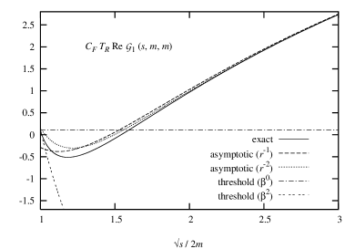
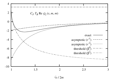
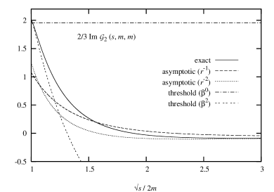
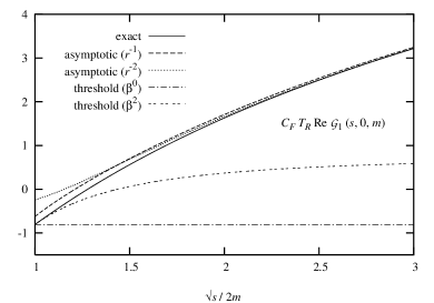
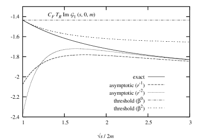
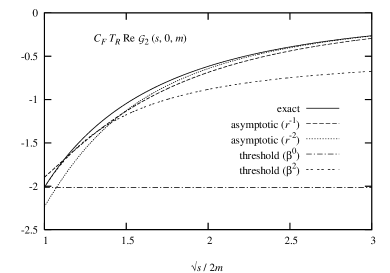
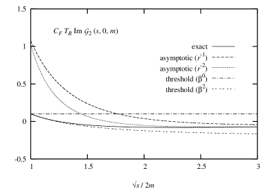
Figure 3: The real and imaginary parts of $C_{F}T_{R}{\cal G}_{1,2}(s,m,m)$ as functions of the rescaled c.m. energy and their threshold and asymptotic expansions.

Figure 4: The real and imaginary parts of $C_{F}T_{R}{\cal G}_{1,2}(s,0,m)$ as functions of the rescaled c.m. energy and their threshold and asymptotic expansions.

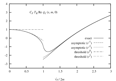
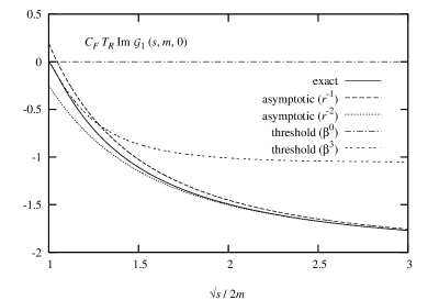
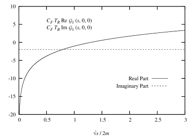
Figure 5: The real and imaginary parts of $C_{F}T_{R}{\cal G}_{1}(s,m,0)$ as functions of the rescaled c.m. energy and their threshold and asymptotic expansions.

Figure 6: The real and imaginary parts of $C_{F}T_{R}{\cal G}_{1}(s,0,0)$ as functions of the rescaled c.m. energy.

5 Summary

In this paper we calculated the triangle diagram contributions to the form factors of a heavy-quark axial vector current, of the flavor-singlet and non-singlet axial vector currents, and of the corresponding pseudoscalar currents to second order in the QCD coupling, for four different combinations of internal and external masses. Moreover, we have given the threshold and asymptotic expansions of these form factors to a degree of approximation which should prove useful for applications. We compared our exact results with these expansions at threshold and for large energies. For the threshold expansions we found that they approximate the exact results only over a very restricted energy range above threshold, and that at least the second order terms in the expansion are required for a reliable description. The large energy expansions appear to converge very well, and do in general yield a good description even for energies well below the asymptotic regime.

In this calculation we have used the implementation of the $\gamma_{5}$ matrix according to [7, 8] in dimensional regularization. This method is algebraically consistent and convenient for computations, but breaks chiral invariance in $D\neq 4.$ To restore chiral invariance in this scheme, finite counterterms are required. With the exception of the counterterm for the pseudoscalar singlet current, these were determined in [8] for massless quarks. In this work, we calculated all finite counterterms required by chiral invariance in this scheme for the case for massive quarks, including the counterterm for the pseudoscalar singlet current (which turns out to be zero). All counterterms agree with the massless results of [8], illustrating their purely ultraviolet origin. Using these counterterms, we have shown that the appropriately renormalized vertex functions satisfy the correct chiral Ward identities. This exemplifies for a non-trivial two-loop case that the counterterms of [8] can be applied, as expected, also to infrared-finite Green functions involving massive quarks. However, it is a separate issue to apply the method of [8] to Green functions (with massless and/or massive quarks) that are infrared-divergent – using dimensional regularization as well – and ask whether these Green functions satisfy the correct chiral Ward identities. We shall report on this issue and on applications of our results in this paper and in [1, 2] to the electroproduction and, in particular, to the forward-backward asymmetry of heavy quarks in a future publication.

References

• [1] W. Bernreuther, R. Bonciani, T. Gehrmann, R. Heinesch, T. Leineweber, P. Mastrolia and E. Remiddi, Nucl. Phys.   B706 (2005) 245 (hep-ph/0406046).
• [2] W. Bernreuther, R. Bonciani, T. Gehrmann, R. Heinesch, T. Leineweber, P. Mastrolia and E. Remiddi, Nucl. Phys.  B712 (2005) 229 (hep-ph/0412259).
• [3] [LEP Collaborations], “A combination of preliminary electroweak measurements and constraints on the standard model,” hep-ex/0412015.
• [4] J. A. Aguilar-Saavedra et al. [ECFA/DESY LC Physics Working Group Collaboration], “TESLA Technical Design Report Part III: Physics at an $e^{+}e^{-}$ Linear Collider”, DESY-report 2001-011 (hep-ph/0106315).
• [5] S. L. Adler, Phys. Rev.  177 (1969) 2426.
• [6] J. S. Bell and R. Jackiw, Nuovo Cim. A60 (1969) 47.
• [7] D. A. Akyeampong and R. Delbourgo, Nuovo Cim.  A17 (1973) 578.
• [8] S. A. Larin, Phys. Lett.   B303 (1993) 113 (hep-ph/9302240).
• [9] G. ’t Hooft and M. J. G. Veltman, Nucl. Phys.  B44 (1972) 189.
• [10] B. A. Kniehl and J. H. Kühn, Nucl. Phys. B329 (1990) 547.
• [11] R. Harlander and M. Steinhauser, Prog. Part. Nucl. Phys.  43 (1999) 167 (hep-ph/9812357).
• [12] V. A. Smirnov, Applied asymptotic expansions in momenta and masses, Springer Verlag (Heidelberg, 2002).
• [13] S. L. Adler and W. A. Bardeen, Phys. Rev.   182 (1969) 1517.
• [14] K.G. Chetyrkin, B.A. Kniehl, M. Steinhauser and W.A. Bardeen, Nucl. Phys. B535 (1998) 3 (hep-ph/9807241).
• [15] D. Espriu and R. Tarrach, Z. Phys.  C16 (1982) 77.
• [16] J.A.M. Vermaseren, Symbolic Manipulation with FORM, Version 2, CAN, Amsterdam, 1991; New features of FORM, (math-ph/0010025).
• [17] S. Laporta, Int. J. Mod. Phys. A15 (2000) 5087 (hep-ph/0102033).
• [18] T. Gehrmann and E. Remiddi, Nucl. Phys. B580 (2000) 485 (hep-ph/9912329).
• [19] A. V. Kotikov, Phys. Lett. B254 (1991) 158.
• [20] E. Remiddi, Nuovo Cim. A110 (1997) 1435 (hep-th/9711188).
• [21] M. Caffo, H. Czyż, S. Laporta and E. Remiddi, Acta Phys. Polon. B29 (1998) 2627 (hep-th/9807119).
M. Caffo, H. Czyż, S. Laporta and E. Remiddi, Nuovo Cim. A111 (1998) 365 (hep-th/9805118).
• [22] R. Bonciani, P. Mastrolia and E. Remiddi, Nucl. Phys. B661 (2003) 289 (hep-ph/0301170),[Erratum-ibid. Nucl. Phys. B702 (2004) 259].
• [23] R. Bonciani, P. Mastrolia and E. Remiddi, Nucl. Phys. B676 (2004) 399 (hep-ph/0307295).
• [24] R. Bonciani, P. Mastrolia and E. Remiddi, Nucl. Phys. B690 (2004) 138 (hep-ph/0311145).
• [25] E. Remiddi and J. A. M. Vermaseren, Int. J. Mod. Phys. A15 (2000) 725 (hep-ph/9905237).
• [26] T. Gehrmann and E. Remiddi, Comput. Phys. Commun. 141 (2001) 296 (hep-ph/0107173).
• [27] L. D. Landau, Dokl. Akad. Nauk, USSR 60 (1948) 207.
C.N. Yang, Phys. Rev. 77 (1950) 242.
• [28] R. Lewin, Polylogarithms and associated functions, North Holland (Amsterdam, 1984).