Polarization, CP Asymmetry and Branching ratios in $B\to K^{\ast}K^{\ast}$ with Perturbative QCD approach

Abstract

We study the charmless rare decays $B\to K^{\ast}K^{\ast}$ within the Perturbative QCD picture. We calculate not only factorizable and non-factorizable diagrams, but also annihilation ones. Our predictions are the following: The longitudinal polarization fraction vary from $75\%$ to $99\%$ depending on channels, the branching ratios are of order $10^{-7}$ for $B^{0}(\bar{B}^{0})\to K^{\ast 0}\bar{K}^{\ast 0}$ and $B^{\pm}\to K^{\ast\pm}\bar{K}^{\ast 0}(K^{\ast 0})$, much bigger than that for $B^{0}(\bar{B}^{0})\to K^{\ast+}K^{\ast-}$($10^{-8}$). The direct CP asymmetry in $B^{\pm}\to K^{\ast\pm}\bar{K}^{\ast 0}(K^{\ast 0})$ and $B^{0}(\bar{B}^{0})\to K^{\ast+}K^{\ast-}$ is about $-15\%$ and $-65\%$ if we choose $\alpha(\varphi_{2})$ as $95^{\circ}$. There’s no direct CPV in $B^{0}(\bar{B}^{0})\to K^{\ast 0}\bar{K}^{\ast 0}$ decays because of the pure $b\to d$ penguin topology. Our predictions will be tested in the future B experiments.

1 Introduction

Exclusive B meson decays, especially $B\to VV$ modes, have aroused more and more interest for both theorists and experimenters. Since it offers an attractive opportunity to get a deep insight into the flavor structure of the Standard Model (SM) and the CP violation parameters. But things are not so easy due to the Non-perturbative QCD dynamics. Several approaches, which include factorization approach (FA) [1, 2], QCD improved factorizations (QCDF ) [3, 4], Soft-collinear effective theory (SCET) [5] and Perturbative QCD (PQCD) [6, 7, 8] approach, have been developed to solve this problem. PQCD is based on $k_{T}$ factorization theorem [9, 10, 11] while others are most based on collinear factorization [12]. Besides, Sudakov factor and threshold resummation [9, 13] have been induced in PQCD to regulate the End-point singularities, so the arbitrary cutoffs [4] are no longer necessary.

In the PQCD framework the hard amplitudes for various topologies of diagrams, including factorizable, nonfactorizable and annihilation, are all six-quark amplitudes, while in FA and QCDF the leading factorizable diagrams involve four-quark amplitudes. This difference leads to a different characteristic scale, the former $\sqrt{\wedge m_{B}}\ \ (\sim 1.5GeV)$ [7, 8] and the latter $m_{B}$. Therefore, we get a larger Wilson coefficients ($C_{3-6}$) associated with the QCD penguin in PQCD due to the evaluation of the renormalization group, this means penguin diagrams have been enhanced dynamically. Current penguin dominated modes data, such as $B\to K\pi$ [14] and $B\to\phi K$ [15], seem to fit well with the PQCD predictions [7, 8, 16].

The recent $B\to\phi K^{*}$ data [17, 18] reveal a large transverse polarization fraction, which differs from most theoretical predictions and is considered as a puzzle. This indicates $B\to VV$ modes must be more complicated than we think and needs to be investigated more thoroughly. Motivated by this, we study another $B\to VV$ mode within the Standard Model (SM). $B\to K^{*}K^{*}$ decays, which governed by $B\to K^{*}$ form factors too, may help us to know more about the polarization puzzle, as well as the CKM phase angle $\alpha$ [19] and new physics. In the following sections, we will perform $B\to K^{\ast}K^{\ast}$ decays, which have the same topologies with $B\to KK$ [20], within the PQCD framework. Our goal is to find out the branching ratios, CP asymmetries, as well as the polarization fractions.

2 Framework and power counting

In the $B\to K^{\ast}K^{\ast}$ modes, the B meson is heavy and sitting at rest. It decays to two light vector mesons with large momenta. Therefore the $K^{\ast}$ mesons are moving very fast in the rest frame of B meson. In this case, the short distance hard process dominates the decay amplitude and Final State Interaction (FSI) may not be important in most of the cases, this makes the perturbative QCD applicable. For $B^{0}(\bar{B}^{0})\to K^{\ast+}K^{\ast-}$ decay, because of its small branching ratio, FSI may occur through intermediate states $\rho\rho$ or $K^{*0}\bar{K}^{*0}$, etc. If future experiments deviate theoretical prediction largely, it might be an indication of strong FSI effects. Here we give only the perturbative picture for experiments to test.

In PQCD approach, the decay amplitude is factorized into the convolution of the mesons’ light-cone wave functions, the hard scattering kernel and the Wilson coefficients, which stands for the soft, hard and harder dynamics respectively. The transverse momentum was introduced so that the endpoint singularity which will break the collinear factorization is regulated and the large double logarithm term appears after the integration on the transverse momentum, which is then resummed into the Sudukov form factor. The formalism can be written as:

$${\cal M}\sim \int dx_{1}dx_{2}dx_{3}b_{1}db_{1}b_{2}db_{2}b_{3}db_{3}Tr[C(t)\Phi_{B}(x_{1},b_{1})\Phi_{K^{*}}(x_{2},b_{2})\Phi_{K^{*}}(x_{3},b_{3})$$ (1)

$$H(x_{i},b_{i},t)S_{t}(x_{i})e^{-S(t)}],$$

where the $b_{i}$ is the conjugate space coordinate of the transverse momentum, which represents the transverse interval of the meson. $t$ is the largest energy scale in hard function $H$, while the jet function $S_{t}(x_{i})$ comes from the summation of the double logarithms $\ln^{2}x_{i}$, called threshold resummation [9, 13], which becomes large near the endpoint.

We use the effective Hamiltonian for the process $B\to K^{*}K^{*}$ given by [21]

$${\cal H}_{eff}=\frac{G_{F}}{\sqrt{2}}\left\{V_{u}\left[C_{1}(\mu)O_{1}(\mu)+C_{2}(\mu)O_{2}(\mu)\right]-V_{t}\sum_{i=3}^{10}C_{i}(\mu)O_{i}^{(q)}(\mu)\right\},$$ (2)

where the CKM matrix elements $V_{u}=V_{ud}^{*}V_{ub}$, $V_{t}=V_{td}^{*}V_{tb}$, $C_{i}(\mu)$ being the Wilson coefficients, and the operators

$$O_{1}=(\bar{d}_{i}u_{j})_{V-A}(\bar{u}_{j}b_{i})_{V-A},\,O_{2}=(\bar{d}_{i}u_{i})_{V-A}(\bar{u}_{j}b_{j})_{V-A},$$

$$O_{3}=(\bar{d}_{i}b_{i})_{V-A}\sum\limits_{q}(\bar{q}_{j}q_{j})_{V-A},\,O_{4}=(\bar{d}_{i}b_{j})_{V-A}\sum\limits_{q}(\bar{q}_{j}q_{i})_{V-A},$$

$$O_{5}=(\bar{d}_{i}b_{i})_{V-A}\sum\limits_{q}(\bar{q}_{j}q_{j})_{V+A},\,O_{6}=(\bar{d}_{i}b_{j})_{V-A}\sum\limits_{q}(\bar{q}_{j}q_{i})_{V-A},$$

$$O_{7}=\frac{3}{2}(\bar{d}_{i}b_{i})_{V-A}\sum\limits_{q}e_{q}(\bar{q}_{j}q_{j})_{V+A},\,O_{8}=\frac{3}{2}(\bar{d}_{i}b_{j})_{V-A}\sum\limits_{q}e_{q}(\bar{q}_{j}q_{i})_{V+A},$$

$$O_{9}=\frac{3}{2}(\bar{d}_{i}b_{i})_{V-A}\sum\limits_{q}e_{q}(\bar{q}_{j}q_{j})_{V-A},\,O_{10}=\frac{3}{2}(\bar{d}_{i}b_{j})_{V-A}\sum\limits_{q}e_{q}(\bar{q}_{j}q_{i})_{V-A}.$$ (3)

i and j stand for $SU(3)$ color indices.

Now let’s analyze these decay channels topologically. First, it is categorized emission and annihilation diagrams. Second, each category can be extracted to 4 diagrams, two factorizable and two nonfactorizable, in the leading order. Let’s take $Fig.1(a)$ for instance, the spectator quark can be attached to each of the quark coming from the 4-quark operators with a hard gluon.

For the $B^{0}(\bar{B}^{0})\to K^{\ast 0}\bar{K}^{\ast 0}$ decays ($Fig.1$), only the operators $O_{3-10}$ contribute via penguin topology with light quark $q=s$ ($diagram\ a$) and via annihilation topology with the light quark $q=d$ ($diagram\ b\ and\ c$) or $s$ ($diagram\ d$). It is a pure penguin mode with only one kind of CKM element, as a result, it will not generate any difference between $B^{0}$ and $\bar{B}^{0}$ decay and hence no direct CP violation. Using the PQCD power counting rules [7], We can first predict that the main contribution came from the factorizable parts of the emission diagram $F_{Le4}$(F stands for factorizable, L stands for longitudinal, e stands for emission and $4$ stands for the operator involved) with a large Wilson coefficient $C_{4}+C_{3}/3-C_{10}/2-C_{9}/6$. The operator $O_{6}$ disappear here because the vector meson $\bar{K}^{*0}$ can not be produced through a $(S-P)(S+P)$ operator. But in $B\to K^{0}\bar{K}^{0}$ decay [20], there isn’t such constraint and the predicted branching ratio is about three times bigger than ours. Second, the transverse parts of the emission diagram($F_{Ne4}$ and $F_{Te4}$) are down by a factor $r_{k^{*}}(r_{K^{*}}\simeq m_{K^{*}}/m_{B})$ or $r_{K^{*}}^{2}$, then the longitudinal parts($F_{Le4}$) dominate this process and give a large longitudinal polarization fraction. Third, nonfactorizable amplitudes $M$, including both emission and annihilation diagrams, are suppressed by a power of $\bar{\Lambda}/M_{B}$ when compared with factorizable ones. At last, we can forecast the factorizable parts of the annihilation diagrams ($c,d$) counteract separately in most of the cases, to be exactly, $F_{La3(5)}$ and $F_{Na(5)}$ vanish and $F_{Ta3(5)}$ survive but suppressed by $r_{k^{*}}^{2}$, this makes the emission diagram relatively more important. The factorizable parts for the space-like annihilation diagram ($b$) with operator $(S-P)(S+P)$ and Wilson coefficient $C_{6}+C_{5}/3-C_{8}/2-C_{7}/6$ do not counteract in any case but is still not big enough to play the most important role. It is about 10 times smaller than the emission ones after calculation.

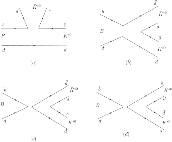
Figure 1: Diagrams for $B^{0}\rightarrow K^{*0}\bar{K}^{*0}$

Things are different for the $B^{\pm}\to K^{\ast\pm}\bar{K}^{\ast 0}(K^{\ast 0})$ decays($Fig.2$). The operators $O_{3-10}$ contribute via penguin topology with the light quark $q=s$ ($diagram\ a$) and via the annihilation topology with $q=u$ ($diagram\ b$), while tree operator $O_{1,2}$ also contribute via annihilation topology ($diagram\ c$). We can see that there are two kinds of CKM elements, $V_{u}$ from tree and $V_{t}$ from penguin, that will induce weak phase and CP violation. We can get diagram 2.(a) and 2.(b) by replacing the d quark in $Fig.1$ (a) and (b) to u quark. It makes no difference for power counting and the conclusion we have given doesn’t change. Diagram (c) is a tree diagram, we have a much bigger Wilson coefficient $C_{2}+C_{1}/3$ for the factorizable parts and $C_{1}$ for the nonfactorizable parts, but at the same time, it is an annihilation diagram, as we have stated, $F_{L}$ and $F_{N}$ vanish and $F_{T}$ is suppressed by $r_{K^{*}}^{2}$ in this kind of diagram. After taken account of all these two aspects, we can foresee that this diagram will be big but not big enough to increase the branching ratio largely, we also believe the transverse parts will play a more important role than that of the former channel. Our calculation is consistent with our predictions and will be shown in next section.

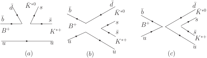
Figure 2: Diagrams for $B^{+}\rightarrow K^{*+}\bar{K}^{*0}$

We put the diagrams of $B^{0}(\bar{B}^{0})\to K^{\ast+}K^{\ast-}$ decays in Fig.3. From the topology we know that $O_{3-10}$ contribute via annihilation topology with the light quark $q=u$ ($diagram\ b$) or $s$ ($diagram\ c$) and tree operator $O_{1,2}$ contribute via annihilation topology ($diagram\ a$). CPV occurs in this channels for the same reason we have given for $B^{+}\to K^{*+}K^{*0}$. But when referring to the branching ratio, it is far different from the former two, cause it’s a pure annihilation mode and the emission diagram which gives the main contribution to the branching ratio of the former two channels no longer exist in this process, so we can expect a smaller branching ratio for this channel. Besides, the tree diagram involve $C_{1}+C_{2}/3$ for factorizable parts and $C_{2}$ for nonfactorizble parts. As is well-known, $C_{1}+C_{2}/3$ is small (about 0.1 when $t=4.8GeV$) but $C_{2}$ is as big as 1.1 ($t=4.8GeV$), so the factorizable parts can not be so important as the former two. Indeed, we found the nonfactorizable tree diagram is the biggest one though it is nonfactorizable suppressed after calculation. All our calculations fit well with the predictions and they are shown in section 3.

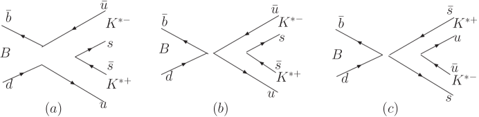
Figure 3: Diagrams for $B^{0}\rightarrow K^{*+}K^{*-}$

Now we are going to extract these decay channels within the PQCD framework. For convenience, We adopt the light-cone coordinate system [22], then the four-momentum of the B meson and the two $K^{*}$ mesons in the final state can be written as:

$$P_{1}=\frac{M_{B}}{\sqrt{2}}(1,1,{\bf 0_{T}}),$$

$$P_{2}=\frac{M_{B}}{\sqrt{2}}(1-r^{2}_{K^{*}},r^{2}_{K^{*}},{\bf 0_{T}}),$$

$$P_{3}=\frac{M_{B}}{\sqrt{2}}(r^{2}_{K^{*}},1-r^{2}_{K^{*}},{\bf 0_{T}}),$$ (4)

in which $r_{K^{*}}$ is defined by $r^{2}_{K^{*}}=\frac{1}{2}(1-\sqrt{1-4M_{K^{*}}^{2}/M_{B}^{2}})\simeq M_{K^{*}}^{2}/M_{B}^{2}\ll 1$. To extract the helicity amplitudes, we parameterize the polarization vectors. The longitudinal polarization vector must satisfy the orthogonality and normalization : ${\epsilon_{2L}\cdot P_{2}}=0,\,\,{\epsilon_{3L}\cdot P_{3}}=0$, and ${\epsilon_{2L}}^{2}={\epsilon_{3L}}^{2}=-1$. Then we can give the manifest form as follows:

$${\epsilon_{2L}}=\frac{1}{\sqrt{2}r_{K^{*}}}(1-r^{2}_{K^{*}},-r^{2}_{K^{*}},{\bf 0_{T}}),$$

$${\epsilon_{3L}}=\frac{1}{\sqrt{2}r_{K^{*}}}(-r^{2}_{K^{*}},1-r^{2}_{K^{*}},{\bf 0_{T}}).$$ (5)

As to the transverse polarization vectors, we can choose the simple form:

$${\epsilon_{2T}}=\frac{1}{\sqrt{2}}(0,0,{\bf 1_{T}}),$$

$${\epsilon_{3T}}=\frac{1}{\sqrt{2}}(0,0,{\bf 1_{T}}).$$ (6)

The decay width for these channels is :

$$\Gamma=\frac{G_{F}^{2}{\bf|P_{c}|}}{16\pi M_{B}^{2}}\sum\limits_{\sigma=L,T}{\cal M}^{\sigma{\dagger}}{\cal M}^{\sigma}$$ (7)

where ${\bf P_{c}}$ is the 3-momentum of the final state meson, and $|{\bf P_{c}}|=\frac{M_{B}}{2}(1-2r^{2}_{K^{*}})$. ${\cal M}^{\sigma}$ is the decay amplitude which is decided by QCD dynamics, will be calculated later in PQCD approach. The subscript $\sigma$ denotes the helicity states of the two vector mesons with L(T) standing for the longitudinal (transverse) components. After analyzing the Lorentz structure, the amplitude can be decomposed into:

$${\cal M}^{\sigma}=M_{B}^{2}{\cal M}_{L}+M_{B}^{2}{\cal M}_{N}\epsilon^{\ast}_{2}(\sigma=T)\cdot\epsilon^{\ast}_{3}(\sigma=T)+i{\cal M}_{T}\epsilon_{\mu\nu\rho\sigma}\epsilon_{2}^{\mu\ast}\epsilon_{3}^{\nu\ast}P_{2}^{\rho}P_{3}^{\sigma}.$$ (8)

We can define the longitudinal $H_{0}$, transverse $H_{\pm}$ helicity amplitudes

$$H_{0}=M^{2}_{B}{\cal M}_{L},\,\,H_{\pm}=M^{2}_{B}{\cal M}_{N}\mp M_{K^{*}}^{2}\sqrt{r^{\prime 2}-1}{\cal M}_{T},$$ (9)

where $r^{\prime}=\frac{P_{2}\cdot P_{3}}{M_{K^{*}}^{2}}$. After the helicity summation, we can deduce that they satisfy the relation

$$\sum\limits_{\sigma=L,R}{\cal M}^{\sigma{\dagger}}{\cal M}^{\sigma}=|H_{0}|^{2}+|H_{+}|^{2}+|H_{-}|^{2}.$$ (10)

There is another equivalent set of definition of helicity amplitudes

$$A_{0}=-\xi M^{2}_{B}{\cal M}_{L},$$

$$A_{\|}=\xi\sqrt{2}M^{2}_{B}{\cal M}_{N},$$

$$A_{\perp}=\xi M_{K^{*}}^{2}\sqrt{r^{\prime 2}-1}{\cal M}_{T},$$ (11)

with $\xi$ the normalization factor to satisfy

$$|A_{0}|^{2}+|A_{\|}|^{2}+|A_{\perp}|^{2}=1,$$ (12)

where the notations $A_{0}$, $A_{\|}$, $A_{\perp}$ denote the longitudinal, parallel, and perpendicular polarization amplitude.

What is followed is to calculate the matrix elements ${\cal M}_{L}$, ${\cal M}_{N}$ and ${\cal M}_{T}$ of the operators in the weak Hamiltonian with PQCD approach. We have to admit the light cone wave functions of mesons are not calculable in principal in PQCD, but they are universal for all the decay channels. So that they can be constraint from the measured other decay channels, like $B\rightarrow K\pi$ and $B\rightarrow\pi\pi$ decays etc [7, 8]. For the heavy B meson, we have

$$\frac{1}{\sqrt{2N_{c}}}(\not\!P_{1}+M_{B})\gamma_{5}\phi_{B}(x,b).$$ (13)

For longitudinal polarized $K^{*}$ meson,

$$\frac{1}{\sqrt{2N_{c}}}[M_{K^{*}}\not\!\epsilon_{2L}\phi_{K^{*}}(x)+\not\!\epsilon_{2L}\not\!P_{2}\phi_{K^{*}}^{t}(x)+M_{\phi}I\phi^{s}_{K^{*}}(x)],$$ (14)

and for transverse polarized $K^{*}$ meson,

$$\frac{1}{\sqrt{2N_{c}}}[M_{K^{*}}\not\!\epsilon_{2T}\phi^{v}_{K^{*}}(x)+\not\!\epsilon_{2T}\not\!P_{2}\phi_{K^{*}}^{T}(x)+\frac{M_{K^{*}}}{P_{2}\cdot n_{-}}i\epsilon_{\mu\nu\rho\sigma}\gamma_{5}\gamma^{\mu}\epsilon_{2T}^{\nu}P_{2}^{\rho}n_{-}^{\sigma}\phi^{a}_{K^{*}}(x)].$$ (15)

In the following concepts, we omit the subscript of the $K^{*}$ meson for simplicity.

The hard amplitudes are channel dependent, but they are perturbative calculable. The amplitudes for $B^{0}\to K^{\ast 0}\bar{K}^{\ast 0}$ and $\bar{B}^{0}\to K^{\ast 0}\bar{K}^{\ast 0}$are written as

$${\cal M}_{H} = f_{K^{*}}V_{t}^{*}F_{He4}+f_{B}V_{t}^{*}\left(\sum_{i=3}^{6}F_{Hai}^{(d)}+\sum_{i=3,5}F_{Hai}^{(s)}\right)$$ (16)

$$+V_{t}^{*}\left(\sum_{i=3,5}{\cal M}_{Hei}+\sum_{i=3}^{6}{\cal M}_{Hai}^{(d)}+\sum_{i=4,6}{\cal M}_{Hai}^{(s)}\right),$$

$$\bar{\cal M}_{H} = f_{K^{*}}V_{t}F_{He4}+f_{B}V_{t}\left(\sum_{i=3}^{6}F_{Hai}^{(d)}+\sum_{i=3,5}F_{Hai}^{(s)}\right)$$ (17)

$$+V_{t}\left(\sum_{i=3,5}{\cal M}_{Hei}+\sum_{i=3}^{6}{\cal M}_{Hai}^{(d)}+\sum_{i=4,6}{\cal M}_{Hai}^{(s)}\right).$$

respectively, where the subscript $H=L,N,T$ denotes different helicity amplitudes, and e(a) denotes the emission(annihilation) topology. The hard parts for the factorizable amplitudes $F$ and for the nonfactorizable amplitudes $\cal M$ are derived by contracting the wave function to the lowest-order one-gluon-exchange diagrams.

The helicity amplitudes ${\cal M}^{+}$ and ${\cal M}^{-}$ corresponding to $B^{+}\to K^{*+}\bar{K}^{*0}$ and $B^{-}\to K^{*-}K^{*0}$ are written as

$${\cal M}_{H}^{+} = V_{u}^{*}T_{H}-V_{t}^{*}P_{H}$$ (18)

$${\cal M}_{H}^{-} = V_{u}T_{H}-V_{t}P_{H}$$ (19)

with

$$T_{H}=f_{B}F_{Ha2}^{(u)}+{\cal M}_{Ha1}^{(u)}$$

and

$$P_{H}=f_{K^{*}}F_{He4}+f_{B}\sum_{i=4,6}F_{Hai}^{(d)}+\sum_{i=3,5}{\cal M}_{Hei}+\sum_{i=3,5}{\cal M}_{Hai}^{(d)}.$$

The helicity amplitudes for $B^{0}\to K^{*+}K^{*-}$ and $\bar{B}^{0}\to K^{*+}K^{*-}$ are written as

$${\cal M}_{H}^{\prime} = V_{u}^{*}T_{H}^{\prime}-V_{t}^{*}P_{H}^{\prime}$$ (20)

$$= V_{u}^{*}\left(f_{B}F_{Ha1}^{(u)}+{\cal M}_{Ha2}^{(u)}\right)-V_{t}^{*}\sum_{q=u,s}\left(f_{B}\sum_{i=3,5}F_{Hai}^{(q)}+\sum_{i=4,6}{\cal M}_{Hai}^{(q)}\right),$$

$$\bar{\cal M}_{H}^{\prime} = V_{u}T_{H}^{\prime}-V_{t}P_{H}^{\prime}$$ (21)

$$= V_{u}\left(f_{B}F_{Ha1}^{(u)}+{\cal M}_{Ha2}^{(u)}\right)-V_{t}\sum_{q=u,s}\left(f_{B}\sum_{i=3,5}F_{Hai}^{(q)}+\sum_{i=4,6}{\cal M}_{Hai}^{(q)}\right),$$

where the $F_{Lai}^{(q)}$ and $F_{Nai}^{(q)}$ vanish and $F_{Tai}^{(q)}$ takes from of Eqs.(58,59). The detailed formulas with polarization ${\cal M}_{L}$, ${\cal M}_{N}$, and ${\cal M}_{T}$ for each diagram are given in the appendix.

3 Numerical analysis

For the B meson wave function used in eq.(13), we employ the model [7, 8, 23]

$$\phi_{B}(x)=N_{B}x^{2}(1-x)^{2}\exp\left[-\frac{1}{2}(\frac{xM_{B}}{\omega_{B}})^{2}-\frac{\omega^{2}_{B}b^{2}}{2}\right],$$ (22)

where the shape parameter $\omega_{B}=0.4GeV$ has been constrained in other decay modes. The normalization constant $N_{B}=91.784GeV$ is related to the B decay constant $f_{B}=0.19GeV$. It is one of the two leading twist B meson wave functions; the other one is power suppressed, so we omit its contribution in the leading power analysis [24]. The $K^{*}$ meson distribution amplitude up to twist-3 are given by [30] with QCD sum rules.

$$\phi_{K^{*}}(x)=\frac{3f_{K^{*}}}{\sqrt{2N_{c}}}x(1-x)[1+0.57(1-2x)+0.07C_{2}^{3/2}(1-2x)],$$ (23)

$$\phi^{t}_{K^{*}}(x)=\frac{f_{K^{*}}^{T}}{2\sqrt{2N_{c}}}\left\{0.3(1-2x)[3(1-2x)^{2}+10(1-2x)-1]+1.68C_{4}^{1/2}(1-2x)\right.$$

$$\left.\ \ \ \ \ \ \ \ \ \ \ \ +0.06(1-2x)^{2}[5(1-2x)^{2}-3]+0.36\left\{1-2(1-2x)[1+\ln(1-x)]\right\}\right\},$$ (24)

$$\phi^{s}_{K^{*}}(x)=\frac{f_{K^{*}}^{T}}{2\sqrt{2N_{c}}}\left\{3(1-2x)\left[1+0.2(1-2x)+0.6(10x^{2}-10x+1)\right]\right.$$

$$\left.\ \ \ \ \ \ \ \ \ \ \ \ -0.12x(1-x)+0.36[1-6x-2\ln{(1-x)}]\right\}.$$ (25)

$$\phi^{T}_{K^{*}}(x)=\frac{3f_{K^{*}}^{T}}{\sqrt{2N_{c}}}x(1-x)[1+0.6(1-2x)+0.04C_{2}^{3/2}(1-2x)],$$ (26)

$$\phi^{v}_{K^{*}}(x)=\frac{f_{K^{*}}^{T}}{2\sqrt{2N_{c}}}\left\{\frac{3}{4}[1+(1-2x)^{2}+0.44(1-2x)^{3}]\right.$$

$$\left.\ \ \ \ \ \ \ \ \ \ \ \ +0.4C_{2}^{1/2}(1-2x)+0.88C_{4}^{1/2}(1-2x)+0.48[2x+\ln(1-x)]\right\},$$ (27)

$$\phi^{a}_{K^{*}}(x)=\frac{f_{K^{*}}^{T}}{4\sqrt{2N_{c}}}\left\{3(1-2x)[1+0.19(1-2x)+0.81(10x^{2}-10x+1)]\right.$$

$$\left.\ \ \ \ \ \ \ \ \ \ \ \ -1.14x(1-x)+0.48[1-6x-2\ln(1-x)]\right\},$$ (28)

where the Gegenbauer polynomials are

$$C_{2}^{\frac{1}{2}}(\xi)=\frac{1}{2}(3\xi^{2}-1),$$ (29)

$$C_{4}^{\frac{1}{2}}(\xi)=\frac{1}{8}(35\xi^{4}-30\xi^{2}+3),$$ (30)

$$C_{2}^{\frac{3}{2}}(\xi)=\frac{3}{2}(5\xi^{2}-1).$$ (31)

In paper [25], Li has suggested to reanalyze the $K^{*}$ meson distribution amplitude in order to solve the polarization puzzle of $B\to\phi K^{*}$. In that channel, Babar [18] and Belle [17] have reported a longitudinal polarization fraction($R_{L}$) small to $50\%$, it is different from most theoretical predictions and is considered as a puzzle. Many discussions have been given [26, 27, 28, 29] and among which Hsiang-nan Li argued a smaller $B\to K^{*}$ form factor($A_{0}\approx 0.3$), which doesn’t contradict any existing data, and hence a new distribution amplitude for $K^{*}$ meson. Any how, this assumption need to be justified by experiment and we will take the traditional wave function in this letter. If future experiment confirms a smaller $B\to K^{*}$ form factor and those argues, we just replace the wave function and get a smaller $R_{L}$ (about $65\%$) and smaller branching ratios (about $3\times 10^{-7}$) immediately. On the other hand, if future experiments find a small $R_{L}$ and branching ratios for $B^{0}(B^{+})\to K^{*0}(K^{*+})\bar{K}^{*0}$, it may be a support for a smaller $B\to K^{*}$ form factor and the validity of PQCD.

We employ the constants as follows [14]: the Fermi coupling constant $G_{F}=1.16639\times 10^{-5}GeV^{-2}$, the meson masses $M_{B}=5.28GeV,\ M_{K^{*}}=0.89GeV$, the decay constants $f_{K^{*}}=0.217GeV,\ f_{K^{*}}^{T}=0.16GeV$ [32], the central value of the CKM matrix elements $|V_{td}|=0.0075,\ |V_{tb}|=0.9992,\ |V_{ud}|=0.9745,\ |V_{ub}|=0.0033$ and the B meson lifetime $\tau_{B^{0}}=1.536ps$$\ (\tau_{B^{\pm}}=1.671ps)$ [14].

If we choose the CKM phase angle $\alpha(\varphi_{2})=95^{\circ}$ [14], then our our numerical results are given in TABLE.1, where $\phi_{\parallel}\equiv Arg(A_{\parallel}/A_{0})$ and $\phi_{\perp}\equiv Arg(A_{\perp}/A_{0})$. From the table we are convinced more with our power counting stated in chapter 2. We also find the polarization fraction $R_{\|}\simeq R_{\perp}$ and relative phase is around 2.6 for the former 3 channels. This is good news both for us and PQCD, since the current $B\to\phi K^{*}$ data [17, 18], which is also governed by the $B\to K^{*}$ form factors, suggest $R_{\|}\simeq R_{\perp}$, $\phi_{\|}\simeq 2.3$ and $\phi_{\perp}\simeq 2.5$. These data are contrary from those rescattering effects [29] and seem to support the evaluation of the relative strong phase in PQCD.

TABLE.1.  Helicity amplitudes and relative phases

Channel BR$$(10^{-7})$$

3.5 0.78 0.12 0.10 2.8 2.8

4.0 0.75 0.10 0.15 2.6 2.4

5.5 0.88 0.08 0.04 2.7 3.0

0.22 0.99 0.005 0.005 4.1 2.2

1.1 0.99 0.005 0.003 3.6 1.9

To test the contribution from different parts separately, we take $B^{0}(\bar{B}^{0})\to K^{\ast 0}\bar{K}^{\ast 0}$ for example and classify the contributions into 4 kinds (see TABLE.2.): (1) full contribution, (2) without annihilation nor nonfactorizable contributions, (3) without annihilation contributions, (4) without nonfactorizable contributions. Form the table we are convinced the annihilation contribution play an important role to the branching ratio. The annihilation diagrams counteract with emission diagram severely, it even makes the branching ratio smaller when compared with the pure emission contribution. We also notice that contribution from the factorizable parts of the emission diagram is also bigger than the total branching ratio for $B(\bar{B})\to K^{\ast 0}\bar{K}^{\ast 0}$. As a result, if we change the form factor $A_{0}$ from 0.4 to 0.32 as [25], then our calculation give a branching ratio of $2.3\times 10^{-7}$.

TABLE.2.  Contribution from different parts:
(1) full contribution, (2) without annihilation
nor nonfactorizable contributions, (3) without
annihilation contributions, (4) without nonfa
-ctorizable contributions.
Class	BR$(10^{-7})$	$|A_{0}|^{2}$	$|A_{\|}|^{2}$	$|A_{\perp}|^{2}$	$\phi_{\|}(rad)$	$\phi_{\perp}(rad)$
(1)	3.5	0.78	0.12	0.10	2.8	2.8
(2)	4.4	0.94	0.03	0.03	$\pi$	$\pi$
(3)	3.8	0.86	0.07	0.07	3.3	3.3
(4)	4.1	0.87	0.07	0.07	2.5	2.6

For $B^{+}\to K^{*+}\bar{K}^{*0}$ and $B^{-}\to K^{*-}K^{*0}$, it is similar to do so, we find annihilation diagrams contribute $7\%$ and $31\%$ to the total branching ratio respectively. If we take a smaller form factor and immediately get these values shown in TABLE.3. We have to say these results are rather roughly because no precision wave function for $K^{*}$ have been given in that paper.

TABLE.3.  The impact of a smaller form
factor $A_{0}=0.32$ on different channels
Decay Channel	BR$(10^{-7})$	$\ |A_{0}|^{2}\$	$\ |A_{\|}|^{2}\$	$|A_{\perp}|^{2}$
$B^{0}(\bar{B}^{0})\to K^{\ast 0}\bar{K}^{\ast 0}$	2.3	0.67	0.18	0.15
$B^{\pm}\to K^{*\pm}\bar{K}^{*0}(K^{*0})$	3.3	0.75	0.13	0.12

To extract the CPV parameter of $B^{+}\to K^{*+}\bar{K}^{*0}$ and $B^{-}\to K^{*-}K^{*0}$, we can rewrite the helicity amplitude in (18,19) as a function of the CKM phase angle $\alpha$:

$${\cal M}_{H}^{+} = V_{u}^{*}T_{H}-V_{t}^{*}P_{H}$$ (32)

$$= V_{u}^{*}T_{H}(1+Z_{H}e^{i(\alpha+{\delta}_{H})})$$

$${\cal M}_{H}^{-} = V_{u}T_{H}-V_{t}P_{H}$$ (33)

$$= V_{u}T_{H}(1+Z_{H}e^{i(-\alpha+{\delta}_{H})})$$

where $Z_{H}=|V_{t}^{*}/V_{u}^{*}||P_{H}/T_{H}|$, and $\delta$ is the relative strong phase between tree($T$) and penguin($P$) diagrams. Here in PQCD approach, the strong phase comes from the nonfactorizable diagrams and annihilation diagrams. This can be seen from Eqs.(75,102,105), where the modified Bessel function has an imaginary part. This is different from FA [1] and Beneke-Buchalla-Neubert-Sachrajda(BBNS) [3] approaches. In that approaches, annihilation diagrams are not taken into account, strong phases mainly come from the so-called Bander-Silverman-Soni mechanism [33]. As shown in [7], these effects are in fact next-to-leading-order($\alpha_{s}$ suppressed) elements and can be neglect in PQCD approach. We give the averaged branching ratio of $B^{\pm}\to K^{*\pm}\bar{K}^{*0}(K^{*0})$ as a function of $\alpha$ in Fig.4.

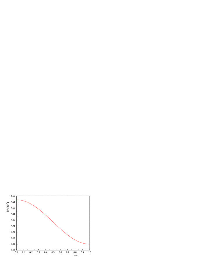
Figure 4: Average branching ratios of $B^{\pm}\rightarrow K^{*\pm}\bar{K}^{*0}(K^{*0})$ as a function of $\alpha$.

Using Eqs.(32,33), the direct CP violating parameter is

$$A^{dir}_{CP} = \frac{{|M^{+}|}^{2}-{|M^{-}|}^{2}}{{|M^{+}|}^{2}+{|M^{-}|}^{2}}$$ (34)

$$= \frac{-2sin\alpha\left(T_{L}^{2}sin\delta_{L}+2T_{N}^{2}sin\delta_{N}+2T_{T}^{2}sin\delta_{T}\right)}{T_{L}^{2}(1+Z_{L}^{2}+2Z_{L}cos\alpha cos\delta_{L})+2\sum_{i=N,T}T_{i}^{2}\left(1+Z_{i}^{2}+2Z_{i}cos\alpha cos\delta_{i}\right)}.$$

Since the transverse polarization is twice of freedom when comparing with longitudinal one, the factor before $T_{N}$ and $T_{T}$ is twice as $T_{L}$. If we choose $\alpha$ as $95^{\circ}$, then the direct CP asymmetry $A_{CP}^{dir}$ for these channels are:

$$A_{CP}^{dir}(B^{0}(\bar{B}^{0})\to K^{*0}\bar{K}^{*0}) = 0,$$ (35)

$$A_{CP}^{dir}(B^{\pm}\to K^{\ast\pm}\bar{K}^{\ast 0}(K^{\ast 0})) = -15\%,$$ (36)

$$A_{CP}^{dir}(B^{0}(\bar{B}^{0})\to K^{*+}K^{*-}) = -65\%.$$ (37)

We notice the CP asymmetry of $B^{0}(\bar{B}^{0})\to K^{*0}\bar{K}^{*0}$ is zero, since only pure penguin contribution in this channel. The CP asymmetry of $B^{\pm}\to K^{\ast\pm}\bar{K}^{\ast 0}(K^{\ast 0})$ is relatively small but large in $B^{0}(\bar{B}^{0})\to K^{*+}K^{*-}$, this is consistent with PQCD prediction. Using the power counting rules we stated in section.2, the former channel is penguin dominated while the latter one is tree dominated, then from the definition of $Z_{H}$ we can easily deduce a big $Z_{H}$ for the former channel and a small $Z_{H}$ for the latter one, so we can forecast a similar conclusion using Eqs.(34) without any calculation. We also notice the CP asymmetry for these channels are sensitive to $\alpha$, hence we put $A_{CP}^{dir}$ as a function of $\alpha$ in Fig.5.

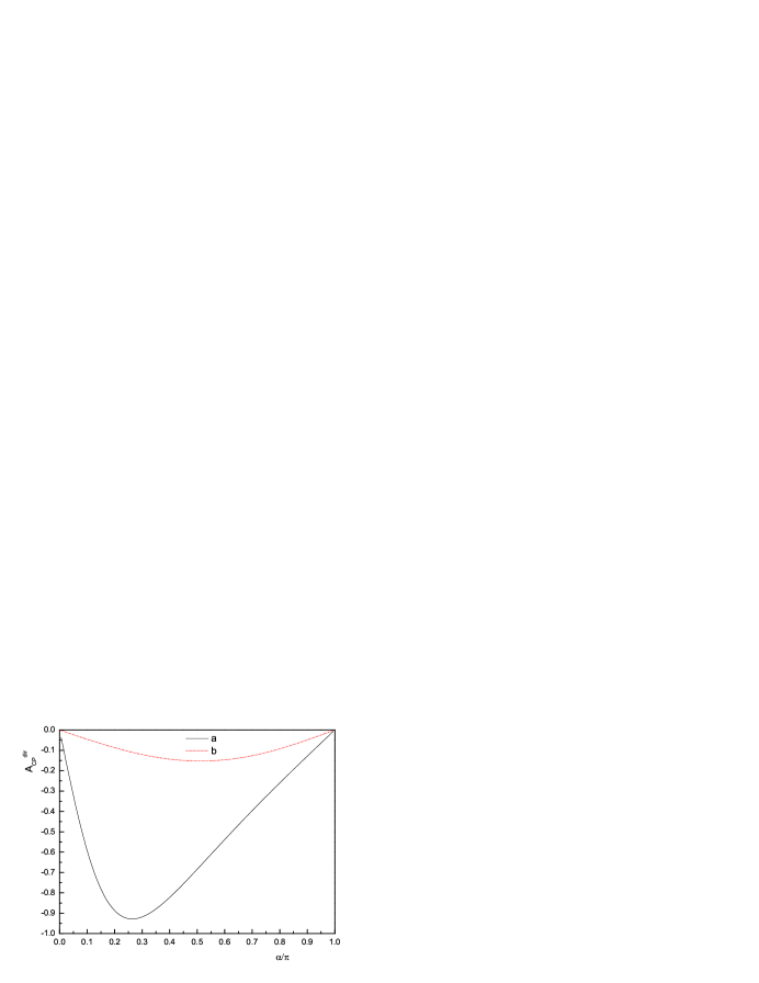
Figure 5: $A^{dir}_{CP}$ as a function of $\alpha$. (a) $B^{0}(\bar{B}^{0})\to K^{*+}K^{*-}$, (b) $B^{\pm}\to K^{*\pm}\bar{K}^{*0}$.

For the $B^{0}(\bar{B}^{0})\to K^{*+}K^{*-}$ decays, it is hard to distinguish $B^{0}$ and $\bar{B}^{0}$, we can use the value given in TABLE.1 to get an average branching ratio of $6.3\times 10^{-8}$. If we let CKM angle $\alpha$ as a free parameter, then the evaluation of averaged branching ratio is shown in Fig.6.

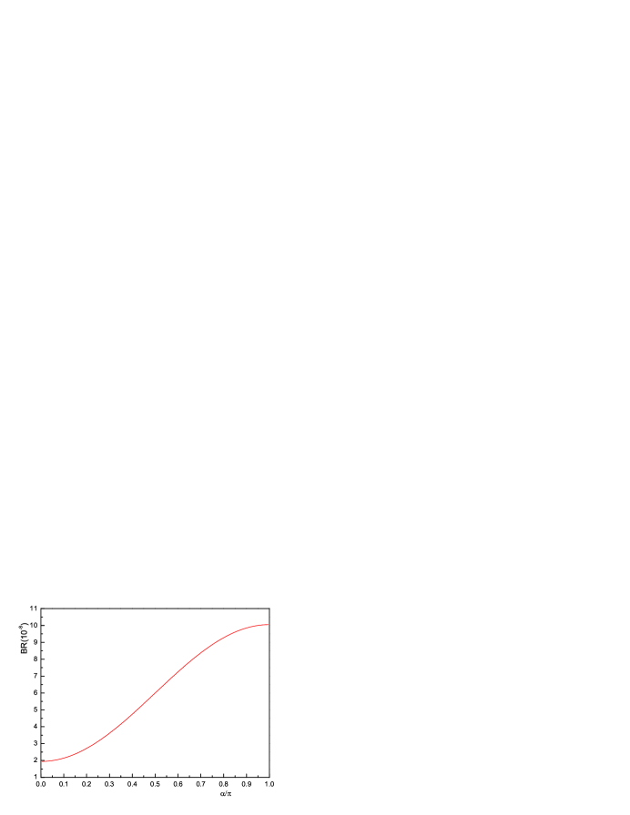
Figure 6: Average branching ratios of $B^{0}(\bar{B}^{0})\to K^{*+}K^{*-}$ as a function of $\alpha$.

When it refered to CP asymmetry of $B^{0}(\bar{B}^{0})$ decays, it is more complicated due to the $B^{0}-\bar{B}^{0}$ mixing. The CP asymmetry is time dependent:

$$A_{CP}(t)\simeq A^{dir}_{CP}cos(\Delta mt)+a_{\epsilon+\epsilon^{\prime}}sin(\Delta mt)$$ (38)

where $\Delta m$ is the mass difference of the two mass eigenstates of neutral $B$ mesons. The direct CP violation parameter $A^{dir}_{CP}$ is already defined in Eq.(34), while the mixing-related CP violation parameter is defined as

$$a_{\epsilon+\epsilon^{\prime}}=\frac{-2Im(\lambda_{CP})}{1+|\lambda_{CP}|^{2}},$$ (39)

where

$$\lambda_{CP}=\frac{V_{t}^{*}<f|H_{eff}|\bar{B}|>}{V_{t}<f|H_{eff}|B>}.$$ (40)

In these two channels, over $90\%$ of the branching ratios are composed of longitudinal fraction, so we can neglect the transverse contribution and use Eqs(20,21) to derive

$$\lambda_{CP}\simeq e^{2i\alpha}\frac{1+Z_{L}e^{i(\delta_{L}-\alpha)}}{1+Z_{L}e^{i(\delta_{L}+\alpha)}}.$$ (41)

People usually believe the penguin diagram contribution have been suppressed when comparing with the tree contribution. i.e. in $B(\bar{B})\to\pi^{+}\pi^{-}$ decay, Wilson coefficients of penguin diagram are loop suppressed, people believe $Z\ll 1$, $\lambda_{CP}\simeq exp[2i\alpha]$, $a_{\epsilon+\epsilon^{\prime}}=-sin2\alpha$, and $A^{dir}_{CP}\simeq 0$, then it is easy to extract $sin2\alpha$ through the measurement of CPV. However, $Z$ is not very small and $a_{\epsilon+\epsilon^{\prime}}$ is not a simple function of $-sin2\alpha$ even in $B(\bar{B})\to\pi^{+}\pi^{-}$ [8], hence we couldn’t get an exact $\alpha$ and this is called penguin pollution. In our channel, it is similar. After taking into account of the Wilson coefficient and the penguin enhancement we have stated, we get a $Z_{L}$ as large as $0.80$ and $\delta_{L}=2.35$. We put $a_{\epsilon+\epsilon^{\prime}}$ as a function of $\alpha$ in Fig.7 and we can see there isn’t a simple relationship between $a_{\epsilon+\epsilon^{\prime}}$ and $-sin2\alpha$.

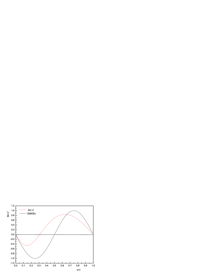
Figure 7: CP violation parameters $a_{\epsilon+\epsilon^{\prime}}$ of $B^{0}(\bar{B}^{0})\to K^{*+}K^{*-}$ as a function of $\alpha$

If we integrate the time variable t of Eq.(38), we will get the total CP asymmetry as

$$A_{CP}=\frac{1}{1+x^{2}}A_{CP}^{dir}+\frac{x}{1+x^{2}}a_{\epsilon+\epsilon^{\prime}}$$ (42)

with $x=\Delta m/\Gamma\simeq 0.771$ for the $B^{0}-\bar{B}^{0}$ mixing in SM [14]. The integrated CP asymmetries for $B^{0}(\bar{B}^{0})\to K^{*+}K^{*-}$ are shown in Fig.8. As for $B^{0}(\bar{B}^{0})\to K^{*0}\bar{K}^{*0}$, there is only penguin contribution in this decay, direct CP is zero in Eqs.(34). The weak phase of penguin $V_{tb}V_{td}^{*}$ is cancelled by the $B^{0}-\bar{B}^{0}$ mixing phase $V_{tb}^{*}V_{td}$, so $\lambda_{CP}$ (see Eqs.(40)) is real here and $a_{\epsilon+\epsilon^{\prime}}=0$. In fact, to the next leading order, there is a small up quark and charm quark penguin contribution which may give a small direct and mixing CP.

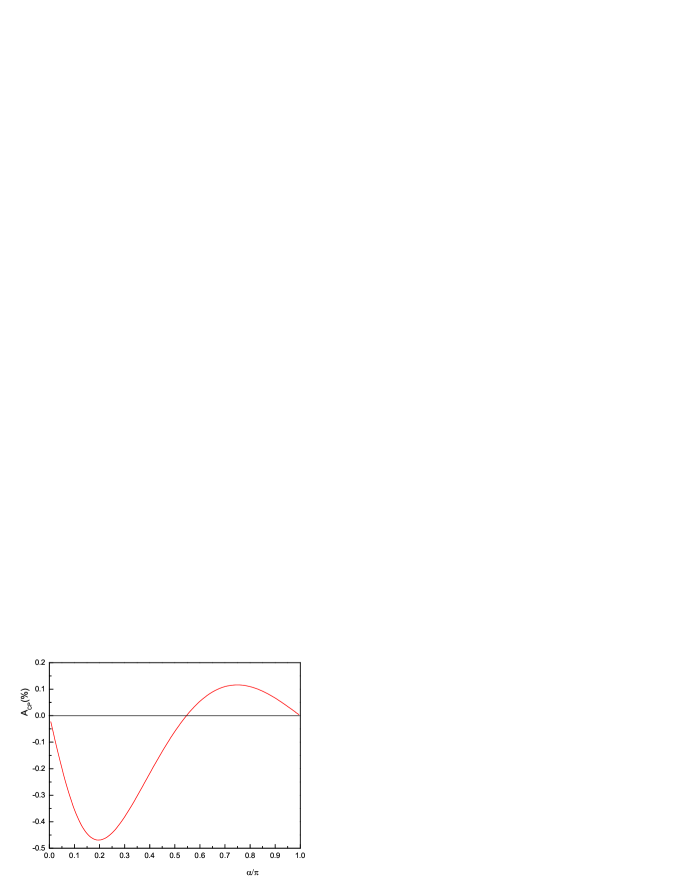
Figure 8: $A_{CP}$ of $B(\bar{B})\to K^{*+}K^{*-}$ as a function of $\alpha$

When the PQCD formalism is extended to $O(\alpha_{s}^{2})$, the hard scales can be determined more precisely and the scale independence of our predictions will be improved. Before this calculation is carried out, we consider the hard scales t located between $0.75-1.25$ times the invariant masses of the internal particles. For example, we take $t_{e}$(see Eqs.(77)) in the following range,

$${\rm max}(0.75\sqrt{x_{2}}M_{B},1/b_{1},1/b_{3}) <t_{e}^{(1)}< {\rm max}(1.25\sqrt{x_{2}}M_{B},1/b_{1},1/b_{3})\;,$$

$${\rm max}(0.75\sqrt{x_{1}}M_{B},1/b_{1},1/b_{3}) <t_{e}^{(2)}< {\rm max}(1.25\sqrt{x_{1}}M_{B},1/b_{1},1/b_{3}),$$ (43)

in order to estimate the $O(\alpha_{s}^{2})$ corrections. Then we can obtain the value area of the branching ratio for the penguin dominated modes

$$BR(B^{0}(\bar{B}^{0})\to K^{\ast 0}\bar{K}^{\ast 0})=(3.5^{+1.3}_{-0.7})\times 10^{-7},$$ (44)

$$BR(B^{\pm}\to K^{*\pm}\bar{K}^{*0}(K^{*0}))=(4.8^{+1.2}_{-0.8})\times 10^{-7},$$ (45)

which is sensitive to the change of $t$, so we can estimate that the next to leading order corrections will give about $20\%$ contribution. The ratios $R_{0},\,\,R_{\|}\,\,$and $R_{\perp}$ are not very sensitive to the variation of $t$, since the main contribution $F_{Le4}$, $F_{Ne4}$ and $F_{Te4}$ vary similarly when we conduct such changes on the maximum energy scale $t$. For the tree dominated modes $B^{0}(\bar{B}^{0})\to K^{*+}K^{*-}$, the evaluation of the Wilson coefficients $C_{1}$ and $C_{2}$ is slow, hence it is not sensitive to the scale $t$, we changed the parameter $\omega_{b}$ of the B meson wave function from 0.32 to 0.48 and found the absolute value for each integration become larger when $\omega_{b}=0.32$ and smaller when $\omega_{b}=0.48$, then the value area for these decays are

$$BR(B^{0}(\bar{B}^{0})\to K^{\ast+}{K}^{\ast-})=(6.4^{+0.5}_{-1.0})\times 10^{-8}.$$ (46)

If we compare our predictions with generalized FA [2]

$$BR(B^{0}(\bar{B}^{0})\to K^{\ast 0}\bar{K}^{\ast 0})=3.5\times 10^{-7},$$ (47)

$$BR(B^{\pm}\to K^{*\pm}\bar{K}^{*0}(K^{*0}))=3.7\times 10^{-7},$$ (48)

with $N_{c}=3$ and QCDF [34]

$$BR(B^{0}\to K^{\ast 0}\bar{K}^{\ast 0})=3.2\times 10^{-7},$$ (49)

$$BR(B^{-}\to K^{*-}K^{*0})=3.4\times 10^{-7},$$ (50)

with the form factor from Light cone sum rules(LCSR) [22, 35], we can easily find out their predictions for $B^{\pm}\to K^{*\pm}\bar{K}^{*0}(K^{*0})$ are a little smaller than our’s, and neither of them gives the branching ratios and CPV parameters of $B^{0}(\bar{B}^{0})\to K^{*+}\bar{K}^{*-}$, because annihilation diagrams can not be calculated in FA or QCDF in principle, while in PQCD all diagrams are calculated strictly. If we drop the annihilation contributions, we can get a similar results ($3.7\times 10^{-7}$) with them and they are already shown in TABLE.2. Current experiments [14] only give the upper limit for these decays

$$BR(B^{0}\to K^{\ast 0}\bar{K}^{\ast 0})<2.2\times 10^{-5},$$ (51)

$$BR(B^{+}\to K^{*+}K^{*0})<7.1\times 10^{-5},$$ (52)

$$BR(B\to K^{\ast+}\bar{K}^{\ast-})<1.41\times 10^{-4},$$ (53)

and future experiments are expected.

4 Summary

In this paper we have predicted the branching ratios, polarization fraction and CP asymmetries of $B\to K^{*}K^{*}$ modes using PQCD theorem in SM. We perform all leading diagrams, including both emission and annihilation diagrams, with up to twist-3 wave functions. The predicted branching ratios are compared with experiments and values from other approaches. We analyze the contribution from each parts for each decay channel, and found the annihilation diagrams is not very small to be neglected, then we present the dependence of the CP asymmetry and branching ratios on the CKM angle $\alpha$. We also discussed the potential impact of a smaller form factor $A_{0}$ in our paper.

Appendix A Factorization formulas

The factorizable amplitudes are written as

$$F_{Le4} = 8\pi C_{F}M_{B}^{2}\int_{0}^{1}dx_{1}dx_{2}\int_{0}^{\infty}b_{1}db_{1}b_{2}db_{2}\Phi_{B}(x_{1},b_{1})\ \left\{\left[(1+x_{2})\Phi_{K^{*}}(x_{2})\right.\right.$$ (54)

$$+\left.r_{K^{*}}(1-2x_{2})(\Phi^{t}_{K^{*}}(x_{3})+\Phi^{s}_{K^{*}}(x_{2}))\right]E_{e4}(t^{(1)}_{e})h_{e}(x_{1},x_{2},b_{1},b_{2})$$

$$\left.+\left[2r_{K^{*}}\Phi^{s}_{K^{*}}(x_{2})+r_{K^{*}}^{2}\phi_{K^{*}}(x_{2})\right]E_{e4}(t^{(2)}_{e})h_{e}(x_{2},x_{1},b_{2},b_{1})\right\}\;,$$

$$F_{Ne4} = 8\pi C_{F}M_{B}^{2}\int_{0}^{1}dx_{1}dx_{2}\int_{0}^{\infty}b_{1}db_{1}b_{2}db_{2}\Phi_{B}(x_{1},b_{1})$$ (55)

$$\times r_{K^{*}}\left\{[\Phi^{T}_{K^{*}}(x_{2})+2r_{K^{*}}\Phi^{v}_{K^{*}}(x_{2})+r_{K^{*}}x_{2}(\Phi^{v}_{K^{*}}(x_{2})-\Phi^{a}_{K^{*}}(x_{2}))]\right.$$

$$\times E_{e4}(t^{(1)}_{e})h_{e}(x_{1},x_{2},b_{1},b_{2})$$

$$\left.+r_{K^{*}}[\Phi^{v}_{K^{*}}(x_{2})+\Phi^{a}_{K^{*}}(x_{2})]E_{e4}(t^{(2)}_{e})h_{e}(x_{2},x_{1},b_{2},b_{1})\right\}\;,$$

$$F_{Te4} = 16\pi C_{F}M_{B}^{2}\int_{0}^{1}dx_{1}dx_{2}\int_{0}^{\infty}b_{1}db_{1}b_{2}db_{2}\Phi_{B}(x_{1},b_{1})$$ (56)

$$\times r_{K^{*}}\left\{[\Phi^{T}_{K^{*}}(x_{2})+2r_{K^{*}}\Phi^{a}_{K^{*}}(x_{2})+r_{K^{*}}x_{2}(\Phi^{a}_{K^{*}}(x_{2})-\Phi^{v}_{K^{*}}(x_{2}))]\right.$$

$$\times E_{e4}(t^{(1)}_{e})h_{e}(x_{1},x_{2},b_{1},b_{2})$$

$$\left.+r_{K^{*}}[\Phi^{v}_{K^{*}}(x_{2})+\Phi^{a}_{K^{*}}(x_{2})]E_{e4}(t^{(2)}_{e})h_{e}(x_{2},x_{1},b_{2},b_{1})\right\}\;,$$

$$F_{Ta1(2)}^{\left(u\right)} = 32\pi C_{F}M_{B}^{2}r_{k^{*}}^{2}\int_{0}^{1}dx_{2}dx_{3}\int_{0}^{\infty}b_{2}db_{2}b_{3}db_{3}$$ (57)

$$\times\left[(2-x_{2})(\Phi^{v}_{k^{*}}(x_{2})\Phi^{a}_{k^{*}}(x_{3})-\Phi^{a}_{k^{*}}(x_{2})\Phi^{v}_{k^{*}}(x_{3}))\right.$$

$$\left.+x_{2}(\Phi^{a}_{k^{*}}(x_{2})\Phi^{a}_{k^{*}}(x_{3})-\Phi^{v}_{k^{*}}(x_{2})\Phi^{v}_{k^{*}}(x_{3}))\right]$$

$$\times E_{a1(2)}^{(u)}(t_{au}^{(1)})h_{a}(1-x_{2},1-x_{3},b_{2},b_{3}),$$

$$F_{Ta3(4)}^{\left(d\right)} = 32\pi C_{F}M_{B}^{2}r_{k^{*}}^{2}\int_{0}^{1}dx_{2}dx_{3}\int_{0}^{\infty}b_{2}db_{2}b_{3}db_{3}$$ (58)

$$\times\left[(2-x_{2})(\Phi^{v}_{k^{*}}(x_{2})\Phi^{a}_{k^{*}}(x_{3})-\Phi^{a}_{k^{*}}(x_{2})\Phi^{v}_{k^{*}}(x_{3}))\right.$$

$$\left.+x_{2}(\Phi^{a}_{k^{*}}(x_{2})\Phi^{a}_{k^{*}}(x_{3})-\Phi^{v}_{k^{*}}(x_{2})\Phi^{v}_{k^{*}}(x_{3}))\right]$$

$$\times E_{a3(4)}^{(d)}(t_{ad}^{(1)})h_{a}(1-x_{2},1-x_{3},b_{2},b_{3}),$$

$$F_{Ta5}^{(d)} = -32\pi C_{F}M_{B}^{2}r_{k^{*}}^{2}\int_{0}^{1}dx_{2}dx_{3}\int_{0}^{\infty}b_{2}db_{2}b_{3}db_{3}$$ (59)

$$\times\left[(2-x_{2})(\Phi^{v}_{k^{*}}(x_{2})\Phi^{a}_{k^{*}}(x_{3})-\Phi^{a}_{k^{*}}(x_{2})\Phi^{v}_{k^{*}}(x_{3}))\right.$$

$$\left.+x_{2}(\Phi^{a}_{k^{*}}(x_{2})\Phi^{a}_{k^{*}}(x_{3})-\Phi^{v}_{k^{*}}(x_{2})\Phi^{v}_{k^{*}}(x_{3}))\right]$$

$$\times E_{a5}^{(d)}(t_{ad}^{(1)})h_{a}(1-x_{2},1-x_{3},b_{2},b_{3}),$$

$$F_{La6}^{\left(d\right)} = 32\pi C_{F}M_{B}^{2}r_{k^{*}}\int_{0}^{1}dx_{2}dx_{3}\int_{0}^{\infty}b_{2}db_{2}b_{3}db_{3}$$ (60)

$$\times\left[(1-x_{2})(\Phi^{s}_{k^{*}}(x_{2})+\Phi^{t}_{k^{*}}(x_{2}))\Phi_{k^{*}}(x_{3})+2\Phi_{k^{*}}(x_{2})\Phi^{s}_{k^{*}}(x_{3})\right]$$

$$\times E_{a6}^{(d)}(t^{(1)}_{ad})h_{a}(1-x_{2},1-x_{3},b_{2},b_{3}),$$

$$F_{Na6}^{\left(d\right)} = 32\pi C_{F}M_{B}^{2}r_{K^{*}}\int_{0}^{1}dx_{2}dx_{3}\int_{0}^{\infty}b_{2}db_{2}b_{3}db_{3}$$ (61)

$$\times(\Phi^{T}_{K^{*}}(x_{2})\left(\Phi^{v}_{K^{*}}(x_{3})-\Phi^{a}_{K^{*}}(x_{3})\right)E_{a6}^{(d)}(t^{(1)}_{ad})h_{a}(1-x_{2},1-x_{3},b_{2},b_{3}),$$

$$F_{Ta6}^{(d)} = 2F_{Na6}^{(q)},$$ (62)

$$F_{Ta3}^{\left(s\right)} = 32\pi C_{F}M_{B}^{2}r_{K^{*}}^{2}\int_{0}^{1}dx_{2}dx_{3}\int_{0}^{\infty}b_{2}db_{2}b_{3}db_{3}$$ (63)

$$\times\left[(1-x_{3})(\phi_{k^{*}}^{a}(x_{2})\phi_{k^{*}}^{a}(x_{3})-\phi_{k^{*}}^{v}(x_{2})\phi_{k^{*}}^{v}(x_{3}))\right.$$

$$\left.+(1+x_{3})(\phi_{k^{*}}^{v}(x_{2})\phi_{k^{*}}^{a}(x_{3})-\phi_{k^{*}}^{a}(x_{2})\phi_{k^{*}}^{v}(x_{3}))\right]$$

$$\times E_{a3}^{(s)}(t_{as}^{(1)})h_{a}(x_{3},x_{2},b_{3},b_{2}),$$

$$F_{Ta5}^{(s)} = -F_{Ta3}^{\left(s\right)}.$$ (64)

The last expression of the factorizable amplitudes $F_{Ta5}^{(s)}$ doesn’t really mean it equal to $F_{Ta3}^{(s)}$ but with the evolution factor $E_{Ta3}^{(s)}$ replaced by $E_{Ta5}^{(s)}$ and plus a factor $-1$ in the beginning. Other amplitudes which you can not find in the upper formulas must be equal to zero.

The factors $E(t)$ contain the evolution from the $W$ boson mass to the hard scales $t$ in the Wilson coefficients $a(t)$, and from $t$ to the factorization scale $1/b$ in the Sudakov factors $S(t)$:

$$E_{e4}^{(q)}\left(t\right) = \alpha_{s}\left(t\right)a_{4}^{(q)}(t)S_{B}\left(t\right)S_{K^{*}}\left(t\right)\;,$$

$$E_{ai}^{(q)}\left(t\right) = \alpha_{s}\left(t\right)a_{i}^{(q)}(t)S_{K^{*}}(t)S_{K^{*}}(t)\;.$$ (65)

The Wilson coefficients $a$ in the above formulas are given by

$$a_{1}^{(q)} = C_{1}+\frac{C_{2}}{N_{c}}\;,$$ (66)

$$a_{2}^{(q)} = C_{2}+\frac{C_{1}}{N_{c}}\;,$$ (67)

$$a_{3}^{(q)} = \left(C_{3}+\frac{C_{4}}{N_{c}}\right)+\frac{3}{2}e_{q}\left(C_{9}+\frac{C_{10}}{N_{c}}\right)\;,$$ (68)

$$a_{4}^{(q)} = \left(C_{4}+\frac{C_{3}}{N_{c}}\right)+\frac{3}{2}e_{q}\left(C_{10}+\frac{C_{9}}{N_{c}}\right)\;,$$ (69)

$$a_{5}^{(q)} = \left(C_{5}+\frac{C_{6}}{N_{c}}\right)+\frac{3}{2}e_{q}\left(C_{7}+\frac{C_{8}}{N_{c}}\right)\;,$$ (70)

$$a_{6}^{(q)} = \left(C_{6}+\frac{C_{5}}{N_{c}}\right)+\frac{3}{2}e_{q}\left(C_{8}+\frac{C_{7}}{N_{c}}\right).$$ (71)

$k_{T}$ resummation of large logarithmic corrections to the $B$, $K^{*}$ and $K^{*}$ meson distribution amplitudes lead to the exponentials $S_{B}$, $S_{K^{*}}$ and $S_{K^{*}}$, respectively.

$$S_{B}(t) = \exp\left[-s(x_{1}P_{1}^{+},b_{1})-2\int_{1/b_{1}}^{t}\frac{d{\bar{\mu}}}{\bar{\mu}}\gamma(\alpha_{s}({\bar{\mu}}^{2}))\right]\;,$$

$$S_{K^{*}}(t) = \exp\left[-s(x_{2}P_{2}^{+},b_{2})-s((1-x_{2})P_{2}^{+},b_{2})-2\int_{1/b_{2}}^{t}\frac{d{\bar{\mu}}}{\bar{\mu}}\gamma(\alpha_{s}({\bar{\mu}}^{2}))\right]\;,$$

$$S_{K^{*}}(t) = \exp\left[-s(x_{3}P_{3}^{-},b_{3})-s((1-x_{3})P_{3}^{-},b_{3})-2\int_{1/b_{3}}^{t}\frac{d{\bar{\mu}}}{\bar{\mu}}\gamma(\alpha_{s}({\bar{\mu}}^{2}))\right]\;,$$ (72)

The variables $b_{1}$, $b_{2}$, and $b_{3}$, conjugate to the parton transverse momenta $k_{1T}$, $k_{2T}$, and $k_{3T}$, represent the transverse extents of the $B$, $K^{*}$ and $K^{*}$ mesons, respectively. The quark anomalous dimension $\gamma=-{\alpha_{s}}/{\pi}$ and the so-called Sudakov factor $s(Q,b)$ is expressed as

$$s(Q,b) = \int_{1/b}^{Q}\!\!\frac{d\mu^{\prime}}{\mu^{\prime}}\left[\left\{\frac{2}{3}(2\gamma_{E}-1-\log 2)+C_{F}\log\frac{Q}{\mu^{\prime}}\right\}\frac{\alpha_{s}(\mu^{\prime})}{\pi}\right.$$ (73)

$$\left.+\left\{\frac{67}{9}-\frac{\pi^{2}}{3}-\frac{10}{27}n_{f}+\frac{2}{3}\beta_{0}\log\frac{\gamma_{E}}{2}\right\}\left(\frac{\alpha_{s}(\mu^{\prime})}{\pi}\right)^{2}\log\frac{Q}{\mu^{\prime}}\right].$$

The above Sudakov exponentials decrease fast in the large $b$ region, such that the $B\to K^{*}K^{*}$ hard amplitudes remain sufficiently perturbative in the end-point region.

The hard functions $h$’s are

$$h_{e}(x_{1},x_{2},b_{1},b_{2}) = K_{0}\left(\sqrt{x_{1}x_{2}}M_{B}b_{1}\right)S_{t}(x_{2})$$ (74)

$$\times\left[\theta(b_{1}-b_{2})K_{0}\left(\sqrt{x_{2}}M_{B}b_{1}\right)I_{0}\left(\sqrt{x_{2}}M_{B}b_{2}\right)\right.$$

$$\left.+\theta(b_{2}-b_{1})K_{0}\left(\sqrt{x_{2}}M_{B}b_{2}\right)I_{0}\left(\sqrt{x_{2}}M_{B}b_{1}\right)\right]\;,$$

$$h_{a}(x_{2},x_{3},b_{2},b_{3}) = \left(\frac{i\pi}{2}\right)^{2}H_{0}^{(1)}\left(\sqrt{x_{2}x_{3}}M_{B}b_{3}\right)S_{t}(x_{3})$$ (75)

$$\times\left[\theta(b_{2}-b_{3})H_{0}^{(1)}\left(\sqrt{x_{2}}M_{B}b_{2}\right)J_{0}\left(\sqrt{x_{2}}M_{B}b_{3}\right)\right.$$

$$\left.+\theta(b_{3}-b_{2})H_{0}^{(1)}\left(\sqrt{x_{2}}M_{B}b_{3}\right)J_{0}\left(\sqrt{x_{2}}M_{B}b_{2}\right)\right]\;.$$

We have proposed the parametrization for the evolution function $S_{t}(x)$ from threshold resummation[13].

$$S_{t}(x)=\frac{2^{1+2c}\Gamma(3/2+c)}{\sqrt{\pi}\Gamma(1+c)}[x(1-x)]^{c}\;.$$ (76)

where the parameter $c$ is chosen as $c=0.4$ for the $B\to K^{*}K^{*}$ decays. This factor modifies the end-point behavior of the meson distribution amplitudes, rendering them vanish faster at $x\to 0$. Threshold resummation for nonfactorizable diagrams is weaker and negligible. $K_{0},I_{0},H_{0}$ and $J_{0}$ are the Bessel functions.

The hard scales $t$ are chosen as the maxima of the virtualities of the internal particles involved in the hard amplitudes, including $1/b_{i}$:

$$t_{e}^{(1)} = {\rm max}(\sqrt{x_{2}}M_{B},1/b_{1},1/b_{2})\;,$$

$$t_{e}^{(2)} = {\rm max}(\sqrt{x_{1}}M_{B},1/b_{1},1/b_{2})\;,$$

$$t_{ad(u)}^{(1)} = {\rm max}(\sqrt{1-x_{2}}M_{B},1/b_{2},1/b_{3})\;,$$

$$t_{as}^{(1)} = {\rm max}(\sqrt{x_{3}}M_{B},1/b_{2},1/b_{3})\;.$$ (77)

Appendix B Nonfactorization formulas

The nonfactorizable amplitudes depending on kinematic variables of all the three mesons, are written as

$${\cal M}_{Le3} = 16\pi C_{F}M_{B}^{2}\sqrt{2N_{c}}\int_{0}^{1}d[x]\int_{0}^{\infty}b_{1}db_{1}b_{2}db_{2}\Phi_{B}(x_{1},b_{1})$$ (78)

$$\left\{\Phi_{K^{*}}(x_{3})\left[x_{3}\Phi_{K^{*}}(x_{2})+x_{2}r_{K^{*}}(\Phi^{t}_{K^{*}}(x_{2})-\Phi^{s}_{K^{*}}(x_{2}))\right]E_{e3}^{\prime}(t_{d}^{(1)})h_{d}^{(1)}(x_{1},x_{2},x_{3},b_{1},b_{2})\right.$$

$$\left.+\Phi_{K^{*}}(x_{3})\left[(-1-x_{2}+x_{3})\Phi_{K^{*}}(x_{2})+x_{2}r_{K^{*}}(\Phi^{t}_{K^{*}}(x_{2})+\Phi^{s}_{K^{*}}(x_{2}))\right]\right.$$

$$\left.\times E_{e3}^{\prime}(t^{(2)}_{d})h_{d}^{(2)}(x_{1},x_{2},x_{3},b_{1},b_{2})\right\},$$

$${\cal M}_{Ne3} = 16\pi C_{F}M_{B}^{2}\sqrt{2N_{c}}r_{K^{*}}\int_{0}^{1}d[x]\int_{0}^{\infty}b_{1}db_{1}b_{2}db_{2}\Phi_{B}(x_{1},b_{1})$$ (79)

$$\left\{x_{3}\Phi^{T}_{K^{*}}(x_{2})(\Phi^{v}_{K^{*}}(x_{3})-\Phi^{a}_{K^{*}}(x_{3}))E_{e3}^{\prime}(t^{(1)}_{d})h_{d}^{(1)}(x_{1},x_{2},x_{3},b_{1},b_{2})\right.$$

$$+\left[(1-x_{3})\Phi^{T}_{\phi}(x_{2})(\Phi^{v}_{K^{*}}(x_{3})-\Phi^{a}_{\phi}(x_{3}))+2r_{k^{*}}(1+x_{2}-x_{3})\right.$$

$$\left.\left.\times(\Phi^{a}_{K^{*}}(x_{2})\Phi^{a}_{K^{*}}(x_{3})-\Phi^{v}_{K^{*}}(x_{2})\Phi^{v}_{K^{*}}(x_{3}))\right]E_{e3}^{\prime}(t^{(2)}_{d})h_{d}^{(2)}(x_{1},x_{2},x_{3},b_{1},b_{2})\right\}\;,$$

$${\cal M}_{Te3} = 32\pi C_{F}M_{B}^{2}\sqrt{2N_{c}}r_{K^{*}}\int_{0}^{1}d[x]\int_{0}^{\infty}b_{1}db_{1}b_{2}db_{2}\Phi_{B}(x_{1},b_{1})$$ (80)

$$\left\{x_{3}\Phi^{T}_{K^{*}}(x_{2})(\Phi^{v}_{K^{*}}(x_{3})-\Phi^{a}_{K^{*}}(x_{3}))E_{e3}^{\prime}(t^{(1)}_{d})h_{d}^{(1)}(x_{1},x_{2},x_{3},b_{1},b_{2})\right.$$

$$+\left[(1-x_{3})\Phi^{T}_{\phi}(x_{2})(\Phi^{v}_{K^{*}}(x_{3})-\Phi^{a}_{\phi}(x_{3}))+2r_{k^{*}}(1+x_{2}-x_{3})\right.$$

$$\left.\left.\times(\Phi^{v}_{K^{*}}(x_{2})\Phi^{a}_{K^{*}}(x_{3})-\Phi^{a}_{K^{*}}(x_{2})\Phi^{v}_{K^{*}}(x_{3}))\right]E_{e3}^{\prime}(t^{(2)}_{d})h_{d}^{(2)}(x_{1},x_{2},x_{3},b_{1},b_{2})\right\}\;,$$

$${\cal M}_{Le5} = 16\pi C_{F}M_{B}^{2}\sqrt{2N_{c}}r_{K^{*}}\int_{0}^{1}d[x]\int_{0}^{\infty}b_{1}db_{1}b_{2}db_{2}\Phi_{B}(x_{1},b_{1})$$ (81)

$$\left\{\left[x_{3}\Phi_{K^{*}}(x_{2})(\Phi^{s}_{K^{*}}(x_{3})-\Phi^{t}_{\phi}(x_{3}))+r_{K^{*}}(x_{2}+x_{3})(\Phi^{s}_{K^{*}}(x_{2})\Phi^{s}_{K^{*}}(x_{3})+\Phi^{t}_{K^{*}}(x_{2})\Phi^{t}_{K^{*}}(x_{3}))\right.\right.$$

$$\left.+r_{K^{*}}(x_{2}-x_{3})(\Phi^{s}_{K^{*}}(x_{2})\Phi^{t}_{K^{*}}(x_{3})+\Phi^{t}_{K^{*}}(x_{2})\Phi^{s}_{K^{*}}(x_{3}))\right]E^{\prime}_{e5}(t^{(1)}_{d})h_{d}^{(1)}(x_{1},x_{2},x_{3},b_{1},b_{2})$$

$$+\left[(-1+x_{3})\Phi_{K^{*}}(x_{2})(\Phi^{s}_{K^{*}}(x_{3})+\Phi^{t}_{\phi}(x_{3}))\right.$$

$$+r_{K^{*}}(-1-x_{2}+x_{3})(\Phi^{s}_{K^{*}}(x_{2})\Phi^{s}_{K^{*}}(x_{3})-\Phi^{t}_{K^{*}}(x_{2})\Phi^{t}_{K^{*}}(x_{3}))$$

$$\left.+r_{K^{*}}(-1+x_{2}+x_{3})(\Phi^{s}_{K^{*}}(x_{2})\Phi^{t}_{K^{*}}(x_{3})-\Phi^{t}_{K^{*}}(x_{2})\Phi^{s}_{K^{*}}(x_{3}))\right]$$

$$\left.\times E_{e5}^{\prime}(t^{(2)}_{d})h_{d}^{(2)}(x_{1},x_{2},x_{3},b_{1},b_{2})\right\}\;,$$

$${\cal M}_{Ne5} = 16\pi C_{F}M_{B}^{2}\sqrt{2N_{c}}r_{k^{*}}\int_{0}^{1}d[x]\int_{0}^{\infty}b_{1}db_{1}b_{2}db_{2}\Phi_{B}(x_{1},b_{1})$$ (82)

$$\left\{\left[x_{2}(\Phi^{a}_{k^{*}}(x_{2})-\Phi^{v}_{k^{*}}(x_{2}))\Phi^{T}_{\phi}(x_{3})+r_{k^{*}}(x_{2}+x_{3})\Phi^{T}_{k^{*}}(x_{2})\Phi^{T}_{k^{*}}(x_{3})\right]\right.$$

$$\times E^{\prime}_{e5}(t^{(1)}_{d})h_{d}^{(1)}(x_{1},x_{2},x_{3},b_{1},b_{2})$$

$$+\left[x_{2}(\Phi^{a}_{k^{*}}(x_{2})-\Phi^{v}_{k^{*}}(x_{2}))\Phi^{T}_{k^{*}}(x_{3})+r_{K^{*}}(1+x_{2}-x_{3})\Phi^{T}_{k^{*}}(x_{2})\Phi^{T}_{k^{*}}(x_{3})\right]$$

$$\left.\times E^{\prime}_{e5}(t^{(2)}_{d})h_{d}^{(2)}(x_{1},x_{2},x_{3},b_{1},b_{2})\right\}\;,$$

$${\cal M}_{Te5} = 32\pi C_{F}M_{B}^{2}\sqrt{2N_{c}}r_{k^{*}}\int_{0}^{1}d[x]\int_{0}^{\infty}b_{1}db_{1}b_{2}db_{2}\Phi_{B}(x_{1},b_{1})$$ (83)

$$\left\{\left[x_{2}(\Phi^{a}_{k^{*}}(x_{2})-\Phi^{v}_{k^{*}}(x_{2}))\Phi^{T}_{\phi}(x_{3})+r_{k^{*}}(x_{2}-x_{3})\Phi^{T}_{k^{*}}(x_{2})\Phi^{T}_{k^{*}}(x_{3})\right]\right.$$

$$\times E^{\prime}_{e5}(t^{(1)}_{d})h_{d}^{(1)}(x_{1},x_{2},x_{3},b_{1},b_{2})$$

$$+\left[x_{2}(\Phi^{a}_{k^{*}}(x_{2})-\Phi^{v}_{k^{*}}(x_{2}))\Phi^{T}_{k^{*}}(x_{3})+r_{K^{*}}(-1+x_{2}+x_{3})\Phi^{T}_{k^{*}}(x_{2})\Phi^{T}_{k^{*}}(x_{3})\right]$$

$$\left.\times E^{\prime}_{e5}(t^{(2)}_{d})h_{d}^{(2)}(x_{1},x_{2},x_{3},b_{1},b_{2})\right\}\;,$$

$${\cal M}_{La3(4)}^{(d)} = 16\pi C_{F}M_{B}^{2}\sqrt{2N_{c}}\int_{0}^{1}d[x]\int_{0}^{\infty}b_{1}db_{1}b_{2}db_{2}\Phi_{B}(x_{1},b_{1})$$ (84)

$$\left\{\left[(-1+x_{3})\Phi_{k^{*}}(x_{2})\Phi_{k^{*}}(x_{3})\right.\right.$$

$$+r_{k^{*}}^{2}\left(-4\Phi^{s}_{k^{*}}(x_{2})\Phi^{s}_{k^{*}}(x_{3})+(x_{2}+x_{3})(\Phi^{s}_{k^{*}}(x_{2})\Phi^{s}_{k^{*}}(x_{3})+\Phi^{t}_{k^{*}}(x_{2})\Phi^{t}_{k^{*}}(x_{3}))\right.$$

$$\left.\left.+(x_{2}-x_{3})(\Phi^{s}_{k^{*}}(x_{2})\Phi^{t}_{k^{*}}(x_{3})+\Phi^{t}_{k^{*}}(x_{2})\Phi^{s}_{k^{*}}(x_{3}))\right)\right]$$

$$\times E^{(d)\prime}_{a3(4)}(t^{(1)}_{f})h_{fd}^{(1)}(x_{1},x_{2},x_{3},b_{1},b_{2})$$

$$+\left[(1-x_{2})\Phi_{k^{*}}(x_{2})\Phi_{k^{*}}(x_{3})\right.$$

$$+r_{k^{*}}^{2}\left((2-x_{2}-x_{3})(\Phi^{s}_{k^{*}}(x_{2})\Phi^{s}_{k^{*}}(x_{3})+\Phi^{t}_{k^{*}}(x_{2})\Phi^{t}_{k^{*}}(x_{3}))\right.$$

$$\left.\left.+(x_{2}-x_{3})(\Phi^{s}_{k^{*}}(x_{2})\Phi^{t}_{k^{*}}(x_{3})+\Phi^{t}_{k^{*}}(x_{2})\Phi^{s}_{k^{*}}(x_{3}))\right)\right]$$

$$\left.\times E^{(d)\prime}_{a3(4)}(t^{(2)}_{d})h_{fd}^{(2)}(x_{1},x_{2},x_{3},b_{1},b_{2})\right\}\;,$$

$${\cal M}_{Na3(4)}^{(d)} = 16\pi C_{F}M_{B}^{2}\sqrt{2N_{c}}r_{K^{*}}^{2}\int_{0}^{1}d[x]\int_{0}^{\infty}b_{1}db_{1}b_{2}db_{2}\Phi_{B}(x_{1},b_{1})$$ (85)

$$\left\{\left[2(\Phi^{a}_{K^{*}}(x_{2})\Phi^{a}_{K^{*}}(x_{3})-\Phi^{v}_{K^{*}}(x_{2})\Phi^{v}_{K^{*}}(x_{3}))+(x_{2}+x_{3})\Phi^{T}_{K^{*}}(x_{2})\Phi^{T}_{K^{*}}(x_{3})\right]\right.$$

$$\times E^{(d)\prime}_{a3(4)}(t^{(1)}_{f})h_{fd}^{(1)}(x_{1},x_{2},x_{3},b_{1},b_{2})$$

$$+\left.(2-x_{2}-x_{3})\Phi^{T}_{K^{*}}(x_{2})\Phi^{T}_{K^{*}}(x_{3})E^{(d)\prime}_{a3(4)}(t^{(2)}_{f})h_{fd}^{(2)}(x_{1},x_{2},x_{3},b_{1},b_{2})\right\}\;,$$

$${\cal M}_{Ta3(4)}^{(d)} = 32\pi C_{F}M_{B}^{2}\sqrt{2N_{c}}r_{K^{*}}^{2}\int_{0}^{1}d[x]\int_{0}^{\infty}b_{1}db_{1}b_{2}db_{2}\Phi_{B}(x_{1},b_{1})$$ (86)

$$\left\{\left[2(\Phi^{v}_{K^{*}}(x_{2})\Phi^{a}_{K^{*}}(x_{3})-\Phi^{a}_{K^{*}}(x_{2})\Phi^{v}_{K^{*}}(x_{3}))+(x_{2}-x_{3})\Phi^{T}_{K^{*}}(x_{2})\Phi^{T}_{K^{*}}(x_{3})\right]\right.$$

$$\times E^{(d)\prime}_{a3}(t^{(1)}_{f})h_{fd}^{(1)}(x_{1},x_{2},x_{3},b_{1},b_{2})$$

$$+\left.(x_{3}-x_{2})\Phi^{T}_{K^{*}}(x_{2})\Phi^{T}_{K^{*}}(x_{3})E^{(f)\prime}_{a3(4)}(t^{(2)}_{f})h_{fd}^{(2)}(x_{1},x_{2},x_{3},b_{1},b_{2})\right\}\;,$$

$${\cal M}_{La5}^{(d)} = 16\pi C_{F}M_{B}^{2}\sqrt{2N_{c}}r_{K^{*}}\int_{0}^{1}d[x]\int_{0}^{\infty}b_{1}db_{1}b_{2}db_{2}\Phi_{B}(x_{1},b_{1})$$ (87)

$$\left\{\left[(1+x_{2})(\Phi^{t}_{K^{*}}(x_{2})-\Phi^{s}_{K^{*}}(x_{2}))\Phi_{K^{*}}(x_{3})+(1+x_{3})\Phi_{K^{*}}(x_{2})(\Phi^{s}_{K^{*}}(x_{3})-\Phi^{t}_{K^{*}}(x_{3}))\right]\right.$$

$$\times E^{(d)\prime}_{a5}(t^{(1)}_{f})h_{fd}^{(1)}(x_{1},x_{2},x_{3},b_{1},b_{2})$$

$$+\left[(1-x_{2})(\Phi^{t}_{K^{*}}(x_{2})-\Phi^{s}_{K^{*}}(x_{2}))\Phi_{K^{*}}(x_{3})+(1-x_{3})\Phi_{K^{*}}(x_{2})(\Phi^{s}_{K^{*}}(x_{3})-\Phi^{t}_{K^{*}}(x_{3}))\right]$$

$$\left.\times E^{(d)\prime}_{a5}(t^{(2)}_{f})h_{fd}^{(2)}(x_{1},x_{2},x_{3},b_{1},b_{2})\right\}\;,$$

$${\cal M}_{Na5}^{(d)} = 16\pi C_{F}M_{B}^{2}\sqrt{2N_{c}}r_{K^{*}}\int_{0}^{1}d[x]\int_{0}^{\infty}b_{1}db_{1}b_{2}db_{2}\Phi_{B}(x_{1},b_{1})$$ (88)

$$\left\{\left[(1+x_{2})(\Phi^{a}_{K^{*}}(x_{2})-\Phi^{v}_{K^{*}}(x_{2}))\Phi^{T}_{K^{*}}(x_{3})+(1+x_{3})\Phi^{T}_{K^{*}}(x_{2})(\Phi^{v}_{K^{*}}(x_{3})-\Phi^{a}_{K^{*}}(x_{3}))\right]\right.$$

$$\left.\times E^{(d)\prime}_{a5}(t^{(1)}_{f})h_{fd}^{(1)}(x_{1},x_{2},x_{3},b_{1},b_{2})\right.$$

$$+\left[(1-x_{2})(\Phi^{a}_{K^{*}}(x_{2})-\Phi^{v}_{K^{*}}(x_{2}))\Phi^{T}_{K^{*}}(x_{3})+(1-x_{3})\Phi^{T}_{K^{*}}(x_{2})(\Phi^{v}_{K^{*}}(x_{3})-\Phi^{a}_{K^{*}}(x_{3}))\right]$$

$$\times\left.E^{(d)\prime}_{a5}(t^{(2)}_{f})h_{fd}^{(2)}(x_{1},x_{2},x_{3},b_{1},b_{2})\right\}\;,$$

$${\cal M}_{Ta5}^{(d)} = 2{\cal M}_{Na5}^{(d)}\;.$$ (89)

$${\cal M}_{L6}^{(d)} = 16\pi C_{F}M_{B}^{2}\sqrt{2N_{c}}\int_{0}^{1}d[x]\int_{0}^{\infty}b_{1}db_{1}b_{2}db_{2}\Phi_{B}(x_{1},b_{1})$$ (90)

$$\left\{\left[(-1+x_{2})\Phi_{k^{*}}(x_{2})\Phi_{k^{*}}(x_{3})\right.\right.$$

$$+r_{k^{*}}^{2}\left(-4\Phi^{s}_{k^{*}}(x_{2})\Phi^{s}_{k^{*}}(x_{3})+(x_{2}+x_{3})(\Phi^{s}_{k^{*}}(x_{2})\Phi^{s}_{k^{*}}(x_{3})+\Phi^{t}_{k^{*}}(x_{2})\Phi^{t}_{k^{*}}(x_{3}))\right.$$

$$\left.\left.+(x_{3}-x_{2})(\Phi^{s}_{k^{*}}(x_{2})\Phi^{t}_{k^{*}}(x_{3})+\Phi^{t}_{k^{*}}(x_{2})\Phi^{s}_{k^{*}}(x_{3}))\right)\right]$$

$$\times E^{(d)\prime}_{a6}(t^{(1)}_{f})h_{fd}^{(1)}(x_{1},x_{2},x_{3},b_{1},b_{2})$$

$$+\left[(1-x_{3})\Phi_{k^{*}}(x_{2})\Phi_{k^{*}}(x_{3})\right.$$

$$+r_{k^{*}}^{2}\left((2-x_{2}-x_{3})(\Phi^{s}_{k^{*}}(x_{2})\Phi^{s}_{k^{*}}(x_{3})+\Phi^{t}_{k^{*}}(x_{2})\Phi^{t}_{k^{*}}(x_{3}))\right.$$

$$\left.\left.+(x_{3}-x_{2})(\Phi^{s}_{k^{*}}(x_{2})\Phi^{t}_{k^{*}}(x_{3})+\Phi^{t}_{k^{*}}(x_{2})\Phi^{s}_{k^{*}}(x_{3}))\right)\right]$$

$$\left.\times E^{(d)\prime}_{a6}(t^{(2)}_{d})h_{fd}^{(2)}(x_{1},x_{2},x_{3},b_{1},b_{2})\right\}\;,$$

$${\cal M}_{Na6}^{(d)} = {\cal M}_{Na3}^{(d)}\$$ (91)

$${\cal M}_{Ta6}^{(d)} = -{\cal M}_{Ta3}^{(d)}$$ (92)

$${\cal M}_{La4}^{(s)} = -16\pi C_{F}M_{B}^{2}\sqrt{2N_{c}}\int_{0}^{1}d[x]\int_{0}^{\infty}b_{1}db_{1}b_{2}db_{2}\Phi_{B}(x_{1},b_{1})$$ (93)

$$\left\{\left[x_{2}\Phi_{k^{*}}(x_{2})\Phi_{k^{*}}(x_{3})+r_{k^{*}}^{2}\left(2(\Phi^{s}_{k^{*}}(x_{2})\Phi^{s}_{k^{*}}(x_{3})-\Phi^{t}_{k^{*}}(x_{2})\Phi^{t}_{k^{*}}(x_{3}))\right.\right.\right.$$

$$\left.+(x_{2}+x_{3})(\Phi^{s}_{k^{*}}(x_{2})\Phi^{s}_{k^{*}}(x_{3})+\Phi^{t}_{k^{*}}(x_{2})\Phi^{t}_{k^{*}}(x_{3}))\right.$$

$$\left.\left.+(x_{2}-x_{3})(\Phi^{s}_{k^{*}}(x_{2})\Phi^{t}_{k^{*}}(x_{3})+\Phi^{t}_{k^{*}}(x_{2})\Phi^{s}_{k^{*}}(x_{3}))\right)\right]$$

$$\times E^{(s)\prime}_{a4}(t^{(1)}_{f})h_{fs}^{(1)}(x_{1},x_{2},x_{3},b_{1},b_{2})$$

$$+\left[-x_{3}\Phi_{k^{*}}(x_{2})\Phi_{k^{*}}(x_{3})+r_{k^{*}}^{2}\left(-(x_{2}+x_{3})(\Phi^{s}_{k^{*}}(x_{2})\Phi^{s}_{k^{*}}(x_{3})+\Phi^{t}_{k^{*}}(x_{2})\Phi^{t}_{k^{*}}(x_{3}))\right.\right.$$

$$\left.\left.+(x_{2}-x_{3})(\Phi^{s}_{k^{*}}(x_{2})\Phi^{t}_{k^{*}}(x_{3})+\Phi^{t}_{k^{*}}(x_{2})\Phi^{s}_{k^{*}}(x_{3}))\right)\right]$$

$$\left.\times E^{(s)\prime}_{a4}(t^{(2)}_{d})h_{fs}^{(2)}(x_{1},x_{2},x_{3},b_{1},b_{2})\right\}\;,$$

$${\cal M}_{Na4}^{(s)} = 16\pi C_{F}M_{B}^{2}\sqrt{2N_{c}}r_{K^{*}}^{2}\int_{0}^{1}d[x]\int_{0}^{\infty}b_{1}db_{1}b_{2}db_{2}\Phi_{B}(x_{1},b_{1})$$ (94)

$$\left\{\left[2(\Phi^{a}_{K^{*}}(x_{2})\Phi^{a}_{K^{*}}(x_{3})-\Phi^{v}_{K^{*}}(x_{2})\Phi^{v}_{K^{*}}(x_{3}))+(2-x_{2}-x_{3})\Phi^{T}_{K^{*}}(x_{2})\Phi^{T}_{K^{*}}(x_{3})\right]\right.$$

$$\times E^{(s)\prime}_{a4}(t^{(1)}_{f})h_{fs}^{(1)}(x_{1},x_{2},x_{3},b_{1},b_{2})$$

$$+\left.(x_{2}+x_{3})\Phi^{T}_{K^{*}}(x_{2})\Phi^{T}_{K^{*}}(x_{3})E^{(s)\prime}_{a3(4)}(t^{(2)}_{f})h_{fs}^{(2)}(x_{1},x_{2},x_{3},b_{1},b_{2})\right\}\;,$$

$${\cal M}_{Ta4}^{(s)} = 32\pi C_{F}M_{B}^{2}\sqrt{2N_{c}}r_{K^{*}}^{2}\int_{0}^{1}d[x]\int_{0}^{\infty}b_{1}db_{1}b_{2}db_{2}\Phi_{B}(x_{1},b_{1})$$ (95)

$$\left\{\left[2(\Phi^{v}_{K^{*}}(x_{2})\Phi^{a}_{K^{*}}(x_{3})-\Phi^{a}_{K^{*}}(x_{2})\Phi^{v}_{K^{*}}(x_{3}))+(x_{2}-x_{3})\Phi^{T}_{K^{*}}(x_{2})\Phi^{T}_{K^{*}}(x_{3})\right]\right.$$

$$\times E^{(s)\prime}_{a4}(t^{(1)}_{f})h_{fs}^{(1)}(x_{1},x_{2},x_{3},b_{1},b_{2})$$

$$+\left.(x_{3}-x_{2})\Phi^{T}_{K^{*}}(x_{2})\Phi^{T}_{K^{*}}(x_{3})E^{(s)\prime}_{a3(4)}(t^{(2)}_{f})h_{fs}^{(2)}(x_{1},x_{2},x_{3},b_{1},b_{2})\right\}\;,$$

$${\cal M}_{L6}^{(s)} = -16\pi C_{F}M_{B}^{2}\sqrt{2N_{c}}\int_{0}^{1}d[x]\int_{0}^{\infty}b_{1}db_{1}b_{2}db_{2}\Phi_{B}(x_{1},b_{1})$$ (96)

$$\left\{\left[x_{3}\Phi_{k^{*}}(x_{2})\Phi_{k^{*}}(x_{3})+r_{k^{*}}^{2}\left(2(\Phi^{s}_{k^{*}}(x_{2})\Phi^{s}_{k^{*}}(x_{3})-\Phi^{t}_{k^{*}}(x_{2})\Phi^{t}_{k^{*}}(x_{3}))\right.\right.\right.$$

$$+(x_{2}+x_{3})(\Phi^{s}_{k^{*}}(x_{2})\Phi^{s}_{k^{*}}(x_{3})+\Phi^{t}_{k^{*}}(x_{2})\Phi^{t}_{k^{*}}(x_{3}))$$

$$\left.\left.+(x_{3}-x_{2})(\Phi^{s}_{k^{*}}(x_{2})\Phi^{t}_{k^{*}}(x_{3})+\Phi^{t}_{k^{*}}(x_{2})\Phi^{s}_{k^{*}}(x_{3}))\right)\right]$$

$$\times E^{(s)\prime}_{a6}(t^{(1)}_{f})h_{fs}^{(1)}(x_{1},x_{2},x_{3},b_{1},b_{2})$$

$$+\left[-x_{2}\Phi_{k^{*}}(x_{2})\Phi_{k^{*}}(x_{3})+r_{k^{*}}^{2}\left(-(x_{2}+x_{3})(\Phi^{s}_{k^{*}}(x_{2})\Phi^{s}_{k^{*}}(x_{3})+\Phi^{t}_{k^{*}}(x_{2})\Phi^{t}_{k^{*}}(x_{3}))\right.\right.$$

$$\left.\left.+(x_{3}-x_{2})(\Phi^{s}_{k^{*}}(x_{2})\Phi^{t}_{k^{*}}(x_{3})+\Phi^{t}_{k^{*}}(x_{2})\Phi^{s}_{k^{*}}(x_{3}))\right)\right]$$

$$\left.\times E^{(s)\prime}_{a6}(t^{(2)}_{d})h_{fs}^{(2)}(x_{1},x_{2},x_{3},b_{1},b_{2})\right\}\;,$$

$${\cal M}_{N6}^{(s)} = {\cal M}_{N4}^{(s)},$$ (97)

$${\cal M}_{T6}^{(s)} = -{\cal M}_{T4}^{(s)}.$$ (98)

The expressions of the nonfactorizable amplitudes ${\cal M}_{Ha}$ and ${\cal M}_{He4}$ are the same as ${\cal M}_{Ha3}^{(q)}$ and ${\cal M}_{He3}^{(q)}$ but with the evolution factors $E_{a3}^{(q)\prime}$ and $E_{e3}^{(q)\prime}$ replaced by $E_{a1}^{(q)\prime}$ and $E_{e4}^{(q)\prime}$, respectively.

The evolution factors are given by

$$E_{ei}^{\left(q\right)\prime}\left(t\right) = \alpha_{s}\left(t\right)a_{i}^{\left(q\right)\prime}(t)S\left(t^{\prime}\right)|_{b_{3}=b_{1}}\;,$$

$$E_{ai}^{\left(q\right)\prime}\left(t\right) = \alpha_{s}\left(t\right)a_{i}^{\left(q\right)\prime}(t)S\left(t^{\prime}\right)|_{b_{3}=b_{2}}\;,$$ (99)

with the Sudakov factor $S=S_{B}S_{K^{*}}S_{K^{*}}$. The Wilson coefficients $a$ appearing in the above formulas are

$$a_{1}^{\prime} = \frac{C_{1}}{N_{c}}\;,$$

$$a_{2}^{\prime} = \frac{C_{2}}{N_{c}}\;,$$

$$a_{3}^{(q)\prime} = \frac{1}{N_{c}}\left(C_{3}+\frac{3}{2}e_{q}C_{9}\right)\;,$$

$$a_{4}^{(q)\prime} = \frac{1}{N_{c}}\left(C_{4}+\frac{3}{2}e_{q}C_{10}\right)\;,$$

$$a_{5}^{(q)\prime} = \frac{1}{N_{c}}\left(C_{5}+\frac{3}{2}e_{q}C_{7}\right)\;,$$

$$a_{6}^{(q)\prime} = \frac{1}{N_{c}}\left(C_{6}+\frac{3}{2}e_{q}C_{8}\right)\;.$$

The hard functions $h^{(j)}$, $j=1$ and 2, with $d$ stand for emission and $f$ stand for annihilation, are written as

$$h_{d}^{(j)}(x_{1},x_{2},x_{3},b_{1},b_{3}) = \left[\theta(b_{1}-b_{3})K_{0}(DM_{B}b_{1})I_{0}(DM_{B}b_{3})\right.$$ (102)

$$\left.+\theta(b_{3}-b_{1})K_{0}(DM_{B}b_{3})I_{0}(DM_{B}b_{1})\right]$$

$$\times\left\{\begin{array}[]{ll}K_{0}(D_{j}M_{B}b_{3}),\hskip 8.5359pt\;\;\;\;\;\;\;\;\;\;\;\;\;\;D_{j}^{2}\geq 0,\\ \frac{i\pi}{2}H_{0}^{(1)}(\sqrt{|D_{j}^{2}|}M_{B}b_{3}),\ \ \ \ \ D_{j}^{2}\leq 0.\end{array}\right.$$

$$h_{fq}^{(j)}(x_{1},x_{2},x_{3},b_{1},b_{3}) = \frac{i\pi}{2}\left[\theta(b_{1}-b_{3})H_{0}^{(1)}\left(F_{q}M_{B}b_{1}\right)J_{0}\left(F_{q}M_{B}b_{3}\right)\right.$$ (105)

$$\quad\left.+\theta(b_{3}-b_{1})H_{0}^{(1)}\left(F_{q}M_{B}b_{3}\right)J_{0}\left(F_{q}M_{B}b_{3}\right)\right]$$

$$\times\left\{\begin{array}[]{ll}K_{0}(F_{jq}M_{B}b_{1}),\hskip 8.5359pt;\;\;\;\;\;\;\;\;\;\;\;\;F^{2}_{jq}\geq 0,\\ \frac{i\pi}{2}H_{0}^{(1)}\left(\sqrt{|F_{jq}^{2}|}M_{B}b_{1}\right),\hskip 8.5359ptF^{2}_{jq}\leq 0.\end{array}\right.$$

with the variables,

$$D^{2} = x_{1}x_{2}\;,$$

$$D_{1}^{2} = x_{2}(x_{1}-x_{3})\;,$$

$$D_{2}^{2} = -x_{2}(1-x_{1}-x_{3})\;,$$

$$F^{2}_{d(u)} = (1-x_{2})\left(1-x_{3}\right)\;,$$

$$F_{1d(u)}^{2} = 1-x_{2}\left(x_{3}-x_{1}\right)\;,$$

$$F_{2d(u)}^{2} = (1-x_{2})\left(x_{1}+x_{3}-1\right)\;,$$

$$F^{2}_{s} = x_{2}x_{3}\;,$$

$$F_{1s}^{2} = 1-(1-x_{2})\left(1-x_{1}-x_{3}\right)\;,$$

$$F_{2s}^{2} = x_{2}\left(x_{1}-x_{3}\right)\;.$$ (106)

The hard scales $t^{(j)}$ are chosen as

$$t_{d}^{(1){\prime}} = {\rm max}\left(DM_{B},\sqrt{|D_{1}^{2}|}M_{B},1/b_{1},1/b_{3}\right)\;,$$

$$t_{d}^{(2){\prime}} = {\rm max}\left(DM_{B},\sqrt{|D_{2}^{2}|}M_{B},1/b_{1},1/b_{3}\right)\;,$$

$$t_{fq}^{(1){\prime}} = {\rm max}\left(F_{q}M_{B},\sqrt{|F_{1q}^{2}|}M_{B},1/b_{1},1/b_{3}\right)\;,$$

$$t_{fq}^{(2){\prime}} = {\rm max}\left(F_{q}M_{B},\sqrt{|F_{2q}^{2}|}M_{B},1/b_{1},1/b_{3}\right)\;.$$ (107)

References

[1]M. Wirbel, B. Stech, M. Bauer, Z. Phys. C29, 637 (1985);
M. Bauer, B. Stech, M. Wirbel, Z. Phys. C34, 103 (1987);
L.-L. Chau, H.-Y. Cheng, W.K. Sze, H. Yao, B. Tseng, Phys. Rev.
D43, 2176 (1991), Erratum: D58, 019902 (1998).
[2]A. Ali, G. Kramer and C.D. Lü, Phys. Rev. D58,
094009; C.D. Lü, Nucl. Phys. Proc. Suppl. 74; Y.H. Cheng, et al,
Phys. Rev. D 66, 094014 (1999).
[3] M. Beneke, G. Buchalla, M. Neubert and
C.T. Sachrajda, Phys. Rev. Lett. 83, 1914(1999); Nucl. Phys.
B 591, 313(2000).
[4] M. Beneke, G. Buchalla, M. Neubert and
C.T. Sachrajda, Nucl. Phys. B 606, 245(2001).
[5]C.W. Bauer, S. Fleming, and M. Luke, Phys.Rev.D
63, 014006(2001), C.W. Bauer, S. Fleming, D. Pirjol, and
I.W. Stewart, Phys. Rev. D 63, 114020(2001); C.W. Bauer and
I.W. Stewart, Phys. Lett. B 516 134 (2001), Phys. Rev. D
65 054022 (2002).
[6]H-n. Li and H.L. Yu, Phys. Rev. Lett. 74, 4388
(1995); Phys. Lett. B 353, 301 (1995);
Phys.Rev.D 53,
2480 (1996).
[7]Y.Y. Keum, H-n. Li, and A.I. Sanda, Phys. Lett. B
504, 6 (2001); Phys.Rev. D 63, 054008 (2001); Y.Y.
Keum and H-n Li, Phys.Rev. D 63, 074006 (2001).
[8]C. D. Lü, K. Ukai, and M. Z. Yang, Phys. Rev. D 63, 074009 (2001); C. D. Lü and M.Z. Yang, Eur. Phys. J. C 23,275 (2002).
[9]S. Catani, M. Ciafaloni and F. Hautmann, Phys. Lett.
B 242, 97 (1990); Nucl. Phys. B 366, 135 (1991).
[10]J.C. Collins and R.K. Ellis, Nucl. Phys. B 360, 3 (1991).
[17]K.-F. Chen, et al. hep-ex/0503013; K.-F. Chen, A. Bozek, et al,
Phys.Rev.Lett. 91 (2003) 201801; K.Abe, et al
hep-ex/0408141.
[18]B.Aubert, et al, Phys.Rev.Lett. 87 (2001)
151801; B. Aubert et al. [Babar Collaboration], hep-ex/0408017;
B.Aubert et al. [Babar Collaboration], Phys. Rev. Lett. 91, 171802 (2003).
[19]A. Datta and D. London,
Phys. Lett. B 533 (2002).
[20] C.H. Chen and H-n. Li Phys. Rev. D 63, 014003
(2000).
[21] G. Buchalla, A. J. Buras and
M. E. Lautenbacher, Rev. Mod. Phys. 68, 1125 (1996).
[27] C.W. Bauer, D. Pirjol, I.Z. Rothstein, and
I.W. Stewart, Phys.Rev. D 70 (2004) 054015.
[28]H.Y. Cheng, C.K. Chua, and A. Soni, Phys.Rev. D 71
(2005) 014030; M. Ladisa, V. Laporta, G. Nardulli, and P.
Santorelli, Phys.Rev. D 70 (2004) 114025.
[29]W.S. Hou, and M. Nagashima, hep-ph/0408007.
[30]P. Ball, V. M. Braun, Y. Koike, Nd K. Tanaka
Nucl. phys. B 529, 323 (1998).
[31]J. Botts and G. Sterman, Nucl. Phys. B 325
62 (1989); H-n Li and G. Sterman, Nucl. Phys. B 381, 129
(1992).
[32]P. Ball and R. Zwicky, hep-ph/0412079 227-230
(1999).
[33]M. Bander, D. Silverman, and A. Soni, Phys. Rev. Lett. 43,242
(1979).
[34]H.Y. Cheng and K.C. Yang, Phys. Lett. B 511
(2001) 40-48.