Random magnetic fields inducing solar neutrino spin-flavor precession in a three generation context

Abstract

We study the effect of random magnetic fields in the spin-flavor precession of solar neutrinos in a three generation context, when a non-vanishing transition magnetic moment is assumed. While this kind of precession is strongly constrained when the magnetic moment involves the first family, such constraints do not apply if we suppose a transition magnetic moment between the second and third families. In this scenario we can have a large non-electron anti-neutrino flux arriving on Earth, which can lead to some interesting phenomenological consequences, as, for instance, the suppression of day-night asymmetry. We have analyzed the high energy solar neutrino data and the KamLAND experiment to constrain the solar mixing angle, $\tan\theta_{{\mathchoice{\raisebox{0.0pt}{$\displaystyle\odot$}}{\raisebox{0.0pt}{$\textstyle\odot$}}{\raisebox{0.0pt}{$\scriptscriptstyle\odot$}}{\raisebox{0.0pt}{$\scriptscriptstyle\odot$}}}}$, and solar mass difference, $\Delta m_{{\mathchoice{\raisebox{0.0pt}{$\displaystyle\odot$}}{\raisebox{0.0pt}{$\textstyle\odot$}}{\raisebox{0.0pt}{$\scriptscriptstyle\odot$}}{\raisebox{0.0pt}{$\scriptscriptstyle\odot$}}}}^{2}$, and we have found a larger shift of allowed values.

I Introduction

Recent results of KamLAND experiment Kam confirmed the Large Mixing Angle (LMA) realization of the MSW phenomenon as the explanation to the solar neutrino anomaly Cl ; sage ; gallex ; gno ; SK ; SK2 ; sno ; sno-all . Furthermore, KamLAND results rule out several other possible solutions to the solar neutrino problem based on exotic phenomena Gago:2001si , like as the resonant spin-flip conversion Lim:1987tk ; Akhmedov:1988uk ; Balantekin:1990jg ; Guzzo:1998sb ; Gago:2001si ; Akhmedov:2002mf ; Friedland:2002pg ; pulido2004 induced by a non-vanishing neutrino magnetic moment interacting with solar magnetic fields.

Nevertheless exotic phenomena can generate sub-leading effects which are still allowed by present solar neutrino data. Such effects can add new features to this picture, in particular, changing the determination of the neutrino oscillation parameters. Examples of these sub-leading effects were analyzed in Guzzo:2003xk , where random fluctuations of solar matter were considered, or in mswnsni ; Guzzo:2004ue , where non-standard neutrino interactions induced a different determination of the oscillation parameters necessary for a solution to the solar neutrino anomaly. Here we study another possible sub-leading effect: the consequences of neutrino interaction with random solar magnetic fields through a non-vanishing magnetic moment.

The random magnetic scenario was studied in a different context Pastor:1995vn ; Semikoz:1998ef ; Sahu:1998jh ; Bykov:1998gv ; enqvist-semikoz ; Miranda:2003yh ; Tortola:2004vh but always assuming a magnetic moment linking the electron neutrino with the muon and tau anti-neutrino families. In this framework electron anti-neutrinos are produced as a consequence of the spin-flavor precession, due the large mixing angles $\theta_{\odot}$ and $\theta_{atm}$, the first one coming from solar neutrino analysis and the second one from atmospheric neutrino data. Since the solar electron anti-neutrino flux is strongly constrained by data Gando:2002ub ; Eguchi:2003gg ; Miranda:2003yh ; Liu:2004ny ; Tortola:2004vh , that analysis puts severe limits on the size of the magnetic moment (assuming a particular solar magnetic field profile), in order to avoid strong spin-flavor conversion producing a sizable anti-electron neutrino flux. Recently also a limit for anti-non-electron neutrinos was quoted pulido2004 , but these limits are weak and does not impose any constrain in our analysis.

For the neutrino parameters in MSW-LMA region, the spin-flavor precession is very small for typical values of magnetic field in the Sun. However, it was recently pointed out Miranda:2003yh ; Tortola:2004vh that random magnetic field could enhance this conversion. Consequently, stronger limits for the neutrino magnetic momentum $\mu$ was obtained, typically, $0.78-1.2\times 10^{-10}\mu_{B}$ Tortola:2004vh

A conveniently chosen non-vanishing magnetic moment in the muon-tau sector leads to a very different scenario. Tau anti-neutrinos are produced through $\nu_{\mu}\rightarrow\bar{\nu}_{\tau}$ conversion, and assuming a vanishing mixing angle $\theta_{13}$, the production of electron anti-neutrino is kept very small. The final solar neutrino flux can be a mixing of $\nu_{e}$, $\nu_{\mu}$, $\nu_{\tau}$, $\bar{\nu}_{\mu}$ and $\bar{\nu}_{\tau}$, which can have some interesting phenomenological consequences. The more direct one would be a correlation between the solar magnetic field and the proportion between the different neutrino families. Also the regeneration effect will be modified due to a different proportion of active neutrinos in the solar mass eigenstates, in analogy with the effect of a non-vanishing $\theta_{13}$ Akhmedov:2004 . The next round of reactor and long-baseline experiments can measure the $\theta_{13}$ angle if $\sin^{2}(2\theta_{13})>0.01$.

We analyze here the scenario where neutrinos interact with random solar magnetic fields trough a non-vanishing magnetic moment between anti-muon and anti-tau-neutrinos as a sub-leading effect in the context of LMA solution to the solar neutrino anomaly. We combine the results of this analysis with the constrains coming from the KamLAND observations.

II Formalism

We start working in a 6$\times$6 matrix formalism, with $\nu=(\nu_{e},\nu_{\mu},\nu_{\tau},\bar{\nu}_{e},\bar{\nu}_{\mu},\bar{\nu}_{\tau})^{T}$ where we include, besides the usual mass induced oscillation, magnetic moment terms between second and third families. We use as the mixing matrix the standard PMNS (Pontecorvo, Maki, Nakata,Sakata) mixing matrix as presented in the Particle Data Group (PDG) pdg . After rotating out the angle $\theta_{atm}\equiv\theta_{23}$, we can decouple the first, second and sixth families, obtaining:

$$i{\frac{\displaystyle{\ d}}{\displaystyle{\ dt}}}\left(\begin{array}[]{c}\nu_{e}\\ \nu_{\mu}^{\prime}\\ \bar{\nu}^{\prime}_{\tau}\end{array}\right)= \left(\begin{array}[]{ccc}-\delta c_{2\theta}+V_{e}+V_{\mu}&\delta s_{2\theta}&0\\ \delta s_{2\theta}&\delta c_{2\theta}+V_{\mu}&\mu B\exp(i\alpha)\\ 0&\mu B\exp(-i\alpha)&\Delta-V_{\mu}\end{array}\right)\left(\begin{array}[]{c}\nu_{e}\\ \nu_{\mu}^{\prime}\\ \bar{\nu}^{\prime}_{\tau}\end{array}\right),$$ (10)

where $\delta=\frac{\Delta m^{2}_{21}}{4E}$, $\Delta=\frac{\Delta m^{2}_{32}+\Delta m^{2}_{31}}{4E}$, $\Delta m^{2}_{ij}$ is the mass squared difference between neutrino families $i$ and $j$, $V_{e}$ and $V_{\mu}$ are the matter potentials, $\alpha$ is a phase of magnetic field, $c_{2\theta}$ and $s_{2\theta}$ are cosine and sine of solar angle $\theta_{\odot}$. The eigenstates $\nu_{\mu}^{\prime}$ and $\bar{\nu}^{\prime}_{\tau}$ are linear combinations of weak states as $\nu_{\mu}^{\prime}=c_{\theta_{23}}\nu_{\mu}+s_{\theta_{23}}\nu_{\tau}$, $\nu_{\tau}^{\prime}=-s_{\theta_{23}}\nu_{\mu}+c_{\theta_{23}}\nu_{\tau}$. (From now on we suppress the prime symbol.)

It is more convenient to work in matrix density formalism, where the effects of random magnetic fields can be included in the evolution equation. The evolution equation, as given in Eq. (10), can be rewritten using the formalism of the density matrix $\rho$, with elements $\rho_{ij}\equiv|\nu_{i}><\nu_{j}|,i,j=1,..,3$. We can expand the resulting $3\times 3$ matrix using a complete set of $3\times 3$ matrices, : $\lambda_{\nu}$, $(\nu=0,...,8)$: the $\lambda_{0}=\sqrt{2/3}I_{3}$ ( $I_{3}$ is the $3\times 3$ identity matrix) and $\lambda_{\nu}(\nu=1,...,8)$ are the Gell-Mann matrices. We assume Tr$(\lambda_{\nu}\lambda_{\mu})=2\delta_{\nu\mu}$. The final equation can be written as

$$\frac{\partial\rho_{\mu}}{\partial t}=\sum_{\nu\alpha}h_{\nu}\rho_{\alpha}{f}_{\nu\alpha\mu}+\sum_{\nu}{\cal L}_{\mu\nu}\rho_{\nu}~{},\quad\mu,\nu,\alpha=0,\dots 8$$

(11)

where the $h_{\nu}\equiv$ Trace$(H\lambda_{\nu})/2$ are defined as $H=\sum_{{\nu}=0,8}h_{\nu}\lambda_{\nu}$, where the elements $h_{2}$,$h_{4}$ and $h_{5}$ vanish. Similarly, $\rho=\sum_{\nu}\rho_{\nu}\lambda_{\nu}$. Explicitly the coefficients $h_{i}$ are

$$h_{0}=\frac{\Delta}{3}+\frac{V_{e}+V_{\mu}}{3},\quad\quad h_{6}=+\mu B\cos\alpha,$$

$$h_{1}=\delta s_{2\theta},\quad\quad h_{7}=-\mu B\sin\alpha,$$

$$h_{3}=-\delta c_{2\theta}+\frac{V_{e}}{2},\quad\quad h_{8}=-\frac{\Delta}{\sqrt{3}}+\frac{1}{2\sqrt{3}}(V_{e}+4V_{\mu}).$$ (12)

If ${\cal L}_{\mu\nu}$ is identically zero, we have a Liouville equation, that after some algebra can be written as

$${\frac{\displaystyle{\ d}}{\displaystyle{\ dt}}}\left(\begin{array}[]{c}\rho_{1}\\ \rho_{2}\\ \rho_{3}\\ \rho_{4}\\ \rho_{5}\\ \rho_{6}\\ \rho_{7}\\ \rho_{8}\end{array}\right)= \left(\begin{array}[]{cccccccc}0&-2h_{3}&0&-h_{7}&h_{6}&0&0&0\\ 2h_{3}&0&-2h_{1}&-h_{6}&-h_{7}&0&0&0\\ 0&2h_{1}&0&0&0&h_{7}&-h_{6}&0\\ h_{7}&h_{6}&0&0&-h_{3}-\sqrt{3}h_{8}&0&-h_{1}&0\\ -h_{6}&h_{7}&0&h_{3}+\sqrt{3}h_{8}&0&h_{1}&0&0\\ 0&0&-h_{7}&0&-h_{1}&0&h_{3}-\sqrt{3}h_{8}&\sqrt{3}h_{7}\\ 0&0&h_{6}&h_{1}&0&-h_{3}+\sqrt{3}h_{8}&0&-\sqrt{3}h_{6}\\ 0&0&0&0&0&-\sqrt{3}h_{7}&\sqrt{3}h_{6}&0\\ \end{array}\right)\left(\begin{array}[]{c}\rho_{1}\\ \rho_{2}\\ \rho_{3}\\ \rho_{4}\\ \rho_{5}\\ \rho_{6}\\ \rho_{7}\\ \rho_{8}\end{array}\right),$$ (37)

where the matrix is antisymmetric as it is expected in the Liouville equation.

Until now we are only dealing with the usual MSW mechanism with spin-flip terms via regular magnetic fields (see Eq. (10)). Note that or $h_{6}\propto h_{7}\propto\mu\rightarrow 0$ we recover the usual MSW LMA mechanism.

II.1 Magnetic Field Profile

In order to quantitatively perform the analysis, one has to choose a solar magnetic field profile. We assume for the magnetic field a triangular profile in the convective zone, with a maximum at $r/R_{Sun}=0.85$ of $B_{MAX}=100$ kG, and zero in the radiative zone. We assume that the magnetic field will be composed by a regular part and a random part. For values of oscillation parameters in the LMA region, the contribution of the regular field is completely irrelevant. However, the random character of magnetic field allows for large amplitudes changes that can significantly modify the neutrino evolution inside sun.

We will introduce the random features in the magnetic field through a delta-correlated fluctuations Guzzo:2003xk ; Nunokawa:1996qu , which has the advantage of allowing a simple analytical parametrization of the random field in the neutrino evolution equation.

The system evolution can than be divided in two parts: first the simple MSW conversion in the production region of solar neutrinos, where we can take the formulas for the two families conversion, as presented, for instance, in deHolanda:2004fd . For $r/R_{Sun}>0.7$ the magnetic field starts to act on the system and then the conversion probabilities will depend of the neutrino magnetic momentum $\mu$.

The random features will be introduced through the ${\cal L}_{\mu\nu}$ piece of neutrino evolution in the matrix density formalism, Eq. (11). In more general formalism, we should consider the relative size of coherent length of the magnetic field that we call $L_{0}$ and the neutrino oscillation length, $\lambda_{\nu}\equiv\pi\frac{4E}{\Delta m_{21}^{2}}$. The condition to have a decoupling between the LMA MSW oscillations and the spin-flip induced by random magnetic fields is defined as

$$\lambda_{\nu}>>L_{0}~{}~{}.$$ (38)

Following Ref Nunokawa:1996qu , after some algebra, the change in the neutrino evolution to the random character can be written as follows:

$$\rho_{11}=\rho_{22}=\rho_{33}=\rho_{44}=\rho_{55}=\rho_{66}/2=\rho_{88}/3=-2k,$$

$$\rho_{38}=\rho_{83}=2\sqrt{3}k~{}~{},$$ (39)

where:

$$k=<(\mu\bar{B}_{x})^{2}>L_{0}=<(\mu\bar{B}_{y})^{2}>L_{0}~{}~{},$$

where $\bar{B}_{x,y}$ are the random components of the magnetic field perpendicular to neutrino trajetory. We take this components to be proportional to the regular magnetic field.

To analyze if the values used for the parameter $k$ are reasonable, we can write it in convenient units:

$$k=1.710^{-17}\left[\frac{\mu}{10^{-11}\mu_{B}}\right]^{2}\left[\frac{B}{1MG}\right]^{2}\left[\frac{L_{0}}{1km}\right]{\rm eV}~{}~{}.$$

If we take the neutrino oscillation parameters from the best fit point of the standard solar neutrino analysis, $(\tan^{2}\theta_{{\mathchoice{\raisebox{0.0pt}{$\displaystyle\odot$}}{\raisebox{0.0pt}{$\textstyle\odot$}}{\raisebox{0.0pt}{$\scriptscriptstyle\odot$}}{\raisebox{0.0pt}{$\scriptscriptstyle\odot$}}}},\Delta m^{2}_{{\mathchoice{\raisebox{0.0pt}{$\displaystyle\odot$}}{\raisebox{0.0pt}{$\textstyle\odot$}}{\raisebox{0.0pt}{$\scriptscriptstyle\odot$}}{\raisebox{0.0pt}{$\scriptscriptstyle\odot$}}}})=(0.4,8\times 10^{-5}~{}{\rm eV^{2}})$, we have that the oscillation length for a $10$ MeV neutrino is $\lambda_{\nu}\sim 200$ km.

The probabilities can be treated classically since the averaging over the production region suppresses any interference effect. We calculate the final survival probability using:

$$P_{ee} = P_{e1}^{rad}P_{1e}^{conv}+P_{e2}^{rad}P_{2e}^{conv}+P_{e3}^{rad}P_{3e}^{conv}~{}~{},$$

$$P_{e\mu} = P_{e1}^{rad}P_{1\mu}^{conv}+P_{e2}^{rad}P_{2\mu}^{conv}+P_{e3}^{rad}P_{3\mu}^{conv}~{}~{},$$

$$P_{e\tau} = P_{e1}^{rad}P_{1\tau}^{conv}+P_{e2}^{rad}P_{2\tau}^{conv}+P_{e3}^{rad}P_{3\tau}^{conv}~{}~{},$$ (40)

where $P_{e1}^{rad}$ is the probability that an electronic neutrino $\nu_{e}$ arrives at the bottom of the convective zone as $\nu_{1}$, $P_{1e}^{conv}$ is the probability that a $\nu_{1}$ crosses the convective zone and leave the sun as $\nu_{e}$. Since we have $B=0$ in the radiative zone, $P_{e3}^{rad}=0$. The probabilities $P_{e1}^{rad}$ and $P_{e2}^{rad}$ are equal to computed using the $2\times 2$ evolution equation for the LMA MSW mechanism.

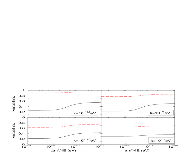
Figure 1: Neutrino survival probabilities, the solid line is $P_{ee}$, the dashed is the sum $P_{ee}+P_{e\mu}$, and the $P_{e\bar{\tau}}$ is the remaining until the maximum. We used $\tan^{2}\theta=0.4$ in all panels.

Now we are in condition to compute the $P_{1e}^{conv}$ and $P_{2e}^{conv}$ probabilities. In the convective region, the regular magnetic field is too small to induce spin-flip conversion and then the elements $h_{6}$ and $h_{7}$ vanishes. Then the Eq. (37) decouples in a sub-sector containing only $(\rho_{1},\rho_{2},\rho_{3},\rho_{8})$ elements as follows:

$${\frac{\displaystyle{\ d}}{\displaystyle{\ dt}}}\left(\begin{array}[]{c}\rho_{1}\\ \rho_{2}\\ \rho_{3}\\ \rho_{8}\end{array}\right)= \left(\begin{array}[]{cccccccc}-2k&-2h_{3}&0&0\\ 2h_{3}&-2k&-2h_{1}&0\\ 0&2h_{1}&-2k&2\sqrt{3}k\\ 0&0&2\sqrt{3}k&-6k\\ \end{array}\right)\left(\begin{array}[]{c}\rho_{1}\\ \rho_{2}\\ \rho_{3}\\ \rho_{8}\end{array}\right).$$ (53)

It is interesting to note that the evolution equation does not depend on $h_{8}$, not depending therefore on the atmospheric mass scale $\Delta m_{32}^{2}$. This is an important feature of our configuration, since as mentioned in the last section, the condition of validity of our equation is that the coherence length is smaller then the neutrino oscillation length.

At the bottom of convective zone the initial conditions are

$$\nu_{1} : \rho_{0}(0)=1/3,\,\,\rho_{1}(0)=-\sin{2\theta}/2,\,\,\rho_{3}(0)=\cos{2\theta}/2,\,\,\rho_{8}(0)=1/(2\sqrt{3})$$

$$\nu_{2} : \rho_{0}(0)=1/3,\,\,\rho_{1}(0)=\sin{2\theta}/2,\,\,\rho_{3}(0)=-\cos{2\theta}/2,\,\,\rho_{8}(0)=1/(2\sqrt{3})$$ (54)

To study the anti-neutrino production, we solve numerically Eq. (53) for different values of $k$, and with initial conditions given by the usual MSW mechanism in the radiative zone.

The effect of the random magnetic field inclusion in evolution equation can be seen in Fig. 1, where we can read the fraction of the different neutrino flavors, $\nu_{e}:\nu_{\mu}:\bar{\nu}_{\tau}$. The solid line represents the electronic neutrino survival probability, $P_{ee}$, while the dashed line is the $\nu_{e}+\nu_{\mu}$ fraction, $P_{ee}+P_{e\mu}$ The remaining until the no-oscillation value is the contribution of the $P_{e\bar{\tau}}$ probability. In all panels we used $\tan^{2}\theta=0.4$.

For small values of $k$, the electronic and muonic neutrinos start to convert into $\bar{\nu}_{\tau}$, and, as a consequence, the electronic survival probability decreases. For large values of $k$, the neutrino flux tends to split equally in the three neutrinos flavors, with $~{}1/3$ of the total flux for each flavor.

Taking the marginal allowed value of $L_{0}=10$ km, in order to have $k=10^{-14}$ eV as in the last panel of Fig. 1, we should have $B\sim 10$ MG, which is hardly acceptable. Lower values of neutrino energy will decrease the neutrino oscillation length, making it more difficult to fulfill the conditions in Eq. (38). In this sense, the values of $k=10^{-15}$ eV seems more feasible in a realistic scenario.

However, as pointed out in Section II, we expect that the effects of neutrino conversion would be stronger when $\lambda_{\nu}\sim L_{0}$. So the limitations expressed in the last paragraph are only numerical limitations, and not physical constraints. Having this in mind, we decided to extend the analysis up to $k=10^{-14}$ eV, assuming that a complete numerical integration of Eqs. (37) and (39) would give qualitatively the same results as we present here.

III LMA region

The validity of our numerical treatment is energy dependent, so we have made the choice to limit our fit to solar neutrino data to a specific neutrino energy range. Since the validity of our approximations may not hold for low energy neutrinos, we included only the data for the high energy neutrino (SNO-I, SNO-II and SK). We must be careful in analyzing allowed regions for neutrino parameters, since the inclusion of low energy solar neutrino data should change this picture.

The effect of the random magnetic field in the LMA region can be seen in Fig. 2. As the parameter $k$ increases, the electronic survival probability decreases. This effect can be compensated by a higher value of neutrino mixing angle, moving the allowed region to the right in left panel of Fig. 2.

For larger values of $k$, all probabilities tend to $~{}1/3$, with a weak dependence of the mixing angle. Since the Super-Kamiokande and SNO results are in accordance with this probability, in this scenario even maximal mixing is allowed. But also a interesting phenomenon occurs. Now a significant part of the total neutrino flux does not take part in regeneration effect in Earth. Actually, if we have exactly a equally equipartition of $\nu_{e}$, $\nu_{\mu}$ and $\bar{\nu}_{\tau}$ fluxes the regeneration effect vanishes, regardless of the neutrino mass difference $\Delta m^{2}$.

The right panel of Fig. 2 presents the KamLAND allowed regions, for $95\%$ C.L., $99\%$ C.L. and $3\sigma$. Maximal mixing is allowed at $62.1\%$ C.L., and low values of $\Delta m^{2}$ are still consistent with data at $99\%$ C.L.. This last region is inconsistent with solar neutrino experiments because it predicts a too strong regeneration effect, not seen by data.

In the present context, the regeneration effect can be suppressed for large values of $k$. As a result, lower values of $\Delta m^{2}$ are allowed, and a new region of compatibility between solar and KamLAND data appears. In other contexts of non-standard neutrino physics Guzzo:2003xk ; Guzzo:2004ue , we have called this region very-low LMA.

In Fig. 3 we present the allowed region for a combined analysis of high-energy solar neutrino and KamLAND data. We can see in this plot both the displacement of the allowed region to higher values of $\tan^{2}\theta$ for moderate values of $k$, and the appearance of the very-low LMA region at $\Delta m^{2}\sim[1-2]\times 10^{-5}$ eV² for $k=10^{-14}$ eV.

,

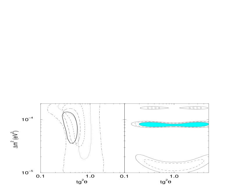
Figure 2: The LMA compatibility region for SNO+SK data (left panel) and the KamLAND allowed region (right panel). In left panel, the black line stands for no magnetic field, the long-dashed line for $k=10^{-15.5}$, the short-dashed line for $k=10^{-15}$, the dotted line for $k=10^{-14.5}$ and the dot-dashed line for $k=10^{-14}$. In the right panel the allowed regions stands for 95% C.L., 99% C.L. and 3$\sigma$ for respectively the filled, dashed and black curves.

,

Figure 3: Combined result for SNO+SK and KamLAND data, at 99% C.L., for the same values of $k$ presented in Fig. 2. Maximal mixing is allowed for $k>10^{-14.5}$.

IV $\theta_{13}\neq 0$

In this work, we assumed $\theta_{13}=0$, since non-vanishing values of this angle will lead to a production of $\bar{\nu}_{e}$, which is strongly constrained by data. Then, if $\theta_{13}\neq 0$ a limit in $\mu_{23}$ could be established in the same way the limits of the other components of magnetic moments were found Miranda:2003yh , in a two families analysis, denoted here by $\mu_{\nu}^{2fam}$.

Including the angle $\theta_{13}$ in the mixing matrix would lead to the term $\mu_{\nu}\sin\theta_{13}$ connecting $\bar{\nu}_{e}$ to the active neutrino families. So the limits in $\mu_{\nu}^{2fam}$ could be scaled to a limit in $\mu_{23}$ if a positive measurement of $\theta_{13}$ is achieved in the next round of reactor reactor13 and accelerator accelerator experiments. This limit would be weaker then the present limits in $\mu_{\nu}^{2fam}$ by a factor $1/\sin\theta_{13}$.

V Conclusions

We have investigated new effects in solar neutrino phenomenology due to interactions of these particles with a random solar magnetic field. Considering the context of LMA realization of the MSW solution to the solar neutrino anomaly we have analysed the neutrino spin-flavor conversion phenomenon which appears as a subleading effect when a non-vanishing neutrino magnetic moment linking the second and the third families is assumed. Such a magnetic moment induces a large conversion of solar neutrinos into non-electron anti-neutrino flux, which is not severely constrained by the solar neutrino observations.

Since the mixing angle $\theta_{13}$ can be considered very small, this conversion is not followed by a production of electron anti-neutrinos flux which, in contrast to non-electron anti-neutrinos, is very constrained by data.

The results of our analyses of SNO+SK compatibility region indicate that in the presence of solar random magnetic fields the allowed region for $\Delta m^{2}$ becomes larger while higher values of $\theta_{12}$ are found.

This is a consequence of the fact that, in a three neutrino family context, an electron-neutrino survival probability of $P~{}\sim 1/3$ is possible, even for $\tan^{2}\theta_{12}\sim 1$. In fact, when the random components of the solar magnetic field is large enough in such way that $k=10^{-14}$, values around $\Delta m^{2}\approx 10^{-5}$eV² are included in the region allowed by solar neutrino observations. Furtermore, different proportion of neutrinos and anti-neutrinos suppresses the regeneration effect of the solar neutrinos crossing the Earth matter. As a consequence, a totally new region of compatibility between solar neutrinos and KamLAND, which we call very-low LMA, appears at 99% C.L. for small values of $\Delta m^{2}_{21}\sim[1-2]\times 10^{-5}$ eV² and maximal mixing.