Effective Hamiltonian for QCD evolution at high energy

Abstract

We construct the effective Hamiltonian which governs the renormalization group flow of the gluon distribution with increasing energy and in the leading logarithmic approximation. This Hamiltonian defines a two–dimensional field theory which involves two types of Wilson lines: longitudinal Wilson lines which describe gluon recombination (or merging) and temporal Wilson lines which account for gluon bremsstrahlung (or splitting). The Hamiltonian is self–dual, i.e., it is invariant under the exchange of the two types of Wilson lines. In the high density regime where one can neglect gluon number fluctuations, the general Hamiltonian reduces to that for the JIMWLK evolution. In the dilute regime where gluon recombination becomes unimportant, it reduces to the dual partner of the JIMWLK Hamiltonian, which describes bremsstrahlung.

SACLAY–T05/057
BNL–NT–05/11

1 Introduction

The construction of an effective field theory for scattering in QCD at high energy is a difficult, longstanding, problem, which has been at the heart of theoretical developments for more than twenty years. In the ‘leading logarithmic approximation’ (LLA) which is expected to control the high–energy limit, the effective action should include the quantum effects enhanced by the large energy logarithm $\tau\equiv\ln s/Q^{2}$ (the ‘rapidity’; as usual, $s$ denotes the invariant total energy squared, and $Q$ is the typical momentum transfer, or a particle mass), that is, it must resum radiative corrections of order $(\alpha_{s}\ln s/Q^{2})^{n}$ to all orders. If this is the only requirement, then the corresponding resummation is performed by the Balitsky–Fadin–Kuraev–Lipatov (BFKL) equation [1], which is however well known to violate unitarity in the high energy limit: the corresponding solution for the scattering amplitudes or for the gluon distribution grows like a power of the energy, in violation of the Froissart bound. According to the modern understanding, the BFKL equation should govern only the pre–asymptotic evolution, at intermediate values of the energy. The complete effective action valid in the high energy limit should unitarize the BFKL ‘pomeron’ via the inclusion of multiple scattering. Alternatively, and equivalently, if the effective theory is written for the wavefunctions of the hadronic systems which participate in the collision (the ‘target’ and the ‘projectile’), the effective action must include the non–linear effects, like gluon recombination, responsible for gluon saturation [2, 3, 4, 5].

The first attempt towards constructing such an action has been given in Ref. [6], where the main arguments rely on kinematical and symmetry considerations. A lasting conclusion of this analysis is that the effective action should describe a two–dimensional field theory living in the plane transverse to the collision axis, and that the basic degrees of freedom should be Wilson line — path–ordered eikonal phases describing multiple scattering at high energy. The effective theory proposed in Ref. [6] involves two types of such Wilson lines, each of them describing the scattering of one of the participants in the collision off the color field created by the other participant. Subsequently, Lipatov and collaborators [7, 8] proposed an effective theory formulated in terms of reggeized gluons which contains the results in Ref. [6] as a special limit. More recently, Balitsky [9] has relied on a new factorization scheme (in rapidity) to construct an effective action in terms of Wilson lines, which extends the original construction in Ref. [6]. Some of his results will also emerge from our subsequent calculations. The direct comparison between the effective theory by Lipatov et al [7, 8] and that by Balitsky (or, more generally, any effective theory built in terms of Wilson lines, like the one to be developed below in this paper) is hindered by the fact that the general relation between the reggeized gluons and the usual gluon fields (and hence the Wilson lines) is not known.

However, all the approaches mentioned above have merely considered the effective action corresponding to a given layer in rapidity : The action is obtained by integrating out gluon fluctuations with rapidity $\tau$ within some intermediate range $\tau_{0}<\tau<\tau_{1}$, to leading order in $\alpha_{s}(\tau_{1}-\tau_{0})$ and under the assumption that $\alpha_{s}(\tau_{1}-\tau_{0})\ll 1$, in order for perturbation theory to apply. (The rapidity of a parton fluctuation is defined, as usual, as $\tau=\ln 1/x$, where $x$ is the longitudinal momentum fraction carried by that parton.) From the point of view of the leading logarithmic approximation, this represents a single evolution step (in the presence of multiple scattering, though), but in order to study the high energy behavior one really needs to iterate this step. To that aim, one should be able to promote the effective action into a (field theoretical) renormalization group Hamiltonian which should describe the evolution of the effective theory with increasing $\tau$. In turn, this requires the proper identification of the relevant degrees of freedom and of the way that these are changed by the evolution in each rapidity step.

Alternatively, the renormalization group (RG) flow can be formulated as an hierarchy of evolution equations for the relevant gluon correlation functions, which should reduce to the BFKL equation in the intermediate–energy regime where unitarity corrections are unimportant. Such an hierarchy has been derived for the first time by Balitsky [10]. This is an hierarchy for the evolution of Wilson–line operators which physically describe the scattering between a projectile made of elementary color charges (each of them identified by its own Wilson line) and the strong ‘background’ field of a target which is not evolving (like a large nucleus). The evolution consists in gluon splitting within the projectile wavefunction, followed by the multiple scattering between the products of this splitting and the background field. With increasing $\tau$, the gluon density in the projectile wavefunction is rapidly increasing, yet this formalism does not allow for non–linear effects like gluon recombination, which on physical grounds are expected to tame this growth.

The interpretation of Balitsky equations as an RG flow has been clarified by Weigert [11], who noticed that the hierarchy in Ref. [10] can be compactly reformulated as a single, functional, evolution equation for a classical probability distribution for the Wilson lines. The functional differential operator in this equation plays the role of a Hamiltonian; it involves only one type of Wilson line (since the scattering is asymmetric: the target is dense and produces a strong color field, while the projectile is dilute), together with functional (Lie) derivatives with respect to these Wilson lines. A posteriori, one can recognize Weigert’s Hamiltonian as a ‘quantized’ version of the effective action proposed by Balitsky for asymmetric scattering [10], where by ‘quantization’ we mean that the weak fields associated in the effective action with the projectile are replaced by functional Lie derivatives with respect to the Wilson lines built with the field of the target.

Independently, a different RG approach aiming at the description of the gluon distribution of a highly evolved hadronic system has been developed in Refs. [5, 12, 13, 14, 15] and has eventually crystalized into an effective theory for gluon correlations at small $x$ known as the color glass condensate (CGC) [15] (see also the review papers [16]). Following the general idea of the separation of scales in rapidity, this approach focuses on the evolution of a single hadron wavefunction (say, the target), with the purpose of integrating out the ‘fast’ quantum fluctuations — those with large longitudinal momenta — in layers of rapidity and thus obtain an effective theory for the correlations of the ‘soft’ (i.e., small–$x$) gluons, as probed in a high energy collision. The Wilson lines appear naturally also in this approach: They describe the multiple scattering between the quantum gluons to be integrated out in the next evolution step and the strong color fields generated by ‘color sources’ representing the fast gluons which have been integrated out in the previous steps.

The central result in the CGC approach is the Jalilian-Marian–Iancu–McLerran–Weigert–Leonidov–Kovner (JIMWLK) equation [14, 15], a functional RG equation which turns out to be equivalent [15, 17] with the equation deduced by Weigert [11] from the Balitsky hierarchy [10]. This equivalence reflects the fact that both approaches include the same physical non–linear phenomena, which are treated either as recombination effects in the target wavefunction (in the CGC approach) or as gluon splitting in the projectile wavefunction followed by multiple scattering off the target (in the approach by Balitsky). However, both approaches miss the other side of the problem, namely the saturation effects in the evolution of the projectile (for the Balitsky equations) and, respectively, the correlations associated with gluon splitting in the target wavefunction (in the case of the JIMWLK equation). Because of that, both approaches miss the ‘pomeron loops’, as first recognized in Ref. [18]. These are the loops which open up with vertices for gluon splitting (so like $2\to n$ with $n\geq 3$) in the dilute regime and close through vertices for gluon merging (e.g., $n\to 2$) in the high density regime. (The denomination ‘pomeron loops’ is strictly correct only in the limit where the number of colors $N_{c}$ is large and the $t$–channel gluons can be pairwise combined into BFKL pomerons, but here we use this expression as a convenient short–cut also for the general case at arbitrary $N_{c}$.)

The gluon splitting and merging vertices in the high–energy evolution are generalizations of the $2\to 2$ BFKL vertex in the Lipatov Hamiltonian [19]. Such vertices have been explicitly computed in perturbative QCD [20, 21, 22, 23, 24] (see [25] for a review) and appear implicitly as building blocks in the Balitsky and JIMWLK equations, from which they can be in principle extracted by expanding the Wilson lines in powers of the gauge fields. However, until recently the only formalism allowing for the simultaneous inclusion of both splittings and mergings in a high–energy scattering was Mueller’s center–of–mass factorization of onium–onium scattering [26, 27, 28]. In this approach, the gluon splittings are included in the evolution of the wavefunctions of the two onia (described as evolving distributions of quark–antiquark ‘color dipoles’, as appropriate at large $N_{c}$), while the mergings are represented by multiple scattering (the simultaneous scattering of several pairs of dipoles from the two onia). The numerical simulations of the onium–onium scattering by Salam [29] have demonstrated the importance of the correlations induced by gluon splitting, whose physical role has been fully understood only recently [30, 31, 32]: the gluon number fluctuations act as a seed for higher–point correlations in the dilute regime, and thus strongly influence the evolution towards high density.

The first evolution equations in QCD to take into account both mergings and splittings have been proposed in Ref. [18] and shortly after improved in Refs. [33, 34]. These equations generalize Balitsky equations at large $N_{c}$ by including the effects of gluon number fluctuations within the framework of the color dipole picture. By construction, these equations describe dipole evolution (including dipole number fluctuations) in the dilute regime and JIMWLK–like gluon recombination in the high–density regime, and thus contain all the necessary ingredients to provide a complete picture of the evolution at large $N_{c}$ and for sufficiently high energies. The RG formulation of these equations is also explicitly known [33, 35]: this involves an effective Hamiltonian which describes a two–dimensional field theory for the dynamics of ‘Pomerons’ [35]. In this context, the ‘Pomerons’ represent color singlet exchanges in the scattering between a dipole and a generic target. With increasing $\tau$, the Pomerons undergo BFKL evolution, they can dissociate (one Pomeron splitting into two) or recombine with each other (two Pomerons merging into one). This effective theory has a remarkable symmetry which reflects boost invariance: It is invariant under the duality transformations which exchange color fields with the functional derivative with respect to these fields (or, more precisely, with respect to their sources). Under these transformations, the splitting and mergings terms in the Hamiltonian get interchanged with each other, while the BFKL piece is self–dual.

Whereas for large $N_{c}$, the high–energy evolution in QCD is by now well understood [18, 34, 33, 36, 35, 37], its generalization to finite $N_{c}$ remains an outstanding open problem, which is actively under investigation [38, 39, 40]. Recently, Kovner and Lublinsky [38] have constructed evolution equations for gluon correlations in the dilute regime valid for arbitrary $N_{c}\,$, and then noticed [39] that the effective Hamiltonian generating these equations — to which we shall refer as the bremsstrahlung (BREM) Hamiltonian in what follows — is in fact dual to the JIMWLK Hamiltonian [11, 15]. Following this idea, they made the interesting suggestion [39] that the general (and yet unknown) evolution Hamiltonian, which describes both mergings and splittings, should be self–dual as a consequence of boost invariance. But in the absence of an explicit derivation of this Hamiltonian from the QCD Feynman rules, the hypotheses in Ref. [39] are difficult to test. Besides, by itself, the duality argument does not allow one to construct the general Hamiltonian for the QCD evolution, but only to relate its limiting expressions in the dense and dilute regimes.

In fact, related work by the same authors [38, 40] shows that the extension of the JIMWLK equation to the dilute regime is afflicted with difficulties associated, in particular, with ambiguities due to the time–ordering of the correlations induced by quantum evolution. At this point, one should recall that previous formalisms like the CGC approach and the Balitsky equations, and also the effective action approaches in Refs. [6, 7, 8, 9], have been specially tailored to deal with the high density, or strong field, regime, as relevant in the vicinity of the unitarity limit, but they need not be well suited for the description of subtle correlations induced by fluctuations in the dilute regime. Thus, in view of the current understanding, the very existence of a general evolution Hamiltonian which encompasses all the desired phenomena is far from being clear, and the actual expression of this Hamiltonian, if any, is completely unknown.

It is our main objective in this paper to investigate under which conditions the renormalization group approach developed in Refs. [14, 15] can be extended to account for gluon splitting in addition to gluon recombination, and thus promoted into a general theory for QCD evolution in the LLA. As we shall see, such an extension can be given indeed, but only within the limitations inherent to an RG analysis, which implies a coarse–graining as usual. Here, the ‘coarse–graining’ refers, of course, to rapidity, and thus to the longitudinal and temporal scales simultaneously. The effective theory can capture only those correlations that can be ‘seen’ by the quantum fluctuations which are integrated out in one step of the evolution. As we shall briefly explain here (and then demonstrate at length in the main body of the paper), such correlations are fully encoded in two types of Wilson lines — path–ordered exponentials in the longitudinal and, respectively, temporal direction — which with increasing $\tau$ evolve through gauge rotations at their end points.

Indeed, one step of quantum evolution consists in integrating out ‘semi–fast’ gluon fluctuations in a rapidity layer $\tau_{0}<\tau<\tau_{1}$ and in the presence of two types of background fields: the ‘fast’ fields created by the gluons with larger longitudinal momenta that have been integrated out in the previous steps, and the ‘slow’ fields radiated by the ‘semi–fast’ gluon itself. The multiple scattering off the ‘fast’ background fields accounts for gluon merging, whereas the simultaneous emission of several ‘slow’ fields implements gluon splitting (or bremsstrahlung). The resolution scales of the semi–fast gluon are fixed by the light–cone kinematics together with the separation of scales: This gluon has a poor resolution both on the longitudinal scale characteristic for the fast fields and on the temporal scale characteristic for the slow ones. Thus, it can only measure an ‘integrated’ effect of these fields, and since this measure proceeds via multiple scattering, its result is encoded in Wilson lines. The supports of the longitudinal and temporal integrations implicit in the Wilson lines are evolving with $\tau$, but the background fields change only at the extremities of these supports, so the Wilson lines change only at their end points (where new correlations are induced by the quantum evolution).

The effective Hamiltonian that we shall obtain is a functional of these two types of Wilson lines, and is moreover self–dual : that is, it is invariant under the exchange between longitudinal and temporal Wilson lines. This invariance reflects a mirror symmetry between vertices for gluon splitting and, respectively, gluon merging, which is in turn related to the boost invariance of the evolution equations. In the limiting regimes where one of the background fields is weak (so that the corresponding Wilson lines can be expanded out in perturbation theory), the general Hamiltonian reduces to the expected limiting forms: (i) at high density, where the gluon number fluctuations become negligible, it reduces to the JIMWLK Hamiltonian [11, 15]; (ii) at low density, where gluon recombination can be ignored, it reduces to the bremsstrahlung Hamiltonian [39], which is dual to the JIMWLK Hamiltonian, in agreement with Ref. [39].

For each of the two limiting situations alluded to above (JIMWLK and BREM), the two–dimensional Hamiltonian structure is explicit and transparent: the canonical variables and the associated conjugate momenta are properly identified, and the corresponding Poisson brackets are explicitly known. Note that these Poisson brackets are non–trivial, in the sense that some of the variables — those associated with the weak fields and which play the role of Lie derivatives — are non–commutative: they do not commute with themselves, but rather obey the SU($N_{c}$) current algebra. The evolution equations are then obtained as the canonical equations of motion generated by the respective Hamiltonian via the Poisson brackets. For the JIMWLK Hamiltonian this procedure yields the Balitsky equations [10], as usual, whereas for the BREM Hamiltonian it leads to equations similar to those written down by Kovner and Lublinsky [38].

But precisely because of the lack of commutativity alluded to above, we have not been able to extend the construction of the Poisson brackets to the general case, where both types of background fields are strong. The would–be straightforward construction, which consists in exponentiating the Lie derivatives, leads to non–local commutation relations, which reintroduce the longitudinal and temporal coordinates, and thus are unacceptable. The completion of the Hamiltonian structure in the general case is left for further studies.

This paper will be organized as follows: In Sect. 2 we shall describe the scattering problem that we have in mind and its formulation in the CGC formalism. This will also give us the opportunity to introduce some notations and fix our conventions. In Sect. 3 we shall explain the general philosophy of the RG approach underlying the effective theory for the CGC. The discussion will be mostly qualitative, with the aim of anticipating and thus clarifying the physical interpretation of the subsequent, more technical, developments. The next two sections will provide the mathematical formulation of the RG: In Sect. 4 we shall derive general formulae for the effective action encoding the correlations induced after one step in the quantum evolution. The action is manifestly gauge–invariant and is expressed in terms of the background field propagator for the semi–fast gluons, that we shall construct (within the approximations and for the physical regime of interest) in Sect. 5. The self–duality will appear already in Sect. 4, as a symmetry relating two different, but equivalent, expressions for the effective action. The first application of the general formalism will be given in Sect. 6, where we shall provide a streamlined derivation of the JIMWLK Hamiltonian. This derivation is considerably shorter then the previous ones in the literature [14, 15], thus demonstrating the efficiency of the present formulation of the RG. Then, in Sect. 7 we turn to the general case and construct the effective action as a functional of the two types of Wilson lines. We shall derive four different, but equivalent, versions for this action. The self–duality is now manifest, as the invariance of the action under the exchange between longitudinal and temporal Wilson lines. We shall also check that the JIMWLK action is indeed obtained from the general action in the limit where fluctuations become negligible. Finally, in Sect. 8 we consider the limiting case of a dilute regime and thus deduce the Hamiltonian for bremsstrahlung. We construct the associated Poisson brackets and explain how to use them in order to derive evolution equations for observables like the scattering amplitudes. Sect. 9 contains our conclusions.

2 The scattering problem in the CGC formalism

Let us start with a description of the scattering problem that we have in mind. We shall consider a high energy scattering in which the target is a right–mover (it propagates in the positive $z$, or positive $x^{+}$, direction), whereas the projectile is a left–mover (it propagates towards negative $z$, or positive $x^{-}$). Note that, for the target, $x^{+}$ plays the role of time and $x^{-}$ that of the longitudinal coordinate, while for the projectile the roles of $x^{+}$ and $x^{-}$ are interchanged. Furthermore, we shall view the scattering in a Lorentz frame in which the target carries most of the total energy, so that its wavefunction is highly evolved — it contains many small–$x$ gluons — and can be described as a color glass condensate (see below). In that frame, the projectile is a relatively simple object, like a quark–antiquark pair in a colorless state (a ‘color dipole’), or a collection of several such dipoles.

Since the gluon density in the target is typically high, the projectile will undergo multiple scattering, which can be resummed in the eikonal approximation: A quark (or antiquark) which propagates through the target preserves a straightline trajectory but acquires a color precession; that is, its wavefunction gets multiplied by a Wilson line built with the projection of the color field of the target along the trajectory of the quark. For a left–moving quark with transverse coordinate $\bm{x}$, this Wilson line reads :

$$V^{\dagger}(\bm{x})={\mbox{P}}\exp\left\{ig\int dx^{-}A^{+}_{a}(x^{+}\simeq 0,x^{-},\bm{x})\,t^{a}\right\}\,,\vspace{-.5cm}$$ (2.1)

where the $t^{a}$’s are the generators of the SU$(N_{c})$ algebra in the fundamental representation and the symbol P denotes the $x^{-}$ ordering of the color matrices $A^{+}_{a}(x^{-})t^{a}$ in the exponent, from right to left in increasing order of their $x^{-}$ arguments. The integration runs formally over all the values of $x^{-}$, but in reality it is restricted to the longitudinal extent of the target, which is localized near $x^{-}=0$ because of Lorentz contraction. By the same argument, the projectile is localized near $x^{+}=0$, so it probes the target field $A^{+}$ at small $x^{+}$, as also indicated on Eq. (2.1).

In fact, the field $A^{+}$ is slowly varying in $x^{+}$, since it is generated by fast moving color sources — the quarks and gluons inside the target — whose internal dynamics is slowed down by Lorentz time dilation. Thus, the target field can be treated as constant over the duration of the scattering. This motivates the color glass picture to be developed below, in which the scattering observables are first computed for a given configuration of the color fields in the target, and then averaged over the latter.

Specifically, the $S$–matrix for the scattering between a color dipole and the color field $A^{+}$ is obtained as the color average of the product of two Wilson lines: one for the quark and the other one for the antiquark (with transverse coordinates $\bm{x}$ and $\bm{y}$, respectively) :

$$S(\bm{x},\bm{y};A^{+})\,=\,\frac{1}{N_{c}}\,{\rm tr}(V^{\dagger}_{\bm{x}}V_{\bm{y}}).\vspace{-.5cm}$$ (2.2)

The physical $S$–matrix for dipole–hadron scattering is finally obtained after averaging over all the configurations of the color fields $A^{+}$ in the target. Within the CGC effective theory, this average is computed as follows:

$$\langle S(\bm{x},\bm{y})\rangle_{\tau}\,=\,\frac{1}{N_{c}}\big{\langle}{\rm tr}(V^{\dagger}_{\bm{x}}V_{\bm{y}})\big{\rangle}_{\tau}\,\equiv\,\int D[\rho]\,\,{\cal W}_{\tau}[\rho]\,\frac{1}{N_{c}}\,{\rm tr}(V^{\dagger}_{\bm{x}}V_{\bm{y}}).\vspace{-.5cm}$$ (2.3)

This formula makes it explicit that the field $A^{+}$ is created by ‘color sources’ (quantum fluctuations in the target wavefunction) with large longitudinal momenta $k^{+}$, whose lifetimes are much larger than the collision time. In the computation of scattering amplitudes, these sources can be effectively replaced by a classical color current $J^{\mu}_{a}=\delta^{\mu+}\rho_{a}$, where the charge density $\rho_{a}\equiv\rho_{a}(x^{-},\bm{x})$ is static, i.e., independent of $x^{+}$, but random, as it corresponds to any of the possible configurations of the fast moving partons. The correlations of $\rho$ are encoded in the weight function ${\cal W}_{\tau}[\rho]$ — a functional probability distribution which depends upon the target rapidity $\tau\sim\ln s$ because of quantum evolution :

The fast partons which represent the color sources have longitudinal momenta within the range $P^{+}\gg k^{+}\gg\Lambda$, where $P^{+}$ is the total momentum of the target and $\Lambda$ is the scale at which the lifetime of a virtual excitation becomes of the order of the collision time. When increasing the energy $s$ of the collision, $P^{+}$ increases like $\sqrt{s}$, while $\Lambda$ remains constant (since this is fixed by the properties of the projectile). Thus, the longitudinal phase–space $P^{+}\gg k^{+}\gg\Lambda$ available for quantum evolution is increased, leading to an enhanced gluon radiation, and thus to the generation of new color sources. The effects of this evolution will be discussed in detail and computed in the next sections.

In particular, in the dilute regime at not so high energies, the target field is weak and Eq. (2.2) can be evaluated by expanding the exponentials in the Wilson lines. To lowest non–trivial order in this expansion one obtains the scattering amplitude in the two–gluon exchange (or single scattering) approximation:

$$T(\bm{x},\bm{y})\equiv 1-S(\bm{x},\bm{y})\,\simeq\,\frac{g^{2}}{4N_{c}}\,(A^{+}_{a}(\bm{x})-A^{+}_{a}(\bm{y}))^{2}\,,\vspace{-.5cm}$$ (2.4)

where

$$A^{+}_{a}(\bm{x})\,\equiv\,\int dx^{-}\,A^{+}_{a}(x^{+}=0,x^{-},\bm{x})\vspace{-.5cm}$$ (2.5)

is the effective color field in the transverse plane, as obtained after integrating over the longitudinal profile of the target. Note that the ordering of the Wilson lines in $x^{-}$ plays no role in this approximation, because of the symmetry of the color trace: ${\rm tr}(t^{a}t^{b})=\frac{1}{2}\,\delta^{ab}={\rm tr}(t^{b}t^{a})$. However, this ordering does matter in the strong field regime in which multiple scattering is important and the complete equation (2.2) must be used: successive collisions do not commute with each other (as they involve color matrices), so they resolve the longitudinal structure of the color field in the target. Thus in the construction of the effective theory one should also keep trace of the correlations of the color sources in $x^{-}$. But in the approximations of interest at high energy, these correlations turn out to be relatively simple and can always be embedded via Wilson lines. In particular, the effective theory and its evolution can be fully written in terms of Wilson lines [10, 11], in which case the longitudinal coordinate $x^{-}$ is not explicit anymore.

3 Quantum evolution: The general philosophy

In this section we shall explain the general structure of the quantum evolution and describe our strategy towards performing the calculation. This strategy relies on the renormalization group (RG) in QCD at small–$x$, a technique which allows one to integrate out quantum fluctuations in the evolution with increasing energy by exploiting the separation of (longitudinal and temporal) scales specific to the high–energy problem. This technique generalizes the BFKL evolution [1] and has been originally developed in Refs. [14, 15] in relation with the JIMWLK equation. In what follows we shall further develop this technique and apply it to the construction of more general evolution equations, from which the JIMWLK equation will emerge as a special limit. The discussion in this section is purely qualitative: we shall explain the structure of the quantum corrections and emphasize some general properties which will facilitate the physical interpretation of the calculations in the next sections. We shall thus anticipate from physical considerations some structural properties of the evolution equations that will be later confirmed by explicit calculations.

As explained in the previous section, our objective is to construct an effective theory for gluon correlations in the target wavefunction at some soft longitudinal momentum scale $\Lambda$ with $\Lambda\ll P^{+}$. For instance, to compute scattering amplitudes at the scale $\Lambda$, we need $n$–point functions like $\langle A^{+}(x)A^{+}(y)\cdots\rangle_{\Lambda}$, where the subscript $\Lambda$ means that the fields $A^{+}$ inside the brackets carry soft longitudinal momenta $k^{+}\sim\Lambda$. At high energy, such soft fields are predominantly generated by relatively fast color sources, with longitudinal momenta $p^{+}$ such that $P^{+}\gg p^{+}\gg\Lambda$. Indeed, due to the infrared singularity of the bremsstrahlung spectrum $\propto dp^{+}/p^{+}$, the contribution of these sources to the correlations at scale $\Lambda$ will be enhanced by powers of the large energy logarithm $\ln(P^{+}/\Lambda)\sim\ln s$, and thus will dominate over the genuine quantum fluctuations with $k^{+}\sim\Lambda$. Therefore, in the leading logarithmic approximation (LLA) to which we shall restrict ourselves in what follows, the soft fields at scale $\Lambda$ are entirely generated by fast color sources with $p^{+}\gg\Lambda$ and inherit the correlations of the latter. To the same approximation, the relevant ‘color sources’ are gluons which are themselves radiated by other gluons with even larger longitudinal momenta. This separation of scales makes it natural to use an RG analysis in which the fast gluon fluctuations are integrated out in layers of $p^{+}$ and replaced by an effective color charge density $\rho_{a}(x^{-},\bm{x})$ which generates the same correlations as the quantum gluons at the soft scale $\Lambda$.

Before we describe the quantum evolution, let us briefly review the solution to the classical equations of motion which rely the soft fields to $\rho$ (this solution will be needed later). The relevant equations are the Yang–Mills equations with a source $J^{\mu}_{a}=\delta^{\mu+}\rho_{a}$ ,

$$(D_{\nu}F^{\nu\mu})_{a}(x)\,=\,\delta^{\mu+}\rho_{a}(\vec{x})\,,\vspace{-.5cm}$$ (3.1)

where $\vec{x}=(x^{-},\bm{x})$ and $D_{\nu}=\partial_{\nu}-igA_{\nu}^{a}T^{a}$ with $(T^{a})_{bc}=-if_{abc}$. Because of the relatively simple structure of the current in the r.h.s., these equations can be solved explicitly (at least in specific gauges). Namely, it is consistent with Eq. (3.1) to search for a solution having the following properties [16]

$$F^{ij}_{a}=0,\qquad A^{-}_{a}=0,\qquad A^{+}_{a},\,A^{i}_{a}\,:\,\,{\rm independent\ of\ }x^{+}\,.\vspace{-.5cm}$$ (3.2)

Then the only non–trivial field strength is $F^{+i}_{a}$. After also imposing a gauge condition, the classical solution involves just one independent field degree of freedom. This becomes manifest in the Coulomb gauge $\nabla^{i}\tilde{A}^{i}=0$, where Eq. (3.1) reduces to

$$-\nabla^{2}_{\perp}\widetilde{A}^{+}_{a}({\vec{x}})\,=\,{\widetilde{\rho}}_{a}(\vec{x})\,,\vspace{-.5cm}$$ (3.3)

which is the light–cone analog of the Poisson equation. Note that we use a tilde to denote the classical source and field in the Coulomb gauge. In fact, the Coulomb gauge potential will appear so often in what follows that it becomes convenient to introduce a shorter notation for it: $\widetilde{A}^{+}_{a}\equiv\alpha_{a}$. Eq. (3.3) is immediately solved as

$$\alpha_{a}(x^{-},\bm{x})=\int\frac{d^{2}\bm{y}}{4\pi}\,\ln\frac{1}{(\bm{x}-\bm{y})^{2}\mu^{2}}\,\widetilde{\rho}_{a}(x^{-},\bm{y})\,\equiv\int d^{2}\bm{y}\,\Delta(\bm{x}-\bm{y})\,\widetilde{\rho}_{a}(x^{-},\bm{y}),\vspace{-.5cm}$$ (3.4)

where the infrared cutoff $\mu$ is necessary to invert the Laplacian operator in two dimensions, but it will eventually disappear from the physical results. The field strength in this gauge is obtained as $\tilde{F}^{+i}_{a}\,=\,-\partial^{i}\widetilde{\alpha}_{a}$.

We shall also need later the classical solution in the light–cone (LC) gauge $A^{+}_{a}=0$. This is constructed from the above solution in the Coulomb gauge via a gauge rotation

$${A}^{i}(x^{-},\bm{x})\,=\,\frac{i}{g}\,U(x^{-},\bm{x})\,\partial^{i}U^{\dagger}(x^{-},\bm{x})\,,\vspace{-.5cm}$$ (3.5)

with

$$U^{\dagger}(x^{-},\bm{x})={\rm P}\exp\left\{ig\int_{-\infty}^{x^{-}}dz^{-}\,\alpha_{a}(z^{-},\bm{x})T^{a}\right\}.\vspace{-.5cm}$$ (3.6)

where we use matrix notations appropriate for the adjoint representation (${A}^{i}={A}^{i}_{a}T^{a}$, etc). Note the boundary condition: $A^{i}_{a}(x^{-},\bm{x})\to\,0$ for $x^{-}\to\,-\infty$.

Eqs. (3.4), (3.5), and (3.6) together provide an explicit expression for the LC–gauge solution ${A}^{i}$ in terms of the color source ${\tilde{\rho}}\,$ in the Coulomb gauge. Note that the target average in equations like (2.3) can be computed by using the classical solution in any gauge, since the measure, the weight function, and the physical observables are all gauge invariant.

We now return to the problem of the quantum evolution and start with the simplest case, that of the evolution of the 2–point function (2.4) in the dilute regime. In the LLA of interest, this evolution is described by the BFKL equation [1], and is schematically illustrated in Fig. 1.

Figure 1: The 2–point function in the effective theory (a) and its BFKL evolution in one step (b).

Fig. 1.a represents the 2–point function in the effective theory at scale $\Lambda$ : the color fields $A^{+}$ are radiated from the classical charge density $\rho$ and the average over $\rho$ (with weight function ${\cal W}_{\Lambda}[\rho]$) is represented by the upper blob. The one–step BFKL evolution of this 2–point function is represented in Fig. 1.a: this rung diagram is a typical quantum correction which becomes important when we probe correlations at the lower scale $b\Lambda$, with $b\ll 1$. These correlations have two sources: the direct emission of a gluon with $k^{+}\sim b\Lambda$ from the classical source at scale $\Lambda$ (cf. Fig. 1.a) and the induced radiation from the semi–fast quantum gluons with intermediate momenta $\Lambda\gg p^{+}\gg b\Lambda$ (the rung in Fig. 1.b). The quantum process gives a correction of order $\alpha_{s}\ln(1/b)$, and we shall assume that $\alpha_{s}\ln(1/b)\ll 1$ in order for perturbation theory to apply. The purpose of the renormalization group analysis is to replace the two contributions in Figs. 1.a and b by a single classical contribution similar to Fig. 1.a, but with a modified weight function ${\cal W}_{b\Lambda}[\rho]$. By computing the difference ${\cal W}_{b\Lambda}-{\cal W}_{\Lambda}\sim\alpha_{s}\ln(1/b)$, one can establish the renormalization group equation (RGE) whose solution permits to iterate an arbitrary number of evolution steps. Introducing the rapidity $\tau\equiv\ln(\Lambda/P^{+})$, so that $d\tau=\ln(1/b)$ for one step of RG, it is clear that $\tau$ plays the role of the evolution ‘time’.

It turns out that, quite generally, the RGE can be cast in Hamiltonian form, and can be applied either to the weight function

$$\frac{\partial}{\partial\tau}\,{\cal W}_{\tau}[\rho]=-H\Big{[}\rho,\frac{\delta}{i\delta\rho}\Big{]}{\cal W}_{\tau}[\rho]\,,\vspace{-.5cm}$$ (3.7)

or directly to the interesting observables, for example the dipole $S$–matrix (2.3)

$$\frac{\partial}{\partial\tau}\,\langle S[\rho]\rangle_{\tau}=-\Big{\langle}H\Big{[}\rho,\frac{\delta}{i\delta\rho}\Big{]}\,S[\rho]\Big{\rangle}_{\tau}\,,\vspace{-.5cm}$$ (3.8)

where $H$ is a Hermitian functional differential operator that we shall refer to as the ‘Hamiltonian’. By inspection of the diagrams in Fig. 1, it should be already clear what is the general structure of the BFKL Hamiltonian: When applied to a $n$–point function of the charge density $\rho$, this should annihilate two $\rho$’s and replace them by two new ones which interact with each other with the exchange of a BFKL rung. This suggests that

$$H_{\rm BFKL}\,=\,\frac{1}{2}\,\cal{K}_{\rm BFKL}\,\frac{\delta}{\delta\rho}\,\rho\,\rho\,\frac{\delta}{\delta\rho}\,,\vspace{-.5cm}$$ (3.9)

in schematic notations in which $\rho$ should be understood as the two–dimensional color charge density, obtained as in Eq. (2.5)

$$\rho_{a}(\bm{x})\,\equiv\,\int dx^{-}\,\rho_{a}(x^{-},\bm{x}).\vspace{-.5cm}$$ (3.10)

Indeed, there is no multiple scattering in the BFKL evolution, so the longitudinal structure can be trivially integrated out leaving a non–trivial dynamics in the transverse plane alone.

Note two important features of Eq. (3.9) which are more general than the BFKL approximation and will be recovered for the general equations below. First, the fact that the r.h.s. of Eq. (3.9) is a total derivative with respect to $\rho$ is necessary to ensure probability conservation: this guarantees that the normalization condition $\int D[\rho]\,{\cal W}_{\tau}[\rho]=1$ is preserved by the evolution. Second, note the specific ordering of the operators $\rho$ and ${\delta}/{\delta\rho}$ (which do not commute with each other) : this is obtained after subtle cancellations between ‘real’ and ‘virtual’ corrections in the quantum calculation (see e.g. Refs. [11, 15]), but is in fact imposed by gauge symmetry [41]. Thus, in order to obtain the evolution Hamiltonian, it is in fact sufficient to compute the real correction (so like the real gluon emission in Fig. 1.b) and then order the operators in such a way to ensure gauge symmetry. This is the strategy that we shall adopt in what follows.

Let us turn now to the more interesting case where the target field is strong (this is the typical situation at high energy). This entails non–linear effects both in the classical equations of motion (3.1) and in the quantum evolution. Indeed, in this case, the semi–fast gluon in Fig. 1.b propagates in the background of the strong classical field generated by the source $\rho$ at scale $\Lambda$ and undergoes multiple scattering off this field. Accordingly, the propagator of the semi–fast gluon must be computed to all orders in the background field. A typical diagram included in this resummation is shown in Fig. 2.a. Clearly, this describes gluon recombination : $n$ gluons (with $n\geq 2$) are merging into two. Such merging processes are responsible for the saturation of the gluon distribution and the formation of a color glass condensate.

In order to resum these processes to all orders, it is useful to notice that the kinematical conditions are satisfied for the use of the eikonal approximation . Indeed, as compared to the fast color sources responsible for the background field, the ‘semi–fast gluons’ are relatively slow. In the rest frame of the background field (which is the frame in which the eikonal approximation becomes most intuitive), the semi–fast gluons propagate in the negative $z$, or positive $x^{-}$, direction, so like the projectile in the scattering problem considered in the previous section. Therefore, the gluon propagator, and also the evolution Hamiltonian, will depend upon the background field via the same Wilson lines as in Eq. (2.1), except that these are now rewritten in the adjoint representation.

Figure 2: One–step quantum evolution with gluon number changing vertices: (a) a $n\rightarrow 2$ merging process which contributes to the JIMWLK Hamiltonian; (b) a $2\rightarrow n$ splitting process as included in the BREM Hamiltonian; (c) a general $m\rightarrow n$ process.

We thus see that, in the presence of non–linear effects, the quantum evolution is able to discriminate the longitudinal structure of the color source, so like the scattering with an external projectile. This brings us to the issue of the $x^{-}$ correlations generated by the quantum evolution. Because of the separation of scales in the problem, these correlations turn out to be quite trivial: they merely show that the color source $\rho_{a}(x^{-},\bm{x})$ extends towards larger values of $x^{-}$ when increasing $\tau$ [15]. Namely, by the uncertainty principle, the color source generated after integrating out the fast partons with momenta $p^{+}\gg\Lambda$ is localized near $x^{-}=0$ within a distance $\Delta x^{-}\sim 1/\Lambda$. With the boundary conditions that we shall use in our calculation, and which are the same as in Ref. [15], the support of the source lies fully at positive values of $x^{-}$, namely at $0\leq x^{-}\leq x^{-}_{\tau}$ with $x^{-}_{\tau}\sim 1/\Lambda=(1/P^{+}){\rm e}^{\tau}$. When a new layer of semi–fast gluons is integrated out, the additional color charge generated in this way is localized at $1/\Lambda\mathrel{\hbox to0.0pt{\raise 2.20013pt\hbox{$<$}\hss}{\lower 2.20013pt\hbox{$\sim$}}}x^{-}\mathrel{\hbox to0.0pt{\raise 2.20013pt\hbox{$<$}\hss}{\lower 2.20013pt\hbox{$\sim$}}}1/b\Lambda$, and thus has no overlap with the previously existing color source. Thus, the quantum evolution proceeds by adding new layers to the color source at larger values of $x^{-}$, whereas the charge density in the inner layers — as generated in the previous steps — is not modified. This means that the correlations induced by the evolution are essentially local in $x^{-}$ [17].

The previous discussion implies that, in a Wilson line like Eq. (2.1), the support of the integration is truly restricted to $0\leq x^{-}\leq x^{-}_{\tau}$ and, moreover, the net effect of increasing $\tau$ by $d\tau$ is an infinitesimal gauge rotation of the Wilson line at its large–$x^{-}$ end

$$V^{\dagger}_{\tau}({\bm{x}})=\,{\rm P}{\rm exp}\left\{ig\int_{0}^{x^{-}_{\tau}}dx^{-}\alpha(x^{-},\bm{x})\right\}\quad\longrightarrow\quad V^{\dagger}_{\tau+d\tau}({\bm{x}})=\,{\rm e}^{{\rm i}g\int dx^{-}\delta\alpha_{\tau}(x^{-},\bm{x})}\,V^{\dagger}_{\tau}({\bm{x}})\,,$$ (3.11)

where $\delta\alpha^{a}_{\tau}$ has support in the outer layer at $1/\Lambda\mathrel{\hbox to0.0pt{\raise 2.20013pt\hbox{$<$}\hss}{\lower 2.20013pt\hbox{$\sim$}}}x^{-}\mathrel{\hbox to0.0pt{\raise 2.20013pt\hbox{$<$}\hss}{\lower 2.20013pt\hbox{$\sim$}}}1/b\Lambda$, but its detailed $x^{-}$ dependence is irrelevant in the approximations of interest. Correspondingly, the functional derivatives in the RGE in the strong field regime are taken with respect to the color source (or field) in the outmost bin in $x^{-}$

$$H_{\rm JIMWLK}\,=\,\frac{1}{2}\,\frac{\delta}{\delta\alpha_{\tau}}\,\chi_{\rm JIMWLK}[V,V^{\dagger}]\,\frac{\delta}{\delta\alpha_{\tau}}\,.\vspace{-.5cm}$$ (3.12)

This is the JIMWLK Hamiltonian whose first complete derivation (including the subtle issue of the $\tau$–dependence of the functional derivatives) has been given in Ref. [15]. Mathematically, the functional derivatives which appear in Eq. (3.12) are really Lie derivatives with respect to the Wilson lines $V$ and $V^{\dagger}$ [17]. This is explicit in the independent derivation of the JIMWLK Hamiltonian by Weigert [11] from the Balitsky equations [10].

Thus, in this strong field regime, the evolution Hamiltonian is naturally expressed in terms of Wilson lines and functional derivatives with respect to the latter, and not directly in terms of the color source $\rho_{a}(x^{-},\bm{x})$. This is indeed the correct way to think about the high–energy evolution: as a renormalization group flow in a two–dimensional Hilbert space with a non–trivial geometry (namely, the group manifold spanned by the Wilson lines). On the other hand, given the separation of scales in the problem, one cannot address questions about the detailed longitudinal structure of the color source (like, e.g., computing correlations between the values of $\rho_{a}(x^{-},\bm{x})$ at different points $x^{-}$) : only the correlations of the Wilson lines make sense. We shall recover this feature in more general situations below.

Consider now the $2\rightarrow n$ splitting diagram in Fig. 2.b, in which the $n$ emerging gluons are all soft (i.e., they carry momenta $k^{+}\sim b\Lambda$). Physically, this diagram describes gluon bremsstrahlung in the process of the BFKL evolution. Through such processes, $n$–point correlation functions with $n>2$ get built from the 2–point function in the course of the quantum evolution. Gluon splitting has not been included in the analysis leading to the JIMWLK equation since formally this is a higher–order effect (as compared to the direct emission of $n$ gluons from the classical source $\rho$) in the strong field regime. However, this argument implicitly assumes that the higher correlations for $\rho$ have been already included in the weight function ${\cal W}_{\tau}[\rho]$. But when starting the evolution in the dilute regime (at low energy, or high transverse momenta), the higher–point correlations are originally absent, and they can only get built from the 2–point function. Thus, gluon splitting is in fact the dominant process for generating correlations in the dilute regime, and as such it has also a strong influence on the dynamics in the high–density regime, since the non–linear effects mix various correlations with each other, as obvious in Fig. 2.a.

Focusing on the dilute regime for the time being, we would like to understand how to include bremsstrahlung in the BFKL evolution. To that aim, we notice that a diagram like Fig. 2.b can be interpreted as describing the propagation of the semi–fast gluon in the background of a soft color field (the radiated gluons). The background field is physically weak, as it corresponds to quantum radiation, but the associated effects will be resummed here to all orders (that is, we shall formally treat this field as being strong) since we want to generate all the $2\rightarrow n$ processes for any $n$ at once. Then the propagation of the semi–fast gluon can be again treated in the eikonal approximation. The longitudinal momentum of this gluon, comprised in the range $\Lambda\gg p^{+}\gg b\Lambda$, is much larger than that of the radiated fields, so in the rest frame of the latter it will appear as a fast projectile moving in the positive $x^{+}$ direction. Accordingly, the semi–fast gluon couples to the minus component $\delta A^{-}_{a}$ of the background field, via the temporal Wilson lines

$$W(\bm{x})={\rm P}\exp\left\{ig\int{\rm d}x^{+}\delta\!A^{-}_{a}(x^{+},\bm{x})T^{a}\right\}.$$ (3.13)

We have chosen to denote this background field as $\delta A^{-}_{a}$ to emphasize that it represents a quantum fluctuation at the soft scale $b\Lambda$, and not a classical field radiated by $\rho$ (as previously mentioned, the minus component vanishes for the classical solution; cf. Eq. (3.2)). Alternatively, in the scattering problem, $\delta A^{-}_{a}$ can be interpreted as the field radiated by the projectile, and which couples to the semi–fast gluon from the target. In the subsequent calculations, we shall generally use the first interpretation of $\delta A^{-}_{a}$ (as a quantum field), but both points of view will be useful in interpreting the final results.

By definition, $\delta\!A^{-}_{a}$ has low $k^{+}$ and therefore large $k^{-}$ (since this is a nearly on–shell gluon): $k^{-}\sim Q^{2}/2k^{+}$, with $Q^{2}$ a typical transverse momentum scale in the problem. Therefore, the field $\delta\!A^{-}_{a}$ is quasi–independent of $x^{-}$ (more precisely, its respective variation can be neglected over the relatively small longitudinal extent $\Delta x^{-}$ of the semi–fast gluon to which it couples) and is localized near $x^{+}=0$, within a small distance $\Delta x^{+}\sim 1/k^{-}$. If $\delta\!A^{-}_{a}$ is the field of the left–moving projectile, the same properties follow from the Lorentz contraction and the time dilation of the projectile. This explains why we have omitted the $x^{-}$ variable in writing Eq. (3.13).

The distribution of the various background fields in the longitudinal direction and in time for the effective theory at rapidity $\tau$ is illustrated in Fig. 3. The color source $\rho$ (and also the Coulomb field $\alpha$ or the field strength $F^{+i}$) has support at $0\leq x^{-}\leq x^{-}_{\tau}$, with the upper limit $x^{-}_{\tau}$ increasing with $\tau$. The soft field $\delta\!A^{-}$ (and thus $F^{-i}$) is localized at $0\leq x^{+}\leq x^{+}_{\tau}$, where $x^{+}_{\tau}$ decreases when increasing $\tau$. Indeed the product $x^{+}_{\tau}x^{-}_{\tau}\sim 1/Q^{2}$ is constant under evolution.

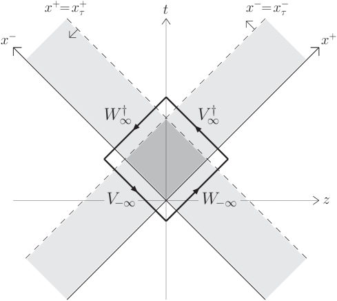
Figure 3: The distribution of the various background fields in the $x^{+}-x^{-}$ plane. The overlap region around the tip of the light–cone is the interaction region relevant for quantum evolution (see Sect. 5). The contour surrounding the interaction region will be explained in Sect. 7.

It should be clear by now that the result of resumming all splitting diagrams like Fig. 2.b is quadratic in $\rho$ and non–linear to all orders in $\delta A^{-}$, upon which it depends via the Wilson lines $W$ and $W^{\dagger}$. It is furthermore intuitively clear, and will be more formally justified in the next section, that the effects of such diagrams on the evolution of the $n$–point functions of the color charge $\rho$ can be obtained with the replacement

$$\delta\!A^{-}_{a}(x^{+},\bm{x})\to i\frac{\delta}{\delta\rho_{a}(x^{+},\bm{x})}\,.$$ (3.14)

We thus anticipate that the evolution Hamiltonian describing bremsstrahlung in the dilute regime should have the following general structure:

$$H_{\rm BREM}\,=\,\frac{1}{2}\,\rho\,\chi_{\rm BREM}[W,W^{\dagger}]\,\rho\,,\vspace{-.5cm}$$ (3.15)

where $\rho\equiv\rho_{a}(\bm{x})$ is integrated over $x^{-}$, so like in Eq. (3.10), since in this regime there is no multiple scattering in the $x^{-}$ direction. What is, however, more subtle now is the $x^{+}$–dependence of $\rho$, which was irrelevant in the BFKL and the JIMWLK approximations, but which becomes an issue in the presence of multiple scattering in the $x^{+}$ direction: With the prescription (3.14), the Wilson line (3.13) generates functional derivatives with respect to $\rho_{a}(x^{+},\bm{x})$ at all the points $x^{+}$ within the temporal extent $\Delta x^{+}$ of the fluctuating field $\delta A^{-}_{a}$. Thus, the Hamiltonian (3.15) acts naturally on a Hilbert space in which the color charge density carries also $x^{+}$ dependence. This shows that, in order to include correlations associated with gluon splitting, one needs a generalization of the original CGC effective theory which allows for time dependence. We shall see later that such a generalization can be indeed given, but it cannot account for the detailed temporal correlations that are a priori encoded in a Hamiltonian like (3.15). This is a consequence of the separation of scales in the problem: the semi–fast gluon has small $k^{-}$ relative to the background field $\delta\!A^{-}$, so it cannot resolve the structure of the latter in $x^{+}$, but measures only its overall distribution, via the temporal Wilson line $W$. This is similar, but dual — in the sense of exchanging $x^{-}$ by $x^{+}$, $\widetilde{A}^{+}$ by $\delta\!A^{-}$, and thus $V^{\dagger}$ by $W$ — to the JIMWLK problem, in which the semi–fast gluon is unable to discriminate the detailed $x^{-}$–structure of the fast sources, but measures them only via the longitudinal Wilson line $V^{\dagger}$. Inspired by this analogy, one can already anticipate that, when interpreted in the sense of RG, the BREM Hamiltonian (3.15) describes the evolution of the correlation functions for $W$ and $W^{\dagger}$, while the external factors of $\rho$ act as Lie derivatives on these Wilson lines. This is what we shall find indeed in the subsequent analysis.

The previous discussion suggests an interesting duality between the evolution in the dense and the dilute regimes, which in turn reflects a mirror symmetry between the $n\rightarrow 2$ and $2\rightarrow n$ vertices in Figs. 2. a and b, respectively. Specifically, the corresponding Hamiltonians should correspond to each other via the following duality transformation :

$$x^{-}\longleftrightarrow\,x^{+},\qquad\alpha^{a}(x^{-},\bm{x})\,\longleftrightarrow\,i\frac{\delta}{\delta\rho_{a}(x^{+},\bm{x})}\,,\qquad\frac{1}{i}\,\frac{\delta}{\delta\alpha^{a}(x^{-},\bm{x})}\,\longleftrightarrow\,\rho_{a}(x^{+},\bm{x})\,.\vspace{-.5cm}$$ (3.16)

Anticipated by earlier works on a symmetric formalism of the high–energy scattering problem in QCD [6, 7, 8, 10], such a duality has been recently found to hold in the large–$N_{c}$ approximation [35], where the only non–trivial vertices are the $1\rightarrow 2$ and $2\rightarrow 1$ triple–pomeron vertices, and the coordinates $x^{+}$ and $x^{-}$ play no dynamical role. Furthermore, Kovner and Lublinsky have argued [39] that the duality between mergings and splittings should hold exactly, i.e., beyond the large–$N_{c}$ approximation, as a consequence of a more general, self–duality, property of the general (unknown) evolution Hamiltonian.

However, the authors of Ref. [39] have mistaken $x^{+}$ for $x^{-}$ in the bremsstrahlung problem, and thus they failed to also recognize the $x^{-}\leftrightarrow x^{+}$ duality. But after correcting for this misidentification, we shall see that the self–duality idea is essentially right. The general evolution Hamiltonian that we shall construct in the next sections turns out to be invariant under a generalized duality transformation which exchanges Wilson lines in $x^{-}$ (so like $V^{\dagger}$) with those in $x^{+}$ (like $W$). Moreover, the expressions for $H_{\rm JIMWLK}$ and $H_{\rm BREM}$ that we shall find are indeed dual each other in the sense of Eq. (3.16). Our explicit construction will further clarify the origin and the physical meaning of this duality.

The general Hamiltonian alluded to above includes all the $m\to n$ processes for arbitrary integers $m\geq 2$ and $n\geq 2$ (see Fig. 2.c). To resum such processes one needs the propagator of the semi–fast gluon in the presence of both types of background field: the field $\widetilde{A}^{+}_{a}\equiv\alpha_{a}$ generated by the fast partons ($p^{+}\gg\Lambda$) and the field $\delta A^{-}_{a}$ associated with the soft quantum fluctuations ($k^{+}\sim b\Lambda$). This problem is complicated because the semi–fast gluons are at the same time slow relative to $\widetilde{A}^{+}_{a}$ and fast as compared to $\delta A^{-}_{a}$, so in general the eikonal approximation cannot be applied. However, for the purpose of RG, the propagator is needed only for points $x^{+}$ and $x^{-}$ near the origin of the light–cone, that is, in the region where the fields $\widetilde{A}^{+}_{a}$ and $\delta A^{-}_{a}$ overlap with each other (see Fig. 3). In this region, we shall be able to construct the propagator, and then the evolution Hamiltonian. The latter will be expressed in terms of Wilson lines (line–ordered phases in both $x^{-}$ and $x^{+}$) which run around the interaction region in Fig. 3 and represent the basic degrees of freedom. The general Hamiltonian turns out to be local in the transverse coordinates. The non–localities in the standard expressions for the JIMWLK [15, 11] and BREM [39] Hamiltonians (which here will be generated by expanding the general Hamiltonian in appropriate limits) are merely related to the non–locality of the relation (3.4) between the color field in the Coulomb gauge and its source.

4 Quantum evolution: The effective action

With this section, we start our explicit construction of the evolution Hamiltonian for QCD at high energy. This Hamiltonian must encompass processes like that in Fig. 2.c to all orders in the two types of background field : the ones above and those below the horizontal gluon line. The resummation of these diagrams can be formulated as a one–loop calculation in the quantum version of the effective theory for the CGC [14, 15]. This is a theory in which the fast partons with longitudinal momenta $p^{+}\gg\Lambda$ are represented by a random color charge density $\rho_{a}(x^{-},\bm{x})$ with weight function ${\cal W}_{\Lambda}[\rho]$ while the slow gluons with momenta $\leq\Lambda$ are still explicitly present as quantum fluctuations. Thus, this effective theory allows for the calculation of gluon correlations at any scale $k^{+}\leq\Lambda$.

For instance, the 2–point correlation function is obtained as:

$$\langle{\rm T}A^{\mu}(x)A^{\nu}(y)\rangle=\int D[\rho]\,{\cal W}_{\Lambda}[\rho]\,\frac{\int^{\Lambda}D\delta\!A\,A^{\mu}(x)A^{\nu}(y)\,\exp(iS[A,\rho])}{\int^{\Lambda}D\delta\!A\,\exp(iS[A,\rho])}$$ (4.1)

where the symbol T denotes time–ordering and it is understood that the two fields inside the brackets ‘live’ both at the same soft scale, i.e., $k^{+}_{1}\sim k^{+}_{2}\leq\Lambda$. Furthermore, the action $S[A,\rho]$ describes the gluon dynamics in the presence of the ‘external’ (or ‘background’) color source $\rho$, and the total field $A^{\mu}$ is the sum of the background field generated by $\rho$ and the quantum fluctuations $\delta\!A^{\mu}$ with momenta $p^{+}\leq\Lambda$. As we shall see, the background field itself is influenced by the fluctuations. The action $S[A,\rho]$ is such that it generates the classical field equations (3.1) in the limit where $\delta\!A^{\mu}=0$, but its precise form will not be needed below.

The one–step quantum evolution consists in integrating out the semi–fast fluctuations with momenta $\Lambda\gg|p^{+}|\gg b\Lambda$ where $b\ll 1$ but such that $\alpha_{s}\ln(1/b)\ll 1$. To that aim, we shall assume that the external fields in Eq. (4.1) carry momenta $k^{+}\sim b\Lambda$ and we shall compute the correlations induced at the soft scale $b\Lambda$ after integrating out the semi–fast fields $a^{\mu}$. That is, the total field within the action is now decomposed as

$$A^{\mu}=B^{\mu}+a^{\mu}+\delta\!A^{\mu},\vspace{-.5cm}$$ (4.2)

where $B^{\mu}$ is the background field generated by $\rho$, $a^{\mu}$ represents the semi–fast fluctuations, and $\delta\!A^{\mu}$ stands for the remaining fluctuations with $k^{+}\leq b\Lambda$. Note that the total field at the scale $b\Lambda$ (so like the external field in Eq. (4.1)) is simply $A^{\mu}=B^{\mu}+\delta\!A^{\mu}$.

After separating the soft from the semi–fast modes in the functional integral, the quantum average in Eq. (4.1) becomes:

$$\int^{b\Lambda}D\delta\!A\,A^{\mu}(x)A^{\nu}(y)\int_{b\Lambda}^{\Lambda}Da\exp(iS[A,\rho]),$$ (4.3)

where the last integration in Eq. (4.3) defines the effective action that we want to compute:

$$\exp(iS_{\rm eff})\equiv\int_{b\Lambda}^{\Lambda}Da\,\exp(iS[A,\rho]).$$ (4.4)

This is an action for the soft fields $\delta\!A^{\mu}$ which depends also upon $\rho$. From this action, the evolution Hamiltonian will be eventually obtained via the replacement (3.14) (or, rather, a generalization of it), that we shall shortly justify.

So far, we have not specified the gauge in which the quantum theory is defined. With the separation of scales in $k^{+}$ being not gauge–invariant, this issue is indeed important. The partonic interpretation of gluons is meaningful in the light–cone quantization which is defined in the LC–gauge $A^{+}=0$, so this is the gauge that we shall adopt in what follows. Note that the separation of scales in $k^{+}$ is invariant under the residual gauge transformations in the LC–gauge, which are independent of $x^{-}$. In fact, the separation of scales can be also formulated in a gauge–invariant way, as we shall later explain, but the use of the LC–gauge in the quantum calculation turns out to be really convenient. We should stress however that our calculation will be manifestly covariant with respect to the ‘background’ fields $B^{\mu}$ and $\delta\!A^{\mu}$, so the final result for the effective action will be gauge–invariant.

In the LC–gauge and for $\delta\!A^{\mu}=0$, the classical solution has only transverse components $A^{i}$ which are given by Eq. (3.5); these are time–independent and satisfy $F^{ij}=0$. But in order to compute diagrams like that in Fig. 2.c we need to preserve an explicit background field $\delta\!A^{-}$ (the component of the soft field $\delta\!A^{\mu}$ which couples to the semi–fast gluon), and this will also modify the classical field problem, by introducing time–dependence. Namely, in the presence of $\delta\!A^{-}$, the color source $\rho$ will be subjected to color precession :

$$\rho(\vec{x})\equiv\rho_{a}(\vec{x})T^{a}\ \longrightarrow\ J^{+}(x^{+},\vec{x})=W_{x^{+},-\infty}\,\rho(\vec{x})\,W_{x^{+},-\infty}^{\dagger}\,,\vspace{-.5cm}$$ (4.5)

meaning that the fast partons represented by $\rho$ undergo eikonal scattering off the field $\delta\!A^{-}$. In the equation above,

$$W_{x^{+},-\infty}(\bm{x})={\rm P}\exp\left\{{ig\int_{-\infty}^{x^{+}}{\rm d}z^{+}\delta\!A^{-}(z^{+},\bm{x})}\right\},$$ (4.6)

is the temporal Wilson line from $z^{+}\to-\infty$ up to the actual time $x^{+}$. Note that the current $J^{\mu}=\delta^{\mu+}J^{+}$ is covariantly conserved, as it should:

$$D_{\mu}J^{\mu}=D^{-}J^{+}=(\partial^{-}-ig\delta A^{-})J^{+}=0\,.\vspace{-.5cm}$$ (4.7)

We have anticipated here that $B^{-}=0$, so that $A^{-}=\delta A^{-}$ indeed. From Eq. (4.5), one sees that one can identify $\rho$ with the asymptotic value of the current $J^{+}$ at $x^{+}\to-\infty$, and in what follows it will be useful to write:

$$\rho_{-\infty}(\vec{x})\,\equiv\,J^{+}(x^{+}\to-\infty,\vec{x})=\rho(\vec{x}),\qquad\rho_{\infty}(\vec{x})\,\equiv\,J^{+}(x^{+}\to\infty,\vec{x}).\vspace{-.5cm}$$ (4.8)

The background field $B^{\mu}=\delta^{\mu i}B^{i}$ is defined as the solution to the Poisson equation with the current (4.5) :

$$\frac{\delta S}{\delta A^{-}}\Big{|}_{B^{i}+\delta\!A^{-}}=\,0\quad\Longrightarrow\quad D_{\nu}F^{\nu+}=J^{+}=W_{x^{+},-\infty}\rho_{-\infty}(\vec{x})W_{x^{+},-\infty}^{\dagger},$$ (4.9)

where, with a slight abuse of notations, the background field $A^{\mu}=\delta^{\mu i}B^{i}+\delta^{\mu-}\delta\!A^{-}$ has been denoted as $B^{i}+\delta\!A^{-}$.

A crucial observation for what follows is that

$$F^{-+}=-\partial^{+}\delta\!A^{-}\simeq 0,\vspace{-.5cm}$$ (4.10)

which follows from the fact that the field $\delta\!A^{-}$ contains only modes with very small longitudinal momenta and therefore it varies very slowly with $x^{-}$. More generally, the statement that $F^{-+}=0$ represents the gauge–invariant expression of the separation of scales in the problem. With this property, Eq. (4.9) simplifies to

$$D_{i}F^{i+}=-D_{i}\partial^{+}B^{i}=J^{+},$$ (4.11)

which will be shortly used to determine the field $B^{i}$ as a function of $\delta\!A^{-}$ and $\rho$. Notice the time dependence in the above equation : this is local in $x^{+}$, so $B^{i}$ and $J^{+}$ have the same time dependence, which in turn comes from the color precession in Eq. (4.5). Since the soft gauge field $\delta\!A^{-}$ has support at small $x^{+}$ (cf. Fig. 3), the temporal Wilson line (4.6) looks like a smooth $\Theta$–function in $x^{+}$ — its variation with $x^{+}$ is concentrated in a small region above $x^{+}=0$. A similar $x^{+}$–dependence then holds for both $J^{+}$ and $B^{i}$.

For the purpose of the one–loop calculation, the action $S$ must be expanded to second order in the semi–fast fields $a^{\mu}$. We obtain, with condensed notations,

$$S\,=\,S[B^{i}+\delta\!A^{\mu},\rho]+\,\frac{\delta S}{\delta A^{i}}\Big{|}_{B^{i}+\delta\!A^{-}}a^{i}+\,\frac{1}{2}\,a^{\mu}\,G_{\mu\nu}^{-1}[B^{i}+\delta\!A^{-},\rho]\,a^{\nu}\,,$$ (4.12)

where

$$\frac{\delta S}{\delta A^{i}}\Big{|}_{B^{i}+\delta\!A^{-}}=D_{\nu}F^{\nu i}=D_{j}F^{ji}+D_{-}F^{-i}+D_{+}F^{+i},$$ (4.13)

and

$$G_{\mu\nu}^{-1,\,ab}(x,y)\,[B^{i}+\delta\!A^{-},\rho]\,\equiv\,\frac{\delta^{2}S}{\delta A_{a}^{\mu}(x)\delta A_{b}^{\mu}(y)}\Big{|}_{B^{i}+\delta\!A^{-}}\,.\vspace{-.5cm}$$ (4.14)

As indicated in the equations above, only the $\delta\!A^{-}$ component of the soft field $\delta\!A^{\mu}$ needs to be kept in the terms describing the coupling with $a^{\mu}$.

Using again the fact that $\partial^{+}\delta\!A^{-}\simeq 0$, one can easily show that

$$D_{-}F^{-i}\simeq D_{+}F^{+i},$$ (4.15)

a relation which lies at the origin of the duality property, as we shall later see.

Consider now the Poisson equation (4.11) which determines $B^{i}$. As compared to the corresponding equation for $\delta\!A^{-}=0$ (the component $\mu=+$ of Eq. (3.1)), the present equation involves time dependence via $J^{+}$. However, this dependence is local, so the solution to Eq. (4.11) is again of the form $B^{i}=(i/g)U\partial^{i}U^{\dagger}$ (cf. Eq. (3.5)), except that now the Wilson lines depend also upon $x^{+}$ :

$$U^{\dagger}(x)={\rm P}\exp\left\{ig\int_{-\infty}^{x^{-}}{\rm d}z^{-}\alpha(x^{+},z^{-},\bm{x})\right\}.$$ (4.16)

Here, $\alpha\equiv\tilde{B}^{+}$ is the background field in the Coulomb gauge, defined by the time–dependent generalization of Eq. (3.3) :

$$-\nabla^{2}_{\perp}\alpha(x)\,=\,{\widetilde{\rho}}(x)\,\equiv\,U^{\dagger}(x)\,J^{+}(x)\,U(x)\,,\vspace{-.5cm}$$ (4.17)

which is local in both $x^{-}$ and $x^{+}$. The field $B^{i}$ constructed above is a two–dimensional pure gauge ($F^{ij}=0$), so Eq. (4.13) simplifies to

$$\frac{\delta S}{\delta A^{i}}\Big{|}_{B^{i}+\delta\!A^{-}}\simeq 2D_{+}F^{+i}\simeq 2D_{-}F^{-i}.$$ (4.18)

Performing the Gaussian integration over the semifast modes $a$ in Eq. (4.4), we finally arrive at the following expression for the effective action: $S_{\rm eff}=S+\Delta S_{\rm eff}$ with

$$\Delta S_{\rm eff}[\delta\!A^{-},\rho]\,=\,-\frac{1}{2}\int\limits_{xy}\,(2D^{-}F^{+i})_{x}^{a}\,G^{ij}_{ab}(x,y)\,(2D^{-}F^{+i})_{y}^{b}\,,$$ (4.19)

or, equivalently (within the present approximations),

$$\Delta S_{\rm eff}[\delta\!A^{-},\rho]\,=\,-\frac{1}{2}\int\limits_{xy}\,(2D^{+}F^{-i})_{x}^{a}\,G^{ij}_{ab}(x,y)\,(2D^{+}F^{-i})_{y}^{b}\,,$$ (4.20)

In these equations, $iG^{ij}$ are the transverse components of the time–ordered propagator of the semi–fast gluons:

$$iG^{\mu\nu}_{ab}(x,y)\,[B^{i}+\delta\!A^{-},\rho]\,\equiv\,\langle{\rm T}\,a^{\mu}_{a}(x)\,a^{\nu}_{b}(y)\rangle,\vspace{-.5cm}$$ (4.21)

where the brackets denote the average over the quantum fields $a^{\mu}$ for fixed values of the background fields $B^{i}$ and $\delta\!A^{-}$. This propagator can be obtained by inverting the differential operator in the r.h.s. of Eq. (4.14) in the LC gauge and with appropriate (Feynman) boundary conditions.

Eqs. (4.19) and (4.20) are the fundamental formulae which will allow us to construct the evolution Hamiltonian in the next sections. As anticipated, these expressions are manifestly invariant under the gauge transformations of the background fields (with the propagator $G^{ij}$ being covariant under such transformations). In what follows, we shall use this symmetry to replace the LC–gauge background fields $A^{\mu}=\delta^{\mu i}B^{i}+\delta^{\mu-}\delta\!A^{-}$ by the Coulomb gauge ones $\widetilde{A}^{\mu}=\delta^{\mu+}\alpha+\delta^{\mu-}\widetilde{\delta\!A}^{-}$, which are most directly related to the various Wilson lines. In the last equation, $\widetilde{\delta\!A}^{-}$ is the soft field in the Coulomb gauge:

$$\widetilde{\delta\!A}^{-}(x)=U^{\dagger}(x)\left[\delta\!A^{-}(x^{+},\bm{x})+\frac{i}{g}\partial^{-}\right]U(x),$$ (4.22)

and depends on $x^{-}$ (unlike its LC–gauge counterpart) via the corresponding dependence of the gauge rotation. That is, $\widetilde{\delta\!A}^{-}$ looks like a smooth $\Theta$–function in $x^{-}$. One can check on Eq. (4.22) that the condition $\widetilde{F}^{-+}=0$ (cf. Eq. (4.10)) remains satisfied, as it should.

In fact, with the background fields in the Coulomb gauge, one has:

$$\widetilde{D}^{+}=\partial^{+}-ig\alpha,\quad\widetilde{F}^{+i}=-\partial^{i}\alpha,\quad\widetilde{D}^{-}=\partial^{-}-ig\widetilde{\delta\!A}^{-},\quad\widetilde{F}^{-i}=-\partial^{i}\widetilde{\delta\!A}^{-}\,.\vspace{-.5cm}$$ (4.23)

We shall later argue that, under the present approximations, the transverse propagator

$$\widetilde{G}^{ij}_{ab}(x,y)[\,\alpha,\widetilde{\delta\!A}^{-}]\,=\,U^{\dagger}(x)\,\,G^{ij}_{ab}(x,y)\,[\,B^{i},\delta\!A^{-}]\,\,U(y)\,,\vspace{-.5cm}$$ (4.24)

is invariant under the exchange of plus and minus components for coordinates and fields:

$$x^{-}\longleftrightarrow\,x^{+},\qquad\alpha_{a}(x)\,\longleftrightarrow\,\widetilde{\delta\!A}^{-}_{a}(x).\vspace{-.5cm}$$ (4.25)

Therefore, under the transformations (4.25) the two expressions for the effective action, Eqs. (4.19) and (4.20), get interchanged. But since these expressions are equivalent with each other, we conclude that the effective action is invariant under the transformations (4.25). This symmetry is the most general form of the property that in the previous sections has been referred to as ‘self–duality’.

The physical meaning of this symmetry is easy to understand. The same one–loop calculation resumming the diagrams illustrated in Fig. 2.c can be interpreted in two ways: (i) As the evolution of the color fields $\widetilde{A}^{+}\equiv\alpha$ of the target with decreasing $k^{+}$ and in the presence of the fields $\widetilde{\delta\!A}^{-}$ of the projectile (this is the interpretation a priori privileged by our previous manipulations, and it corresponds to the expression (4.19) for the effective action), or (ii) as the evolution of the color fields $\widetilde{\delta\!A}^{-}$ of the projectile with decreasing $k^{-}$ and in the presence of the fields $\widetilde{A}^{+}\equiv\alpha$ of the target (this interpretation corresponds to Eq. (4.20) and amounts to reading a diagram like Fig. 2.c upside down). By virtue of boost invariance, the two directions of evolution must be equivalent: the rapidity increment $d\tau$ can be given to either the target or the projectile, with identical results for the evolution of the scattering amplitudes, which are Lorentz–invariant. This equivalence is indeed manifest at the level of our results, as the invariance of the effective action under the change (4.25) of the direction of evolution.

To conclude this section, let us justify the replacement (3.14) which will allow us to transform the effective action (a functional of $\rho$ and ${\delta\!A}^{-}$) into an evolution Hamiltonian involving $\rho$ and $\delta/\delta\rho$. This step is essential for promoting the above one–loop calculation into a systematic renormalization group (RG) procedure. The purpose of RG is to shift the newly induced correlations at the soft scale $b\Lambda$ from the effective action $\Delta S_{\rm eff}$ to the weight function ${\cal W}_{\tau}[\rho]$ for $\rho$. To that aim, it is preferable to work in the Coulomb background gauge, since scattering observables are directly related to $\widetilde{A}^{+}\equiv\alpha$, and not to $B^{i}$. Consider then the evolution

$$\langle{\rm T}\alpha(x)\alpha(y)\rangle_{b\Lambda}-\langle{\rm T}\alpha(x)\alpha(y)\rangle_{\Lambda}\vspace{-.5cm}$$ (4.26)

of the 2–point function when decreasing $k^{+}$ from $\Lambda$ to $b\Lambda$. We would like to associate this evolution with a change $\alpha\to\alpha+\delta\alpha$ in the classical field ; through Eq. (4.17), this corresponds to a change $\widetilde{\rho}\to\widetilde{\rho}+\delta\widetilde{\rho}$ in the charge density in the Coulomb gauge. Physically, $\delta\widetilde{\rho}$ represents the color charge density of the semi–fast gluons. To reproduce the correlations encoded into $\Delta S_{\rm eff}$, the induced source $\delta\widetilde{\rho}$ must be a random variable (for a fixed distribution $\widetilde{\rho}$ of the color charge at scale $\Lambda$), with correlations:

$$\langle{\rm T}\delta\widetilde{\rho}(x_{1})\delta\widetilde{\rho}(x_{2})\cdots\delta\widetilde{\rho}(x_{n})\rangle_{\widetilde{\rho}}\,=\,i^{n+1}\Gamma_{n}(x_{1},x_{2},\dots,x_{n})\,\equiv\,\frac{i^{n+1}\,\delta^{n}\Delta S_{\rm eff}}{\delta\widetilde{A}^{-}(x_{1})\delta\widetilde{A}^{-}(x_{2})...\delta\widetilde{A}^{-}(x_{n})}\Big{|}_{\widetilde{A}^{-}=0},$$

where for more clarity we have temporarily denoted $\widetilde{\delta\!A}^{-}$ simply as $\widetilde{A}^{-}$. Indeed, the quantum calculation yields (for the example of the 2–point function, once again)

$$\langle{\rm T}\,\widetilde{\delta\!A}^{+}\!(x)\,\widetilde{\delta\!A}^{+}\!(y)\rangle_{\widetilde{\rho}}=\int^{b\Lambda}D\widetilde{\delta\!A}\,\,\,\widetilde{\delta\!A}^{+}\!(x)\,\widetilde{\delta\!A}^{+}\!(y)\,\exp\big{\{}i\big{(}S[\,\widetilde{\delta\!A}\,]+\Delta S_{\rm eff}[\,\widetilde{\delta\!A}^{-},\widetilde{\rho}\,]\big{)}\big{\}},\vspace{-.5cm}$$ (4.28)

where the path–integral in the r.h.s. is now evaluated in the Coulomb gauge. To the accuracy of interest, this has to be computed in the saddle point approximation and to order $\alpha_{s}\ln(1/b)$ (recall that the induced action $\Delta S_{\rm eff}$ is itself of $\cal{O}(\alpha_{s}\ln(1/b))$). This yields:

$$\langle{\rm T}\,\widetilde{\delta\!A}^{+}\!(x)\,\widetilde{\delta\!A}^{+}\!(y)\rangle_{\widetilde{\rho}}\,\simeq\,i\int\limits_{u,v}iG^{+-}(x,u)\,iG^{+-}(y,v)\,\,\Gamma_{2}(u,v)\,,\vspace{-.5cm}$$ (4.29)

which should be compared to the corresponding correlation induced, via the classical field equation (4.17), by a change $\delta\widetilde{\rho}$ in the color source:

$$\langle{\rm T}\delta\alpha(x)\delta\alpha(y)\rangle_{\widetilde{\rho}}\,=\,\int\limits_{u,v}\Delta(x-u)\Delta(y-v)\,\,\langle{\rm T}\,\delta\widetilde{\rho}(u)\,\delta\widetilde{\rho}(v)\rangle_{\widetilde{\rho}}\,.\vspace{-.5cm}$$ (4.30)

In the static limit $p^{-}=0$, $G^{+-}(x,u)=\Delta(x-u)$, and the above correlations coincide with each other provided Eq. (4) is satisfied.

Finally, it is clear that the Hamiltonian which, when acting on correlations of $\widetilde{\rho}$ (cf. Eq. (3.8)), generates the correlations in Eq. (4) is of the form (with ${\rm d}\tau=\ln 1/b$) :

$$-{\rm d}\tau\,H\Big{[}\widetilde{\rho},\,i\frac{\delta}{\delta\widetilde{\rho}}\Big{]} \,=\, \sum_{n}\frac{1}{n!}\,\int\limits_{x_{i}}\,\Gamma_{n}(x_{1},x_{2},\dots,x_{n})\,\frac{i^{n+1}\,\delta^{n}}{\delta\widetilde{\rho}(x_{1})\delta\widetilde{\rho}(x_{2})...\delta\widetilde{\rho}(x_{n})}$$ (4.31)

$$\,=\, i\Delta S_{\rm eff}\Big{[}\,\widetilde{\rho},\,\,\widetilde{\delta\!A}^{-}\!=\,i\frac{\delta}{\delta\widetilde{\rho}}\,\Big{]}\,.\vspace{-.5cm}$$

Thus, the evolution Hamiltonian is obtained from the effective action via the replacement

$$\widetilde{\delta\!A}^{-}(x)\ \longrightarrow\ {i}\,\frac{\delta}{\delta\widetilde{\rho}(x)},$$ (4.32)

which generalizes the previous prescription (3.14) by including the dependence upon $x^{-}$ and by specifying that in the general, strong field, regime, this replacement works at the level of Coulomb gauge quantities.

5 The background field propagator

In this section we shall construct the background field propagator which is needed to compute the expressions (4.19) or (4.20) for the effective action. This is the propagator $G^{ij}(x,y)$ for a semi–fast, transverse, gluon in the quantum LC–gauge ($a^{+}=0$) and in the presence of a background field which can be taken either in the LC–gauge ($A^{\mu}=\delta^{\mu i}B^{i}+\delta^{\mu-}\delta\!A^{-}$), or in the Coulomb gauge ($\widetilde{A}^{\mu}=\delta^{\mu+}\alpha+\delta^{\mu-}\widetilde{\delta\!A}^{-}$), and which involves two independent field degrees of freedom. The general expression of this propagator is complicated and we shall not attempt to derive it here. But for the present purposes, a crucial simplification comes from the fact that Eqs. (4.19)–(4.20) involve the propagator $G^{ij}(x,y)$ only at points $x$ and $y$ within the interaction region in Fig. 3. By the ‘interaction region’ we mean the diamond–shape area around the tip of the light–cone where the supports of $\rho$ and $\delta\!A^{-}$ (or, equivalently, of $\alpha$ and $\widetilde{\delta\!A}^{-}$) overlap with each other. The essential property of this region is that its extent both in longitudinal and in temporal directions is very small as compared to the respective resolution scales of the semi–fast gluon. Because of that, the propagator $G^{ij}(x,y)$ is local in the transverse coordinates and has a relatively simple structure in the other coordinates, as we shall explain below.

Let us first establish the support properties of the integrands in Eqs. (4.19) or (4.20). Consider Eq. (4.19), for definiteness, and look at the vertices there: the field $F^{+i}$ has the same support as the color source $\rho$ at scale $\Lambda$, so it is localized in $x^{-}$ within the region $0\mathrel{\hbox to0.0pt{\raise 2.20013pt\hbox{$<$}\hss}{\lower 2.20013pt\hbox{$\sim$}}}x^{-}\mathrel{\hbox to0.0pt{\raise 2.20013pt\hbox{$<$}\hss}{\lower 2.20013pt\hbox{$\sim$}}}1/\Lambda$. Furthermore, its (covariant) derivative $D^{-}F^{+i}=(\partial^{-}-ig\delta\!A^{-})F^{+i}$ involves two terms, which are both localized at small $x^{+}$, within the support of $\delta\!A^{-}$. This is obvious for the second term, which is explicitly proportional to $\delta\!A^{-}$, but it is also true for the first term $\partial^{-}F^{+i}$, since the time–dependence of $F^{+i}$ comes entirely from its interaction with $\delta\!A^{-}$, as discussed after Eq. (4.11). Recalling that $\delta\!A^{-}$ has small $k^{+}\mathrel{\hbox to0.0pt{\raise 2.20013pt\hbox{$<$}\hss}{\lower 2.20013pt\hbox{$\sim$}}}b\Lambda$ and thus large $k^{-}\mathrel{\hbox to0.0pt{\raise 2.20013pt\hbox{$>$}\hss}{\lower 2.20013pt\hbox{$\sim$}}}Q^{2}/2b\Lambda$ (with $Q^{2}$ a typical transverse momentum scale), we deduce that $D^{-}F^{+i}$ has support at $0\mathrel{\hbox to0.0pt{\raise 2.20013pt\hbox{$<$}\hss}{\lower 2.20013pt\hbox{$\sim$}}}x^{+}\mathrel{\hbox to0.0pt{\raise 2.20013pt\hbox{$<$}\hss}{\lower 2.20013pt\hbox{$\sim$}}}b\Lambda/Q^{2}$. To summarize:

$$D^{-}F^{+i}\neq 0\qquad{\rm for}\quad 0\mathrel{\hbox to0.0pt{\raise 2.20013pt\hbox{$<$}\hss}{\lower 2.20013pt\hbox{$\sim$}}}x^{-}\mathrel{\hbox to0.0pt{\raise 2.20013pt\hbox{$<$}\hss}{\lower 2.20013pt\hbox{$\sim$}}}1/\Lambda\quad{\rm and}\quad 0\mathrel{\hbox to0.0pt{\raise 2.20013pt\hbox{$<$}\hss}{\lower 2.20013pt\hbox{$\sim$}}}x^{+}\mathrel{\hbox to0.0pt{\raise 2.20013pt\hbox{$<$}\hss}{\lower 2.20013pt\hbox{$\sim$}}}b\Lambda/Q^{2}.\vspace{-.5cm}$$ (5.1)

This is also the support of the vertex $D^{+}F^{-i}$ in Eq. (4.20). On the other hand, the semi–fast gluon has $\Lambda\gg k^{+}\gg b\Lambda$, and thus typical resolution scales $\Delta x^{-}\sim 1/b\Lambda$ and $\Delta x^{+}\sim\Lambda/Q^{2}$. Since, by assumption, $b\ll 1$, we conclude that the semi–fast gluon cannot discriminate the internal structure of the interaction region in Fig. 3, as anticipated.

This feature drastically simplifies the calculation of the semi–fast propagator. To better appreciate that, let us analyze first the corresponding free propagator :

$$G_{0}^{ij}(p)=\delta^{ij}G_{0}(p),\quad G_{0}^{i-}(p)=\frac{p^{i}}{p^{+}+i\epsilon}\,G_{0}(p),\quad G_{0}^{-i}(p)=\frac{p^{i}}{p^{+}-i\epsilon}\,G_{0}(p)\,,\vspace{-.5cm}$$ (5.2)

where $G_{0}(p)=1/(2p^{+}p^{-}-\bm{p}^{2}+i\epsilon)$ is the same as the propagator of a free scalar field. Consider the scalar propagator, and perform the Fourier transform to coordinate space:

$$G_{0}(x-y) = -i\int\limits_{\rm strip}\frac{dp^{+}}{2\pi}\,{\rm e}^{\frac{-ip^{+}(x^{-}-y^{-})}{2p^{+}}}\,\big{[}\Theta(p^{+})\Theta(x^{+}-y^{+})-\Theta(-p^{+})\Theta(y^{+}-x^{+})\big{]}$$ (5.3)

$$\qquad\qquad\times\ \int\frac{d^{2}\bm{p}}{(2\pi)^{2}}\,\,{\rm e}^{i\bm{p}\cdot(\bm{x}-\bm{y})-i\frac{\bm{p}^{2}}{2p^{+}}(x^{+}-y^{+})}\,,\,\,\vspace{-.5cm}$$

where the integration over $p^{-}$ has been computed via contour techniques and the integration over $p^{+}$ is restricted to the strip $\Lambda\gg|p^{+}|\gg b\Lambda$. The interesting region is where both $x^{-}-y^{-}$ and $x^{+}-y^{+}$ are small compared to the typical variation scales, $1/p^{+}$ and $1/p^{-}={2p^{+}}/{\bm{p}^{2}}$, respectively. Then we can neglect the longitudinal and temporal coordinates within the exponentials and perform the remaining integrations, to obtain:

$$iG_{0}^{ij}(x-y)\simeq\delta^{ij}\,\,\frac{1}{4\pi}\ln\frac{1}{b}\,\,\delta^{(2)}(\bm{x}-\bm{y}),\vspace{-.5cm}$$ (5.4)

where the logarithm has been generated by the restricted integration over $p^{+}$ :

$$\int\limits_{\rm strip}{\frac{dp^{+}}{2\pi}}\,\frac{\Theta(p^{+})}{2p^{+}}\,=\,-\int\limits_{\rm strip}\frac{dp^{+}}{2\pi}\,\frac{\Theta(-p^{+})}{2p^{+}}=\frac{1}{4\pi}\,\ln\frac{1}{b}\,.\vspace{-.5cm}$$ (5.5)

The final result, Eq. (5.4), is the same as the Fourier transform of the simplified momentum–space propagator in which $\bm{p}^{2}$ is neglected compared to $p^{+}p^{-}$ :

$$G_{0}(x-y)\simeq\int\limits_{\rm strip}\frac{dp^{+}}{2\pi}\,\int\frac{dp^{-}}{2\pi}\,\frac{1}{2p^{+}p^{-}+i\epsilon}\int\frac{d^{2}\bm{p}}{(2\pi)^{2}}\,\,{\rm e}^{i\bm{p}\cdot(\bm{x}-\bm{y})}\,.\vspace{-.5cm}$$ (5.6)

This is intuitive since small values for $x^{+}$ and $x^{-}$ correspond in momentum space to large values for $p^{-}$ and $p^{+}$, respectively. Similar approximations can be performed also in the presence of the background fields.

Consider first the case where there is only one such a field, namely $\delta\!A^{-}$. In the LC–gauge $a^{+}=0$, insertions of $\delta\!A^{-}$ cannot couple the transverse components $G^{ij}$ to any other component like $G^{i-}$; thus, the calculation of $G^{ij}\,[\delta\!A^{-}]$ is tantamount to that of the respective scalar propagator. The general expression for $G^{ij}(x,y)[\delta\!A^{-}]$ valid for arbitrary points $x$ and $y$ can be inferred from previous results in the literature (see, e.g., Ref. [15]). Here, however, we only need its expression valid within the interaction region, and this can be easily computed by solving the following differential equation

$$2\partial^{+}_{x}\big{[}\partial^{-}_{x}-ig\delta\!A^{-}(x)\big{]}G(x,y)=\delta^{(4)}(x-y),\vspace{-.5cm}$$ (5.7)

which has been obtained from the general Dyson equation after neglecting the transverse Laplacian $\nabla_{\perp}^{2}$ relative to $\partial^{+}D^{-}$, so like in Eq. (5.6). Working in the $p^{+}$ representation (since $\delta\!A^{-}$ is independent of $x^{-}$) and using $D^{-}_{x}W_{x^{+}y^{+}}(\bm{x})=0$ for $x^{+}>y^{+}$, where

$$W_{x^{+}y^{+}}(\bm{x})\equiv{\rm P}\exp\left\{{ig\int_{y^{+}}^{x^{+}}{\rm d}z^{+}\delta\!A^{-}(z^{+},\bm{x})}\right\},$$ (5.8)

one immediately finds that the solution to (5.7) with Feynman boundary conditions reads

$$iG^{ij}(x^{+},\bm{x},y^{+},\bm{y},p^{+})[\delta\!A^{-}]=\delta^{ij}\,\frac{1}{2p^{+}}\,\delta^{(2)}(\bm{x}-\bm{y})\big{[} \Theta(p^{+})\Theta(x^{+}-y^{+})W_{x^{+}y^{+}}(\bm{x})$$

$$-\Theta(-p^{+})\Theta(y^{+}-x^{+})W_{y^{+}x^{+}}^{\dagger}(\bm{x})\big{]}.$$ (5.9)

After also performing the restricted integration over $p^{+}$, one finally obtains :

$$iG^{ij}(x^{+},\bm{x},y^{+},\bm{y})[\delta\!A^{-}]=\delta^{ij}\,\frac{1}{4\pi}\ln\frac{1}{b}\,\,\delta^{(2)}(\bm{x}-\bm{y})\big{[} \Theta(x^{+}-y^{+})W_{x^{+}y^{+}}(\bm{x})$$

$$+\Theta(y^{+}-x^{+})W_{y^{+}x^{+}}^{\dagger}(\bm{x})\big{]}.$$ (5.10)

Consider similarly the case where the only background field is the one created by $\rho$, which is independent of $x^{+}$. If the field is taken in the Coulomb gauge, where it has just a plus component $\tilde{B}^{+}\equiv\alpha$, then the corresponding propagator is obtained by simply replacing $x^{+}\to x^{-}$ and $\delta\!A^{-}\to\alpha$ (and therefore $W_{x^{+}y^{+}}(\bm{x})\to U^{\dagger}_{x^{-}y^{-}}(\bm{x})$) in Eq. (5):

$$i\widetilde{G}^{ij}(x^{-},\bm{x},y^{-},\bm{y})[\alpha]=\delta^{ij}\,\frac{1}{4\pi}\ln\frac{1}{b}\,\,\delta^{(2)}(\bm{x}-\bm{y})\big{[} \Theta(x^{-}-y^{-})U^{\dagger}_{x^{-}y^{-}}(\bm{x})$$

$$+\Theta(y^{-}-x^{-})U_{y^{-}x^{-}}(\bm{x})\big{]}.$$ (5.11)

Note that, a priori, the insertions of $\alpha$ can couple the transverse semi–fast gluons $a^{i}$ to the temporal ones $a^{-}$, so in general the propagator $\widetilde{G}^{ij}[\alpha]$ will involve a mixture of all the components of the free propagator shown in Eq. (5.2). Still, for small $x^{-}$ and $y^{-}$ (within the interaction region) the coupling between transverse and temporal components is negligible since the off–diagonal propagators like $G^{i-}_{0}$ are suppressed when $p^{+}\gg p^{i}$.

If one now rotates the propagator (5) to the background LC–gauge, $\widetilde{G}^{ij}[\alpha]\to{G}^{ij}[B^{i}]$ with ${G}^{ij}(x,y)=U(x)\widetilde{G}^{ij}(x,y)U^{\dagger}(y)$, cf. Eq. (4.24), then one discovers that within the present approximations ${G}^{ij}[B^{i}]$ is the same as the free propagator (5.4) ! This can be easily understood: Unlike the Coulomb gauge field $\alpha$ which is singular at $x^{-}=0$ (on the resolution scale of the semi–fast gluons), the LC–gauge field $B^{i}$ is only discontinuous there, so the corresponding propagator ${G}^{ij}[B^{i}]$ must be continuous at both $x^{-}=0$ and $y^{-}=0$. Thus, for small separations $x^{-}-y^{-}\simeq 0$, the propagator will be independent of $x^{-}$ and $y^{-}$, and therefore also independent of the field $B^{i}$.

Armed with this experience from the simpler cases, we now turn to the general situation where both types of background field are simultaneously present. We shall first take these fields in the (background) LC–gauge, where $A^{\mu}=\delta^{\mu i}B^{i}+\delta^{\mu-}\delta\!A^{-}$. Then the propagator ${G}^{ij}[B^{i},\delta\!A^{-}]$ will be continuous at small $x^{-}$ (and thus independent of $B^{i}$), but discontinuous at small $x^{+}$ (and thus dependent upon $\delta\!A^{-}$ via the corresponding Wilson line (5.8)). We conclude that the general propagator that we need for the present purposes is the same as the propagator (5) in the presence of $\delta\!A^{-}$ alone. This is the propagator that we shall use for our most general calculations below.

But it is still interesting (in particular, for the self–duality argument in Sect. 4) to also consider the general propagator in the background Coulomb gauge, where $\widetilde{A}^{\mu}=\delta^{\mu+}\alpha+\delta^{\mu-}\widetilde{\delta\!A}^{-}$. This is obtained from Eq. (5) via the gauge–rotation (4.24), and it is found to involve products of temporal and longitudinal Wilson lines, of the type:

$$\widetilde{W}_{x^{+}y^{+}}(x^{-},\bm{x})U^{\dagger}_{x^{-}y^{-}}(y^{+},\bm{x})\,=\,U^{\dagger}_{x^{-}y^{-}}(x^{+},\bm{x})\widetilde{W}_{x^{+}y^{+}}(y^{-},\bm{x}),\vspace{-.5cm}$$ (5.12)

where $\widetilde{W}_{x^{+}y^{+}}$ is the temporal Wilson line in the Coulomb gauge:

$$\widetilde{W}_{x^{+}y^{+}}(x^{-},\bm{x}) \equiv U^{\dagger}(x^{-},x^{+},\bm{x})\,{W}_{x^{+}y^{+}}(\bm{x})\,U(x^{-},y^{+},\bm{x})\,$$ (5.13)

$$= {\rm P}\exp\left\{ig\int_{y^{+}}^{x^{+}}{\rm d}z^{+}\,\widetilde{\delta\!A}^{-}(z^{+},x^{-},\bm{x})\right\},\vspace{-.5cm}$$

with $\widetilde{\delta\!A}^{-}$ the corresponding field, cf. Eq. (4.22). The equality in Eq. (5.12) follows because, in the LC–gauge, ${W}_{x^{+}y^{+}}$ is independent of $x^{-}$, by Eq. (4.10). Note that Eq. (5.12) involves two possible paths joining the points $(x^{-},x^{+})$ and $(y^{-},y^{+})$; both these paths give the same contribution because of the condition $F^{+-}=0$, which reflects the separation of scales in the problem. But by the same condition, any other path joining these points will give an identical contribution, so the expressions in Eq. (5.12) can be equivalently replaced by

$${\rm P}\exp\left\{ig\int_{\gamma}\big{(}{\rm d}z^{+}\,\widetilde{\delta\!A}^{-}+{\rm d}z^{-}\alpha\big{)}(z^{+},z^{-},\bm{x})\right\},\vspace{-.5cm}$$ (5.14)

where the path $\gamma$ going from $(y^{-},y^{+})$ to $(x^{-},x^{+})$ must lie inside the interaction region, but otherwise is arbitrary. With the Wilson line (5.14), the Coulomb gauge propagator $\widetilde{G}^{ij}[\alpha,\widetilde{\delta\!A}^{-}]$ is clearly invariant under the transformations (4.25), as anticipated in Sect. 4.

6 The high density regime: JIMWLK Hamiltonian

Before we address the general case in the next section, it is instructive to see how the formalism works in a case for which the final result is already known: the strong field/no gluon number fluctuation regime, where the RG evolution is governed by the JIMWLK Hamiltonian [14, 15, 11]. For more variety in the presentation, the path that we shall follow in this section to recover the JIMWLK Hamiltonian will be different from that to be used in the next section in relation with the general case.

As it should be clear from a comparison between the diagrams in Figs. 2.a and c, and also from the general discussion in Sect. 3, the effective action corresponding to this regime is obtained by retaining terms to quadratic order in $\delta\!A^{-}$ and to all orders in $B^{i}$ (or $\alpha$) in the general expressions (4.19) and (4.20). Since the vertices $D^{-}F^{+i}$ or $D^{+}F^{-i}$ in these expressions start already at linear order in $\delta\!A^{-}$, it will be enough for the present purposes to consider the expression of the transverse propagator for $\delta\!A^{-}=0$. It turns out that the JIMWLK Hamiltonian is most efficiently obtained starting with Eq. (4.20) and working in the background Coulomb gauge. That is, we shall start with

$$\Delta S_{\rm eff}=-\frac{1}{2}\int\limits_{xy}(2\widetilde{D}^{+}\widetilde{F}^{-i})_{x}\widetilde{G}^{ij}(x,y)(2\widetilde{D}^{+}\widetilde{F}^{-i})_{y},$$ (6.1)

where $\widetilde{D}^{+}=\partial^{+}-ig\alpha$, $\widetilde{F}^{-i}=-\partial^{i}\widetilde{\delta\!A}^{-}$, and the propagator $\widetilde{G}^{ij}$ is given by Eq. (5).

The first step is to integrate by parts over the longitudinal coordinates $x^{-}$ and $y^{-}$. From Eq. (5), one can easily check that $\widetilde{D}^{+}_{x}\widetilde{G}^{ij}(x,y)=0$. By using this, together with the identity ($A$ and $B$ are two generic color matrices)

$$\partial^{\mu}(AB)=(D^{\mu}A)B+A(D^{\mu}B).$$ (6.2)

one can immediately deduce that the integrand in Eq. (6.1) is a total derivative w.r.t. both $x^{-}$ and $y^{-}$, so the result of the integration comes from the ‘surface’ terms at large (positive or negative) longitudinal coordinates. Specifically,

$$\Delta S_{\rm eff}=\frac{i}{2\pi} \,\ln\frac{1}{b}\int\limits_{x^{+},y^{+},\bm{x}}\big{[}\widetilde{F}^{-i}_{x^{+}}(\infty,\bm{x})\widetilde{F}^{-i}_{y^{+}}(\infty,\bm{x})+\widetilde{F}^{-i}_{x^{+}}(-\infty,\bm{x})\widetilde{F}^{-i}_{y^{+}}(-\infty,\bm{x})$$

$$-\widetilde{F}^{-i}_{x^{+}}(\infty,\bm{x})V^{\dagger}(\bm{x})\widetilde{F}^{-i}_{y^{+}}(-\infty,\bm{x})-\widetilde{F}^{-i}_{x^{+}}(-\infty,\bm{x})V(\bm{x})\widetilde{F}^{-i}_{y^{+}}(\infty,\bm{x})\big{]},$$ (6.3)

where (cf. Eq. (3.11)) :

$$V^{\dagger}({\bm{x}})=\,{\rm P}\,{\rm exp}\left\{ig\int{\rm d}x^{-}\alpha^{a}(x^{-},\bm{x})T^{a}\right\}\,.\vspace{-.5cm}$$ (6.4)

Note that the time arguments of the fields in Eq. (6) are shown as lower subscripts, a convention that we shall often use in what follows. As explained in Sect. 4, the difference between the fields $\widetilde{F}^{-i}(x^{-}=\infty)$ and $\widetilde{F}^{-i}(x^{-}=-\infty)$ comes from the interaction with the color source $\rho$, as encoded in the gauge rotations in Eq. (4.22). This interaction is localized at small $x^{-}$, so $\widetilde{F}^{-i}(x^{-})$ looks like a smooth $\Theta$–function in $x^{-}$.

By using $\widetilde{F}^{-i}=-\partial^{i}\widetilde{\delta\!A}^{-}$ and defining $\widetilde{A}^{-}(\vec{x})=\int{\rm d}x^{+}\,\widetilde{\delta\!A}^{-}(x)$, we obtain

$$\Delta S_{\rm eff}=\frac{i}{2\pi} \,\ln\frac{1}{b}\int\limits_{\bm{x}}\big{[}\partial^{i}\widetilde{A}^{-}(\infty,\bm{x})\partial^{i}\widetilde{A}^{-}(\infty,\bm{x})+\partial^{i}\widetilde{A}^{-}(-\infty,\bm{x})\partial^{i}\widetilde{A}^{-}(-\infty,\bm{x})$$

$$-\partial^{i}\widetilde{A}^{-}(\infty,\bm{x})V^{\dagger}(\bm{x})\partial^{i}\widetilde{A}^{-}(-\infty,\bm{x})-\partial^{i}\widetilde{A}^{-}(-\infty,\bm{x})V(\bm{x})\partial^{i}\widetilde{A}^{-}(\infty,\bm{x})\big{]}.$$ (6.5)

The evolution Hamiltonian can be now obtained via the replacement (4.32) (in four–dimensional coordinates !). By also using the Poisson equation (4.17) to reexpress ${\delta}/{\delta\widetilde{\rho}}$ in terms of ${\delta}/{\delta\alpha}$, we finally arrive at

$$H_{\rm JIMWLK}= \frac{-1}{(2\pi)^{3}}\,\int\limits_{\bm{x}\bm{y}\bm{z}}\mathcal{K}_{\bm{x}\bm{y}\bm{z}}\,\bigg{[}\frac{\delta}{\delta\alpha^{a}(\infty,\bm{x})}\frac{\delta}{\delta\alpha^{a}(\infty,\bm{y})}+\frac{\delta}{\delta\alpha^{a}(-\infty,\bm{x})}\frac{\delta}{\delta\alpha^{a}(-\infty,\bm{y})}$$

$$-\frac{\delta}{\delta\alpha^{a}(\infty,\bm{x})}V_{ab}^{\dagger}(\bm{z})\frac{\delta}{\delta\alpha^{b}(-\infty,\bm{y})}-\frac{\delta}{\delta\alpha^{a}(-\infty,\bm{x})}V_{ab}(\bm{z})\frac{\delta}{\delta\alpha^{b}(\infty,\bm{y})}\bigg{]},$$ (6.6)

with the following transverse kernel:

$${\mathcal{K}}({\bm{x},\bm{y},\bm{z}})\,\equiv\,\frac{(\bm{x}-\bm{z})\cdot(\bm{y}-\bm{z})}{(\bm{x}-\bm{z})^{2}(\bm{z}-\bm{y})^{2}}\,.\vspace{-.5cm}$$ (6.7)

In writing Eq. (6) we have suppressed the $x^{+}$ dependence although, strictly speaking, the integrand does depend upon time, via the functional derivatives which should be interpreted as, e.g.,

$$\frac{\delta}{\delta\alpha^{a}(\infty,\bm{x})}\,\equiv\,\int{\rm d}x^{+}\,\frac{\delta}{\delta\alpha^{a}(x^{+},\infty,\bm{x})}\,.\vspace{-.5cm}$$ (6.8)

But this dependence is rather trivial since when the Hamiltonian acts on scattering observables, like Eq. (2.1), the only contribution arises from the interaction time $x^{+}\simeq 0$.

On the other hand, the $x^{-}$ dependence of the Hamiltonian (6) is less trivial and deserves some comments: As mentioned before, $\widetilde{\delta\!A}^{-}(x)$ looks like a smooth $\Theta$–function in $x^{-}$, which varies within the range $0\mathrel{\hbox to0.0pt{\raise 2.20013pt\hbox{$<$}\hss}{\lower 2.20013pt\hbox{$\sim$}}}x^{-}\mathrel{\hbox to0.0pt{\raise 2.20013pt\hbox{$<$}\hss}{\lower 2.20013pt\hbox{$\sim$}}}x^{-}_{\tau}$, with $x^{-}_{\tau}\sim 1/\Lambda=(1/P^{+}){\rm e}^{\tau}$. Therefore, in the identification (4.32), the asymptotic fields $\widetilde{\delta\!A}^{-}(x^{-}\to\pm\infty)$ should be really understood as the values of the field at the end points $x^{-}_{0}\simeq 0$ and $x^{-}_{\tau}$ of this finite interval. Thus, strictly speaking,

$$\frac{\delta}{\delta\alpha^{a}(\infty,\bm{x})}\,\equiv\,\frac{\delta}{\delta\alpha^{a}_{\tau}(\bm{x})}\qquad{\rm and}\qquad\frac{\delta}{\delta\alpha^{a}(-\infty,\bm{x})}\,\equiv\,\frac{\delta}{\delta\alpha^{a}_{0}(\bm{x})},\vspace{-.5cm}$$ (6.9)

act as derivatives at the end points of the Wilson line in Eq. (3.11):

$$\frac{\delta V^{\dagger}({\bm{x}})}{\delta\alpha_{\tau}^{a}(\bm{y})}=ig\delta^{(2)}(\bm{x}-\bm{y})T^{a}V^{\dagger}({\bm{x}})\,,\qquad\frac{\delta V^{\dagger}({\bm{x}})}{\delta\alpha_{0}^{a}(\bm{y})}=ig\delta^{(2)}(\bm{x}-\bm{y})V^{\dagger}({\bm{x}})T^{a}.\vspace{-.5cm}$$ (6.10)

By comparing these results and using the identity $V_{ab}^{\dagger}T^{b}=VT^{a}V^{\dagger}$, one can express the derivatives at $x^{-}_{0}$ in terms of those at $x^{-}_{\tau}$:

$$\frac{\delta}{\delta\alpha^{a}_{0}(\bm{x})}\,=\,\frac{\delta}{\delta\alpha^{b}_{\tau}(\bm{x})}\,V_{ba}^{\dagger}(\bm{x})\,=\,V_{ab}(\bm{x})\,\frac{\delta}{\delta\alpha^{b}_{\tau}(\bm{x})}\,.$$ (6.11)

Alternatively, and more generally, Eq. (6.11) can be obtained as the result of a gauge rotation, as we show now. Let us first introduce the gauge–covariant ‘color current’ :

$$J^{-}(x)\equiv D_{\nu}F^{\nu-}(x)=D_{i}F^{i-}+D_{+}F^{+-}=D^{i}F^{-i},\vspace{-.5cm}$$ (6.12)

where in writing the last equality we have used $F^{+-}=0$, cf. Eq. (4.10). (In a scattering problem, in which $\delta A^{-}$ would be the field created by a left–moving projectile, $J^{-}_{a}$ would be the color current associated with the latter.) Under the gauge rotation (4.16) from the LC– to the Coulomb gauge, this current transforms like:

$$\widetilde{J}^{-}(x)\,\,=\,U^{\dagger}(x)\,J^{-}(x)\,U(x)\,,\vspace{-.5cm}$$ (6.13)

a relation which for $x^{-}=\infty$ can be rewritten as:

$$\widetilde{J}^{-}_{a}(x^{+},\infty,\bm{x})\,=\,U^{\dagger}_{ab}(x^{+},\infty,\bm{x})\,\widetilde{J}^{-}_{a}(x^{+},-\infty,\bm{x})\,.\vspace{-.5cm}$$ (6.14)

By also using $\widetilde{F}^{-i}=-\partial^{i}\widetilde{\delta\!A}^{-}$ together with Eqs. (6.12), (4.32) and (4.17), one can successively write

$$\widetilde{J}^{-}_{a}(x)\,=\,-\nabla^{2}_{\perp}\widetilde{\delta\!A}^{-}_{a}(x)\ \longrightarrow\ -\nabla^{2}_{\perp}\,\frac{{i}\,\delta}{\delta\widetilde{\rho}_{a}(x)}\,=\,i\,\frac{\delta}{\delta\alpha_{a}(x)}\,.\vspace{-.5cm}$$ (6.15)

By inserting this representation for $\widetilde{J}^{-}_{a}(x)$ in both the l.h.s. and the r.h.s. of Eq. (6.14), and recalling that $U^{\dagger}(x^{+},\infty,\bm{x})\approx V^{\dagger}(\bm{x})$ in the present regime (small ${\delta\!A}^{-}$), we finally recover the relation (6.11), as anticipated.

After using Eqs. (6.9) and Eq. (6.11), the JIMWLK Hamiltonian (6) takes its standard form:

$$H_{\rm JIMWLK}= \frac{-1}{(2\pi)^{3}}\,\int\limits_{\bm{x}\bm{y}\bm{z}}\mathcal{K}_{\bm{x}\bm{y}\bm{z}}\,\frac{\delta}{\delta\alpha^{a}_{\tau}(\bm{x})}\Big{[}1+V^{\dagger}_{\bm{x}}V_{\bm{y}}-V^{\dagger}_{\bm{z}}V_{\bm{y}}-V^{\dagger}_{\bm{x}}V_{\bm{z}}\Big{]}^{ab}\frac{\delta}{\delta\alpha^{b}_{\tau}(\bm{y})},$$ (6.16)

as originally derived in Ref. [15]. Note that, although we have explicitly computed here only the ‘real’ quantum correction, i.e., the gluon exchange diagram in Fig. 2.a, the above Hamiltonian is complete as written, that is, it also contains the ‘virtual’ correction (associated with self–energy and vertex corrections), which is generated when commuting the functional derivatives in Eq. (6.16) through the Wilson lines in the kernel there [11, 15]. The proper ordering of the operators inside the Hamiltonian (which implicitly takes into account the virtual corrections) has naturally emerged from the previous manipulations because of the intimate connection between the ordering of the operators and the gauge symmetry : The operators in Eqs. (6) or (6.16) are line–ordered in $x^{-}$ in such a way that the Hamiltonian be invariant under the gauge transformations which depend only upon $x^{-}$ (the residual gauge transformations in the Coulomb gauge).

Let us conclude this section with some considerations about the Hamiltonian structure associated with the JIMWLK Hamiltonian (see also Refs. [15, 11, 17, 41]). Such considerations may look unnecessarily formal at this level, but they will be useful for clarifying more general cases later on. So far, we have implicitly assumed that $H_{\rm JIMWLK}$ acts as a (second–order) functional differential operator in the Hilbert space spanned by the observables ${\cal O}(V,V^{\dagger})$ built with the Wilson lines. This is sufficient for the present purposes since, as we have seen in Sect. 2, all the observables pertinent to the scattering between the high–density right–moving target and a (relatively simple) left–moving projectile are built in terms of Wilson lines. Within this Hilbert space, the two functional derivatives introduced in Eq. (6.9) act, respectively, as left and right Lie derivatives (i.e., as generators of the infinitesimal left and right gauge rotations). Specifically, if one writes

$$J_{L}^{a}(\bm{x})\equiv\frac{1}{i}\frac{\delta}{\delta\alpha_{\tau}^{a}({\bm{x}})}\,,\qquad J_{R}^{a}(\bm{x})\equiv\frac{1}{i}\frac{\delta}{\delta\alpha_{0}^{a}({\bm{x}})}\,=\,V_{ab}(\bm{x})\,J_{L}^{b}(\bm{x})\,,\vspace{-.5cm}$$ (6.17)

then one has, for instance (with the Wilson lines taken in some arbitrary representation of the color group, and the transverse coordinates omitted, for simplicity),

$$J_{L}^{a}\,V^{\dagger}_{ij} \,=\, g(T^{a}V^{\dagger})_{ij}\,,\qquad J_{L}^{a}\,V_{ij}\,=\,-g(VT^{a})_{ij}\,,$$

$$J_{L}^{a}\,{\cal O}(V,V^{\dagger}) \,=\, g(T^{a}V^{\dagger})_{ij}\,\frac{\partial{\cal O}}{\partial V^{\dagger}_{ij}}\,-\,g(VT^{a})_{ij}\,\frac{\partial{\cal O}}{\partial V_{ij}}\,,\vspace{-.5cm}$$ (6.18)

together with similar relations for the action of $J_{R}^{a}$. These equations, as well as Eq. (6.10), can be rewritten as commutators between formal operators:

$$\big{[}J_{L}^{a}(\bm{x}),\,V^{\dagger}_{bc}(\bm{y})\big{]} \,=\, g(T^{a}V^{\dagger}(\bm{x}))_{bc}\,\delta^{(2)}(\bm{x}-\bm{y})\,,$$

$$\big{[}J_{R}^{a}(\bm{x}),\,V^{\dagger}_{bc}(\bm{y})\big{]} \,=\, g(V^{\dagger}(\bm{x})T^{a})_{bc}\,\delta^{(2)}(\bm{x}-\bm{y})\,,\vspace{-.5cm}$$ (6.19)

The left and right Lie derivatives span two independent SU($N_{c}$) algebras :

$$\big{[}J_{L}^{a}(\bm{x}),\,J_{L}^{b}(\bm{y})\big{]} \,=\, -if^{abc}J_{L}^{c}(\bm{x})\,\delta^{(2)}(\bm{x}-\bm{y})\,,$$

$$\big{[}J_{R}^{a}(\bm{x}),\,J_{R}^{b}(\bm{y})\big{]} \,=\, if^{abc}J_{R}^{c}(\bm{x})\,\delta^{(2)}(\bm{x}-\bm{y})\,,$$

$$\big{[}J_{L}^{a}(\bm{x}),\,J_{R}^{b}(\bm{y})\big{]} \,=\, 0.\vspace{-.5cm}$$ (6.20)

The first two equations above follow by enforcing the Jacobi identity in Eq. (6), whereas the last commutator, namely

$$\big{[}J_{L}^{a}(\bm{x}),\,J_{R}^{b}(\bm{y})\big{]}=\big{[}J_{L}^{a}(\bm{x}),\,V_{bc}(\bm{y})\big{]}J_{L}^{c}(\bm{y})+V_{bc}(\bm{y})\big{[}J_{L}^{a}(\bm{x}),\,J_{L}^{c}(\bm{y})\big{]}\,=\,0,\vspace{-.5cm}$$ (6.21)

vanishes because the infinitesimal gauge rotation of the Wilson line is compensated by the commutator of $J_{L}$ with itself.

We are now prepared to characterize the canonical Hamiltonian structure associated with the JIMWLK evolution: The Wilson line $V^{\dagger}_{bc}(\bm{x})$ and the left Lie derivative $J_{L}^{a}(\bm{x})$ play the roles of the canonical coordinate and its conjugate momentum, respectively, and the Hamiltonian $H_{\rm JIMWLK}[J_{L},V^{\dagger}]$ — as defined by Eqs. (6.16) and (6.17) — acts on the respective phase–space via the Poisson brackets defined by the ‘left’ part of the commutation relations in Eqs. (6)–(6). The evolution of an arbitrary observable ${\cal O}(V,V^{\dagger})$ is then governed by the canonical equation of motion :

$$\frac{\partial}{\partial\tau}\,{\cal O}(V,V^{\dagger})=-\big{[}H_{\rm JIMWLK},\,{\cal O}\,\big{]}\,,\vspace{-.5cm}$$ (6.22)

which after averaging with the target weight function (now expressed as a functional of $V$ and $V^{\dagger}$) is equivalent to Eq. (3.8).

In particular, when acting on dipole scattering operators so like Eq. (2.2), Eq. (6.22) produces the same evolution equations as originally obtained by Balitsky [10] from the analysis of projectile evolution in a strong background field. This is natural since the gluon mergings in the target wavefunction, cf. Fig. 2.a, can be reinterpreted as splittings in the projectile wavefunction followed by multiple scattering between the products of this splitting and the strong target field. In fact, the effective action (6) can be understood as describing one–step quantum evolution in the scattering between a high–density target (represented by the strong classical color field $\alpha$) and a low–density projectile (the source of the weak field $\widetilde{A}^{-}$). With this interpretation, Eq. (6) is equivalent with the ‘real’ part of the effective action obtained by Balitsky (see Eq. (41) in the second paper of Ref. [9]).

7 The general effective action

Turning to the general case in which both background fields are strong (at least, formally), it turns out that the calculation is most conveniently performed by working in the background LC–gauge and using the expression (4.19) for the effective action. Indeed, the corresponding background field propagator is explicitly known (cf. Eq. (5)), and involves only one type of Wilson lines. Also, the vertex $D^{-}F^{+i}=D^{-}\partial^{+}B^{i}$ which appears in Eq. (4.19) is a total derivative (in a gauge–covariant sense) with respect to both $x^{+}$ and $x^{-}$, so the corresponding integrations can be easily done. In fact, the propagator (5) satisfies $D^{-}_{x}G^{ij}(x,y)=0$ and $\partial^{+}_{x}G^{ij}(x,y)=0$, so both integrations receive contributions from the boundary terms alone.

After performing the integrations over $x^{+}$ and $y^{+}$, one finds:

$$\Delta S_{\rm eff}= \frac{i}{2\pi}\,\ln\frac{1}{b}\int\limits_{x^{-},y^{-},\bm{x}}\big{[}F_{\infty}^{+i}(x^{-},\bm{x})F_{\infty}^{+i}(y^{-},\bm{x})+F_{-\infty}^{+i}(x^{-},\bm{x})F_{-\infty}^{+i}(y^{-},\bm{x})$$

$$-F_{\infty}^{+i}(x^{-},\bm{x})W_{\infty,-\infty}(\bm{x})F_{-\infty}^{+i}(y^{-},\bm{x})-F_{-\infty}^{+i}(x^{-},\bm{x})W^{\dagger}_{\infty,-\infty}(\bm{x})F_{\infty}^{+i}(y^{-},\bm{x})\big{]}.$$ (7.1)

By using $F^{+i}=\partial^{+}B^{i}$ and recalling that the field $B^{i}$ vanishes at $x^{-}=-\infty$, one can also perform the integrations over $x^{-}$ and $y^{-}$, with the following result:

$$\Delta S_{\rm eff}=\frac{i}{2\pi}\,\ln\frac{1}{b}\int\limits_{\bm{x}}\, \big{[}\mathcal{B}^{i}_{\infty}(\bm{x})\mathcal{B}^{i}_{\infty}(\bm{x})+\mathcal{B}^{i}_{-\infty}(\bm{x})\mathcal{B}^{i}_{-\infty}(\bm{x})$$

$$-\mathcal{B}^{i}_{\infty}(\bm{x})W_{\infty,-\infty}(\bm{x})\mathcal{B}^{i}_{-\infty}(\bm{x})-\mathcal{B}^{i}_{-\infty}(\bm{x})W^{\dagger}_{\infty,-\infty}(\bm{x})\mathcal{B}^{i}_{\infty}(\bm{x})\big{]}.$$ (7.2)

where $\mathcal{B}_{x^{+}}^{i}(\bm{x})\equiv B^{i}(x^{+},x^{-}=\infty,\bm{x})$.

As anticipated, the effective action (7) is completely determined by the asymptotic values of the fields at large $x^{+}$ and $x^{-}$, which in turn are the same as the respective fields along the edges of the interaction region in Fig. 3 (since the fields remain constant outside this region). This property is essential for the success of the renormalization group analysis, as it insures that the separation of scales is preserved by the quantum evolution: The effective dynamics at the soft scale ‘sees’ only a coarse–grained (in $x^{+}$ and $x^{-}$) version of the dynamics at faster scales, but not also the short–range details of the latter.

Our final step will be to express the action fully in terms of Wilson lines. To that aim, one should recall that the field $\mathcal{B}^{i}$ is a pure gauge given by

$$\mathcal{B}^{i}_{x^{+}}(\bm{x})=\frac{i}{g}\,V_{x^{+}}\partial^{i}\,V^{\dagger}_{x^{+}},$$ (7.3)

where $V^{\dagger}=U^{\dagger}(x^{-}=\infty)$ with the Wilson line $U^{\dagger}$ given in Eq. (4.16). The longitudinal Wilson lines are explicitly known in terms of the field $\alpha$ in the Coulomb gauge, so it is convenient to fully rewrite Eq. (7) in this gauge. From Eq. (5.13), we deduce that

$$\widetilde{W}_{\infty,-\infty}(\infty,\bm{x}) \,=\, V^{\dagger}_{\infty}(\bm{x})W_{\infty,-\infty}(\bm{x})V_{-\infty}(\bm{x})$$ (7.4)

$$\,=\, {\rm P}\exp\left\{ig\int_{-\infty}^{\infty}{\rm d}z^{+}\,\widetilde{\delta\!A}^{-}(z^{+},x^{-}=\infty,\bm{x})\right\},\vspace{-.5cm}$$

whereas $W_{\infty,-\infty}(\bm{x})$ can be identified with the Coulomb gauge temporal line at $x^{-}=-\infty$: $W_{\infty,-\infty}(\bm{x})=\widetilde{W}_{\infty,-\infty}(-\infty,\bm{x})$. Let us introduce the simpler notations:

$$\widetilde{W}_{\infty,-\infty}(\infty,\bm{x})\,\equiv\,{W}_{\infty}(\bm{x}),\qquad\widetilde{W}_{\infty,-\infty}(-\infty,\bm{x})\,\equiv\,{W}_{-\infty}(\bm{x}).\vspace{-.5cm}$$ (7.5)

By using Eqs. (7.3)–(7.5) and some simple manipulations, one can rewrite Eq. (7) in terms of the Wilson lines which delimitate the interaction region in Fig. 3 :

$$\Delta S_{\rm eff}=\frac{i}{2\pi g^{2}N_{c}}\,\ln\frac{1}{b}\int\limits_{\bm{x}}{\rm Tr} \big{[}(\partial^{i}V_{\infty})(\partial^{i}V^{\dagger}_{\infty})+(\partial^{i}V_{-\infty})(\partial^{i}V^{\dagger}_{-\infty})$$

$$-(\partial^{i}V^{\dagger}_{\infty}){W}_{-\infty}(\partial^{i}V_{-\infty}){W}^{\dagger}_{\infty}-(\partial^{i}V_{\infty}){W}_{\infty}(\partial^{i}V^{\dagger}_{-\infty}){W}^{\dagger}_{-\infty}\big{]},$$ (7.6)

where we have also made use of the identity

$$W^{ab}=\frac{1}{N_{c}}{\rm Tr}[T^{a}WT^{b}W^{\dagger}].$$ (7.7)

Note that the lower subscripts $\pm\infty$ refer to $x^{+}$ in the case of $V$ and $V^{\dagger}$, but to $x^{-}$ for $W$ and $W^{\dagger}$ (see also Fig. 3). Let us now discuss some general properties of the effective action (7), with emphasis on gauge symmetry and self–duality.

The action (7) is invariant under $\bm{x}$–independent gauge transformations, which are the residual transformations permitted by the Coulomb gauge. Indeed, if $h_{x^{+}}(x^{-})\in$ SU$(N_{c})$ is such a transformation, then ${W}_{\pm\infty}\to h_{\infty}(\pm\infty){W}_{\pm\infty}h^{\dagger}_{-\infty}(\pm\infty)$, $V_{\infty}\to h_{\infty}(-\infty)V_{\infty}h^{\dagger}_{\infty}(\infty)$ and $V^{\dagger}_{\infty}\to h_{\infty}(\infty)V^{\dagger}_{\infty}h^{\dagger}_{\infty}(-\infty)$, so that the trace in (7) remains unchanged.

From the discussion in Sect. 4 we expect the expression in Eq. (7) to be ‘self–dual’, i.e., invariant under the transformations (4.25). However, this symmetry is not manifest at the level of Eq. (7), where the temporal and longitudinal Wilson lines enter on a different footing. This asymmetry reflects our prior use of the background LC–gauge, in which the gluon propagator involves only the temporal Wilson line. However, after some integrations by parts, it is possible to rewrite Eq. (7) in such a way that self–duality becomes manifest. We shall write, e.g.,

$$\int\limits_{\bm{x}}{\rm Tr}(\partial^{i}V_{\infty})(\partial^{i}V^{\dagger}_{\infty}) = \frac{1}{2}\int\limits_{\bm{x}}{\rm Tr}[-(\partial^{2}V_{\infty})V^{\dagger}_{\infty}-V_{\infty}(\partial^{2}V^{\dagger}_{\infty})],$$

$$\int\limits_{\bm{x}}{\rm Tr}(\partial^{i}V^{\dagger}_{\infty}){W}_{-\infty}(\partial^{i}V_{-\infty}){W}^{\dagger}_{\infty} = \frac{1}{2}\int\limits_{\bm{x}}{\rm Tr}[V^{\dagger}_{\infty}\partial^{i}(W_{-\infty}(\partial^{i}V_{-\infty})W^{\dagger}_{\infty})+\partial^{i}(W^{\dagger}_{\infty}(\partial^{i}V^{\dagger}_{\infty})W_{-\infty})V_{-\infty}],\vspace{-.5cm}$$

and then repeatedly use Eqs. (7.4)–(7.5) to finally deduce two different but equivalent expressions for the effective action:

$$\Delta S_{\rm eff}=\frac{i}{2\pi g^{2}N_{c}}\,\ln\frac{1}{b}\int\limits_{\bm{x}}{\rm Tr} \big{[}V^{\dagger}_{\infty}(\partial^{i}W_{-\infty})(\partial^{i}V_{-\infty})W^{\dagger}_{\infty}+V^{\dagger}_{\infty}W_{-\infty}(\partial^{i}V_{-\infty})(\partial^{i}W^{\dagger}_{\infty})$$

$$+(\partial^{i}W^{\dagger}_{\infty})(\partial^{i}V^{\dagger}_{\infty})W_{-\infty}V_{-\infty}+W^{\dagger}_{\infty}(\partial^{i}V^{\dagger}_{\infty})(\partial^{i}W_{-\infty})V_{-\infty}\big{]},$$ (7.8)

and respectively

$$\Delta S_{\rm eff}=\frac{i}{2\pi g^{2}N_{c}}\,\ln\frac{1}{b}\int\limits_{\bm{x}}{\rm Tr} \big{[}V_{\infty}(\partial^{i}W_{\infty})(\partial^{i}V_{-\infty}^{\dagger})W^{\dagger}_{-\infty}+V_{\infty}W_{\infty}(\partial^{i}V_{-\infty}^{\dagger})(\partial^{i}W^{\dagger}_{-\infty})$$

$$+(\partial^{i}W^{\dagger}_{-\infty})(\partial^{i}V_{\infty})W_{\infty}V_{-\infty}^{\dagger}+W^{\dagger}_{-\infty}(\partial^{i}V_{\infty})(\partial^{i}W_{\infty})V_{-\infty}^{\dagger}\big{]}.$$ (7.9)

It is likely that this ‘degeneracy’ in the form of the effective action corresponds to the two original versions of it, Eqs. (4.19) and (4.20), respectively. In any case, it is now easy to check by inspection that Eqs. (7) and (7) get interchanged with each other under the following transformations

$$W_{\infty}\longleftrightarrow V_{\infty}^{\dagger},\qquad W_{-\infty}\longleftrightarrow V_{-\infty}^{\dagger},$$ (7.10)

which represent a stronger version of the transformations (4.25) in which the ordering of the Wilson lines is also specified. Thus, the effective action is invariant under the duality transformation (or ‘self–dual’), as anticipated.

Eq. (7) has other interesting symmetries. For example, it is invariant under the following transformation

$$W_{-\infty}\to V_{-\infty},\qquad V_{-\infty}\to W_{\infty}^{\dagger},\qquad W_{\infty}^{\dagger}\to V_{\infty}^{\dagger},\qquad V_{\infty}^{\dagger}\to W_{-\infty},$$ (7.11)

which can be recognized as the clockwise $90^{\rm o}$ rotation of the diamond–shaped interaction area in Fig. 3.

Note also that Eqs. (7.4)–(7.5) imply $W_{\infty}=V^{\dagger}_{\infty}W_{-\infty}V_{-\infty}$, which can be rewritten as:

$$V^{\dagger}_{\infty}W_{-\infty}V_{-\infty}W_{\infty}^{\dagger}\,=\,1\ \Longleftrightarrow\ \frac{1}{N_{c}^{2}-1}\,{\rm Tr}\,W_{\Diamond}\,=\,1,\vspace{-.5cm}$$ (7.12)

where $W_{\Diamond}$ is the Wilson loop built around the interaction ‘diamond’ in Fig. 3. The fact that the overall Wilson loop is trivial is a consequence of the condition $F^{+-}=0$ which expresses the separation of scales in the problem. (In fact, Eq. (7.12) is still another gauge–invariant expression of this separation of scales.) Eq. (7.12) can be also recognized as the generalization of Eq. (6.11) to the case where both background fields are strong. Indeed, as we shall shortly discuss, $W_{\infty}$ and $W_{-\infty}$ play the same role in the general Hamiltonian as the functional Lie derivatives (6.9) in the JIMWLK Hamiltonian. Because of the condition $F^{+-}=0$, the (generalized) derivatives at the ‘end points’ $x^{-}=\infty$ and $x^{-}=-\infty$ are not independent of each other, but rather they are related by a gauge rotation, as manifest in either Eq. (6.11), or Eq. (7.12).

By exploiting the self–duality property, one can deduce one more form for the effective action, which will be useful for comparison with the JIMWLK action in the dilute regime. Specifically, by applying the duality transformations (7.10) to Eq. (7), one finds

$$\Delta S_{\rm eff}=\frac{i}{2\pi g^{2}N_{c}}\,\ln\frac{1}{b}\int\limits_{\bm{x}}{\rm Tr} \big{[}(\partial^{i}W^{\dagger}_{\infty})(\partial^{i}W_{\infty})+(\partial^{i}W^{\dagger}_{-\infty})(\partial^{i}W_{-\infty})$$

$$-(\partial^{i}W_{\infty})V^{\dagger}_{-\infty}(\partial^{i}W^{\dagger}_{-\infty})V_{\infty}-(\partial^{i}W^{\dagger}_{\infty})V^{\dagger}_{\infty}(\partial^{i}W_{-\infty})V_{-\infty}\big{]}.$$ (7.13)

Any of the equivalent equations (7), (7), (7), and (7) defines a two–dimensional field theory in the space spanned by the asymptotic Wilson lines, with a local action. Because of the condition (7.12), only three among the four Wilson lines which enter any of these expressions should be treated as independent field variables; these can be chosen, e.g., as $V^{\dagger}_{\infty}$, $V_{-\infty}$, and $W_{\infty}^{\dagger}$.

In order to complete the construction of the Hamiltonian theory, one still needs to specify the commutation relations among the independent Wilson lines. In principle, these could be deduced by using the expressions of the Wilson lines as path–ordered exponentials of $\alpha_{a}(x)$ and ${\delta}/\delta\widetilde{\rho}_{a}(x)$, respectively, together with the elementary commutation relations among these Lie–valued fields and derivatives; e.g., the Poisson equation (4.17) implies:

$$\left[\frac{\delta}{\delta\widetilde{\rho}_{a}(x)},\,\alpha_{b}(y)\right]\,=\,\delta_{ab}\,\delta(x^{+}-y^{+})\,\delta(x^{-}-y^{-})\,\Delta(\bm{x}-\bm{y})\,,\vspace{-.5cm}$$ (7.14)

with $\Delta(\bm{x}-\bm{y})$ the two–dimensional Coulomb propagator introduced in Eq. (3.4). In fact, in the relevant Wilson lines, the field $\alpha_{a}(x)$ appears only for asymptotic values of time, $x^{+}=\pm\infty$; similarly, ${\delta}/{\delta\widetilde{\rho}_{a}(x)}$ enters only for $x^{-}=\pm\infty$ (which truly means $x^{-}_{\tau}$ and $x^{-}_{0}$ in the notations of Eq. (6.9)). Accordingly, the commutation relations among $V^{\dagger}_{\infty}$ and $W_{\infty}^{\dagger}$ should receive non–trivial contributions only from their end points at $x^{+}=x^{-}=\infty$.

But the construction of the general commutation relations is complicated by the fact that, e.g., the end–point derivatives ${\delta}/{\delta\alpha_{\tau}^{a}}$ do not commute with each other, but rather obey the SU($N_{c}$) algebra in Eq. (6); via Eq. (4.17), this implies non–trivial commutators among the derivatives ${\delta}/{\delta\widetilde{\rho}^{\,a}_{\infty}}$. In the next section we shall discover that, in the dilute regime, the field variables $\alpha_{\infty}^{a}$ should be treated as non–commuting variables (and similarly for $\alpha_{-\infty}^{a}$) [38]. Hence, in the general case, the (end–point) gauge fields do not commute with themselves, neither do so the respective functional derivatives. If taken at face value, such non–commutativity properties at the level of the Lie–valued fields and derivatives would imply that a Wilson–line commutator like

$$[V^{ab}_{\infty}(\bm{x}),V^{cd}_{\infty}(\bm{y})]$$

is not only non–vanishing, but also non–local in $x^{-}$ ! This would spoil the two–dimensional character of the effective theory at high energy. We do not know yet what could be the solution to this difficulty in the general case (if any !), yet the fact that its two limiting cases — the high–density regime, cf. Sec. 6, and the low–density one, to be discussed in Sec. 8 — can be unambiguously formulated as two–dimensional, Hamiltonian, field theories strongly suggests that a similar construction should exist also in the general case. We postpone this issue for latter investigations.

Let us finally check that, as anticipated at several places, the general effective action reduces to the JIMWLK action in the high–density regime where the fluctuations become unimportant and the radiated field $\widetilde{\delta\!A}^{-}$ can be treated as weak. In this regime, the temporal Wilson lines $W_{\infty}$ and $W_{-\infty}$ can be expanded out in perturbation theory, whereas the time–dependence of the longitudinal Wilson lines can be ignored: $V^{\dagger}_{-\infty}\approx V^{\dagger}_{\infty}\equiv V^{\dagger}$, etc. To study this limit, it is convenient to start with the form (7) for the effective action, since there all the temporal Wilson lines appear under transverse gradients. Thus, to obtain the expansion of Eq. (7) to quadratic order in $\widetilde{\delta\!A}^{-}$, it suffices to expand each temporal line to linear order:

$$\partial^{i}W^{\dagger}_{\infty}\approx-ig\,\partial^{i}\widetilde{A}^{-}(\infty,\bm{x}),\qquad\partial^{i}W_{-\infty}\approx ig\,\partial^{i}\widetilde{A}^{-}(-\infty,\bm{x}),\vspace{-.5cm}$$ (7.15)

where $\widetilde{A}^{-}(x^{-},\bm{x})\equiv\int{\rm d}x^{+}\,\widetilde{\delta\!A}^{-}(x)$. Then, clearly, Eq. (7) reduces to Eq. (6), which is the effective action corresponding to the JIMWLK Hamiltonian. In the next section, we shall similarly consider the limit of the general action in the dilute regime, and construct the associated Hamiltonian theory.

8 The low density regime: Bremsstrahlung Hamiltonian

In the case of a dilute target, the color field $\alpha$ is weak and the longitudinal Wilson lines in the effective action can be expanded in perturbation theory. If one starts with Eq. (7), it is sufficient to consider this expansion to lowest order, e.g.,

$$\partial^{i}V^{\dagger}_{\pm\infty}(\bm{x})\approx ig\,\int{\rm d}x^{-}\,\partial^{i}\alpha_{\pm\infty}^{a}(x^{-},\bm{x})T^{a}\,=\,\frac{-ig}{2\pi}\int\limits_{\bm{z}}\frac{(\bm{x}-\bm{z})^{i}}{(\bm{x}-\bm{z})^{2}}\,\widetilde{\rho}_{\pm\infty}^{\,a}(\bm{z})T^{a},\vspace{-.5cm}$$ (8.1)

where we have also used the equation (4.17) relating the field $\alpha$ to the Coulomb–gauge color source $\widetilde{\rho}$. In the last equality above, $\widetilde{\rho}(\bm{z})$ stands for the color charge density integrated over the longitudinal coordinate $x^{-}$. Within the same approximations, one can neglect the difference between quantities in the Coulomb and the LC gauges, and also the $x^{-}$–dependence of the temporal Wilson lines (since the gauge rotations in equations like (7.4) become negligible for weak $\alpha$); that is, $W_{-\infty}\approx W_{\infty}\equiv W$. It is then straightforward to derive the following limiting form for the effective action [38, 39] :

$$\Delta S_{\rm eff}=\frac{i}{(2\pi)^{3}}\,\ln\frac{1}{b}\int\limits_{\bm{x}\bm{y}\bm{z}} \mathcal{K}_{\bm{x}\bm{y}\bm{z}}\,\big{[}\rho_{\infty}^{a}(\bm{x})\rho_{\infty}^{a}(\bm{y})+\rho_{-\infty}^{a}(\bm{x})\rho_{-\infty}^{a}(\bm{y})$$

$$-\rho_{\infty}^{a}(\bm{x})W_{ab}(\bm{z})\rho_{-\infty}^{b}(\bm{y})-\rho_{-\infty}^{a}(\bm{x})W^{\dagger}_{ab}(\bm{z})\rho_{\infty}^{b}(\bm{y})\big{]},$$ (8.2)

with the transverse kernel $\mathcal{K}_{\bm{x}\bm{y}\bm{z}}$ as defined in Eq. (6.7). The associated evolution Hamiltonian $H_{\rm BREM}$ is then obtained by replacing the color fields $\delta\!A^{-}_{a}$ in the temporal Wilson lines by functional derivatives with respect to the color source $\rho_{a}(x^{+},\bm{x})\equiv\int{\rm d}x^{-}\rho_{a}(x)$, cf. Eq. (3.14), which yields

$$W(\bm{x})\,=\,{{\rm T}}\exp\left(-g\int{\rm d}x^{+}\frac{\delta}{\delta\rho(x^{+},\bm{x})}\right),\vspace{-.5cm}$$ (8.3)

The ensuing Hamiltonian has the structure anticipated in Eq. (3.15) and describes brems–
strahlung in the BFKL evolution of a dilute target (cf. Fig. 2.b). As originally observed in Ref. [39], $H_{\rm BREM}$ is dual to the JIMWLK Hamiltonian (6) in the sense of the transformation (3.16). As explained in Sect. 4, this duality reflects the fact that the same diagram, namely Fig. 2.b, can describe bremsstrahlung with decreasing $k^{+}$ in the target wavefunction, or gluon merging with decreasing $k^{-}$ in the wavefunction projectile.

In fact, this duality refers to the complete Hamiltonian structure, including the Poisson brackets. Specifically, by using Eq. (8.3), one can deduce the commutation relations

$$\big{[}\rho^{a}_{\infty}(\bm{x}),\,W_{bc}(\bm{y})\big{]} = g(T^{a}W(\bm{x}))_{bc}\,\delta^{(2)}({\bm{x-y}})$$

$$\big{[}\rho^{a}_{-\infty}(\bm{x}),\,W_{bc}(\bm{y})\big{]} = g(W(\bm{x})T^{a})_{bc}\,\delta^{(2)}({\bm{x-y}}),\vspace{-.5cm}$$ (8.4)

which are similar to Eq. (6) and show that the color charges $\rho^{a}_{\pm\infty}$ act as infinitesimal gauge rotations of the Wilson line $W$ at its end points (or, equivalently, as functional derivatives w.r.t. the field $\delta\!A^{-}_{a}$ at $x^{+}=\pm\infty$). This in turn implies that, within the Hamiltonian theory defined by $H_{\rm BREM}$, $\rho^{a}_{\infty}$ and $\rho^{a}_{-\infty}$ must be treated as non–commuting variables, which provide two independent representations of the SU$(N_{c})$ color algebra :

$$\big{[}\rho^{a}_{\infty}(\bm{x}),\,\rho_{\infty}^{b}(\bm{y})\big{]} \,=\, -if^{abc}\rho_{\infty}^{c}(\bm{x})\,\delta^{(2)}(\bm{x}-\bm{y})\,,$$

$$\big{[}\rho^{a}_{-\infty}(\bm{x}),\,\rho_{-\infty}^{b}(\bm{y})\big{]} \,=\, if^{abc}\rho_{-\infty}^{c}(\bm{x})\,\delta^{(2)}(\bm{x}-\bm{y})\,,$$

$$\big{[}\rho^{a}_{\infty}(\bm{x}),\,\rho_{-\infty}^{b}(\bm{y})\big{]} \,=\, 0.\vspace{-.5cm}$$ (8.5)

Like in the JIMWLK case, the commutators (8) are enforced by Eq. (8) together with the Jacobi identity and the following relation (cf. Eq. (4.8))

$$\rho^{a}_{\infty}(\bm{x})\,=\,W^{ab}(\bm{x})\,\rho_{-\infty}^{b}({\bm{x}}),\vspace{-.5cm}$$ (8.6)

showing that the color charge densities at the ‘end points’ $x^{+}=\infty$ and $x^{+}=-\infty$ are not independent quantities, as they are related by a gauge rotation.

We recognize in the equations above the ‘dual’ version of the commutators (6)–(6) for the JIMWLK problem, with the precise duality transformation being now:

$$J_{L}^{a}(\bm{x})\,\longleftrightarrow\,\rho^{a}_{\infty}(\bm{x})\,,\qquad J_{R}^{a}(\bm{x})\,\longleftrightarrow\,\rho_{-\infty}^{a}(\bm{x})\,,\qquad V^{\dagger}(\bm{x})\longleftrightarrow\,W(\bm{x})\,.\vspace{-.5cm}$$ (8.7)

In particular, the relation (8.6) between $\rho^{a}_{\infty}$ and $\rho^{a}_{-\infty}$ is dual to the relation (6.17) between $J^{a}_{L}$ and $J^{a}_{R}$, and they both emerge as particular limits of the more general relation (7.12). Still as in the JIMWLK problem, it becomes advantageous to use Eq. (8.6) to eliminate $\rho^{a}_{-\infty}$ from the problem and thus arrive at the following Hamiltonian

$$H_{\rm BREM}=\frac{1}{(2\pi)^{3}}\,\int\limits_{\bm{x}\bm{y}\bm{z}}\mathcal{K}_{\bm{x}\bm{y}\bm{z}}\,\rho^{a}_{\infty}(\bm{x})\left[1+W_{\bm{x}}W^{\dagger}_{\bm{y}}-W_{\bm{x}}W^{\dagger}_{\bm{z}}-W_{\bm{z}}W^{\dagger}_{\bm{y}}\right]^{ab}\rho^{b}_{\infty}(\bm{y}),$$ (8.8)

which involves only two independent variables, $\rho^{a}_{\infty}$ and $W_{ab}=W^{\dagger}_{ba}$, and is manifestly dual to the JIMWLK Hamiltonian (6.16). The evolution equation for an arbitrary observable $\mathcal{O}(\rho_{\infty},W)$ is then obtained as

$$\frac{\partial}{\partial\tau}\langle\mathcal{O}\rangle_{\tau}=-\big{\langle}\big{[}H_{\rm BREM},\mathcal{O}\,\big{]}\big{\rangle}_{\tau},\vspace{-.5cm}$$ (8.9)

which is the analog of Eq. (6.22) in the JIMWLK case.

By virtue of the duality property it is furthermore clear that the BREM Hamiltonian endowed with the above commutation relations acts on the temporal Wilson lines in the same way as the JIMWLK Hamiltonian (6.16) acts on the longitudinal Wilson lines. Accordingly, the evolution equations generated by $H_{\rm BREM}$ for the operators built with $W$ and $W^{\dagger}$ (e.g., ${\rm Tr}W(\bm{x})W^{\dagger}(\bm{y})$) are formally identical to the Balitsky equations [10] obeyed by the corresponding operators built with $V$ and $V^{\dagger}$. This should not come as a surprise: when focusing on the correlators of $W$, we are viewing the diagram in Fig. 2.b upside down, as the JIMWLK–like evolution of the projectile (our left mover). Then a 2–point function like ${\rm Tr}W(\bm{x})W^{\dagger}(\bm{y})$ describes the scattering between a right–moving dipole and the left–moving system which is evolving.

But, of course, our main interest when using Eq. (8) is not in describing the JIMWLK evolution of a dense projectile, but rather the fluctuations associated with bremsstrahlung in the evolution of a dilute target. These fluctuations can be probed via scattering with a projectile which is more complex than a simple dipole (since the projectile must measure a higher–point correlation function of the gluon fields in the target). Consider, for instance, a projectile made with two dipoles. According to Sect. 2, the amplitude for the simultaneous scattering of the two dipoles in the dilute regime is computed as:

$$\langle T^{(2)}(\bm{x}_{1},\bm{y}_{1};\bm{x}_{2},\bm{y}_{2})\rangle_{\tau}\,\simeq\,\frac{g^{4}}{16N_{c}^{2}}\,\big{\langle}\big{(}\alpha_{a}(\bm{x}_{1})-\alpha_{a}(\bm{y}_{1})\big{)}^{2}\,\big{(}\alpha_{b}(\bm{x}_{2})-\alpha_{b}(\bm{y}_{2})\big{)}^{2}\big{\rangle}_{\tau}\,,\vspace{-.5cm}$$ (8.10)

where $\alpha^{a}(\bm{x})\equiv\int{\rm d}x^{-}\alpha^{a}_{\infty}(x^{-},\bm{x})$ is the color field in the target at the time of scattering, and is related to $\rho^{a}_{\infty}(\bm{x})$ via Eq. (3.4) : $\alpha^{a}(\bm{x})=\int d^{2}\bm{y}\,\Delta(\bm{x}-\bm{y})\,\rho^{a}_{\infty}(\bm{y})$. Note however a subtle point concerning the definition (8.10) of $\langle T^{(2)}\rangle_{\tau}$ : Since the fields $\alpha^{a}(\bm{x})$ do not commute with themselves, the relative ordering of the individual dipole operators within Eq. (8.10) turns out to be important : $\langle T(1)T(2)\rangle_{\tau}\neq\langle T(2)T(1)\rangle_{\tau}$ ! It remains as an interesting problem to clarify the physical meaning of this potential ambiguity, and construct the evolution equation for $\langle T^{(2)}\rangle_{\tau}$ according to Eq. (8.9).

But such ordering ambiguities are expected to disappear, at least, in the large–$N_{c}$ limit, where the color dipole picture is valid [26, 27, 28] and the evolution equations for the dipolar scattering amplitudes have been recently constructed [18, 33, 34, 35]. In this limit, and for sufficiently large energy, the evolution generated by $H_{\rm BREM}$ should reduce to the equations in Refs. [34, 33, 35].

Furthermore, all such ambiguities trivially disappear in the BFKL approximation in which the fluctuations are completely neglected (meaning that the Hamiltonian is evaluated to second order in the functional derivatives). To deduce the BFKL Hamiltonian from the bremsstrahlung one, it is convenient to first rewrite the expression within the square brackets in Eq. (8.8) as $(1-W_{\bm{x}}W^{\dagger}_{\bm{z}})(1-W_{\bm{z}}W^{\dagger}_{\bm{y}})$. Then to the order of interest it is enough to expand the various Wilson lines to first order:

$$W^{ab}(\bm{x})\approx\delta^{ab}+gf^{abc}\int_{-\infty}^{\infty}{\rm d}x^{+}\delta\!A^{-}_{c}(x^{+},\bm{x}).$$ (8.11)

The BFKL Hamiltonian is finally obtained by using the identification (3.14) and neglecting the time–dependence of $\rho$ :

$$H_{\rm BFKL}=\frac{g^{2}}{(2\pi)^{3}}\int\limits_{\bm{x}\bm{y}\bm{z}} \mathcal{K}_{\bm{x}\bm{y}\bm{z}}\,f^{ace}f^{bde}\rho^{a}(\bm{x})\left[\frac{\delta}{\delta\rho^{c}(\bm{x})}-\frac{\delta}{\delta\rho^{c}(\bm{z})}\right]\left[\frac{\delta}{\delta\rho^{d}(\bm{z})}-\frac{\delta}{\delta\rho^{d}(\bm{y})}\right]\rho^{b}(\bm{y}).$$ (8.12)

This is recognized as the expression of the BFKL Hamiltonian which emerges naturally in applications of the CGC formalism to the dipole picture [28, 33, 35]. It is furthermore dual to the corresponding expression obtained from the appropriate expansion of the JIMWLK Hamiltonian (6.16) [28, 41].

9 Conclusions

In this paper we have constructed the effective Hamiltonian describing the evolution of gluon correlations in a hadron wavefunction with increasing energy in the leading logarithmic approximation. In its essence, this Hamiltonian describes BFKL evolution in the presence of gluon recombination and bremsstrahlung, and thus of ‘Pomeron loops’. It thus provides the appropriate framework to follow the evolution of a hadronic system all the way up in energy, from a dilute initial state up to a high density state characterized by gluon saturation and the formation of a color glass condensate.

A priori, the effective Hamiltonian governs the evolution of a single hadron wavefunction (say, the target in a high–energy collision), but it can be also applied to scattering once a factorization scheme is known (as is the case, for instance, for a simple projectile built with dipoles). The Hamiltonian has the fundamental property of self–duality, which reflects boost invariance and suggests that the present formalism should naturally allow for a symmetric description of the evolution in the high–energy scattering.

The Hamiltonian has been obtained within a renormalization group analysis which exploits the separation of scales in rapidity and thus entails a coarse–graining in both the longitudinal and the temporal directions. The RG analysis is successful because the separation of scales is preserved by the evolution: the interactions responsible for the evolution are localized within a space–time region which is small on the resolution scale of the quantum gluons which are integrated out in a single step of the evolution. Because of that, and of multiple scattering, the effective action describing one–step evolution involves the target fields only through Wilson lines. More precisely, it involves three independent group–valued, two–dimensional, field degrees of freedom, which are any three among the four Wilson lines forming a Wilson loop with unit trace around the interaction region. Two of these Wilson lines are path–ordered in the longitudinal direction and describe the recombination processes responsible for saturation and unitarity corrections. The other two are ordered in time and describe the bremsstrahlung processes responsible for gluon number fluctuations and the associated correlations. Both type of processes play an essential role in the evolution towards high gluon density with increasing energy.

The present construction encompasses and generalizes previous approaches in the literature, like the effective action approaches in Refs. [6, 7, 8, 9], the Balitsky–JIMWLK equations [10, 14, 15, 11], the recently derived evolution equations with Pomeron loops (as valid at large $N_{c}$) [18, 34, 33, 36, 35], and the effective Hamiltonian for the dilute regime by Kovner and Lublinsky [38, 39]. In most cases, the correspondence with such previous results has been explicitly demonstrated in the appropriate limits. For instance, in the situation where one of the background fields is weak, our effective action reduces to that derived by Balitsky [9] for asymmetric scattering. It turn, this situation encompasses two different physical regimes: the high–density regime (the radiated fields are weak) where the JIMWLK Hamiltonian [15, 11] has been recovered, and the dilute regime (the target fields are weak), where the BREM Hamiltonian [39] has been shown to emerge.

But some other correspondences are still to be explored. Our general action, as given by any of the equations (7), (7), (7) or (7), does not look similar to the action obtained in Ref. [9] for the collision between two high–density hadrons. Also, the relation to the effective action for reggeized gluons by Lipatov and collaborators [7, 8] remains unclear to us. Finally, it would be interesting to extract the large–$N_{c}$ limit of our present results and thus verify whether this is equivalent to the Pomeron effective theory of Refs. [34, 35], as a priori expected.

Another important open problem refers to the understanding of the Hamiltonian structure of the effective theory in the general case. The Poisson brackets that would be most naively written down — by the straightforward generalization of the corresponding analysis in the two (JIMWLK and BREM) limiting cases — would spoil the two–dimensional nature of the effective action (in the sense of restoring the longitudinal and temporal coordinates), and thus are unacceptable. Other ‘quantization’ prescriptions, like the construction of a path integral in rapidity (so like in Refs. [17, 42]), are currently under investigation.

References

-
[1]
L.N. Lipatov, Sov. J. Nucl. Phys. 23 (1976) 338;
E.A. Kuraev, L.N. Lipatov and V.S. Fadin, Zh. Eksp. Teor. Fiz 72, 3 (1977) (Sov. Phys. JETP 45 (1977) 199);
Ya.Ya. Balitsky and L.N. Lipatov, Sov. J. Nucl. Phys. 28 (1978) 822. - [2] L.V. Gribov, E.M. Levin, and M.G. Ryskin, Phys. Rept. 100 (1983) 1.
- [3] A.H. Mueller and J. Qiu, Nucl. Phys. B268 (1986) 427.
- [4] J.-P. Blaizot and A.H. Mueller, Nucl. Phys. B289 (1987) 847.
- [5] L. McLerran and R. Venugopalan, Phys. Rev. D49 (1994) 2233; ibid. 49 (1994) 3352; ibid. 50 (1994) 2225.
- [6] H. Verlinde and E. Verlinde, “QCD at high energies and two-dimensional field theory”, arXiv:hep-th/9302104.
- [7] R. Kirschner, L.N. Lipatov and L. Szymanowski, Nucl. Phys. B425 (1994) 579; Phys. Rev. D51 (1995) 838.
- [8] L.N. Lipatov, Nucl. Phys. B452 (1995) 369.
- [9] I. Balitsky, Phys. Rev. Lett. 81 (1998) 2024; Phys. Rev. D60 (1999) 014020.
- [10] I. Balitsky, Nucl. Phys. B463 (1996) 99; “High-energy QCD and Wilson lines”, arXiv:hep-ph/0101042.
- [11] H. Weigert, Nucl. Phys. A703 (2002) 823.
- [12] Yu.V. Kovchegov, Phys. Rev. D54 (1996) 5463; Phys. Rev. D55 (1997) 5445.
- [13] J. Jalilian-Marian, A. Kovner, L. McLerran and H. Weigert, Phys. Rev. D55 (1997) 5414.
- [14] J. Jalilian-Marian, A. Kovner, A. Leonidov and H. Weigert, Nucl. Phys. B504 (1997) 415; Phys. Rev. D59 (1999) 014014; J. Jalilian-Marian, A. Kovner and H. Weigert, Phys. Rev. D59 (1999) 014015; A. Kovner, J. G. Milhano and H. Weigert, Phys. Rev. D62 (2000) 114005.
- [15] E. Iancu, A. Leonidov and L. McLerran, Nucl. Phys. A692 (2001) 583; Phys. Lett. B510 (2001) 133; E. Ferreiro, E. Iancu, A. Leonidov and L. McLerran, Nucl. Phys. A703 (2002) 489.
-
[16]
E. Iancu, A. Leonidov and L. McLerran, “The Colour Glass Condensate: An
Introduction”, arXiv:hep-ph/0202270. Published in QCD Perspectives on
Hot and Dense Matter, Eds. J.-P. Blaizot and E. Iancu, NATO Science Series,
Kluwer, 2002;
E. Iancu and R. Venugopalan, “The Color Glass Condensate and High Energy Scattering in QCD”, arXiv:hep-ph/0303204. Published in Quark-Gluon Plasma 3, Eds. R.C. Hwa and X.-N. Wang, World Scientific, 2003;
H. Weigert, “Evolution at small : The Color Glass Condensate”, arXiv:hep-ph/0501087. - [17] J.-P. Blaizot, E. Iancu and H. Weigert, Nucl. Phys. A713 (2003) 441.
- [18] E. Iancu and D.N. Triantafyllopoulos, Nucl. Phys. A756 (2005) 419.
- [19] L. N. Lipatov, JETP 63 (1986) 904.
- [20] J. Bartels and M. Wüsthoff, Z. Phys. C66 (1995) 157.
- [21] J. Bartels and C. Ewerz, JHEP 9909 (1999) 026.
- [22] M. Braun and G.P. Vacca, Eur. Phys. J. C6 (1999) 147; M. Braun, Phys. Lett. B483 (2000) 115.
-
[23]
J. Bartels and C. Ewerz, JHEP 9909 (1999) 026;
C. Ewerz and V. Schatz, Nucl. Phys. A736 (2004) 371. - [24] J. Bartels, M. Braun and G.P. Vacca, “Pomeron vertices in perturbative QCD in diffractive scattering”, arXiv:hep-ph/0412218.
- [25] C. Ewerz, “ The odderon in quantum chromodynamics”, arXiv:hep-ph/0306137.
- [26] A.H. Mueller, Nucl. Phys. B415 (1994) 373; A.H. Mueller and B. Patel, Nucl. Phys. B425 (1994) 471.
- [27] A.H. Mueller, Nucl. Phys. B437 (1995) 107.
- [28] E. Iancu and A.H. Mueller, Nucl. Phys. A730 (2004) 460.
- [29] G.P. Salam, Nucl. Phys. B449 (1995) 589; Nucl. Phys. B461 (1996) 512; A.H. Mueller and G.P. Salam, Nucl. Phys. B475 (1996) 293.
- [30] E. Iancu and A.H. Mueller, Nucl. Phys. A730 (2004) 494.
- [31] A.H. Mueller and A.I. Shoshi, Nucl. Phys. B692 (2004) 175.
- [32] E. Iancu, A.H. Mueller and S. Munier, Phys. Lett. B606 (2005) 342.
- [33] A.H. Mueller, A.I. Shoshi and S.M.H. Wong, Nucl. Phys. B715 (2005) 440.
- [34] E. Iancu and D.N. Triantafyllopoulos, Phys. Lett. B610 (2005) 253.
- [35] J.-P. Blaizot, E. Iancu, K. Itakura and D.N. Triantafyllopoulos, Phys. Lett. B615 (2005) 221.
- [36] E. Levin and M. Lublinsky, “Towards a symmetric approach to high energy evolution: generating functional with Pomeron loops”, arXiv:hep-ph/0501173.
- [37] E. Levin, “High energy amplitude in the dipole approach with Pomeron loops: asymptotic solution”, arXiv:hep-ph/0502243.
- [38] A. Kovner and M. Lublinsky, Phys. Rev. D71 (2005) 085004.
- [39] A. Kovner and M. Lublinsky, Phys. Rev. Lett. 94 (2005) 181603.
- [40] A. Kovner and M. Lublinsky, “Dense-Dilute Duality at work: dipoles of the target”, arXiv:hep-ph/0503155.
- [41] Y. Hatta, E. Iancu, K. Itakura and L. McLerran, “Odderon in the Color Glass Condensate”, arXiv:hep-ph/0501171, Nucl. Phys. A (to appear).
- [42] I. Balitsky, Phys. Lett. B518 (2001) 235.