1 Introduction

The distribution of transverse quark spin in the proton remains one of the most intriguing and least known aspects of nucleon structure. It has been the subject of numerous theoretical studies, and there is a vigorous experimental program aiming to measure the transversity distribution $h_{1}(x)$ in present or planned experiments. Recent overviews and references can for instance be found in [1].

A wealth of information on the nucleon structure is encoded in generalized parton distributions (GPDs), see e.g. the reviews [2, 3, 4]. They admit a particularly intuitive physical interpretation at zero skewness $\xi$, where after a Fourier transform they describe how partons with given longitudinal momentum are spatially distributed in the transverse plane [5]. A remarkable spin effect in this representation is that transverse nucleon polarization induces a sideways shift in the quark density, whose size is related to the anomalous magnetic moment of the nucleon and thus quite substantial [6].

A relatively small number of studies have so far been devoted to generalized transversity distributions, which were introduced in [7, 8, 9]. Since the operator measuring transversity is chiral-odd, it is notoriously difficult to find processes where transversity distributions can be accessed experimentally. For generalized transversity distributions it is indeed not clear if this can be achieved in practice, and at present there is only one type of process known where this may be possible in principle [10]. There is however the prospect of gaining information from lattice QCD, which provides a tool to calculate the Mellin moments of generalized parton distributions. Several studies have been performed for chiral-even distributions [11, 12], and first results for chiral-odd ones have been presented in [13]. The purpose of this paper is to take a closer look at the physical interpretation and properties of these quantities.

In Sect. 2 we extend the analysis of [6] to generalized transversity distributions and investigate the distribution of transverse quark polarization in the impact parameter plane. The result closely resembles the expressions for the distribution of polarized quarks as a function of their transverse momentum. In Sect. 3 we derive positivity bounds which involve chiral-even and chiral-odd distributions, both in impact parameter and in momentum representation. We also give bounds that are valid for Mellin moments. Sect. 4 is devoted to relations between distributions of twist two and three resulting from the QCD equations of motion. We summarize our findings in Sect. 5.

2 Polarized parton distributions in the transverse plane

To begin with, let us recall the definitions for generalized quark distributions in the proton. Following the conventions of [14, 9, 3] the distributions of twist two read

$$F(x,\xi,t) = \int\frac{dz^{-}}{4\pi}\,e^{ixP^{+}z^{-}}\,\langle p^{\prime}|\,\bar{q}(-{\textstyle\frac{1}{2}}z)\gamma^{+}q({\textstyle\frac{1}{2}}z)|\,p\rangle\,\Big{|}_{z^{+}=0,\,\mbox{\boldmath{$\scriptstyle z$}}=0}$$

$$= \frac{1}{2P^{+}}\Bigg{[}H(x,\xi,t)\,\bar{u}\gamma^{+}u+E(x,\xi,t)\,\bar{u}\frac{i\sigma^{+\alpha}\Delta_{\alpha}}{2m}u\,\Bigg{]},$$

$$\tilde{F}(x,\xi,t) = \int\frac{dz^{-}}{4\pi}\,e^{ixP^{+}z^{-}}\,\langle p^{\prime}|\,\bar{q}(-{\textstyle\frac{1}{2}}z)\gamma^{+}\gamma_{5}\,q({\textstyle\frac{1}{2}}z)|\,p\rangle\,\Big{|}_{z^{+}=0,\,\mbox{\boldmath{$\scriptstyle z$}}=0}$$

$$= \frac{1}{2P^{+}}\Bigg{[}\tilde{H}(x,\xi,t)\,\bar{u}\gamma^{+}\gamma_{5}u+\tilde{E}(x,\xi,t)\,\bar{u}\frac{\gamma_{5}\Delta^{+}}{2m}u\,\Bigg{]},$$

$$F^{j}_{T}(x,\xi,t) = -i\int\frac{dz^{-}}{4\pi}\,e^{ixP^{+}z^{-}}\,\langle p^{\prime}|\,\bar{q}(-{\textstyle\frac{1}{2}}z)\,\sigma^{+j}\gamma_{5}\,q({\textstyle\frac{1}{2}}z)|\,p\rangle\,\Big{|}_{z^{+}=0,\,\mbox{\boldmath{$\scriptstyle z$}}=0}$$ (1)

$$= -\frac{i}{2P^{+}}\Bigg{[}H_{T}(x,\xi,t)\,\bar{u}\sigma^{+j}\gamma_{5}\,u+\tilde{H}_{T}(x,\xi,t)\,\bar{u}\frac{\epsilon^{+j\alpha\beta}\Delta_{\alpha}P_{\beta}}{m^{2}}u$$

$$\hskip 20.00003pt{}+E_{T}(x,\xi,t)\,\bar{u}\frac{\epsilon^{+j\alpha\beta}\Delta_{\alpha}\gamma_{\beta}}{2m}u+\tilde{E}_{T}(x,\xi,t)\,\bar{u}\frac{\epsilon^{+j\alpha\beta}P_{\alpha}\gamma_{\beta}}{m}u\,\Bigg{]}.$$

Corresponding to the quark-antiquark operator in their definition, the distributions parameterizing $F$ and $\tilde{F}$ are referred to as chiral-even, and those parameterizing $F_{T}^{j}$ as chiral-odd. The latter are also called quark helicity flip or generalized transversity distributions. We use light-cone coordinates $v^{\pm}=(v^{0}\pm v^{3})/\sqrt{2}$ for any four-vector $v$ and write its transverse part as $\mbox{\boldmath{$v$}}=(v^{1},v^{2})$. Scalar products of boldface vectors are defined such that $\mbox{\boldmath{$v$}}^{2}\geq 0$, and Roman indices $i$, $j$, $k$ are understood to be restricted to the two transverse directions. Our sign convention for the totally antisymmetric tensor is $\epsilon_{0123}=1$. We use kinematical variables $P={\textstyle\frac{1}{2}}(p+p^{\prime})$, $\Delta=p^{\prime}-p$, $t=\Delta^{2}$, $\xi=(p-p^{\prime})^{+}/(p+p^{\prime})^{+}$ and denote the proton mass by $m$. For better legibility we have not explicitly labeled the polarization of the proton states $\langle p^{\prime}|$ and $|p\rangle$ and have omitted the momentum and polarization labels of the proton spinors $\bar{u}$ and $u$. The definitions (2) hold in the light-cone gauge $A^{+}=0$, otherwise a Wilson line appears between the quark field and its conjugate.

We will find that in all expressions of this paper the distribution $E_{T}$ appears in the combination $E_{T}+2\tilde{H}_{T}$, so that one may regard $E_{T}+2\tilde{H}_{T}$ as a more fundamental quantity than $E_{T}$. Using the Gordon identity one can make this combination appear already in the decomposition of the matrix element $F_{T}^{j}(x,\xi,t)$, rewriting

$$H_{T}\,\bar{u}\sigma^{+j}\gamma_{5}\,u+\tilde{H}_{T}\,\bar{u}\frac{\epsilon^{+j\alpha\beta}\Delta_{\alpha}P_{\beta}}{m^{2}}u+E_{T}\,\bar{u}\frac{\epsilon^{+j\alpha\beta}\Delta_{\alpha}\gamma_{\beta}}{2m}u$$

$$= H_{T}\,\bar{u}\sigma^{+j}\gamma_{5}\,u-\tilde{H}_{T}\,\bar{u}\frac{\epsilon^{+j\alpha\beta}\,\Delta_{\alpha}\,i\sigma_{\beta\delta\,}\Delta^{\delta}}{2m^{2}}u+(E_{T}+2\tilde{H}_{T})\,\bar{u}\frac{\epsilon^{+j\alpha\beta}\Delta_{\alpha}\gamma_{\beta}}{2m}u$$

$$= \Big{(}H_{T}-\frac{t}{2m^{2}}\tilde{H}_{T}\Big{)}\,\bar{u}\sigma^{+j}\gamma_{5}\,u+\tilde{H}_{T}\,\bar{u}\frac{\Delta^{j}\sigma^{+\alpha}\gamma_{5}\Delta_{\alpha}-\Delta^{+}\sigma^{j\alpha}\gamma_{5}\Delta_{\alpha}}{2m^{2}}u+(E_{T}+2\tilde{H}_{T})\,\bar{u}\frac{\epsilon^{+j\alpha\beta}\Delta_{\alpha}\gamma_{\beta}}{2m}u\,.$$

In this and the next section we restrict ourselves to skewness $\xi=0$, where generalized parton distributions have a probability interpretation when transformed to impact parameter space [5]. To make this explicit we form wave packets

$$|p^{+},\mbox{\boldmath{$b$}}\rangle=\int\frac{d^{2}\mbox{\boldmath{$p$}}}{(2\pi)^{2}}\,e^{-i\mbox{\boldmath{$\scriptstyle b$}}\mbox{\boldmath{$\scriptstyle p$}}}\,|p\rangle$$ (3)

from the states states $|p\rangle$ with definite four-momentum, where it is understood that the integration over $p$ is done at fixed $p^{+}$ with $p^{-}=(m^{2}+\mbox{\boldmath{$p$}}^{2})/(2p^{+})$. The state $|p^{+},\mbox{\boldmath{$b$}}\rangle$ has definite plus-momentum $p^{+}$ and definite impact parameter $b$, i.e., it is localized at position $b$ in the $x$-$y$ plane. Further analysis shows that $b$ is the “center of momentum” of the partons in the proton [15], given in terms of their plus-momenta and transverse positions as $\mbox{\boldmath{$b$}}=\sum_{i}p^{+}_{i}\mbox{\boldmath{$b$}}_{i}^{\phantom{+}}/\sum_{i}p^{+}_{i}$. A two-dimensional Fourier transform gives

$$F(x,\mbox{\boldmath{$b$}}) = \int\frac{d^{2}\mbox{\boldmath{$\Delta$}}}{(2\pi)^{2}}\,e^{-i\mbox{\boldmath{$\scriptstyle b$}}\mbox{\boldmath{$\scriptstyle\Delta$}}}\,F(x,0,-\mbox{\boldmath{$\Delta$}}^{2})$$ (4)

$$= \mathcal{N}^{-1}\,\int\frac{dz^{-}}{4\pi}\,e^{ixp^{+}z^{-}}\,\Big{\langle}p^{+},\mbox{\boldmath{$0$}}\,\Big{|}\,\bar{q}(z_{2})\gamma^{+}q(z_{1})\Big{|}\,p^{+},\mbox{\boldmath{$0$}}\Big{\rangle}$$

with $z_{1}^{+}=z_{2}^{+}=0$, $\mbox{\boldmath{$z$}}_{1}=\mbox{\boldmath{$z$}}_{2}=\mbox{\boldmath{$b$}}$, and $z_{1}^{-}=-z_{2}^{-}={\textstyle\frac{1}{2}}z^{-}$. Here we have used translation invariance to shift the quark-antiquark operator to transverse position $b$ and the impact parameter of the proton to the origin. The normalization factor $\mathcal{N}=(2\pi)^{-2}\int d^{2}\mbox{\boldmath{$p$}}$ is singular like a delta-function, which can be avoided if instead of (3) one takes wave packets smeared out in impact parameter space [5, 16]. In analogy to (4) we define matrix elements $\tilde{F}(x,\mbox{\boldmath{$b$}})$ and $F_{T}^{j}(x,\mbox{\boldmath{$b$}})$. The impact parameter distribution

$$H(x,\mbox{\boldmath{$b$}}^{2})=\int\frac{d^{2}\mbox{\boldmath{$\Delta$}}}{(2\pi)^{2}}\,e^{-i\mbox{\boldmath{$\scriptstyle b$}}\mbox{\boldmath{$\scriptstyle\Delta$}}}\,H(x,0,-\mbox{\boldmath{$\Delta$}}^{2})$$ (5)

and its analogs $E(x,\mbox{\boldmath{$b$}}^{2})$, $\tilde{H}(x,\mbox{\boldmath{$b$}}^{2})$, $H_{T}(x,\mbox{\boldmath{$b$}}^{2})$, etc. depend on $b$ only via its square thanks to rotation invariance. We see in (4) that the Fourier transformation has made the matrix element diagonal in the plus-momentum and the impact parameter of the proton states. If we also take the same polarization for these states, the matrix element becomes an expectation value and thus acquires a probability interpretation akin to the usual parton densities.

The wave packets (3) involve proton momenta which are not along the $z$-axis, and the spin states for this case have to be chosen with some care. It is useful to take states of definite light-cone helicity [17]. A proton state of momentum $p$ with positive (negative) light-cone helicity is transformed to a proton state at rest with spin along the positive (negative) $z$-axis by a Lorentz transformation $\mathcal{L}(p)$, which is the combination of a transverse and a longitudinal boost (see Sect. 3.5.1 of [3] for a brief summary). The light-cone helicity of a state is invariant under boosts along the $z$-axis, and for large $p^{+}$ light-cone helicity coincides with the usual helicity up to effects of order $m/p^{+}$. The superposition $(\,|+\rangle+e^{i\varphi}|-\rangle\,)/\sqrt{2}$ of states with positive and negative light-cone helicity is called a state of definite transversity, which can be seen as the light-cone analog of definite transverse polarization. According to what we just discussed, $\mathcal{L}(p)$ indeed transforms this state to a state at rest whose spin vector is given by $\mbox{\boldmath{$S$}}=(\cos\varphi,\sin\varphi)$ and $S^{z}=0$. A state with both longitudinal and transverse polarization can be written as

$$|\Lambda,\mbox{\boldmath{$S$}}\rangle=\cos({\textstyle\frac{1}{2}}\vartheta)\,|+\rangle+\sin({\textstyle\frac{1}{2}}\vartheta)\,e^{i\varphi}|-\rangle$$ (6)

and is transformed by $\mathcal{L}(p)$ to a state at rest with spin vector given by $\mbox{\boldmath{$S$}}=(\sin\vartheta\,\cos\varphi,\sin\vartheta\,\sin\varphi)$ and $S^{z}=\cos\vartheta$. We will therefore use $S$ and $\Lambda=S^{z}$ to characterize these states. Combining them to wave packets (3) we finally obtain states suitable for interpreting the matrix elements $F(x,\mbox{\boldmath{$b$}})$, $\tilde{F}(x,\mbox{\boldmath{$b$}})$ and $F_{T}^{j}(x,\mbox{\boldmath{$b$}})$. For ease of language we will call $S$ and $\Lambda$ the transverse and longitudinal polarization of the proton. In the following it will be important that they respectively transform like a usual spin vector and usual helicity under rotations in the $x$-$y$ plane and under parity or time reversal.

For quarks and antiquarks we consider light-cone helicity states as well. Note that the quark operators in (4) are at definite transverse position and thus correspond to integrals over the quark or antiquark transverse momentum. Quarks with light-cone helicity $\lambda=\pm 1$ are projected out by the operator ${\textstyle\frac{1}{2}}\bar{q}\,\gamma^{+}[1+\lambda\gamma_{5}]\,q$. Evaluating the proton spinor products in (2) for the states (6) and Fourier transforming the result, we obtain the density of quarks with light-cone helicity $\lambda$, light-cone momentum fraction $x$ and transverse distance $b$ from the proton center as

$$\frac{1}{2}\Big{[}F(x,\mbox{\boldmath{$b$}})+\lambda\tilde{F}(x,\mbox{\boldmath{$b$}})\,\Big{]} = \frac{1}{2}\Bigg{[}H(x,\mbox{\boldmath{$b$}}^{2})-S^{i}\epsilon^{ij}b^{j}\frac{1}{m}\,\frac{\partial}{\partial\mbox{\boldmath{$b$}}{}^{2}}E(x,\mbox{\boldmath{$b$}}^{2})+\lambda\Lambda\tilde{H}(x,\mbox{\boldmath{$b$}}^{2})\,\Bigg{]}$$ (7)

for $x>0$, where repeated Roman indices are to be summed over. For $x<0$ the density of antiquarks with light-cone helicity $\lambda$, light-cone momentum fraction $-x$ and transverse position $b$ is given by $\smash{{\textstyle\frac{1}{2}}}[-F(x,\mbox{\boldmath{$b$}})+\lambda\tilde{F}(x,\mbox{\boldmath{$b$}})\,]$. It readily follows from the transformation properties of $\bar{q}\gamma^{+}q$ and $\bar{q}\gamma^{+}\gamma_{5}\,q$ under charge conjugation that in going from quark to antiquark densities one has to change the sign of $F$ but not of $\tilde{F}$. The result (7) is well-known and for instance discussed in [6]. The term with $\tilde{H}$ reflects the difference in density of quarks with helicity equal or opposite to the proton helicity. More remarkably, the term with $E$ describes a sideways shift in the unpolarized quark density when the proton is transversely polarized.

We now discuss transverse quark and antiquark polarization, which in analogy to our above discussion we define as the superposition $(\,|+\rangle+e^{i\chi}|-\rangle\,)/\sqrt{2}$ of positive and negative light-cone helicities, with a transverse spin vector $\mbox{\boldmath{$s$}}=(\cos\chi,\sin\chi)$. Quarks with transverse polarization $s$ are projected out by the operator ${\textstyle\frac{1}{2}}\bar{q}\gamma^{+}[1+(\mbox{\boldmath{$s$}}\mbox{\boldmath{$\gamma$}})\gamma_{5}]\,q={\textstyle\frac{1}{2}}\bar{q}\,[\gamma^{+}-s^{j}i\sigma^{+j}\gamma_{5}]\,q$, and their density is

$$\frac{1}{2}\Big{[}F+s^{i}F_{T}^{i}\,\Big{]} = \frac{1}{2}\Bigg{[}H-S^{i}\epsilon^{ij}b^{j}\frac{1}{m}\,E^{\prime}-s^{i}\epsilon^{ij}b^{j}\frac{1}{m}\Big{(}E_{T}^{\prime}+2\tilde{H}_{T}^{\prime}\Big{)}$$ (8)

$${}+s^{i}S^{i}\Big{(}H_{T}-\frac{1}{4m^{2}}\,\Delta_{b}\tilde{H}_{T}\Big{)}+s^{i}(2b^{i}b^{j}-b^{2}\delta^{ij})S^{j}\frac{1}{m^{2}}\tilde{H}_{T}^{\prime\prime}\,\Bigg{]}$$

for $x>0$. The density of antiquarks with transverse polarization $s$ and light-cone momentum fraction $-x$ is given by $-\smash{{\textstyle\frac{1}{2}}}[F(x,\mbox{\boldmath{$b$}})+s^{i}F_{T}^{i}(x,\mbox{\boldmath{$b$}})\,]$. Here and in the following it is understood that when nothing else is indicated, the matrix elements $F$, $\tilde{F}$, $\smash{F_{T}^{j}}$ and the distributions $H$, $E$, $\tilde{H}$, $H_{T}$ etc. are functions of $x$ and $b$ as given in (4) and (5). We write $b=\sqrt{\mbox{\boldmath{$b$}}{}^{2}}$ so that $b^{2}=\mbox{\boldmath{$b$}}{}^{2}$ and $\partial/\partial b^{2}=\partial/\partial\mbox{\boldmath{$b$}}{}^{2}$, and we use the shorthand

$$f^{\prime}=\frac{\partial}{\partial b^{2}}\,f,\qquad\qquad f^{\prime\prime}=\Big{(}\frac{\partial}{\partial b^{2}}\Big{)}^{2}f$$ (9)

for the derivatives and

$$\Delta_{b}f=\frac{\partial}{\partial b^{i}}\,\frac{\partial}{\partial b^{i}}\,f=4\,\frac{\partial}{\partial b^{2}}\Big{(}b^{2}\frac{\partial}{\partial b^{2}}\Big{)}f$$ (10)

for the two-dimensional Laplace operator acting on functions $f$ that depend on $b$ only via its square. In (8) we have further introduced the two-dimensional antisymmetric tensor $\epsilon^{ij}$ with $\epsilon^{12}=-\epsilon^{21}=1$ and $\epsilon^{11}=\epsilon^{22}=0$.

The term with $E_{T}^{\prime}+2\tilde{H}_{T}^{\prime}$ in (8) describes a sideways shift in the distribution of transversely polarized quarks in an unpolarized proton, whereas the last two terms in that expression reflect a correlation in the quark density between the transverse polarizations of quark and proton. The structures which break rotational symmetry in the density (8) are

$$S^{i}\epsilon^{ij}b^{j} = b\sin\phi,$$

$$s^{i}\epsilon^{ij}b^{j} = b\sin(\phi-\chi),$$

$$s^{i}(2b^{i}b^{j}-b^{2}\delta^{ij})S^{j} = b^{2}\cos(\chi-2\phi),$$ (11)

where we have parameterized $\mbox{\boldmath{$b$}}=b\,(\cos\phi,\sin\phi)$ and taken $\mbox{\boldmath{$S$}}=(1,0)$ for simplicity. For illustration we show in Fig. 1 density plots for the functions $b\exp[-b^{2}/b_{0}^{2}]\sin\phi$ and $b^{2}\exp[-b^{2}/b_{0}^{2}]\cos(2\phi)$, where the exponentials are taken to mimic the impact parameter dependence of the relevant parton distributions.

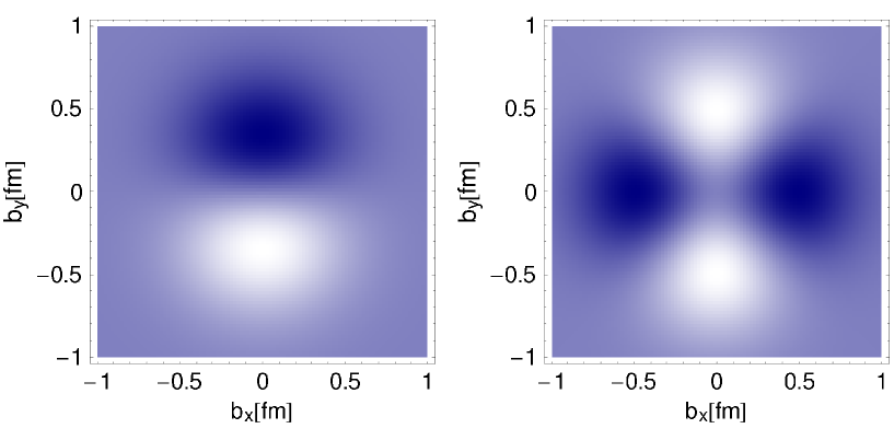
Figure 1: Density plots in the impact parameter plane for the functions $b\exp[-b^{2}/b_{0}^{2}]\sin\phi$ (left) and $b^{2}\exp[-b^{2}/b_{0}^{2}]\cos(2\phi)$ (right), with $b_{0}=0.5$ fm. These functions illustrate the terms in the quark density (8) which break rotational symmetry, as explained after (2). Dark areas represent high densities.

Integrating the densities (7) and (8) over all impact parameters one obtains generalized parton distributions in momentum space at $t=0$, namely

$$\int d^{2}\mbox{\boldmath{$b$}}\,\Big{[}F(x,\mbox{\boldmath{$b$}})+\lambda\tilde{F}(x,\mbox{\boldmath{$b$}})\Big{]}\>=\>H(x,0,0)+\lambda\Lambda\tilde{H}(x,0,0) = f_{1}(x)+\lambda\Lambda\,g_{1}(x)\;,$$ (12)

$$\int d^{2}\mbox{\boldmath{$b$}}\,\Big{[}F(x,\mbox{\boldmath{$b$}})+s^{i}F_{T}^{i}(x,\mbox{\boldmath{$b$}})\Big{]}\>=\>H(x,0,0)+s^{i}S^{i}\,H_{T}(x,0,0) = f_{1}(x)+s^{i}S^{i}\,h_{1}(x)\;.$$ (13)

Here we have used that GPDs in the forward limit $\xi=0$ and $t=0$ reduce to the usual parton densities, namely

$$H(x,0,0)=f_{1}(x),\qquad\qquad\tilde{H}(x,0,0)=g_{1}(x),\qquad\qquad H_{T}(x,0,0)=h_{1}(x)$$ (14)

for $x>0$, where $f_{1}$ denotes the unpolarized quark distribution, $g_{1}$ the quark helicity distribution, and $h_{1}$ the quark transversity distribution (another common notation is $f_{1}=q$, $g_{1}=\Delta q$ and $h_{1}=\delta q$). Corresponding relations involving antiquark distributions hold for $x<0$. Weighting the impact parameter distributions with $b^{2}$ before integration, one obtains derivatives at $t=0$,

$$\int d^{2}\mbox{\boldmath{$b$}}\;b^{2}\Big{(}F+\lambda\tilde{F}\Big{)} = \Bigg{[}4\frac{\partial}{\partial t}\Big{(}H+\lambda\Lambda\tilde{H}\Big{)}\Bigg{]}_{t=0}\;,$$ (15)

$$\int d^{2}\mbox{\boldmath{$b$}}\;b^{2}\Big{(}F+s^{i}F_{T}^{i}\Big{)} = \Bigg{[}4\frac{\partial}{\partial t}\Big{(}H+s^{i}S^{i}\Big{[}H_{T}-\frac{t}{4m^{2}}\tilde{H}_{T}\Big{]}\Big{)}\Bigg{]}_{t=0}\,,$$ (16)

where we use the subscript $t=0$ to indicate that the GPDs are taken in momentum space as in (2), with $\xi=0$ as always in this and the next section. The ratio of the integrals in (15) and (12) or in (16) and (13) thus gives the average squared impact parameter $b^{2}$ of quarks with given polarization and plus-momentum fraction. The average sideways shift in the impact parameter distribution due to the transverse polarization of either the quark or the proton is obtained from

$$\int d^{2}\mbox{\boldmath{$b$}}\;b^{j}\,\Big{(}F+s^{i}F_{T}^{i}\Big{)}=\Bigg{[}\frac{1}{2m}\Big{(}S^{i}\epsilon^{ij}E+s^{i}\epsilon^{ij}(E_{T}+2\tilde{H}_{T})\Big{)}\Bigg{]}_{t=0}$$ (17)

normalized to the integral in (13). This shift is more involved than in the case of longitudinally polarized or unpolarized quarks,

$$\int d^{2}\mbox{\boldmath{$b$}}\;b^{j}\,\Big{(}F+\lambda\tilde{F}\Big{)}=\int d^{2}\mbox{\boldmath{$b$}}\;b^{j}\,F=\Bigg{[}\frac{1}{2m}S^{i}\epsilon^{ij}E\,\Bigg{]}_{t=0}\;,$$ (18)

which has been discussed in some detail in [6]. Finally, the average distortion of the impact parameter density due to the last term in (8) is characterized by

$$\int d^{2}\mbox{\boldmath{$b$}}\;(2b^{j}b^{k}-b^{2}\delta^{jk})\,\Big{(}F+s^{i}F_{T}^{i}\Big{)}=\Bigg{[}\frac{1}{m^{2}}\,(s^{j}S^{k}+S^{j}s^{k}-s^{i}S^{i}\,\delta^{jk})\,\tilde{H}_{T}\,\Bigg{]}_{t=0}\,.$$ (19)

We note in (7) and (8) that there is no polarization effect in the impact parameter distributions for longitudinally polarized quarks in a transversely polarized proton and vice versa. This is because the only structures describing such effects which are allowed by parity conservation are $\lambda S^{i}b^{i}$ or $\Lambda s^{i}b^{i}$. They are odd under time reversal and hence forbidden. This corresponds to the fact that the generalized distributions $\tilde{E}$ and $\tilde{E}_{T}$ in (2) do not appear in the matrix elements at $\xi=0$, the former because it is multiplied with $\Delta^{+}=-2\xi P^{+}$ in its definition and the latter because it is an odd function of $\xi$ [9].

It is instructive to compare our impact parameter densities with the densities for quarks of definite light-cone momentum fraction $x$ and transverse momentum $k$, which play a prominent role in the description of spin asymmetries in a variety of hard processes. They can be defined from the correlation function

$$\Phi_{\alpha\beta}(x,\mbox{\boldmath{$k$}})=\int\frac{dz^{-}}{4\pi}\frac{d^{2}\mbox{\boldmath{$z$}}}{(2\pi)^{2}}\;e^{ixp^{+}z^{-}}e^{-i\mbox{\boldmath{$\scriptstyle k$}}\mbox{\boldmath{$\scriptstyle z$}}}\,\langle p|\,\bar{q}_{\beta}(-{\textstyle\frac{1}{2}}z)\,W[-{\textstyle\frac{1}{2}}z,{\textstyle\frac{1}{2}}z]\;q_{\alpha}({\textstyle\frac{1}{2}}z)|\,p\rangle\,\Big{|}_{z^{+}=0}\;,$$ (20)

where it is understood that the proton states have zero transverse momentum. The Wilson line $W$ has recently been recognized as essential in the definition, since different physical processes require different paths leading from $-{\textstyle\frac{1}{2}}z$ to ${\textstyle\frac{1}{2}}z$ and can actually give different correlation functions (see e.g. [18] and references therein). Physically, the gluons resummed in the Wilson lines describe interactions of spectator partons in the process where the correlation function appears, and the corresponding parton distributions describe the density of quarks or antiquarks in the presence of these interactions. This subtlety did not appear in the generalized parton distributions (2) and their impact parameter analogs, because there the quark field and its conjugate are separated by a light-like distance and the relevant Wilson line just runs along the light-cone between $-{\textstyle\frac{1}{2}}z$ and ${\textstyle\frac{1}{2}}z$. Projecting out densities for quarks of definite longitudinal or transverse polarization from (20), one obtains [19]

$$\frac{1}{2}\mathrm{Tr}\Big{[}(\gamma^{+}+\lambda\gamma^{+}\gamma_{5})\,\Phi\Big{]} = \frac{1}{2}\Bigg{[}f_{1}^{\phantom{\perp}\!\!}+S^{i}\epsilon^{ij}k^{j}\frac{1}{m}\,f_{1T}^{\perp}+\lambda\Lambda\,g_{1}^{\phantom{\perp\!\!}}+\lambda\,S^{i}k^{i}\frac{1}{m}\,g_{1T}^{\phantom{\perp\!\!}}\Bigg{]}\,,$$

$$\frac{1}{2}\mathrm{Tr}\Big{[}(\gamma^{+}-s^{j}i\sigma^{+j}\gamma_{5})\,\Phi\Big{]} = \frac{1}{2}\Bigg{[}f_{1}^{\phantom{\perp\!\!}}+S^{i}\epsilon^{ij}k^{j}\frac{1}{m}\,f_{1T}^{\perp}+s^{i}\epsilon^{ij}k^{j}\frac{1}{m}\,h_{1}^{\perp}+s^{i}S^{i}h_{1}^{\phantom{\perp\!\!}}$$ (21)

$$\hskip 6.99997pt{}+s^{i}(2k^{i}k^{j}-\mbox{\boldmath{$k$}}^{2}\delta^{ij})S^{j}\frac{1}{2m^{2}}\,h_{1T}^{\perp}+\Lambda\,s^{i}k^{i}\frac{1}{m}\,h_{1L}^{\perp}\Bigg{]}\,,$$

where we have used the notation of Boer, Mulders, Tangerman [20, 21] for the distribution functions, which depend on $x$ and $\mbox{\boldmath{$k$}}^{2}$. Integrating over $k$ one recovers the distributions $f_{1}(x)=\int d^{2}\mbox{\boldmath{$k$}}\,f_{1}(x,\mbox{\boldmath{$k$}}^{2})$, $g_{1}(x)=\int d^{2}\mbox{\boldmath{$k$}}\,g_{1}(x,\mbox{\boldmath{$k$}}^{2})$ and $h_{1}(x)=\int d^{2}\mbox{\boldmath{$k$}}\,h_{1}(x,\mbox{\boldmath{$k$}}^{2})$ we already encountered in (14). The tensor structures in (2) are analogs of those in (7) and (8), with $k$ taking the role of $b$. The corresponding analogy between transverse momentum dependent and impact parameter dependent distributions reads

$$f_{1}^{\phantom{\perp}}\leftrightarrow H,\hskip 93.00017ptf_{1T}^{\perp}\leftrightarrow{}-E^{\prime},\hskip 66.00015ptg_{1}^{\phantom{\perp}}\leftrightarrow\tilde{H},$$

$$h_{1}^{\phantom{\perp}}\leftrightarrow H_{T}-\Delta_{b}\tilde{H}_{T}/(4m^{2})\,,\qquad h_{1}^{\perp}\leftrightarrow{}-(E_{T}^{\prime}+2\tilde{H}_{T}^{\prime})\,,\qquad h_{1T}^{\perp}\leftrightarrow 2\tilde{H}_{T}^{\prime\prime}\,.$$ (22)

The impact parameter distributions which would correspond to $g_{1T}^{\phantom{\perp}}$ and $h_{1L}^{\perp}$ vanish because of time invariance, as discussed above. Notice that the momentum $k$ changes sign under time reversal, whereas the position vector $b$ does not. The structures $\lambda\,S^{i}k^{i}$ and $\Lambda\,s^{i}k^{i}$ describing polarization effects for longitudinally polarized quarks in a transversely polarized proton and vice versa are hence time reversal invariant. On the other hand, both $S^{i}\epsilon^{ij}k^{j}$ and $s^{i}\epsilon^{ij}k^{j}$ are odd under time reversal. The corresponding distributions $f_{1T}^{\perp}$ and $h_{1}^{\perp}$ (which respectively are the Sivers and Boer-Mulders functions) are however not constrained to be zero by time reversal invariance. This is because the Wilson line in the correlation function for relevant processes like semi-inclusive deep inelastic scattering or Drell-Yan pair production have paths that are not invariant under time reversal, contrary to the paths appearing in the impact parameter distributions discussed above. Time reversal thus connects transverse momentum dependent distributions with different Wilson lines, but does not constrain them to be zero [22]. We finally note that, beyond the formal correspondence of the functions $E(x,\mbox{\boldmath{$b$}})$ in (8) and $f_{1T}^{\perp}(x,\mbox{\boldmath{$k$}})$ in (2), a deep dynamical connection between them has recently been proposed in [23, 24].

We have seen in (12) to (19) how the impact parameter distributions can be reduced to distributions only depending on the momentum fraction $x$ by taking appropriate integrals over $b$. Conversely, one obtains distributions only depending on $b$ by integrating over $x$. Taking Mellin moments in $x$, we obtain expectation values of the well-known local twist-two operators in proton states localized at zero impact parameter,

$$(p^{+})^{n}\int_{-1}^{1}dx\,x^{n-1}F(x,\mbox{\boldmath{$b$}}) = \frac{1}{2}\,\mathcal{N}^{-1}\,\Big{\langle}p^{+},\mbox{\boldmath{$0$}}\,\Big{|}\,\bar{q}\gamma^{+}\,(i{D^{\raisebox{2.41112pt}{$\scriptstyle\leftrightarrow$}}}{}^{+})^{n-1}q\Big{|}\,p^{+},\mbox{\boldmath{$0$}}\Big{\rangle},$$

$$(p^{+})^{n}\int_{-1}^{1}dx\,x^{n-1}\tilde{F}(x,\mbox{\boldmath{$b$}}) = \frac{1}{2}\,\mathcal{N}^{-1}\,\Big{\langle}p^{+},\mbox{\boldmath{$0$}}\,\Big{|}\,\bar{q}\gamma^{+}\gamma_{5}\,(i{D^{\raisebox{2.41112pt}{$\scriptstyle\leftrightarrow$}}}{}^{+})^{n-1}q\Big{|}\,p^{+},\mbox{\boldmath{$0$}}\Big{\rangle},$$

$$(p^{+})^{n}\int_{-1}^{1}dx\,x^{n-1}F_{T}^{j}(x,\mbox{\boldmath{$b$}}) = {}-\frac{i}{2}\,\mathcal{N}^{-1}\,\Big{\langle}p^{+},\mbox{\boldmath{$0$}}\,\Big{|}\,\bar{q}\sigma^{+j}\gamma_{5}\,(i{D^{\raisebox{2.41112pt}{$\scriptstyle\leftrightarrow$}}}{}^{+})^{n-1}q\Big{|}\,p^{+},\mbox{\boldmath{$0$}}\Big{\rangle},$$ (23)

where ${D^{\raisebox{2.41112pt}{$\scriptstyle\leftrightarrow$}}}{}^{\mu}={\textstyle\frac{1}{2}}({D^{\raisebox{2.41112pt}{$\scriptstyle\rightarrow$}}}{}^{\mu}-{D^{\raisebox{2.41112pt}{$\scriptstyle\leftarrow$}}}{}^{\mu})={\textstyle\frac{1}{2}}(\hskip 0.2pt{\partial^{\raisebox{2.41112pt}{$\scriptstyle\rightarrow$}}}{}^{\mu}-{\partial^{\raisebox{2.41112pt}{$\scriptstyle\leftarrow$}}}{}^{\mu})-igA^{\mu}$, and all field operators are to be taken at position $z$ with $z^{+}=z^{-}=0$ and $\mbox{\boldmath{$z$}}=\mbox{\boldmath{$b$}}$. To obtain matrix elements of local operators, one has to integrate over both positive and negative $x$ and hence not only combines the information from different momentum fractions but also from quarks and antiquarks. According to the charge conjugation properties we discussed after (7) and (8), moments with odd $n$ in (2) correspond to the sum of quark and antiquark densities for $\tilde{F}$ and to their difference for $F$ and $F_{T}^{j}$, whereas for moments with even $n$ the situation is reversed. The lowest $x$ moments of $F$ and ${\textstyle\frac{1}{2}}[F+s^{i}F_{T}^{i}]$ hence describe the transverse distribution of unpolarized and transversely polarized quarks minus antiquarks in the proton, respectively. Higher $x$ moments give the transverse distributions of quarks plus or minus antiquarks weighted with a power of their plus-momentum fraction. In contrast, the $x$ moments of ${\textstyle\frac{1}{2}}[F+\lambda\tilde{F}]$ describe the transverse distribution of quarks plus or minus antiquarks with chirality $\lambda$ (i.e. quarks with helicity $\lambda$ and antiquarks with helicity $-\lambda$). A two-dimensional Fourier transform turns the expectation values (2) into matrix elements for proton states of definite momenta, which are parameterized by form factors depending on the squared momentum transfer $t$. These form factors can be evaluated in lattice QCD since the corresponding operators are local and thus allow continuation into Euclidean space. It is amusing that after a Fourier transform they become quantities (2) whose physical interpretation is naturally given in a light-cone framework.

Note that our interpretation of form factors differs from the well-known interpretation due to Sachs [25], where their three-dimensional Fourier transforms yield densities in a static proton state. That framework has been extended to generalized parton distributions as functions of $x$, $\xi$ and $t$ in [26]. It is limited by ambiguities due to the impossibility to localize a particle more accurately than within its Compton wavelength. Localization in only two dimensions is not affected by this limitation, and the wave packets (3) are indeed eigenstates of a two-dimensional position operator [17]. The price to pay for this is the loss of manifest three-dimensional rotation invariance in the light-cone framework. In return, the mixed representation of position space in two dimensions and plus-momentum in the third allows one to boost to a frame where the proton moves fast, which is a natural frame for the physical interpretation of quark and antiquark degrees of freedom.

So far we have interpreted ${\textstyle\frac{1}{2}}[F+s^{i}F_{T}^{i}]$ in (8) as the density of quarks with a given transverse polarization $s$. The vector field $\mbox{\boldmath{$F$}}_{\!T}(x,\mbox{\boldmath{$b$}})$ gives the direction in which the transverse polarization of quarks is largest, and its size $|\mbox{\boldmath{$F$}}_{\!T}(x,\mbox{\boldmath{$b$}})|$ is the difference of densities with quarks polarized along or opposite to this direction. According to (8) we can write $F_{T}^{i}$ as the superposition of three terms, given by functions of $\mbox{\boldmath{$b$}}^{2}$ times the vectors $S^{i}$, $\epsilon^{ij}b^{j}$ and $(2b^{i}b^{j}-b^{2}\delta^{ij})S^{j}$. The field lines of the term with $\epsilon^{ij}b^{j}$ are circles around the origin, and those of the term with $(2b^{i}b^{j}-b^{2}\delta^{ij})S^{j}$ are circles going through the origin with a tangent along the proton polarization $S^{i}$, as illustrated in Fig. 2.

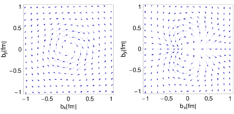
Figure 2: The vector fields $\epsilon^{ij}b^{j}\exp[-b^{2}/b_{0}^{2}]$ (left) and $(2b^{i}b^{j}-b^{2}\delta^{ij})S^{j}\exp[-b^{2}/b_{0}^{2}]$ (right) with $S^{i}$ along the $x$-axis and $b_{0}=0.5$ fm. They illustrate the form of two terms in the decomposition of $F_{T}^{i}(x,\mbox{\boldmath{$b$}})$, which describes the transverse polarization of quarks in the impact parameter plane. The third term in the decomposition is a field parallel to $S^{i}$.

The divergence and the curl of the field $F_{T}^{i}(x,\mbox{\boldmath{$b$}})$ respectively are

$$\frac{\partial}{\partial b^{i}}F_{T}^{i} = 2S^{i}b^{i}H_{T}^{\prime}\,,$$

$$\frac{\partial}{\partial b^{i}}\epsilon^{ij}F_{T}^{j} = \frac{1}{2m}\Delta_{b}\Big{(}E_{T}+2\tilde{H}_{T}\Big{)}-2S^{i}\epsilon^{ij}b^{j}\frac{\partial}{\partial b^{2}}\Big{(}H_{T}-\frac{1}{2m^{2}}\Delta_{b}\tilde{H}_{T}\Big{)}\,.$$ (24)

They can be rewritten as matrix elements of operators which are total derivatives. This is readily seen in Mellin space, where we have

$$(p^{+})^{n}\int_{-1}^{1}dx\,x^{n-1}\frac{\partial}{\partial b^{i}}F_{T}^{i}(x,\mbox{\boldmath{$b$}}) = {}-\frac{i}{2}\,\mathcal{N}^{-1}\,\Big{\langle}p^{+},\mbox{\boldmath{$0$}}\,\Big{|}\,\partial_{\mu}\Big{[}\bar{q}\sigma^{+\mu}\gamma_{5}\,(i{D^{\raisebox{2.41112pt}{$\scriptstyle\leftrightarrow$}}}{}^{+})^{n-1}q\Big{]}\,\Big{|}\,p^{+},\mbox{\boldmath{$0$}}\Big{\rangle}\,,$$

$$(p^{+})^{n}\int_{-1}^{1}dx\,x^{n-1}\frac{\partial}{\partial b^{i}}\epsilon^{ij}F_{T}^{j}(x,\mbox{\boldmath{$b$}}) = \frac{1}{2}\,\mathcal{N}^{-1}\,\Big{\langle}p^{+},\mbox{\boldmath{$0$}}\,\Big{|}\,\partial_{\mu}\Big{[}\bar{q}\sigma^{+\mu}(i{D^{\raisebox{2.41112pt}{$\scriptstyle\leftrightarrow$}}}{}^{+})^{n-1}q\Big{]}\,\Big{|}\,p^{+},\mbox{\boldmath{$0$}}\Big{\rangle}\,,$$ (25)

with all field operators evaluated at $z^{+}=z^{-}=0$ and $\mbox{\boldmath{$z$}}=\mbox{\boldmath{$b$}}$. To obtain (2) we have used the representation (2) and the fact that the first term in $\partial^{+}[\bar{q}\sigma^{+-}\ldots q]+\partial_{i}[\bar{q}\sigma^{+i}\ldots q]=\partial_{\mu}[\bar{q}\sigma^{+\mu}\ldots q]$ vanishes when taking a matrix element between states of equal plus-momentum. The operators in (2) can be rewritten using the equations of motion as we will discuss in Sect. 4.

The Mellin moments of the impact parameter distributions $H(x,b^{2})$, $E(x,b^{2})$ etc. are Fourier transforms of form factors in momentum space, which are denoted by

$$A_{n0}(t) = \int_{-1}^{1}dx\,x^{n-1}H(x,0,t),\qquad\hskip 10.50005ptB_{n0}(t)\>=\>\int_{-1}^{1}dx\,x^{n-1}E(x,0,t),$$

$$A_{Tn0}(t) = \int_{-1}^{1}dx\,x^{n-1}H_{T}(x,0,t),\qquad B_{Tn0}(t)\>=\>\int_{-1}^{1}dx\,x^{n-1}E_{T}(x,0,t),$$

$$\tilde{A}_{Tn0}(t) = \int_{-1}^{1}dx\,x^{n-1}\tilde{H}_{T}(x,0,t)$$ (26)

in a standard notation (see Sect. 4). These form factors can be calculated in lattice QCD [11, 12, 13], where it has become customary to fit them to a dipole form. For reasons that will be clear shortly, let us consider the more general power-law ansatz

$$A(t)=\frac{A(0)}{(1-{t/m_{A\hskip 0.6pt}^{2}})^{\hskip 1.0ptp}_{\phantom{d}}\rule{0.0pt}{10.00002pt}}\>,$$ (27)

where the power $p$ and the mass $m_{A\hskip 0.6pt}$ are free parameters for a given form factor $A(t)$. Note that in the limit $p\to\infty$ at fixed $m_{A\hskip 0.6pt}^{2}/p$ this ansatz gives an exponential in $t$. The Fourier transformation of (27) to impact parameter space leads to the modified Bessel function,

$$A(b^{2})=C\;(m_{A\hskip 0.6pt}b)^{p-1}K_{p-1}(m_{A\hskip 0.6pt}b)\,,\qquad\qquad C=\frac{m_{A\hskip 0.6pt}^{2}}{2^{p}\pi\Gamma(p)}\,A(0)\,,$$ (28)

and the derivatives defined in (9) and (10) are

$$A^{\prime}(b^{2}) = -{\textstyle\frac{1}{2}}Cm_{A\hskip 0.6pt}^{2}\,(m_{A\hskip 0.6pt}b)^{p-2}K_{p-2}(m_{A\hskip 0.6pt}b)\,,\qquad\qquad A^{\prime\prime}(b^{2})={\textstyle\frac{1}{4}}Cm_{A\hskip 0.6pt}^{4}\,(m_{A\hskip 0.6pt}b)^{p-3}K_{p-3}(m_{A\hskip 0.6pt}b)\,,$$

$$\Delta_{b}A(b^{2}) = -Cm_{A\hskip 0.6pt}^{2}\,(m_{A\hskip 0.6pt}b)^{p-2}\Big{[}2K_{p-2}(m_{A\hskip 0.6pt}b)-m_{A\hskip 0.6pt}b\,K_{p-3}(m_{A\hskip 0.6pt}b)\,\Big{]}\,.$$ (29)

A parameterization of the type (27) is in the first instance only valid in the $t$ range where the form factor has been fitted. In particular, lattice computations have an upper limit $|t|_{\mathrm{max}}$ on the squared momentum transfer given by the lattice parameters. This corresponds to a limited resolution of order $(|t|_{\mathrm{max}})^{-1/2}$ on the impact parameter [16]. Furthermore, results obtained on a finite lattice cannot give direct information on the behavior of quark densities at impact parameters much larger than the lattice size. Nevertheless, one may want to require that a parameterization leads at least to a physically plausible behavior of the impact parameter density at small and large $b$. To analyze this behavior we need the relations

$$K_{0}(z) \mathrel{\mathop{\sim}\limits_{z\to 0}} \log\frac{2}{z},\qquad\qquad K_{p}(z)\>\>\>\mathrel{\mathop{\sim}\limits_{z\to 0}}\>\>\>\frac{2^{p-1}\Gamma(p)}{z^{p}}\qquad\mbox{for $p>0$},$$

$$K_{p}(z) \mathrel{\mathop{\sim}\limits_{z\to\infty}} e^{-z}\sqrt{\frac{\pi}{2z}}$$ (30)

and $K_{-p}(z)=K_{p}(z)$. At large $b$, each term in the Mellin moments of the densities (7) and (8) then falls off like $(m_{A\hskip 0.6pt}b)^{p-3/2}\,e^{-m_{A\hskip 0.6pt}b}$. For the limit $b\to 0$ it seems reasonable to require a regular behavior of the impact parameter density, which implies that no term should diverge and that $b^{j}E^{\prime}$, $b^{j}(E_{T}^{\prime}+2\tilde{H}_{T}^{\prime})$ and $(2b^{i}b^{j}-b^{2}\delta^{ij})\tilde{H}_{T}^{\prime\prime}$ should vanish at $b=0$, since they have a nontrivial dependence on the azimuthal angle $\phi$. This restricts $p$ in the parameterization of moments to $p>1$ for $H$, $\tilde{H}$ and $H_{T}$, to $p>3/2$ for $E$ and $E_{T}$, and to $p>2$ for $\tilde{H}_{T}$. The terms with $H$, $\tilde{H}$, $H_{T}$ and $\Delta_{b}\tilde{H}_{T}$ in the moments of (7) and (8) then all take finite values at $b=0$. In momentum space these restrictions are tantamount to requiring that the Mellin moments of $F(x,0,t)$, $\tilde{F}(x,0,t)$, $F_{T}^{j}(x,0,t)$ decrease faster than $1/t$ for $t\to-\infty$, as is readily seen when the proton spinor products in (2) are evaluated [9]. Note in particular that a dipole ansatz with $p=2$ for $\tilde{A}_{Tn0}(t)$ gives only a $1/t$ falloff in the $n$th moment of $F_{T}^{i}(x,0,t)$ and a corresponding logarithmic divergence at $b=0$ in the $n$th moment of $F_{T}^{i}(x,\mbox{\boldmath{$b$}})$.

To illustrate how the transverse spin density in the proton may look like, we focus now on the first moment ${\textstyle\frac{1}{2}}\int_{-1}^{1}dx\,[F(x,\mbox{\boldmath{$b$}})+s^{i}F_{T}^{i}(x,\mbox{\boldmath{$b$}})]$, which gives the difference of impact parameter densities for quarks and antiquarks (for ease of language we will simply speak of quarks in the following). As a numerical example we take a parameterization (27) with $p=2$ for $A_{10}(t)$, $B_{10}(t)$, $A_{T10}(t)$ and $p=3$ for $B_{T10}(t)$, $\tilde{A}_{T10}(t)$. We set the mass parameters $m_{A\hskip 0.6pt}$ to $1$ GeV for $A_{10}(t)$, $B_{10}(t)$ and to $1.5$ GeV for the three other form factors, and take

$$A_{10}(0)=2,\qquad B_{10}(0)=3,\qquad A_{T10}(0)=1,\qquad B_{T10}(0)=6,\qquad\tilde{A}_{T10}(0)=-1$$ (31)

for their values at $t=0$. This set of parameterizations is a rough approximation of preliminary results from lattice calculations [27] for the first moments of generalized $u$-quark distributions (where $|t|$ goes up to about $3.5\,\mbox{GeV}^{2}\approx(0.1\,\mbox{fm})^{-2}$ and lattice sizes are between $1.5$ and $2.2$ fm). We stress that it is meant to be indicative and not a precise representation of those results. We note that $A_{10}(0)=2$ correctly gives the number of valence $u$-quarks in the proton, whereas $B_{10}(0)=3$ is too large compared with the value $1.67$ one obtains from the measured magnetic moments of proton and neutron (recall that $B_{10}(t)$ is the relevant quark flavor contribution to the electromagnetic Pauli form factor).

In Fig. 3 we show the resulting first moment of the impact parameter density for unpolarized quarks in a transversely polarized proton and for transversely polarized quarks in an unpolarized proton. The dipole-type structures due to $S^{i}\epsilon^{ij}b^{j}E^{\prime}$ and $s^{i}\epsilon^{ij}b^{j}(E_{T}^{\prime}+2\tilde{H}_{T}^{\prime})$ are clearly visible, reflecting the large values in (31) for $B_{10}$ and $B_{T10}+2\tilde{A}_{T10}$ at $t=0$. The sum of both dipoles dominates the structure of the distribution for transverse polarization of both quark and proton, as is seen in Fig. 4, whereas the quadrupole-type term $s^{i}(2b^{i}b^{j}-b^{2}\delta^{ij})S^{j}\tilde{H}_{T}^{\prime\prime}$ is less prominent in our numerical example. We note that the two dipoles terms $S^{i}\epsilon^{ij}b^{j}E^{\prime}$ and $s^{i}\epsilon^{ij}b^{j}(E_{T}^{\prime}+2\tilde{H}_{T}^{\prime})$ tend to cancel if quark and proton spin are opposite to each other, and the resulting density (not shown here) is rather sensitive to the precise values in the form factor parameterizations. Figure 5 finally shows the lowest moment of the vector field $F^{i}_{T}(x,\mbox{\boldmath{$b$}})$ describing the transverse quark polarization in a proton with or without transverse polarization.

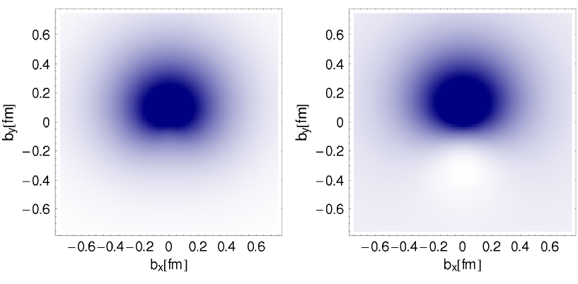
Figure 3: Left: Illustration of the first moment $\int_{-1}^{1}dx\,F(x,\mbox{\boldmath{$b$}})$ of the impact parameter density for unpolarized $u$-quarks in a proton with transverse spin vector $\mbox{\boldmath{$S$}}=(1,0)$. Right: The same for the first moment ${\textstyle\frac{1}{2}}\int_{-1}^{1}dx\,[F(x,\mbox{\boldmath{$b$}})+s^{i}F_{T}^{i}(x,\mbox{\boldmath{$b$}})]$ of the distribution of $u$-quarks with transverse spin vector $\mbox{\boldmath{$s$}}=(1,0)$ in an unpolarized proton. Dark areas represent the highest and light areas the lowest values of the density. Further explanation is given in the text.

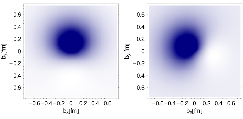
Figure 4: Illustration of the lowest moment ${\textstyle\frac{1}{2}}\int_{-1}^{1}dx\,[F(x,\mbox{\boldmath{$b$}})+s^{i}F^{i}_{T}(x,\mbox{\boldmath{$b$}})]$ for $u$-quarks in a proton with transverse spin vector $\mbox{\boldmath{$S$}}=(1,0)$. The transverse quark spin vector is $\mbox{\boldmath{$s$}}=(1,0)$ in the left plot and $\mbox{\boldmath{$s$}}=(0,1)$ in the right plot.

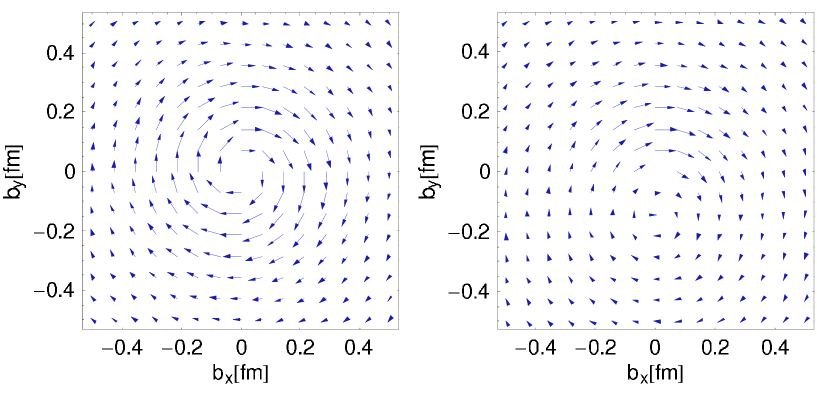
Figure 5: Illustration of the lowest moment $\int_{-1}^{1}dx\,F^{i}_{T}(x,\mbox{\boldmath{$b$}})$ of the vector field describing the transverse polarization of $u$-quarks in an unpolarized proton (left) and in a proton with transverse spin in the $x$-direction (right).

3 The spin matrix and positivity constraints

In the previous section we have discussed the density of quarks with transverse or longitudinal polarization in a transversely or longitudinally polarized proton. Densities for arbitrary polarization states can be obtained from the spin matrix in the light-cone helicity basis

$$M_{(\Lambda^{\prime}\lambda^{\prime})(\Lambda\lambda)}(x,\mbox{\boldmath{$b$}})=\mathcal{N}^{-1}\,\int\frac{dz^{-}}{4\pi}\,e^{ixp^{+}z^{-}}\,\Big{\langle}p^{+},\mbox{\boldmath{$0$}},\Lambda^{\prime}\,\Big{|}\,\bar{q}(z_{2})\Gamma_{\lambda^{\prime}\lambda}\,q(z_{1})\Big{|}\,p^{+},\mbox{\boldmath{$0$}},\Lambda\Big{\rangle}$$ (32)

with $z_{1}^{+}=z_{2}^{+}=0$, $\mbox{\boldmath{$z$}}_{1}=\mbox{\boldmath{$z$}}_{2}=\mbox{\boldmath{$b$}}$, and $z_{1}^{-}=-z_{2}^{-}={\textstyle\frac{1}{2}}z^{-}$. Here $\Lambda^{\prime}$ and $\Lambda$ denote light-cone helicities of the proton states, and definite light-cone helicities $\lambda^{\prime}$ and $\lambda$ of the quark are projected out by the Dirac matrices (see e.g. [9])

$$\Gamma_{++}=\gamma^{+}(1+\gamma_{5}), \qquad\qquad\Gamma_{-+}=-i\sigma^{+1}(1+\gamma_{5}),$$

$$\Gamma_{--}=\gamma^{+}(1-\gamma_{5}), \qquad\qquad\Gamma_{+-}=i\sigma^{+1}(1-\gamma_{5}).$$ (33)

The corresponding labeling of helicities in a handbag graph is shown in Fig. 6a. The matrix $M_{(\Lambda^{\prime}\lambda^{\prime})(\Lambda\lambda)}$ reads

$$\left(\begin{array}[]{cccc}H+\tilde{H}&-ie^{-i\phi}\displaystyle\frac{b}{m}E^{\prime}&ie^{i\phi}\displaystyle\frac{b}{m}\Big{(}E_{T}^{\prime}+2\tilde{H}_{T}^{\prime}\Big{)}&2\Big{(}H_{T}-\displaystyle\frac{1}{4m^{2}}\Delta_{b}\tilde{H}_{T}\Big{)}\\ ie^{i\phi}\displaystyle\frac{b}{m}E^{\prime}&H-\tilde{H}&2e^{2i\phi}\displaystyle\frac{b^{2}}{m^{2}}\tilde{H}_{T}^{\prime\prime}&ie^{i\phi}\displaystyle\frac{b}{m}\Big{(}E_{T}^{\prime}+2\tilde{H}_{T}^{\prime}\Big{)}\\ -ie^{-i\phi}\displaystyle\frac{b}{m}\Big{(}E_{T}^{\prime}+2\tilde{H}_{T}^{\prime}\Big{)}&2e^{-2i\phi}\displaystyle\frac{b^{2}}{m^{2}}\tilde{H}_{T}^{\prime\prime}&H-\tilde{H}&-ie^{-i\phi}\displaystyle\frac{b}{m}E^{\prime}\\ 2\Big{(}H_{T}-\displaystyle\frac{1}{4m^{2}}\Delta_{b}\tilde{H}_{T}\Big{)}&-ie^{-i\phi}\displaystyle\frac{b}{m}\Big{(}E_{T}^{\prime}+2\tilde{H}_{T}^{\prime}\Big{)}&ie^{i\phi}\displaystyle\frac{b}{m}E^{\prime}&H+\tilde{H}\end{array}\right)$$ (39)

if we order the proton-quark helicity combinations as $(\Lambda\lambda)=(++),(-+),(+-),(--)$. Here GPDs are given in impact parameter space with the notation specified after (8), and the azimuthal angle $\phi$ of $b$ is defined after (2). The quark density for an arbitrary polarization state of proton and quark can be written as ${\textstyle\frac{1}{2}}\sum_{\Lambda^{\prime}\lambda^{\prime}\Lambda\lambda}\,(c_{\Lambda^{\prime}\lambda^{\prime}\phantom{\!\!\!\!\!()}})^{*}M_{(\Lambda^{\prime}\lambda^{\prime})(\Lambda\lambda)}\,c_{\Lambda\lambda\phantom{\!\!\!\!\!()}}$ with coefficients normalized to $\sum_{\Lambda\lambda}|c_{\Lambda\lambda}|^{2}=1$. This implies that the matrix $M_{(\Lambda^{\prime}\lambda^{\prime})(\Lambda\lambda)}$ must be positive semidefinite. Integration of (39) over $b$ leads to the known spin matrix for the forward distribution functions $f_{1}(x)$, $g_{1}(x)$, $h_{1}(x)$ according to (14), and the positivity of the corresponding eigenvalues gives immediately the Soffer bound $2|h_{1}(x)|\leq f_{1}(x)+g_{1}(x)$. Using the relations (2) we see that the matrix (39) of impact parameter dependent distributions is the exact analog of the spin matrix for transverse momentum dependent distribution functions, which was discussed in [28].

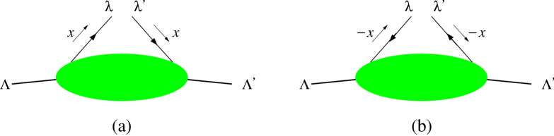
Figure 6: Labeling of the proton and parton helicities in the matrix elements $M_{(\Lambda^{\prime}\lambda^{\prime})(\Lambda\lambda)}$ in the quark region $x>0$ (a) and the antiquark region $x<0$ (b).

In order to simplify the following discussion, we change basis by multiplying (39) with the diagonal matrix $D=\mathrm{diag}(1,ie^{i\phi},-ie^{-i\phi},1)$ from the right and with $D^{\dagger}$ from the left. This gives a matrix

$$\left(\begin{array}[]{cccc}H+\tilde{H}&\displaystyle\frac{b}{m}E^{\prime}&\displaystyle\frac{b}{m}\Big{(}E_{T}^{\prime}+2\tilde{H}_{T}^{\prime}\Big{)}&2\Big{(}H_{T}-\displaystyle\frac{1}{4m^{2}}\Delta_{b}\tilde{H}_{T}\Big{)}\\ \displaystyle\frac{b}{m}E^{\prime}&H-\tilde{H}&-2\displaystyle\frac{b^{2}}{m^{2}}\tilde{H}_{T}^{\prime\prime}&\displaystyle\frac{b}{m}\Big{(}E_{T}^{\prime}+2\tilde{H}_{T}^{\prime}\Big{)}\\ \displaystyle\frac{b}{m}\Big{(}E_{T}^{\prime}+2\tilde{H}_{T}^{\prime}\Big{)}&-2\displaystyle\frac{b^{2}}{m^{2}}\tilde{H}_{T}^{\prime\prime}&H-\tilde{H}&\displaystyle\frac{b}{m}E^{\prime}\\ 2\Big{(}H_{T}-\displaystyle\frac{1}{4m^{2}}\Delta_{b}\tilde{H}_{T}\Big{)}&\displaystyle\frac{b}{m}\Big{(}E_{T}^{\prime}+2\tilde{H}_{T}^{\prime}\Big{)}&\displaystyle\frac{b}{m}E^{\prime}&H+\tilde{H}\;,\end{array}\right)$$ (40)

which is purely real and depends on $b$ but no longer on $\phi$. Positivity of the upper left $2\times 2$ sub-matrix of (40) leads to the bound

$$\frac{b}{m}\,|E^{\prime}|\leq\sqrt{H^{2}-\tilde{H}^{2}},$$ (41)

which has been discussed in [29]. Using the eigenvalues of the full matrix (40), we can tighten these bounds by including the tensor GPDs. With the abbreviations

$$a_{\pm} = H\pm\Big{(}H_{T}+\frac{1}{m^{2}}\tilde{H}_{T}^{\prime}-\frac{1}{2m^{2}}\Delta_{b}\tilde{H}_{T}\Big{)}\;,$$

$$b_{\pm} = \tilde{H}\pm\Big{(}H_{T}-\frac{1}{m^{2}}\tilde{H}_{T}^{\prime}\Big{)}\;,$$

$$c_{\pm} = \frac{b}{m}\Big{(}E^{\prime}\pm E_{T}^{\prime}\pm 2\tilde{H}_{T}^{\prime}\Big{)}$$ (42)

the four eigenvalues read

$$a_{+}+\sqrt{b_{+}^{2}+c_{+}^{2}}\,,\qquad a_{+}-\sqrt{b_{+}^{2}+c_{+}^{2}}\,,\qquad a_{-}+\sqrt{b_{-}^{2}+c_{-}^{2}}\,,\qquad a_{-}-\sqrt{b_{-}^{2}+c_{-}^{2}}\,.$$ (43)

We see that they are related pairwise by changing the sign of all chiral-odd distributions. This is tantamount to multiplying the matrix (40) with $\mathrm{diag}(1,1,-1,-1)$ from the left and from the right, which does of course not change its eigenvalues. Positivity of the eigenvalues (43) gives the bounds

$$0\>\leq\>a_{\pm}\,,\qquad\qquad c_{\pm}^{2}\>\leq\>a_{\pm}^{2}-b_{\pm}^{2}\>=\>(a_{\pm}+b_{\pm})(a_{\pm}-b_{\pm})\,,$$ (44)

which in particular imply $0\leq a_{\pm}+b_{\pm}$ and $0\leq a_{\pm}-b_{\pm}$. They explicitely read

$$\Big{|}\,H_{T}+\frac{1}{m^{2}}\tilde{H}_{T}^{\prime}-\frac{1}{2m^{2}}\Delta_{b}\tilde{H}_{T}\,\Big{|}\leq H$$ (45)

and

$$\frac{b^{2}}{m^{2}}\Big{(}E^{\prime}\pm E_{T}^{\prime}\pm 2\tilde{H}_{T}^{\prime}\Big{)}^{2} \leq \Big{(}H\pm H_{T}\pm\frac{1}{m^{2}}\tilde{H}_{T}^{\prime}\mp\frac{1}{2m^{2}}\Delta_{b}\tilde{H}_{T}\Big{)}^{2}-\Big{(}\tilde{H}\pm H_{T}\mp\frac{1}{m^{2}}\tilde{H}_{T}^{\prime}\Big{)}^{2}\,.\hskip 10.00002pt$$ (46)

In the phenomenological study [30] it was found that the bound (41) can indeed be very restrictive (and thus helpful) in reconstructing generalized parton distributions from experimental data. The tighter bounds (45) and (46) may therefore be of practical value even with limited information on the three additional chiral-odd distributions they contain. As in the case of the usual parton distributions, renormalization of the operators in (32) may destroy the density interpretation of the impact parameter distributions. Closer analysis reveals that the bounds following from positivity of the matrix $M_{(\Lambda^{\prime}\lambda^{\prime})(\Lambda\lambda)}$ should be valid at a sufficiently high renormalization scale $\mu^{2}$ [31]. They are stable under leading order evolution to higher scales, as shown in [32].

Since both experimental information and results from lattice QCD calculations are in the first instance given as a function of $t$, it is useful to have bounds also directly in momentum space. This can be achieved by applying to (46) the method used in [29] for the simpler bound (41), where the main ingredient is the Schwarz inequality. A method leading to the same results is to multiply (40) from the left and the right with $\mathrm{diag}(1,mb,mb,1)$. In the resulting matrix $\widehat{M}$ only even powers of $b$ appear. Integrating over $b$ as $2\pi\int_{0}^{\infty}db\,b\,\widehat{M}(b^{2})=\int d^{2}\mbox{\boldmath{$b$}}\,\widehat{M}(b^{2})$, one obtains GPDs and their derivatives at zero momentum transfer $t=0$. The result is still a positive semidefinite matrix, whose eigenvalues have the form (43) with

$$a_{\pm} = \Big{[}\,H+\tilde{H}+4m^{2}\frac{\partial}{\partial t}(H-\tilde{H})\pm 2(H_{T}-2\tilde{H}_{T})\,\Big{]}_{t=0}\;,$$

$$b_{\pm} = \Big{[}\,H+\tilde{H}-4m^{2}\frac{\partial}{\partial t}(H-\tilde{H})\pm 2(H_{T}+2\tilde{H}_{T})\,\Big{]}_{t=0}\;,$$

$$c_{\pm} = \Big{[}\,2(E\pm E_{T}\pm 2\tilde{H}_{T})\,\Big{]}_{t=0}\;.\phantom{\frac{\partial}{\partial t}}$$ (47)

This leads to the bounds

$$\Bigg{[}\Big{(}E\pm E_{T}\pm 2\tilde{H}_{T}\Big{)}^{2}\,\Bigg{]}_{t=0}\leq\Bigg{[}\Big{(}H+\tilde{H}\pm 2H_{T}\Big{)}\,\Big{(}4m^{2}\frac{\partial}{\partial t}(H-\tilde{H})\mp 4\tilde{H}_{T}\Big{)}\,\Bigg{]}_{t=0}\,,$$ (48)

where both expressions in large parentheses on the right-hand side must be positive or zero according to our remark after (44). The condition $0\leq[H+\tilde{H}\pm 2H_{T}]_{t=0}$ is just the Soffer bound.

Alternatively, we can multiply the matrix (40) from the left and the right with $\mathrm{diag}(mb,1,1,mb)$ and then integrate over $b$ as described above. The eigenvalues have again the structure of (43), and we obtain bounds

$$\Bigg{[}\Big{(}E\pm E_{T}\pm 2\tilde{H}_{T}\Big{)}^{2}\,\Bigg{]}_{t=0}\leq\Bigg{[}\Big{(}H-\tilde{H}\mp\frac{1}{2m^{2}}\int_{-\infty}^{t}dt^{\prime}\,\tilde{H}_{T}(t^{\prime})\Big{)}\,\Big{(}4m^{2}\frac{\partial}{\partial t}(H+\tilde{H}\pm 2H_{T})\mp 2\tilde{H}_{T}\Big{)}\,\Bigg{]}_{t=0}$$ (49)

with both expressions in large parentheses on the right-hand side positive or zero. They contain a function which is non-local in momentum space, namely

$$\int_{-\infty}^{0}dt\tilde{H}_{T}(t)=4\pi\tilde{H}_{T}(b=0),$$ (50)

which can be traced back to the integral $\int d^{2}\mbox{\boldmath{$b$}}\;b^{2}\tilde{H}_{T}^{\prime\prime}(b^{2})$ in the derivation.

For reasons which will become clear shortly, certain applications require bounds which do not involve the distribution $\tilde{H}$ . One such bound is simply obtained by omitting the last term in (46), which together with (45) leads to

$$\frac{b}{m}\,\Big{|}E^{\prime}\pm E_{T}^{\prime}\pm 2\tilde{H}_{T}^{\prime}\Big{|} \leq H\pm\Big{(}H_{T}+\frac{1}{m^{2}}\tilde{H}_{T}^{\prime}-\frac{1}{2m^{2}}\Delta_{b}\tilde{H}_{T}\Big{)}\,.$$ (51)

To obtain a bound in momentum space we multiply (51) with $mb$, integrate over $b$, and use the Schwarz inequality in the forms $\int d^{2}\mbox{\boldmath{$b$}}\,f\leq\int d^{2}\mbox{\boldmath{$b$}}\,|f|$ and $\int d^{2}\mbox{\boldmath{$b$}}\,b\,g\leq(\int d^{2}\mbox{\boldmath{$b$}}\,g)^{1/2}\,(\int d^{2}\mbox{\boldmath{$b$}}\,b^{2}g)^{1/2}$, following the method of [29]. This leads to

$$\Bigg{[}\Big{(}E\pm E_{T}\pm 2\tilde{H}_{T}\Big{)}^{2}\,\Bigg{]}_{t=0}\leq\Bigg{[}\Big{(}H\pm H_{T}\mp\frac{1}{4m^{2}}\int_{-\infty}^{t}dt^{\prime}\,\tilde{H}_{T}(t^{\prime})\Big{)}\,\Big{(}4m^{2}\frac{\partial}{\partial t}(H\pm H_{T})\mp 3\tilde{H}_{T}\Big{)}\,\Bigg{]}_{t=0}\;,\hskip 10.00002pt$$ (52)

where both terms in large parentheses on the right-hand side must be positive or zero. Alternatively one can add to (40) the positive semidefinite matrix

$$\left(\begin{array}[]{cccc}H-\tilde{H}&\displaystyle\frac{b}{m}E^{\prime}&0&0\\ \displaystyle\frac{b}{m}E^{\prime}&H+\tilde{H}&0&0\\ 0&0&H+\tilde{H}&\displaystyle\frac{b}{m}E^{\prime}\\ 0&0&\displaystyle\frac{b}{m}E^{\prime}&H-\tilde{H}\end{array}\right)$$ (53)

and proceed as above. One then obtains bounds analogous to (46) and to (48) and (49) by the replacements $H\to 2H$, $E\to 2E$, $\tilde{H}\to 0$. They explicitly read

$$\frac{b^{2}}{m^{2}}\Big{(}2E^{\prime}\pm E_{T}^{\prime}\pm 2\tilde{H}_{T}^{\prime}\Big{)}^{2} \leq \Big{(}2H\pm H_{T}\pm\frac{1}{m^{2}}\tilde{H}_{T}^{\prime}\mp\frac{1}{2m^{2}}\Delta_{b}\tilde{H}_{T}\Big{)}^{2}-\Big{(}H_{T}-\frac{1}{m^{2}}\tilde{H}_{T}^{\prime}\Big{)}^{2}$$ (54)

and

$$\Bigg{[}\Big{(}2E\pm E_{T}\pm 2\tilde{H}_{T}\Big{)}^{2}\,\Bigg{]}_{t=0} \leq \Bigg{[}4\,\Big{(}H\pm H_{T}\Big{)}\,\Big{(}4m^{2}\frac{\partial}{\partial t}H\mp 2\tilde{H}_{T}\Big{)}\,\Bigg{]}_{t=0}\,,$$

$$\Bigg{[}\Big{(}2E\pm E_{T}\pm 2\tilde{H}_{T}\Big{)}^{2}\,\Bigg{]}_{t=0} \leq \Bigg{[}4\,\Big{(}H\mp\frac{1}{4m^{2}}\int_{-\infty}^{t}dt^{\prime}\,\tilde{H}_{T}(t^{\prime})\Big{)}\,\Big{(}4m^{2}\frac{\partial}{\partial t}(H\pm H_{T})\mp\tilde{H}_{T}\Big{)}\,\Bigg{]}_{t=0}\,.\hskip 10.00002pt\hskip 20.00003pt$$ (55)

So far we have considered quark distributions. For antiquarks we define the matrix $M_{(\Lambda^{\prime}\lambda^{\prime})(\Lambda\lambda)}(x,\mbox{\boldmath{$b$}})$ with $x<0$ as in (32), but with the Dirac matrices $\Gamma_{\lambda^{\prime}\lambda}$ now reading

$$\Gamma_{++}=-\gamma^{+}(1-\gamma_{5}), \qquad\qquad\Gamma_{-+}=i\sigma^{+1}(1+\gamma_{5}),$$

$$\Gamma_{--}=-\gamma^{+}(1+\gamma_{5}), \qquad\qquad\Gamma_{+-}=-i\sigma^{+1}(1-\gamma_{5})$$ (56)

instead of (3). A global minus sign compared with the quark case arises because the order of the operators $\bar{q}$ and $q$ in (32) has to be reversed to obtain a density operator for antiquarks. To understand the signs in front of $\gamma_{5}$, recall that antiquarks with positive helicity have negative chirality. One must finally keep in mind that the helicity index $\lambda$ refers to the parton on the left-hand side of the handbag diagram as shown in Fig. 6. For antiquarks this parton is annihilated by the operator $\bar{q}$, and not by $q$ as for quarks. Comparing (3) with (3), we find that the spin matrix $M_{(\Lambda^{\prime}\lambda^{\prime})(\Lambda\lambda)}(x,\mbox{\boldmath{$b$}})$ in the antiquark region $x<0$ reads as in (39), but with the signs of all GPDs except $\tilde{H}$ reversed. It is positive semidefinite, and one readily obtains bounds for antiquarks analogous to those we have given for quarks.

Let us finally address the question of positivity bounds for Mellin moments of generalized parton distributions at $\xi=0$, which are for instance relevant in lattice QCD calculations. As discussed in the previous section, these moments involve both the quark and antiquark regions, $x>0$ and $x<0$. Clearly, it is only the sum of quark and antiquark densities and not their difference for which positivity is ensured. This leads us to consider the moments $\int_{-1}^{1}dx\,x^{n-1}f(x,b^{2})$ with even $n$ for all distributions $f$ except $\tilde{H}$, which is why we have derived bounds without $\tilde{H}$. To derive bounds for the even moments, we can add the positive semidefinite matrices $\int_{0}^{1}dx\,x^{n-1}M(x,\mbox{\boldmath{$b$}})$ and $\int_{-1}^{0}dx\,(-x)^{n-1}M(x,\mbox{\boldmath{$b$}})$. The result involves Mellin moments $\int_{-1}^{1}dx\,x^{n-1}f(x,b^{2})$ for all distributions $f$ except $\tilde{H}$, where instead one has $\int_{-1}^{1}dx\,x^{n-1}\,\mbox{sgn}(x)\tilde{H}(x,b^{2})$, which is the matrix element of a highly nonlocal operator. Positivity bounds are then obtained exactly as above, and we find that the inequalities (51), (52) and (54), (3) also hold when we replace all distributions with their even Mellin moments.

It may be interesting to see whether the bounds which do involve $\tilde{H}$ also hold when we replace this distribution by its Mellin moment $\int_{-1}^{1}dx\,x^{n-1}\tilde{H}(x,b^{2})$, thus taking the “wrong” sign in the antiquark region $x<0$, or whether the bounds given in this section also hold for odd Mellin moments. This would signal that the antiquark contribution to the moments in question is sufficiently small to not destroy positivity of the quark contribution, i.e. of the matrix $\int_{0}^{1}dx\,x^{n-1}M(x,\mbox{\boldmath{$b$}})$.

4 Equations of motion and distributions of twist three

At the end of Sect. 2 we have encountered the total derivatives of the chiral-odd operators which define transversity distributions through the matrix element $F_{T}^{j}$. Using the Dirac equation for the quark field operator, we can rewrite the local operators appearing in (2) as

$$\partial_{\mu}\Big{[}\bar{q}\sigma^{+\mu}\gamma_{5}(i{D^{\raisebox{2.41112pt}{$\scriptstyle\leftrightarrow$}}}{}^{+})^{n-1}q\Big{]} = -2\,\bar{q}(i{D^{\raisebox{2.41112pt}{$\scriptstyle\leftrightarrow$}}}{}^{+})^{n}\gamma_{5}q+\sum_{i=2}^{n}\bar{q}(i{D^{\raisebox{2.41112pt}{$\scriptstyle\leftrightarrow$}}}{}^{+})^{i-2}\,\sigma^{+}{}_{\mu}\gamma_{5}\,gG^{\mu+}(i{D^{\raisebox{2.41112pt}{$\scriptstyle\leftrightarrow$}}}{}^{+})^{n-i}q\,,$$ (57)

$$\partial_{\mu}\Big{[}\bar{q}\sigma^{+\mu}(i{D^{\raisebox{2.41112pt}{$\scriptstyle\leftrightarrow$}}}{}^{+})^{n-1}q\Big{]} = -2\,\bar{q}(i{D^{\raisebox{2.41112pt}{$\scriptstyle\leftrightarrow$}}}{}^{+})^{n}q+\sum_{i=2}^{n}\bar{q}(i{D^{\raisebox{2.41112pt}{$\scriptstyle\leftrightarrow$}}}{}^{+})^{i-2}\,\sigma^{+}{}_{\mu}\,gG^{\mu+}(i{D^{\raisebox{2.41112pt}{$\scriptstyle\leftrightarrow$}}}{}^{+})^{n-i}q$$ (58)

$${}+2m_{q}\,\bar{q}\gamma^{+}(i{D^{\raisebox{2.41112pt}{$\scriptstyle\leftrightarrow$}}}{}^{+})^{n-1}q\hskip 20.00003pt$$

for $n\geq 1$, where we have used $\partial_{\mu}[\bar{q}\sigma^{+\mu}\ldots q]=-i\bar{q}\,({}\not{{D^{\raisebox{2.41112pt}{$\scriptstyle\leftarrow$}}}{}}\,\gamma^{+}+2{D^{\raisebox{2.41112pt}{$\scriptstyle\leftrightarrow$}}}{}^{+}-\gamma^{+}\!{}\not{{D^{\raisebox{2.41112pt}{$\scriptstyle\rightarrow$}}}{}}\,)\ldots q$ and $[{D^{\raisebox{2.41112pt}{$\scriptstyle\rightarrow$}}}{}^{\mu},{D^{\raisebox{2.41112pt}{$\scriptstyle\leftrightarrow$}}}{}^{+}]=-igG^{\mu+}$. Apart from the term proportional to the quark mass $m_{q}$, the operators on the right-hand sides are of twist three. They are obtained by inserting covariant derivatives $i{D^{\raisebox{2.41112pt}{$\scriptstyle\leftrightarrow$}}}{}^{+}$ into the pseudoscalar or scalar quark current and into the quark-antiquark-gluon operators $\bar{q}\sigma^{+}{}_{\mu}\gamma_{5}\,gG^{\mu+}q$ or $\bar{q}\sigma^{+}{}_{\mu}\,gG^{\mu+}q$ (which can be written in a number of ways using the relations $\sigma^{\lambda\mu}\gamma_{5}=-\smash{{\textstyle\frac{1}{2}}}i\epsilon^{\lambda\mu\alpha\beta}\sigma_{\alpha\beta}$ and $\tilde{G}^{\lambda\mu}=\smash{{\textstyle\frac{1}{2}}}\epsilon^{\lambda\mu\alpha\beta}G_{\alpha\beta}$). These quark-antiquark-gluon operators are chiral-odd partners of the operators obtained by inserting covariant derivatives into $\bar{q}\gamma^{+}gG^{\mu+}q$ and $\bar{q}\gamma^{+}\gamma_{5}\,g\tilde{G}^{\mu+}q$, which appear in the virtual Compton amplitude at twist-three accuracy and are well-known from inclusive deep inelastic scattering and from deeply virtual Compton scattering, see e.g. [33]. The forward matrix elements of the operators in (58) appear for instance in Drell-Yan pair production and have been studied in detail in [34]. A review of their properties, including their renormalization group evolution, can be found in [35]. Note that the derivative operator on the left-hand side of (58) does not contribute to forward matrix elements.

The powers of covariant derivatives in (57) and (58) can be resummed to obtain nonlocal operators on the light-cone, which may be written as

$$\mathcal{O}_{2}(x) = \int_{-\infty}^{\infty}\frac{dz^{-}}{2\pi}\,e^{ixP^{+}z^{-}}\;\bar{q}(-{\textstyle\frac{1}{2}}z)W[-{\textstyle\frac{1}{2}}z,{\textstyle\frac{1}{2}}z]\,\Gamma q({\textstyle\frac{1}{2}}z)$$

$$\mathcal{O}_{3}(x) = -i\int_{-\infty}^{\infty}\frac{dz^{-}}{2\pi}\,e^{ixP^{+}z^{-}}\int_{-\frac{1}{2}z^{-}}^{\frac{1}{2}z^{-}}dy^{-}\;\bar{q}(-{\textstyle\frac{1}{2}}z)W[-{\textstyle\frac{1}{2}}z,y]\,\Gamma_{\mu}\,gG^{\mu+}(y)\,W[y,{\textstyle\frac{1}{2}}z]\,q({\textstyle\frac{1}{2}}z),\hskip 20.00003pt$$ (59)

where $z^{+}=y^{+}=0$ and $\mbox{\boldmath{$z$}}=\mbox{\boldmath{$y$}}=0$, the Wilson lines $W$ are along light-like paths, and $\Gamma$ and $\Gamma_{\mu}$ denote Dirac matrices. Local operators at position $z=0$ are then obtained by

$$(P^{+})^{n}\int dx\,x^{n-1}\,\mathcal{O}_{2}(x) = \bar{q}\,(i{D^{\raisebox{2.41112pt}{$\scriptstyle\leftrightarrow$}}}{}^{+})^{n-1}\Gamma q$$

$$(P^{+})^{n}\int dx\,x^{n-1}\,\mathcal{O}_{3}(x) = \sum_{i=2}^{n}\bar{q}\,(i{D^{\raisebox{2.41112pt}{$\scriptstyle\leftrightarrow$}}}{}^{+})^{i-2}\,\Gamma_{\mu}\,gG^{\mu+}(i{D^{\raisebox{2.41112pt}{$\scriptstyle\leftrightarrow$}}}{}^{+})^{n-i}q$$ (60)

for $n\geq 1$. Note that the integral $\int dx\,\mathcal{O}_{3}(x)$ is zero. The matrix elements of the nonlocal operators $\mathcal{O}_{2}(x)$ and $\mathcal{O}_{3}(x)$ between nucleon states are parameterized by suitable generalized parton distributions. Taking instead matrix elements between the vacuum and a meson state one obtains meson distribution amplitudes, and nonlocal versions of the equations of motion in (57) and (58) have been extensively used in this context [36, 37]. We note that the operators $\mathcal{O}_{3}(x)$ with $\Gamma^{\mu}=\sigma^{+\mu}$ or $\sigma^{+\mu}\gamma_{5}$ involve only “good” components of the quark and gluon fields in the parlance of light-cone quantization and hence admit an interpretation in terms of parton degrees of freedom, unlike the operators $\mathcal{O}_{2}(x)$ with $\Gamma=1$ or $\gamma_{5}$, which are products of one “good” and one “bad” field component [34, 38].

With possible applications to lattice QCD calculations in mind, we prefer here to work with the local operators in (57) and (58) and the form factors parameterizing the Mellin moments of GPDs. Instead of transforming (2) back from impact parameter to momentum space, we can directly use translation invariance to obtain $\langle p^{\prime}|\partial_{\mu}\mathcal{O}|p\rangle=i\Delta_{\mu}\langle p^{\prime}|\mathcal{O}|p\rangle$ for a local operator $\mathcal{O}$. From (57) and (58) we then obtain relations between the form factors of twist-two and twist-three operators. We give results for $n=1$ and $n=2$, their generalization to higher moments is straightforward. In contrast to the previous sections, we consider the general case where $\xi$ need not be zero. Using the constraints from parity and time reversal invariance, the quark tensor current can be parameterized by

$$\langle p^{\prime}|\bar{q}\sigma^{\lambda\mu}\gamma_{5}\,q|p\rangle = \bar{u}\sigma^{\lambda\mu}\gamma_{5}\,u\,A_{T10}(t)+\bar{u}\frac{\epsilon^{\lambda\mu\alpha\beta}\Delta_{\alpha}P_{\beta}}{m^{2}}u\,\tilde{A}_{T10}(t)+\bar{u}\frac{\epsilon^{\lambda\mu\alpha\beta}\Delta_{\alpha}\gamma_{\beta}}{2m}u\,B_{T10}(t),$$ (61)

where we use the notation of [39]. An analog for the operator $\bar{q}\sigma^{\lambda\mu}q$ is readily obtained using $\sigma^{\lambda\mu}\gamma_{5}=-{\textstyle\frac{1}{2}}i\epsilon^{\lambda\mu\alpha\beta}\sigma_{\alpha\beta}$. For the operator with one covariant derivative we have

$$\mathbf{A}_{\lambda\mu}\mathbf{S}_{\mu\nu}\langle p^{\prime}|\bar{q}\sigma^{\lambda\mu}\gamma_{5}\,i{D^{\raisebox{2.41112pt}{$\scriptstyle\leftrightarrow$}}}{}^{\nu}q|p\rangle = \mathbf{A}_{\lambda\mu}\mathbf{S}_{\mu\nu}\Big{[}\bar{u}\sigma^{\lambda\mu}\gamma_{5}\,u\,P^{\nu}A_{T20}(t)\,+\bar{u}\frac{\epsilon^{\lambda\mu\alpha\beta}\Delta_{\alpha}P_{\beta}}{m^{2}}u\,P^{\nu}\tilde{A}_{T20}(t)$$ (62)

$${}+\bar{u}\frac{\epsilon^{\lambda\mu\alpha\beta}\Delta_{\alpha}\gamma_{\beta}}{2m}u\,P^{\nu}B_{T20}(t)+\bar{u}\frac{\epsilon^{\lambda\mu\alpha\beta}P_{\alpha}\gamma_{\beta}}{m}u\,\Delta^{\nu}\tilde{B}_{T21}(t)\Big{]},$$

where $\mathbf{A}_{\lambda\mu}$ denotes antisymmetrization in $\lambda$ and $\mu$ and $\mathbf{S}_{\mu\nu}$ denotes symmetrization and subtraction of the trace. Comparison with (2) readily gives

$$\int_{-1}^{1}dx\,x^{n-1}H_{T}(x,\xi,t)=A_{Tn0}(t), \qquad\int_{-1}^{1}dx\,x^{n-1}\tilde{H}_{T}(x,\xi,t)=\tilde{A}_{Tn0}(t),$$

$$\int_{-1}^{1}dx\,x^{n-1}E_{T}(x,\xi,t)=B_{Tn0}(t), \qquad\int_{-1}^{1}dx\,x\tilde{E}_{T}(x,\xi,t)=-2\xi\tilde{B}_{T21}(t)$$ (63)

for $n=1,2$. In the forward limit we have $H_{T}(x,0,0)=h_{1}(x)$, so that $A_{Tn0}(0)=\int_{-1}^{1}dx\,x^{n-1}h_{1}(x)$ is a moment of the usual transversity distribution. The contractions

$$\Delta_{\mu}\langle p^{\prime}|\bar{q}\sigma^{+\mu}\gamma_{5}(i{D^{\raisebox{2.41112pt}{$\scriptstyle\leftrightarrow$}}}{}^{+})^{n-1}q|p\rangle\,,\qquad\qquad\qquad\Delta_{\mu}\langle p^{\prime}|\bar{q}\sigma^{+\mu}(i{D^{\raisebox{2.41112pt}{$\scriptstyle\leftrightarrow$}}}{}^{+})^{n-1}q|p\rangle$$ (64)

needed for the equation of motion constraints (57) and (58) respectively project out the form factors $A_{Tni}$, $\tilde{B}_{Tni}$ and $A_{Tni}$, $\tilde{A}_{Tni}$, $B_{Tni}$.

For the twist-two operators constructed from the quark vector current we have

$$\langle p^{\prime}|\bar{q}\gamma^{\mu}\,q|p\rangle = \bar{u}\gamma^{\mu}u\,A_{10}(t)+\bar{u}\frac{i\sigma^{\mu\alpha}\Delta_{\alpha}}{2m}u\,B_{10}(t)\,,$$

$$\mathbf{S}_{\mu\nu}\langle p^{\prime}|\bar{q}\gamma^{\mu}\,i{D^{\raisebox{2.41112pt}{$\scriptstyle\leftrightarrow$}}}{}^{\nu}q|p\rangle = \mathbf{S}_{\mu\nu}\Big{[}\bar{u}\gamma^{\mu}u\,P^{\nu}A_{20}(t)+\bar{u}\frac{i\sigma^{\mu\alpha}\Delta_{\alpha}}{2m}u\,P^{\nu}B_{20}(t)+\bar{u}\frac{\Delta^{\mu}\Delta^{\nu}}{m}u\,C_{2}(t)\Big{]}$$ (65)

and

$$\int_{-1}^{1}dx\,H(x,\xi,t) = A_{10}(t),\qquad\qquad\qquad\hskip 10.00002pt\int_{-1}^{1}dx\,E(x,\xi,t)\;=\;B_{10}(t),$$

$$\int_{-1}^{1}dx\,xH(x,\xi,t) = A_{20}(t)+4\xi^{2}C_{2}(t),\qquad\int_{-1}^{1}dx\,xE(x,\xi,t)\;=\;B_{20}(t)-4\xi^{2}C_{2}(t).$$ (66)

Note that $A_{10}(t)$ and $B_{10}(t)$ simply are the contributions of the relevant quark flavor to the usual Dirac and Pauli form factors, respectively. In the forward limit $A_{n0}(0)=\int_{-1}^{1}dx\,x^{n-1}f_{1}(x)$ is a moment of the unpolarized parton distribution.

We further parameterize the twist-three operators constructed from the quark scalar and pseudoscalar currents as

$$\langle p^{\prime}|\bar{q}\,i{D^{\raisebox{2.41112pt}{$\scriptstyle\leftrightarrow$}}}{}^{\mu}q|p\rangle = m\,\bar{u}\gamma^{\mu}u\,A_{S10}+{\textstyle\frac{1}{2}}\bar{u}i\sigma^{\mu\alpha}\Delta_{\alpha}u\,B_{S10}\,,$$

$$\mathbf{S}_{\mu\nu}\langle p^{\prime}|\bar{q}\,i{D^{\raisebox{2.41112pt}{$\scriptstyle\leftrightarrow$}}}{}^{\mu}\,i{D^{\raisebox{2.41112pt}{$\scriptstyle\leftrightarrow$}}}{}^{\nu}q|p\rangle = \mathbf{S}_{\mu\nu}\Big{[}m\,\bar{u}\gamma^{\mu}u\,P^{\nu}\,A_{S20}+{\textstyle\frac{1}{2}}\bar{u}i\sigma^{\mu\alpha}\Delta_{\alpha}u\,P^{\nu}\,B_{S20}+\bar{u}u\,\Delta^{\mu}\Delta^{\nu}\,C_{S2}\,\Big{]},$$

$$\langle p^{\prime}|\bar{q}\,i{D^{\raisebox{2.41112pt}{$\scriptstyle\leftrightarrow$}}}{}^{\mu}\gamma_{5}q|p\rangle = {\textstyle\frac{1}{2}}\bar{u}\gamma_{5}u\,P^{\mu}\,\tilde{B}_{P10}\,,$$

$$\mathbf{S}_{\mu\nu}\langle p^{\prime}|\bar{q}\,i{D^{\raisebox{2.41112pt}{$\scriptstyle\leftrightarrow$}}}{}^{\mu}\,i{D^{\raisebox{2.41112pt}{$\scriptstyle\leftrightarrow$}}}{}^{\nu}\gamma_{5}q|p\rangle = \mathbf{S}_{\mu\nu}\Big{[}m\,\bar{u}\gamma^{\mu}\gamma_{5}u\,\Delta^{\nu}\,\tilde{A}_{P21}+{\textstyle\frac{1}{2}}\bar{u}\gamma_{5}u\Big{(}P^{\mu}P^{\nu}\tilde{B}_{P20}+\Delta^{\mu}\Delta^{\nu}\tilde{B}_{P22}\Big{)}\Big{]},\hskip 15.00002pt$$ (67)

where we have omitted the argument $t$ of the form factors for brevity. Following [14, 39] we have assigned the subscripts of form factors such that the first subscript gives the spin of the operator (i.e. the number of Lorentz indices in the symmetrization and subtraction of traces). The second subscript counts the number of factors $\Delta$ in the form factor decomposition whose Lorentz index corresponds to a covariant derivative on the operator side. In the forward limit $p=p^{\prime}$ only the form factors $A_{Sn0}(t)$ survive in (4). They are the moments of the chiral-odd parton distribution $e(x)$ defined in [34, 20], given by $A_{Sn0}(0)=\int_{-1}^{1}dx\,x^{n}e(x)$. Note that the local current $\bar{q}q$ without a covariant derivative (whose forward matrix element is related to the pion-nucleon sigma-term) does not appear in the constraints (58). In other words, the equation of motion constraint involves $xe(x)$ when resummed to $x$ space, and thus is not affected by the $\delta(x)$ singularity of $e(x)$, discussed e.g. in the recent review [40].

If we finally define form factors for the quark-antiquark-gluon matrix elements as

$$\mathbf{S}_{\mu\nu}\langle p^{\prime}|\bar{q}\sigma^{\mu}{}_{\alpha}\,gG^{\alpha\nu}q|p\rangle = \mathbf{S}_{\mu\nu}\Big{[}2m\,\bar{u}\gamma^{\mu}u\,P^{\nu}\,A_{G20}+\bar{u}i\sigma^{\mu\alpha}\Delta_{\alpha}u\,P^{\nu}\,B_{G20}+2\bar{u}u\,\Delta^{\mu}\Delta^{\nu}\,C_{G2}\Big{]},$$

$$\mathbf{S}_{\mu\nu}\langle p^{\prime}|\bar{q}\sigma^{\mu}{}_{\alpha}\gamma_{5}\,gG^{\alpha\nu}q|p\rangle = \mathbf{S}_{\mu\nu}\Big{[}2m\,\bar{u}\gamma^{\mu}\gamma_{5}u\,\Delta^{\nu}\,\tilde{A}_{G21}+\bar{u}\gamma_{5}u\,\Big{(}P^{\mu}P^{\nu}\,\tilde{B}_{G20}+\Delta^{\mu}\Delta^{\nu}\,\tilde{B}_{G22}\Big{)}\Big{]},\hskip 20.00003pt$$ (68)

the equations of motion embodied in (57) and (58) give relations

$$\rule{0.0pt}{20.00003pt}A_{S10} = \frac{m_{q}}{m}\,A_{10}-\frac{t}{4m^{2}}\,\Big{(}B_{T10}+2\tilde{A}_{T10}\Big{)},$$

$$B_{S10} = \frac{m_{q}}{m}\,B_{10}-\Big{(}A_{T10}-\frac{t}{2m^{2}}\tilde{A}_{T10}\Big{)},$$

$$\tilde{B}_{P10} = 2A_{T10}\phantom{\frac{t}{2m^{2}}}\rule[-10.00002pt]{0.0pt}{10.00002pt}$$ (69)

for the lowest moments. At this level the quark-antiquark-gluon operators do not appear yet. In particular, at $t=0$ the first relation in (4) gives the well-known sum rule $\int_{-1}^{1}dx\,xe(x)=(m_{q}/m)\,\smash{\int_{-1}^{1}}dx\,f_{1}(x)$, where the integral over $f_{1}(x)$ at the right-hand side is just the number of valence quarks with appropriate flavor [34]. The operators involving gluons do appear in the relations between the second moments,

$$A_{S20}-A_{G20} = \frac{m_{q}}{m}\,A_{20}-\frac{t}{4m^{2}}\,\Big{(}B_{T20}+2\tilde{A}_{T20}\Big{)},$$

$$B_{S20}-B_{G20} = \frac{m_{q}}{m}\,B_{20}-\Big{(}A_{T20}-\frac{t}{2m^{2}}\tilde{A}_{T20}\Big{)},\qquad\qquad C_{S2}-C_{G2}\;=\;\frac{m_{q}}{m}\,C_{2}\,,$$

$$\tilde{A}_{P21}-\tilde{A}_{G21} = \frac{t}{4m^{2}}\,\tilde{B}_{T21}\,,$$

$$\tilde{B}_{P20}-\tilde{B}_{G20} = 2A_{T20}\,,\qquad\qquad\tilde{B}_{P22}-\tilde{B}_{G22}\;=\;-\tilde{B}_{T21}\,.\phantom{\frac{t}{2m^{2}}}$$ (70)

In forward limit $t=0$ no connection is obtained between moments of the twist-three distribution $e(x)$ and moments of the transversity distribution $h_{1}(x)$. Rather, form factors of the twist-three operators which survive in the forward limit are connected with form factors of the quark tensor current which decouple in that limit, and vice versa. Preliminary results on $A_{Tn0}$, $\tilde{A}_{Tn0}$ and $B_{Tn0}$ from lattice calculations [27] suggest that these form factors are rather large. If confirmed, this would imply that the twist-three combination $A_{Sn0}-A_{Gn0}$ is quark mass suppressed at $t=0$ but no longer small for $-t\sim m^{2}$, and that the form factor combinations $B_{Sn0}-B_{Gn0}$ and $\tilde{B}_{Pn0}-\tilde{B}_{Gn0}$ are already large at $t=0$. In other words, away from $t=0$ chiral-odd twist-three matrix elements would not generically be small compared with twist-two matrix elements.

The relations (4) and (4) may be of practical use in lattice QCD calculations. Note that the form factors on the left-hand sides belong to operators with one covariant derivative more than those on the right-hand sides (counting the gluon field strength as the commutator of two covariant derivatives). Operators with more derivatives are less localized on the lattice and thus more affected by errors. The form factors on the right-hand sides of (4) and (4) have been or are being calculated in lattice QCD. Together with lattice determinations of the renormalized quark masses (see e.g. [41] and references therein) one may thus use the equation of motion constraints to determine the twist-three form factors in (4) and the twist-three form factor combinations in (4). Alternatively, one may evaluate the twist-three matrix elements on the lattice and use (4) and (4) as constraints to reduce the errors in the extracted form factors. Note that a separate determination of $A_{Gni}$, $B_{Gni}$, $\tilde{A}_{Gni}$, $\tilde{B}_{Gni}$ would allow one to check the often-used Wandzura-Wilczek approximation, which assumes that matrix elements of (chiral-even or chiral-odd) quark-antiquark-gluon operators are small.

5 Summary

Generalized transversity distributions at zero skewness $\xi$ describe the density of transversely polarized quarks in the impact parameter plane. We have derived the corresponding expression (8) and analyzed its detailed structure. The momentum space distributions $H_{T}$, $E_{T}$ and $\tilde{H}_{T}$ at $t=0$ and $\xi=0$ describe simple average features of this density according to (13), (17), (19). The formulae for the impact parameter density of quarks closely resemble those for transverse momentum dependent distributions. This resemblance exhibits for instance a correspondence between the Sivers function $f_{1T}^{\perp}$ and the nucleon helicity-flip distribution $E$, and between the Boer-Mulders function $h_{1}^{\perp}$ and $E_{T}+2\tilde{H}_{T}$. It would be interesting to investigate the correspondence between impact parameter and transverse momentum dependent distributions at a dynamical level, as has been done for $f_{1T}^{\perp}$ and $E$ in [23, 24]. The distribution of quarks in the impact parameter plane is no longer rotationally symmetric as soon as either the proton or the quark are transversely polarized, and the preferred direction of transverse quark polarization is not isotropic even in an unpolarized proton. Preliminary results of lattice QCD calculations suggest that such effects may be quite large.

The impact parameter density of quarks for arbitrary polarization can be obtained from the spin matrix (39). This matrix is positive semidefinite, which leads to simple bounds on generalized parton distributions, as special cases of the general results in [32]. The most stringent inequalities hold in impact parameter space. A combination of $H_{T}$ and $\tilde{H}_{T}$ is bounded by $H$ according to (45), and (46) extends the bound (41) previously given by Burkardt [29]. The size of the chiral-odd distributions thus has consequences also in the purely chiral-even sector, since it restricts the possibilities to saturate the inequality (41), which involves only $E$, $H$ and $\tilde{H}$. By suitable integration over the impact parameter, one obtains bounds in momentum space. Bounds can also be given for Mellin moments that correspond to the sum of quark and antiquark distributions. Since the axial current has different charge conjugation parity than the vector and tensor currents, this requires bounds without the quark helicity distribution $\tilde{H}$, like (51), (52) and (54), (3). Such bounds can for instance be applied to the results of lattice QCD calculations. It will be interesting to see by how much bounds are violated for Mellin moments corresponding to the difference of quark and antiquark distributions, since this is a measure for the importance of antiquark contributions in these moments.

The divergence and the curl of the vector field $F_{T}^{i}(x,\mbox{\boldmath{$b$}})$, which describes transverse quark polarization in the impact parameter plane, are matrix elements of the total derivatives of twist-two quark-antiquark operators. These derivative operators are related to twist-three operators via the QCD equations of motion, namely to scalar or pseudoscalar quark currents and to quark-antiquark-gluon operators. Such relations have been investigated for forward parton distributions and for meson distribution amplitudes in the literature. In (4) and (4) we give the corresponding relations for the form factors parameterizing the first two Mellin moments of generalized parton distributions. This can easily be extended to higher moments. Such relations may be of use for exploring the twist-three sector in lattice QCD calculations.

References

[1]
W. Vogelsang,
hep-ph/0309295;
A. Metz,
hep-ph/0412156;
V. Barone,
hep-ph/0502108.
[2]
K. Goeke, M. V. Polyakov and M. Vanderhaeghen,
Prog. Part. Nucl. Phys. 47, 401 (2001)
[hep-ph/0106012].
[3]
M. Diehl,
Phys. Rept. 388, 41 (2003)
[hep-ph/0307382].
[4]
A. V. Belitsky and A. V. Radyushkin,
hep-ph/0504030.
[5]
M. Burkardt,
Phys. Rev. D 62, 071503 (2000),
Erratum-ibid. D 66, 119903 (2002)
[hep-ph/0005108].
[6]
M. Burkardt,
Int. J. Mod. Phys. A 18, 173 (2003)
[hep-ph/0207047].
[7]
J. C. Collins, L. Frankfurt, and M. Strikman,
Phys. Rev. D 56, 2982 (1997)
[hep-ph/9611433].
[8]
P. Hoodbhoy and X. D. Ji,
Phys. Rev. D 58, 054006 (1998)
[hep-ph/9801369].
[9]
M. Diehl,
Eur. Phys. J. C 19, 485 (2001)
[hep-ph/0101335].
[10]
D. Y. Ivanov, B. Pire, L. Szymanowski and O. V. Teryaev,
Phys. Lett. B 550, 65 (2002)
[hep-ph/0209300].
[11]
M. Göckeler et al. [QCDSF Collaboration],
Phys. Rev. Lett. 92, 042002 (2004)
[hep-ph/0304249].
[12]
Ph. Hägler et al. [LHPC Collaboration],
Phys. Rev. D 68, 034505 (2003)
[hep-lat/0304018];
P. Hägler et al. [LHPC Collaboration],
Phys. Rev. Lett. 93, 112001 (2004)
[hep-lat/0312014].
[13]
M. Göckeler et al. [QCDSF Collaboration],
hep-lat/0501029.
[14]
X. D. Ji,
J. Phys. G 24, 1181 (1998)
[hep-ph/9807358].
[15]
D. E. Soper,
Phys. Rev. D 15, 1141 (1977).
[16]
M. Diehl,
Eur. Phys. J. C 25, 223 (2002),
Erratum-ibid. C 31, 277 (2003)
[hep-ph/0205208].
[17]
D. E. Soper,
Phys. Rev. D 5, 1956 (1972).
[18]
D. Boer, P. J. Mulders and F. Pijlman,
Nucl. Phys. B 667, 201 (2003)
[hep-ph/0303034].
[19]
M. Boglione and P. J. Mulders,
Phys. Rev. D 60, 054007 (1999)
[hep-ph/9903354].
[20]
P. J. Mulders and R. D. Tangerman,
Nucl. Phys. B 461, 197 (1996),
Erratum-ibid. B 484, 538 (1997)
[hep-ph/9510301].
[21]
D. Boer and P. J. Mulders,
Phys. Rev. D 57, 5780 (1998)
[hep-ph/9711485].
[22]
J. C. Collins,
Phys. Lett. B 536, 43 (2002)
[hep-ph/0204004].
[23]
M. Burkardt,
Nucl. Phys. A 735, 185 (2004)
[hep-ph/0302144].
[24]
M. Burkardt and D. S. Hwang,
Phys. Rev. D 69, 074032 (2004)
[hep-ph/0309072].
[25]
R. G. Sachs,
Phys. Rev. 126, 2256 (1962).
[26]
A. V. Belitsky, X. D. Ji and F. Yuan,
Phys. Rev. D 69, 074014 (2004)
[hep-ph/0307383].
[27]
QCDSF Collaboration, in preparation.
[28]
A. Bacchetta, M. Boglione, A. Henneman and P. J. Mulders,
Phys. Rev. Lett. 85, 712 (2000)
[hep-ph/9912490];
A. Bacchetta, M. Boglione, A. Henneman and P. J. Mulders,
hep-ph/0005140.
[29]
M. Burkardt,
Phys. Lett. B 582, 151 (2004)
[hep-ph/0309116].
[30]
M. Diehl, T. Feldmann, R. Jakob and P. Kroll,
Eur. Phys. J. C 39, 1 (2005)
[hep-ph/0408173].
[31]
P. V. Pobylitsa,
Phys. Rev. D 70, 034004 (2004)
[hep-ph/0211160].
[32]
P. V. Pobylitsa,
Phys. Rev. D 66, 094002 (2002)
[hep-ph/0204337].
[33]
A. V. Belitsky and D. Müller,
Nucl. Phys. B 589, 611 (2000)
[hep-ph/0007031].
[34]
R. L. Jaffe and X. D. Ji,
Nucl. Phys. B 375, 527 (1992).
[35]
J. Kodaira and K. Tanaka,
Prog. Theor. Phys. 101, 191 (1999)
[hep-ph/9812449].
[36]
P. Ball, V. M. Braun, Y. Koike and K. Tanaka,
Nucl. Phys. B 529, 323 (1998)
[hep-ph/9802299].
[37]
P. Ball,
JHEP 9901, 010 (1999)
[hep-ph/9812375].
[38]
R. L. Jaffe,
hep-ph/9602236.
[39]
Ph. Hägler,
Phys. Lett. B 594, 164 (2004)
[hep-ph/0404138].
[40]
A. V. Efremov and P. Schweitzer,
JHEP 0308, 006 (2003)
[hep-ph/0212044].
[41]
P. E. L. Rakow,
Nucl. Phys. Proc. Suppl. 140, 34 (2005)
[hep-lat/0411036].