Mapping the boundary of the first order finite temperature restoration of chiral symmetry in the $(m_{\pi}-m_{K})$–plane with a linear sigma model

Abstract

The phase diagram of the three-flavor QCD is mapped out in the low mass corner of the $(m_{\pi}~{}-~{}m_{K})$–plane with help of the $SU_{L}(3)~{}\times~{}SU_{R}(3)$ linear sigma model (L$\sigma$M). A novel zero temperature parametrization is proposed for the mass dependence of the couplings away from the physical point based on the the three-flavor chiral perturbation theory (U(3) ChPT). One-loop thermodynamics is constructed by applying optimized perturbation theory. The unknown dependence of the scalar spectra on the pseudoscalar masses limitates the accuracy of the predictions. Results are compared to lattice data and similar investigations with other variants of effective chiral models. The critical value of the pion mass is below $65$ MeV for all $m_{K}$ values $\lesssim 800$ MeV. Along the diagonal $m_{\pi}=m_{K}$, we estimate $m_{\textrm{crit}}(\textrm{diag})=40\pm 20$ MeV.

1 Introduction

The ambition of the exploration of the QCD phase structure corresponding to different breaking patterns of $SU_{L}(3)~{}\times~{}SU_{R}(3)$ chiral symmetry is the determination of the true ground state of the theory for an arbitrary set of quark masses $m_{u},m_{d},m_{s}$ in presence of a variety of intensive thermodynamical parameters, e.g. temperature ($T$), baryonic ($\mu_{B}$), isospin ($\mu_{I}$) and strangeness ($\mu_{s}$) chemical potentials. The progress is continuous both in numerical lattice simulations petreczky04 and in the application of effective models barducci05 ; roder03 ; toublan03 ; Lianyi for extracting results of phenomenological interest. The baryonic density of the Early Universe was very small when the cosmic expansion drove it through the stages of chiral symmetry breaking (the condensation of the different quark flavors). Also for the extreme high energies of heavy ion collisions achieved at RHIC the average baryonic density of the final state is very close to zero. This motivates the present investigation where we concentrate on the case when all types of chemical potential vanish.

Universality arguments pisarski84 predict first order transition for $m_{u}=m_{d}=m_{s}=0$ and a second order one for $m_{u}=m_{d}=0,m_{s}=\infty$. One expects the existence of a triple point for some $m_{s}=m_{s,c}$. The most systematic effort seeking the explicit solution of the thermodynamics of the 3-flavor QCD is done with help of numerical simulations in the bulk of the $(m_{u}=m_{d},m_{s})$-plane karsch03 ; bernard04 . However, by the nature of the lattice regularization, one explored to date mostly the region of rather massive $u-d$ quarks, usually corresponding to pion masses of order 3-500 MeV (in these simulations $m_{s}$ is mostly kept fixed at its physical value). Lattice version of chiral perturbation theory (ChPT) is employed for extrapolating the results to the physical mass point. Also finite lattice spacing effects turned out rather important, therefore improved lattice actions gained significance in reaching physical conclusions. Common wisdom at present concludes that in the physical point temperature variations move the thermodynamical potential of the system analytically between the chirally symmetric and the broken symmetry regimes.

At the same time constant interest is manifested concerning the location of the borderline of the region of first order transitions. If the border passes nearby, one might expect it to influence in a substantial way the transformation of the physical ground state gavin94 ; hatta03 . Numerical investigations were done and systematically improved for the 3-flavor degenerate case $m_{u}=m_{d}=m_{s}\neq 0$. The initial estimate of $m_{\textrm{crit}}(\textrm{diag})\approx 290$ MeV karsch01 was seen to be reduced to $60-70$ MeV karsch03 or may be to even further down bernard04 when finer lattices and improved lattice actions are used.

Effective models (linear or nonlinear sigma models, Nambu–Jona-Lasinio model) represent another, in a sense complementary, approach to the study of the phase structure, which one expects to work the better the lighter quark masses are used Meyer-Ortmanns ; Lenaghan00 . It is surprising that only moderate effort was invested to date to improve the pioneering studies of the $SU(3)~{}\times~{}SU(3)$ linear sigma model by Meyer-Ortmanns and Schaefer Meyer-Ortmanns who used a saddle point approximation valid in the limit of infinite number of flavors, and derived $m_{\textrm{crit}}(\textrm{diag})\lesssim 51$ MeV. An extension of their work to unequal pion and kaon masses was achieved by C. Schmidt schmidt03 . He found $m_{\textrm{crit}}(\textrm{diag})=47$ MeV and a phase boundary approaching the $m_{K}$-axis rather sharply. The location of the tricritical point can be estimated from extrapolating his curve to $m_{K}(\textrm{tricrit})\approx 70$ MeV, although the expected power-scaling of the boundary curve with $m_{\pi}$ is difficult to disentangle from a simple linear regime. The phase boundary was calculated also by Lenaghan lenaghan01 using the Hartree-approximation to the effective potential derived in CJT-formalism CJT . For the complete determination of the couplings of the three-flavor chiral meson model he fixed the $T=0$ mass of the $\sigma$ particle in addition to the phenomenology of the pseudoscalar sector. The emerging phase boundary is rather sensitive to this mass. For instance in the case of $U_{A}(1)$ anomaly, the tricritical kaon mass is $m_{K}(\textrm{tricrit})\approx 161$ MeV ($m_{s}=16$ MeV) for $m_{\sigma}=800$ MeV, and the expected $m_{\pi}$ scaling is not seen, while for $m_{\sigma}=900$ MeV, $m_{K}(\textrm{tricrit})\approx 652$ MeV ($m_{s}=260$ MeV). The estimate for $m_{\textrm{crit}}(\textrm{diag})$ which one can extract from Fig. 3 of lenaghan01 for $m_{\sigma}=900$ MeV is compatible with Meyer-Ortmanns ; schmidt03 .

In our opinion the greatest problem in refining the linear sigma model into a competitive tool of investigation of the chiral phase diagram is the difficulty of the determination of the quark (pseudoscalar meson) mass dependence of the couplings of the effective models. Almost all investigations tune exclusively the strength of explicit chiral symmetry breaking to cope with the variation of the pion and kaon masses via the Gell-Mann–Oakes–Renner relation. All other couplings are usually kept at the values determined in the physical point. One might note, however, some attempts to include also the variation of $f_{\pi}$ as deduced from lattice studies Lenaghan00 .

The novel feature of our paper is the parametrization of the couplings of the 3-flavor linear sigma model which ensures a full agreement with the results of ChPT for the variation of the tree–level pseudoscalar mass spectra as a function of the pion and kaon masses. In order to make the paper self-contained, we review in Section 2 the parametrization of the linear sigma model, which essentially follows Refs. Tornqvist99 ; Lenaghan00 . In Section 3 the relevant $\mathcal{O}(1/f^{2})$ accurate results of ChPT Gasser85 ; Herrera98 ; Herrera97 ; Borasoy01 ; Beisert01 are summarized and used for the determination of the ($m_{\pi},m_{K}$)–dependence of the L$\sigma$M–couplings. Full details of the parametrization can be reproduced with help of three Appendices. Next, we derive in Section 4 the equations of state for the nonstrange and strange condensates together with the gap equation for the common thermal mass which characterizes the finite temperature behavior of the scalar and pseudoscalar spectra. For this we use a variant of the Optimized Perturbation Theory chiku . In this way we partially avoid the imaginary mass problem of the standard loop expansions emphasized by Lenaghan00 . In section 5 we argue that the phase boundary separating the region of first order transitions from the crossover regime varies sensitively depending on the assumption we make about the scalar sector when specifying the couplings of the model. Inspite of this variation we are able to conclude that the critical pion mass does not exceed $65$ MeV in the region $0<m_{K}<800$ MeV. In particular the $m_{\pi}=m_{K}$ diagonal is crossed by the phase boundary in the region $20\ \textrm{MeV}<m_{\textrm{crit}}(\textrm{diag})<65$ MeV.

2 Tree level parametrization of the couplings

The Lagrangian of the $SU_{L}(3)~{}\times~{}SU_{R}(3)$ symmetric linear sigma model with explicit symmetry breaking terms is given by Haymaker73

$$L(M)=\frac{1}{2}\textnormal{Tr\,}(\partial_{\mu}M^{{\dagger}}\partial^{\mu}M+\mu_{0}^{2}M^{{\dagger}}M)-f_{1}\left(\textnormal{Tr\,}(M^{{\dagger}}M)\right)^{2}-f_{2}\textnormal{Tr\,}(M^{{\dagger}}M)^{2}-g\left(\det(M)+\det(M^{{\dagger}})\right)+\epsilon_{0}\sigma_{0}+\epsilon_{8}\sigma_{8},$$ (1)

where $M$ is a complex 3$\times$3 matrix, defined by the $\sigma_{i}$ scalar and $\pi_{i}$ pseudoscalar fields $\displaystyle M:=\frac{1}{\sqrt{2}}\sum_{i=0}^{8}(\sigma_{i}+i\pi_{i})\lambda_{i}$, with $\lambda_{i}\,:\,\,\,i=1\ldots 8$ the Gell-Mann matrices and $\lambda_{0}:=\sqrt{\frac{2}{3}}{\bf 1}.$ The last two terms of (1) break the symmetry explicitly, the possible isospin breaking term $\epsilon_{3}\sigma_{3}$ is not considered.

A detailed analysis of the symmetry breaking patterns which might occur in the system described by this Lagrangian can be found in Lenaghan00 . The fields $\sigma_{0},\sigma_{8}$ both contain strange and nonstrange components. For the purpose of the exploration of the $(m_{\pi}-m_{K})$-dependence of the phase diagram we found more convenient to decompose the vacuum condensate into strange and nonstrange parts which is realized by an orthogonal transformation in the algebra basis and also defined the corresponding external fields:

$$\begin{pmatrix}\sigma_{x}\\ \sigma_{y}\end{pmatrix}:=O\begin{pmatrix}\sigma_{0}\\ \sigma_{8}\end{pmatrix},\begin{pmatrix}\pi_{x}\\ \pi_{y}\end{pmatrix}:=O\begin{pmatrix}\pi_{0}\\ \pi_{8}\end{pmatrix},\qquad\begin{pmatrix}\epsilon_{x}\\ \epsilon_{y}\end{pmatrix}:=O\begin{pmatrix}\epsilon_{0}\\ \epsilon_{8}\end{pmatrix},$$ (2)

where

$$O:=\frac{1}{\sqrt{3}}\begin{pmatrix}\sqrt{2}&\,\quad 1\\ 1\,&-\sqrt{2}\end{pmatrix}\,.$$ (3)

The fields with indices $x,y$ appear in the matrix $M$ as follows

$$M=\frac{1}{\sqrt{2}}\sum_{i=1}^{7}(\sigma_{i}+i\pi_{i})\lambda_{i}+\frac{1}{\sqrt{2}}\textrm{diag}(\sigma_{x}+i\pi_{x},\sigma_{x}+i\pi_{x},\sqrt{2}(\sigma_{y}+i\pi_{y})).$$ (4)

For the tree–level determination of the parameters of the system we have at our disposal the equations of state, the mass spectra of the pseudoscalar and scalar nonets and the consequences of Partially Conserved Axial-Vector Current (PCAC) relations for the weak decay of $\pi$ and $K$. After some algebra (cf. Haymaker73 ) one obtains the zeroth order term of the Lagrangian in the fluctuations around the expectation values $<\sigma_{x}>=:x\,,<\sigma_{y}>=:y$, which is the classical potential

$$U_{cl}=-L\Big{|}_{\scriptsize\begin{gathered}\sigma_{x}=x\vspace*{-0.18cm}\\ \sigma_{y}=y\end{gathered}}=-\epsilon_{x}x-\epsilon_{y}y-\frac{\mu_{0}^{2}}{2}(x^{2}+y^{2})+gx^{2}y+2f_{1}x^{2}y^{2}+(f_{1}+\frac{f_{2}}{2})x^{4}+(f_{1}+f_{2})y^{4}.$$ (5)

The terms linear in the fluctuations must vanish, accordingly the two equations of state are

$$E_{x}:=\left.\frac{\partial L}{\partial\sigma_{x}}\right|_{\scriptsize\begin{gathered}\sigma_{x}=x\vspace*{-0.18cm}\\ \sigma_{y}=y\end{gathered}} = \epsilon_{x}+\mu_{0}^{2}x-2gxy-4f_{1}xy^{2}-2(2f_{1}+f_{2})x^{3}=0,$$ (8)

$$E_{y}:=\left.\frac{\partial L}{\partial\sigma_{y}}\right|_{\scriptsize\begin{gathered}\sigma_{x}=x\vspace*{-0.18cm}\\ \sigma_{y}=y\end{gathered}} = \epsilon_{y}+\mu_{0}^{2}y-gx^{2}-4f_{1}x^{2}y-4(f_{1}+f_{2})y^{3}=0\textnormal{ .}$$ (11)

The matrix of the squared masses can be read from the coefficients of the quadratic terms, see Table 1. There is a mixing in the $x-y$ sector represented by entries of the last three rows. The mass matrix of $\eta$ fields is given also in the $\eta_{0}-\eta_{8}$ basis in Appendix 1.1. The third and fourth order terms yield the three– and four–point interaction vertices. Finally, PCAC relates the condensates $x$ and $y$ to the pion ($f_{\pi}$) and kaon ($f_{K}$) decay constants:

$m^{2}_{\pi}\,\,\,\,\,=-\mu_{0}^{2}+2(2f_{1}+f_{2})x^{2}+4f_{1}y^{2}+2gy$	$m^{2}_{a_{0}}\,\,=-\mu_{0}^{2}+2(2f_{1}+3f_{2})x^{2}+4f_{1}y^{2}-2gy$
$m^{2}_{K}\,\,\,=-\mu_{0}^{2}+2(2f_{1}+f_{2})(x^{2}+y^{2})+2f_{2}y^{2}-\sqrt{2}x(2f_{2}y-g)$	$m^{2}_{\kappa}\,\,\,\,\,=-\mu_{0}^{2}+2(2f_{1}+f_{2})(x^{2}+y^{2})+2f_{2}y^{2}+\sqrt{2}x(2f_{2}y-g)$
$m^{2}_{\eta_{xx}}=-\mu_{0}^{2}+2(2f_{1}+f_{2})x^{2}+4f_{1}y^{2}-2gy$	$m^{2}_{\sigma_{xx}}=-\mu_{0}^{2}+6(2f_{1}+f_{2})x^{2}+4f_{1}y^{2}+2gy$
$m^{2}_{\eta_{yy}}=-\mu_{0}^{2}+4f_{1}x^{2}+4(f_{1}+f_{2})y^{2}$	$m^{2}_{\sigma_{yy}}=-\mu_{0}^{2}+4f_{1}x^{2}+12(f_{1}+f_{2})y^{2}$
$m^{2}_{\eta_{xy}}=-2gx$	$m^{2}_{\sigma_{xy}}=8f_{1}xy+2gx$

Table 1: The squared masses of the pseudoscalar nonet appear in the first column. The first two entries are the squared masses of pions and kaons, the last three rows represent the mixing in the $\eta-\eta^{\prime}$ sector. The second column contains the same quantities for the scalar parity partners. The phenomenological assignments of the scalar masses are discussed in the Particle Data Group (PDG) review on scalar mesons of Ref. PDG .

$$2\sqrt{2}f_{K}=\sqrt{2}x+{{2}}y,\quad\quad f_{\pi}=x.$$ (12)

Equations (8), (11), (12) and those of Table 1 connect at tree–level the eight parameters of the Lagrangian ($x$, $y$, $\mu_{0}$, $f_{1}$, $f_{2}$, $g$, $\epsilon_{x}$, $\epsilon_{y}$) and the physical characteristics of the meson sector. $x$ and $y$ belong to the coupling parameters of the shifted Lagrangian. The pseudoscalar masses and decay constants are better known than the corresponding quantities of the scalar sector, therefore the pseudoscalar sector is preferred over the scalars for fixing the parameters. The $x$, $y$ condensates are simply obtained from (12). The couplings $f_{2}$, $g$ and the combination ${M}^{2}:=-\mu_{0}^{2}+4f_{1}(x^{2}+y^{2})$ can be determined by the knowledge of three pseudoscalar masses. The pion and kaon masses obviously should be selected since our purpose is to study the effect of their variation on the thermodynamics. For the third physical quantity, the trace of the mass matrix in the $\eta$-sector is chosen, which will be denoted below by $M_{\eta}^{2}$.

This set of relations has the following explicit solution:

$$x = f_{\pi}\,,$$ (13)

$$y = \left(2f_{K}-f_{\pi}\right)/\sqrt{2}\,,$$ (14)

$$f_{2} = \frac{(6f_{K}-3f_{\pi})m_{K}^{2}-(2f_{K}+f_{\pi})m_{\pi}^{2}-2(f_{K}-f_{\pi}){M}_{\eta}^{2}}{4(f_{K}-f_{\pi})(8f_{K}^{2}-8f_{K}f_{\pi}+3f_{\pi}^{2})}\,,$$ (15)

$$g = \frac{2f_{K}m_{K}^{2}+2(f_{K}-f_{\pi})m_{\pi}^{2}-(2f_{K}-f_{\pi}){M}_{\eta}^{2}}{\sqrt{2}(8f_{K}^{2}-8f_{K}f_{\pi}+3f_{\pi}^{2})}\,,$$ (16)

$$M^{2} = \frac{1}{2}M_{\eta}^{2}+\frac{g}{\sqrt{2}}(2f_{K}-f_{\pi})-2f_{2}(f_{\pi}(f_{\pi}-2f_{K})+2f_{K}^{2}).$$ (17)

The above relations contain informations only from the pseudoscalar sector and were previously used in Ref. Lenaghan00 .

$\epsilon_{x}$ and $\epsilon_{y}$ are determined when using the above expressions in (8) and (11). But it is simpler to combine these equations in the Gell-Mann–Oakes–Renner (GMOR) relations and use the following equations instead of the equations of state:

$$\epsilon_{x}=m_{\pi}^{2}x,\quad\quad\epsilon_{y}=\frac{\sqrt{2}}{2}(m_{K}^{2}-m_{\pi}^{2})x+m_{K}^{2}y.$$ (18)

These tree–level Ward-identities guarantee the Goldstone theorem at zero temperature. When $m_{\pi}^{2}=0$, the external field $\epsilon_{x}$ is zero and $\epsilon_{y}$ generates the nonzero value of $m_{K}$. The approach of taking into account the variation of the pion and kaon mass only by changing the external fields (cf. (18) ) was extensively followed in the recent literature, see e.g. roder03 ; Lenaghan00 ; Meyer-Ortmanns .

The combination ${M}^{2}$ of $f_{1}$ and $\mu_{0}^{2}$ is split up only in the expression of the admixed scalars, therefore the use of one characteristics of the mixed scalar spectra is unavoidable Tornqvist99 . Nothing is known about the dependence of the $\sigma$ mass on $m_{\pi}$ and $m_{K}$. We have applied the method described in detail in Section 4 also to the case when the mass of the $\sigma$ mass was fixed to a single value in the entire $(m_{\pi}-m_{K})$–plane. This scheme results in a phase diagram which is not compatible with the universal arguments on the nature of the phase transition in the chiral limit, at least for smaller sigma mass values, preferred nowadays low_sigma . Therefore some more flexible relation should be tested which allows the variation of the $\sigma$ mass with the pseudoscalar masses. We explored the consequences of assuming two different relations for the mass matrix of the scalars in the ($m_{\pi}-m_{K}$)–plane:

• A first alternative is to assume that the mixing in the scalar $x-y$ sector is absent ($m^{2}_{\sigma_{xy}}=0$), which along the $m_{\pi}=m_{K}$ line is the consequence of the $U(3)\times U(3)$ Gell-Mann–Okubo (GMO) relation.

• The $SU(3)~{}\times~{}SU(3)$ GMO mass formula for the scalars (51) is fulfilled in the physical point with an accuracy of about $-1.7\%$, supposing $m_{\sigma}=600$ MeV. A second alternative is to require it to be fulfilled with the same accuracy for arbitrary $m_{\pi},m_{K}$.

Both assumptions involve a certain arbitrariness. The phase diagram was mapped out using both alternatives, and the resulting deviations give some feeling of the effects of our ignorance concerning the scalar sector.

We give here the expression of $f_{1}$ and $\mu_{0}^{2}$ for the alternative ,A1’ applied to the scalar sector:

$$f_{1}^{(A1)}=-\frac{g}{4y},\qquad{\mu_{0}^{2}}^{\,(A1)}=4f_{1}^{(A1)}(x^{2}+y^{2})-{M^{2}},$$ (19)

where the superscript ,A1’ refers to the nonmixing of the $x-y$ scalars. We can see in the equation above that in alternative ,A1’ the coupling $f_{1}$ is directly proportional to the strength of the $U_{A}(1)$ breaking determinant term in the Lagrangian (1). The implementation of the assumption ,A2’ is more complicated, hence it is detailed in Appendix 1.2.

The logics of the procedure sketched above can be summarized as follows:

input:

output:

prediction:

$$\left.\begin{aligned} \left.\begin{aligned} f_{\pi}\,\,\\ f_{K}\,\,\end{aligned}\right\}&\Longrightarrow&\begin{aligned} x\quad\,\\ y\quad\,\end{aligned}\\ \left.\begin{aligned} m_{\pi}\,\\ m_{K}\,\\ {M_{\eta}^{2}}\end{aligned}\right\}&\Longrightarrow&\begin{aligned} g\quad\,\\ f_{2}\quad\\ {M}^{2}\,\,\,\end{aligned}\end{aligned}\right\}\Longrightarrow\begin{aligned} m_{\eta}\quad\quad\quad\quad\\ m_{\eta^{{}^{\prime}}}\,\,\,\,\quad\quad\quad\\ \theta_{\eta}\quad\quad\quad\quad\\ m_{a_{0}}\,\,\,\quad\quad\quad\\ m_{\kappa}\,\,\,\,\quad\quad\quad\end{aligned}$$

$$\begin{aligned} \left.\begin{aligned} \textnormal{A1 \& ${M}^{2}$}\,\\ \textnormal{A2 \& ${M}^{2}$}\,\end{aligned}\right\}&\Longrightarrow&\left.\begin{aligned} \mu_{0}^{2}\,\,\,\,\,\\ f_{1}\,\,\,\,\,\end{aligned}\right\}\Longrightarrow\,m_{\sigma},\,m_{f_{0}},\,\theta_{\sigma}\,\\ \left.\begin{aligned} E_{x}=0\,\,\,\\ E_{y}=0\,\,\,\end{aligned}\right\}&\Longrightarrow&\begin{aligned} \epsilon_{x}\quad\quad\quad\quad\quad\quad\,\,\,\quad\quad\quad\\ \epsilon_{y}\quad\quad\quad\quad\quad\quad\,\,\,\quad\quad\quad\end{aligned}\end{aligned}$$

where $m_{\sigma}$, $m_{f_{0}}$ are the mass eigenvalues of the admixed scalars and $\theta_{\sigma}$ is their mixing angle.

The dependence of the parameters on $m_{\pi}$ and $m_{K}$ in (13) -(18) is not only explicit because one learns from the Chiral Perturbation Theory (ChPT) that all physical quantities ($f_{\pi}$, $f_{K}$, ${M}_{\eta}^{2}$) featuring in this expressions also depend on $m_{\pi},m_{K}$. Consequently, for the parametrization of the effective sigma model for arbitrary $m_{\pi}$, $m_{K}$ one should use the correct $f_{\pi}(m_{\pi},m_{K})$, $f_{K}(m_{\pi},m_{K})$, ${M}_{\eta}^{2}(m_{\pi},m_{K})$ functions. In the next section we will construct these functions relying on results of the three-flavor ChPT.

3 Dependence of the couplings on $m_{\pi}$ and $m_{K}$

The fundamental problem of effective models in exploring the phase diagram of QCD in the $(m_{\pi}-m_{K})$–plane is the determination of the variation of the effective couplings when moving in the plane. The values determined in the physical point serve only as reference points, for a systematic exploration some reliable external reference is needed.

The situation is somewhat analogous (but reciprocal!) to lattice QCD, where simulations are performed in a range of quark masses leading to much heavier pseudoscalars than in nature and some guidance is needed to arrive to the physical point. Chiral perturbation theory (ChPT) is used in this extrapolation chiral_extrapolation . Very recently it was applied in Meisner , for analyzing the pion mass dependence of the baryon masses of MILC collaboration. This suggests to us the idea to make use of ChPT results for deriving the parametrization of the linear sigma model away from the physical point. The issue of the compatibility of $L\sigma M$ and ChPT is not entirely settled. Recently the two models were compared in Bramon in the light of the latest experimental data. The information available on the scalar sector, which improved considerably in the past few years, was used to fix some of the low energy constants of the ChPT with a more satisfactory result than thought possible previously. In this paper we fix the low energy constants within the ChPT, and adjust its renormalization scale, in order to match the pseudoscalar masses of the nonlinear sigma model with the tree–level spectra of $L\sigma M$ over an extended range of the $(m_{\pi}-m_{K})$-plane. The calculated low energy constants of ChPT fall in the range commonly used in the literature.

The essence of our approach can be understood by restricting our attention first to the functions $f_{\pi}(m_{\pi},m_{K})$ and $f_{K}(m_{\pi},m_{K})$ (the $\eta-\eta^{\prime}$ mixing will be discussed afterwards). For this purpose, it is sufficient to choose the framework of $SU(3)~{}\times~{}SU(3)$ ChPT Gasser85 . There 8 parameters ($f,A,q,M_{0},L_{4},L_{5},L_{6},L_{8}$) were introduced, which determine $m_{\pi}^{2},m_{K}^{2},f_{\pi},f_{K}$ with ${\cal O}(1/f^{2})$ accuracy:

$$m_{\pi}^{2} = 2A\left[1+\frac{1}{f^{2}}\left(\mu_{\pi}-\frac{1}{3}\mu_{\eta}+16A(2L_{8}-L_{5})+16A(2+q)(2L_{6}-L_{4})\right)\right],$$ (20)

$$m_{K}^{2} = A(1+q)\left[1+\frac{1}{f^{2}}\left(\frac{2}{3}\mu_{\eta}+8A(1+q)(2L_{8}-L_{5})+16A(2+q)(2L_{6}-L_{4})\right)\right],$$ (21)

$$f_{\pi} = f\left[1+\frac{1}{f^{2}}\left(-2\mu_{\pi}-\mu_{K}+8AL_{5}+8A(2+q)L_{4}\right)\right],$$ (22)

$$f_{K} = f\left[1+\frac{1}{f^{2}}\left(-\frac{3}{4}(\mu_{\pi}+\mu_{\eta}+2\mu_{K})+4A(1+q)L_{5}+8A(2+q)L_{4}\right)\right],$$ (23)

where $\mu_{PS}=m_{PS}^{2}\ln(m_{PS}^{2}/M_{0}^{2})/(32\pi^{2})$ are the so–called chiral logarithms at scale $M_{0}$, in which $m_{PS}^{2}$ is substituted by the leading order expression for the squared mass of the corresponding member of the pseudoscalar octet. To this order one has in agreement with the Gell-Mann–Okubo formula $m_{\eta}^{2}=2A(1+2q)/3$. It is worth to emphasize that $L_{i}$ do not vary with the pseudoscalar masses.

The parameters $A$ and $q$ are related directly to the quark masses (cf. Gasser85 ) through $A=B(m_{u}+m_{d})/2$ and $q=2m_{s}/(m_{u}+m_{d})$ where $B$ is determined by the condensate $\langle\bar{u}u\rangle$ in the chiral limit. They can be expressed readily through the pseudoscalar masses and the chiral constants $L_{i}$ by ‘inverting” Eqs. (20) and (21) to ${\cal O}(1/f^{2})$ accuracy:

$$A = \frac{m_{\pi}^{2}}{2}\left[1-\frac{1}{f^{2}}\left(\mu_{\pi}-\frac{1}{3}\mu_{\eta}+8m_{\pi}^{2}(2L_{8}-L_{5})+8(2m_{K}^{2}+m_{\pi}^{2})(2L_{6}-L_{4})\right)\right],$$ (24)

$$1+q = \frac{2m_{K}^{2}}{m_{\pi}^{2}}\left[1-\frac{1}{f^{2}}\left(\mu_{\eta}-\mu_{\pi}+8(m_{\pi}^{2}-m_{K}^{2})(2L_{8}-L_{5})\right)\right].$$ (25)

It is sufficient to use the leading order relations of the two equations above to extract from Eqs. (22) and (23) the following $m_{\pi},m_{K}$-dependence for the pseudoscalar decay constants:

$$f_{\pi} = f\left[1-\frac{1}{f^{2}}(2\mu_{\pi}+\mu_{K}-4m_{\pi}^{2}(L_{4}+L_{5})-8m_{K}^{2}L_{4})\right],$$ (26)

$$f_{K} = f\left[1-\frac{1}{f^{2}}\left(\frac{3}{4}(\mu_{\pi}+\mu_{\eta}+2\mu_{K})-4m_{\pi}^{2}L_{4}-4m_{K}^{2}(L_{5}+2L_{4})\right)\right].$$ (27)

Using as input $f_{\pi}=93$ MeV, $f_{K}=113$ MeV, $m_{\pi}=138$ MeV, $m_{K}=495.6$ MeV, and $m_{\eta}=547.8$ MeV, and choosing

$$M_{0}=4\pi f_{\pi}\approx 1168\ \textrm{MeV},\qquad f=88\ \textrm{MeV},$$ (28)

one finds in the physical point the following values for the relevant chiral constants:

$$L_{4}=-0.7044\times 10^{-3},\qquad L_{5}=0.3708\times 10^{-3},$$ (29)

which completes the continuation formulas for the decay constants (26) and (27).

These formulas enable us to predict the mass variation of the chiral condensates with help of Eqs. (13) and (14), and also the external fields $\epsilon_{x},\epsilon_{y}$ from (18). The $m_{K}$ dependence of $x,y$, and $\epsilon_{y}$ is displayed for $m_{\pi}=0$ in Fig. 1. We remark that the only attempt, we are aware of, to take into account the nontrivial mass dependence of $f_{\pi}(m_{\pi})$ in a thermal analysis, was based on fitting and extrapolating the mass dependence measured on lattice Lenaghan00 .

Figure 1: The tree–level kaon mass dependence of the $T=0$ condensates $x$ and $y$ and the external field $\epsilon_{y}$ for $m_{\pi}=0$ ($\epsilon_{x}=0$).

The chiral constants $L_{6}$ and $L_{8}$ are controlled by the values of $A$ and $q$, respectively, taken in the physical point. Especially simple is the relation of $L_{8}$ to the ratio $q$ of the strange to average nonstrange quark mass. We take the value $q=24.8$, which is close to the lattice determination and compatible with the range indicated by the PDG listing PDG : $20\lesssim q\lesssim 34$. For $A$ we choose its leading order ChPT value in the physical point: $A=A^{(0)}$. Then using in the ${\cal O}(1/f^{2})$ accurate expressions of $A$ and $q$ the phenomenological values of $m_{\pi}^{2},m_{K}^{2}$ with the Gell-Mann–Okubo formula for $m_{\eta}^{2}$ one obtains

$$L_{6}=-0.3915\times 10^{-3},\qquad L_{8}=0.511\times 10^{-3}.$$ (30)

The values of the chiral constants $L_{i}$, together with $M_{0}$ and $f$ can be used further for the continuation of $A$ and $q$ from the physical point to an arbitrary point of the ($m_{\pi}-m_{K}$)–plane.

The complete $m_{\pi},m_{K}$-dependence of the couplings $f_{2},g,M^{2}$ given in Eqs. (15), (16), (17) requires also the knowledge of $M^{2}_{\eta}(m_{\pi},m_{K})$, that is the mass dependence in the ($\eta_{0},\eta_{8}$)-sector, for which the application of $U(3)\times U(3)$ ChPT is needed. The steps are quite analogous to what was described above, but the mass mixing makes it somewhat complicated. Since these formulae can be found dispersed in several papers we collect here the relevant formulae in more detail.

In this sector, the ${\cal O}(1/f^{2})$ ChPT results in a Lagrangian of the following form Herrera98 ; Herrera97 ; Borasoy01 ; Beisert01 :

$$L_{08}=\frac{1}{2}A_{ij}\partial_{\mu}\eta_{i}\partial^{\mu}\eta_{j}-\frac{1}{2}D_{ij}\eta_{i}\eta_{j},\qquad i=0,8,$$ (31)

where the elements of the real symmetric matrices $A$ and $D$

$$A_{ij}=\delta_{ij}+a_{ij},\qquad D_{ij}=D_{ij}^{(0)}+d_{ij}.$$ (32)

can be read off the papers Borasoy01 ; Beisert01 and are compiled in Appendix B for the reader’s convenience. The matrices $a_{ij},d_{ij}$ represent ${\cal O}(1/f^{2})$ corrections to the zeroth order quantities.

This Lagrangian is diagonalized in two steps. First one redefines the two-component vector $\eta_{i}$ as $\tilde{\eta}_{i}:=A^{1/2}_{ij}\eta_{j}$ which is followed by an appropriate rotation $R(\theta_{\eta})\tilde{\eta}$:

$$\begin{pmatrix}\eta\\ \eta^{\prime}\end{pmatrix}=R(\theta_{\eta})\left(1+\frac{1}{2}a\right)\begin{pmatrix}\eta_{8}\\ \eta_{0}\end{pmatrix},$$

$$\begin{pmatrix}m^{2}_{\eta}&0\\ 0&m^{2}_{\eta^{\prime}}\end{pmatrix}=R(\theta_{\eta})\begin{pmatrix}m^{2}_{\eta_{88}}&m^{2}_{\eta_{08}}\\ m^{2}_{\eta_{08}}&m^{2}_{\eta_{00}}\end{pmatrix}R^{-1}(\theta_{\eta})=R(\theta_{\eta})\left(1-\frac{1}{2}a\right)D\left(1-\frac{1}{2}a\right)R^{-1}(\theta_{\eta}).$$ (33)

Choosing $\theta_{\eta}=-20^{\circ}$ and the experimental information on $m_{\eta},m_{\eta^{\prime}}$ one finds in the physical point the values of $m_{\eta_{00}}^{2},m_{\eta_{08}}^{2},m_{\eta_{88}}^{2}$, which represent three relations restricting four chiral constants $L_{7},v_{0}^{(2)},v_{2}^{(2)},v_{3}^{(1)}$ appearing in the respective ChPT expressions for their masses. We choose the large $N_{c}$ relation $v_{0}^{(2)}=-29.3f^{2}$ Herrera98 in order to have as many unknown chiral constants as relations among them. This constant represents the contribution of the $U_{A}(1)$ anomaly to the $\eta$ mass, dominantly determined by the topological features of the gluon configurations. It should be rather insensitive to the variation of the quark masses. From the expressions of the mass matrix elements listed in (61)-(63) one finds for the chiral constants:

$$L_{7}=-0.2272\times 10^{-3},\qquad v_{3}^{(1)}=0.095,\qquad v_{2}^{(2)}=-0.1382.$$ (34)

In the parametrization of $L\sigma M$ the sum of equations (64) and (65) is used:

$${M_{\eta}^{2}} = 2m_{K}^{2}-3v_{0}^{(2)}+2(2m_{K}^{2}+m_{\pi}^{2})(3v_{2}^{(2)}-v_{3}^{(1)})+\frac{1}{f^{2}}\left[8v_{0}^{(2)}(2m_{K}^{2}+m_{\pi}^{2})(L_{5}+3L_{4})+m_{\pi}^{2}(\mu_{\eta}-3\mu_{\pi})-4m_{K}^{2}\mu_{\eta}\right.$$ (35)

$$+ \left.\frac{16}{3}(6L_{8}-3L_{5}+8L_{7})(m_{\pi}^{2}-m_{K}^{2})^{2}+\frac{32}{3}L_{6}(m_{\pi}^{4}-2m_{K}^{4}+m_{K}^{2}m_{\pi}^{2})+\frac{16}{3}L_{7}(m_{\pi}^{2}+2m_{K}^{2})^{2}\right].$$

It can be checked that our results (26), (27) and (35) are the same as in Herrera98 , when the $\mu_{PS}$’s and $L_{4}$, $L_{6}$, $L_{7}$, $v_{2}^{(2)}$ are set equal to zero (corresponding to the large $N_{c}$ limit). The chiral logarithm $\mu_{\eta}$ contains the $\eta$ mass at leading order: $(m_{\eta}^{(0)})^{2}=(4m_{K}^{2}-m_{\pi}^{2})/3$, therefore the functions $M_{\eta}^{2}(m_{\pi},m_{K})$ and $f_{\pi}(m_{\pi},m_{K})$, $f_{K}(m_{\pi},m_{K})$ are only applicable when $4m_{K}^{2}>m_{\pi}^{2}$. In addition we can rely on our “classical” approximation if the masses are lower than the chiral scale $M_{0}$. Eq. (35) together with (26) and (27) allows the computation of the couplings $f_{2},g,M^{2}$ in the pseudoscalar mass–plane. Their variation is illustrated in Fig. 3 for $m_{\pi}=0$. The theoretical quality of this parametrization is illustrated here by comparing $m_{\eta}(m_{K},m_{\pi}=0)$ and $m_{\eta^{\prime}}(m_{K},m_{\pi}=0)$ as computed from the tree–level expressions of the linear sigma model with the results for the same quantities directly obtained from ChPT. Fig. 3 demonstrates that up to $m_{K}=800$ MeV the agreement is almost perfect.

Figure 2: The tree–level kaon mass dependence of the parameters of L$\sigma$M determined solely from the pseudoscalar sector: $f_{2},g,$ and $M^{2}$ for $m_{\pi}=0$.

Figure 3: The tree–level kaon mass dependence of $m_{\eta}$ and $m_{\eta^{{}^{\prime}}}$ for $m_{\pi}=0$. The labels refer to the results of ChPT and the predictions of linear sigma model (L$\sigma$M), respectively.

The splitting of $M^{2}$ into $f_{1}$ and $\mu_{0}^{2}$ is realized in the mixing scalar sector, therefore it does not require any further consideration of ChPT. Their curves are shown for alternative ,A1’ in Fig. 5, while the predicted masses of $a_{0}$ and $\kappa$ are given in Fig. 5. It turns out that the alternative parametrization ,A2’ leads to divergences in $f_{1}$ and $\mu_{0}^{2}$ for $m_{K}-m_{\pi}\lessapprox 200$ MeV. Therefore one cannot use it for the exploration of the whole ($m_{\pi}-m_{K}$)–plane.

Figure 4: The tree–level kaon mass dependence of $f_{1}$ and $\mu_{0}^{2}$ with alternative ,A1’ for the scalar sector, when $m_{\pi}=0$.

Figure 5: The tree–level kaon mass dependence predicted for scalar meson masses $a_{0}$ and $\kappa$ in the linear sigma model, when $m_{\pi}=0$.

A final remark concerns the sensitivity of the $T=0$ mass spectra relative to the chiral constants ($L_{i},v_{i}^{(j)}$). The values of the constants change considerably if, for instance, the large $N_{c}$ limiting formulas of ChPT are used. This change results in a rather large variation in the numerical values of $f_{2},g,M^{2}$. However, the predicted masses of $\eta,\eta^{\prime}$ and the scalar sector remain almost unchanged.

With this novel $m_{\pi}-m_{K}$-sensitive parametrization of the linear sigma model we are going to discuss the nature of the temperature driven chiral symmetry restoration in the following sections.

4 Quasiparticle thermodynamics of the $SU(3)~{}\times~{}SU(3)$ model

The aim of this section is to derive the equations of state (EoS) which determine the variation of the order parameters $x$ and $y$ with the temperature, including the existence of multiple solutions in certain temperature ranges. Results of the numerical analysis of EoS determining the nature of the transition in function of the masses $m_{\pi},m_{K}$ will be mapped out in the next section.

The renormalized EoS will be determined in the framework of Optimized Perturbation Theory of Chiku and Hatsuda chiku which starts by reshuffling the mass term of the Lagrangian density by introducing a temperature dependent effective mass parameter:

$$L_{mass}=-\frac{1}{2}M^{2}(T)\textnormal{Tr\,}M^{\dagger}M+\frac{1}{2}(\mu_{0}^{2}+M^{2}(T))\textnormal{Tr\,}M^{\dagger}M.$$ (36)

The first term on the right hand side is used in the thermal propagators of the different mesons. The second term in (36) represents the effective mass counterterm which is taken into account in higher orders of the perturbative calculations.

The tree–level mass of $\pi$ involves now the thermal mass parameter:

$$m_{\pi}^{2}=M^{2}(T)+2(2f_{1}+f_{2})x^{2}+4f_{1}y^{2}+2gy,$$ (37)

and all other meson masses to be used in the tadpole integrals below agree with the formulas appearing in Table 1 with the replacement $-\mu^{2}_{0}\rightarrow M^{2}(T)$. If all quantum corrections are condensed into $M^{2}(T)$, then the tree–level masses of other mesons are expressible through the mass of the pion. One might expect that the pion has the lowest mass and therefore for $M^{2}(T)>0$ these squared masses are all positive, which is not the case when $-\mu_{0}^{2}<0$ figures in the propagators. We define a physical region of $x$ and $y$ where all tree–level mass squares are positive, and thus the one-loop contribution of the meson fluctuations to EoS is real. This region is most severely restricted by the masses of $f_{0}$ and $\sigma$, which strongly decrease near the phase transition. We will look for the solution of the EoS’s in the physical region.

For the determination of the thermal mass we use the Schwinger-Dyson equation for the inverse pion propagator at zero external momentum. At one-loop it receives the contribution $\Pi(M(T),p=0)$, which is the self-energy function of the pion at zero external momentum, plus the counterterm contribution $-\mu_{0}^{2}-M^{2}(T)$. We apply the principle of minimal sensitivity (PMS) chiku , that is we require that the pion mass be given by its tree–level expression:

$$\Pi_{\pi}(M(T),p=0)-\mu_{0}^{2}-M^{2}(T)=0.$$ (38)

$\Pi(M(T),p)$ itself is a linear combination of the tadpole and bubble diagrams (the latter not included in the treatment of Lenaghan00 ), with coefficients derived with help of the 4-point and 3-point couplings among mass eigenvalue fields. This step requires diagonalization in the $(x,y)$ sector cf. Appendix C. The bubble contribution $B(m_{1},m_{2},T,p=0)$ at zero external momentum $p$ can be expressed through tadpole integrals $I(m_{i},T)$ as

$$B(m_{1},m_{2},T,p=0)=\frac{I(m_{1},T)-I(m_{2},T)}{m_{1}^{2}-m_{2}^{2}},$$ (39)

therefore the self-energy is easiest to represent in form of a linear combination of tadpole integrals, which gives when substituted into Eq. (38):

$$0=-M^{2}(T)-\mu_{0}^{2}+\sum^{\alpha=\sigma,\,\pi}_{i=\pi,\,K,\,\eta,\eta^{{}^{\prime}}}c^{\pi}_{\alpha_{i}}I(m_{\alpha_{i}}(T),T)\,.$$ (40)

Here $c^{\pi}_{\alpha_{i}}$ are the weights of the tadpole contributions evaluated with different mass eigenstate mesons $\alpha_{i}=\sigma_{i},\pi_{i}$. The integrals over the corresponding propagators are evaluated with effective tree–level masses where $M^{2}(T)$ replaces $-\mu_{0}^{2}$. In this way (40) is actually a gap equation which determines the thermal mass parameter, $M^{2}(T)$. With help of Eq. (37) this equation can be also understood as a gap equation for the pion mass (the pion mass is present also in the expressions of $I(m_{\alpha_{i}},T)$ through $m_{\alpha_{i}}$!):

$$m_{\pi}^{2}=-\mu_{0}^{2}+2(2f_{1}+f_{2})x^{2}+4f_{1}y^{2}+2gy+\sum^{\alpha=\sigma,\,\pi}_{i=\pi,\,K,\,\eta,\eta^{{}^{\prime}}}c^{\pi}_{\alpha_{i}}I(m_{\alpha_{i}}(T),T)\,.$$ (41)

Since this equation depends also on the order parameters $x,y$ we have to solve in addition to the gap equation the two equations of state:

$$-\epsilon_{x}-\mu_{0}^{2}x+2gxy+4f_{1}xy^{2}+2(2f_{1}+f_{2})x^{3}+\sum^{\alpha=\sigma,\pi}_{i=\pi,\,K,\,\eta,\eta^{{}^{\prime}}}J_{i}t^{x}_{\alpha_{i}}I(m_{\alpha_{i}}(T),T) =0\,,$$ (42)

$$-\epsilon_{y}-\mu_{0}^{2}y+gx^{2}+4f_{1}x^{2}y+4(f_{1}+f_{2})y^{3}+\sum^{\alpha=\sigma,\pi}_{i=\pi,\,K,\,\eta,\eta^{{}^{\prime}}}J_{i}t^{y}_{\alpha_{i}}I(m_{\alpha_{i}}(T),T) =0\,,$$ (43)

with $t^{x}_{\alpha_{i}}$ and $t^{y}_{\alpha_{i}}$ giving the corresponding weights, listed in Appendix C. $J_{i}$ is the isospin multiplicity factor: $J_{\pi}=3$, $J_{K}=4$, and $J_{\eta,\eta^{\prime}}=1$.

Equations (40), (42) and (43) represent a polynomial in $x,y$ with divergent coefficients due to the divergences of the tadpole integral $I$. When compared to the expressions of the tree–level pion mass in Table 1 and the tree–level EoS (8), (11) one can uniquely absorb divergences into the couplings $-\mu_{0}^{2},f_{1},f_{2},g$. This step requires divergent counterterms as follows:

$$\delta\mu_{0}^{2} = \frac{(5f_{1}+3f_{2})\Lambda^{2}}{\pi^{2}}-\frac{(5f_{1}+3f_{2})M^{2}(T)-g^{2}}{\pi^{2}}\ln\frac{\Lambda^{2}}{l^{2}},$$

$$\delta g = \frac{3g(f_{1}-f_{2})}{2\pi^{2}}\ln\frac{\Lambda^{2}}{l^{2}},$$

$$\delta f_{1} = \frac{13f_{1}^{2}+12f_{1}f_{2}+3f_{2}^{2}}{2\pi^{2}}\ln\frac{\Lambda^{2}}{l^{2}},$$

$$\delta f_{2} = \frac{3f_{1}f_{2}+3f_{2}^{2}}{\pi^{2}}\ln\frac{\Lambda^{2}}{l^{2}},$$

where $\Lambda$ is the regularization cut-off and $l$ is the renormalization scale. At $T=0$ with the replacement $M^{2}(T)\rightarrow~{}-~{}\mu_{0}^{2}$ these expressions agree with the known coupling renormalizations Haymaker73 . $T$-dependence appears only in the mass renormalization, through $M(T)$. Since they are proportional to higher powers of the couplings, this apparent environment dependence of the counterterm will be canceled by higher–loop contributions (see for instance, jako05 ). At the end of the renormalization we arrive at the same equations, just one has to replace $\mu_{0}^{2},f_{1},f_{2},g,I$ by their renormalized expressions (separate notation will be introduced below only for $I\rightarrow I_{R}$).

The coefficients $c^{\pi}_{\alpha_{i}}$ look at first sight horribly complicated since not only specific three-point couplings (see Appendix C) but also weighted factors proportional to $(m_{\sigma_{i}}^{2}-m_{\pi_{j}}^{2})^{-1}$ do contribute, cf. Eq. (39). However, a wonderful simplification occurs when working through this complicated expression, one finds $c^{\pi}_{\alpha_{i}}=J_{i}t^{x}_{\alpha_{i}}/x$. Then comparing the gap equation (41) to the EoS for the order parameter $x$, one recognizes the relation

$$\epsilon_{x}=m_{\pi}^{2}(T)x(T),$$ (44)

which tells that the approximate solution constructed by us obeys Goldstone’s theorem for the pions. This feature of the optimized perturbation theory was already emphasized in chiku in the context of the O(N) model. We mention, however, that when the symmetry breaking is realized by the appearance of two independent order parameters, the application of PMS in the form of Eq. (38) cannot keep the mass of the other pseudo-Goldstone boson, the kaon, at its tree–level expression. This means that the tree–level kaon mass does not satisfy the second relation of Eq. (18) and Goldstone’s theorem. Had we chosen for the mass–resummation the self-consistent treatment of the kaon self-energy instead of pions, we would ensure that Goldstone’s theorem is fulfilled for the kaons. Both relations in Eq. (18) can be fulfilled simultaneously only by resumming also one of the higher-point functions of the theory in addition to the mass.

For the renormalization of $I(m_{i},T)$ we wish to use such a prescription, which allows to use further the parametrization of the couplings realized with help of tree–level mass spectra. For this reason we decided to omit all temperature independent finite contributions from the tadpole and bubble integrals (the finite part of the 1-loop $T=0$ corrections to the self-energy), retaining in $I_{R}$ only the contributions from the part of the integrands proportional to $n_{B}(\omega,T)$, which is the Bose-Einstein distribution for a meson of energy $\omega$. The explicit form of the integral $I_{R}(m,T)$ with this prescription is the following:

$$I_{R}(m,T)=\frac{1}{2\pi^{2}}\int_{0}^{\infty}dp\,p\,n_{B}(\sqrt{p^{2}+m^{2}}/T).$$ (45)

Now one can proceed to the solution of Eqs. (41), (42), (43) for given $m_{\pi},m_{K}$ when $T$ is varied. In the next section we describe in detail how first order phase transitions were detected and present the regions of the $(m_{\pi}-m_{K})$–plane where chiral symmetry restoring transitions take place with increasing temperature.

5 The phase diagram in the $(m_{\pi}-m_{K})$–plane

In this section we present our results on the phase diagram in the $(m_{\pi}-m_{K})$-plane paying a special attention to the physical point, the diagonal $m_{\pi}=m_{K}$ and the $m_{\pi}=0$ axis. Investigating the nature of the phase transition along the diagonal is important because the result can be compared with lattice results karsch01 ; karsch03 and also with previous results Meyer-Ortmanns ; Lenaghan00 ; lenaghan01 ; schmidt03 , obtained in $L\sigma M$. Moreover due to the degeneracy in the particle spectrum, the model is somewhat simpler on the diagonal, providing a good testing ground for our approximation. The $m_{\pi}=0$ axis is relevant because of the the presence of the tricritical point which separates the region of first order phase transitions occurring for low values of $m_{K}$ from the line of second order phase transitions.

Since we have two order parameters: $x$ (nonstrange) and $y$ (strange), we have to monitor both of them in order to decide the nature of the phase transition. An interesting question arises whether one can speak about two phase transitions, one related to the melting of the nonstrange condensate and the other to the melting of the strange condensate. The sign for a first order transition is the appearance of three solutions for the equation of state (42) and (43) below a given temperature, corresponding to two minima and one maximum of the effective potential.

Figure 6: The temperature dependence in the physical point of: (a) the nonstrange (x) and strange (y) condensates; (b) the pseudoscalar ($\theta_{\eta}$) and scalar ($\theta_{\sigma}$) mixing angles (in the (0-8) basis); (c) the mass of the chiral partners ($\pi,\sigma$) and ($a_{0},\eta$); (d) the mass off $f_{0},\kappa,\eta^{\prime},K$ mesons.

In Fig. 6 we present our results on the physical point, using alternative ,A2’ with $m_{\sigma}(T=0)=600$ MeV. We preferred this one because alternative ,A1’ gives $m_{\sigma}(T=0)\approx 900$ MeV, which is too high according to recent phenomenological studies tornqvist02 and experiments low_sigma . The evolution of both condensates at the physical point indicates a smooth crossover (see Fig. 6 (a)), with a peak in the susceptibility at around $T=210$ MeV for the nonstrange and $T=310$ MeV for the strange case. The evolution of the strange condensate is much slower. The restoration of the $SU(2)~{}\times~{}SU(2)$ symmetry can be seen by observing the degeneracy between the $SU(2)$ chiral partners ($\pi,\sigma$) and ($a_{0},\eta$), Fig. 6 (c). We can observe the tendency of all the masses to converge at high temperature. Note, however, the gap between the two sets of chiral partners. This is the consequence of the $U_{A}(1)$ breaking determinant term which enters with opposite sign in the expression of, for example, $\pi$ and $a_{0}$ masses. This is insignificant only for very small values of the strange condensate. The fact that, up to the temperature shown in the figure, the $SU(3)$ chiral partners ($\pi,a_{0}$) and ($\eta,\sigma$) are not degenerate, indicates that the restoration of the chiral symmetry is not completed in the strange sector. We can also see in Fig. 6 (d) that the variation of the strange condensate is reflected the strongest in the mass of $f_{0}$ meson.

The evolution of the condensates and masses is nicely reflected also by the temperature evolution of the mixing angles, Fig. 6 (b). The pseudoscalar and scalar mixing angles start at zero temperature at $\theta_{\eta}=-10.45^{\circ}$ and $\theta_{\sigma}=18.7^{\circ}$ respectively, and they converge at high temperature. Up to the temperature we studied, they do not reach the ideal mixing angle $\arcsin(1/\sqrt{3})\simeq 35.264^{\circ}$, which means that $f_{0}$ and $\eta$ are not purely strange mesons. In contrast to what was obtained in Lenaghan00 ; Costa the evolution of pseudoscalar mixing angle is nonmonotonic, it bends down and then up as the temperature increases.

Next, we studied the phase boundary in the $m_{\pi}-m_{K}$-plane. As a reference, we considered the case when each of the zero temperature couplings of $L\sigma M$ has the fixed value calculated at the physical point irrespective of the value of $m_{\pi}$ and $m_{K}$, except for the external fields $\epsilon_{x},\epsilon_{y}$, which follow the variation of the $m_{\pi}$ and $m_{K}$ according to Eq. (18). For $m_{\sigma}=900$ MeV we obtained nearly the same phase boundary as in lenaghan01 . For $m_{\sigma}=600$ MeV no phase boundary was found in lenaghan01 for $m_{\pi}>0$. With our method, the phase boundary is present, but it is not compatible with the universality requirement to have a first order transition in the neighborhood of the origin. In our view this represents an important argument for allowing the variation of all couplings with $m_{\pi}$ and $m_{K}$.

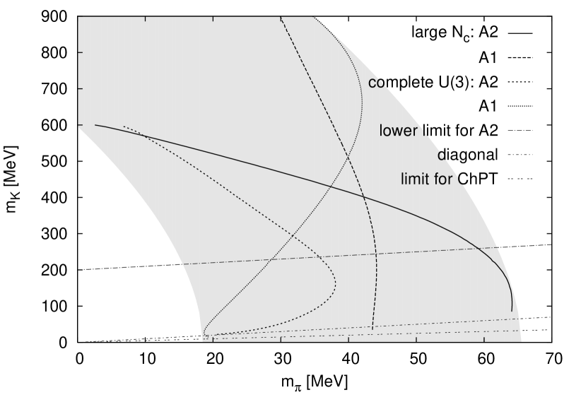
Figure 7: Phase boundary curves arising for $L\sigma M$ parametrizations compatible with $T=0$ ChPT. We present the boundary curves for alternatives ,A1’ and ,A2’ using the complete U(3) ChPT and the leading order large-$N_{c}$ ChPT at $\mathcal{O}(p^{2})$. The exact phase boundary curve is expected to lie in the light-grey shaded region. Crossover (first order transition) takes places at the right (left ) of the shaded region.

Figure 8: The temperature evolution of the nonstrange (x) and strange (y) condensates during a first order phase transition which takes place for $m_{\pi}=10$ MeV and $m_{K}=150$ MeV. The curves were obtained for alternative ,A1’ and the complete U(3) ChPT. Multivaluedness is observed in a given temperature range in both condensates.

Fig. 8 presents the phase diagram obtained in the case when all parameters are allowed to vary with $m_{\pi}$ and $m_{K}$. Due to the uncertainties in the scalar sector and also due to different approaches of the chiral perturbation theory (three-flavor or large-$N_{c}$) we can give only a band indicative of the theoretical uncertainties concerning the location of the real phase boundary of the model. Note, however, that all variants give a first order transition near the chiral limit, that is for small values of both the pion and kaon masses. We see, that for any value of $m_{K}\leq 800MeV$, the critical value of the pion mass does not exceed $65$ MeV. Our estimate for the phase boundary on the diagonal is $m_{\textrm{crit}}(\textrm{diag})=40\pm 20$ MeV. In the figure also the line is displayed below which we cannot trust the results of the alternative ,A2’, since its parameters diverge along the diagonal $m_{\pi}=m_{K}.$

First order transitions are signalled by multivaluedness in the temperature evolution of both the nonstrange and strange condensates, see Fig. 8. For large values of the kaon mass, we claim that the phase transition is driven by the variation of the nonstrange condensate, since the apparently different solutions of the strange condensate are very close to each other, and all stay at high values. Subsequent decrease of the strange condensate at higher temperature displays only a crossover. Along the phase boundary the critical temperature reaches $T_{c}\approx 170$ MeV near the physical kaon mass (in case ,A1’ and using large $N_{c}$ ChPT), then drops to $T_{c}=140$ MeV at both ends of the $m_{K}$ range shown in the figure, which is due to the effect of the chiral logarithms.

We could not provide evidence for a tricritical point on the $m_{\pi}=0$ axis for any of the alternatives ,A1’ and ,A2’. Alternative ,A1’ seems to predict it for such a high value of the kaon mass, where one can not trust ChPT, while ,A2’ does not work for $m_{\pi}=0$ because the solution of EoSs leaves the physical region.

Finally, we discuss a feature of our approximate solution in the low mass region which might be closely related to the problem of negative squared masses. It shows up the clearest along the diagonal, $m_{\pi}=m_{K}$, where the most plausible expectation would be to have a solution of EoS which satisfies, irrespective of the temperature, the condition $\sigma_{8}=0$. For the alternative ,A1’, (,A2’ does not work on the diagonal), it can be proved, using exclusively the tree–level stability criteria $3f_{1}+f_{2}>0$, that going towards the origin below a certain value of the Goldstone mass there is always a temperature range in which one of the squared mass eigenstates in the mixing scalar sector has negative eigenvalue. In this range we find in the physical region only solutions with $\sigma_{8}\neq 0$, that is the ’strange–nonstrange’ symmetry is apparently broken in an intermediate temperature range. It is not clear if this phase corresponds to the absolute minimum of the free energy. This solution is characterized by a large difference between the mass $m_{K}$ calculated from the second relation of Eq. (18) and the value of the pion mass, which is the largest one. In the mass region where both solutions (with $\sigma_{8}=0$ and $\sigma_{8}\neq 0$) exist the corresponding values of $\sigma_{0}$ are very close to each other. Therefore, we expect that even in the case where we cannot find the (true ?) minimum corresponding to $\sigma_{8}=0$, a good estimate of the position of the phase boundary on the diagonal is provided by the $\sigma_{8}\neq 0$ solution. The problem of negative squared masses shows up also in the $T=0$ finite quantum correction coming from the tadpole integrals, which were omitted in this work.

The above feature is a consequence of using tree–level expressions for the propagator masses. We certainly should have to go to higher–loop order in the resummed perturbation theory, also to take into account coupling resummations, for a complete resolution of the problem of negative mass squares including the assessment of the solution with $\sigma_{8}\neq 0$.

6 Conclusions

In this paper, we studied the phase boundary in the $(m_{\pi}-m_{K})$-plane allowing for the variation of all the parameters of the linear sigma model with $m_{\pi}$ and $m_{K}$. We used for this another low energy effective model, the chiral perturbation theory, which being a perturbative expansion in momenta and in quark masses about the chiral limit, provides, at each order of the momentum expansion, analytical relations displaying the dependence of the decay constants ($f_{\pi},f_{K}$) and masses of the $\eta$ and $\eta^{\prime}$ on the value of the pion and kaon masses. One could expect that the linear sigma model improved in this way will work reliably for small values of $m_{\pi}$ and $m_{K}$. Using accurate formulas to continue from the physical point, this approach could become an alternative to the lattice which has difficulties in exploring this region when information would be available on the variation of the mass of the $\sigma$ or $f_{0}$ scalar mesons in the ($m_{\pi}-m_{K})$-plane. The origin of the theoretical uncertainty of our findings is the lack of information on the scalar sector, which forces us to make assumptions. Lattice results about the mass dependence in the scalar sector would allow to reduce considerably the uncertainties of the parametrization of the model.

The model was solved using a mass ressumation in the framework of the optimized perturbation theory in order to resolve the negative squared mass problem of the perturbation theory in the broken symmetry phase. Unfortunately, resumming only one parameter, the mass, while respecting the Goldstone’s theorem for pions, violates Goldstone’s theorem for kaons. It also does not solve fully satisfactorily the problem of negative mass squares in the whole mass–plane, since the absolute minimum might be located in the $x-y$-plane slightly outside the physical domain. Resummation of another coupling is needed to fulfill all requirements imposed by Goldstone’s theorem. A possibility is to use the temperature variation of the coefficient of the $U_{A}(1)$ violating term $g$. Motivated by lattice studies this possibility was investigated in Costa .

Taking into account all theoretical uncertainties, we could estimate a band in the $(m_{\pi}-m_{K})$-plane for the phase boundary. Our estimate for the boundary point on the diagonal is $m_{\textrm{crit}}(\textrm{diag})=40\pm 20$ MeV, in nice agreement with the latest effective model and lattice studies.

Appendix A The $SU_{L}(3)~{}\times~{}SU_{R}(3)$ linear sigma model at tree–level

1.1 Mass eigenvalues, and mass matrices in the $0$-$8$ basis.

Using the inverse of the transformation (3), the mass matrix of $\eta$-s can be written in the more conventional $\eta_{0}$-$\eta_{8}$ basis:

$$m^{2}_{\eta_{00}} = \frac{1}{3}(2m^{2}_{\eta_{xx}}+m^{2}_{\eta_{yy}}+2\sqrt{2}\>m^{2}_{\eta_{xy}}),$$ (46)

$$m^{2}_{\eta_{88}} = \frac{1}{3}(2m^{2}_{\eta_{yy}}+m^{2}_{\eta_{xx}}-2\sqrt{2}\>m^{2}_{\eta_{xy}}),$$ (47)

$$m^{2}_{\eta_{08}} = \frac{1}{3}(\sqrt{2}(m^{2}_{\eta_{xx}}-m^{2}_{\eta_{yy}})-m^{2}_{\eta_{xy}}),$$ (48)

The mass eigenvalues and mixing angle $\theta_{\eta}$ are the following:

$$m^{2}_{\eta,\eta^{{}^{\prime}}}=\frac{1}{2}(m_{\eta_{00}}^{2}+m_{\eta_{88}}^{2}\mp\sqrt{(m_{\eta_{00}}^{2}-m_{\eta_{88}}^{2})^{2}+4m_{\eta_{08}}^{4}}),$$ (49)

$$\displaystyle\tan 2\theta_{\eta}=\frac{2m^{2}_{\eta_{08}}}{m^{2}_{\eta_{00}}-m^{2}_{\eta_{88}}},$$ (50)

where the ,-’ sign refers to $\eta$ and ,+’ refers to $\eta^{{}^{\prime}}$. These expressions hold also for the mixing in the scalar sector, where the lower mass eigenvalue is $m^{2}_{\sigma}$ and the higher is the squared mass of $f_{0}$.

1.2 The ,A2’ alternative

For the scalar octet, there is a GMO mass relation similar to the pseudoscalar sector, which to leading order reads:

$$4m^{2}_{\kappa}=m_{a_{0}}^{2}+3m^{2}_{\sigma_{88}}.$$ (51)

We characterize its accuracy by the following quantity:

$$r:=\left.\frac{4m^{2}_{\kappa}-m_{a_{0}}^{2}}{3m_{\sigma_{88}}^{2}}-1\right..$$ (52)

In the expression of $r$, the mass squares $m_{a_{0}}^{2}$ and $m^{2}_{\kappa}$ are determined by $f_{2},g,M^{2}$, which depend only on pseudoscalar mass squares: $m_{\pi}^{2}$, $m_{K}^{2}$, and $M_{\eta}^{2}=m_{\eta}^{2}+m_{\eta^{\prime}}^{2}$. In order to know $m_{\sigma_{88}}$, we should have $f_{1}$ and $\mu_{0}^{2}$ separately. For this purpose, in the physical point, we choose an $m_{\sigma}^{\textrm{ph}}$ to get $r^{\textrm{ph}}$. We require that the accuracy of scalar GMO to be independent of $m_{\pi}$, $m_{K}$, that is $r(m_{\pi},m_{K},m_{\sigma})=r(m_{\sigma}^{\textrm{ph}})=:r^{\textrm{ph}}$. After this, we can already determine $m_{\sigma_{88}}$ for arbitrary $m_{K}$, $m_{\pi}$ from (52), and we can split $M^{2}$ into $f_{1}$ and $\mu_{0}^{2}$. Using Table 1 and Eqs. (13)–(17) :

$$f_{1}^{(A2)} = \frac{m_{K}^{2}((-64f_{K}^{3}+104f_{\pi}f_{K}^{2}-58f_{\pi}^{2}f_{K}+9f_{\pi}^{3})r-12(2f_{K}-f_{\pi})(f_{K}-f_{\pi})^{2})}{32(3f_{\pi}^{2}-8f_{\pi}f_{K}+8f_{K}^{2})(f_{K}-f_{\pi})^{3}(r+1)}$$ (53)

$$+ \frac{m^{2}_{\pi}(r(16f_{\pi}^{3}+8f_{K}^{3}+24f_{\pi}f_{K}^{2}-39f_{\pi}^{2}f_{K})+4(f_{\pi}+2f_{K})(f_{K}-f_{\pi})^{2})}{32(3f_{\pi}^{2}-8f_{\pi}f_{K}+8f_{K}^{2})(f_{K}-f_{\pi})^{3}(r+1)}$$

$$+ \frac{M^{2}_{\eta}(f_{K}-f_{\pi})^{2}((2f_{K}-f_{\pi})r+f_{K}-f_{\pi})}{4(3f_{\pi}^{2}-8f_{\pi}f_{K}+8f_{K}^{2})(f_{K}-f_{\pi})^{3}(r+1)},$$

$${\mu_{0}^{2}}^{\,(A2)} = f_{1}^{(A2)}(6f_{\pi}^{2}-8f_{\pi}f_{K}+8f_{K}^{2})-{M^{2}},$$ (54)

where $r^{\textrm{ph}}\approx-0.017$, when $m_{\sigma}^{\textrm{ph}}=600$ MeV.

Appendix B The U(3) ChPT

The elements of the mass matrix of $\eta$-s are defined in (33):

$$m^{2}_{\eta_{88}} = D_{88}^{(0)}+d_{88}-(a_{88}D_{88}^{(0)}+a_{08}D_{08}^{(0)})\,,$$ (55)

$$m^{2}_{\eta_{00}} = D_{00}^{(0)}+d_{00}-(a_{00}D_{00}^{(0)}+a_{08}D_{08}^{(0)})\,,$$ (56)

$$m^{2}_{\eta_{08}} = D_{08}^{(0)}+d_{08}-\frac{1}{2}(a_{08}(D_{00}^{(0)}+D_{88}^{(0)})+D_{08}^{(0)}(a_{00}+a_{88}))\,,$$ (57)

together with the mixing angle defined in Eq. (50):

$$\tan 2\theta_{\eta}=\frac{2D_{08}^{(0)}}{D_{00}^{(0)}-D_{88}^{(0)}}\left[1-\frac{2d_{08}-a_{08}(D_{00}^{(0)}+D_{88}^{(0)})-D_{08}^{(0)}(a_{00}+a_{88})}{2D_{08}^{(0)}}+\frac{d_{00}-d_{88}-a_{00}D_{00}^{(0)}+a_{88}D_{88}^{(0)}}{D_{00}^{(0)}-D_{88}^{(0)}}\right]\,.$$ (58)

The relevant expressions of the $A$, $D$ matrices are given by Borasoy01 , Beisert01 :

$$\begin{aligned} a_{00}&=\frac{1}{f^{2}}\frac{2}{3}A(2+q)(3L_{4}+L_{5}),\\ a_{88}&=\frac{1}{f^{2}}(16A(2+q)L_{4}+\frac{16}{3}A(1+2q)L_{5}-2\mu_{K}),\\ a_{08}&=-\frac{16}{3\sqrt{2}}\frac{1}{f^{2}}A(q-1)L_{5},\end{aligned}\,\quad\begin{aligned} D_{00}^{(0)}&=-3v_{0}^{(2)}+\frac{2}{3}A(2+q),\\ D_{88}^{(0)}&=\frac{2}{3}A(1+2q),\\ D_{08}^{(0)}&=\frac{-2\sqrt{2}}{3}A(q-1),\end{aligned}$$ (59)

$$d_{88} =\frac{1}{f^{2}}\frac{2A}{9}\left[{96A}\left((2+q)^{2}L_{6}+2(q-1)^{2}L_{7}+(1+2q^{2})L_{8}\right)-(1+8q)\mu_{\eta}-9\mu_{\pi}+6\mu_{K}\right],$$ (60)

$$d_{00} =-4A(2+q)(v_{3}^{(1)}-3v_{2}^{(2)})$$

$$+\frac{1}{f^{2}}\frac{32A}{9}\left[A((2+q)^{2}(6L_{6}+2L_{7})+6(2+q^{2})L_{8})-\frac{1}{8}(\mu_{\pi}+6(1+q)\mu_{K}+(1+2q)\mu_{\eta})\right],$$

$$d_{08} =A(q-1)2\sqrt{2}v_{3}^{(1)}-\frac{1}{f^{2}}\frac{64\sqrt{2}}{3}A^{2}(q^{2}-1)L_{8}.$$

Therefore the elements of the mass matrix appearing in (55)–(57) are:

$$m^{2}_{\eta_{88}} = \frac{2}{3}A(1+2q)+\frac{A}{f^{2}}\left[\frac{32}{3}A(1+2q^{2})(2L_{8}-L_{5})-\frac{32}{3}A(1+2q)(2+q)L_{4}\right.{}$$ (61)

$$+ \left.\frac{128}{3}A(1-q)^{2}L_{7}+\frac{64}{3}A(2+q)^{2}L_{6}-\frac{2}{9}(1+8q)\mu_{\eta}-2\mu_{\pi}+\frac{8}{3}(1+q)\mu_{K}\right]$$

$$m^{2}_{\eta_{00}} = -3v_{0}^{(2)}+\frac{2}{3}A(2+q)\left[1-6v_{3}^{(1)}+18v_{2}^{(2)}+\frac{1}{f^{2}}\left(24v_{0}^{(2)}(3L_{4}+L_{5})\right)\right]{}$$ (62)

$$- \frac{A^{2}}{f^{2}}\left[\frac{16}{3}(2+q)^{2}(3L_{4}+L_{5}-6L_{6}-6L_{7})\right]{}$$

$$+ \frac{A}{f^{2}}\left[\frac{64}{9}A(3(2+q^{2})L_{8}-(1-q)^{2}L_{5})-\frac{4}{9}\mu_{\pi}+6(q+1)\mu_{K}+(2q+1)\mu_{\eta})\right]$$

$$m^{2}_{\eta_{08}} = \frac{-2\sqrt{2}}{3}A(q-1)\left[1-3v_{3}^{(1)}+\frac{1}{f^{2}}\left(12v_{0}^{(2)}L_{5}+16A(1+q)(2L_{8}-L_{5})-8A(2+q)L_{4}+\mu_{K}\right)\right].$$ (63)

Carefully substituting the ${\cal O}(1/f^{2})$ accurate expressions of $A$ and $q$ from (24), (25) into (61)-(63) we find for the variation of $m_{\eta_{00}}^{2},m_{\eta_{08}}^{2},m_{\eta_{88}}^{2}$ in the ($m_{\pi}-m_{K}$)–plane the following equations:

$$m_{\eta_{88}}^{2} = \frac{4m_{K}^{2}-m_{\pi}^{2}}{3}+\frac{1}{f^{2}}\left[\frac{8}{3}(\mu_{K}-\mu_{\eta})m_{K}^{2}+\frac{2}{3}(\mu_{\eta}-\mu_{\pi})m_{\pi}^{2}+\frac{32}{3}(2L_{8}-L_{5}+4L_{7})(m_{\pi}^{2}-m_{K}^{2})^{2}\right.{}$$ (64)

$$+ \left.\frac{32}{3}L_{6}(m_{\pi}^{4}-2m_{K}^{4}+m_{K}^{2}m_{\pi}^{2})\right],$$

$$m_{\eta_{00}}^{2} = -3v_{0}^{(2)}+\frac{2m_{K}^{2}+m_{\pi}^{2}}{3}\left(1-6v_{3}^{(1)}+18v_{2}^{(2)}+\frac{1}{f^{2}}24v_{0}^{(2)}(L_{5}+3L_{4})\right)+\frac{1}{f^{2}}\left[\frac{4}{3}(-2\mu_{K}-\mu_{\eta})m_{K}^{2}\right.$$ (65)

$$+ \left.\frac{1}{3}(\mu_{\eta}-7\mu_{\pi})m_{\pi}^{2}+\frac{16}{3}(2L_{8}-L_{5})(m_{\pi}^{2}-m_{K}^{2})^{2}+\frac{16}{3}L_{7}(m_{\pi}^{2}+2m_{K}^{2})^{2}\right],$$

$$m_{\eta_{08}}^{2} = \frac{2\sqrt{2}}{3}\left\{(m_{\pi}^{2}-m_{K}^{2})\left[1-3v_{3}^{(1)}+\frac{1}{f^{2}}\left(12v_{0}^{(2)}L_{5}-8(2L_{8}-L_{5})(m_{\pi}^{2}-m_{K}^{2})\right)\right]\right.$$ (66)

$$+ \left.\frac{1}{f^{2}}\left[4(L_{4}-4L_{6})(m_{\pi}^{4}+m_{K}^{2}m_{\pi}^{2}-2m_{K}^{4})+(\frac{1}{3}\mu_{\eta}-\mu_{\pi}+\mu_{K})m_{\pi}^{2}+(\frac{2}{3}\mu_{\eta}-\mu_{K})m_{K}^{2}\right]\right\}.$$

Appendix C The tadpole coefficients in EoS

Below we list the nonzero three-point couplings, needed for the evaluation of the tadpole contributions to EoS (see Eqs. (42), (43)) in the $x-y$ basis (4)

$$\begin{pmatrix}\alpha&\,t^{x}_{\alpha}&\,t^{y}_{\alpha}\\ \pi&\,2(2f_{1}+f_{2})x&\,4f_{1}y+g\\ K&\,2(2f_{1}+f_{2})x-f_{2}\sqrt{2}y+\frac{1}{\sqrt{2}}g&\,-f_{2}\sqrt{2}x+4(f_{1}+f_{2})y\\ \pi_{x}\pi_{x}&\,2(2f_{1}+f_{2})x&\,4f_{1}y-g\\ \pi_{y}\pi_{y}&\,4f_{1}x&\,4(f_{1}+f_{2})y\\ \pi_{x}\pi_{y}&\,-2g&\,0\\ a_{0}&\,2(2f_{1}+3f_{2})x&\,4f_{1}y-g\\ \kappa&\,2(2f_{1}+f_{2})x+f_{2}\sqrt{2}y-\frac{1}{\sqrt{2}}g&\,f_{2}\sqrt{2}x+4(f_{1}+f_{2})y\\ \sigma_{x}\sigma_{x}&\,6(2f_{1}+f_{2})x&\,4f_{1}y+g\\ \sigma_{y}\sigma_{y}&\,4f_{1}x&\,12(f_{1}+f_{2})y\\ \sigma_{x}\sigma_{y}&\,8f_{1}y+2g&\,8f_{1}x\\ \end{pmatrix}.$$ (67)

The tadpole integrals are evaluated in the mass eigenbasis, therefore in the pseudoscalar $x-y$ sector additional similarity transformations are needed in order to arrive at the coefficients of the $\eta,\eta^{\prime}$ tadpole integrals. The elements of the $2\times 2$ minor of $t^{x,y}$, which originally appears in the EoS, can be easily written in the mass eigenbasis. As an illustration we take the pseudoscalar $(\eta,\eta^{\prime})$ sector:

$$t_{xx}G_{xx}+t_{yy}G_{yy}+t_{xy}G_{xy}=\textnormal{Tr\,}\left[\begin{pmatrix}\displaystyle t_{xx}&\frac{t_{xy}}{2}\\ \frac{t_{xy}}{2}&t_{yy}\end{pmatrix}\begin{pmatrix}G_{xx}&G_{xy}\\ G_{xy}&G_{yy}\end{pmatrix}\right]=\textnormal{Tr\,}\left[R(\theta)\begin{pmatrix}\displaystyle t_{xx}&\frac{t_{xy}}{2}\\ \frac{t_{xy}}{2}&t_{yy}\end{pmatrix}R^{T}(\theta)\begin{pmatrix}G(m_{\eta^{\prime}})&0\\ 0&G(m_{\eta})\end{pmatrix}\right],$$

where $G_{xx}$ is the $xx$ element of the $2\times 2$ propagator matrix, $R(\theta)$ is an orthogonal transformation defined by $\tan 2\theta=2m^{2}_{\eta xy}/(m^{2}_{\eta xx}-m^{2}_{\eta yy})$ which relates the $x,y$ and $\eta^{\prime},\eta$ basis.

The diagonal $(\eta,\eta),(\eta^{\prime},\eta^{\prime})$ elements of the transformed matrix are the coefficients of the corresponding physical propagators and can be expressed as:

$$t_{\eta^{\prime},\eta}=\frac{1}{2}(t_{xx}+t_{yy})\pm\frac{(m^{2}_{\eta xx}-m^{2}_{\eta yy})(t_{xx}-t_{yy})+2m^{2}_{\eta xy}t_{xy}}{2\sqrt{\left(m^{2}_{\eta xx}-m^{2}_{\eta yy}\right)^{2}+4m^{4}_{\eta xy}}}.$$ (68)

References

- (1) for a recent review see, P. Petreczky, hep-lat/0409139 (to appear in Proc. of Lattice’04)
- (2) A. Barducci, R. Casalbuoni, G. Pettini and L. Ravagli, Phys. Rev. D 71, 016011 (2005)
- (3) D. Röder, J. Ruppert and D. H. Rischke, Phys. Rev. D 68, 016003 (2003)
- (4) J. B. Kogut and D. Toublan, Phys. Lett. B 564, 212 (2003)
- (5) L. He, P. Zhuang, Phys. Lett. B 615, 93 (2005)
- (6) R. D. Pisarski and F. Wilczek, Phys. Rev. D 29, R338 (1984)
- (7) F. Karsch, C. R. Allton, S. Ejiri, S. J. Hands, E. Laermann and C. Schmidt, Nucl. Phys. B (Proc. Suppl.) 129&130, 614 (2004), hep-lat/0309116
- (8) C. Bernard, T. Burch, C. deTar, S. Gottlieb, E. B. Gregory, U. M. Heller, J. Osborn, R. L. Sugar and D. Toussaint, hep-lat/0409097, (to appear in Procs. of Lattice’04)
- (9) S. Gavin, A. Gocksch and R.D. Pisarski, Phys. Rev. D 49, R3079 (1994)
- (10) Y. Hatta and T. Ikeda, Phys. Rev. D 67, 014028 (2003)
- (11) F. Karsch, E. Laermann and A. Peikert, Nucl. Phys. B605, 579 (2001)
- (12) H. Meyer-Ortmanns and B.J. Schaefer, Phys. Rev. D 53, 6586 (1996)
- (13) J.T. Lenaghan, D. H. Rischke and J. Schaffner-Bielich, Phys. Rev. D 62, 085008 (2000)
-
(14)
C. Schmidt,
PhD Thesis, Bielefeld University, 2003; result quoted in
karsch03 , available online at
ftp://ftp.uni-bielefeld.de/pub/papers/physik/theory/e6/dissertationen/schmidt.ps.gz - (15) J. T. Lenaghan, Phys. Rev. D 63, 037901 (2001)
- (16) J. M. Cornwall, R. Jackiw, and E. Tomboulis, Phys. Rev. D 10, 2428 (1974)
- (17) N. A. Törnqvist, Eur. Phys. J C 11, 359 (1999)
- (18) J. Gasser, H. Leutwyler, Nucl. Phys. B250, 465 (1985)
- (19) P. Herrera-Siklódy, J. I. Latorre, P. Pascual, J. Taron, Phys. Lett. B 419, 326 (1998)
- (20) P. Herrera-Siklódy, J. I. Latorre, P. Pascual, J. Taron, Nucl. Phys. B497, 345 (1997)
- (21) B. Borasoy, S. Wetzel, Phys. Rev. D 63, 074019 (2001)
- (22) N. Beisert, B. Borasoy, Eur. Phys. J. A 11, 329 (2001)
- (23) S. Chiku and T. Hatsuda, Phys. Rev. D 58, 076001 (1998)
- (24) L.-H. Chan and R. W. Haymaker, Phys. Rev. D 7, 402 (1973).
- (25) The 2004 Review of Particle Physics, S. Eidelman et al., Phys. Lett. B 592, 1 (2004)
- (26) KLOE Collaboration (A. Aloisio et al.): Phys. Lett. B 537, 21 (2002); E791 Collaboration (E. M. Aitala et al.): Phys. Rev. Lett. 86, 770 (2001)
- (27) D. B. Leinweber, A. W. Thomas, K. Tsushima, S. V. Wright, Phys. Rev. D 61, 074502 (2000); C. W. Bernard et al., Phys. Rev. D 64, 054506 (2001); S. Aoki et al., Phys. Rev. D 68, 054502 (2003)
- (28) M. Frink, U. G. Meißner, I. Scheller, hep-lat/0501024
- (29) A. Bramon, R. Escribano, J. L. L. Martínez, Phys. Rev. D 69, 074008 (2004)
- (30) A. Jakovác and Zs. Szép, Phys. Rev. D 71, 105001 (2005)
- (31) N. A. Törnqvist, in Proc. of IPN Orsay workshop “Chiral fluctuations in hadronic matter”, Eds. Z. Aouissat et al., p. 267, hep-ph/0201171
- (32) P. Costa, M. C. Ruivo, C. A. de Sousa and Yu. L. Kalinovsky, hep-ph/0502217 and hep-ph/0503258