STRONGLY AND WEAKLY UNSTABLE
ANISOTROPIC QUARK-GLUON PLASMA

Abstract

Using explicit solutions of the QCD transport equations, we derive an effective potential for an anisotropic quark-gluon plasma which under plausible assumptions holds beyond the Hard Loop approximation. The configurations, which are unstable in the linear response approach, are characterized by a negative quadratic term of the effective potential. The signs of higher order terms can be either negative or positive, depending on the parton momentum distribution. In the case of a Gaussian momentum distribution, the potential is negative and unbound from below. Therefore, the modes, which are unstable for gauge fields of small amplitude, remain unstable for arbitrary large amplitudes. We also present an example of a momentum distribution which gives a negative quadratic term of the effective potential but the whole potential has a minimum and it grows for sufficiently large gauge fields. Then, the system is weakly unstable. The character of the instability is important for the dynamical evolution of the plasma system.

I Introduction

An anisotropic quark-gluon plasma is unstable with respect to the transverse mode known as the filamentation or Weibel instability [1, 2, 3, 4, 5, 6]. The instabilities have recently focused some attention in the context of the phenomenology of nucleus-nucleus collisions at high energies. The experimental data on the particle spectra and the so-called elliptic flow, which have been obtained at the Relativistic Heavy-Ion Collider (RHIC) in Brookhaven National Laboratory, suggest, when analyzed within the hydrodynamical model, that an equilibration time of the parton system produced at the collision early stage is as short as 0.6 ${\rm fm}/c$ [7]. Calculations, which assume that the parton-parton collisions are responsible for the equilibration of the weakly interacting plasma, provide a significantly longer time of at least 2.6 ${\rm fm}/c$ [8]. To thermalize the system one needs either a few hard collisions of the momentum transfer of order of the characteristic parton momentum, which we denote here as $T$ (as the temperature of equilibrium system), or many collisions of smaller transfer. As discussed in e.g. [9], the time scale of the collisional equilibration is of order

$$t_{\rm hard}\sim\frac{1}{g^{4}{\rm ln}(1/g)\,T}\;,$$ (1)

where $g$ is the QCD coupling constant. The characteristic time of instability growth is roughly of order $1/gT$ for a sufficiently anisotropic momentum distribution [1, 4, 6, 10]. Therefore, the instabilities are much ‘faster’ than the hard collisions in the weak coupling regime. Since the system’s momentum distribution becomes more isotropic when the unstable modes develop, the instabilities have been argued [1, 10] to effectively speed up the thermalization processes. Very recent numerical simulation [11], where the fields, particles and color charges are treated classically, fully confirms the argument.

We note that the isotropization should be distinguished from the equilibration process[1]. The instabilities driven isotropization is a mean-field reversible phenomenon which is not associated with entropy production. Therefore, the collisions, which are responsible for the dissipation, are needed to reach the equilibrium state of maximal entropy. The instabilities contribute to the equilibration indirectly, reducing relative parton momenta and increasing the collision rate. And recently, it has been observed that the hydrodynamic collective behavior, which is evident in the experimental data [7], does not actually require local thermodynamic equilibrium but a merely isotropic momentum distribution of liquid components [10].

The stability analysis of the plasma system is usually performed within a linear response approach which assumes smallness of the gauge field amplitudes. An elegant qualitative argument [12] suggests that non-Abelian non-linearities do not stabilize the unstable modes as the system spontaneously chooses an Abelian configuration in the course of the instability development. This happens because the Abelian configuration corresponds to the steepest decrease of the effective Hard Loop potential. However, the phenomenon of abelianization which emerges from the numerical simulations [11, 12, 13, 14, 15] is more complex. In $1+1$ dimensions, i.e. when the gauge potentials depend on time and one space variable, the simulations [12, 13] of the Hard Loop anisotropic dynamics [16] and the classical simulation [11] show that initially the abelianization works well but it is less efficient when the fields become non-perturbatively large in the course of instability growth. The latter effect is nicely seen in the calculations [13]. In the simulations [14, 15] of the Hard Loop dynamics [16] performed in $1+3$ dimensions, the abelianization stops working at the non-perturbative scale and the growth of field amplitudes changes from exponential to linear.

The question arises what happens beyond the Hard Loop approximation, whether the higher-order non-linearites stop the instability growth, or maybe they make the system even more unstable. In attempt to address the question, we derive an effective potential of the plasma configuration which is known to be unstable at the Hard Loop level. We follow the method developed in our earlier paper [17] which uses explicit solutions of the QCD transport equations. To get the solutions, the system under study is assumed to be static and translation invariant in two space directions. The effective potential, which is obtained, thus corresponds to the simulations in $1+1$ dimensions. It holds at any order of the gauge coupling but a kind of Abelian approximation, which is justified due to the effect of abelianization, is needed to derive it. The higher order terms of the effective potential, which are relevant at sufficiently long times of instability development, carry information about the actual character of a plasma configuration. Depending of the momentum distribution of partons, the plasma is either weakly or strongly unstable.

Although we do not even attempt to solve the dynamical problem of temporal evolution of the unstable plasma – we merely derive the effective potential – we estimate various time scales of the instability growth. In particular, we show that the quartic and higher order terms of the potential become important at the same time scale when the fields starts to significantly influence the particle’s momenta, as explained in the concluding section.

Throughout the article we use the natural units with $\hbar=c=k_{\rm B}=1$. In Section II and in Appendix A, where we follow the four-dimensional notation, we use the metric convention $(1,-1,-1,-1)$ and we distinguish lower and upper Lorentz indices. In the remaining parts of the paper, where we mostly deal with three-vectors, all vectors are contravariant and to simplify the notation we do not longer distinguish lower and upper indices.

II The method

The distribution functions of quarks $(Q)$, antiquarks $(\bar{Q})$, and gluons $(G)$ are assumed to satisfy the collisionless transport equations

$$p^{\mu}D_{\mu}Q(p,x)+{g\over 2}\>p^{\mu}\left\{F_{\mu\nu}(x),{\partial Q(p,x)\over\partial p_{\nu}}\right\} = 0\;,$$ (3)

$$p^{\mu}D_{\mu}\bar{Q}(p,x)-{g\over 2}\>p^{\mu}\left\{F_{\mu\nu}(x),{\partial\bar{Q}(p,x)\over\partial p_{\nu}}\right\} = 0\;,$$ (4)

$$p^{\mu}{\cal D}_{\mu}G(p,x)+{g\over 2}\>p^{\mu}\left\{{\cal F}_{\mu\nu}(x),{\partial G(p,x)\over\partial p_{\nu}}\right\} = 0\;,$$ (5)

where $\{...,...\}$ denotes the anticommutator; the covariant derivatives $D_{\mu}$ and ${\cal D}_{\mu}$ act as

$$D_{\mu}=\partial_{\mu}-ig[A_{\mu}(x),...\;]\;,\;\;\;\;\;\;\;{\cal D}_{\mu}=\partial_{\mu}-ig[{\cal A}_{\mu}(x),...\;]\;,$$

$A_{\mu}$ and ${\cal A}_{\mu}$ being four-potentials in the fundamental and adjoint representations, respectively,

$$A^{\mu}(x)=A^{\mu}_{a}(x)\tau_{a}\;,\;\;\;\;\;{\cal A}^{\mu}_{ab}(x)=-if_{abc}A^{\mu}_{c}(x)\;,$$

and $f_{abc}$ are the structure constants of the ${\rm SU}(N_{c})$ group. Since the generators of ${\rm SU}(N_{c})$ in the adjoint representation are given by $(T_{a})_{bc}=-if_{abc}$, one can also write ${\cal A}^{\mu}=A^{\mu}_{a}T^{a}$. The field strength tensor in the fundamental representation is $F_{\mu\nu}=\partial_{\mu}A_{\nu}-\partial_{\nu}A_{\mu}-ig[A_{\mu},A_{\nu}]$, while ${\cal F}_{\mu\nu}$ denotes the strength tensor in the adjoint representation.

As already mentioned, the instability of interest is a very fast phenomenon. The characteristic time of instability development is not only much shorter than the characteristic time of hard parton-parton collisions (1) but it is also shorter than that of soft collisions which control the dissipation of the color degrees of freedom. In equilibrium, the collisions with momentum transfer of order $g^{2}T$ occur at the time scale [9]

$$t_{\rm soft}\sim\frac{1}{g^{2}{\rm ln}(1/g)\,T}\;.$$ (6)

Since the characteristic time of instability growth, which is roughly of order $1/gT$ for sufficiently anisotropic momentum distribution [1, 4, 6, 10], is much shorter than $t_{\rm soft}$, the collision terms of transport equations (II) can be neglected.

If a solution of the transport equations is known, one finds the associated color current which in the fundamental representation is

$$j^{\mu}(x)=-\frac{g}{2}\int dP\;p^{\mu}\Big{[}Q(p,x)-\bar{Q}(p,x)-{1\over N_{c}}{\rm Tr}\big{[}Q(p,x)-\bar{Q}(p,x)\big{]}+2i\tau_{a}f_{abc}G_{bc}(p,x)\Big{]}\;,$$ (7)

where the momentum measure

$$dP=\frac{d^{4}p}{(2\pi)^{3}}2\Theta(p_{0})\,\delta(p^{2})$$

takes into account the mass-shell condition $p_{0}=E_{p}=|{\bf p}|$. The adjoint currents equal $j^{\mu}_{a}(x)=2{\rm Tr}[\tau_{a}j^{\mu}(x)]$. Since the current is given by the relation

$$j_{a}^{\mu}(x)=-\frac{\delta S_{\rm eff}}{\delta A^{a}_{\mu}(x)}\;,$$ (8)

where $S_{\rm eff}\equiv\int d^{4}x\,{\cal L}_{\rm eff}\;$ is the effective action to be added to the Yang-Mills one, one obtains $S_{\rm eff}$ integrating Eq. (8).

Finding exact solutions of the transport equations (II) is in general a difficult task. However, it is possible to get such solutions under some restrictive conditions. Here we consider a system where both the gauge field and the distribution functions are invariant under some space-time translation(s), i.e.

$$\partial_{\alpha_{i}}A^{\mu}(x)=0\ ,\qquad\mu=0,1,2,3\ ,$$ (9)

and

$$\partial_{\alpha_{i}}Q(p,x)=\partial_{\alpha_{i}}\bar{Q}(p,x)=\partial_{\alpha_{i}}G(p,x)=0\;,$$ (10)

for a fixed $\alpha_{i}$, which can involve more than one Lorentz index. If $\alpha_{i}=0$ the system is static while for $\alpha_{i}=1,2,3$ the system is homogeneous - the gauge field and the distribution functions depend only on time.

We look for the solutions of the transport equations (II) in the form:

$$Q(p,x) = f(p_{\alpha_{i}}-gA_{\alpha_{i}}(x))=\sum_{n=0}^{\infty}\frac{(-g)^{n}}{n!}A_{\alpha_{1}}(x)\,A_{\alpha_{2}}(x)\cdots A_{\alpha_{n}}(x)\,\frac{\partial^{n}f(p_{\alpha_{i}})}{\partial p_{\alpha_{1}}\,\partial p_{\alpha_{2}}\ldots\,\partial p_{\alpha_{n}}}\;,$$ (12)

$$\bar{Q}(p,x) = \bar{f}(p_{\alpha_{i}}+gA_{\alpha_{i}}(x))=\sum_{n=0}^{\infty}\frac{g^{n}}{n!}A_{\alpha_{1}}(x)\,A_{\alpha_{2}}(x)\cdots A_{\alpha_{n}}(x)\,\frac{\partial^{n}\bar{f}(p_{\alpha_{i}})}{\partial p_{\alpha_{1}}\,\partial p_{\alpha_{2}}\ldots\partial p_{\alpha_{n}}}\;,$$ (13)

$$G(p,x) = f_{g}(p_{\alpha_{i}}-g{\cal A}_{\alpha_{i}}(x))=\sum_{n=0}^{\infty}\frac{(-g)^{n}}{n!}{\cal A}_{\alpha_{1}}(x)\,{\cal A}_{\alpha_{2}}(x)\cdots{\cal A}_{\alpha_{n}}(x)\,\frac{\partial^{n}f_{g}(p_{\alpha_{i}})}{\partial p_{\alpha_{1}}\,\partial p_{\alpha_{2}}\ldots\partial p_{\alpha_{n}}}\;,$$ (14)

where it is understood that a sum is taken over the repeated indices. The functions $f$, $\bar{f}$ and $f_{g}$ are, in principle, arbitrary but they can be fixed by additional considerations. The solutions of the form (II) do not assume smallness of $gA$ provided the series (II) are not terminated at a finite number of terms. We stress that all components of the four-vector $p^{\mu}$ are treated here as independent variables.

One finds that the expressions (II) exactly solve Eqs. (II) when

$$[D_{\mu}A_{\alpha_{i}},A_{\alpha_{j}}]=0\ ,\qquad\mu=0,1,2,3\;,$$ (15)

and

$$[{\cal D}_{\mu}{\cal A}_{\alpha_{i}},{\cal A}_{\alpha_{j}}]=0\,\qquad\mu=0,1,2,3\;.$$ (16)

We note that Eq. (16) is automatically satisfied if Eq. (15) holds. The condition (15) is satisfied when, in particular, $A^{\mu}_{a}$ has only non-vanishing components in the Cartan subalgebra of ${\rm SU}(N_{c})$ which for ${\rm SU}(3)$ are in the $a=3,8$ directions of the color space. If $A^{\mu}_{a}$ has only one color component, the condition (15) is also trivially satisfied.

Having solutions of the transport equations, one finds the associated color current. Inserting the expressions (II) into Eq. (7), one gets

$$j_{a}^{\mu}(x) = \sum_{n=0}^{\infty}\frac{(-g)^{n+1}}{n!}A_{\alpha_{1}}^{c_{1}}(x)\cdots A_{\alpha_{n}}^{c_{n}}(x)\int dP\;p^{\mu}$$ (17)

$$\times \bigg{\{}{\rm Tr}[\tau_{a}\tau_{c_{1}}\cdots\tau_{c_{n}}]\bigg{[}\frac{\partial^{n}f(p_{\alpha_{i}})}{\partial p_{\alpha_{1}}\cdots\,\partial p_{\alpha_{n}}}+(-1)^{n+1}\frac{\partial^{n}{\bar{f}}(p_{\alpha_{i}})}{\partial p_{\alpha_{1}}\cdots\,\partial p_{\alpha_{n}}}\bigg{]}+{\rm Tr}[T_{a}T_{c_{1}}\cdots T_{c_{n}}]\frac{\partial^{n}f_{g}(p_{\alpha_{i}})}{\partial p_{\alpha_{1}}\cdots\,\partial p_{\alpha_{n}}}\bigg{\}}\;.$$ (18)

The current (17) provides, after integrating Eq. (8), the effective lagrangian of the form [17]

$${\cal L}_{\rm eff}=-\sum_{n=0}^{\infty}\frac{(-g)^{n+1}}{(n+1)!} \bigg{\{} {\rm Tr}[A_{\alpha_{1}}(x)\cdots A_{\alpha_{n+1}}(x)]\int dP\>p^{\alpha_{1}}\>\bigg{[}\frac{\partial^{n}f(p_{\alpha_{i}})}{\partial p_{\alpha_{2}}\cdots\,\partial p_{\alpha_{n+1}}}+(-1)^{n+1}\frac{\partial^{n}{\bar{f}}(p_{\alpha_{i}})}{\partial p_{\alpha_{1}}\cdots\,\partial p_{\alpha_{n}}}\bigg{]}$$ (19)

$$+ {\rm Tr}[{\cal A}_{\alpha_{1}}(x)\cdots{\cal A}_{\alpha_{n+1}}(x)]\int dP\>p^{\alpha_{1}}\>\frac{\partial^{n}f_{g}(p_{\alpha_{i}})}{\partial p_{\alpha_{2}}\cdots\,\partial p_{\alpha_{n+1}}}\bigg{\}}\;.$$ (20)

The distribution functions $f$, $\bar{f}$ and $f_{g}$ include two helicity states of, respectively, quarks, antiquarks and gluons. Various quark flavour states are also included in $f$ and $\bar{f}$. We note that Eq. (20) with the equilibrium distribution functions provides in the static case ($\alpha_{i}=0$) the full one-loop effective potential [17].

To get the complete action, the lagrangian (20) should be supplemented by the gauge field ‘kinetic’ term $-\frac{1}{4}F^{a}_{\mu\nu}F^{a\mu\nu}$ which involves, due to its non-Abelian nature, not only quadratic but also cubic and quartic terms of the potential $A^{\mu}_{a}$. Since the lagrangian (20) has been derived under the assumption that the gauge fields obey the condition (15), the same condition must be applied to the ‘kinetic’ term, which then becomes effectively Abelian.

As seen, the effective lagrangian (19) is local. In general, this as a consequence of the space-time homogeneity (9,10) combined with the commutation condition (15). However, it should be stressed that, as explicitly shown in [17], the $g^{2}$ term of the lagrangian (19) does not require the condition (15) which is needed for the higher order terms. The quadratic term and its relationship to the potential obtained within the linear response method is further discussed in Appendix A.

The Hard Loop action can be found for both the equilibrium [18, 19, 20, 21] and anisotropic [16] plasmas, modifying the $g^{2}$ term of the lagrangian (19) to comply with gauge invariance. Presumably, the higher order terms of the effective potential (19) can be also generalized in the same way, once the space-time invariance is abandoned. However, we are not going to follow this direction. Our purpose here is to understand the possible role of the higher order terms of Eq. (19), whose coefficients are uniquely fixed by powers of $g$ and by the parton distribution functions.

III Effective potential for unstable configurations

In this section we discuss configurations which are known to be unstable in the linear response approach. Specifically, we consider the filamentation instability which occurs in the homogeneous plasma when the momentum distribution is anisotropic. When the instability develops, the kinetic energy of particles is converted into field energy. The wave vector of the unstable mode is perpendicular to the direction with a ‘surplus’ of the momentum and it points towards the direction with the momentum ‘deficit’. We choose the wave vector along the $z$ axis and we expect to observe an instability when the momentum distribution is elongated in the $x$ or $y$ direction when compared to the momentum in the $z$ direction. In Sec. II we have carefully distinguished the upper and lower indices of four-vectors. From now on, all four-vectors are contravariant and the upper and lower indices are no longer distinguished (except the Yang-Mills lagrangian written in a relativistically covariant form).

Let us now consider a geometry of the filamentation instability referring to classical electrodynamics [2]. Due to the ‘surplus’ of momentum along the $x$ or $y$ axis, the fluctuations of current flowing in the $x\!-\!y$ plane are amplified. Thus, we expect non-vanishing $x$ or/and $y$ current components. When the wave vector of a standing (time independent) wave points in the $z$ direction (${\bf k}=(0,0,k)$) and the current (${\bf j}$) flows in the $x\!-\!y$ plane, there are non-vanishing $x$ and $y$ components of the vector potential (${\bf A}$) and the magnetic field (${\bf B}$). Indeed, one checks that

$${\bf j}=(a_{x}k^{2}{\rm sin}(kz),a_{y}k^{2}{\rm sin}(kz),0)\;,\;\;\;\;\;\;\;{\bf A}=(a_{x}{\rm sin}(kz),a_{y}{\rm sin}(kz),0)\;,\;\;\;\;\;\;\;{\bf B}=(-a_{y}k\,{\rm cos}(kz),a_{x}k\,{\rm cos}(kz),0)\;,$$ (21)

which depend only on $z$, satisfy the electromagnetic equations

$$\nabla\times{\bf B}={\bf j}\;,\;\;\;\;\;\;\;\nabla\times{\bf A}={\bf B}\;.$$ (22)

As seen, the dynamics of the system, which is static and invariant with respect to the translations in $x$ and $y$ directions, can be still nontrivial. Therefore, we consider such a quark-gluon system. The solution of the transport equation is then of the form $f(p_{0}-gA_{0}(z),p_{x}-gA_{x}(z),p_{y}-gA_{y}(z))$. Since the filamentation mode is transverse and the magnetic field is responsible for the instability development, we can choose the gauge condition $A_{0}=0$. Finally, the distribution function is assumed to obey the mirror symmetry

$$f(p_{0},{\bf p})=f(p_{0},-{\bf p})\;.$$ (23)

Then, the formula (20) for $\alpha_{i}=x,y$ gives the effective potential $V_{\rm eff}\equiv-{\cal L}_{\rm eff}$ as

$$V_{\rm eff} = -\frac{g^{2}}{2!}\Big{\{}\Big{\langle}\frac{p_{x}}{p_{0}}\frac{\partial}{\partial p_{x}}\Big{\rangle}\,{\rm Tr}[A_{x}^{2}]+\Big{\langle}\frac{p_{y}}{p_{0}}\frac{\partial}{\partial p_{y}}\Big{\rangle}\,{\rm Tr}[A_{y}^{2}]\Big{\}}$$ (24)

$$- \frac{g^{4}}{4!}\Big{\{}\Big{\langle}\frac{p_{x}}{p_{0}}\frac{\partial^{3}}{\partial p^{3}_{x}}\Big{\rangle}\,{\rm Tr}[A_{x}^{4}]+\Big{\langle}\frac{p_{y}}{p_{0}}\frac{\partial^{3}}{\partial p^{3}_{y}}\Big{\rangle}\,{\rm Tr}[A_{y}^{4}]+3\Big{(}\Big{\langle}\frac{p_{y}}{p_{0}}\frac{\partial^{3}}{\partial p^{2}_{x}\partial p_{y}}\Big{\rangle}+\Big{\langle}\frac{p_{x}}{p_{0}}\frac{\partial^{3}}{\partial p^{2}_{y}\partial p_{x}}\Big{\rangle}\Big{)}\,{\rm Tr}[A_{x}^{2}A_{y}^{2}]\Big{\}}+{\cal O}(g^{6})\;,$$ (25)

where

$$\langle\cdots\rangle\equiv\int dP\,p^{0}\;\cdots f(p)\;.$$ (26)

If the quantity, which is averaged over four-momenta, is independent of $p_{0}$, the integration over $p_{0}$ is performed and

$$\langle\cdots\rangle=\int\frac{d^{3}p}{(2\pi)^{3}}\cdots f({\bf p})\;.$$

The function $f({\bf p})$ should be understood as $f(E_{p},{\bf p})$. We note that only the quark contribution is taken into account in Eq. (24). Including the contributions of antiquarks and gluons is straightforward. We also observe that due to the mirror symmetry condition (23), there are only terms of even powers of $A$ in Eq. (24).

To study the system’s stability, the effective potential generated by the quasiparticles should be supplemented by a potential-like contribution coming from the Yang-Mills ‘kinetic’ contribution to the lagrangian $-\frac{1}{4}F^{a}_{\mu\nu}F^{a\,\mu\nu}$. Since we consider static configurations in the $A^{0}=0$ gauge, the lagrangian equals

$$-\frac{1}{4}F^{a}_{\mu\nu}F^{a\,\mu\nu}=-\frac{1}{2}{\bf B}^{a}{\bf B}^{a}\;,$$

where the chromomagnetic field ${\bf B}^{a}$ is defined as

$${\bf B}^{a}\equiv\nabla\times{\bf A}^{a}+\frac{g}{2}f^{abc}{\bf A}^{b}\times{\bf A}^{c}\;.$$

The Yang-Mills lagrangian is built of the gauge potentials and their gradients. We identify as a contribution to the effective potential the term of the Yang-Mills lagrangian where gradients of ${\bf A}^{a}$ are absent. This is the only term which survives in a homogeneous system, and it reads

$$V_{\rm YM}=\frac{1}{4}g^{2}f^{abc}f^{ade}({\bf A}^{b}{\bf A}^{d})({\bf A}^{c}{\bf A}^{e})\;.$$ (27)

Because of this term, the system has been argued [12] to spontaneously choose an Abelian configuration in the course of the instability development. We will assume that this is the case, thus justifying the Abelian-like conditions (9) under which the effective Lagrangian (19) was obtained. As noted in the Introduction, the simulations in $1+1$ dimensions [11, 12, 13], which are relevant for our study, confirm effectiveness of the abelianization. We return to this problem in the concluding section.

The negative sign of the quadratic term of the potential (24) usually signals the instability. Let us consider the issue. Within the linear response analysis, unstable modes are found, see e.g. [22], as solutions of the dispersion equation

$${\rm det}[{\bf k}^{2}\delta^{ij}-k^{i}k^{j}-\omega^{2}-\Pi^{ij}(\omega,{\bf k})]=0\;.$$

The polarization tensor of anisotropic plasma, which was derived in [22], is given in Appendix A by Eq. (A4).

Further, we consider a simplified situation where the wave vector points in the $z$ direction (${\bf k}=(0,0,k)$) and the chromoelectromagnetic field has only one non-vanishing component along the $x$ axis. Then, as discussed in e.g. [3], the dispersion equation for the mirror symmetric momentum distribution simplifies to

$$k^{2}-\omega^{2}-\Pi^{xx}(\omega,k)=0\;.$$ (28)

The unstable modes of interest correspond to the solutions of Eq. (28) with positive imaginary frequency. The existence of unstable modes is controlled by the so-called Penrose criterion [23], which was applied to the simplified equation (28) in [1] while a general configuration was studied in [6]. According to the Penrose criterion, there are unstable solutions of Eq. (28) if there are such wave vectors $k$ that

$$k^{2}-\Pi^{xx}(\omega=0,k)<0\;.$$ (29)

Since $\Pi^{xx}(\omega=0,k)$, as given by Eq. (A4), is independent of $k$, the Penrose criterion (29) reads

$$\int dP\>p_{x}\bigg{[}\frac{\partial f}{\partial p_{x}}-\frac{p_{x}}{p_{z}}\frac{\partial f}{\partial p_{z}}\bigg{]}>0\;.$$ (30)

The respective quadratic term of the effective potential (24) is negative when

$$\int dP\>p_{x}\frac{\partial f}{\partial p_{x}}>0\;.$$ (31)

The criteria (30, 31) appear to be fully equivalent to each other. Since the system under consideration is static and translationally invariant along the $x$ and $y$ directions, the solutions of the transport equations cannot explicitly depend on $p_{z}$. Therefore, the last term in Eq. (30) vanishes identically.

Essential information contained in the potential (24) is carried by the sign of each term. As discussed above, the negative sign of the quadratic term signals instability of small amplitude modes. Depending on signs of higher order terms, one deals with strongly unstable or weakly unstable configurations. In the next sections we consider examples of momentum distributions which illustrate the two situations.

IV Strongly unstable configuration

We consider here a specific Gaussian form of the distribution function $f$. Namely, the function is chosen as

$$f(p_{x},p_{y},p_{0})=2^{3}\pi^{3/2}\sqrt{\beta(\beta-\alpha_{x})(\beta-\alpha_{y})}\,\rho\,{\rm exp}\Big{(}\alpha_{x}p_{x}^{2}+\alpha_{y}p_{y}^{2}-\beta\,p_{0}^{2}\Big{)}\;,$$ (32)

where $\rho$ is the quark density ($\rho=\langle 1\rangle$) while the parameters $\alpha_{x}$, $\alpha_{y}$ and $\beta$ ($\beta>0\,,\;\beta>\alpha_{x}\,,\;\beta>\alpha_{y}$) control the momentum distribution. One observes that taking into account the mass-shell constraint $p_{0}=E_{p}=\sqrt{p_{x}^{2}+p_{y}^{2}+p_{z}^{2}}$, the distribution function equals

$$f(p_{x},p_{y},E_{p})=2^{3}\pi^{3/2}\sqrt{\beta(\beta-\alpha_{x})(\beta-\alpha_{y})}\,\rho\,{\rm exp}\Big{(}-(\beta-\alpha_{x})p_{x}^{2}-(\beta-\alpha_{y})p^{2}_{y}-\beta p_{z}^{2}\Big{)}\;,$$ (33)

and one immediately finds

$$\langle p_{x}^{2}\rangle=\frac{\rho}{2(\beta-\alpha_{x})}\;,\;\;\;\;\;\;\;\langle p_{y}^{2}\rangle=\frac{\rho}{2(\beta-\alpha_{y})}\;,\;\;\;\;\;\;\;\langle p_{z}^{2}\rangle=\frac{\rho}{2\beta}\;.$$

With the distribution function (32), the momentum derivatives in Eq. (24) are trivially computed and the effective potential reads

$$V_{\rm eff} = -g^{2}\Big{\{}\alpha_{x}\Big{\langle}\frac{p_{x}^{2}}{E_{p}}\Big{\rangle}\,{\rm Tr}[A_{x}^{2}]+\alpha_{y}\Big{\langle}\frac{p_{y}^{2}}{E_{p}}\Big{\rangle}\,{\rm Tr}[A_{y}^{2}]\Big{\}}$$ (36)

$$-g^{4}\bigg{\{}\Big{(}\frac{1}{3}\alpha_{x}^{3}\Big{\langle}\frac{p_{x}^{4}}{E_{p}}\Big{\rangle}+\frac{1}{2}\alpha_{x}^{2}\Big{\langle}\frac{p_{x}^{2}}{E_{p}}\Big{\rangle}\Big{)}\,{\rm Tr}[A_{x}^{4}]+\Big{(}\frac{1}{3}\alpha_{y}^{3}\Big{\langle}\frac{p_{y}^{4}}{E_{p}}\Big{\rangle}+\frac{1}{2}\alpha_{y}^{2}\Big{\langle}\frac{p_{y}^{2}}{E_{p}}\Big{\rangle}\Big{)}\,{\rm Tr}[A_{y}^{4}]$$

$$\;\;\;\;\;\;+\Big{(}(\alpha_{x}\alpha_{y}^{2}+\alpha_{x}^{2}\alpha_{y})\Big{\langle}\frac{p_{x}^{2}p_{y}^{2}}{E_{p}}\Big{\rangle}+\frac{1}{2}\alpha_{x}\alpha_{y}\Big{\langle}\frac{p_{x}^{2}+p_{y}^{2}}{E_{p}}\Big{\rangle}\Big{)}\,{\rm Tr}[A_{x}^{2}A_{y}^{2}]\bigg{\}}+{\cal O}(g^{6})\;.$$

The terms of higher powers of $g$, which are suppressed in the small coupling regime, can be easily calculated as well. The moments of the Gaussian distribution function can be computed analytically and expressed through hypergeometric functions but the results are of rather complicated form, and thus they are not very useful. We observe that the moments of the Gaussian distribution function, which are present in Eq. (36), are all positive. Therefore, the potential (36) is negative when $\alpha_{x}$ and $\alpha_{y}$ are positive. We note that the higher order terms are also negative for $\alpha_{x}>0$ and $\alpha_{y}>0$. Then, the effective potential is negative and unbound from below for an arbitrary magnitude of the gauge potential. We also observe that the infinite series with the first few terms given by Eq. (36) is convergent for any value of the gauge potential as the Gaussian function is regular and its derivatives of any order are finite.

Obviously, the gauge field amplitude cannot roll down to infinity, as suggests the potential (36), and there are several dynamical processes that can stop the field growth, rebuilding the effective potential. We keep in mind here the non-Abelian non-linearities, isotropization, equilibration which operate at different time scales briefly discussed in the concluding section. Quantitative analysis of these effects requires a dynamic treatment which includes the back reaction and self-consistent generation of fields. We only mention here that if no other processes stop the instability development, the inter-parton collisions will certainly do the job. The collisions, which are neglected in our analysis, slowly drive the system towards equilibrium. And when the thermodynamic equilibrium is reached, the system is no longer unstable - the effective potential becomes positive with a minimum corresponding the equilibrium configuration.

Below we consider two special cases of the distribution function (32) which are of interest in the context of phenomenology of heavy-ion collisions. When two relativistic nuclei of equal mass collide, the parton momentum distribution in the center of mass frame is initially elongated along the beam axis - it corresponds to a prolate ellipsoid. With the time passing, the parton momentum distribution in the local rest frame evolves due to the parton free streaming towards an oblate shape with the momentum squeezed along the beam direction. The two configurations are discussed below.

A Prolate shape

When $\alpha_{y}=0$ and $\alpha_{\parallel}\equiv\alpha_{x}$, the momentum distribution (33) is

$$f(p_{x},p_{y},E_{p})=2^{3}\pi^{3/2}\beta\sqrt{\beta-\alpha_{\parallel}}\,\rho\,{\rm exp}\Big{(}-(\beta-\alpha_{\parallel})p_{x}^{2}-\beta(p^{2}_{y}+p_{z}^{2})\Big{)}\;,$$ (37)

where, as previously, $\alpha_{\parallel}<\beta$ and $\beta>0$, and

$$\langle p_{x}^{2}\rangle=\frac{\rho}{2(\beta-\alpha_{\parallel})}\;,\;\;\;\;\;\;\;\langle p_{y}^{2}\rangle=\langle p_{z}^{2}\rangle=\frac{\rho}{2\beta}\;.$$

For $\alpha_{\parallel}>0$ the distribution (37) corresponds to the prolate ellipsoid elongated along the $x$ axis. The effective potential (36) for the distribution (37) equals

$$V_{\rm eff}=-g^{2}\alpha_{\parallel}\Big{\langle}\frac{p_{x}^{2}}{E_{p}}\Big{\rangle}\,{\rm Tr}[A_{x}^{2}]-g^{4}\Big{(}\frac{1}{3}\alpha_{\parallel}^{3}\Big{\langle}\frac{p_{x}^{4}}{E_{p}}\Big{\rangle}+\frac{1}{2}\alpha_{\parallel}^{2}\Big{\langle}\frac{p_{x}^{2}}{E_{p}}\Big{\rangle}\Big{)}\,{\rm Tr}[A_{x}^{4}]+{\cal O}(g^{6})\;.$$ (38)

One observes that when the momentum ellipsoid is elongated in the $x$ direction ($\alpha_{\parallel}>0$), the potential (38) is negative and unbound from below.

B Oblate shape

When $\alpha_{\perp}\equiv\alpha_{x}=\alpha_{y}$, the momentum distribution (33) is

$$f(p_{x},p_{y},E_{p})=2^{3}\pi^{3/2}\sqrt{\beta}(\beta-\alpha_{\perp})\,\rho\,{\rm exp}\Big{(}-(\beta-\alpha_{\perp})p_{\perp}^{2}-\beta p_{z}^{2}\Big{)}\;,$$ (39)

where $\alpha_{\perp}<\beta$, $\beta>0$ and $p_{\perp}^{2}\equiv p_{x}^{2}+p_{y}^{2}$. One observes that

$$\langle p_{x}^{2}\rangle=\langle p_{y}^{2}\rangle=\frac{1}{2}\langle p_{\perp}^{2}\rangle=\frac{\rho}{2(\beta-\alpha_{\perp})}\;,\;\;\;\;\;\;\;\langle p_{z}^{2}\rangle=\frac{\rho}{2\beta}\;.$$

For $\alpha_{\perp}>0$ the distribution (39) corresponds to the oblate ellipsoid squeezed along the $z$ axis. The effective potential (36) for the momentum distribution (39) equals

$$V_{\rm eff} = -\frac{1}{2}g^{2}\alpha_{\perp}\Big{\langle}\frac{p_{\perp}^{2}}{E_{p}}\Big{\rangle}\,{\rm Tr}[A_{x}^{2}+A_{y}^{2}]$$ (41)

$$-g^{4}\bigg{\{}\Big{(}\frac{1}{8}\alpha_{\perp}^{3}\Big{\langle}\frac{p_{\perp}^{4}}{E_{p}}\Big{\rangle}+\frac{1}{4}\alpha_{\perp}^{2}\Big{\langle}\frac{p_{\perp}^{2}}{E_{p}}\Big{\rangle}\Big{)}\,{\rm Tr}[A_{x}^{4}+A_{y}^{4}]+\Big{(}\frac{1}{4}\alpha_{\perp}^{3}\Big{\langle}\frac{p_{\perp}^{4}}{E_{p}}\Big{\rangle}+\frac{1}{2}\alpha_{\perp}^{2}\Big{\langle}\frac{p_{\perp}^{2}}{E_{p}}\Big{\rangle}\Big{)}\,{\rm Tr}[A_{x}^{2}A_{y}^{2}]\bigg{\}}+{\cal O}(g^{6})\;.$$

When the momentum ellipsoid is squeezed in the $z$ direction ($\alpha_{\perp}>0$), the potential (41) is negative and unbound from below - all terms are negative.

V Weakly unstable configuration

The effective potential crucially depends on the parton momentum distribution. The Gaussian distribution discussed in the previous section provides an effective potential where the quartic and higher order terms are negative once the quadratic term is negative. In such a case, a mode, which is unstable in the linear response approach, remains unstable for gauge fields of larger amplitude. However, it is not difficult to invent a momentum distribution which gives a negative quadratic term of the effective potential and a positive quartic term. Then, an unstable mode in the linear response approximation is stabilized when the field’s amplitude becomes sufficiently large.

As previously, we consider here a static system which is homogeneous along the $x$ and $y$ directions and we choose the momentum distribution of the form

$$f(p_{x},p_{y},p_{0})=\frac{2\pi^{2}\beta^{2}}{1+\beta{\cal P}}\,e^{\beta{\cal P}}\,\rho\,\big{[}\delta(p_{x}-{\cal P})+\delta(p_{x}+{\cal P})\big{]}\,e^{-\beta p_{0}}\;,$$ (42)

with $\beta>0$ and ${\cal P}>0$. As in the case of the Gaussian distribution, the normalizing constant is chosen in such a way that the quark density $\rho$ equals $\langle 1\rangle$. The computation of the constant is explained in Appendix B. The distribution (42) describes two counter-streaming beams of quarks with the momenta $p_{x}={\cal P}$ and $p_{x}=-{\cal P}$. The momentum in the $y\!-\!z$ plane is distributed according to $\sim{\rm exp}\Big{(}-\beta\sqrt{{\cal P}^{2}+p_{y}^{2}+p_{z}^{2}}\Big{)}$.

The effective potential (24) computed with the distribution (42) equals

$$V_{\rm eff}=\frac{g^{2}}{2!}\rho\,\beta\,\frac{1-\beta{\cal P}}{1+\beta{\cal P}}\,{\rm Tr}[A_{x}^{2}] + \frac{g^{4}}{4!}\rho\,\beta^{3}\,\frac{3-\beta{\cal P}}{1+\beta{\cal P}}\,{\rm Tr}[A_{x}^{4}]$$ (43)

$$+ \cdots+\frac{g^{2n}}{(2n)!}\rho\,\beta^{2n-1}\,\frac{2n-1-\beta{\cal P}}{1+\beta{\cal P}}\,{\rm Tr}[A_{x}^{2n}]+\cdots$$ (44)

The calculation details are given in Appendix B. As seen, for $1/\beta<{\cal P}<3/\beta$ the quadratic term is negative but the quartic and higher term are positive. Then, the mode, which is unstable in the linear response approximation, is stabilized when the field’s amplitude becomes so large that the quartic term matters.

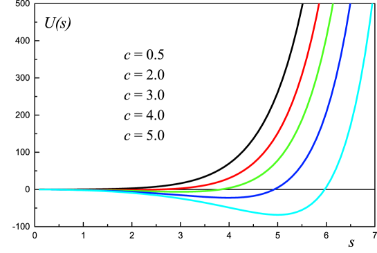
FIG. 1.: The effective potential (46) for 5 values of the parameter $c$. The most upper line corresponds to $c=0.5$, the lower one to $c=2.0$, etc.

Interestingly, the series (44) can be summed up and the result is

$$V_{\rm eff}=\frac{\rho}{\beta(1+\beta{\cal P})}\,{\rm Tr}\big{[}-\beta{\cal P}\,\big{(}{\rm ch}(\beta gA_{x})-1\big{)}+\beta gA_{x}{\rm sh}(\beta gA_{x})-{\rm ch}(\beta gA_{x})+1\big{]}\;.$$ (45)

To further analyze the effective potential (45), we define the dimensionless potential $U\equiv\beta(1+\beta{\cal P})V_{\rm eff}/\rho$ , the dimensionless parameter $c\equiv\beta{\cal P}>0$ and the dimensionless variable $s\equiv\beta gA_{x}$. The gauge potential $A_{x}$ is treated as a scalar, not matrix, quantity. Then,

$$U(s)=(1+c)(1-{\rm ch}s)+s\,{\rm sh}s\;.$$ (46)

One easily finds

$$U(s)\approx\left\{\begin{array}[]{ccc}\frac{1-c}{2}\,s^{2}+\frac{3-c}{24}\,s^{4}&{\rm for}&\frac{1}{s}\gg 1\;,\\[8.53581pt] \frac{s-c}{2}\,e^{s}&{\rm for}&s\gg 1\;.\end{array}\right.$$

As seen, the potential $U(s)$ always grows for sufficiently large $s$. Since the derivative of $U(s)$ equals $U^{\prime}(s)=-c\,{\rm sh}s+s\,{\rm ch}s$, the potential $U(s)$ monotonously grows for $c<1$ as the equation $s=c\,{\rm th}s$ has no solution. For $c>1$ the potential has a minimum. For $c$ only slightly exceeding unity i.e. such that $0<c-1\ll 1$, the potential is minimized for $s_{\rm min}\approx\sqrt{3(c-1)}$. For $c\gg 1$ the minimum is at $s_{\rm min}\approx c$. The potential (46) is shown in Fig. 1.

VI Discussion

The effective potentials analyzed in the previous sections have been derived, assuming that the commutation condition (15) is satisfied. The assumption is discussed here in more depth. We also consider the hierarchy of time scales of the dynamical evolution of the unstable system. The discussion reveals relevance of our results. Let us start with the commutation condition (15).

It has been argued in [12] that for the unstable configuration the color direction of the steepest descent of the effective potential corresponds to the Abelian configuration where the Yang-Mills term (27) vanishes. Therefore, the system becomes Abelian in the course of instability development. The suggestion has been confirmed by the numerical simulations [11, 12, 13] in $1+1$ dimensions which are relevant for our effective potential. (As mentioned in the Introduction, the abelianization in $1+3$ dimensions [14, 15] is operative only for sufficiently small gauge fields.) Thus, there is a good reason to expect that the commutation condition (15) is satisfied. However, in the analysis [12], only the Yang-Mills (27) and quadratic term have been taken into account. So, one wonders whether the argument still holds when the higher order terms are taken into account. We note that if the strongly unstable configuration becomes Abelian at the Hard Loop ($g^{2}$) level, it remains Abelian for arbitrary large gauge field amplitudes. There seems to be no reason to change the runaway direction in the color space which corresponds to the Abelian configuration. We obviously assume here that initially the gauge fields are small. Thus, we believe that the condition (15) is justified for the strongly unstable configurations, as that one corresponding to the Gaussian momentum distribution. When we deal with the weakly unstable configuration, as that one discussed in Sec. V, the commutation condition (15) is no longer justified when the effective potential starts to climb up. Then, the system’s color configuration can become non-Abelian again.

Our main objective was to derive the higher order terms of the effective potential. Let us give a crude estimate of the time scale when the quartic term becomes relevant. For the purpose of order of magnitude estimates, we treat the gauge potential as a scalar quantity $A$ and we write down the effective potential as

$$V_{\rm eff}\sim-\mu^{2}A^{2}+\lambda A^{4}\;,$$ (47)

where $\mu^{2}>0$. One immediately observes that when $A^{2}\sim\mu^{2}/|\lambda|$, the quartic contribution to the effective potential is equal to the quadratic contribution. One estimates $\mu$ and $\lambda$ as

$$\mu^{2}\sim g^{2}\frac{\rho}{T}\;,\;\;\;\;\;\;\;\lambda\sim g^{4}\frac{\rho}{T^{3}}\;,$$

where $\rho$ is the parton’s density and $T$ is, as previously, the parton’s characteristic momentum or energy. Thus, the quartic term is important when $A\sim T/g$. At this scale the system’s energy, which is stored in the fields, is comparable to the total energy of particle excitations. When $A\sim T/g$ not only the quartic term but the terms of any order are important and the system’s dynamics becomes nonperturbative.

And how much time is needed for the amplitude of an unstable mode to become so large that the quartic contribution to the effective potential is comparable to the quadratic one? When the instability develops, the gauge potential grows as $A(t)=a\,e^{\gamma t}$, where $a$ is the initial value of $A$ and $\gamma$ is the instability growth rate. Substituting the exponential dependence of $A$ into Eq. (47), one finds that the quartic contribution equals the quadratic one after the time

$$t_{\rm higher}\sim\frac{1}{\gamma}{\rm ln}\Big{(}\frac{\mu^{2}}{|\lambda|a^{2}}\Big{)}\;.$$

To get $a^{2}$, which we treat as a fluctuating gauge potential in a neutral background, we first estimate the fluctuating current $j$ which was studied in [2]. One finds that $j^{2}\sim g^{2}\rho^{2}/N$, where $N$ is a number of partons in the volume which matters for the unstable mode generation. It is identified with the cubic wavelength of the unstable mode. Thus, $N\sim\rho/k^{3}$, where $k$ is the characteristic wave vector of the unstable mode, and $j^{2}\sim g^{2}\rho\,k^{3}$. Physically, the current appears due to the charge fluctuations in the volume of interest. Further, the gauge potential squared is estimated as $a^{2}\sim j^{2}/k^{4}\sim g^{2}\rho/k$. Since $k^{2}\sim\mu^{2}$ [1, 3, 4, 6], one gets $a^{2}\sim g\sqrt{\rho T}$ [10]. Because the instability growth rate $\gamma$ is also of order of $\mu$ [1, 3, 4, 6], we finally get

$$t_{\rm higher}\sim\frac{1}{g}\sqrt{\frac{T}{\rho}}\>{\rm ln}\Big{(}\frac{T^{3}}{g^{6}\rho}\Big{)}\;.$$

If $\rho\sim T^{3}$, as in the equilibrium, the estimate simplifies to

$$t_{\rm higher}\sim\frac{1}{gT}\>{\rm ln}(1/g)\;.$$

Let us now consider the characteristic time of back reaction ($t_{\rm back}$) which is defined as a time interval after which the change of parton’s momentum ($\Delta p$) due to the Lorentz force ($F$) is comparable to the parton’s momentum itself ($T$). One computes

$$\Delta p\sim\int_{0}^{t_{\rm back}}F(t)dt\sim gk\int_{0}^{t_{\rm back}}A(t)dt\sim\frac{gka}{\gamma}\,\big{(}e^{\gamma t_{\rm back}}-1\big{)}\;.$$

Neglecting the unity in the last expression and using the above estimates of $k$, $a$ and $\gamma$, the equation $\Delta p=T$ provides

$$t_{\rm back}\sim\frac{1}{g}\sqrt{\frac{T}{\rho}}\>{\rm ln}\Big{(}\frac{T^{3}}{g^{6}\rho}\Big{)}\sim t_{\rm higher}\;.$$ (48)

As seen, the time scale of back reaction and that of relevance of higher order terms of the effective potential are the same. This is not an accident - the two effects are actually the same. We could define the scale of back reaction time as the time when the parton distribution function which, according to Eqs. (II), is a function of $p\pm gA$, significantly depends on $gA$. And then, it is evident that $t_{\rm back}=t_{\rm higher}$.

The shortest time scale of interest is that of instability growth and consequently, the early stage of instability development can be studied with the frozen momentum distribution. At the time scale of back reaction the influence of the mean field on the parton’s motion cannot be longer neglected. At this scale the anisotropic system is expected to evolve fast to isotropy. The time scale of inter-parton collisions controls the local equilibration of the system. However, the scales of both hard and soft collisions, given by, respectively, Eq. (1) and Eq. (6), are much longer than $t_{\rm back}$ (48). A plasma system produced in relativistic nucleus-nucleus collisions is subject to expansion due to the system’s finite size, an effect that we have not considered. It should be noted that the expansion provides another relevant time scale in the problem. As shown in [3], it is so fast that the momentum distribution evolution caused by the expansion can stop the instability growth.

We conclude our considerations as follows. Configurations of an anisotropic quark-gluon plasma, which are unstable within the linear response approach, can be strongly or weakly unstable, depending on the sign of higher order terms of the effective potential. The sign in turn depends on the parton momentum distribution. Examples of both situations have been given. As argued above, the non-Abelian non-linearities do not stop the instability development if the momentum configuration is strongly unstable. To quantitatively understand the system’s dynamics at longer times, one has to go beyond the Hard Loop approximation, which effectively amounts to consider the effect of back reaction of the mean fields on the parton’s motion. At even longer times, the effect of inter-parton collisions, which drive the system towards local thermal equilibrium, has to be taken into account. Studies of finite systems require a proper treatment of the expansion which may affect seriously the instability development.

A

Let us discuss here the quadratic term of the lagrangian (19). The term equals

$${\cal L}_{\rm eff}^{(2)}(x)=-\frac{1}{2}{\cal K}^{\mu\nu}A_{\mu}^{a}(x)A_{\nu}^{a}(x)\;,$$ (A1)

where

$${\cal K}^{\mu\nu}\equiv\frac{g^{2}}{2}\int dP\>p^{\mu}\>\frac{\partial f(p)}{\partial p_{\nu}}\;.$$ (A2)

Only the quark contribution is taken into account here. The term (A1) should be compared to the lagrangian derived in the linear response analysis which is

$${\cal L}_{\rm LR}(x)=-\frac{1}{2}\int d^{4}yA^{a}_{\mu}(x)\Pi^{\mu\nu}(x-y)A^{a}_{\nu}(y)\;,$$ (A3)

where the Fourier transformed polarization tensor $\Pi^{\mu\nu}(k)$ of anisotropic plasma equals [22]

$$\Pi^{\mu\nu}(k)=\frac{g^{2}}{2}\int dP\>p^{\mu}{\partial f(p)\over\partial p_{\lambda}}\Bigg{[}g^{\lambda\nu}-{k^{\lambda}p^{\nu}\over p^{\sigma}k_{\sigma}+i0^{+}}\Bigg{]}\;.$$ (A4)

As in the case of ${\cal K}^{\mu\nu}$, only the quark contribution has been written down. We note that $\Pi^{\mu\nu}(k)=\Pi^{\nu\mu}(k)$ and $k_{\mu}\Pi^{\mu\nu}(k)=0$. We also observe that the Hard Loop action was found for both the equilibrium [18, 19, 20, 21] and anisotropic [16] plasmas, modifying the action (A3) to comply with a gauge invariance.

One finds that the coefficient (A2) can be written down as

$${\cal K}^{\mu\nu}=\Pi^{\mu\nu}(\omega,{\bf k}=0)\;,$$

where $k\equiv(\omega,{\bf k})$. It is worth noting that

$$\lim_{\omega\rightarrow 0}\Pi^{\mu\nu}(\omega,{\bf k}=0)\not=\lim_{{\bf k}\rightarrow 0}\Pi^{\mu\nu}(\omega=0,{\bf k})\;.$$

We also observe that $\Pi^{\mu\nu}(\omega,{\bf k}=0)$ is independent of $\omega$.

There is a subtle point concerning the calculations of $\Pi^{\mu\nu}$ and of ${\cal K}^{\mu\nu}$. Because of its transversality, the polarization tensor (A4) can be computed in two different but equivalent ways: either the distribution function $f(p)$ is treated as a function of all four components of the four-momentum $p$ or we substitute into Eq. (A4) the function $f({\bf p})=f(E_{p},{\bf p})$ which depends only on the three-momentum. When ${\cal K}^{\mu\nu}$ is computed, the two methods are not equivalent to each other. However, the derivation of the effective potential (19) shows that $f(p)$ has to be treated here as a function of all four independent components of $p$.

B

We present here some details of the calculations which lead to the effective potential (44) of weakly unstable system.

The normalization constant $C$ of the distribution (42) is determined by the integral

$$\rho=\int\frac{d^{4}p}{(2\pi)^{3}}2\Theta(p_{0})\,\delta(p^{2})\,p_{0}\,f(p_{x},p_{y},p_{0})=C\int\frac{d^{3}p}{(2\pi)^{3}}\big{[}\delta(p_{x}-{\cal P})+\delta(p_{x}+{\cal P})\big{]}\,e^{-\beta E_{p}}\;,$$

where $E_{p}\equiv\sqrt{p_{x}^{2}+p_{y}^{2}+p_{z}^{2}}$. It can be easily computed, using the variables $(p_{x},E,\phi)$ with $\phi$ being the azimuthal angle. Then, one finds

$$\rho=\frac{C}{(2\pi)^{2}}\int_{-\infty}^{\infty}dp_{x}\big{[}\delta(p_{x}-{\cal P})+\delta(p_{x}+{\cal P})\big{]}\int_{|p_{x}|}^{\infty}dE_{p}\,E_{p}\,e^{-\beta E_{p}}=\frac{C}{2\pi^{2}\beta^{2}}\,e^{-\beta{\cal P}}(1+\beta{\cal P})\;.$$

To get the effective potential (44), we first compute

$$\Big{\langle}\frac{p_{x}}{p_{0}}\frac{\partial}{\partial p_{x}}\Big{\rangle}=\int\frac{d^{4}p}{(2\pi)^{3}}2\Theta(p_{0})\,\delta(p^{2})\,p_{0}\;\frac{p_{x}}{p_{0}}\frac{\partial}{\partial p_{x}}f(p_{x},p_{y},p_{0})=\int\frac{d^{3}p}{(2\pi)^{3}}\frac{p_{x}}{E_{p}}\frac{\partial}{\partial p_{x}}f(p_{x},p_{y},E_{p})\;.$$

It should be stressed that the derivative with respect to $p_{x}$ acts only on the explicit dependence of $f(p_{x},p_{y},E_{p})$ on $p_{x}$. Therefore, after the partial integration the derivative acts on $p_{x}/E_{p}$ and on the $E_{p}$ dependence of $f(p_{x},p_{y},E_{p})$. Then, one finds

$$\Big{\langle}\frac{p_{x}}{p_{0}}\frac{\partial}{\partial p_{x}}\Big{\rangle}=-\frac{\rho\,\beta\,e^{\beta{\cal P}}}{1+\beta{\cal P}}\int_{0}^{\infty}dp_{x}\,\delta(p_{x}-{\cal P})\,\frac{\partial}{\partial p_{x}}\Big{(}p_{x}\,e^{-\beta p_{x}}\Big{)}=-\rho\beta\,\frac{1-\beta{\cal P}}{1+\beta{\cal P}}\;.$$

It is not difficult to generalize the above result to the higher order terms. Keeping in mind that

$$\frac{\partial^{l}}{\partial p_{x}^{l}}\Big{(}p_{x}\,e^{-\beta p_{x}}\Big{)}=(-\beta)^{l-1}e^{-\beta p_{x}}(l-\beta p_{x})\;,$$

one finds for $l=1,3,5\dots$ the following result

$$\Big{\langle}\frac{p_{x}}{p_{0}}\frac{\partial^{l}}{\partial p_{x}^{l}}\Big{\rangle}=-\rho\,\beta^{l}\frac{l-\beta{\cal P}}{1+\beta{\cal P}}\;,$$

which gives the effective potential (44).

REFERENCES

- [1] St. Mrówczyński, Phys. Rev. C 49, 2191 (1994).
- [2] St. Mrówczyński, Phys. Lett. B 393, 26 (1997).
- [3] J. Randrup and St. Mrówczyński, Phys. Rev. C 68, 034909 (2003) [arXiv:nucl-th/0303021].
- [4] P. Romatschke and M. Strickland, Phys. Rev. D 68, 036004 (2003) [arXiv:hep-ph/0304092].
- [5] P. Romatschke and M. Strickland, Phys. Rev. D 70, 116006 (2004) [arXiv:hep-ph/0406188].
- [6] P. Arnold, J. Lenaghan and G. D. Moore, JHEP 0308, 002 (2003) [arXiv:hep-ph/0307325].
- [7] U. W. Heinz, AIP Conf. Proc. 739, 163 (2005) [arXiv:nucl-th/0407067].
- [8] R. Baier, A. H. Mueller, D. Schiff and D. T. Son, Phys. Lett. B 539, 46 (2002) [arXiv:hep-ph/0204211].
- [9] P. Arnold, D. T. Son and L. G. Yaffe, Phys. Rev. D 59, 105020 (1999) [arXiv:hep-ph/9810216].
- [10] P. Arnold, J. Lenaghan, G. D. Moore and L. G. Yaffe, Phys. Rev. Lett. 94, 072302 (2005) [arXiv:nucl-th/0409068.
- [11] A. Dumitru and Y. Nara, arXiv:hep-ph/0503121.
- [12] P. Arnold and J. Lenaghan, Phys. Rev. D 70, 114007 (2004) [arXiv:hep-ph/0408052].
- [13] A. Rebhan, P. Romatschke and M. Strickland, Phys. Rev. Lett. 94, 102303 (2005) [arXiv:hep-ph/0412016].
- [14] P. Arnold, G. D. Moore and L. G. Yaffe, arXiv:hep-ph/0505212.
- [15] A. Rebhan, P. Romatschke and M. Strickland, arXiv:hep-ph/0505261.
- [16] St. Mrówczyński, A. Rebhan and M. Strickland, Phys. Rev. D 70, 025004 (2004) [arXiv:hep-ph/0403256].
- [17] C. Manuel and St. Mrówczyński, Phys. Rev. D 67, 014015 (2003) [arXiv:hep-ph/0206209].
- [18] E. Braaten and R. D. Pisarski, Phys. Rev. D 45, 1827 (1992).
- [19] J. Frenkel and J. C. Taylor, Nucl. Phys. B 374, 156 (1992).
- [20] P. F. Kelly, Q. Liu, C. Lucchesi and C. Manuel, Phys. Rev. D 50, 4209 (1994) [arXiv:hep-ph/9406285].
- [21] J. P. Blaizot and E. Iancu, Nucl. Phys. B 417, 608 (1994) [arXiv:hep-ph/9306294].
- [22] St. Mrówczyński and M. H. Thoma, Phys. Rev. D 62, 036011 (2000) [arXiv:hep-ph/0001164].
- [23] N.A. Krall and A.W. Trivelpiece, Principles of Plasma Physics (McGraw-Hill, New York, 1973).