DISORIENTED CHIRAL CONDENSATE: THEORY AND EXPERIMENT

Abstract

It is thought that a region of pseudo-vacuum, where the chiral order parameter is misaligned from its vacuum orientation in isospin space, might occasionally form in high energy hadronic or nuclear collisions. The possible detection of such disoriented chiral condensate (DCC) would provide useful information about the chiral structure of the QCD vacuum and/or the chiral phase transition of strong interactions at high temperature. We review the theoretical developments concerning the possible DCC formation in high-energy collisions as well as the various experimental searches that have been performed so far. We discuss future prospects for upcoming DCC searches, e.g. in high-energy heavy-ion collision experiments at RHIC and LHC.

and

1 Introduction

In very high energy hadronic and/or nuclear collisions highly excited states are produced and subsequently decay toward vacuum via incoherent multi-particle emission. Due to the approximate $SU_{R}(2)\times SU_{L}(2)$ chiral symmetry of strong interactions, there exists a continuum of nearly degenerate low-energy (pseudo-vacuum) states. These correspond to collective excitations where the chiral quark condensate is rotated from its vacuum orientation in chiral space $\sigma\sim\langle\bar{q}q\rangle$ and can be seen as semi-classical configurations of the pion field ${\vec{\pi}}\sim\langle\bar{q}{\vec{\tau}}\gamma_{5}q\rangle$, where $q\equiv(u,d)$ denotes the light-quark doublet and $\vec{\tau}$ are the usual Pauli matrices. An interesting possibility is that the decay of highly excited states produced in high-energy collisions may proceed via one of these collective states characterized by a disoriented chiral condensate (DCC). The latter would subsequently decay toward ordinary vacuum through coherent emission of low-momentum pions. Due to the semi-classical nature of the corresponding emission process, this may lead to specific signatures, such as anomalously large event-by-event fluctuations of the charged-to-neutral ratio of produced pions. If the space-time region where this happens is large enough the phenomenon might be experimentally observable, thereby providing an interesting opportunity to study the chiral structure of QCD.

Although very speculative, the idea that a DCC may form in high-energy collisions is quite appealing. Since it has been proposed in the early $1990$’s [1, 2] (see also [3, 4, 5]) it has attracted a lot of interest and has generated an intense theoretical and experimental activity. One of the main motivations – beyond its appealing simplicity – has probably been the existence of exotic, so-called Centauro events reported in the cosmic ray literature [6, 7, 8], where clusters consisting of almost exclusively charged pions and no neutrals have been observed. The DCC would indeed provide a simple explanation for such phenomenon.

On the theory side, a plausible mechanism for DCC formation in the context of high-energy heavy-ion collisions has been identified [9, 10]: Due to the large energy deposit in the collision zone, a hot, chirally symmetric state (quark-gluon plasma) is formed. Due to the fast expansion at early times, the system is suddenly quenched down to the low-temperature phase, where chiral symmetry is spontaneously broken. The subsequent far-from-equilibrium evolution triggers an exponential growth of long-wavelength pion modes, resulting in the formation of a strong (semi-classical) pion field configuration. This “quench scenario” has become a paradigm for DCC formation in heavy-ion collisions and has been widely used to investigate the phenomenological aspects of DCC production. As a side effect, this has led people to think more about non-equilibrium dynamics in the context of high-energy physics. In particular, this has triggered a number of theoretical developments concerning the description of far-from-equilibrium quantum fields, in connection with other areas of research, such as condensed-matter physics, or early-time cosmology (see e.g. Ref. [12]).

Numerous experimental searches have been performed in parallel with the development of theoretical ideas. These include the analysis of various cosmic ray experiments [6, 7], nucleon-nucleon collisions at CERN [13, 14, 15] and Fermilab [16], with, in particular, the dedicated MiniMAX experiment [17], as well as nucleus-nucleus collisions at the CERN SPS [18, 19, 20, 21] and presently at RHIC [22, 23]. The search for DCCs and other exotic events is part of the heavy-ions physics program to be performed by the multi-purpose detector ALICE at the LHC [24, 25]. These investigations have led, in particular, to the development of powerful experimental tools to search for non-statistical fluctuations and/or to detect non-trivial structures in high-multiplicity events. No clear positive signal has been reported so far and upper bounds have been put on the likelihood of DCC formation, in particular, in heavy-ion collisions at SPS energies [18, 19, 21]. However, at the same time, it has been understood that the present experimental limit actually is consistent with theoretical expectations based on the quench scenario [26, 27].

This paper presents a status report of this field of research. In the first part, we review the main theoretical ideas and developments relative to DCC physics, including DCC formation and evolution in the multi-particle environment as well as phenomenological aspects. The second part is devoted to the numerous experimental studies which have been performed to search for DCC signals in high-energy hadronic and/or nuclear collisions. We emphasize that this report is, by no means, an exhaustive review of the extensive literature on this topics. Our main aim is, instead, to provide a comprehensive synthesis of what we believe are the most relevant aspects of DCC physics, both theoretically and experimentally, in view of further investigations, in particular, with upcoming DCC searches at RHIC and LHC. We mention that earlier reviews can be found in [28, 29, 30, 31]

To end this introduction and open our review, let us cite Bjorken’s words in his “DCC trouble list” [32], which illustrate very well the spirit of the present report:

Existence of DCC:

Must it exist?	NO
Should it exist?	MAYBE
Might it exist?	YES
Does it exist?	IT’S WORTH HAVE A LOOK

2 Theory

2.1 The disoriented chiral condensate: basic ideas

The theory of strong interactions exhibits an approximate chiral symmetry $SU_{R}(2)\times SU_{L}(2)$, which is spontaneously broken in the vacuum – or in thermal equilibrium at sufficiently low temperatures. The associated order parameter, namely the quark condensate $\langle\bar{q}_{R}q_{L}\rangle$, can be represented as a four-component vector $\varphi_{a}\equiv({\vec{\pi}},\sigma)$ transforming under the $O(4)$ subgroup of $SU_{R}(2)\times SU_{L}(2)$. In the vacuum, the order parameter points in the $\sigma$-direction. However, due to the approximate chiral symmetry, one might expect that under appropriate conditions, there could exist a region of space, separated from the physical vacuum for some period of time, where the order parameter develops a non-trivial pionic component: This is the disoriented chiral condensate.

2.1.1 Baked-Alaska

Bjorken and collaborators [1, 28, 34] have put forward a very simple and intuitive physical picture of the possible formation of a disoriented pseudo-vacuum state in hadronic collisions. We start our report by reviewing this so-called baked-Alaska scenario, which provides a useful guide for physical intuition. Consider a high multiplicity collision event with a large transverse energy release but no high-$p_{T}$ jets. In this situation, the hadronization time can be rather long, as large as a few fm/c. Prior to hadronization, the primary partons carry most of the released energy away from the collision point at essentially the speed of light. One imagines a thin, “hot” expanding shell which isolates the relatively “cold” interior from the outer vacuum. If the energy density left behind is low enough, the interior of the fireball should look very similar to the vacuum, with an associated quark condensate. However, if the time it takes to cook this baked-Alaska is short enough, the quark condensate in the interior might be rotated from its usual orientation since the energy density associated with the explicit breaking of chiral symmetry is small. When the hot shell hadronizes, the disoriented interior comes into contact with the true vacuum and radiates away its pionic orientation, resulting in coherent emission of soft pions, with strong isospin correlations.

As a simple realization of these ideas [35], one might represent the hot debris located on the surface of the fireball as a source for the long-wavelength pionic excitation associated with the disoriented interior. In the linear approximation, the dynamics of the latter can be described by the following equation:

$$\left(\square+m_{\pi}^{2}\right){\vec{\pi}}(x)={\vec{J}}(x)\,,$$ (1)

where the arrows denote vectors in isospin-space. A simple example is, for instance, ${\vec{J}}(x)={\vec{J}}(t)\,\Theta(t-t_{0})\,\delta(t-r)$, corresponding to a spherically expanding shell with initial radius $r_{0}=t_{0}$, where $t_{0}$ is the time where the expansion starts. After a typical decoupling (hadronization) time, the source ${\vec{J}}(t)$ vanishes and the field excitation ${\vec{\pi}}(x)$ decays into freely propagating pions. In this simple model, pion emission is characterized by the coherent state:

$$|{\vec{J}}\,\rangle={\mathcal{N}}\,\exp\left(\sum_{a=1}^{3}\int\frac{d^{3}k}{(2\pi)^{3}}\,J_{a}({\bf k})\,a_{a}^{\dagger}({\bf k})\right)|0\rangle$$ (2)

where $\mathcal{N}$ is a normalization factor and the subscript $a=1,2,3$ denotes Cartesian isospin orientations. Here, $a_{a}^{\dagger}({\bf k})$ is the creation operator of a pion with momentum ${\bf k}$ and isospin component $a$ and $J_{a}({\bf k})$ is related to the on-shell $4$-dimensional Fourier transform of the source component $J_{a}(x)$ through:

$$J_{a}({\bf k})=\frac{1}{\sqrt{2\omega_{k}}}\int d^{4}x\,{\rm e}^{ikx}J_{a}(x)\,\Big{|}_{k^{0}=\omega_{k}}\,,$$ (3)

with $\omega_{k}=\sqrt{k^{2}+m_{\pi}^{2}}$. Equivalently, it can be directly related to the spatial Fourier components of the asymptotic out-going field configuration $\pi^{out}_{a}({\bf k},t)$ and its time derivative $\dot{\pi}^{out}_{a}({\bf k},t)$:

$$J_{a}({\bf k})=-i\,\frac{{\rm e}^{-i\omega_{k}t}}{\sqrt{2\omega_{k}}}\,\left[i\dot{\pi}^{out}_{a}({\bf k},t)+\omega_{k}\pi^{out}_{a}({\bf k},t)\right]\,.$$ (4)

For a given realization of the source, particles are produced independently and follow a Poisson distribution characterized by the average:

$$\bar{n}_{a}({\bf k})=\langle{\vec{J}}\,|a^{\dagger}_{a}({\bf k})\,a_{a}({\bf k})|{\vec{J}}\,\rangle=\left|J_{a}({\bf k})\right|^{2}\,.$$ (5)

When the latter is large enough – which is required for the present classical description to make sense at all, one can neglect the quantum fluctuations, of relative order $\sim 1/\sqrt{\bar{n}}$. The number of pions produced per unit phase space in the collision event corresponding to the source ${\vec{J}}$ is then approximately given by:

$$\frac{dN^{(J)}_{a}}{d^{3}k}\approx\frac{\left|J_{a}({\bf k})\right|^{2}}{(2\pi)^{3}}\,.$$ (6)

The magnitude and chiral orientation of the source $J_{a}({\bf k})$ for each mode ${\bf k}$ fluctuate from event to event. The above picture of a large region of space where the chiral condensate is coherently misaligned ideally corresponds to all relevant (soft) modes pointing in a given direction ${\vec{e}}$ in isospin space:

$${\vec{J}}_{\rm DCC}({\bf k})=J({\bf k})\,{\vec{e}}\,.$$ (7)

Notice from Eq. (4) that this implies that both the field and its time-derivative be aligned in the same direction ${\vec{e}}$. This can be viewed as an out-going wave linearly polarized in isospin space. Clearly, the source (7) induces non-trivial correlations between emitted pions with different isospin orientations. This can be nicely illustrated by means of the neutral fraction of emitted pions:

$$f=\frac{N_{\pi^{0}}}{N_{\pi^{0}}+N_{\pi^{\pm}}}=\frac{N_{3}}{N_{1}+N_{2}+N_{3}}\,,$$ (8)

where $N_{a}$ is the total number of pions with isospin component $a$ in a given event. For the DCC state (7) one has:

$$f_{\rm DCC}=\cos^{2}\hat{\theta}\,,$$ (9)

where $\hat{\theta}$ is the angle between the unit vector ${\vec{e}}$ and the third axis in isospin space. Assuming that there is no privileged isospin direction, all possible orientations of the unit vector ${\vec{e}}$ are equally probable and one finds that the event-by-event distribution of the neutral fraction $f$ is given by [1, 2]:

$$\left.\frac{dP(f)}{df}\right|_{\rm DCC}=\frac{1}{2\sqrt{f}}\,.$$ (10)

The latter exhibits striking fluctuations around the mean value $\bar{f}=1/3$, which are a direct consequence of the coherence of the DCC state. Equation (10) is to be contrasted with the narrow Gaussian distribution predicted by statistical arguments for incoherent pion production. For instance, the probability that less than $10$ % of the DCC pions be neutral is predicted to be as large as $30$ %. This is what makes the DCC an interesting candidate to explain the Centauro events in cosmic ray showers. The property (10) is also at the basis of most existing strategies for experimental searches.

2.1.2 A dynamical perspective

The idea that multiple-pion emission in high-energy hadronic and/or nuclear collisions might be associated with classical radiation is rather old (see e.g. Refs. [36, 37, 38, 39]) and can actually be traced back to some old papers by Heisenberg [40]. This idea has, however, received only marginal attention until the early 1990’s, where it has been rediscovered and further developed in the modern context of low-energy effective theories [4, 5, 2, 28]. In Ref. [2], Blaizot and Krzywicki have investigated the question of soft pion emission in high energy nuclear collisions by studying classical solutions of the nonlinear $\sigma$ model, which describes the dynamics of low-energy pion fields. They adopted Heisenberg’s ideal boundary conditions [40] (see also Ref. [41]) to model the expanding geometry of the collision. The picture is very close to the one described above, with the non-trivial pion field configuration generated by classical sources localized on the light-cone, that is receding from each other at essentially the speed of light. Remarkably enough, there exist solutions which correspond to the DCC configuration (7), that is where the pion field oscillates in a given direction in isospin space. The analysis can be extended to the linear $\sigma$ model [42] and provides an instructive dynamical realization of the qualitative ideas described previously.

Written in terms of the quadruplet of scalar fields $\varphi_{a}\equiv({\vec{\pi}},\sigma)$, the classical action of the linear $\sigma$-model with the standard chiral-symmetry–breaking term reads:

$${\mathcal{S}}=\int d^{4}x\left\{\frac{1}{2}\,\partial_{\mu}\varphi_{a}\,\partial^{\mu}\varphi_{a}-\frac{\lambda}{4}\,\left(\varphi_{a}\varphi_{a}-v^{2}\right)^{2}+H_{a}\varphi_{a}\right\}\,,$$ (11)

where $H_{a}\equiv(\vec{0},H)$ points in the $\sigma$-direction in chiral space. The parameters $v$, $\lambda$ and $H$ are related to physical quantities through:

$$H = f_{\pi}m_{\pi}^{2}$$

$$m_{\pi}^{2} = \lambda\left(f_{\pi}^{2}-v^{2}\right)$$ (12)

$$m_{\sigma}^{2} = 2\lambda f_{\pi}^{2}+m_{\pi}^{2}$$

Note that in the phenomenologically relevant limit, namely $m_{\sigma}\gg m_{\pi}$ or, equivalently, $\lambda\gg 1$, one has $v\approx f_{\pi}$ and $m_{\sigma}\approx\sqrt{2\lambda}f_{\pi}$. In the following, we set the scale $v=1$ for simplicity. The classical equations of motion read:

$$\left[\square+\lambda(\varphi^{2}-v^{2})\right]\varphi_{a}=H_{a}\,.$$ (13)

In the original treatment of [2, 42], the longitudinal expansion is modeled by viewing the colliding nuclei in the center of mass frame as two infinitesimally thin (Lorentz contracted) pancakes of infinite transverse extent (see also [41]). The symmetry of the problem then implies that the classical field $\varphi_{a}$ is a function of the proper time $\tau=\sqrt{t^{2}-z^{2}}$ only. The field equations (13) become ordinary differential equations and can be solved analytically. It is not difficult to extend Blaizot and Krzywicki’s treatment to the case of a symmetric $d$-dimensional expansion. Here, we present the main results of such an analysis and essentially follow the presentation of Ref. [30]. The relevant proper-time variable is $\tau=\sqrt{t^{2}-r^{2}}$ with $r^{2}=\sum_{i=1}^{d}x_{i}^{2}$, and the four-dimensional Laplacian becomes:

$$\square\varphi_{a}(\tau)=\tau^{-d}\partial_{\tau}(\tau^{d}\partial_{\tau}\varphi_{a})=\ddot{\varphi_{a}}+\frac{d}{\tau}\dot{\varphi_{a}}\,,$$ (14)

where the dot denotes derivative with respect to $\tau$. Hence, the equations of motion involve a friction term $\sim\dot{\varphi}$, which simply reflects the decrease of the energy density due to expansion. The initial conditions are to be specified on the surface $\tau=\tau_{0}$.

From Eqs. (13) and (14) one easily obtains that:

$${\vec{\pi}}\times\dot{{\vec{\pi}}}=\frac{{\vec{a}}}{\tau^{d}}$$ (15)

and

$${\vec{\pi}}\dot{\sigma}-\sigma\dot{{\vec{\pi}}}=\frac{{\vec{b}}}{\tau^{d}}+\frac{H}{\tau^{d}}\int^{\tau}{\vec{\pi}}\tau^{d}d\tau\,.$$ (16)

The first of these equations is a consequence of the conservation of the iso-vector current ${\vec{V}}^{\mu}={\vec{\pi}}\times\partial^{\mu}{\vec{\pi}}$ and the second one reflects the partial conservation of the corresponding axial-vector current ${\vec{A}}^{\mu}={\vec{\pi}}\partial^{\mu}\sigma-\sigma\partial^{\mu}{\vec{\pi}}$. The orthogonal iso-vectors ${\vec{a}}$ and ${\vec{b}}$ are integration constants. Their lengths measure the initial strength of the respective currents. We shall focus here on the regime where $a\ll b$, which is the relevant one for our present purpose. From (15), one sees that the motion is planar in isospin space: $\pi_{a}\equiv{\vec{\pi}}\cdot{\vec{a}}=0$. At short enough time, the pion mass is irrelevant and one can neglect the second term on the RHS of Eq. (16). Following [42], one can show that, for times $\tau\lesssim(b/m_{\pi})^{1/d}$:

$$\pi_{b} \approx -r\sin\hat{\theta}$$ (17)

$$\pi_{c} \approx \frac{a}{\sqrt{a^{2}+b^{2}}}\,r\cos\hat{\theta}$$ (18)

$$\sigma \approx \frac{b}{\sqrt{a^{2}+b^{2}}}\,r\cos\hat{\theta}\,,$$ (19)

where ${\vec{c}}={\vec{a}}\times{\vec{b}}$. The motion is approximately planar in the $4$-dimensional chiral space. Notice that for $a\ll b$, the component $\pi_{c}$ is very small and the pion field oscillates along the (random) direction defined by the iso-vector ${\vec{b}}$. This precisely corresponds to the linearly polarized DCC configuration described in the previous subsection.

For times $(b/m_{\sigma})^{1/d}\lesssim\tau\lesssim(b/m_{\pi})^{1/d}$, the length of the chiral field $r=\sqrt{\sigma^{2}+\pi^{2}}$ undergoes rapid, damped oscillations around the approximately degenerate minimum of the potential. For instance, for large enough $\tau$, one has:

$$r\approx 1+\frac{C\cos(m_{\sigma}\tau+\delta)}{(m_{\sigma}\tau)^{d\over 2}}\,,$$ (20)

where $C$ and $\delta$ are integration constants. In this regime one can replace $r$ by its time-averaged value $\bar{r}=1$ for all practical purposes and the motion essentially takes place near the minimum of the mexican hat potential. One therefore obtains that the angle $\hat{\theta}$ is approximately given by:

$$\hat{\theta}\approx b\,\int^{\tau}\frac{d\tau}{\tau^{d}}\,,$$ (21)

corresponding to a circular motion in chiral space. In this regime the energy density is approximately given by:

$$\epsilon\approx\frac{\dot{\sigma}^{2}+\dot{\pi}^{2}}{2}\approx\frac{b^{2}}{2\tau^{2d}}\,,$$ (22)

and is still high enough so that the system does not feel the explicit symmetry breaking due to the pion mass, hence the circular motion.

At a time $\tau\approx(b/m_{\pi})^{1/d}$, the damping produces a cross-over from the circular to an oscillatory motion around the true minimum of the potential. This is also the time at which the energy density (22) becomes comparable to the mass of a pion, divided by the cube of its Compton wavelength $\sim m_{\pi}^{4}$. Therefore, the non-linear dynamics freezes out and one is left with freely propagating pions. Indeed, for times $\tau\gtrsim(b/m_{\pi})^{1/d}$, one finds:

$$\pi_{b}\approx\frac{\sqrt{b}\cos(m_{\pi}\tau+\delta^{\prime})}{(m_{\pi}\tau)^{d\over 2}}$$ (23)

and

$$\pi_{c}\approx\frac{a^{2}}{b^{2}}\,\pi_{b}\,,$$ (24)

which describes free propagation of pions in the expanding geometry. These correspond to the DCC decay products. As already noticed, when the relative strengths of the initial vector versus axial-vector current is small ($a\ll b$), the pion field is mainly polarized along the random direction ${\vec{b}}$, which results in the event-by-event distribution (10) for the neutral fraction $f$.

We see from Eq. (23) that the parameter $b$ controls the amplitude of the out-going pion field, that is in turn, of the amount of radiated energy. It is interesting to compute the probability $P(a,b)$ that $a$ and $b$ take particular values in a simple model characterizing the high energy, chirally symmetric initial state produced in the collision. Assuming that the values of the fields $({\vec{\pi}},\sigma)$ and their proper-time derivative at $\tau=\tau_{0}$ are Gaussian random numbers of zero mean and of variance $\sigma_{1}$ and $\sigma_{2}$ respectively, one easily obtains [42]:

$$\frac{d^{2}P(a,b)}{dadb}=\frac{K_{1}\left(\sqrt{a^{2}+b^{2}}/\kappa_{0}\right)}{2\pi^{2}\kappa_{0}^{2}}\sim\frac{{\rm e}^{-b/\kappa_{0}}}{\sqrt{b}}$$ (25)

where $K_{1}(z)$ is the second modified Bessel function and $\kappa_{0}=\sigma_{1}\sigma_{2}\tau_{0}^{d}$. The second term on the RHS shows the behavior at $b\gg a,\kappa_{0}$: The probability of a significant signal appears to be exponentially suppressed in this simple model.

2.1.3 Coherent state descriptions

It is instructive to see how the qualitative argument leading to the prediction (10) is modified when one takes the quantum nature of the emission process into account. This can be done in the previous coherent state picture, Eqs. (2) and (7), where the DCC state is characterized by a given orientation ${\vec{e}}$ in isospin space and a complex source $J$. For each given source $J$, isospin symmetry is ensured by averaging over all possible orientations with equal weight. This can be described by the following density matrix:

$$\rho(J,J^{*})=\int\frac{d^{2}\Omega}{4\pi}\,|{\vec{J}}\,\rangle\langle{\vec{J}}\,|\,,$$ (26)

where $|{\vec{J}}\,\rangle$ denotes the DCC state, Eqs. (2) and (7), and the integral is over all possible orientations of the unit iso-vector ${\vec{e}}$ characterized by the solid angle $\Omega$. Alternatively, one can imagine [36] a coherent superposition of states $|{\vec{J}}\,\rangle$ with all possible orientations, corresponding to the following zero-isospin pure state:

$$|J\rangle=\int d^{2}\Omega\,Y_{0}^{0}(\Omega)\,|{\vec{J}}\,\rangle\,,$$ (27)

with the spherical harmonic $Y_{0}^{0}(\Omega)=1/\sqrt{4\pi}$. It is easy to show that the two descriptions (26) and (27) are actually equivalent in the limit of large particle numbers $|J({\bf k})|^{2}\gg 1$. In that case, one can write:

$$\rho(J,J^{*})\approx|J\rangle\langle J|\,.$$ (28)

To completely characterize the emission process, one has to consider all possible realizations of the complex source $J$, with appropriate weight ${\mathcal{P}}(J,J^{*})$ (the latter reflects the detailed dynamics of DCC formation, to be discussed later in this review). This can be described by the following density matrix:

$$\rho_{\rm DCC}=\int{\mathcal{D}}J{\mathcal{D}}J^{*}\,{\mathcal{P}}(J,J^{*})\,\rho(J,J^{*})$$ (29)

where the integration runs over all modes in the DCC state: ${\mathcal{D}}J{\mathcal{D}}J^{*}\equiv\Pi_{\bf k}dJ({\bf k})dJ^{*}({\bf k})$.

The multiplicity distribution of emitted pions can be obtained as (we consider here a single mode ${\bf k}$ for simplicity and we omit the explicit ${\bf k}$-dependence):

$$p(n_{0},n_{+},n_{-})=\int{\mathcal{D}}J{\mathcal{D}}J^{*}\,{\mathcal{P}}(J,J^{*})\,\int\frac{d^{2}\Omega}{4\pi}\,|\langle n_{0},n_{+},n_{-}|{\vec{J}}\,\rangle|^{2}$$ (30)

where $n_{0}$ and $n_{\pm}$ denote the actual multiplicity of neutral and positive/negative pions respectively. The corresponding state is given by:

$$|n_{0},n_{+},n_{-}\rangle=\frac{{(a_{0}^{\dagger})}^{n_{0}}}{\sqrt{n_{0}!}}\,\frac{{(a_{+}^{\dagger})}^{n_{+}}}{\sqrt{n_{+}!}}\,\frac{{(a_{-}^{\dagger})}^{n_{-}}}{\sqrt{n_{-}!}}\,|0\rangle$$ (31)

where the creation operators $a_{0}^{\dagger}$ and $a_{\pm}^{\dagger}$ for neutral and charged pions respectively are related to the Cartesian-coordinates creation operators $a_{a}^{\dagger}$ as: $a_{0}^{\dagger}=a_{3}^{\dagger}$ and $a_{\pm}^{\dagger}=\mp(a_{1}^{\dagger}\pm ia_{2}^{\dagger})/\sqrt{2}$. Correspondingly, it is convenient to decompose the unit iso-vector ${\vec{e}}$ by: $e_{0}=e_{3}=\cos\hat{\theta}$ and $e_{\pm}=\mp(e_{1}\pm ie_{2})/\sqrt{2}=\mp\sin\hat{\theta}e^{\pm i\hat{\varphi}}/\sqrt{2}$, where $\hat{\theta}$ and $\hat{\varphi}$ denote respectively the azimuthal and polar angles in isospin-space. The probability distribution $p({n_{\rm ch}},n_{0})$ for charged and neutral pions is easily obtained from (30) and can be written as ($N={n_{\rm ch}}+n_{0}$):

$$p({n_{\rm ch}},n_{0})=P(N)\,p_{N}({n_{\rm ch}},n_{0})\,,$$ (32)

where $P(N)$ is the total multiplicity distribution and $p_{N}({n_{\rm ch}},n_{0})$ denotes the conditional probability that, among $N$ produced pions, ${n_{\rm ch}}$ be charged and $n_{0}$ be neutral. In the present model, one gets:

$$P(N)=\int{\mathcal{D}}J{\mathcal{D}}J^{*}\,{\mathcal{P}}(J,J^{*})\,\frac{|J|^{2N}}{N!}\,{\rm e}^{-|J|^{2}}$$ (33)

and

$$p_{N}({n_{\rm ch}},n_{0}) = \frac{N!}{{n_{\rm ch}}!n_{0}!}\,\int\frac{d^{2}\Omega}{4\pi}\,|e_{0}|^{2n_{0}}(|e_{+}|^{2}+|e_{-}|^{2})^{n_{\rm ch}}$$ (34)

$$= \frac{N!}{{n_{\rm ch}}!n_{0}!}\int_{0}^{1}\frac{df}{2\sqrt{f}}\,f^{n_{0}}\,(1-f)^{n_{\rm ch}}\,,$$

where we introduced the variable $f=\cos^{2}\hat{\theta}$ in the second line. The last integral in Eq. (34) can be expressed in terms of the Euler gamma function $\Gamma(z)$ and one gets:

$$p_{N}({n_{\rm ch}},n_{0})=\frac{\Gamma(N+1)\Gamma(n_{0}+\frac{1}{2})}{2\Gamma(N+\frac{3}{2})\Gamma(n_{0}+1)}\,,$$ (35)

For large mulitplicities $n_{0},{n_{\rm ch}}\gg 1$, one finally obtains (see also [39, 47]):

$$p_{N}({n_{\rm ch}},n_{0})\simeq\frac{1}{N}\frac{1}{2{\hat{f}}^{1/2}}$$ (36)

where $\hat{f}=n_{0}/N$ is the fraction of neutral pions. Thus one recovers the inverse square-root law obtained previously by a simple geometrical argument, neglecting quantum fluctuations. As expected, this is a valid approximation when the number of produced particles is large.

Another possibility for the DCC state has been extensively discussed in the literature [36, 47, 48, 49, 50, 51], namely the zero-isospin state with fixed number $N$ of pions (note that a state of total isospin zero can only contain an even number of pions) [36]:

$$|I=0,N=2m\rangle=\frac{1}{\sqrt{(2m+1)!}}\left[(a_{0}^{\dagger})^{2}-2a_{+}^{\dagger}a_{-}^{\dagger}\right]^{m}|0\rangle\,.$$ (37)

To make link with the present considerations, we note that the isospin-averaged coherent state (27) can in fact be written as a coherent superposition of the states (37) with arbitrary (even) number of pions. Indeed, one easily gets, after some calculations:

$$|J\rangle=\sqrt{4\pi}\,{\rm e}^{-{1\over 2}|J|^{2}}\sum_{m\geq 0}\frac{J^{2m}}{\sqrt{(2m+1)!}}\,|I=0,N=2m\rangle\,.$$ (38)

It is clearly seen on this expression that production of a DCC is consistent with usual conservation laws, such as charge ($n_{+}=n_{-}$), isospin, or parity (even number of pions) conservation.

It is interesting to characterize the correlations between the different charge states [49, 50, 51]. A convenient way is to introduce the following normalized correlation function ($i,j=+,0,-$) [52, 51]:

$$R_{ij}=\frac{\langle N\rangle^{2}}{\langle N(N-1)\rangle}\frac{\langle n_{i}n_{j}\rangle}{\langle n_{i}\rangle\langle n_{j}\rangle}-1$$ (39)

where brackets denote an average with respect to the multiplicity distribution (30). Here, the factor $\langle N\rangle^{2}/\langle N(N-1)\rangle$ is introduced to correct for possible non-Poissonian multiplicity fluctuations. For the model described above, one obviously has:

$$\langle n_{i}\rangle=\frac{1}{3}\langle N\rangle\,,$$ (40)

The correlators $\langle n_{i}n_{j}\rangle$ are most conveniently calculated by means of the formula: $\langle n_{i}n_{j}\rangle={\rm Tr}\{\rho_{\rm DCC}\,a_{i}^{\dagger}a_{i}\,a_{j}^{\dagger}a_{j}\}$, where $\rho_{\rm DCC}$ is given by Eqs. (29) and (26). One finds, neglecting terms of relative order $1/\langle N\rangle$:

$$\langle n_{i}n_{j}\rangle\simeq r_{ij}\langle N(N-1)\rangle\,,$$ (41)

where

$$r_{ij}=\int\frac{d^{2}\Omega}{4\pi}\,|e_{i}|^{2}|e_{j}|^{2}\,.$$ (42)

Finally, one obtains the following correlations [49, 51]:

$$R_{00} \simeq \frac{4}{5}$$ (43)

$$R_{0+} \simeq -\frac{2}{5}$$ (44)

$$R_{++} \simeq \frac{1}{5}\,.$$ (45)

This is to be contrasted with the corresponding result $R_{ij}\propto\delta_{ij}/\langle N\rangle$, expected from statistical arguments for incoherent pion emission. Clearly, the large correlations obtained here reflect the large event-by-event fluctuations of the neutral fraction of emitted pions, see (36). Notice, in particular, the negative neutral-charged correlation (44), characteristic of DCC emission.

2.2 Dynamics of DCC formation: the out-of-equilibrium chiral phase transition in heavy-ion collisions

We have seen that the DCC field configuration is a solution of the low energy dynamics of strong interactions. The approaches described in the previous sections assume the existence of a classical pion field – or, equivalently, of a classical source for the latter. To go beyond this level of description, one needs to understand the dynamical origin of such a classical field. An important progress has been made in this respect in Ref. [10], where Rajagopal and Wilczek have realized that a strong long-wavelength pion field configuration could indeed be formed during the out-of-equilibrium chiral phase transition in the context of heavy-ion collisions: The rapid expansion of the system results in a sudden suppression of initial fluctuations (quenching) which in turn triggers a dramatic amplification of soft pion modes [10].

2.2.1 The quench scenario: amplification of long wavelength modes

To model the dynamics of the far-from-equilibrium chiral phase transition, Rajagopal and Wilczek [10] consider the $O(4)$ linear sigma model for the chiral quadruplet $\varphi_{a}=(\vec{\pi},\sigma)$ with action given in Eq. (11) above, where the parameters (12) are chosen so that $m_{\pi}=135$ MeV, $m_{\sigma}=600$ MeV and $f_{\pi}=92.5$ MeV. Anticipating the fact that the relevant field configurations correspond to large field amplitudes (that is large occupation numbers), it is justified to employ the classical statistical field approximation. In practice, the possible initial field configurations at time $t=0$, characterized by the values of the fields $\varphi_{0}^{a}({\bf x})\equiv\varphi_{a}({\bf x},t=0)$ and their time-derivatives $\dot{\varphi}_{0}^{a}({\bf x})\equiv\dot{\varphi}_{a}({\bf x},t=0)$ at each point of space, are sampled from a given statistical ensemble reflecting the initial density matrix of the corresponding quantum system. Each such field configuration is then evolved in time according to the classical equations of motion (13) – supplemented by appropriate boundary conditions. The time-evolution of a given physical observable ${\mathcal{O}}\equiv{\mathcal{O}}[\varphi,\dot{\varphi}]$ is obtained by averaging over all possible field configurations. This is summarized in the following formula, where we omit the explicit spatial dependence as well as chiral indices for simplicity:

$$\langle{\mathcal{O}}(t)\rangle=\frac{\int d\varphi_{0}d\dot{\varphi}_{0}\,{\mathcal{P}}[\varphi_{0},\dot{\varphi}_{0}]\,{\mathcal{O}}[\varphi(t),\dot{\varphi}(t)]}{\int d\varphi_{0}d\dot{\varphi}_{0}\,{\mathcal{P}}[\varphi_{0},\dot{\varphi}_{0}]}\,,$$ (46)

where $\int d\varphi_{0}d\dot{\varphi}_{0}$ represents an integral over possible initial field configurations $\{\varphi_{0},\dot{\varphi}_{0}\}$ with appropriate weight ${\mathcal{P}}[\varphi_{0},\dot{\varphi}_{0}]$ and $\{\varphi(t),\dot{\varphi}(t)\}$ is the corresponding time-evolved configuration at time $t$. In the strong field regime, where quantum fluctuations are suppressed compared to statistical fluctuations, the previous procedure provides a good approximation to the full (quantum) dynamics (see e.g. [53, 54]).

The physical picture of the Rajagopal and Wilczek scenario is as follows: One assumes that a large amount of energy has been deposited in the collision zone, corresponding to a very high temperature, presumably well above the chiral transition temperature. Due to the rapid expansion, this hot system experiences rapid cooling, which results in a strong suppression of the initial (thermal) fluctuations. To model this effect, Rajagopal and Wilczek assume an instantaneous quench from above to below the critical temperature at the initial time. The initial field configurations are sampled from a chirally symmetric probability distribution, characteristic of the high-temperature phase, but where the fluctuations are frozen by hand. In the simplest realization of this scenario [10], the values of the field $\varphi_{0}^{a}({\bf x})$ and its time-derivative $\dot{\varphi}_{0}^{a}({\bf x})$ at the initial time are chosen as independent random variables on each site of a cubic lattice. They are sampled from a Gaussian distribution with respective means $\langle\varphi_{0}^{a}\rangle=0$ and $\langle\dot{\varphi}_{0}^{a}\rangle=0$, variances $\langle\varphi_{0}^{a}\varphi_{0}^{b}\rangle=\sigma_{1}^{2}\,\delta_{ab}$ and $\langle\dot{\varphi}_{0}^{a}\dot{\varphi}_{0}^{b}\rangle=\sigma_{2}^{2}\,\delta_{ab}$, and covariance $\langle\varphi_{0}^{a}\dot{\varphi}_{0}^{b}\rangle=0$, where $\sigma_{1}^{2}$ and $\sigma_{2}^{2}$ are chosen to be smaller than what they would be in the high-temperature phase, thereby describing quenched fluctuations. The authors of Ref. [10] choose $\sigma_{1}^{2}=v^{2}/16$ and $\sigma_{2}^{2}=v^{2}/4\lambda_{c}^{2}$, where $\lambda_{c}=a$ is the correlation length in the initial high-temperature phase, here identified with the lattice spacing $a$.

Figure 1: The squared amplitude of the pion field in Fourier space $|\pi_{3}({\bf k},t)|^{2}$ as a function of time (in lattice units) for a given initial field configuration in the quenched ensemble (see text), as in Ref. [10]. Low-momentum modes experience dramatic amplification, the softer the mode the larger the amplification, and exhibit coherent oscillations with period $\sim 2\pi/m_{\pi}$.

The main result of Ref. [10] is reproduced in Fig. 1, which shows the squared amplitude of different field modes as a function of time, starting from a given field configuration in the ensemble described above: Due to the far-from-equilibrium initial condition, one observes a dramatic amplification of low momentum modes of the pion field at intermediate times. This phenomenon is analogous to that of domain formation after quenching a ferromagnet below the critical temperature. It is also operative e.g. in the physics of particle creation in the early universe in so-called new inflationary scenarios (see e.g. Ref. [55]).

It is worth emphasizing that the dramatic growth of field amplitudes for low-momentum modes at intermediate times is independent of the particular initial configuration chosen here. It is a generic feature of the typical field configurations in the statistical ensemble described previously. To illustrate this, we define an amplification factor as:

$$A({\bf k},t)=\frac{P({\bf k},t)}{P({\bf k},0)}\,,$$ (47)

where

$$P({\bf k},t)=\omega_{k}\sum_{a=1}^{3}\bar{n}_{a}({\bf k},t)$$ (48)

is the pion power spectrum in mode ${\bf k}$ at time $t$, with the average occupation number in mode ${\bf k}$ defined by ($\omega_{k}=\sqrt{k^{2}+m_{\pi}^{2}}$):

$$\bar{n}_{a}({\bf k},t)=\left|\frac{i\dot{\varphi}_{a}({\bf k},t)+\omega_{k}\,\varphi_{a}({\bf k},t)}{\sqrt{2\omega_{k}}}\right|^{2}\,,$$ (49)

in analogy with Eqs. (4)-(5). Here, $\varphi_{a}({\bf k},t)$ and $\dot{\varphi}_{a}({\bf k},t)$ are the spatial Fourier transforms of the field $\varphi_{a}({\bf x},t)$ and its time-derivative $\dot{\varphi}_{a}({\bf x},t)$ respectively. Figure 2 shows the amplification factor averaged over a large number of field configuration as a function of momentum at two different times [27] (see below).

Figure 2: Momentum dependence of the amplification factor (47) averaged over the initial ensemble in the quench scenario at $t_{f}=10a$ ($21.0\times 10^{3}$ events) and $t_{f}=56a$ ($10.9\times 10^{3}$ events), where $a$ is the lattice spacing. Error bars are statistical. The dashed lines are just guide for the eyes. From Ref. [27].

One observes that, starting from a quenched initial ensemble, the typical field configurations indeed experience dramatic amplification at low-momentum, the softer the mode the stronger the amplification.

This can be qualitatively understood using the following mean-field type approximation [10]: In the classical equation of motion (13), replace the quadratic term in the square brackets on the the LHS by its ensemble average value: $\varphi^{2}\to\langle\varphi^{2}\rangle$. Assuming a spatially homogeneous ensemble for simplicity, the latter average is a function of $t$ only and the equation of motion for the pion field can be written, in Fourier space:

$$\left[\frac{d^{2}}{dt^{2}}+k^{2}+m_{\rm eff}^{2}(t)\right]{\vec{\pi}}({\bf k},t)={\vec{0}}\,,$$ (50)

where the effective time-dependent mass

$$m_{\rm eff}^{2}(t)=\lambda\left[\langle\varphi^{2}\rangle(t)-v^{2}\right]$$ (51)

The problem is analogous to that of an ensemble of oscillators with time dependent frequencies. The mass (51) can be viewed as the instantaneous curvature of the effective potential seen by the field modes at time $t$. One immediately sees that whenever the effective mass squared (51) becomes negative, soft modes with $k^{2}<|m_{\rm eff}^{2}(t)|$ undergo exponential growth. This is analogous to the so-called spinodal instability. This happens when the field fluctuations get small enough: $\langle\varphi^{2}\rangle<v^{2}$, which is the case in particular at early times in the quench scenario.

Figure 3: Effective mass squared $m_{\rm eff}^{2}(t)$ as a function of time (in units of the lattice spacing $a$) in the quench scenario [10].

Figure 3 shows the actual time evolution of the effective mass squared defined in Eq. (51), as obtained from the exact classical Monte-Carlo simulation described previously [10]. We see that the amplification of low-momentum modes at early times ($t\lesssim 10a$) is indeed due to the phenomenon of spinodal instability. The corresponding amplification factor is shown on the left panel of Fig. 2.

It is clear from Fig. 3 that the spinodal instability alone cannot explain the amplification observed on Fig. 1 after times $t\sim 10a$, where the effective mass squared (51) is always positive. In fact, this intermediate-time amplification for $10a\lesssim t\lesssim 60a$, can be understood as resulting from the quasi-periodic oscillations of $m_{\rm eff}^{2}(t)$ around its asymptotic late time value [56, 57]. This phenomenon is known as parametric resonance and plays an important role e.g. in describing the (p)reheating of the early universe in chaotic inflationary scenarios [58, 59, 55]. Figure 2 shows the momentum dependence of the average amplification factor (47) at two different times, characterizing the two amplification mechanisms at work. We see that most of the observed amplification is due to the spinodal instability at early-times, leading to an amplification $\sim 80$ for the most amplified mode, whereas the parametric resonance phenomenon at intermediate-times only gives an extra factor $\sim 5$ amplification. Moreover, it is important to emphasize that the regular oscillations of the effective mass are in fact suppressed when expansion is explicitly taken into account (see e.g. Fig. 5 below) and, therefore, so is the intermediate-time parametric amplification.

Thus we see that, due to the very unstable initial state, which was assumed to be formed as a consequence of rapid expansion, typical pion field configurations undergo a dramatic amplification and a strong long-wavelength pion field develops rapidly. Expansion causes the energy density to drop and the dynamics eventually linearizes as the modes stop interacting. If this freeze-out happens short enough after the collision, the system may be left in such a strong field configuration and subsequently decay through coherent pion emission. This provides a microscopic scenario for the formation of a strong (semi-classical) pion field configuration in heavy-ion collisions. It is worth mentioning that this phenomenon has been demonstrated in other models as well [62, 63, 64].

2.2.2 Expansion and initial conditions

A crucial assumption in the previous treatment concerns the role of expansion. Including expansion explicitly in the description is needed e.g. in order to assess whether the decoupling of modes (freeze-out) occurs soon enough before rescatterings destroy the large field amplitude and thermalize the system (see e.g. Ref. [67]). But the main aspect of implementing expansion is to relax the drastic quench assumption made in Ref. [10]. There are two points to this assumption: First, the time-scale of the initial energy drop must be sufficiently short compared to the typical time characterizing the interactions between long-wavelength modes; Second, the amplitude of the initial energy drop must be large enough so that, starting in the high-temperature chirally symmetric phase, the system is indeed cooled down to the unstable region. Clearly, the possible occurrence of an instability will depend both on the efficiency of the expansion in quenching initial fluctuations and on the actual initial state of the system.

These aspects have been investigated in details by Randrup in Ref. [68] in the context of classical statistical field theory. We review this work here. The effect of expansion is modeled by adding a cooling term by hand in the equations of motion (13). Although not a rigorous treatment of an expanding system, this captures the physics of the cooling process in a simple way. For a symmetric $d$-dimensional expansion, one replaces the $4$-dimensional Laplacian by:

$$\square=\partial_{t}^{2}-\Delta\,\,\longrightarrow\,\,\partial_{t}^{2}+\frac{d}{t}\partial_{t}-\Delta$$ (52)

The assumption of quenched initial fluctuations is relaxed and the initial field configurations are sampled from a thermal initial state at a given temperature $T$. Employing a Hartree approximation at $t=0$, the initial ensemble can be described by a thermal bath of non-interacting quasi-particles with self-consistently determined masses and the corresponding probability distribution ${\mathcal{P}}[\varphi_{0},\dot{\varphi}_{0}]$, see Eq. (46), is simply given by a Gaussian [72]. Assuming a high-temperature initial state, the latter distribution is characterized by almost vanishing average values for the chiral field and its time derivative and by thermal two-point functions. Initial field configurations sampled in this Gaussian ensemble are then evolved in time according to the exact classical equations of motion with cooling, Eqs. (13) and (52).

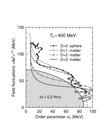
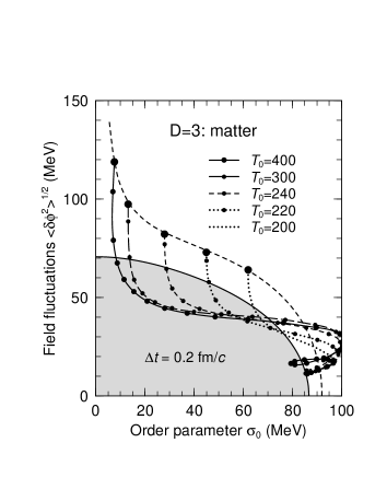
Figure 4: Dynamical trajectories in the plane $\sigma_{0}$–$\langle{\delta\varphi}^{2}\rangle^{1/2}$, where $\sigma_{0}\equiv(\phi_{a}\phi_{a})^{1/2}$, for various expansion scenarios (left) and various initial temperatures (right). The dashed line connects the equilibrium states from $T=0$ to above $500$ MeV and the shaded area corresponds to the instability region where the effective mass (51) is negative. Successive points on a given trajectory are separated by $\Delta t=0.2$ fm/c. From Ref. [68].

The result of the time evolution is most nicely illustrated by plotting the time evolution of the order parameter $\phi^{2}(t)=\phi_{a}(t)\phi_{a}(t)$, where $\phi_{a}(t)\equiv\langle\varphi_{a}({\bf x},t)\rangle$ is the ensemble averaged value of the field at time $t$, versus that of the square fluctuations $\langle{\delta\varphi}^{2}\rangle(t)=\langle\varphi^{2}({\bf x},t)\rangle-\phi^{2}(t)$, where $\varphi^{2}\equiv\varphi_{a}\varphi_{a}$. The corresponding trajectories are shown in Fig. 4 for various initial temperatures and various types of expansions, with $d\equiv D=1,2,3$. Due to the cooling term in the equations of motion, the initial thermal fluctuations are suppressed – the higher the value of $d$, the more efficient the cooling in (52) – and might enter the instability region, where the effective mass squared (51) is negative, represented by the shaded area in Fig. 4. When this happens, long-wavelength modes get amplified. In particular, the order parameter – which is nothing but the zero-mode – grows rapidly and the system is pushed away from the instability region. As expected, we see that the phenomenon is more pronounced for higher values of $d$, corresponding to more rapid expansions. Also, it appears clearly that the time spent in the instability region, which eventually determines the amplitude of the amplification for low-momentum pion modes, strongly depends on the initial temperature: For $T\lesssim 200$ MeV, the initial order parameter is too large and the system never enters the instability region. Similarly, one would expect that for very high initial temperatures $T\gg 500$ MeV, the initial fluctuations are too large for the system to ever become unstable But one observes that there is a large range of temperatures, which roughly correspond to those expected in high-energy nucleus-nucleus collisions, where the expansion produces an efficient quenching of initial fluctuations.

However, a more detailed analysis of the results shown in Fig. 4 reveals that, even for the most favorable case $d=3$, the time spent in the instability region is rather short and barely exceeds $1-1.5$ fm/c. This indicates that the typical trajectories do not get dramatically amplified, in contrast to what happens when the initial fluctuations are artificially quenched deep in the instability region as discussed before. In fact, the ensemble average amplification factor for the most amplified mode $k=0$ was estimated in Ref. [68] to be roughly of order $10$ in the most favorable case. This is very different from the large amplifications, typically $\sim 100$, obtained in the quench scenario. Thus, we can already conclude that, in a more realistic scenario with cooling, large amplifications seem to be a rather rare phenomenon. This conclusion has been corroborated by other studies (see e.g. [73]). A crucial question is, therefore, to know how likely these events are. We shall return to this later in this section (see subsection 2.2.4). We first discuss the issue of describing the quantum corrections to the dynamics in the next subsection.

2.2.3 Quantum corrections to the dynamics

A considerable amount of work has been devoted to include quantum fluctuations in the dynamical description of DCC formation. Initial-value problems in quantum field theory are, however, known to be of notorious difficulty. Existing studies in the context of DCC physics have been mainly limited to the use of mean-field approximations, such as the so-called Hartree approximation, or the large-$N$ approximation. We describe these developments here, for the case of a spherically expanding geometry. We comment on recent progress in non-equilibrium quantum field theory beyond mean-field approximations at the end of this subsection.

Mean-field approximation

In the present context, mean-field approximations consist in replacing the fully non-linear problem by an effective dynamics in a self-adjusting quadratic potential: The system of interacting quantum fields is replaced by an ensemble of independent, self-consistently dressed quasi-particles. There are various ways one can formulate such approximations, such as Gaussian ansätze for the density matrix in the Schrödinger picture [74], Gaussian-like factorization of correlation functions in the Heisenberg equations of motion [74, 68], non-perturbative resummation of so-called daisy and super-daisy diagrams [75], $1/N$-expansion at leading order, where $N=4$ is the number of component of the chiral field [76, 77], etc. Here, we employ the latter approach: the so-called large-$N$ approximation. We shall not enter, however, in the details of the $1/N$-expansion and instead, we give a simple derivation of the equations relevant for our purposes.

The exact Heisenberg equations for the chiral quantum field $\varphi_{a}$ read (see (11)):

$$\left[\square+\lambda(\varphi^{2}(x)-v^{2})\right]\varphi_{a}(x)=H_{a}\,.$$ (53)

As we did previously for the classical field equations (see Eqs. (50)-(51)), we replace the non-linear term in parenthesis by its average $\varphi^{2}\to\langle\varphi^{2}\rangle$, where, here, the brackets denote an average over the initial density matrix $\rho$, which encodes both statistical and quantum fluctuations in the initial state: $\langle\cdots\rangle\equiv{\rm Tr}\{\rho\,\cdots\}/{\rm Tr}\{\rho\}$. Writing the field $\varphi_{a}$ as a sum of its average value $\phi_{a}\equiv\langle\varphi_{a}\rangle$ and a fluctuation field ${\delta\varphi}_{a}$, one gets:

$$\left[\square+\lambda(\phi^{2}(x)+\langle{\delta\varphi}^{2}(x)\rangle-v^{2})\right](\phi_{a}(x)+{\delta\varphi}_{a}(x))=H_{a}\,.$$ (54)

Taking the average of this equation with respect to the initial density matrix $\rho$, one obtain the following non-linear equation for the condensate $\phi_{a}$:

$$\left[\square+M^{2}(x)\right]\phi_{a}(x)=H_{a}\,,$$ (55)

where

$$M^{2}(x)=\lambda\left[\phi^{2}(x)+\langle{\delta\varphi}^{2}(x)\rangle-v^{2}\right]\,.$$ (56)

We see that $\phi_{a}(x)$ evolves in what is essentially the classical potential $V(\phi^{2})=\lambda(\phi^{2}-v^{2})^{2}/4-H\sigma$, modified by quantum and statistical fluctuations through a term $\delta V\propto\langle{\delta\varphi}^{2}\rangle\,\phi^{2}$. Finally, subtracting Eqs. (54) and (55), one obtains the following Klein-Gordon–like equation for the fluctuation field:

$$\left[\square+M^{2}(x)\right]{\delta\varphi}_{a}(x)=0\,.$$ (57)

The excitations of the fluctuation field ${\delta\varphi}_{a}$ describe self-consistently dressed quasi-particles evolving in a $x$-dependent quadratic potential, whose curvature depends on the local value of the condensate and on the mean effect of the fluctuations themselves.

Of course, $\langle{\delta\varphi}^{2}(x)\rangle$ diverges and the above equations require regularization, e.g. through an ultra-violet cut-off $\Lambda$, and renormalization. The quadratic divergence in Eq. (56) can be argued to be $x$-independent by general power-counting arguments and is easily eliminated through the following vacuum subtraction [78]:

$$M^{2}(x)-m_{\pi}^{2}=\lambda\left[\phi^{2}(x)-f_{\pi}^{2}+\langle{\delta\varphi}^{2}\rangle(x)-\langle 0|{\delta\varphi}^{2}|0\rangle\right]$$ (58)

The remaining logarithmic divergence can be eliminated by introducing the renormalized coupling constant [76, 78]:

$$\frac{1}{\lambda_{R}}=\frac{1}{\lambda}+\frac{N}{8\pi^{2}}\int_{0}^{\Lambda}\,\frac{k^{2}dk}{(k^{2}+m_{\pi}^{2})^{3\over 2}}$$ (59)

It is important to notice that the cancellation of the logarithmic divergence at any time requires a suitable choice of initial conditions (see Eqs. (80)-(81) below): Not all initial conditions are physically acceptable. Finally, it should be kept in mind that the present model is at best an effective theory for low-momentum scales. The ultra-violet cut-off has therefore a physical meaning and should be kept finite. The aim of the renormalization procedure is to reduce the cut-off dependence of physical results.

Expanding geometry

We describe the mean-field equations in more details in the case of a spherically expanding system, for which we essentially follow the treatment of Ref. [70]. This requires one to quantify the theory on equal–proper-time hyper-surfaces $\tau={\rm const}$, see Eq. (67) below, where the proper-time $\tau=\sqrt{t^{2}-r^{2}}$, with $r$ the radial distance to the origin, is the time measured by a co-moving observer sitting on an expanding shell. Exploiting the spherical symmetry of the problem, the relevant coordinates are:

$$\tau=\sqrt{t^{2}-r^{2}}\,\,,\,\,\eta=\frac{1}{2}\ln\left(\frac{t+r}{t-r}\right)\,\,,\,\,\hat{\theta}\,\,,\,\,\hat{\varphi}\,\,,$$ (60)

where $\eta$ is the spatial radial rapidity, and $\hat{\theta}$ and $\hat{\varphi}$ the usual azimuthal and polar angles on the sphere. With this choice of coordinates, the relativistic metric is of the Friedrich-Robertson-Walker type and reads, explicitly:

$${\rm d}s^{2}=g_{\mu\nu}\,{\rm d}x^{\mu}{\rm d}x^{\nu}={\rm d}\tau^{2}-\tau^{2}\left(h_{ij}\,{\rm d}x^{i}{\rm d}x^{j}\right)\,,$$ (61)

where $h_{ij}$ is the metric on the $3$–hyperboloïd, or pseudo-sphere, $\tau=1$: $h_{ij}={\rm diag}(1,\sinh^{2}\eta,\sinh^{2}\eta\sin^{2}\hat{\theta})$. The four-dimensional Laplacian reads:

$$\square\equiv\Delta^{(4)}=\partial_{\tau}^{2}+\frac{3}{\tau}\partial_{\tau}-\frac{1}{\tau^{2}}\Delta^{(3)}\,,$$ (62)

where $\Delta^{(3)}$ is the corresponding three-dimensional Laplacian on the unit pseudo-sphere:

$$\Delta^{(3)}=\frac{1}{\sqrt{h}}\,\partial_{i}\,\sqrt{h}\,h^{ij}\,\partial_{j}\,,$$ (63)

with $\sqrt{h}=\sinh^{2}\eta\sin\hat{\theta}$ the determinant and $h^{ij}$ the inverse of the three-dimensional metric $h_{ij}$.

Spherical symmetry and radial-boost invariance ensures that both the condensate $\phi_{a}$ and the effective mass $M^{2}$ only depend on the proper-time $\tau$ and Eq. (55) reads:

$$\ddot{\phi}_{a}(\tau)+\frac{3}{\tau}\,\dot{\phi}_{a}(\tau)+M^{2}(\tau)\,\phi_{a}(\tau)=H_{a}\,,$$ (64)

The canonical quantization of the fluctuation field is more conveniently formulated in terms of the dimensionless rescaled fields (the various components of the fluctuation field ${\delta\varphi}_{a}$ being all equivalent in the present approximation, Eq. (57), we drop the chiral indices for simplicity):

$$\varphi(\tau,{\bf x}) = \tau{\delta\varphi}(\tau,{\bf x})$$ (65)

$$\pi(\tau,{\bf x}) = \tau\dot{\varphi}(\tau,{\bf x})=\varphi^{\prime}(\tau,{\bf x})$$ (66)

where the dot represents the derivation with respect to $\tau$ and the prime represents the derivation with respect to the conformal-time variable $u=\ln\tau/\tau_{0}$. These operators satisfy the equal-time commutation relations:

$$\left[\varphi(\tau,{\bf x}),\pi(\tau,{\bf x}^{\prime})\right]=i\,\delta_{{\bf x},{\bf x}^{\prime}}\,,$$ (67)

where we introduced the short-hand notations ${\bf x}\equiv(\eta,\hat{\theta},\hat{\varphi})$ and $\delta_{{\bf x},{\bf x}\,^{\prime}}\equiv\delta(\eta-\eta^{\prime})\delta(\hat{\theta}-\hat{\theta}^{\prime})\delta(\hat{\varphi}-\hat{\varphi}^{\prime})/\sqrt{h}$. Exploiting the symmetry of the problem, one projects the fluctuation field $\varphi$ on eigenfunctions of the three-dimensional Laplacian (63):

$$\varphi_{\bf s}(\tau) = \int d^{3}x\sqrt{h}\,{\mathcal{Y}}_{\bf s}^{*}({\bf x})\,\varphi(\tau,{\bf x})$$ (68)

$$\pi_{\bf s}(\tau) = \int d^{3}x\sqrt{h}\,{\mathcal{Y}}_{\bf s}^{*}({\bf x})\,\pi(\tau,{\bf x})\,,$$ (69)

where the so-called hyperbolic harmonics are defined as [81, 82]:

$$\Delta^{(3)}\,{\mathcal{Y}}_{{\bf s}}({\bf x})=-(s^{2}+1)\,{\mathcal{Y}}_{{\bf s}}({\bf x})\,.$$ (70)

Here we introduced the notation ${\bf s}\equiv(s,l,m)$, where $s$ is a positive real variable and $l$ and $m$ take integer values: $0\leq l<+\infty$ and $-l\leq m\leq l$. The hyperbolic harmonics form an orthonormal basis, spanning the space of functions on the unit pseudo-sphere. One has, in particular:

$$\int d^{3}x\,\sqrt{h}\,\,{\mathcal{Y}}_{{\bf s}^{\prime}}^{*}({\bf x})\,{\mathcal{Y}}_{{\bf s}}({\bf x})=\delta_{{\bf s},{\bf s}^{\prime}}\,,$$ (71)

where $\delta_{{\bf s},{\bf s}^{\prime}}\equiv\delta(s-s^{\prime})\,\delta_{ll^{\prime}}\,\delta_{mm^{\prime}}$.

In the mean-field approximation, the equations of motion (57) for the fluctuation field are essentially linear and the most general solution can, therefore, be written as:

$$\varphi_{\bf s}(\tau) = \psi_{s}(\tau)\,a_{\bf s}+\psi^{*}_{s}(\tau)\,(-1)^{m}\,a^{\dagger}_{-{\bf s}}$$ (72)

$$\pi_{\bf s}(\tau) = \psi_{s}^{\prime}(\tau)\,a_{\bf s}+\psi^{*^{\prime}}_{s}(\tau)\,(-1)^{m}\,a^{\dagger}_{-{\bf s}}\,,$$ (73)

where, as before, the prime denotes differentiation with respect to $u=\ln\tau/\tau_{0}$. The annihilation and creation operators $a_{\bf s}$ and $a^{\dagger}_{{\bf s}}$ for quasi-particle excitations satisfy the following commutation relations:

$$[a_{{\bf s}},a^{\dagger}_{{\bf s}^{\prime}}]=\delta_{{\bf s},{\bf s}^{\prime}}\,,$$ (74)

all other commutators being zero. The corresponding mode functions $\psi_{s}(\tau)$ satisfy the following differential equation:

$$\ddot{\psi}_{s}(\tau)+\frac{1}{\tau}\dot{\psi}_{s}(\tau)+\omega_{s}^{2}(\tau)\psi_{s}(\tau)=0\,,$$ (75)

which describes a set of damped oscillators with time-dependent frequencies:

$$\omega_{s}(\tau)=\sqrt{\frac{s^{2}}{\tau^{2}}+M^{2}(\tau)}\,.$$ (76)

The physical momentum of the corresponding quasi-particle, $k=s/\tau$, is red-shifted as time increases, as a simple consequence of expansion. In terms of the variable $u=\ln\tau/\tau_{0}$, one has:

$$\psi_{s}^{\prime\prime}(\tau)+\tilde{\omega}_{s}^{2}(\tau)\,\psi_{s}(\tau)=0\,,$$ (77)

where $\tilde{\omega}_{s}(\tau)=\tau\omega_{s}(\tau)$ is a dimensionless frequency. The problem therefore reduces to the familiar one of a set of parametrically excited oscillators. The non-linear character of the mean-field dynamics enters through the calculation of the self consistent mass, Eq. (56). For instance, assuming that in the initial state:

$$\langle a_{\bf s}^{\dagger}a_{{\bf s}^{\prime}}\rangle=n_{s}^{(a)}\,\delta_{{\bf s},{\bf s}^{\prime}}\quad,\quad\langle a_{\bf s}a_{{\bf s}^{\prime}}\rangle=0\,,$$ (78)

one has, using the property $\sum_{lm}\,|{\mathcal{Y}}_{{\bf s}}({\bf x})|^{2}=s^{2}/2\pi^{2}$ [81]:

$$\frac{M^{2}(\tau)}{\lambda}=\phi^{2}(\tau)-v^{2}+\frac{N}{\tau^{2}}\int_{0}^{\Lambda\tau}\frac{s^{2}ds}{2\pi^{2}}\,|\psi_{s}(\tau)|^{2}\,(2n_{s}+1)\,,$$ (79)

where $N=4$ is the number of components of the chiral field. The integral on the RHS is limited to physical momenta $k=s/\tau\leq\Lambda$. Finally, the quantization is completed by choosing appropriate initial conditions for the mode functions. The cancellation of divergences required by the renormalization of the mass gap is ensured if one adopts the following adiabatic condition at $\tau=\tau_{0}$:

$$\psi_{s}(\tau_{0}) = \frac{1}{\sqrt{2\tilde{\omega}_{s}(\tau_{0})}}$$ (80)

$$\psi_{s}^{\prime}(\tau_{0}) = -i\sqrt{\frac{\tilde{\omega}_{s}(\tau_{0})}{2}}\left[1-i\frac{\tilde{\omega}_{s}^{\prime}(\tau_{0})}{2\tilde{\omega}_{s}^{2}(\tau_{0})}\right]\,.$$ (81)

Physical particles, interpolating field and amplification factor

Assume that Heisenberg and Schrödinger representations coincide at $\tau=\tau_{0}$. With the choice (80)-(81) of initial mode functions, one can regard $a_{\bf s}^{\dagger}$ as the Schrödinger representation operator creating a particle with frequency $\omega_{s}(\tau_{0})$. These are the physical excitations appropriate for the description of the initial state. Similarly, one can introduce the particles with frequencies $\omega_{s}(\tau_{f})$ appropriate to the final state at $\tau=\tau_{f}$. Let $b^{\dagger}_{\bf s}$ denote the corresponding creation operator in the Schrödinger representation. The Heisenberg representation field operators, given by (72)-(73), can then also be written as:

$$\varphi_{\bf s}(\tau) = q_{s}\,b_{\bf s}(\tau)+q^{*}_{s}\,(-1)^{m}\,b^{\dagger}_{-{\bf s}}(\tau)$$ (82)

$$\pi_{\bf s}(\tau) = p_{s}\,b_{\bf s}(\tau)+p^{*}_{s}\,(-1)^{m}\,b^{\dagger}_{-{\bf s}}(\tau)\,,$$ (83)

with

$$q_{s} = \frac{1}{\sqrt{2\tilde{\omega}_{s}(\tau_{f})}}$$ (84)

$$p_{s} = -i\sqrt{\frac{\tilde{\omega}_{s}(\tau_{f})}{2}}\left[1-i\frac{\tilde{\omega}_{s}^{\prime}(\tau_{f})}{2\tilde{\omega}_{s}^{2}(\tau_{f})}\right]\,,$$ (85)

and

$$b_{\bf s}(\tau)=U(\tau,\tau_{0})\,b_{\bf s}\,U^{\dagger}(\tau,\tau_{0})\,,$$ (86)

where $U(\tau,\tau_{0})$ denotes the unitary time-evolution operator, which connects the Heisenberg and Schrödinger representations. Using (72)-(73) and (82)-(83), one easily obtains the Bogolyubov transformation connecting the operators $a_{\bf s}$, $a^{\dagger}_{\bf s}$ and $b_{\bf s}(\tau)$, $b^{\dagger}_{\bf s}(\tau)$:

$$b_{\bf s}(\tau) = \alpha_{s}(\tau)\,a_{\bf s}+\beta_{s}(\tau)\,(-1)^{m}\,a^{\dagger}_{-{\bf s}}$$ (87)

$$(-1)^{m}\,b^{\dagger}_{-{\bf s}}(\tau) = \beta^{*}_{s}(\tau)\,a_{\bf s}+\alpha^{*}_{s}(\tau)\,(-1)^{m}\,a^{\dagger}_{-{\bf s}}\,,$$ (88)

where

$$i\alpha^{*}_{s}(\tau) = q_{s}\,\psi^{*^{\prime}}_{s}(\tau)-p_{s}\,\psi^{*}_{s}(\tau)$$ (89)

$$i\beta^{*}_{s}(\tau) = q_{s}\,\psi_{s}^{\prime}(\tau)-p_{s}\,\psi_{s}(\tau)\,.$$ (90)

Figure 5: Proper-time evolution of the effective mass squared $M^{2}(\tau)$ for the initial condition of Ref. [70], namely: $\phi_{a}(\tau_{0})=(0.3,{\vec{0}})$ [fm^-1] and $\dot{\phi}_{a}(\tau_{0})=(-1,{\vec{0}})$ [fm^-2], at $\tau_{0}=1$ fm. The initial temperature is $T=200$ MeV. The employed parameters are: $\Lambda=800$ MeV, $m_{\pi}=139.5$ MeV, $f_{\pi}=92.5$ MeV and $\lambda_{R}=7.3$. The dashed line shows the value of the pion mass squared $m_{\pi}^{2}=0.5$ fm^-2.

Figure 6: The amplification factor ${\mathcal{A}}_{s}(\tau_{f})$ corresponding to the event of Fig. 5, for various values of the final time $\tau_{f}$.

Assuming that the initial state is characterized by the correlations (78), one finally obtains the number of $b$-particles at the final time $\tau_{f}$ for a given number of $a$-particles at the initial time $\tau_{0}$ as:

$$n^{(b)}_{s}(\tau_{f})+\frac{1}{2}={\mathcal{A}}_{s}(\tau_{f})\left(n^{(a)}_{s}+\frac{1}{2}\right)\,,$$ (91)

where $n^{(b)}_{s}(\tau)\equiv\langle b_{\bf s}^{\dagger}(\tau)b_{\bf s}(\tau)\rangle$. The amplification factor is given by:

$${\mathcal{A}}_{s}(\tau_{f})=1+2\,|\beta_{s}(\tau_{f})|^{2}\,.$$ (92)

Figure 5 shows the time evolution of the effective mass squared $M^{2}(\tau)$ for a particular set of initial conditions, taken from Ref. [70]. Here, one assumes a local thermal equilibrium at temperature $T$ in the initial state and sets, accordingly:

$$n^{(a)}_{s}=\frac{1}{{\rm e}^{\omega_{s}(\tau_{0})/T}-1}\,.$$ (93)

One sees that, for the considered initial conditions (see the caption of Fig. 5), the system is driven into the unstable region and the effective mass squared becomes negative for some period of time. This leads to a dramatic amplification of low-momentum modes, as shown in Fig. 6. Notice that due to the freeze-out of interactions at large enough $\tau_{f}$, one has $M^{2}(\tau_{f})\simeq m_{\pi}^{2}$ and the particles in the final state indeed correspond to physical pions. These results are the quantum analog of those obtained previously using classical statistical field theory techniques and demonstrates that significant amplifications can be obtained for some appropriate choice of initial conditions $(\phi_{a}(\tau_{0}),\dot{\phi}_{a}(\tau_{0}))$.

Non-equilibrium dynamics beyond the mean-field approximation

Mean-field approximations, such as the large-$N$ approximation employed above, neglect scatterings between quasi-particles. The latter tend to redistribute the energy stored in the amplified modes among other modes and to thermalize the system, hence washing out any signal in the final state. It is a crucial issue for the quench scenario to be successful, that freeze-out occurs before the early-time amplification get washed out.

The description of the far-from-equilibrium dynamics of quantum fields beyond mean-field–like approximations has long been a major difficulty in practice: Similar to perturbation theory, standard approximation schemes, such as e.g. a coupling or a $1/N$-expansion of the one-particle-irreducible (1PI) effective action, are plagued by the problem that a secular (unbounded) time evolution prevents the study of the late-time behavior. Important progress in this field has been made in recent years with the use of efficient functional integration techniques, so-called $n$-particle-irreducible (nPI) effective actions [83, 84, 85], for which practicable non-perturbative expansion schemes are available. In particular, it has been demonstrated that approximations based on a systematic coupling or $1/N$-expansion of the 2PI effective action allow for practical, first principle calculations of the far-from-equilibrium dynamics as well as late-time quantum thermalization [86].

Clearly, it would be of definite interest to apply these methods to the problem of DCC formation. For instance, the large-$N$ calculation described in the previous subsection can be systematically improved using the 2PI $1/N$-expansion [88, 89]. In particular, this provides a valid description of the dynamics at non-perturbatively high occupation numbers [90], as is the case in the context of the out-of-equilibrium chiral phase transition.

2.2.4 The likelihood of DCC formation

The quench scenario provides a plausible mechanism for DCC formation in high-energy heavy-ion collisions. A proper description of the cooling due to expansion reveals, however, that significantly large amplifications are not very likely. It is therefore crucial for phenomenology to estimate the probability that this happens. It is true that the present models are not realistic enough to be trusted at the quantitative level. Nevertheless, even within the existing framework it is legitimate to seek for a crude estimate of the probability in question. This problem has been addressed in Ref. [26] (see also [73]), which we review in the present subsection.

Physical picture and sampling strategy

Consider the evolution of a spherical droplet of DCC in its rest frame. One starts with a small ball of radius $R_{0}$, filled with hot matter in local thermal equilibrium at a temperature $T$ and assumes that the ball undergoes a radial expansion at the speed of light. Due to the time dilation the temperature stays approximately constant within a layer near the boundary of the ball. The equations of motion of the sigma model are supposed to describe what happens in the interior of the ball, the cooling observed as one moves away from the surface towards the center. As a first approximation, it is simpler to assume that the expanding bubble is connected forever to a heat bath kept at constant temperature $T$, so that the process never stops. Of course, the hot shell becomes thinner with increasing time and eventually disappears. We shall discuss the effect of switching the heat bath off at the end of this subsection. The relevant boundary conditions for the pion field inside the bubble are specified on the hyper-surface $\tau=\tau_{0}=R_{0}$, where the proper-time $\tau=\sqrt{t^{2}-r^{2}}$, with $r$ the radial coordinate. A given field configuration completely determines the amplitude of the resulting pionic amplification. The point is that the probability of occurrence of a particular initial field configuration can be completely determined once one has assumed that the initial droplet is in local thermal equilibrium.

The quantum evolution of the system is treated in the large-$N$ approximation discussed previously. In that case, one can convince oneself (see also footnote 27 above) that the only relevant initial conditions are those concerning the average-value of the field $\phi_{a}(\tau_{0})$ and its proper-time derivative $\dot{\phi}_{a}(\tau_{0})$. For the sake of the argument, consider first the case of a classical field. The key observation is to realize that an observer living within the ball cannot distinguish the initial values $\phi_{a}(\tau_{0})$ and $\dot{\phi}_{a}(\tau_{0})$ from the spatial averages $\bar{\phi}_{a}$ and $\bar{\pi}_{a}$ of the field and of its time derivative respectively, calculated over the volume $V_{0}$ of the initial ball. The point is that the latter variables fluctuate in a predictable manner: Assuming that the initial ball, of fixed volume $V_{0}$, is in local thermal equilibrium at temperature $T$ means that the field fluctuates as if the ball were part of a larger system, with volume $V$ much larger than $V_{0}$, in equilibrium at the same temperature $T$. In this large system the variances of the spatial averages of the field and of its time derivative are very small, of order $1/V$ (since long range correlations are absent). The corresponding variances for spatial averages over the volume of the ball are just the same, enhanced by a factor of order $V/V_{0}$ (assuming that the radius of the ball is at least of the order of the correlation length at temperature $T$).

In the quantum theory, the $c$-numbers $\bar{\phi}_{a}$ and $\bar{\pi}_{a}$ correspond to the possible measured values of the observables:

$$\bar{\Phi}_{a} = \frac{1}{V_{0}}\int_{V_{0}}d^{3}x\,\varphi_{a}({\bf x})$$ (94)

$$\bar{\Pi}_{a} = \frac{1}{V_{0}}\int_{V_{0}}d^{3}x\,\dot{\varphi}_{a}({\bf x})\,,$$ (95)

They can be sampled from the probability distribution characterized by the means:

$${\rm E}[\bar{\phi}_{a}] = \langle\bar{\Phi}_{a}\rangle_{{}_{T}}=\frac{H}{M^{2}_{T}}\,\delta_{a,\sigma}\,,$$ (96)

$${\rm E}[\bar{\pi}_{a}] = \langle\bar{\Pi}_{a}\rangle_{{}_{T}}=0\,,$$ (97)

and by the variances (no sum over $a$):

$${\rm Var}\left[\bar{\phi}_{a}\right]=\langle\bar{\Phi}_{a}^{2}\rangle_{{}_{T}}-\langle\bar{\Phi}_{a}\rangle_{{}_{T}}^{2}=\frac{1}{V_{0}^{2}}\,\int_{V_{0}}d^{3}xd^{3}y\,\langle{\delta\varphi}_{a}({\bf x}){\delta\varphi}_{a}({\bf y})\rangle_{{}_{T}}$$ (98)

and

$${\rm Var}\left[\bar{\pi}_{a}\right]=\langle\bar{\Pi}_{a}^{2}\rangle_{{}_{T}}-\langle\bar{\Pi}_{a}\rangle_{{}_{T}}^{2}=\frac{1}{V_{0}^{2}}\,\int_{V_{0}}d^{3}xd^{3}y\,\langle\delta\dot{\varphi}_{a}({\bf x})\delta\dot{\varphi}_{a}({\bf y})\rangle_{{}_{T}}\,,$$ (99)

where thermal averages $\langle\dots\rangle_{{}_{T}}$ correspond to the equilibrium density matrix $\rho\propto\exp(-H/T)$, with $H$ the Hamiltonian. The thermal correlators in Eqs. (98) and (99) can be written as:

$$\langle{\delta\varphi}_{a}({\bf x}){\delta\varphi}_{a}({\bf y})\rangle_{{}_{T}}=\int\frac{d^{3}k}{(2\pi)^{3}}\,G^{a}_{T}(k)\,{\rm e}^{i\,{\bf k}\cdot({\bf x}-{\bf y})}\,,\\$$

and similarly for $\langle\delta\dot{\varphi}_{a}({\bf x})\delta\dot{\varphi}_{a}({\bf y})\rangle_{{}_{T}}$ with $G^{a}_{T}(k)\to K^{a}_{T}(k)$. In the large-$N$ approximation, one has: $G^{a}_{T}(k)=\coth(E_{k}/2T)/2E_{k}$ and $K^{a}_{T}(k)=E_{k}^{2}G^{a}_{T}(k)$, where $E_{k}=\sqrt{k^{2}+M_{T}^{2}}$. Here, the equilibrium mass-gap at temperature $T$, $M_{T}$, is the solution of the gap-equation (56) written in thermal equilibrium:

$$\frac{M^{2}_{T}}{\lambda}=\phi_{T}^{2}-v^{2}+N\int\frac{d^{3}k}{(2\pi)^{3}}\,\frac{\coth(E_{k}/2T)}{2E_{k}}\,,$$ (100)

where $\phi_{T}=H/M^{2}_{T}$ is the thermal condensate (cf. Eq. (96)).

In the large-$N$ approximation the interacting system is effectively replaced by an ensemble of independent excitations with mass $M_{T}$ and the probability distribution we are interested in is, therefore, simply given by a Gaussian. The latter is completely characterized by the parameters given in (96)-(99). The variances (98)-(99) can be estimated analytically when the radius $R_{0}$ of the ball is much larger than the correlation length $\lambda_{T}=1/M_{T}$. In that case, it is sufficient to calculate the variances for the quasi-infinite volume $V$ and to multiply the result by $V/V_{0}$, since the $V/V_{0}$ small cells fluctuate independently. Obviously, only the modes $k\lesssim 1/R_{0}$ contribute to the integrals in Eqs. (98)-(99). Therefore, for large volumes, there is only the zero mode contribution and one immediately gets:

$${\rm Var}\left[\bar{\phi}_{a}\right] \approx \frac{G^{a}_{T}(0)}{V_{0}}=\frac{1}{2V_{0}M_{T}}\,\coth\left(\frac{M_{T}}{2T}\right)\,,$$ (101)

$${\rm Var}\left[\bar{\pi}_{a}\right] \approx \frac{K^{a}_{T}(0)}{V_{0}}=\frac{M_{T}}{2V_{0}}\,\coth\left(\frac{M_{T}}{2T}\right)\,.$$ (102)

The dispersion of $\bar{\phi}_{a}$ calculated exactly [91] is smaller by a factor of $2$ ($1.5$) for $R_{0}=\lambda_{T}$ ($R_{0}=2\lambda_{T}$) and $T=200$ to $400$ MeV. The dispersion of $\bar{\pi}_{a}$ obtained from (99) differs from the estimation (102) by 20% (8%), respectively. For $R_{0}<\lambda_{T}$ the discrepancy between the analytical formulas and the exact results increases rapidly [91]. Finally, as expected, the fluctuations within the ball depend rather weakly on the environment provided $R_{0}\gtrsim\lambda_{T}$.

The formalism of Ref. [70], reviewed in subsection 2.2.3 above, together with the sampling method proposed in Ref. [26], and described above, enable one to estimate the likelihood of a coherent amplification of the pion field. More precisely, one can calculate the probability that the amplification factor $A_{s}$ given by Eq. (92) takes a given value. In such a calculation the size $R_{0}$ of the initial ball appears as a free parameter. Remember, however, that one has to set $\tau_{0}=R_{0}$ and that the friction force responsible for the quench is proportional to $1/\tau$. Thus the likelihood of DCC formation decreases with increasing $R_{0}$. This parameter should be assigned the smallest possible value in order to get an upper bound for the probability we are looking for.

At this point, it is important to realize that the model described here only makes sense for $R_{0}\gtrsim\lambda_{T}$. Indeed, the concept of local thermal equilibrium is meaningful for a cell whose degrees of freedom fluctuate more or less independently from what happens in the neighbouring cells. Also, the validity of the mean-field approximation requires the size of the cell to be larger than the Compton wavelength of a typical excitation. With these arguments in mind, one focuses on the values of $R_{0}$ in the range of one or two correlation length.

Results

Figure 7: Probability distribution of the amplification factor $A$ of the softest mode for various choices of the initial temperature $T$ and size of the ball $R_{0}$ (in units of the correlation length). All histogram are made from at least $10^{4}$ events. From Ref. [26].

Figure 8: The strengths of the initial classical iso-vector and iso-axial-vector currents, ${\vec{V}}_{\mu}\cdot{\vec{V}}^{\mu}$ and ${\vec{A}}_{\mu}\cdot{\vec{A}}^{\mu}$ respectively (in fm^-6), versus the amplification factor $A$. The parameters are $R_{0}=\lambda_{T}$ and $T=200$ MeV. From Ref. [26].

The main result of Ref. [26] is reproduced in Fig. 7, which shows the histograms of the probability $P(A)$ that the amplification factor of the $s=0^{+}$ mode takes the value $A_{0}=A$. The relevant parameters are the same as in Ref. [70], see Figs. 5 and 6. The amplification is calculated at $\tau_{f}=10$ fm/c, where the system is in the stationary regime. Clearly, large amplifications occurs in a small fraction of events only. It is interesting to notice that one condition for a large amplification appears to be the smallness of the absolute strength of the initial classical iso-vector current ${\vec{V}}_{\mu}={\vec{\pi}}_{0}\times\partial_{\mu}{\vec{\pi}}_{0}$ as compared to that of the corresponding axial current ${\vec{A}}_{\mu}={\vec{\pi}}_{0}\partial_{\mu}\sigma_{0}-\sigma_{0}\partial_{\mu}{\vec{\pi}}_{0}$, where $({\vec{\pi}}_{0},\sigma_{0})\equiv\phi_{a}(\tau_{0})$ and $(\dot{\vec{\pi}}_{0},\dot{\sigma}_{0})\equiv\dot{\phi}_{a}(\tau_{0})$. This is illustrated by the histograms of Fig. 8, which shows the the respective currents versus the amplification factor $A$. Recall that a similar condition was required in order that the classical solution of Blaizot and Krzywicki, described in Sec. 2.1, actually corresponds to a DCC, that is to a linearly polarized in isospin space.

In order to judge what amplification should be considered as large for phenomenological purposes, one can estimate the multiplicity of produced pions. The invariant one-pion inclusive spectrum can be obtained as [92]:

$$E\frac{dn}{d^{3}p}=\int d^{4}x\sqrt{-g}\,\delta(\tau-\tau_{f})\,f(x,p)\,p^{\mu}u_{\mu}$$ (103)

where $g$ is the determinant of the metric tensor, see (61), $f(x,p)$ is the invariant phase-space density of produced particles and $u^{\mu}=dx^{\mu}/d\tau=x^{\mu}/\tau$ is the $4$-velocity of the co-moving volume centered at $x^{\mu}$. It is a unit $4$-vector orthogonal to the hyper-surface $\tau=\tau_{f}$, where the particles are counted. In the present case, one has [26]: $f(x,p)=N(2\pi)^{-3}n^{(b)}_{s}(\tau_{f})$, where $n^{(b)}_{s}(\tau_{f})$ is given by Eq. (91) above. The momentum $s/\tau_{f}$ in the expanding frame is related to the $4$-momentum $p^{\mu}$ in the rest frame by the obvious relation [70] (see Eq. (76)):

$$p^{\mu}u_{\mu}=\omega_{s}(\tau_{f})=\sqrt{\frac{s^{2}}{\tau_{f}^{2}}+M^{2}_{f}}\,,$$ (104)

where $M^{2}_{f}=M^{2}(\tau_{f})\approx m_{\pi}^{2}$ is the mass gap at time $\tau_{f}$. In the present case, the integrand in (103) depends on a single external $4$-vector, i.e. $p^{\mu}$, and therefore the integral, being a Lorentz scalar, only depends on $p^{2}=M_{f}^{2}$: The invariant spectrum is flat. Using hyperbolic coordinates, see Eq. (60), one finally obtains [91]:

$$E\frac{dn}{d^{3}p}\,({\bf p})=E\frac{dn}{d^{3}p}\,({\bf p}=0)=\frac{N}{M^{2}_{f}}\int_{0}^{\Lambda\tau_{f}}\frac{s^{2}ds}{2\pi^{2}}\,n^{(b)}_{s}(\tau_{f})\,.$$ (105)

Notice that the RHS of Eq. (105) does not depend on the choice of $\tau_{f}$, provided the latter is large enough (see also Fig. 6).

The flatness of the spectrum is, of course, an artifact of the unrealistic assumption that the boost invariant expansion continues forever. In a real collision process the expansion would last a finite time and the resulting spectrum would be cut, the value of the cut-off reflecting the behavior of the environment. Obviously, the predicted total multiplicity depends strongly on this cut-off and cannot be estimated in a reliable manner within the present model. However, the RHS of (105) is presumably a reasonable estimate of the invariant momentum-space density of soft pion radiation (see, however, [35]). The latter can be compared to the corresponding density of incoherently produced pions. A simple example is instructive: The one-particle spectrum in the central rapidity region of a heavy-ion collision can be parametrized as follows:

$$\left.E\frac{dn}{d^{3}p}\right|_{inc}=\left.\frac{dn}{dyd^{2}p_{t}}\right|_{inc}=\frac{h}{\pi\langle p_{t}^{2}\rangle}\exp\left(-\frac{p_{t}^{2}}{\langle p_{t}^{2}\rangle}\right)\,,$$ (106)

where $h$ denotes the height of the rapidity plateau. In a central Pb-Pb collision at the CERN SPS one observes [93] about 200 $\pi^{-}$ per unit rapidity, i.e. for all pions $h\approx 600$. Thus the invariant momentum space density at very small transverse momentum is roughly $1900$ GeV^-2, using $\langle p_{t}^{2}\rangle=0.1$ GeV². The corresponding density fluctuation is expected to be $\sim\sqrt{h}/\pi\langle p_{t}^{2}\rangle\approx 75$ GeV^-2. For the DCC signal to be detectable, the RHS of (105) should be significantly larger than the expected fluctuation. One finds [26] that the signal is more than three times the fluctuation for events where the amplification factor for the zero mode is $A\gtrsim 45$. Setting $R_{0}=\lambda_{T}$, the corresponding probability is roughly $4\times 10^{-3}$ both for $T=200$ MeV and $T=400$ MeV. Of course, this is a conditional probability, as it has been assumed that the initial plasma droplet was formed in the collision. Moreover, one should keep in mind that the present estimate has been obtained in the most favorable scenario and should, therefore, be considered as an upper-bound.

Thus, the probability of a potentially observable DCC signal appears small. The present crude estimate indicates that in a central Pb-Pb collision at CERN SPS this probability is at best:

$${\rm Probability}(\mbox{``observable'' DCC})\lesssim 10^{-3}\,.$$ (107)

This should be taken into account by experimenters designing DCC hunt strategies as well as theorists studying possible DCC signatures. It is worth emphasizing that the above prediction agrees with the present experimental upper limits for DCC formation obtained at CERN by both the WA98 and the NA49 collaborations [18, 19, 21].

2.2.5 The unpolarized DCC

The quench scenario has been widely accepted as a microscopic description of DCC formation in heavy-ion collisions and, as such, has been extensively used to study DCC phenomenology [94, 95, 71], see Sec. 2.4. However, if the rapid suppression of initial fluctuations indeed provides a robust mechanism for the formation of a strong coherent pion field, it is not clear whether it can explain the hypothetical polarization in iso-space originally proposed (see e.g. Eq. (7)). In fact, the expected large event-by-event fluctuations of the neutral ratio, see Eq. (10), have never been observed in actual simulations of the out-of-equilibrium phase transition [96, 94, 95]. Of course, deviations from the ideal law (10) are to be expected in a realistic situation, but the complete absence of large fluctuations in the quench scenario suggests that the original picture of linearly polarized waves coherently aligned in isospin space might actually not be realized in the context of the far-from-equilibrium chiral phase transition.

Figure 9: Neutral fraction distribution in a single mode, here ${\bf k}=0$, at initial time (dashed line) and at final time, here $t_{f}=10$ fm (histogram). From Ref. [97].

It is a question of great phenomenological relevance to inquire to what extent is the original picture realized in a realistic microscopic model. The point is that the usual assumption of a (locally) thermalized initial state implies that the field modes are completely uncorrelated at initial time. In order to actually generate a DCC configuration, the microscopic mechanism at work needs not only to be efficient in amplifying the modes amplitudes, but it should also build correlations between amplified modes. This question has been investigated in Ref. [97], where a detailed statistical analysis of the pion field configurations produced after a quench has been performed, with particular emphasis on their isospin structure. For this purpose, it is sufficient to consider the original model of Rajagopal and Wilczek [10], see subsection 2.2.1, which includes all the relevant physical features. In particular, the classical field approximation allows one to take into account the full non-linear character of the problem, which is crucial to study correlations. Moreover, in the quench approximation, the system is artificially prepared in an unstable situation, all configurations undergo a dramatic amplification, as in Fig. 1. This automatically selects the events which are relevant for the present analysis.

Figure 10: Normalized correlation between the fluctuations of the neutral fraction in the zero mode and in mode k as a function of momentum. From Ref. [97].

Figure 11: Event-by-event distribution of the neutral fraction in a bin in momentum space containing 10 amplified modes. The expected DCC signal is already considerably reduced, due to the absence of correlation between modes. From Ref. [97].

To analyze the isospin orientations of distinct field modes, a sensitive observable is the neutral fraction of pions in each mode ${\bf k}$, defined as:

$$f({\bf k})=\frac{\bar{n}_{3}({\bf k})}{\bar{n}_{1}({\bf k})+\bar{n}_{2}({\bf k})+\bar{n}_{3}({\bf k})}\,,$$ (108)

where $\bar{n}_{a}({\bf k})\equiv\bar{n}_{a}({\bf k},t_{f})$ represent the averaged occupation numbers corresponding to the classical field configuration at the final time $t_{f}$, see Eq. (49). The event-by-event distribution of the neutral fraction (108) for the most amplified mode, ${\bf k}=0$, is shown in Fig. 9 for $t_{f}=10$ fm/c, corresponding roughly to the end of the spinodal instability period, cf. Fig. 2. The corresponding distribution at time $t_{f}=56$ fm/c, characteristic of the parametric amplification mechanism, looks exactly the same [97]. In both cases, all the amplified modes exhibit similar distributions. In fact, the neutral fraction distributions for amplified modes are found to be essentially the same as the corresponding ones in the initial state. The latter can be computed exactly [97, 91] and is represented by the dashed line in Fig. 9. For a given mode ${\bf k}$, it reads:

$$P_{k}(f)=\frac{1}{2}\Big{[}F_{\Omega_{k}}(f)+F_{-\Omega_{k}}(f)\Big{]}\,,$$ (109)

where

$$F_{\Omega}(f)=[\Omega-(1-f)]\left(\frac{\Omega+1}{\Omega-(1-2f)}\right)^{3/2}\,,$$ (110)

and

$$\Omega_{k}=\frac{\sigma_{2}^{2}+\omega_{k}^{2}\sigma_{1}^{2}}{\sigma_{2}^{2}-\omega_{k}^{2}\sigma_{1}^{2}}\,.$$ (111)

with $\sigma_{1}^{2}$ and $\sigma_{2}^{2}$ the variances of the field and its time derivative respectively (see subsection 2.2.1). Although not exactly $1/\sqrt{f}$, the distribution is very broad, exhibiting large fluctuations around the mean value $\bar{f}=1/3$, which is the relevant point for phenomenology. As emphasized previously, these large fluctuations are a direct manifestation of the classical nature of the field modes. The deviations from the ideal law (10) come from the fact that the latter are not strictly linearly polarized waves [97].

However, one finds that distinct modes have completely independent polarizations in isospin space, as can be seen on Fig. 10, which shows the statistical correlation between the neutral fractions in different amplified modes: Their directions of oscillation in isospin space are completely random. In other words, different modes act as independent DCCs. This has the important phenomenological consequence that the large event-by-event fluctuations of the neutral fraction are rapidly washed out when the contributions of several modes are added in a momentum bin, even when one limits one’s attention to soft modes only. This is illustrated in Fig. 11, which shows the neutral fraction distribution in a bin containing $10$ modes. The expected signal is considerably reduced, already for such a small bin. This explains the absence of large fluctuations reported in previous studies [96, 94, 95], where the authors typically considered the contribution of a large number of modes.

Figure 12: Schematic representation of the ideal DCC configuration (left), where all field modes oscillate in the same direction in isospin space (see Eq. (10)), and of the unpolarized DCC formed after a quench (right), where the modes have independent directions of oscillation.

In conclusion, the non-linear dynamics of the linear sigma model does not build the required correlation between modes: The state produced in the simplest form of the quench scenario, where no correlations are present initially, is not identical to the originally proposed DCC. Instead, a more realistic picture is that of a superposition of waves having independent orientations in isospin space: an “unpolarized” DCC configuration, as depicted on Fig. 12. Of course, one cannot exclude the possibility that the required correlations between modes be indeed (partially) formed in actual nuclear or hadronic collisions by means of some other mechanism. Reality most probably lies between the two extreme pictures represented on Fig. 12. The point is that the only presently existing microscopic scenario for DCC formation predicts an unpolarized state. This information should be taken into account in further theoretical as well as experimental investigations.

2.3 Lifetime of the DCC

So far we have been mainly concerned with the description of the intrinsic DCC dynamics, that is the possible mechanism responsible for its formation. We now discuss extrinsic aspects of DCC dynamics, namely those concerning the interactions of the DCC bubble with its hadronic environment. If at all, the DCC is produced in a high-multiplicity environment and must be considered as an open system interacting with the surrounding degrees of freedom [100]. In the context of ultra-relativistic heavy-ion collisions, one typically imagines a thermal bath of pions and nucleons. The interactions with the latter tend to destroy the coherence of the DCC excitation and, if it were not for expansion – which eventually causes the interactions to freeze out, the produced DCC state would simply melt in the external bath: The DCC pions would thermalize before being emitted. The possibility to detect any hadronic signal from a DCC therefore crucially depends on the lifetime of the latter in the environmental bath.

2.3.1 Interactions with the hadronic environment: effective dissipation

The interactions of the DCC with the debris of the collisions have been studied by many authors in various contexts [100, 73, 64, 101, 102]. Although a quantitative description is clearly out of reach within the present theoretical understanding, a qualitative discussion is already useful. A widely used approach in the literature consists in integrating out the degrees of freedom of the bath to obtain an effective dynamics for the DCC state [73, 103, 104, 105, 106]. As a simple picture, one imagines a DCC excitation, characterized by a classical pion field $\pi_{a}$, in contact with a thermal bath of pions and nucleons at a given temperature $T$. The DCC being essentially a soft excitation, it is reasonable to assume that the dynamics of the bath is characterized by comparatively short time scales. Tracing over the rapid degrees of freedom in analogy with the standard description of Brownian motion [107, 108], one essentially obtains an effectively dissipative dynamics for the DCC pion field. In general, the latter is characterized by a non-local memory integral and an associated colored random noise, reflecting the presence of the bath [109]. For the present argument, however, it is sufficient to assume the so-called Markov limit [109], where the dissipation kernel becomes local, thus leading to a simple friction term $\sim\eta_{k}\dot{\pi}_{a}({\bf k},t)$ in the equations of motion for the DCC pion field excitation in momentum space, and where the associated fluctuating noise field $\xi^{a}_{\bf k}(t)$ is a white noise (see Eq. (113) below). The relevant equations of motion for a given realization of the noise field $\xi^{a}_{\bf k}(t)$ can be written as:

$$\ddot{\pi}_{a}({\bf k},t)+\eta_{k}\,\dot{\pi}_{a}({\bf k},t)+\omega_{k}^{2}\pi_{a}({\bf k},t)+\cdots=\xi^{a}_{\bf k}(t)\,,$$ (112)

where $\omega_{k}=\sqrt{k^{2}+m_{\pi}^{2}}$ and were, the dots on the LHS represent non-linear terms in the field, which we neglect for the present discussion. Physical results are obtained after averaging over all possible realizations of the noise, with an appropriate weight. Denoting by $\langle\dots\rangle_{{}_{\rm B}}$ the corresponding average over the degrees of freedom of the bath, one has, for instance, $\langle\xi^{a}_{\bf k}(t)\rangle_{{}_{\rm B}}=0$. Moreover, for a bath in thermal equilibrium the correlation function of the random noise and the corresponding damping coefficient $\eta_{k}$ are related by:

$$\langle\xi^{a}_{\bf k}(t)\xi^{b}_{{\bf k}^{\prime}}(t^{\prime})\rangle_{{}_{\rm B}}=\eta_{k}\,\omega_{k}\coth\left(\frac{\omega_{k}}{2T}\right)\,\frac{\delta_{ab}\delta_{{\bf k},{\bf k}^{\prime}}\delta(t-t^{\prime})}{V}\,,$$ (113)

as a consequence of the fluctuation-dissipation theorem. Here, $V$ is the volume of the system and $V\delta_{{\bf k},{\bf k}^{\prime}}\equiv(2\pi)^{3}\delta^{(3)}({\bf k}-{\bf k}^{\prime})$. Equation (113) ensures that the DCC eventually thermalizes with the heat bath at temperature $T$. For instance, one finds that, for large times:

$$\langle\pi^{a}_{\bf k}(t)\pi^{b}_{{\bf k}^{\prime}}(t)\rangle_{{}_{\rm B}}\to\delta^{ab}\delta_{{\bf k},{\bf k}^{\prime}}\frac{\coth(\omega_{k}/2T)}{2\omega_{k}V}\,,$$ (114)

which indeed corresponds to the required thermal correlator. Finally, the friction coefficient $\eta_{k}$, which determines the rate at which equilibrium is approached, is simply given by the on-shell damping rate at temperature $T$ [109]: $\eta_{k}\equiv\gamma_{k}=\sigma_{k}^{>}-\sigma_{k}^{<}$, where $\sigma^{>}_{k}$ and $\sigma^{<}_{k}$ denote the in-medium absorption and production rates for on-shell pionic excitations of momentum ${\bf k}$ respectively.

2.3.2 The lifetime of a DCC excitation

Averaging Eq. (112) over the noise, one obtains that the amplitude of the DCC field excitation decays as $\langle\pi_{a}({\bf k},t)\rangle_{{}_{\rm B}}\sim{\rm e}^{-\eta_{k}t/2}$. The corresponding number of pions therefore decays with a rate $\eta_{k}$:

$$\bar{n}_{a}({\bf k},t)\equiv\frac{1}{2\omega_{k}}\left|i\langle\dot{\pi}_{a}({\bf k},t)\rangle_{{}_{\rm B}}+\omega_{k}\langle\pi_{a}({\bf k},t)\rangle_{{}_{\rm B}}\right|^{2}\sim{\rm e}^{-\eta_{k}t}\,.$$ (115)

Assuming a thermal bath of pions – which are the most abundantly produced particles in heavy-ion collisions, one can compute the relevant friction term $\eta_{k}$. As a first estimate, the authors of Ref. [73] have computed the latter at lowest order in perturbation theory in the context of the linear sigma model in the high temperature, chirally symmetric phase, resulting in a rather short lifetime. For instance, they obtain, for the zero mode: $\eta_{k=0}^{-1}\sim 1$ fm/c, which is a characteristic scale of typical hadronic processes. However, as pointed out in [103], this estimate is too crude as it neglects the fact that, after formation, the DCC is supposed to evolve in the phase of spontaneously broken symmetry, where the dynamics is strongly affected by the presence long-wavelength Goldstone modes. In particular, the interactions of the latter are suppressed at low energies and the associated time-scales are expected to be correspondingly longer. Various possible contributions to the DCC decay rate have been studied in the literature [103, 101, 106]. We review the main results below.

In Ref. [103], Rischke has investigated the damping of a DCC excitation in a thermal bath of pions in the context of the linear sigma model. In the broken phase, damping of DCC pions may arise from the absorption of a thermal pion, $\pi_{\rm DCC}\pi_{\rm bath}\to\sigma_{\rm bath}$, together with the reverse process, $\sigma_{\rm bath}\to\pi_{\rm DCC}\pi_{\rm bath}$, namely the decay of a thermal $\sigma$. These processes, however, are strongly suppressed due to the restricted available phase space [103]. The corresponding contribution to the damping rate reads:

$$\eta_{k}^{\pi\pi\leftrightarrow\sigma} = \frac{1}{2\omega^{\pi}_{k}}\int\tilde{dp}_{\pi}\tilde{dq}_{\sigma}\,(2\pi)^{4}\delta^{(4)}(k_{\pi}+p_{\pi}-q_{\sigma})\,|{\mathcal{M}}_{\pi\pi\to\sigma}|^{2}$$ (116)

$$\qquad\times\Big{\{}n^{\pi}_{p}(1+n^{\sigma}_{q})-n^{\sigma}_{q}(1+n^{\pi}_{p})\Big{\}}\,,$$

where we introduced four-momenta as e.g. $k_{i}^{\mu}\equiv(\omega^{i}_{k},{\bf k})$ and we used the notation $\tilde{dp}_{i}\equiv\frac{d^{3}p}{(2\pi)^{3}2\omega^{i}_{p}}$, with $i=\pi,\sigma$. Here $\omega^{i}_{k}=\sqrt{k^{2}+m_{i}^{2}}$ and $n^{i}_{k}=[\exp\omega^{i}_{k}/T-1]^{-1}$ is the Bose-Einstein distribution for the respective species. The terms $1+n$ in brackets correspond to Bose-enhancement factors in the final state. Finally, $|{\mathcal{M}}_{\pi\pi\to\sigma}|^{2}$ denotes the relevant matrix element. The rate $\eta_{k=0}^{\pi\pi\leftrightarrow\sigma}$ has been estimated in [103] using perturbation theory as a qualitative guide. At lowest order, one has $|{\mathcal{M}}_{\pi\pi\to\sigma}|^{2}=(2gm_{\sigma})^{2}$, where $gm_{\sigma}=\lambda f_{\pi}$ is the dimensionful $\pi\pi\sigma$ coupling, and the momentum integrals in (116) can be easily computed [103]. Neglecting terms of relative order $m_{\pi}^{2}/m_{\sigma}^{2}$, one obtains the following approximate expression:

$$\frac{\eta_{k=0}^{\pi\pi\leftrightarrow\sigma}}{m_{\pi}}\approx\frac{g^{2}}{4\pi}\,\frac{m_{\sigma}^{4}}{m_{\pi}^{4}}\,\Big{(}{\rm e}^{m_{\pi}/T}-1\Big{)}\,{\rm e}^{-m_{\sigma}^{2}/2m_{\pi}T}\,.$$ (117)

As expected, this results in rather long lifetimes for temperature of interest in heavy-ion collisions. For instance, one obtains $1/\eta_{k=0}^{\pi\pi\leftrightarrow\sigma}\approx 20~{}(9)$ fm/c for $T=150~{}(170)$ MeV. Of course, the result (117) should be regarded only as a rough qualitative estimate, being based on a perturbative expansion (recall that $g\approx m_{\sigma}/2f_{\pi}\approx 3$). Still, this indicates that the DCC lifetime in the broken phase is considerably longer than typical hadronic time-scales.

For a more quantitative estimate, it is important to include other processes, which are formally of higher-order in perturbation theory, but which can give significant contribution to the damping rates. The first such contribution comes from two-body elastic scatterings $\pi\pi\to\pi\pi$. A non-perturbative estimate of the latter has been performed in Ref. [101], where the authors used experimental data to constrain the relevant matrix element. The corresponding contribution to the damping rate reads:

$$\eta_{k}^{\pi\pi\leftrightarrow\pi\pi} = \frac{1}{2\omega^{\pi}_{k}}\int\tilde{dp}\tilde{dq}\tilde{dr}\,(2\pi)^{4}\delta^{(4)}(k+p-q-r)\,|{\mathcal{M}}_{\pi\pi\to\pi\pi}|^{2}$$ (118)

$$\qquad\times\frac{1}{2}\Big{\{}n^{\pi}_{p}(1+n^{\pi}_{q})(1+n^{\pi}_{r})-n^{\pi}_{q}n^{\pi}_{r}(1+n^{\pi}_{p})\Big{\}}\,,$$

where the factor $1/2$ in the second line accounts for identical particles in the initial (final) state. The isospin averaged matrix element can be written as $|{\mathcal{M}}_{\pi\pi\to\pi\pi}|^{2}=\frac{1}{3}\sum_{I}(2I+1)|M^{I}_{\pi\pi}|^{2}$, with the standard partial-wave decomposition of the amplitude for scattering in a state of total isospin $I=0,1,2$ [101]:

$$M^{I}_{\pi\pi}=32\pi\sum_{\ell}(2\ell+1)P_{\ell}(\cos\theta)\frac{\sqrt{s}}{2q}{\rm e}^{i\delta^{I}_{\ell}}\sin\delta^{I}_{\ell}\,,$$ (119)

where $\sqrt{s}$, $q$ and $\theta$ denote the center of mass energy, three-momentum transfer and scattering angle of the binary collision respectively. Using a parametrization of the data for the three dominant phase shifts $\delta^{0}_{0}$, $\delta^{1}_{1}$ and $\delta^{2}_{0}$ [110], and assuming, as above, that the DCC pions have essentially zero-momentum, the authors of Ref. [101] obtain the estimate $1/\eta_{k=0}^{\pi\pi\leftrightarrow\pi\pi}\approx 8.9~{}(5.6)$ fm/c for $T=150~{}(170)$ MeV. Again, as expected from low-energy theorems, this is much longer than typical hadronic time scales and is instead characteristic of Goldstone dynamics. Note also that the contribution to the damping rate from two-body scatterings is larger than the previous one from pion absorption and sigma decay. Taking both contributions into account one obtains $(\eta_{k=0}^{\pi\pi\leftrightarrow\sigma}+\eta_{k=0}^{\pi\pi\leftrightarrow\pi\pi})^{-1}\approx 6.1~{}(3.5)$ fm/c at the respective temperatures.

Figure 13: Various contributions to the decay rate $\eta_{k=0}=-\dot{N}/N$ of an homogeneous ($k=0$) DCC excitation as a function of the temperature $T$ of the surrounding heat bath. From Ref. [101]

Similarly, the authors of [101] have estimated the contributions from $\pi\rho$ scattering, assuming that the latter is dominated by the formation of a $a_{1}$(1240) meson in the $s$-channel, as well as from scatterings of DCC pions with baryons. While the former is found to give a negligible contribution due to kinematics, it was argued that the latter can play a substantial role since a number of baryons are produced even in the central rapidity region. The contribution of pion-nucleon scattering to the damping rate has a similar expression as Eq. (118), but replacing the combination of statistical factor on the second line (including the overall $1/2$) by:

$$\bar{n}^{N}_{p}(1+n^{\pi}_{q})(1-\bar{n}^{N}_{r})-n^{\pi}_{q}\bar{n}^{N}_{r}(1-\bar{n}^{N}_{p})\,,$$ (120)

where $\bar{n}^{N}_{p}=[\exp(E_{p}-\mu)/T+1]^{-1}$ is the Fermi-Dirac distribution for nucleons, with $E_{p}=\sqrt{p^{2}+m_{N}^{2}}$. The baryon chemical potential $\mu$ is introduced to account for the finite baryon density in the central rapidity region and is chosen to reproduce the observed ratio between pions and nucleons. The authors of [101] use the value $\mu=260$ MeV at $T=150$ MeV in order to enforce a $5:1$ pion-to-nucleon ratio as observed at SPS energies [111]. Using, again, a parametrization of experimental data to describe the relevant scattering matrix elements, they find that the effect of nucleons is about a $20$% reduction of the DCC lifetime at the SPS. This is shown in Fig. 13, where the various contributions to the DCC decay rate are shown as a function of temperature. The chemical potential is adjusted in order to maintain a fixed pion-to-nucleon ratio at all temperatures. The figure also shows the contribution from $\pi\rho$ scattering.

Figure 14: The momentum-averaged DCC lifetime (121)-(122) as a function of the momentum spread $\Delta k\equiv\sigma$ of the DCC excitation, assuming a Gaussian shape (see text). The solid line shows the contribution from $\pi\pi$ scattering alone, whereas the dashed curve is obtained by including $\pi\rho$ and $\pi N$ scatterings as well. From Ref. [101]

Finally, it is interesting to estimate the influence of the finite size of the DCC, that is to take into account the spread of the momentum distribution of the DCC pions. Adapting the treatment of Ref. [101], we define a momentum averaged lifetime $\bar{\tau}$ as:

$$\frac{1}{\bar{\tau}}=-\frac{\dot{N}(t)}{N(t)}\approx-\frac{\int_{k}\,\eta_{k}\,\bar{n}({\bf k},t)}{\int_{k}\,\bar{n}({\bf k},t)}\,,$$ (121)

where we used the notation $\int_{k}\equiv\int\frac{d^{3}k}{(2\pi)^{3}}$. Here, $N(t)\equiv\int_{k}\,\bar{n}({\bf k},t)$ is the total number of DCC pions, with $\bar{n}({\bf k},t)\equiv\sum_{a}\bar{n}_{a}({\bf k},t)$ and $\bar{n}_{a}({\bf k},t)$ the number of DCC pions of isospin $a$ in mode ${\bf k}$, as defined in (115). We used the fact that $\dot{\bar{n}}({\bf k},t)\approx-\eta_{k}\,\bar{n}({\bf k},t)$ in the limit $\eta_{k}\ll\omega_{k}$ (see Eq. (112)) to approximate the RHS of Eq. (121). For a rough estimate, we write $\bar{n}({\bf k},t)\simeq N(t)\,{\mathcal{F}}({\bf k})$, where ${\mathcal{F}}({\bf k})$ describes the momentum shape of the DCC spectrum. Inserting this ansatz in (121), we get:

$$\frac{1}{\bar{\tau}}\simeq-\int_{k}\,\eta_{k}\,{\mathcal{F}}({\bf k})\,.$$ (122)

This expression is similar to the one used by the authors of Ref. [101]. Their result is reproduced on Fig. 14, which shows the momentum averaged lifetime (122) as a function of the momentum spread $\sigma\equiv\Delta k$ of the DCC. This assumes a Gaussian shape, ${\mathcal{F}}({\bf k})\propto\exp[-k^{2}/2\Delta k^{2}]$, and includes the contributions from $\pi\pi$, $\pi\rho$ as well as $\pi N$ binary scatterings (with baryonic chemical potential adjusted to maintain a fixed pion-to-nucleon ratio). The corresponding matrix elements are parametrized as above. Obviously, increasing the width $\Delta k$ decreases the lifetime: Smaller DCC domains decay faster. The typical momentum spread predicted by the quench scenario discussed in previous sections is given by the symmetry breaking scale $\Delta k\lesssim f_{\pi}\simeq 90$ MeV, corresponding to an estimated average lifetime $\bar{\tau}\gtrsim 5$ fm/c at SPS energies. Although not very large, this is reasonably long for a hadronic DCC signal to be observable. Notice that larger DCCs, which have a better chance to survive until freeze-out, are also the rarest.

2.4 Phenomenology

The possible detection of a DCC in high-energy hadronic or nuclear collisions would bring valuable information concerning the chiral structure of the QCD vacuum and/or concerning the chiral phase transition. Although, as we have seen in the previous sections, the present theoretical understanding of DCC formation is far from being accurate enough to produce reliable numbers, it is important to characterize even qualitatively possible experimental signatures of the phenomenon. The DCC pions are expected to be mostly concentrated at low momentum in the DCC rest frame and the DCC emission should, therefore, be characterized by a cluster of pions with low relative momenta. Ideally, the latter would present characteristic isospin fluctuations. In the present section, we describe various hadronic signatures which have been discussed in the literature as well as experimental tools used in actual DCC searches (see Sec. 3). We also discuss possible electromagnetic signatures.

As already emphasized, the formation of a DCC is expected to be a rare phenomenon and the main difficulty is to isolate any DCC signal from the enormous background of “incoherent” pions, produced by standard mechanisms. In particular, the presence of DCC pions would hardly be detectable in global observables, such as e.g. the single-pion inclusive spectrum and event-by-event analysis seem preferable. We focus on the latter in the following.

2.4.1 Multiplicity fluctuations

A simple hadronic observable is the pion multiplicity in a given bin in momentum-space. In particular, multiplicity fluctuations can reveal the dynamics underlying pion production. They can be characterized by means of the so-called factorial moments, defined as:

$$f_{i}=\langle N(N-1)\cdots(N-i+1)\rangle=\sum_{N\geq 0}P(N)\frac{N!}{(N-i)!}\,,$$ (123)

where $P(N)$ denotes the multiplicity distribution in the considered bin of momentum-space. Clearly, the $i$-th factorial moment $f_{i}$ probes events where the multiplicity $N\geq i$. Purely statistical fluctuations are characterized by a Poisson distribution, for which $f_{i}=\langle N\rangle^{i}$. It is therefore useful to introduce reduced factorial moments:

$$F_{i}=\frac{f_{i}}{\langle N\rangle^{i}}\,.$$ (124)

Deviations from $F_{i}=1$ reflect the presence of dynamical (non-random) fluctuations.

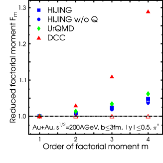
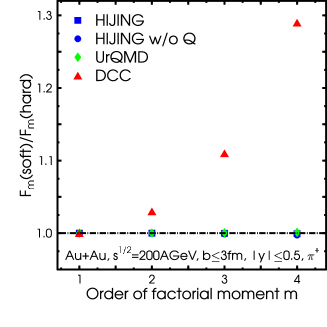
Figure 15: Left: Reduced factorial moments for the multiplicity of positively charged pions emitted at mid rapidity in central $Au+Au$ collisions at the full RHIC energy, as obtained from semi-classical solutions of the linear sigma model in an expanding cylindrical geometry (triangles) [71]. Also shown are the results generated by HIJING with (squares) or without (circles) jet quenching and by UrQMD (diamonds). Solid and open symbols correspond to soft ($p_{T}\leq 200$ MeV) and hard ($p_{T}\geq 200$ MeV) pions respectively. Right: The corresponding ratios of reduced factorial moments calculated for soft and hard pions. From Ref. [117].

It is interesting to compute the reduced factorial moments in a specific model of DCC production. In Ref. [117], Bleicher et al. have performed such an analysis in the context of a semi-classical treatment of the linear sigma model dynamics, in an expanding geometry with cylindrical symmetry [71]: Using the classical field theory methods described in Sec. 2.2, one computes the average occupation number $\bar{n}_{a}({\bf k})$ in a given momentum mode ${\bf k}$ from an expression analogous to Eq. (49), suitably adapted to the expanding geometry. Identifying each classical field configuration with a quantum-mechanical coherent state, the actual multiplicity is then sampled from the associated Poisson distribution with average given by $\bar{n}_{a}({\bf k})$. The latter fluctuates from event to event and one finally performs a statistical average over initial field configurations in a thermal ensemble at a given initial temperature $T_{0}$. The corresponding reduced factorial moments are shown in the left panel of Fig. 15, for both soft ($p_{T}\leq 200$ MeV) and hard ($p_{T}\geq 200$ MeV) pions. Also shown are the corresponding results obtained from the event generators HIJING [118] and UrQMD [119, 120], based on standard production mechanisms. The latter clearly exhibit non-Poissonian fluctuations, with a gentle increase of the reduced factorial moments $F_{i}$ with the order $i$, both for soft and hard pions. In contrast, the dynamics of the linear sigma model leads to reduced factorial moments that remain close to unity for the hard pions while increasing rapidly for the soft pions, indicating enhanced multiplicity fluctuations.

The qualitative difference with standard production mechanisms is better emphasized by considering the ratios between the reduced moments for soft and hard pions, as illustrated in the right panel of Fig. 15. These ratios may provide a useful observable to search for dynamical fluctuations beyond what has been included in standard event generators.

2.4.2 Charged-neutral fluctuations and robust observables

The most striking feature of the coherent (semi-classical) nature of DCC emission is the anomalously large event-by-event fluctuations of the neutral fraction of produced pions, see Eq. (10). This is at the basis of most existing DCC hunt strategies. Similar to the previous analysis of multiplicity, such charged-neutral multiplicity fluctuations can be conveniently studied by means of the bivariate factorial moments

$$\langle{n_{\rm ch}}({n_{\rm ch}}-1)\cdots({n_{\rm ch}}-i+1)\,n_{0}(n_{0}-1)\cdots(n_{0}-j+1)\rangle\,,$$ (125)

where ${n_{\rm ch}}$ and $n_{0}$ denote the charged and neutral-pion multiplicity respectively. Here we review the discussion of charged-neutral fluctuations presented in Ref. [121] for the analysis of the MiniMAX experiment at the Fermilab Tevatron. In particular, these authors have introduced specific observables (see Eq. (142) below) which are rather insensitive to the fluctuations of the total multiplicity and, therefore, essentially probe the charged-to-neutral ratio fluctuations for a wide class of production models. These so-called robust observables are also largely insensitive to detector efficiencies.

Generating functionals for bivariate factorial moments

Let $p({n_{\rm ch}},n_{0})$ denote the probability for the occurrence of ${n_{\rm ch}}$ charged and $n_{0}$ neutral pions in a multi-particle event, in a given region of phase-space. Equivalently, one introduces the generating function:

$$G({z_{\rm ch}},z_{0})=\sum_{{n_{\rm ch}},n_{0}\geq 0}p({n_{\rm ch}},n_{0})\,z_{\rm ch}^{n_{\rm ch}}\,z_{0}^{n_{0}}\,,$$ (126)

which encodes the bivariate factorial moments (125):

$$\Big{<}\frac{{n_{\rm ch}}!}{({n_{\rm ch}}-i)!}\frac{n_{0}!}{(n_{0}-j)!}\Big{>}=\left.\frac{\partial^{i+j}G({z_{\rm ch}},z_{0})}{\partial z_{\rm ch}^{i}\partial z_{0}^{j}}\right|_{{z_{\rm ch}}=z_{0}=1}\,.$$ (127)

Denoting by $P(N)$ the total multiplicity distribution in the considered region of phase-space, one writes

$$p({n_{\rm ch}},n_{0})=P(N)p_{N}({n_{\rm ch}},n_{0})\,,$$ (128)

where $p_{N}({n_{\rm ch}},n_{0})$ denotes the conditional probability that ${n_{\rm ch}}$ of the $N$ produced pions be charged and $n_{0}=N-{n_{\rm ch}}$ be neutral. A wide class of models can be described by the following “binomial transform” [121]:

$$p_{N}({n_{\rm ch}},n_{0})=\frac{N!}{{n_{\rm ch}}!n_{0}!}\int_{0}^{1}df\,p(f)\,f^{n_{0}}(1-f)^{n_{\rm ch}}\,.$$ (129)

For instance, the case of generic pion production can be described by a standard binomial distribution, which corresponds to $p(f)=\delta(f-\bar{f})$, where $\bar{f}=1/3$ is the mean fraction of neutral pions. Equation (129) also includes the case of ideal DCC production, which corresponds to $p(f)=1/2\sqrt{f}$, see Eq. (34). Using Eqs. (126), (128) and (129), one can write:

$$G({z_{\rm ch}},z_{0})=\int_{0}^{1}df\,p(f)\,G(fz_{0}+(1-f){z_{\rm ch}})$$ (130)

where

$$G(z)=\sum_{N\geq 0}P(N)\,z^{N}$$ (131)

is the generating function for the factorial moments of the total multiplicity fluctuations.

Charged-pions–photons fluctuations

Neutral pions are detected through their decay in a pair of photons $\pi^{0}\to\gamma\gamma$. It is, therefore, useful to measure directly the bivariate factorial moments for charged-pions–photons fluctuations. The latter can be defined as in Eq. (125) with the replacement $n_{0}\to n_{\gamma}$, the number of detected photons in the region of momentum-space under consideration, and $\partial/\partial z_{0}\to\partial/\partial z_{\gamma}$. For ideal detection efficiency, the corresponding generating functional can be obtained from Eq. (130) by replacing $z_{0}\to z_{\gamma}^{2}$. More realistically, there are probabilities $\epsilon_{0,1,2}$ that $0$, $1$, or $2$ photons from the $\pi^{0}$ decay be actually detected, with $\epsilon_{0}+\epsilon_{1}+\epsilon_{2}=1$. These three possibilities can be taken into account by introducing the following generating function:

$$g_{0}({z_{\gamma}})=\epsilon_{0}+\epsilon_{1}{z_{\gamma}}+\epsilon_{2}{z_{\rm ch}}^{2}\,.$$ (132)

Similarly, taking into account the detection efficiency for charged pions, there is a probability $\epsilon_{\rm ch}$ that a charged pion be actually observed in the detector and a probability $1-\epsilon_{\rm ch}$ for not observing it. As before, these two possibilities can be described by the following generating function:

$$g_{\rm ch}({z_{\rm ch}})=(1-\epsilon_{\rm ch})+\epsilon_{\rm ch}{z_{\rm ch}}\,.$$ (133)

Thus the relevant generating functional for observed charged-pions–photons fluctuations, taking into account finite detection efficiencies, can be obtained from Eq. (130) with the replacement ${z_{\rm ch}}\to g_{\rm ch}({z_{\rm ch}})$ and $z_{0}\to g_{0}({z_{\gamma}})$ [121]:

$$G_{\rm obs}({z_{\rm ch}},{z_{\gamma}})=G(g_{\rm ch}({z_{\rm ch}}),g_{0}({z_{\gamma}}))\,.$$ (134)

One has, for the observed bivariate moments:

$$\Big{<}\frac{{n_{\rm ch}}!}{({n_{\rm ch}}-i)!}\frac{{n_{\gamma}}!}{({n_{\gamma}}-j)!}\Big{>}_{\rm obs}=\left.\frac{\partial^{i+j}G_{\rm obs}({z_{\rm ch}},{z_{\gamma}})}{\partial z_{\rm ch}^{i}\partial{z_{\gamma}}^{j}}\right|_{{z_{\rm ch}}={z_{\gamma}}=1}\,.$$ (135)

For instance, one easily obtains, for the first moments:

$$\langle{n_{\gamma}}\rangle_{\rm obs} = (\epsilon_{1}+2\epsilon_{2})\,\langle f\rangle\,\langle N\rangle$$ (136)

$$\langle{n_{\rm ch}}\rangle_{\rm obs} = \epsilon_{\rm ch}\,\langle 1-f\rangle\,\langle N\rangle$$ (137)

$$\langle{n_{\gamma}}{n_{\rm ch}}\rangle_{\rm obs} = \epsilon_{\rm ch}(\epsilon_{1}+2\epsilon_{2})\,\langle f(1-f)\rangle\,\langle N(N-1)\rangle$$ (138)

$$\langle{n_{\gamma}}({n_{\gamma}}-1)\rangle_{\rm obs} = (\epsilon_{1}+2\epsilon_{2})^{2}\langle f^{2}\rangle\langle N(N-1)\rangle+2\epsilon_{2}\langle f\rangle\langle N\rangle$$ (139)

$$\langle{n_{\rm ch}}({n_{\rm ch}}-1)\rangle_{\rm obs} = \epsilon_{\rm ch}^{2}\,\langle(1-f)^{2}\rangle\,\langle N(N-1)\rangle\,,$$ (140)

where the brackets on the RHS denote an average with respect either to the multiplicity distribution $P(N)$ or to the distribution $p(f)$ (cf. Eq. (129)).

From the above expressions, one observes that the ratio

$$r_{1,1}=\frac{\langle{n_{\rm ch}}{n_{\gamma}}\rangle_{\rm obs}\langle{n_{\rm ch}}\rangle_{\rm obs}}{\langle{n_{\rm ch}}({n_{\rm ch}}-1)\rangle_{\rm obs}\,\langle{n_{\gamma}}\rangle_{\rm obs}}=2\frac{\langle f(1-f)\rangle}{\langle(1-f)^{2}\rangle}$$ (141)

is independent of the efficiencies introduced above as well as of the multiplicity distribution and only depends on the distribution $p(f)$. More generally, it is easy to check that the following ratios:

$$r_{i,1}=\frac{F_{i,1}}{F_{i+1,0}}\,,$$ (142)

of reduced bivariate factorial moments:

$$F_{i,j}=\frac{\langle{n_{\rm ch}}({n_{\rm ch}}-1)\cdots({n_{\rm ch}}-i+1){n_{\gamma}}({n_{\gamma}}-1)\cdots({n_{\gamma}}-j+1)\rangle_{\rm obs}}{\langle{n_{\rm ch}}\rangle_{\rm obs}^{i}\langle{n_{\gamma}}\rangle_{\rm obs}^{j}}\,.$$ (143)

are robust observables in the above sense:

$$r_{i,1}=2\frac{\langle f(1-f)^{i}\rangle}{\langle(1-f)^{i+1}\rangle}\,.$$ (144)

Moreover, these ratios are sensitive to the difference between generic and DCC production. For generic production, $\langle f^{i}\rangle=\langle f\rangle^{i}=(1/3)^{i}$ and one immediately gets:

$$r_{i,1}({\rm generic})=1$$ (145)

for all $i$’s. In contrast, for ideal DCC production, one has:

$$\langle f^{i}(1-f)^{j}\rangle_{\rm DCC}=\frac{\Gamma(i+\frac{1}{2})\Gamma(j+1)}{2\Gamma(i+j+\frac{3}{2})}\,,$$ (146)

from which one obtains [121]:

$$r_{i,1}({\rm DCC})=\frac{1}{i+1}\,.$$ (147)

The increasing difference between the generic and ideal DCC production mechanisms with increasing order $i$ of the ratios $r_{i,1}$ clearly reflects the broadness of the charged-to-neutral distribution in the latter case.

Mixed events

The above discussion concerns the cases of pure generic versus pure DCC production. More realistic descriptions should include intermediate situations, where both generic and DCC production mechanisms contribute. Various types of such mixed events have been studied in [121]. Here, we consider a model where a DCC is formed with probability $\alpha$ and, when this happens, the detected pions are either of generic or of DCC origin. The corresponding generating function is given by the product:

$$G_{\rm mix}({z_{\rm ch}},z_{0})=G_{\rm DCC}({z_{\rm ch}},z_{0})\,G_{\rm gen}({z_{\rm ch}},z_{0})\,.$$ (148)

where $G_{\rm DCC}({z_{\rm ch}},z_{0})$ is given by the generic form Eqs. (130)-(131) with multiplicity distribution $P_{\rm DCC}(N)$ and with $p_{\rm DCC}(f)=1/2\sqrt{f}$. Similarly, $G_{\rm gen}({z_{\rm ch}},z_{0})$ corresponds to a given multiplicity distribution $P_{\rm gen}(N)$ and $p_{\rm gen}(f)=\delta(f-1/3)$. In the cases where no DCC is formed, which occur with probability $1-\alpha$, the production is purely of generic type. The total generating function takes the form:

$$G({z_{\rm ch}},z_{0})=\alpha G_{\rm mix}({z_{\rm ch}},z_{0})+(1-\alpha)G_{\rm gen}({z_{\rm ch}},z_{0})\,.$$ (149)

From the definitions (142) and (143), and using (127) and (149) above, one can compute the robust ratios $r_{i,1}$ in the present model. For instance, one finds:

$$r_{1,1}=\frac{1+\alpha(A+B)}{1+\alpha(A+2B)}\,,$$ (150)

where

$$A = 2\frac{\langle N\rangle_{\rm DCC}\langle N\rangle_{\rm gen}}{\langle N(N-1)\rangle_{\rm gen}}$$ (151)

$$B = \frac{3}{5}\frac{\langle N(N-1)\rangle_{\rm DCC}}{\langle N(N-1)\rangle_{\rm gen}}\,.$$ (152)

Here, the brackets denote averages with respect to the multiplicity distributions corresponding to either the DCC or the generic production mechanisms, with obvious notations. The case of pure generic production is obviously recovered for $\alpha=0$. Assuming that the probability of DCC formation is small, $\alpha\ll 1$, one obtains the approximate expression:

$$r_{1,1}\approx 1-\frac{3\alpha}{5}\frac{\langle N(N-1)\rangle_{\rm DCC}}{\langle N(N-1)\rangle_{\rm gen}}\,.$$ (153)

Figure 16: The robust ratios $r_{i,1}$ for the model described in the text (cf. Eq. (154)) with, from top to bottom: $i=1,\ldots,5$, as a function of the fraction $\beta$ of DCC pions in the considered region of phase space. The probability that a DCC forms is $\alpha=10^{-3}$. We have assumed that the total multiplicity distributions $P_{\rm gen}(N)$ and $P_{\rm DCC}(N)$ are both Poissonian for simplicity.

Similarly, one can compute the ${\mathcal{O}}(\alpha)$ deviation from pure generic production due to the presence of a DCC for higher-order ratios. One obtains, after some calculations:

$$r_{i,1}\approx 1-\alpha\sum_{k=1}^{i}\frac{i!}{(i-k)!}\,\frac{k\,(3\beta)^{k+1}}{(2k+3)!!}\,\frac{F_{k+1}^{\rm DCC}F_{i-k}^{\rm gen}}{F_{i+1}^{\rm gen}}$$ (154)

where $\beta=\langle N\rangle_{\rm DCC}/\langle N\rangle_{\rm gen}$ is the fraction of DCC pions in the region of phase-space considered and the $F_{j}$’s denote the reduced factorial moments, cf. Eq. (124), corresponding either to the DCC or to the generic multiplicity distributions. As expected, the deviation from $r_{i,1}=1$ is larger for higher-order ratios and increases as the probability of DCC formation and/or as the fraction $\beta$ of DCC pions increase. This is illustrated in Fig. 16, where we show the ratios $r_{i,1}$ for $i=1,\ldots,5$ as a function of $\beta$ for a given value of the probability $\alpha$. For illustration, we have taken both the multiplicity distributions $P_{\rm gen}(N)$ and $P_{\rm DCC}(N)$ to be Poissonian, that is all the reduced factorial moments $F_{j}^{\rm gen}=F_{j}^{\rm DCC}=1$ in (154). This constitute a lower bound on the expected deviation from $1$ for the robust ratios $r_{i,1}$.

The results described here assume the general form (129) for the multiplicity distribution. This includes ideal DCC production as well as simple modelizations of generic production. It would be interesting to extend the analysis of robust ratios to dynamical scenarios of DCC formation, such as e.g. semi-classical simulations of the out-of-equilibrium chiral phase transition, as described in previous sections.

2.4.3 Multi-resolution discrete wavelet analysis

As described above, a possible DCC signal would appear as a localized structure in momentum space. To search for such structure in the lego plot, the authors of Ref. [122] have proposed to use the so-called multi-resolution wavelet analysis. This provides a useful tool to identify possible structures simultaneously in term of their size and location in momentum space. This generalizes the standard Fourier analysis. The technique has been applied to classical simulations of the linear sigma model [122, 124]. It has also been used by various experimental collaborations (see Sec. 3). Here, we review the basics of the discrete wavelet analysis.

To illustrate the method, we consider a one-dimensional phase-space, described by the dimensionless variable $x$ in the interval $[0,1]$. Any observable can be represented by a function $f(x)$ on this interval. Let us cut the accessible phase-space in $2^{j}$ bins of size $\Delta x=1/2^{j}$, where $j$ is a positive integer $j<j_{max}$, with $j_{max}$ corresponding to the finest accessible resolution. To each collision event corresponds a given sample of the function $f(x)$. Call $f^{j}_{k}=f(x=k\Delta x)$ the value of the sampled function in the $k$th bin, the complete sample can be represented by the following function:

$$f^{(j)}(x)=\sum_{k=0}^{2^{j}-1}f_{k}^{j}\,\phi_{k}^{j}(x)$$ (155)

where $\phi_{k}^{j}(x)$ is zero everywhere but in the $k$th bin:

$$\phi^{j}_{k}(x)=\left\{\begin{array}[]{ll}1&k/2^{j}\leq x<(k+1)/2^{j}\\ 0&{\rm otherwise}\end{array}\right.\,.$$ (158)

Notice that the “bin functions” $\phi^{j}_{k}(x)$ can be obtained as translations and dilation of a single function $\phi(x)$, called the mother function:

$$\phi^{j}_{k}(x)=\phi(2^{j}x-k)\,,$$ (159)

where, in the present case, $\phi(x)=\theta(1-x)\theta(x)$.

Equation (155) describes the sampled observable at the resolution scale $j$. To detect structures at lower resolution scales, one can apply the following coarse-graining procedure: Replace two adjacent bins $2k$ and $2k+1$ by a single bin of size $2\Delta x=1/2^{j-1}$, with corresponding bin function given by:

$$\phi^{j-1}_{k}(x)=\phi^{j}_{2k}(x)+\phi^{j}_{2k+1}(x)\,,$$ (160)

and define the value $f^{j-1}_{k}$ of the function in the new bin $k$ as the average of the values in the previous smaller bins:

$$f^{j-1}_{k}=\frac{1}{2}(f^{j}_{2k}+f^{j}_{2k+1})\,.$$ (161)

The resulting coarse-grained sample at scale $j-1$ is simply given by:

$$f^{(j-1)}(x)=\sum_{k=0}^{2^{j-1}-1}f^{j-1}_{k}\,\phi^{j-1}_{k}(x)\,.$$ (162)

Equation (162) defines the mother function representation of the distribution $f(x)$ at scale $j-1$. The $f^{j-1}_{k}$’s are accordingly called the mother function coefficients (MFCs). Clearly the procedure described above eliminates all fluctuations at shorter scales than the resolution scale $j-1$. These steps can be repeated to search for possible structures from the finest experimental resolution scale $j_{max}$ to the lowest one $j=0$.

The information lost at each step in the coarse-graining procedure is encoded in the difference $\tilde{f}^{(j-1)}(x)\equiv f^{(j)}(x)-f^{(j-1)}(x)$. It is easy to show that the latter can be given a similar representation:

$$\tilde{f}^{(j-1)}(x)=\sum_{k=0}^{2^{j-1}-1}\tilde{f}^{j-1}_{k}\,\psi^{j-1}_{k}(x)\,,$$ (163)

where the functions $\psi^{j-1}_{k}$ are given by:

$$\psi^{j-1}_{k}(x)=\phi^{j}_{2k}(x)-\phi^{j}_{2k+1}(x)\,.$$ (164)

They can be obtained as translations and dilations of the so-called father function: $\psi^{j}_{k}(x)=\psi(2^{j}x-k)$, where, in the present case, $\psi(x)=\phi(2x)-\phi(2x-1)$. The corresponding father function coefficients (FFCs) in (163) are related to the MFCs at the previous resolution scale $j$ through:

$$\tilde{f}^{j-1}_{k}=\frac{1}{2}(f^{j}_{2k}-f^{j}_{2k+1})\,.$$ (165)

Equation (163) defines the father function representation of the sampled distribution $f(x)$ at the scale $j-1$. Clearly, the FFCs (165) at a given scale $j$ measure the variation of the sampled distribution $f$ between two adjacent bins. The information about the size of the fluctuations at each scale can be conveniently encoded in the following power spectrum:

$$P_{j}=\frac{1}{2^{j}}\sum_{k=0}^{2^{j}-1}|\tilde{f}^{j}_{k}|^{2}\,.$$ (166)

Similar to the Parseval theorem for the Fourier transform, one has:

$$\sum_{j\geq 0}P_{j}=\int_{0}^{1}dx\,|f(x)|^{2}\,.$$ (167)

Figure 17: Scale dependence of the discrete wavelet power spectrum for various dynamically generated data. From Ref. [122].

To demonstrate the method, the authors of [122] have applied the above analysis to various dynamically generated data. They have considered the evolution of the pion field as described by the linear sigma model in the Hartree approximation, for a boost invariant $1+1$ expanding geometry. The initial field configurations are sampled from the quenched ensemble described in Sec. 2.2.1. The discrete wavelet analysis is applied to the ratio:

$$h(\eta)=\frac{\pi_{3}^{2}(\eta)}{\pi_{1}^{2}(\eta)+\pi_{2}^{2}(\eta)+\pi_{3}^{2}(\eta)}\,,$$ (168)

where $\pi_{1,2,3}(\eta)$ are the isospin Cartesian components of the pion field as a function of the spatial rapidity $\eta=\frac{1}{2}\ln(t+z)/(t-z)$, where $z$ is the collision axis. The ratio (168) is related to the neutral pion fraction discussed in previous sections. The rapidity-interval $-\eta_{max}<\eta<\eta_{max}$, with $\eta_{max}=5$, is bined with a bin size $\Delta\eta=0.08$, corresponding to a finest resolution scale $j_{max}=7$, such that $2\eta_{\max}/\Delta\eta=2^{j_{max}}$. Figure 17 shows the corresponding power spectrum (167) at various scales, for both the initial quenched ensemble (random sample) and the final time evolved ensemble (DCC sample). Also shown are the results corresponding to a thermal ensemble as well as the power spectrum obtained from HIJING Monte Carlo data. The DCC sample clearly exhibit a non-trivial structure, reflecting clustering in spatial rapidity. Similar results have been obtained in Ref. [124] for three-dimensional classical simulations of the linear sigma model in a static geometry with a cooling term, as described in subsection 2.2.2 above.

It is important to mention that the analysis of Refs. [122, 124] concerns data sampled in coordinate space. Although this is sufficient to demonstrate the wavelet analysis technique, it would be of interest, for phenomenological purposes, to perform similar analysis in momentum space.

2.4.4 Electromagnetic signatures

Because they interact strongly with the background of other hadrons, hadronic signals may rapidly loose the information they carry before they leave the interaction region. In contrast, electromagnetic signals do not undergo multiple rescatterings and, therefore, provide a sensitive probe of the various stages of the collision. If the DCC lives long enough, they might probe its formation even if the latter is diluted in the hadronic environment before freeze-out.

It has been proposed that anomalous pion production from a DCC would result in anomalous radiation of low-momentum photon and/or low-mass dileptons [125, 126, 127, 128, 129]. Here we illustrate these ideas in the case of dilepton production. At lowest order in the electromagnetic coupling constant $\alpha_{\rm em}$, the dilepton production rate reads:

$$\frac{dN_{\ell^{+}\ell^{-}}}{d^{4}q}=\frac{\alpha_{\rm em}^{2}}{6\pi^{3}}\frac{B(q^{2})}{q^{4}}(q^{\mu}q^{\nu}-q^{2}g^{\mu\nu})\,W_{\mu\nu}(q)\,,$$ (169)

where $q^{\mu}$ is the four-momentum of the lepton pair, such that $q^{2}\geq 4m_{\ell}^{2}$, with $m_{\ell}$ the lepton mass, $B(q^{2})=(1+2m_{\ell}^{2}/q^{2})(1-4m_{\ell}^{2}/q^{2})^{1/2}$ and $W^{\mu\nu}(q)$ is the $4$-dimensional Fourier transform of the electromagnetic current correlator:

$$W^{\mu\nu}(q)=\int d^{4}xd^{4}y\,{\rm e}^{-iq\cdot(x-y)}\langle J^{\mu}(x)J^{\nu}(y)\rangle\,,$$ (170)

where the brackets represent the average in the state under consideration. and $J^{\mu}(x)$ is the electromagnetic current operator:

$$J^{\mu}(x)=\frac{i}{2}[\pi^{\dagger}(x)\stackrel{{\scriptstyle\leftrightarrow}}{{\partial^{\mu}}}\pi(x)-\pi(x)\stackrel{{\scriptstyle\leftrightarrow}}{{\partial^{\mu}}}\pi^{\dagger}(x)]\,,$$ (171)

where $f\!\!\stackrel{{\scriptstyle\leftrightarrow}}{{\partial_{\mu}}}\!\!g=f\partial_{\mu}g-(\partial_{\mu}f)g$ and where $\pi(x)$ and $\pi^{\dagger}(x)$ denote the charged pion field operators.

To illustrate the anomalous electromagnetic emission due to a DCC, we essentially follow the schematic model presented in [126, 127]. The presence of a DCC may be modeled by splitting the pion field operators into a classical part $\pi_{\rm cl}(x)$, which represent the coherent DCC excitation, and the rest $\tilde{\pi}(x)$, which describes the background pions:

$$\pi(x)=\pi_{\rm cl}(x)+\tilde{\pi}(x)$$ (172)

The electromagnetic current (171) can be written as a sum of three contributions:

$$J^{\mu}(x)=J^{\mu}_{\rm cl}(x)+J^{\mu}_{1}(x)+J^{\mu}_{2}(x)\,,$$ (173)

where $J^{\mu}_{\rm cl}(x)$ is the purely classical contribution, obtained from Eq. (171) with the replacement $\pi\to\pi_{\rm cl}$, and $J^{\mu}_{n=1,2}(x)$ contains $n=1,2$ powers of the field $\tilde{\pi}$ respectively. Inserting this decomposition in Eq. (170) and assuming that the system of background pions is electrically neutral, one obtains:

$$W^{\mu\nu}(q)=W^{\mu\nu}_{\rm cl}(q)+W^{\mu\nu}_{1}(q)+W^{\mu\nu}_{2}(q)\,,$$ (174)

where the first term on the RHS,

$$W^{\mu\nu}_{\rm cl}(q)=J^{\mu}_{\rm cl}(q)\,J^{\nu*}_{\rm cl}(q)$$ (175)

describes the purely classical contribution and

$$W^{\mu\nu}_{n}(q)=\langle J^{\mu}_{n}(q)\,J^{\nu\dagger}_{n}(q)\rangle\,,$$ (176)

with $J^{\mu}_{\rm cl}(q)$ and $J^{\mu}_{n}(q)$ the four-dimensional Fourier transform of $J^{\mu}_{\rm cl}(x)$ and $J^{\mu}_{n}(x)$ respectively.

The contribution to the rate (169) from the first term on the RHS on Eq. (174) corresponds to the anomalous bremsstrahlung from the DCC itself. As an illustrative example [126], it can be estimated using the Blaizot-Krzywicki classical solution [2], described in Sec. 2.1. For this purpose, it is useful to notice that the electromagnetic current (171) actually coincides with the third component of the iso-vector current ${\vec{V}}^{\mu}={\vec{\pi}}\times\partial^{\mu}{\vec{\pi}}$:

$$J^{\mu}(x)=\pi_{1}(x)\partial^{\mu}\pi_{2}(x)-\pi_{2}(x)\partial^{\mu}\pi_{1}(x)=V^{\mu}_{3}(x)\,.$$ (177)

For the one-dimensional boost-invariant solution of Refs. [2, 42], one has ${\vec{\pi}}(x)\equiv{\vec{\pi}}(\tau)$, with proper-time $\tau=\sqrt{t^{2}-z^{2}}$, and the classical iso-vector current can be written as (cf. (15)):

$${\vec{V}}^{\mu}_{\rm cl}(x)=u^{\mu}\frac{{\vec{a}}}{\tau}\,\theta(\tau-\tau_{0})\,g({\bf x}_{\perp})$$ (178)

where $u^{\mu}=(\cosh\eta,\sinh\eta,0,0)$, with spatial rapidity $\eta$ defined as $\tanh\eta=z/t$. Here, following the authors of Ref. [126], we have multiplied the boost-invariant solution of Blaizot and Krzywicki by a slowly varying function of the transverse coordinates $g({\bf x}_{\perp})$ to account for the finite transverse extent of the system. The Fourier transform of the current (178) is easily evaluated and one obtains, after averaging over the possible orientations of the iso-vector ${\vec{a}}$ [126]:

$$\frac{dN_{\ell^{+}\ell^{-}}^{\rm cl}}{dydMd^{2}q_{\perp}}=\frac{\alpha_{\rm em}^{2}}{24\pi}\langle a_{3}^{2}\rangle\,\frac{q_{\perp}^{2}B(M^{2})}{M_{\perp}^{2}\,M^{3}}\,[J_{0}^{2}(M_{\perp}\tau_{0})+N_{0}^{2}(M_{\perp}\tau_{0})]\,|\tilde{g}({\bf q}_{\perp})|^{2}\,,$$ (179)

where $M=\sqrt{q^{2}}$ is the invariant mass of the lepton pair, $y$ and ${\bf q}_{\perp}$ its longitudinal rapidity and transverse momentum respectively, and $M_{\perp}\equiv\sqrt{q_{\perp}^{2}+M^{2}}$. Here, $J_{0}$ and $N_{0}$ are usual Bessel functions and $\tilde{g}({\bf q}_{\perp})$ is the Fourier transform in transverse space of the shape function $g({\bf x}_{\perp})$. High transverse momentum dilepton are suppressed due to the finite transverse extent of the source. For instance, for a Gaussian shape $g({\bf x}_{\perp})=\exp(-x_{\perp}^{2}/R_{\perp}^{2})$, one has a strong exponential suppression: $|\tilde{g}({\bf q}_{\perp})|^{2}\propto\exp(-q_{\perp}^{2}R_{\perp}^{2}/2)$. Notice that, as a consequence of boost-invariance in the present model, the rate (179) does not depend on the dilepton rapidity $y$. Finally, $\langle a_{3}^{2}\rangle$ measures the fluctuations of the strength of the iso-vector current in the initial state. Neglecting the pion mass, The latter can be related to the mean initial energy density $\langle\epsilon_{0}\rangle$ using Eq. (22). Assuming a high temperature symmetric initial state where the values of the fields $({\vec{\pi}},\sigma)$ and their proper-time derivatives at $\tau=\tau_{0}$ are Gaussian random numbers of zero mean and of variance $\sigma_{1}$ and $\sigma_{2}$ respectively, as in (25), one obtains:

$$\langle a_{3}^{2}\rangle=2\kappa_{0}^{2}=\frac{\tau_{0}^{2}}{3}\langle\epsilon_{0}\rangle\,.$$ (180)

with $\kappa_{0}=\sigma_{1}\sigma_{2}\tau_{0}$.

The dependence of the yield (179) on the dilepton mass at fixed transverse momentum is shown by the dotted curve in Fig. 18. Also shown are the contributions from the annihilations of on-shell background pions, assuming that the latter form a thermal bath (dashed curve), as well as the contribution arising from the interactions between thermal and DCC pions as described below (dot-dashed curve). One observes that the bremsstrahlung contribution (179) from off-shell DCC pions have no threshold and is actually mainly concentrated at low invariant mass $M\lesssim 2m_{\pi}$. In this region, however, the yield is extremely sensitive to the initial time $\tau_{0}$ due to the singular behavior of Bessel Neumann function $N_{0}(z)$. Moreover, this signal would probably be very difficult to discriminate in a heavy-ion collision due to the large background from Dalitz decays $\pi^{0}\to e^{+}e^{-}\gamma$ in this kinematical region (see e.g. [130]).

Figure 18: The $e^{+}e^{-}$ yield (169) as a function of the dilepton invariant mass. The dotted line corresponds to the anomalous bremsstrahlung from the DCC classical field configuration; The dashed line represents the contribution from the surrounding thermal bath at temperature $T$; Finally, the dot-dashed curve represents the contribution arising from the interactions between DCC and thermal pions. The relevant parameters (see text) are: $T=145$ MeV, $\langle\epsilon_{0}\rangle=58$ MeV/fm³, $\tau_{0}=1$ fm. The absolute normalization of the DCC contribution depends on the details of the shape function $g({\bf x}_{\perp})$ for the DCC and is given here for a Gaussian shape $g({\bf x}_{\perp})=\exp(-x_{\perp}^{2}/R_{\perp}^{2})$ with $R_{\perp}=2$ fm. The relative normalization of the various contributions are not realistic (see text). From Ref. [127].

Another possibility, suggested in Ref. [127], is that non-coherent pions from the surrounding heat bath may annihilate on the coherent DCC state, forming dilepton pairs of typical invariant masses in a rather narrow window around $M\simeq 2m_{\pi}$, thus avoiding the $\pi^{0}$ Dalitz-decay region. The corresponding contribution to the dilepton rate (169) comes from the second term on the RHS side of Eq. (174). Assuming a thermal bath of non-interacting pions at temperature $T$, one obtains, after some calculations, the following contribution [127]:

$$\frac{dN^{(1)}_{\ell^{+}\ell^{-}}}{dydMd^{2}q_{\perp}} = \frac{2\alpha_{\rm em}^{2}}{3\pi^{3}}\frac{1}{M}\int\frac{d^{3}k}{2\omega_{k}(2\pi)^{3}}\left[\frac{(k\cdot q)^{2}}{M^{2}}-m_{\pi}^{2}\right]$$ (181)

$$\left\{(1+n^{-}_{k})\,|\pi_{\rm cl}(r)|^{2}+(1+n^{+}_{k})\,|\pi_{\rm cl}(-r)|^{2}\right.$$

$$\,\,+\left.n^{-}_{k}\,|\pi_{\rm cl}(l)|^{2}+n^{+}_{k}\,|\pi_{\rm cl}(-l)|^{2}\right\}.$$

where $\omega_{k}=\sqrt{k^{2}+m_{\pi}^{2}}$, $k^{\mu}=(\omega_{k},{\bf k})$, $r^{\mu}=(k+q)^{\mu}$, $l^{\mu}=(k-q)^{\mu}$ and $n_{k}^{\pm}$ denotes the equilibrium Bose-Einstein distribution at temperature $T$ for positive and negative pions. The first two terms in curved brackets on the RHS of (181) correspond to the decay of the classical DCC field into an on-shell thermal pion and a dilepton pair: $\pi_{\rm cl}\to\tilde{\pi}\ell^{+}\ell^{-}$, whereas the last two terms represent the annihilation of a DCC pion against a thermal one: $\pi_{\rm cl}\tilde{\pi}\to\ell^{+}\ell^{-}$. The latter contribution has a threshold at $M=2m_{\pi}$, and produces an enhancement of the dilepton yield around $M\simeq 2m_{\pi}$, as is clearly visible on Fig. 18. A more detailed analysis has been performed in Ref. [127], using classical field dynamics, which indicates that this enhancement is restricted to dilpeton momenta $|{\bf q}|\lesssim 300-500$ MeV.

We would like to stress that Fig. 18 is only meant here to illustrate the dependence of the various contributions to the dilepton yield with the dilepton mass. The relative normalization of the various contributions should not be taken too seriously as it is most probably far from realistic. First, because the present model completely neglects the small probability that a DCC actually forms. In a more realistic description, the rates (179) and (181) should be accordingly rescaled. Second, because the parameters used here correspond to an unexpectedly large contribution from the DCC. Indeed, as a rough estimate of the energy density of the background thermal pion gas, one may use the Stefan-Boltzmann law for a gas of non-interacting massless pions: $\epsilon_{\pi}=g(\pi^{2}/30)T^{4}$ with $g=3$ the pion degeneracy. For $T=145$ MeV used in Fig. 18, one obtains $\epsilon_{\pi}\approx 55$ MeV/fm³ which is similar in magnitude as the initial energy density of the DCC state in the above calculation: $\langle\epsilon_{0}\rangle=58$ MeV/fm³. This is certainly unrealistic, at least in the context of the non-equilibrium chiral phase transition scenario discussed in earlier sections. In a more realistic situations, one expects $\langle\epsilon_{0}\rangle\ll\epsilon_{\pi}$ and the various contributions to the dilepton rate shown in Fig. 18 should be appropriately rescaled.

Finally, we mention that the generic dilepton spectrum in this region is dominated by $\eta$ Dalitz-decays, thus making the measurement of dileptons from a DCC a very difficult task. The possibility of such a measurement would certainly require making appropriate cut on the data, probably in correlation with other hadronic observables. This certainly deserves further investigations.

2.4.5 Further speculations

It is usually believed that, in the context of high-energy nuclear collisions, the best place for DCC searches is the central rapidity region of the most central collisions, because this is where one expects the deposited energy density to be the highest, thereby providing the most favorable conditions for chiral symmetry restoration. However, as we have seen previously, this is also a place where DCC signatures might be difficult to observe. Here, we briefly mention alternative suggestions.

Rajagopal has argued in Ref. [131] that semi-peripheral collisions at RHIC energies might provide more favorable conditions for efficient quenching as well as sooner freeze-out, hence a better chance that DCC pions be visible in the detectors. Another interesting motivation for looking at such collision events has been proposed by the authors of Ref. [132, 99], who argued that strong electromagnetic fields could result in a coherent excitation of the $\pi_{0}$ field through the chiral $U(1)$ anomaly. Such an excitation could be subsequently amplified by the quench mechanism, as discussed at length in the present report. More peripheral collisions might also be interesting for DCC searches because they essentially consists in the collision of the pion clouds of the respective nuclei. The relevant dynamics is, therefore, that of low-energy pion fields and the corresponding physical picture might be closer to the original baked-Alaska scenario (see Sec. 2.1). One could further imagine to favor a particular isospin direction by colliding asymmetric (e.g. neutron rich) nuclei.

Another place of special interest to look for DCC signatures is the projectile or target fragmentation region of nuclear collisions, as advocated by Bjorken [133, 134]. The basic idea is that, viewing the collision in the rest frame of one of the ions, the projectile traverses the target at essentially the speed of light and ejects all the resting nuclear matter away almost instantaneously. If the smoking ruins left behind relax sufficiently slowly toward ordinary vacuum, the relevant dynamics should be that of soft pion fields and relaxation process should be characterized by low-momentum pion emission.

It is also important to stress that present theoretical calculations in the context of the quench scenario in heavy-ion collisions indicate that the DCC might actually be more difficult to observe than originally thought [96, 94, 95, 97, 27] (see subsection 2.2.5). In particular, the results of Ref. [97] suggest that one should try to isolate as much as possible the various Fourier modes of the DCC pion field. Multi-resolution analysis techniques such as the discrete wavelets described above provide very efficient tools for such task. Moreover, in regards to the rather small expected probability that a DCC forms, it would be desirable to perform appropriate cuts on the data sample. For instance, one could restrict the analysis to events with a particularly large pion multiplicity, say larger than the average, in a given region of momentum space. We shall discuss such type of analysis in the experimental part of this review.

Finally, we mention that a number of other observables, which we have not described here, have been discussed in the literature. This includes e.g. non-trivial charged-pion fluctuations [135] – which present the advantage that one does not have to reconstruct the $\pi_{0}$’s, or anomalous strangeness production [61, 136], etc.

3 Experiment

3.1 DCC-search experiments

Can a DCC domain be produced in actual hadron or heavy-ion collisions and, if so, are we capable of detecting them? In the search for the answers to these questions, several experiments have been carried out and some have been planned for future. Some of them are based on the study of cosmic ray showers and others are accelerator-based. The list of all these experiments is given in Table 1. Below we discuss some of these experiments and their capability to look for DCC in terms of measurement of right observables. The results from these experiments will be discussed in detail in Sec. 3.4.

Table 1: Experiments related to search for disoriented chiral condensates.

Year	Type	Experiment	$\sqrt{s}$	Observable
1972-80	Cosmic Ray, Balloons	JACEE [6]	$\geq$ 1.7 TeV	No. of $\gamma$ & $ch$ in 5 $\leq$ $\eta$ $\leq$ 9
1980	Cosmic Ray,	Brazil-Japan	$\geq$ 1.7 TeV	No. of $\gamma$ & $ch$ in
	Mt. Chacaltaya & Fuji			forward $\eta$
1977-91	Cosmic Ray, Mt. Pamir	PAMIR [7]	$\geq$ 1.7 TeV	No. of $\gamma$ & $ch$ in forward $\eta$
1982	Accelerator based,	UA5 [14, 15]	540 GeV	No. of $\gamma$ & $ch$ in $\sim$ 4$\pi$
and	nucleon-nucleon		and	& asymmetry in electro-
1986	collision at CERN		900 GeV	magnetic & hadronic energy
1983	Accelerator based,	UA1 [13]	540 GeV	asymmetry in electromagnetic
	nucleon-nucleon			& hadronic energy
	collision at CERN			in -3.0 $\leq$ $\eta$ $\leq$ 3.0
1996	Accelerator based,	D0	1.8 TeV	asymmetry in electromagnetic
	nucleon-nucleon	and		& hadronic energy
	collision at FERMILAB	CDF [16]		in -4.0 $\leq$ $\eta$ $\leq$ 4.0
1997	- do -	MiniMAX [17]	1.8 TeV	No. of $\gamma$ & $ch$ in
				3.2 $\leq$ $\eta$ $\leq$ 4.2
1998	Accelerator based,	WA98 [18, 20, 21]	17.3 GeV/n	No. of $\gamma$ & $ch$ in
and	nucleus-nucleus			2.9 $\leq$ $\eta$ $\leq$ 3.75
2001	collision at CERN
1999	- do -	NA49 [19]	17.3 GeV/n	$p_{T}$ fluctuation in charged
				particles in 4.0 $\leq$ $\eta$ $\leq$ 5.5
2001	Accelerator based,	PHENIX [22]	200 GeV/n	No. of $\gamma$ & $ch$ in
and	nucleus-nucleus			-0.35 $\leq$ $\eta$ $\leq$ 0.35
2002	collision at RHIC

3.1.1 Cosmic ray experiments

Cosmic ray experiments were performed by exposing stacks of nuclear emulsion chambers at high mountain tops or sending them to high altitudes in balloons. They recorded secondary particles (mostly pions and gamma rays) originating in the successive interactions of a particle of primary cosmic radiation (such as proton) with atmospheric nuclei. The primary cosmic ray particle energies are in the range of $100$ TeV to $10000$ TeV [6]. A cosmic ray event can therefore be thought of as a result of collision between a projectile nucleon of an estimated energy of about 1500 TeV (equivalent center of mass energy $\sqrt{s}\geq~{}1700$ GeV) and an atmospheric nuclei [15]. The mountain top experiments, carried out at Mt. Chacaltaya in Bolivia, at Pamir in Russia and Mt. Fuji in Japan, reported events having large number of charged hadrons (about 63 - 90) and very few or no photons. These events are known as “Centauro-type” events. The first Centauro-type event called “Centauro-I” was reported in 1972. The JACEE collaboration [6], which had sent emulsion chambers in balloons to high altitudes also observed events having anomalously high number of gammas in comparison to charged secondaries. Such events are called “anti-Centauro-type” events. One such interesting event reported by the JACEE collaboration [6] is shown in Fig. 19, where the distributions of charged particles and gammas are presented in $\eta-\phi$ space. One of the possible explanations for these peculiar events with large isospin fluctuations in cosmic ray experiments is the possibile production of a DCC in high-energy collisions.

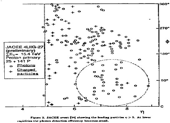
Figure 19: The $\eta-\phi$ phase space distribution of an event from the JACEE collaboration [6]. The region indicated by the circle shows a region with anomalously high ratio of gammas to charged secondaries, called as anti-Centauro event.

There has been critical reviews of the exotic characteristics of Centauro-I. In Refs.  [137, 138] the authors found that there is no original correspondence between the clusters in upper and lower chambers of the emulsion chamber experiment. The authors of Ref. [137] claim that such an event no longer required any new physics to describe the event structure. In Ref. [138] there is a suggestion that the event structure may have arisen due a bundle of target interactions. They however claim that the characteristics, like hadrons not accompained by any $\gamma$ rays, can still not be understood and are very different from commonly observed cosmic ray events.

Recent results from a systematic study of the neutral pion fraction distribution (using sensitive techniques developed for DCC search) in high-energy cosmic ray families detected at high altitudes at Pamir [7] do not exclude such a possibility. The Pamir experiment took data by exposing thick lead chambers of homogeneous structure at Pamir in 1977-1991. The chamber thickness was between 40 - 110 cm Pb and, hence, had a detection probability of $\gamma$-hadron families close to 1. One of the limitations of cosmic ray experiments is that, because of the high energy detection threshold in experiments with emulsion chambers, the investigation of high-energy interaction is limited to the projectile particle fragmentation region. The situation is opposite to that in collider experiments where secondary particles emitted with small angles in far forward regions of the collision cannot be detected because of the beam pipe.

3.1.2 Nucleon-Nucleon collisions

The observation of Centauro-type events motivated experimentalists to look for such events in accelerator-based experiments, even before the concept of the DCC came into picture. The UA1 experiment [13] searched for events having characteristics of cosmic ray Centauros in $p-\bar{p}$ collisions at $\sqrt{s}=540$ GeV, using information on charged particle multiplicities, transverse momenta and the criteria of large hadronic and low electromagnetic energy content in calorimeters. The central image chamber detector of the UA1 apparatus was used to get charged particle tracks. Momenta were obtained from the curvature of the tracks in uniform magnetic field of 0.56 Tesla. The energy information was obtained from layers of finely divided sheets of lead and plastic scintillators which formed the electromagnetic calorimeter. The calorimeter surrounded the central detector. The electromagnetic energy deposition was measured from the first 4 radiation length of material. The hadronic energy contribution was estimated from the rest of the electromagnetic calorimeter and from energy deposition in the iron scintillator calorimeter behind it. No Centauro-like events were seen out of a total data sample of 48K events. Based on this the UA1 collaboration reported an upper limit for the production cross section of the order of a micro-barn for a Centauro events at collider energies equivalent to 155 TeV incident energy on stationary nuclei.

The UA5 experiment [14, 15], through an analysis of 3600 minimum bias events for correlation between photon and charged-particle multiplicities, reported no events having features corresponding to the Centauro events as observed in cosmic-ray emulsion chambers. The detector used for charged particle measurement was a streamer chamber, with a coverage of almost the entire 4$\pi$ solid angle. The photon measurements were based on electromagnetic showers resulting from photons converting through the walls of the vacuum chamber (0.05 to 2.6 radiation length of material) situated between the two streamer chambers. The search were carried out at $\sqrt{s}$ energies of 540 GeV and 900 GeV without any success. The search was extended to high $\sqrt{s}$ energy of 1.8 TeV in the D0 and CDF [16] experiments at Fermilab. These experiments used the technique of the asymmetry in hadronic to electromagnetic energies for DCC search. They also reported null results.

Subsequently a dedicated experiment at Fermilab Tevatron, called MiniMAX [17], was designed by Bjorken, Kowalsky, Taylor and collaborators to look for DCC signals in the far forward rapidity region of $p-\bar{p}$ collisions at $\sqrt{s}=1.8$ TeV. This experiment, located at the C0 area of the Fermilab Tevatron was designed to measure the ratio of charged-to-neutral pions. The acceptance in the lego space of pseudo-rapidity $\eta$ and azimuthal angle $\phi$ is roughly a circle of radius $0.65$ centered at $\eta=4.1$. The MiniMAX apparatus included Multi-Wire Proportional Chambers (MWPC) to measure charged particles, movable 1 radiation length ($X_{0}$) Pb converter to improve the resolution of charged-particles, a trigger scintillator, an array of 28 lead-scintillators acting as electromagnetic calorimeter located behind the MWPC to measure photons and upstream tagging detectors. The analysis of the data with about $8\times 10^{6}$ events was done using the technique of robust observables, discussed earlier in Sec. 2.4, to take care of the small acceptance of the detector and various efficiency factors. The analysis yielded results consistent with no DCC production.

3.1.3 Nucleus-Nucleus collisions

Various DCC searches have also been pursued in high-energy heavy-ion collision experiments. This is motivated by the high energy density and temperature achieved in such collisions, which provide favorable conditions for the DCC production scenario based on the non-equilibrium chiral phase transition [10], as discussed in Sec. 2.2. Among the various heavy-ion experiments, WA98 was the first one which had the capability of measuring photon and charged particle multiplicities over a common region of phase-space, which is a key ingredient for DCC search through neutral fraction fluctuations [20, 18]. The data analyzed by the WA98 collaboration were taken with the $158$ AGeV Pb beam of the CERN SPS on a Pb target of $213~{}\mu$m thickness during a period of WA98 operation without magnetic field. The analysis makes use of a subset of detectors of the WA98 experiment which were used to measure the multiplicities of charged particles and photons. Charged-particle hits ($N_{\mathrm{c}h}$) were counted using a circular Silicon Pad Multiplicity Detector (SPMD) located $32.8$ cm downstream from the target. It provided uniform pseudo-rapidity coverage in the region $2.35<\eta<3.75$. The photon multiplicity was measured using a preshower Photon Multiplicity Detector (PMD) placed $21.5$ m downstream of the target and covering the pseudo-rapidity range $2.9<\eta<4.2$. It consisted of an array of $53,200$ plastic scintillator pads placed behind $3X_{0}$ thick lead converter plates. Clusters of hit pads having total energy deposit above a hadron rejection threshold are identified as “photon-like”. For the DCC analysis the pseudo-rapidity region of common coverage of the SPMD and PMD was selected ($2.9<\eta<3.75$) by WA98 collaboration. The acceptance in terms of transverse momentum extends down to $p_{T}=30$ MeV/c, although no explicit $p_{T}$-selection was applied. As far as analysis goes, there has been a global search of DCC formation  [18] in the WA98 experiment. Asymmetry in $N_{\gamma}$ to $N_{ch}$ ratio over the full common phase space of the photon and charged particle detectors was used to get some idea regarding DCC formation in Pb-Pb collisions at $158$ AGeV. Following the theoretical expectations [1, 2, 10] that the isospin fluctuations, caused by formation of DCC, may produce clusters of coherent pions in phase space forming localized domains, the WA98 collaboration has also searched for localized domains of DCC [20, 21]. This was done by trying to detect large and localized fluctuations in the ratio of photons–to–charged-particles numbers.

An analysis using the momentum information of charged particles without looking at photons was carried out by the NA49 experiment [19] at the CERN SPS to look for DCC. There, particles were selected that had a measured track length of more than $2$ m in one of the two Main Time Projection Chambers (MTPC) outside the magnetic field and were also observed in at least one of the Vertex TPCs inside the superconducting magnets. The NA49 collaboration studied particles in the region: $0.005<p_{T}<1.5$ GeV/c in transverse momentum and $4<y_{\pi}<5.5$ in rapidity. Both the WA98 and NA49 experiments reported results in terms of upper limit on the frequency of DCC formation.

At the RHIC, the STAR experiment [23] plans to look for DCC formation using the combination of photon-multiplicity detector (PMD) and the electromagnetic calorimeter (EMCAL) for photon detection along with the time projection chamber (TPC) and forward-time projection chamber (FTPC) for charged-particle detection [23]. The PHENIX collaboration [22] has also demonstrated its capability to study isospin fluctuations, essentially through charged-particle measurements using drift and pad chambers and photon measurements from the electromagnetic calorimeter of the PHENIX detector [22]. Finally, we mention that the ALICE experiment [24] at the upcoming LHC at CERN will have the combination of a PMD and a charged-particle multiplicity detector (FMD) in the forward rapidity region as well as an electromagnetic calorimeter (PHOS) and a time projection chamber (TPC) near mid-rapidity, which allow for DCC search in different rapidity regions.

3.2 Simulated DCC events

It is important to model DCC pion production in realistic heavy ion collision event generators in order to study the sensitivity of the various techniques developed to look for DCC-like fluctuations in experimental data. This is also useful to get a clear idea of the limitations of both the experiments and the analysis tools at hand. Finally this provides a basis to interpret actual data, as done e.g. by the WA98 [20, 18] and NA49 [19] collaborations. Here, we present a simple model proposed in Refs. [18, 139], where the generic particle production is governed by the VENUS event generator [140] and the DCC pions are introduced by hand at the freeze-out stage. The goal is to observe the effect of DCC domains on measured quantities, assuming DCC pions survive till the freeze-out time. As discussed previously in Sec. 2.3, this assumption is justified by theoretical calculations [101]. The main features of the model are the following:

• DCC-type fluctuations:
  For DCC simulation in a given domain, the identity of charged pions taken pairwise ($\pi^{+}\pi^{-}$) is changed to neutral ones ($\pi^{0}\pi^{0}$) and vice-versa [18, 139], according to the ideal DCC inverse square-root law, Eq. (10).
  

• Domain size:
  The size of a domain is defined in terms of its extent in pseudo-rapidity ($\eta$) and azimuthal angle ($\phi$). In most analysis described in the following, one choses a domain-size of one unit in rapidity: $\Delta\eta=1$ and a variable extent $\Delta\phi$ in azimuthal angle. This is not a bad assumption as it is expected that DCC doamins will occur in small regions and will mostly modify the production of low momentum pions. The influence of DCC on the charge-neutral pion ratio may then be limited to localized $\eta$-$\phi$ regions due to the motion of the DCC domain within the overall collective motion or strong radial flow in heavy ion collisions.

• Number and $p_{T}$ spectrum of DCC pions:
  For simplicity all the pions inside a chosen domain are considered to be DCC-type. As already emphasized, theoretical calculations suggest that DCC pions have low $p_{T}$. In order to study the usefulness of $p_{T}$ information of particles, as discussed in Sec. 3.5 below, one typically consider two cases [141]: (i) all pions with $p_{T}\leq 150$ MeV are taken as DCC pions in a given domain; (ii) a variable number (depending on the domain size) of DCC-pions with $p_{T}\leq 150$ MeV are added by hand to the generic sample of pions in a given domain. The number of these additional pions depends on the size and energy density of the DCC domain. Domains of typical radius $R\sim 3-4$ fm are expected from numerical simulations of the non-equilibrium chiral phase transition in the context of heavy-ion collisions [96, 65, 142]. Assuming the energy density $\epsilon_{\rm DCC}$ of the DCC domain to be about $50$ MeV/fm³, the number of DCC pions is estimated from the relation $\frac{4}{3}\pi R^{3}(\epsilon_{\rm DCC}/m_{\pi})$ to be between $40$ and $100$. This probably gives a reasonable upper bound on actual numbers to be expected.
  

• $\pi^{0}$ decay and photon fraction:
  After introducing DCC-type fluctuations the $\pi^{0}$’s are allowed to decay. The neutral pion fraction $f$ then gets approximately modified to:

  $$f\approx f^{\prime}=\frac{{N_{\gamma}}/2}{{N_{\gamma}}/2+{N_{\rm ch}}}\,,$$ (182)

  where ${N_{\gamma}}$ is the photon multiplicity and ${N_{\rm ch}}$ is the total multiplicity of charged pions.
  

• Percentage of events being DCC-type:
  The sets of events with DCC will be referred to as “nDCC” events. The ensemble of nDCC events may or may not have all the events of DCC type and the percentage $\alpha$ of DCC-type events in a given ensemble can be varied to study the sensitivity of various physical and detector related effect to the observation of DCC.

In order to understand the various techniques used for DCC search, one can apply them to “realistic” simulated DCC events as described above. For this, one assumes [143] a single DCC domain lying within the common pseudo-rapidity coverage of two hypothetical multiplicity detectors for photon and charged particles. To simulate what happens in a true experimental situation, it is necessary to include detector related effects. For photon and charged-particle detection the detection efficiencies are taken to be about $70\pm 5\%$ and $95\pm 2\%$ respectively. It is also known that charged particles sometimes lead to photon-like signals. Such a contamination can be as high as $25\%$ [144]. For simulations, one therefore includes a $25\%$ charged particle contamination in the photon signal. These parameters are taken considering the WA98 PMD [144] and SPMD [145] detectors in view. Finally, we have the size of DCC domain in $\phi$, i.e., $\Delta\phi$, varied. To study the sensitivity one also prepares several sets of data with different DCC fractions $\alpha$ from $1\%$ to $100\%$, mixing normal events and DCC-type events in an appropriate manner. The $f$-distribution in a localized DCC region of $\Delta\eta=1$ and $\Delta\phi=90^{\circ}$ within the common acceptance of the detectors is shown in Fig. 20. Also shown is the $f$-distribution of normal events.

Figure 20: Neutral pion fraction ($f$) distribution from a DCC-domain as incorporated in the model for simulated DCC events (see text). The corresponding distribution for normal (non-DCC) events is also shown for comparison. From Ref. [143].

With the model for DCC event simulation in hand, we now discuss on analysis techniques developed specifically for DCC search.

3.3 Experimental techniques developed for DCC search

In this section we discuss the various techniques developed for looking at charged-neutral fluctuations or DCC-type fluctuations. We shall apply some of these techniques to simulated DCC events as discussed above and study their sensitivity to look for anomalous fluctuations. We follow the several such analysis methods proposed in the literature, among which:

1. ${N_{\gamma}}-{N_{\rm ch}}$ correlation [18, 20, 21];

2. discrete wavelet analysis [122, 139];

3. robust observables [17];

4. $\Phi$-measure [146];

5. event-shape analysis [147].

The techniques listed in the first three items have been used in actual experimental analysis, so we describe them in detail in what follows. The technique based on event shape analysis is discussed only briefly. In later section 3.4 we present the experimental results based on these analysis techniques.

3.3.1 Photon–to–charged-particle multiplicity correlation

In order to look for any possible fluctuation in photon and charged particle multiplicities, which may have non-statistical origin, it is necessary to look at the correlation between ${N_{\gamma-{\rm like}}}$ and $N_{\rm ch}$ as a function of resolution in $\eta-\phi$ phase-space [18, 20, 21]. We first discuss the actual method of analysis and then show the sensitivity of the method.

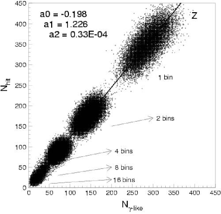
Figure 21: ${N_{\gamma-{\rm like}}}$ vs. ${N_{\rm ch}}$ correlation plot for various bins in $\phi$, obtained from normal events. Also shown are the correlation line and its parameters. From Ref. [143].

In this analysis method event-by-event correlation between ${N_{\gamma-{\rm like}}}$ and ${N_{\rm ch}}$ can be studied in different $\phi$-segments, by dividing the entire $\phi$-space into $2$, $4$, $8$ and $16$ bins of equal size. The correlation plot for each of the $\phi$-segments, starting with the case of one single bin – no segmentation – are shown in Fig. 21 for a sample of normal events. A common correlation axis ($Z$) is then obtained for the full distribution by fitting the ${N_{\gamma-{\rm like}}}$ and ${N_{\rm ch}}$ correlation with a second order polynomial. The correlation axis with fit parameters are shown in the figure. The distances of separation ($D_{Z}$) between the data points and the correlation axis is then calculated with the convention that $D_{Z}$ is positive for points below the $Z$-axis. The distribution of $D_{Z}$ represents the relative fluctuations of ${N_{\gamma-{\rm like}}}$ and ${N_{\rm ch}}$ from the correlation axis at any given $\phi$ bin.

Figure 22: $S_{Z}$ distribution for normal events (open circles) and DCC-type of events (solid histogram) with $\Delta\phi=90^{\circ}$ DCC domain. From Ref. [143].

One then applies this technique to simulated DCC events. The DCC events considered corresponds to a domain size of $90^{\circ}$ in $\phi$. In order to compare the fluctuations for different $\phi$ bins in the same level, one introduces a scaled variable, $S_{Z}=D_{Z}/s(D_{Z})$, where $s(D_{Z})$ represents the root-mean-squared (rms) deviation of the $D_{Z}$ distribution for normal events. The presence of events with localized fluctuations in ${N_{\gamma-{\rm like}}}$ and ${N_{\rm ch}}$ at a given $\phi$ bin is expected to result in a broader distribution of $S_{Z}$ compared to those for normal events at that particular bin. The typical $S_{Z}$ distributions for both class of events for 4 bins in $\phi$ are shown in Fig. 22. One clearly observes a difference in width of the $S_{Z}$ distribution between the two class of events. So the rms deviation of the $S_{Z}$ distribution quantifies the amount of fluctuation in such an analysis method.

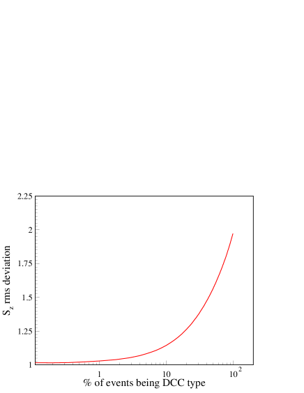
Figure 23: RMS deviation of $S_{Z}$ distribution for DCC-type of events with $90^{\circ}$ DCC domain in $\phi$ as a function of percentage of events being DCC-type. This plot shows the sensitivity of the method. From Ref. [143].

Figure 23 shows the sensitivity of the method for picking up DCC-type fluctuations for a case of $90^{\circ}$ domain size. The width of the $S_{Z}$ distribution has been plotted as a function of the number of events being DCC-type. As expected the rms deviation of $S_{Z}$ distribution increases with increase in $\%$ of DCC-type events in the sample.

This technique has been applied to WA98 experimental charged-particle and photon multiplicity data [18, 20, 21] to look for extra DCC-type fluctuations as compared to normal events.

3.3.2 Discrete wavelet analysis

The discrete wavelet technique (DWT), described in Sec. 2.4 above, has the beauty of analyzing a distribution of particles at different length scales with the ability of finally picking up the right scale at which there is a fluctuation. The method has been shown to be quite powerful to search for DCC-type of fluctuation [122, 124, 139]. Here we discuss how this method is actually appiled in analysing experimental data. As before, we analyze the simulated normal and DCC events using the multi-resolution DWT technique to search for bin-to-bin fluctuations in the charged-particle and photon multiplicity distributions. The analysis has been carried out in Ref. [139] by making $2^{j}$ bins in $\phi$ where $j$ is the resolution scale. The input to the DWT analysis is a sample distribution function at the highest resolution scale $j_{max}$. In most analysis presented below, the sample function corresponds to the photon fraction:

$$f_{\gamma}=\frac{{N_{\gamma}}}{{N_{\gamma}}+{N_{\rm ch}}}$$ (183)

where ${N_{\gamma}}$ and ${N_{\rm ch}}$ are the multiplicities of photons and charged particles respectively. The $\phi$-space is binned as discussed above and the analysis is carried out using the so-called $D-4$ wavelet basis [148]. The output of the DWT analysis consists of a set of wavelet or father function coefficients (FFCs) at each scale, from $j=0,\ldots,j_{max}-1$. The FFCs at a given scale carry information about the degree of fluctuation at higher scales. Due to the completeness and orthogonality of the DWT basis, there is no information loss at any scale. For the present study the analysis has been carried out by taking $j_{max}=5$.

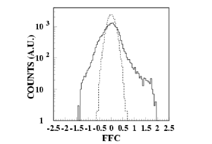
Figure 24: FFC distribution for simulated normal events and pure DCC-like events. The solid and the dotted lines correspond to the DCC-like and normal events respectively. From Ref. [147].

Typical FFC distributions at the scale $j=1$ are shown in Fig. 24. The dashed histogram represents the FFC distribution for normal events. The solid line histogram shows the corresponding distribution when a DCC domain of size given by $\Delta\phi=90^{\circ}$ and $3\leq\eta\leq 4$ is introduced in all the events. This constitutes an ensemble of DCC events having probability $\alpha=1$ of occurrence of a DCC. It is observed that the distributions for normal events is Gaussian, whereas there is a broadening of the distribution in the presence of DCC. The presence of a DCC domain modifies the phase space distributions of charged particles and photons, resulting in an increase in the rms deviations of the FFC distribution. So in this analysis the rms deviation, $s$, of the FFC distribution quantifies the amount of fluctuation.

To quantify the DCC-type effect further, we introduce a strength parameter $\zeta$, given by:

$$\zeta=\frac{\sqrt{(s_{\rm DCC}^{2}-s_{\rm normal}^{2})}}{s_{\rm normal}}\,,$$ (184)

where $s_{\rm normal}$ is the FFC rms deviation for an ensemble of normal events and $s_{\rm DCC}$ is the same for an ensemble of events with DCC. Figure 25 shows the sensitivity of the method for picking up DCC-type fluctuations for a case of $90^{\circ}$ domain size. The strength parameter derived from the rms deviation of the FFC distributions of normal and DCC type events has been plotted as a function of the fraction of events being DCC-type. As expected $\zeta$ increases with the latter.

This technique has been adopted by the WA98 Collaboration, which measures multiplicities of charged particles and photons in overlapping parts of the detector phase-space [20, 21].

Figure 25: Variation of $\zeta$ as a function of percentage of events being DCC type. DCC events have $90^{\circ}$ DCC domain in $\phi$. This plot shows the sensitivity of the method. From Ref. [143].

3.3.3 Robust observables

This analysis uses ratios of factorial moments of the charged-neutral pion distribution, as described at length in Sec. 2.4. It has been developed for a dedicated DCC search at the Fermilab TEVATRON by the MiniMAX Collaboration [17]. The set of robust observables is defined by Eqs. (142)-(143), where ${n_{\gamma}}$ and ${n_{\rm ch}}$ are given by the photon and charged-pion multiplicities respectively in the studied region of phase-space. For an inclusive analysis, the $n$’s denote the particle multiplicities in an event and averages are taken over a large number of events. For event-by-event analysis, when the multiplicity is high, the phase space region is divided into bins and the $n$’s denote the multiplicities in a bin. In this case, averages are taken over the total number of bins. As emphasized previously, the variables $r_{i,1}$ are robust observables in the sense that the detection efficiencies, often difficult to estimate – especially for photons, mostly cancel out and are thus expected to have little influence on the results. The main point [121] is that $r_{i,1}=1$ for all $i\geq 1$ in the case of generic pion production, whereas $r_{i,1}=1/(i+1)$ (see Eq. (147)) for pure ideal DCC production. Application of this technique to simulated normal and DCC-type events are shown in Fig. 26.

This technique has been used by the MiniMAX Collaboration [17] and also to analyze cosmic ray experimental data at Pamir.

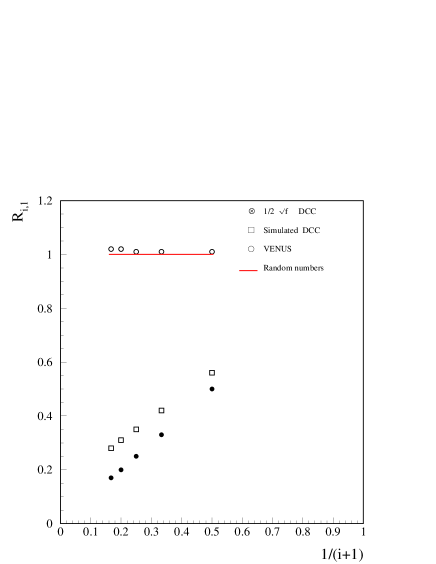
Figure 26: Results of inclusive DCC analysis using robust observables. Normal events (VENUS event generator) do not show any correlation whereas pure DCC events follow the relationship given in Eq. (147). The simulated DCC events generated by taking detector effects into account follow a similar behavior to that of pure DCC events. From Ref. [143].

3.3.4 $\Phi$-measure

The $\Phi$-measure for a system of particles is defined as [149, 150]:

$$\Phi=\sqrt{\langle Z^{2}\rangle\over\langle N\rangle}-\sqrt{\overline{z^{2}}}\,.$$ (185)

where $z=x-\overline{x}$, where $x$ is the value of a given single-particle observable in a given event and $\overline{x}$ its average over all particles and all events. The event variable $Z$ is a multi-particle analog of $z$ defined as $Z=\sum_{i=1}^{N}(x_{i}-\overline{x})$, where the summation runs over all particles from a given event. The brackets in (185) represent averaging over all events. Note that, by construction, $\overline{z}=0$ and $\langle Z\rangle=0$. As described in Refs. [151, 152], the $\Phi$-measure can be used to study the fluctuations in particle species. In that case, the single-particle variable $x=1$ if the particle is of a given sort (say a neutral pion) and $x=0$ otherwise (charged pion). This has been applied to study fluctuations of the neutral pion fraction $f$ from a DCC in Ref. [146].

Denoting by $N_{\pi}=N_{\pi^{0}}+N_{ch}$ the total pion multiplicity in a given event, one can write $N_{\pi^{0}}=fN_{\pi}$ and $N_{\pi^{\pm}}=(1-f)N_{\pi}$, where $f$ is the fraction of neutral pion in the event. Assuming that the relative fluctuations in $N_{\pi}$ are small, that is $\langle\delta N_{\pi}^{2}\rangle\ll\langle N_{\pi}\rangle^{2}$, one obtains [146]:

$$\Phi\simeq\sqrt{\langle N_{\pi}\rangle{\langle\delta f^{2}\rangle}}-\sqrt{\langle f\rangle\langle 1-f\rangle}\,.$$ (186)

It is instructive to consider the properties of the $\Phi$-measure in the following simple cases:

• Non-DCC case:
  It is known from $pp$ experiments [153] that the produced pions have their charge states partitioned binomially with $\langle f\rangle=1/3$. The fluctuation in $f$ is inversely proportional to the total number of pions and is approximately given by ${\langle\delta f^{2}\rangle}\approx\langle f\rangle\langle 1-f\rangle/\langle N_{\pi}\rangle$. In that case, one obtains, for the $\Phi$-measure:

  $$\Phi_{\rm non-DCC,~{}uncorr.}=0\,.$$ (187)

• No DCC, but $N_{\pi^{0}}$ and ${N_{\rm ch}}$ have non-trivial correlations:
  If $N_{\pi^{0}}$ and $N_{\pi^{\pm}}$ are assumed to be correlated in such a way that there are no (DCC-type) event-by-event fluctuations of the neutral fraction $f$. Moreover, the latter is assumed to be strictly independent of the event multiplicity. Then, $f=\delta$, where $\delta$ is a constant smaller than unity, and ${\langle\delta f^{2}\rangle}=0$. One has:

  $$\Phi_{\rm non-DCC,~{}corr.}=-\sqrt{\delta(1-\delta)}\,.$$ (188)

  Notice that The $\Phi$-measure is negative in that case.
  

• Ideal DCC case:
  For ideal DCC production, the probability distribution of the neutral fraction is given by the inverse square-root law, Eq. (10). One has $\langle f\rangle=1/3$ and $\langle\delta{f}^{2}\rangle=4/45$, so the $\Phi$-measure is given as:

  $$\Phi_{\rm DCC}=\sqrt{\frac{4\langle N_{\pi}\rangle}{45}}-\sqrt{\frac{2}{9}}\,.$$ (189)

  It is positive for $\langle N_{\pi}\rangle>5/2$. For a typical case where the total pion multiplicity $N_{\pi}\approx 300$, one finds $\Phi_{\rm DCC}\approx 4.7$. It is worth emphasizing that this assumes that all the observed pions are of DCC origin. A more realistic case would include pions from non-DCC sources as well [143]. This, along with the decay of neutral pions to photons as well as detector effects, have been discussed in Ref. [146].

Figure 27: Variation of $\Phi-\Phi_{\rm normal}$ as a function of the fraction $\beta$ of DCC pions, obtained from simulated data using VENUS. From Ref. [146].

The $\Phi$-measure can be applied to simulated data (both normal and DCC-type) in order to study the sensitivity of the measure to detection of DCC-type fluctuations. First we study the effect of varying the fraction $\beta$ of DCC pions in each event. To this aim, one calculates the quantity $\Phi-\Phi_{\rm normal}$, where $\Phi$ denotes the measure of fluctuation for a given DCC pion fraction $\beta$ and $\Phi_{\rm normal}$ is the measure of fluctuation for normal simulated events (detector and decay effects included). The variation of $\Phi-\Phi_{\rm normal}$ as a function of $\beta$ is shown in Fig. 27. One observes that the size of anomalous fluctuations decreases with decreasing DCC pion fraction, which is as per expectation. The statistical error on $\Phi$ was calculated to be $0.006$, from which one finds that such observable is a sensible probe of possible DCC-type fluctuations if the fraction of DCC pions in a typical event is above $\sim$ $3\%$.

Figure 28: Variation of $\Phi-\Phi_{normal}$ as a function of the DCC event fraction ($\alpha$) for a fixed DCC pion fraction ($\beta$ = 0.25), obtained from simulated data using VENUS. From Ref. [146].

This analysis assumes that all events have DCC pions. Including the effect of the probability of DCC formation being $\alpha\neq 1$ has been studied for a fixed fraction of DCC pions in each event in Ref. [141]. There, the authors assume that for DCC-type events the percentage of DCC pions is $\beta=0.25$ and vary the fraction $\alpha$ of events being DCC-type. The results are presented as $\Phi-\Phi_{\rm normal}$ vs. $\alpha$ in Fig. 28. As expected, the value of $\Phi-\Phi_{\rm normal}$ decreases with decreasing $\alpha$. Keeping in mind the above mentioned statistical error on $\Phi$-measure, we find that for $\beta=0.25$, the measure is sensitive to DCC formation if the latter occurs in more than $1\%$ of the events.

3.3.5 Event shape analysis

This method has been proposed in the context of DCC search in Ref. [147]. It is based on a technique that has been used successfully for flow analysis of heavy-ion data [154]. It uses the fact that localized DCC formation should lead to an event-shape anisotropy, which is expected to be out of phase for one detector (e.g. charged pions) compared to the other (e.g. photons). In other words, whenever there is large number of charged particles from a DCC region recorded in a given region of the first detector, there should be a depletion in the number of neutral particles recorded in the corresponding zone of the other detector. Therefore, from an event shape analysis using both detectors one can, in principle, look for DCC signals. In terms of the terminology used in flow analysis, this method is based on the fact that a simple redistribution of particles, with two detectors to detect charged particles and photons, would result in the same flow direction with the flow angle difference peaking at zero. However, events where the neutral pion fraction has been modified according to the ideal DCC probability distribution, will show the flow angles in two detectors to be almost $90^{\circ}$ apart [147].

In Ref. [147], events with localized DCC domains were simulated along the lines described earlier in Sec. 3.2 and event anisotropy (indicating flow) was introduced according to the following simple procedure. First, a flow direction is selected at random, uniformly distributed between $0^{\circ}$ and $360^{\circ}$. The directions of particles are then distributed about this direction following a Gaussian distribution with a width of $10^{\circ}$. Results were analyzed using the standard second order Fourier analysis of elliptic flow [154]. The particle hits in a given detectors can be labeled by their positions in the $\eta-\phi$ plane. For each event, one constructs the two sums:

$$X = \sum_{i}\cos(2\phi_{i})$$ (190)

$$Y = \sum_{i}\sin(2\phi_{i})\,,$$ (191)

where $\phi_{i}$ is the azimuthal angle of the particle $i$ and the sums run over all particles in a given event. The flow angle $\Xi$ is defined as:

$$\Xi={1\over 2}\arctan(Y/X)\,.$$ (192)

In the absence of any detector imperfections and other geometrical effects, the distribution of $\Xi$, taken over a large number of events, is expected to be completely flat over $0^{\circ}$ to $180^{\circ}$. This is because the flow direction varies randomly from event to event. However, when the events are realigned, with respect to the flow angle in each event, as described above, one can see the characteristic peaks (at $0^{\circ}$ and $180^{\circ}$) in the azimuthal distribution of particles.

In case of two detectors with the same phase space ($\eta-\phi$) coverage, one detecting photons and other detecting charged particles, the situation is very interesting. If there is genuine flow in a particular event both detectors would show the effect in terms of their respective $\Xi$-angles getting aligned in the same direction. Therefore the distribution of $\Psi=\Xi_{\gamma}-\Xi_{\rm ch}$, the difference between the flow angles of the two detectors, is expected to be peaking at zero. However, in case of DCC being prominent in a particular region, there will be more photons detected in one detector. The other detector is expected to show less charged particles in the same region of phase space. Therefore an event shape analysis is expected to show two flow angles for both detectors which will be out of phase (for the present second order Fourier analysis the angular difference is expected to peak at $90^{\circ}$).

The results of Ref. [147] are presented in Fig. 29. The three left panels (a)-(c) correspond to the case with only DCC in which one can notice (panel (a)) a clear peak at $90^{\circ}$ for the angle $\Psi$ between the event planes for the two detectors. Panels (b) and (c) show the angle between the event planes as obtained for two sub-events in each of the detectors separately. It is important to notice that both detectors show flow, but one with respect to the other clearly shows an anti-flow type behavior. In the same figure is also presented the data corresponding to pure VENUS events for comparison. One notices that the latter do not present neither any signature of flow nor DCC-like fluctuation. Finally, results shown in panels (d)-(f) show the same plots for flow type events which have no DCC-like fluctuation. Here, the individual detectors are seen to show the same effect as one with respect to the other.

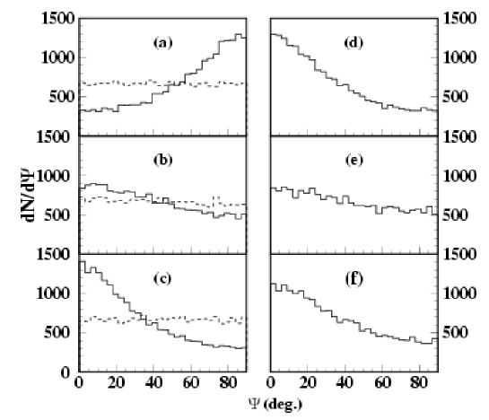
Figure 29: The distribution of $\Psi$ for simulated DCC (a)-(c) and flow (d)-(f) events. Panel (a) shows anti-correlation between event planes determined for charged-particle and photon detectors. Panels (b) and (c) show correlations between event planes obtained considering two sub-events for the photon and charged-particle detectors respectively. The dotted lines correspond to generic VENUS events. In case of flowy events, panels (d) shows correlation between event planes obtained from the two detectors, whereas panels (e) and (f) are analog to (b) and (c). From Ref. [147].

A more detailed analysis Ref. [147] reveals that this method is sensitive if at least $10\%$ of the events are of DCC-type. It has been argued that one can improve upon this by combining with the DWT technique Ref. [147] . The event-shape analysis has not yet been applied to experimental data.

3.4 Experimental results

We have discussed in the above section, the experimental set-up for various experiments looking for DCC and the experimental techniques used to look for DCC-type fluctuations in experimental data. Below we present the results from various experiments which have looked for possible DCC formation in high energy collisions.

3.4.1 Results from cosmic ray experiments

There have been many cosmic rays experiments [6, 7]. Here we discuss the most recent results from a systematic study of the large asymmetries in the neutral pion fraction distribution in high-energy cosmic-ray families (100 TeV $\leq$ $E_{visible}$ $\leq$ 700 TeV) detected at high mountain altitudes at Pamir [7]. The experimental data has been analyzed using the technique of robust observables discussed earlier. The results for the robust ratios $r_{i,1}$ is presented as a function of leading jet energy $E_{lead~{}jet}$ in Fig. 30. The pattern of energy flow in cosmic-ray interactions is understood through the picture of jets: The stream of energy in the air cascade are represented by jets produced in the nuclear interactions. In this picture the leading jet represents the pattern of atmospheric nuclear and electromagnetic cascade having the largest energy flow.

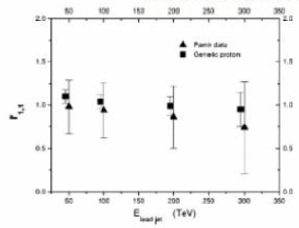
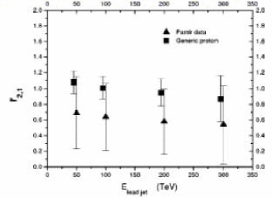
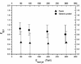
Figure 30: The robust observable $r_{1,1}$, $r_{2,1}$ and $r_{3,1}$ as a function of visible leading jet energy: experimental points are represented by triangles, whereas squares are used for simulated data. From Ref. [7].

From the figures one observes that the absolute values of $r_{i,1}$ are decreasing with increasing energy of the jets and the order $i$ of the moments. The results from data have been compared to simulated generic events. One observes that with the increasing order of the robust observables the difference between experiment and simulation becomes more important. Recall that values of $r_{i,1}$ far below 1 can be an indication of events with DCC formation overlaying generic events. The experimental average values of $r_{3,1}$ that are most sensitive to DCC formation are clearly below $1$ but by less than a standard deviation. The averaged experimental values for $r_{3,1}$ are presented in Table 2, together with the $95\%$ confidence interval. The latter does not exceed $1$.

Table 2: Experimental statistics and $95\%$ confidence interval of the average $r_{3,1}$ in Pamir experiment. From Ref. [7].

Jet energy (TeV)	$r_{3,1}$	Number of events	95% confidence interval
50	0.48 $\pm$ 0.44	78	(0.38,0.58)
100	0.45 $\pm$ 0.41	61	(0.38,0.55)
200	0.43 $\pm$ 0.40	30	(0.28,0.58)
300	0.47 $\pm$ 0.49	10	(0.12,0.82)

The conclusion from Pamir experiment [7] is that, due to the limited large error bars, the experimental data neither confirm nor rule out the possibility of a DCC formation mechanism in high-energy cosmic-ray interactions. A further increase in experimental statistics is needed to establish firm conclusions.

3.4.2 Results from nucleon-nucleon collision experiments

Here we discuss results on DCC search from high-energy nucleon-nucleon experiments UA1 and UA5 at CERN [13, 14, 15] and MiniMAX at Fermilab [17].

The UA5 Experiment

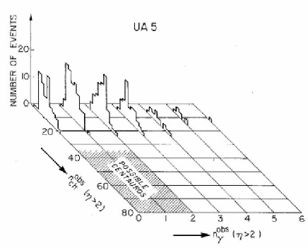
Figure 31: Number of events plotted against multiplicities of charged particles observed in the pseudo-rapidities interval $-2\leq\eta\leq 2$. The distributions are drawn separately for each value of observed photon multiplicity in the same range of pseudo-rapidity. The region which is populated by Centauro-like events if produced at the collider and observed by the detector is indicated. From Ref. [14].

Figure 31 shows the distribution of events as a function of observed charged-hadron multiplicity in the pseudo-rapidity interval $-2\leq\eta\leq 2$ for each value of observed photon multiplicity in the same interval, for $p\bar{p}$ collisions at center of mass energy of 540 GeV [14]. This correlation plot does not support the existence of Centauro type of events, based on the characteristics of Centauros observed in cosmic ray interactions. One observes that there is no event with charged hadron multiplicity remotely comparable to the expected value of $30-40$ with associated photon multiplicity being close to zero. The shaded portion represents the region where one would expect some events in $p\bar{p}$ collisions at $\sqrt{s}$ = 540 GeV, had they similar characteristics as Centauro events in cosmic-ray experiments.

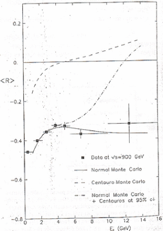
Figure 32: The asymmetry in electromagnetic and hadronic energy ($R$) is plotted along the Y-axis and the transverse energy is plotted along the X-axis. Comparison to various model calculations are shown. From Ref. [15]

The UA5 Collaboration [15] also looked for Centauro-like events in the $900$ GeV center of mass energy data, by studying the correlation of produced charged particles ${N_{\rm ch}}$ versus photons (${N_{\gamma}}$) and correlation between the electromagnetic ($E_{\rm em}$) and hadronic energies ($E_{\rm had}$) deposited in the calorimeters. Figure 32 shows the average value of the ratio

$$R=\frac{E_{\rm had}-E_{\rm em}}{E_{\rm had}+E_{\rm em}}$$ (193)

as a function of the transverse energy $E_{T}$, for experimental data, simulated normal and Centauro-like Monte-Carlo events, as well as a mixture of normal and Centauro events, the percentage of Centauro events being $0.24\%$ of all events. The data clearly seems to follow the trend of normal events. Further the correlation of ${N_{\rm ch}}$ with respect to ${N_{\gamma}}$ for data and Monte-Carlo simulation look similar, thereby ruling out the possibility of Centauro events or DCC-type events in the experimental data.

The UA1 Experiment

The UA1 Collaboration [13] have looked for Centauro-type events in $p\bar{p}$ collisions at center of mass energy of $540$ GeV in $48,000$ low bias events. They have measured the correlation between deposited transverse electromagnetic and hadronic energies, where the energy deposited in the first four radiation lengths of material is termed as electromagnetic energy and that deposited beyond twelve radiation lengths is termed as hadronic energy. By comparing experimental data with Monte-Carlo simulations, they have excluded possible Centauros or global DCC-type events in their data sample.

The MINIMAX Experiment

The analysis of the $p\bar{p}$ collisions data at center of mass energy of $1.8$ TeV for the MiniMAX experiment [17], in the forward direction $3.2\leq\eta\leq 4.2$, was carried out using the technique of robust observables, which, as already emphasized, had been actually developed for this experiment. A total of $1.3\times 10^{6}$ events was analyzed. A detailed Monte-Carlo simulation specific to the MiniMAX experiment, with input being minimum bias PYTHIA events passed through full detector simulation and analysis chain, yielded a value of $r_{1,1}\sim 1.02-1.13$ for the lowest robust ratio. A similar simulation with pure ideal DCC introduced by hand yielded a value of $r_{1,1}\sim 0.6-0.7$. This demonstrated the sensitivity of the experiment to detect a single large ideal DCC. The analysis of the data reveals that the ratios $r_{i,1}$ are not smaller than one as would be expected for pion production from a DCC. The measured values of the ratios $r_{i,1}$ are given in Table 3.

Table 3: Values of $r_{i,1}$ for the whole event sample (about $13.8\times 10^{5}$ events) of the MiniMAX experiment [17].

	$i$			$r_{i,1}$
	$1$			$1.026\pm 0.004$
	$2$			$1.035\pm 0.010$
	$3$			$1.059\pm 0.027$
	$4$			$1.118\pm 0.065$
	$5$			$1.310\pm 0.151$
	$6$			$1.904\pm 0.382$

The MiniMAX Collaboration was able to put some limits on DCC production in terms of the size of the DCC – that is the number of DCC pions produced – and the likelihood of DCC production. To this aim, two types of model for DCC production have been considered:

• Associated production, where the number of produced DCC pions in each event is proportional to the number of generically produced pions;

• Exclusive production, where a given event is described by either pure DCC or pure generic production with an given probability.

Knowing the most probable lower limit of the ratios $r_{i,1}$ in data, they were able to extract an upper limit on DCC production for the above two scenarios. For the associated production model, the upper limit on DCC pion production has been set at

$$\frac{\langle N\rangle_{\rm DCC}}{\langle N\rangle_{\rm generic}}\lesssim 0.21\,.$$ (194)

For the exclusive production model, the upper limit on DCC production is set in terms of probability that an event is DCC type. This value must be less than $0.05$.

3.4.3 Results from nucleus-nucleus collision experiments

Here we discuss results on DCC searches from the high-energy heavy-ion collision experiments at the CERN SPS (WA98 [20] and NA49 [19] Collaborations) and at the RHIC (PHENIX Collaboration [22]).

The WA98 Experiment

DCC search in WA98 experiment involved three kinds of analysis. One was to look for global DCCs [18], that is single large DCC domains, by measuring photon versus charged-particle correlation in the full common $\eta-\phi$ phase-space of the photon (PMD) and charged-particle (SPMD) detectors. Second was to look for smaller domains of DCC in common localized regions of $\eta-\phi$ phase space of the PMD and SPMD [20, 21]. And the third was to look for anti-Centauro–type events in the data by looking at localized regions in the event displays [155], as for example in the JACEE cosmic-ray experiment. Below we discuss the results on DCC search from the above three analysis carried out by the WA98 Collaboration.

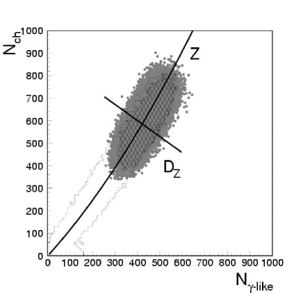
Figure 33: This is the scatter plot showing the correlation between ${N_{\rm ch}}$ and ${N_{\gamma-{\rm like}}}$. The solid outline shows the trend of the minimum bias data. The central sample (with $E_{T}>300$ GeV) is shown as points for the data and as a hatched region for VENUS (with much lower statistics). Overlaid on the plot are the $Z$ axis and the $D_{Z}$ axis at a particular value of $Z$ as explained in the text. From Ref. [18].

- Global DCC search:
The WA98 Experiment attempted to look for DCC-type fluctuations by looking at event-by-event correlation in the number of charged particles and photons detected over the full common $\eta-\phi$ coverage of the PMD and the SPMD [18]. The strong correlation between charged and neutral multiplicities shown in Fig. 33 suggests to employ a coordinate system with one axis being the measured correlation axis and the other being perpendicular to it. If all detected particles were pions and the detectors were perfect and had identical pseudo-rapidity acceptance, then the correlation axis would be a straight line. The details of the correlation analysis has already been described in Sec. 3.3.1. Here we present the results of such analysis applied to the WA98 data.

Figure 34: $S_{Z}$ distribution for the experimental data is shown, overlaid with VENUS simulations incorporating $0\%$, $25\%$ and $60\%$ DCC-type events. All of the distributions are normalized to the total number of data events. From Ref. [18].

The $S_{Z}$ distribution for both data and simulated events are shown in Fig. 34. The simulated events have been generated using the VENUS 4.12 event generator, with output processed through a detector simulation package in the GEANT 3.21 framework [156]. This incorporates the full WA98 experimental setup. The centrality selection for simulated data has been made in an identical manner as in the data, determined from the simulated total transverse energy of mid-rapidity calorimeter used in the experiment. The discrepancy between VENUS and the data can be seen more clearly by measuring the width of the $S_{Z}$ distribution. The simulated and measured distributions are both Gaussian with respective widths $\sigma_{\rm simul.}=0.998\pm 0.002$ (fit error only) and $\sigma_{\rm meas.}=1.13\pm 0.07$ (error from relative scale uncertainties included).

Figure 35: The $90\%$ C.L. upper limit on DCC production per central event as a function of the fraction of DCC pions under two assumptions. The thick line gives the upper limit obtained by assuming the $\sigma_{D_{Z}}$ in $S_{Z}$ is completely given by the VENUS calculation requiring to make a cut at $6\sigma$. The dashed line shows a less conservative limit obtained by using the $\sigma_{D_{Z}}$ measured in the data itself. This allows one to make a tighter cut at $5\sigma$, increasing the DCC detection efficiency. From Ref. [18].

One expects that DCC events would show up as non-statistical tails on the $S_{Z}$ axis. No such events were seen by the WA98 Collaboration in their global analysis of the data sample. They concluded that a possible single DCC domain is either very rare, very small, or both. To check which hypothese is consistent with their data, they determined upper limits on the frequency of DCC production as a function of its size, as represented by the fraction $\beta\equiv\zeta=N_{\rm DCC}/N_{\pi}$ of DCC pions. For this they have computed $S_{Z}$ distributions for several values of $\zeta$, ranging from $15\%$ to $90\%$, and they have considered two possible scenarios. The first is based upon the conservative assumption that VENUS should describe the data perfectly in the absence of a DCC signal. The corresponding $90\%$ C.L. excluded region for possible DCC formation is presented in Fig. 35 as a solid line. The second scenario assumes that the difference between the data and VENUS seen in Fig. 34 is due to detector effects and that the widths should in fact be the same. The resulting excluded region is shown in Fig. 34 as a dashed line. The boarders of the two regions are quite different at $\zeta=15\%$, but get closer at $\zeta>30\%$.

- Search for localized domains of DCC:
Photon and charged-particle multiplicity correlation studies have also been carried out in localized regions of the $\eta-\phi$ phase-space to look for the possible existence of small localized DCC domains. This analysis uses both the techniques of ${N_{\gamma}}-{N_{\rm ch}}$ correlation and DWT in various bins in azimuthal angle [20, 21], discussed previously under sections 3.3.1 and 3.3.2. The WA98 Collaboration have also studied the centrality dependence of this analysis. For this, four different centrality bins were considered: top $5\%$ (henceforth referred to as centrality-1); $5\%-10\%$ (centrality-2); $15\%-30\%$ (centrality-3); and $45\%-55\%$ (centrality-4) of the minimum bias cross-section.

In looking for non-statistical DCC-type fluctuations in experimental data, it is necessary to understand all detector related effects and to try to filter out the various components contributing to the total observed fluctuations. For this, results from experimental data need to be compared to some base line results to draw proper conclusions. Due to the inherent uncertainties in the description of “normal” physics and detector response in simulations, the observation of an experimental result which differs from the case with statistical fluctuation, given by simulations, cannot be taken alone as evidence of presence of non-statistical fluctuations. This problem can be solved by generating different sets of mixed events from data, keeping specific physics goals and detector effects in mind. This remarkable ability of mixed events to probe different physics goals is possible through construction of suitable ensembles of mixed events by removing various correlations in a controlled manner while preserving the characteristics of the measured distributions as accurately as possible. Fluctuations in the ratio of ${N_{\gamma}}$ to ${N_{\rm ch}}$ can have three different origins: They can arise due to independent fluctuation in either ${N_{\gamma}}$ only, ${N_{\rm ch}}$ only, or both. Further, in the latter case the fluctuations in ${N_{\gamma}}$ and ${N_{\rm ch}}$ may be correlated event by event. In particular, such a correlation is expected to arise in the case of DCC production. By intelligently constructing different types of mixed events one can probe possible non-trivial fluctuations in the ${N_{\gamma}}$-to${N_{\rm ch}}$ ratio and their origin.

A first set of mixed events, referred to as M1-type, is constructed to provide a base line for comparison to real event. These are generated by mixing hits in both photon (PMD) and charged-particle (SPMD) detectors separately, satisfying the ${N_{\gamma-{\rm like}}}-{N_{\rm ch}}$ correlation as in the real event. This is done by producing one mixed event for each real event with the same multiplicity of ${N_{\gamma-{\rm like}}}$ and ${N_{\rm ch}}$ pair as in the VENUS event. The idea is to globally keep the distributions similar to real events and look for event-by-event fluctuations in localized regions of phase-space. In the construction of such mixed events, care is taken such that no two hits come from the same real event. Moreover, hits within a detector in the mixed events are not allowed to lie within the two track resolution of the detector. Results from such mixed events when compared to those of real events were expected to reveal the presence of localized fluctuations. However, they do not give any information neither regarding the origin of such fluctuations nor concerning possible ${N_{\gamma}}-{N_{\rm ch}}$ correlations.

A second set of mixed events, referred to as M2-type events, has been constructed to provide information regarding the possible presence of localized event-by-event correlated fluctuation in ${N_{\gamma-{\rm like}}}$ and ${N_{\rm ch}}$. They are generated by mixing photon events with different charged-particle events so that no two events were repeated. Here also, care is taken that the original ${N_{\gamma-{\rm like}}}-{N_{\rm ch}}$ correlation is maintained. The original event-by-event hit structure in each individual detector being left unchanged, such mixed event set keeps identical the individual localized fluctuations due to ${N_{\gamma-{\rm like}}}$ and ${N_{\rm ch}}$, but removes possible event-by-event correlations. Therefore, by comparing the results from such mixed events to those from real events reveals the presence of localized event-by-event correlated fluctuations in ${N_{\gamma-{\rm like}}}$ and ${N_{\rm ch}}$.

Finally, two other sets of mixed events, referred to as M3-$\gamma$ and M3-ch type, have also been considered to provide information regarding contribution to localized fluctuations in the ${N_{\gamma}}$-to-${N_{\rm ch}}$ ratio from either ${N_{\gamma}}$ fluctuations or ${N_{\rm ch}}$ fluctuations separately. Such events are generated from real events by mixing hits in one of the detectors (following the procedure of construction of M1-type events) and keeping the hit structure of the event in the other detector intact. M3-$\gamma$ events corresponds to the case where the hits within the photon detector are unaltered while the charged-particle hits from different events are mixed, whereas M3-ch events correspond to the opposite case. The total number of mixed events generated is the same as the number of real events. Results from such mixed events, when compared to those of real and M1-type events, are expected to reveal the presence of event-by-event localized fluctuations in ${N_{\gamma-{\rm like}}}$ and ${N_{\rm ch}}$ individually. The various sources of fluctuation in the ${N_{\gamma}}$-to-${N_{\rm ch}}$ ratio which are preserved by the different types of mixed events described above are summarized in Table 4.

Table 4: Sources of fluctuations preserved by various mixed events.

Type of			Mixed	Event
fluctuation		M1	M2	M3-$\gamma$	M3-ch
${N_{\gamma}}$ only		No	Yes	No	Yes
${N_{\rm ch}}$ only		No	Yes	Yes	No
correlated ${N_{\gamma}}-{N_{\rm ch}}$		No	No	No	No

Mixed events constructed from experimental data were compared to simulated events, generated as for the global DCC case discussed previously, and were analyzed using both the correlation and the DWT analysis techniques. Since the widths (rms deviations) of the $S_{Z}$ and FFC distributions carry the information concerning fluctuations, below we compare these widths as obtained from data as well as mixed and simulated events.

\begin{picture}(100.0,100.0)(10.0,10.0)\put(0.0,60.0){ \epsfbox{figures/expt_23.eps} } \put(60.0,60.0){ \epsfbox{figures/expt_24.eps} } \put(0.0,10.0){ \epsfbox{figures/expt_25.eps} } \put(60.0,10.0){ \epsfbox{figures/expt_26.eps} } \end{picture}

Figure 36: RMS deviations of the $S_{Z}$ distributions for data, mixed and simulated events for the four centrality bins: top-left for centrality-1, top-right for centrality-2, bottom-left for centrality-3 and bottom-right for centrality-4. From Ref. [21].

The rms deviations of the $S_{Z}$ distributions calculated at different $\phi$ bins are shown in Fig. 36 for data, mixed (M1, M2, M3-$\gamma$ and M3-ch) and VENUS events, in various centrality bins. The statistical errors on the values are small and are within the sizes of the symbol. The bars represent statistical and systematic errors added in quadrature. The total error is not more than $3\%$ for the most central events and goes to not more than $10\%$ for the most peripheral events. From Fig. 36, one observes that the nature of the rms deviations of the mixed events closely follow those of the data. The mixed events have been constructed such that the ${N_{\gamma-{\rm like}}}$ vs. ${N_{\rm ch}}$ correlations are maintained for full azimuth – that is one single bin, so the rms deviations of data and mixed events are identical by construction in that case. The rms deviations of M2-type events are found to agree with those of the experimental data within errors for all four centrality classes, thereby suggesting the absence of localized correlations in ${N_{\gamma-{\rm like}}}$ and ${N_{\rm ch}}$. The same for M1-type events are found to be lower than those obtained for data for $2$, $4$ and $8$ bins in $\phi$ for centrality bins $1$, $2$ and $3$. The results form M3-type events are found in between those obtained from data and M1-type events. These results indicate the presence of localized fluctuations in data, due to both photons and charged particles. However for the case of centrality-4, the rms deviations of $S_{Z}$ distributions from data and the mixed events are found to more or less agree with each other within the quoted errors. The rms deviations for the simulated events are $1$ for all bins in azimuth by definition of $S_{Z}$.

\begin{picture}(100.0,100.0)(10.0,10.0)\put(0.0,60.0){ \epsfbox{figures/expt_27.eps} } \put(60.0,60.0){ \epsfbox{figures/expt_28.eps} } \put(0.0,10.0){ \epsfbox{figures/expt_29.eps} } \put(60.0,10.0){ \epsfbox{figures/expt_30.eps} } \end{picture}

Figure 37: RMS deviations of the FFC distributions for data, mixed and simulated events for the four centrality bins: top-left for centrality-1, top-right for centrality-2, bottom-left for centrality-3 and bottom-right for centrality-4. From Ref. [21].

The rms deviations of the FFC distributions calculated at different $\phi$ bins are shown in Fig. 37 for data, all four types of mixed events, as well as generic VENUS events. We observe that the rms deviations of data, VENUS and mixed events match with each other (within quoted errors) for $32$ bins in $\phi$ for all the the four centrality classes. The VENUS results are close to the M1-type events, for centrality classes 1, 2 and 3 and are slightly higher for centrality-4. The rms deviations of the FFC distributions for M2-type events are found to agree closely with those for data for all centrality classes and all bins in $\phi$. The rms deviations for M3-type events lie in between those obtained from data and M1-type mixed events. These results are consistent with those obtained from the $S_{Z}$ distributions. They indicate the presence of individual localized fluctuations in photons and charged particles for certain bins in azimuth (resulting in fluctuations of the ratio, as seen). However, they show no clear evidence for localized correlated fluctuations (DCC-type) between ${N_{\gamma-{\rm like}}}$ and ${N_{\rm ch}}$.

Comparing these results with those obtained from simulated DCC events described in Sec. 3.2, one can extract an upper limit on the occurrence probability of DCC-like fluctuations at the $90\%$ confidence level, following the standard procedure [157] as described below. This has been done, in particular, for central Pb-Pb events with $E_{T}\geq 341$ GeV at $158$ AGeV collision energy, as DCC formation is expected to be more likely in these events. First, a quantity $\chi$ is defined as:

$$\chi=\frac{\sqrt{(s_{1}^{2}-s^{2})}}{s}\,,$$ (195)

where $s$ and $s_{1}$ correspond to the rms deviations of the FFC (or $S_{Z}$) distributions of M2-type mixed events and real data respectively. It is assumed that errors are Gaussian-distributed. Since errors are asymmetric one considers the largest error for the calculation to be on the conservative side. The errors on the rms deviations are propagated to get errors on $\chi$. Upper limit contours with $90\%$ C.L. have been calculated by taking the limit at $\chi+1.28e_{\chi}$ where $e_{\chi}$ is the error in $\chi$ from $S_{Z}$ and FFC analysis. The two upper limit contours set by the two different analysis were found to be consistent with each other. It must be mentioned that, for calculating the upper limits, it has been assumed that the total difference in rms values of data and M2-type events is due to DCC-like fluctuations. Now, to relate them to DCC domain size and frequency of occurrence of DCC, one proceeds as follows: Obtain the rms deviations of FFC distributions for various domain sizes (from $15^{\circ}$ to $180^{\circ}$ in $\phi$ with $15^{\circ}$ increments) for different values of the frequency of occurrence of DCC (varying from $0\%$ to $100\%$), where simulated DCC events are generated from the simple model discussed earlier. Then carry out the entire analysis as done for data to get $\chi$ values for each set of events. One then finds for which frequency of occurrence for a fixed DCC domain size, the $\chi$ value from simulation matches with that of the $\chi+1.28e_{\chi}$ for data. This is done for each of the above domain sizes. This is then used to set the upper limits in terms of domain size and frequency of occurrence of DCC, as shown on Fig. 38. It may be mentioned that results from both the $S_{Z}$ and FFC analysis methods gives similar upper limits.

Figure 38: $90\%$ confidence level upper limit on DCC production per central event at SPS as a function of DCC domain size in azimuthal angle within the acceptance of the detectors. The solid line is for top $5\%$ central events and dashed line for $5\%-10\%$ centrality class. From Ref. [21].

Thus, within the context of this simple DCC model, an upper limit on the presence of localized non-statistical DCC-like fluctuations is found to be of the order of $10^{-2}$ for an azimuthal domain size $45^{\circ}\lesssim\Delta\phi\lesssim 90^{\circ}$ and about $3\times 10^{-3}$ for $90^{\circ}\lesssim\Delta\phi\lesssim 135^{\circ}$. This upper limit is the most strict limit set so far at SPS. Compared to earlier limits set in global analysis of WA98 and NA49, this analysis is more sensitive to possible presence of small localized domains of DCC in $\eta-\phi$ phase-space.

-Search for anti-Centauro events: Finally, a new method to look for anti-Centauro events in WA98 data has been proposed [155], where one studies events having photon excess in azimuthal patches within the overlap zone of the PMD and the SPMD. One of the advantage of searching for anti-Centauro type events is that the purity of the photon sample observed by the PMD will be higher than those for normal patches due to the depleted flux of charged particles. The WA98 Collaboration have analyzed 196K events corresponding to the top $15\%$ of the minimum bias cross-section. One looks for fluctuations in the neutral pion fraction in localized regions of the $\eta-\phi$ phase-space on an event-by-event basis. A particular azimuthal window $\Delta\phi$ is selected in the pseudo-rapidity range $2.9<\eta\leq 3.75$ and the entire azimuthal range from $0^{\circ}$ to $360^{\circ}$ is scanned in order to find the patch having the maximum value of $f$, referred to as $f_{max}$. This scan is performed by successive $2^{\circ}$ rotations of the $\Delta\eta-\Delta\phi$ patch in the $\eta-\phi$ plane. To minimize the statistical fluctuations, a patch with maximum $f$ value in an event was required to have at least $40$ photons corresponding to a $15\%$ statistical error.

Figure 39: Plot showing photon hits (PMD) and charged particle hits (SPMD) in an azimuthal plane. The marked $90^{\circ}$ patch corresponds to $f_{max}$ = 0.77. From Ref. [155].

Results from such an analysis have been compared with simulated events obtained using the VENUS 4.12 event generator and processed through the WA98 detector setup using GEANT 3.21. These are referred to as V+G events. The statistical significance of these results is obtained by comparing them with those obtained from a similar analysis applied to the various types of mixed events discussed above. An event displaying PMD hits (filled circles) and SPMD hits (open squares) within the overlap $\eta-\phi$ zone (obtained by using the method described above) is shown in Fig. 39. The patch of size $\Delta\phi=90^{\circ}$ in azimuth having the highest neutral ratio $f$ is also marked. The number of charged particles in this patch is only $12$ as compared to $84$ photons, which corresponds to $f_{max}=0.77$. Figure 40 shows histograms of the maximum value $f_{max}$ of the neutral fraction in each event, for data, mixed events, and V+G events. This corresponds to a patch size of $\Delta\phi=60^{\circ}$. It is seen that the $f_{max}$ distribution for the data extends to much larger values than for mixed and V+G events.

Figure 40: $f_{max}$ distributions for 60^∘ patch for data (solid histogram), mixed Events (dashed histogram) and V+G (dotted histogram). From Ref. [155].

To test the authenticity of these events, the neutral pion fraction $f$ has also been calculated for the immediate preceding and succeeding events in the data in the same patch in $\eta-\phi$. The distribution of these $f$ values is shown in Fig. 41. The solid line corresponds to the neutral pion fraction for patches having $f_{max}>0.55$ with ${N_{\gamma}}>40$ and the dashed histogram represents the $f$ distribution for preceding and succeeding events in the data sample. The latter has its peak at about $0.35$, which is characteristic of generic (normal) events. This shows that events with $f_{max}>0.55$ are indeed special events, having large non-statistical charged-to-neutral fluctuations. In this sense , these events [155] may resemble the anti-Centauro events found in cosmic ray experiments [6].

Figure 41: Neutral pion fraction ($f$) distributions for events having $f_{max}>0.55$ (solid line) and for preceding and succeeding events (dashed line) for $60^{\circ}$ patch having ${N_{\gamma}}>40$. From Ref. [155].

In summary, using this new event-by-event analysis the WA98 have found events with large charged-to-neutral fluctuations in their data, which exhibit $f_{max}>0.55$ in certain $\Delta\phi$ domains. These domains are uniformly distributed in azimuth. The fraction of such events are much larger in the data as compared to those seen in the mixed events and V+G events. The percentage of these events increases significantly with decreasing patch size. Also the fraction of such events increases significantly as one decreases the centrality. The special events selected by this procedure appear anti-Centauro like [155] similar to those found in cosmic ray experiments [6]. A more careful analysis of the statistical significance of these events is needed to conclude about observation of DCC.

The NA49 Experiment

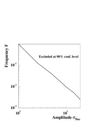
Figure 42: Limit on the amplitude of fluctuations in the $p_{T}$ parent distribution as a function of the frequency of occurrence of the event showing the fluctuation. From Ref. [19].

The NA49 Experiment, which detects only charged hadrons, has tried to put an upper limit on DCC production at SPS from the measurement of fluctuations in mean transverse momentum $M(p_{T})$ [19]. They argue that fluctuations in $M(p_{T})$ are also relevant for models of processes that lead to non-statistical fluctuations localized in transverse momentum, like the formation of DCCs. As we have seen previously in the theory review, pions emitted from DCC domains are expected to be preferentially produced at low transverse momenta. This provides a translation of the number-fluctuations, expected from dynamical DCC simulations (see Sec. 2.4), into $p_{T}$ fluctuations accessible to the NA49 experiment. For comparison purposes NA49 used the same type of simulated DCC events as the WA98 Collaboration [18], which we described in detail above. The DCC production is characterized by the probability $\alpha\equiv F$ to form a single DCC domain in an event and the fraction $\beta\equiv\xi$ of pions coming from the DCC. They made the additional assumption that the DCC pions are produced with $p_{T}<p_{T}^{max}=m_{\pi}$. The ratio of neutral to charged pions was chosen randomly according to the ideal DCC probability distribution of the neutral pion fraction, Eq. (10). The isospin fluctuations of pion production from DCCs then lead to multiplicity fluctuations of charged pions at low transverse momenta and, therefore, to non-statistical fluctuations in $M(p_{T})$. For DCCs occurring in every event ($F=1$) the fluctuations observed in the data rule out DCC sizes of $\xi>0.35$. The limit on the amplitude of fluctuations in the $p_{T}$ parent distribution as a function of the frequency of occurrence of the events showing the fluctuation is shown in Fig. 42.

RHIC experiments

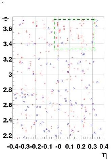
Figure 43: Centauro-type event seen in the PHENIX Experiment at RHIC. The solid circles are photon hits and plus signs are charged-particle hits. The box shows the Centauro region in $\eta-\phi$ phase-space. From Ref. [22].

Among the four RHIC experiments, both STAR [23] and PHENIX [158] have the capability to look for DCC-type fluctuations. So far the PHENIX Collaboration have reported [22] some results on search for Centauro and anti-Centauro type of events at RHIC energies. They use the photon information from the electromagnetic calorimeter and charged-track information using drift chamber and pad chamber detectors. One such typical possible Centauro event is shown in Fig. 43. The analysis is still in preliminary stage. In addition to looking for such events, they also carry out a multi-resolution analysis, with input being the asymmetry between the number of charged tracks and neutral clusters, on an event-by-event basis as a function of subdivided $\eta-\phi$ phase-space.

3.5 Possibility and limitations of DCC search

For detecting a DCC signal with very low probability of occurrence, it is necessary to understand, from an experimental point of view, all the factors that affect the detection of DCC domain during its transition from the time of formation to the time of detection. This has been investigated in Ref. [141] using the simple model for simulating DCC events described earlier. The analysis is carried out using the method based on the DWT technique and looking at the signal-to-background ratio. Possible factors that can affect the DCC signal are: effect of the $\pi^{0}$ decay; the presence of multiple DCC domains; detector related effects, such as efficiency and purity of particle detection; use (or lack) of $p_{T}$-information of the detected particles; increase in particle multiplicity as one goes from SPS to RHIC and LHC energies.

3.5.1 Effect of decay of $\pi^{0}$

Figure 44: Typical $f$ distributions inside a DCC domain before (solid line) and after decay (dotted line) of $\pi^{0}$ ($f^{\prime\prime}$). Also shown for comparison is the $f$ distribution for normal events (dashed line). From Ref. [141].

The formation of DCC leads to large event-by-event fluctuation in the neutral pion fraction $f$. To observe this in an ideal situation one has to count the number of neutral pions $\pi^{0}$ event-by-event. But the $\pi^{0}$’s decay into photons by the time they reach the detector. As a result, photons coming from DCC $\pi^{0}$’s inside a given DCC domain may move out of the $\eta-\phi$ phase-space of the domain – depending on their momentum – before they are detected. Also, photons from outside the DCC domain may enter the $\eta-\phi$ phase-space of the domain. Both effects result in dilution of the strength of the signal. Considering the effect of $\pi^{0}$ decay, one modifies Eq. (182) as:

$$f^{\prime\prime}=\frac{{N_{\gamma}}/2\pm\delta_{\gamma}}{{N_{\gamma}}/2\pm\delta_{\gamma}+{N_{\rm ch}}}\,,$$ (196)

where $\delta_{\gamma}$ is the resultant number of photons that get removed from or added into the DCC domain and ${N_{\rm ch}}$ is the number of charged pions in the region of $\eta-\phi$ phase-space under consideration. For multiplicity detectors (e.g. SPMD in WA98, or FMD in ALICE), which do not have the capability of particle identification, ${N_{\rm ch}}$ denotes the multiplicity of all charged particles in the considered phase-space region. Since $\delta_{\gamma}$ is a non-zero number, the possibility of observing a pure Centauro-type event ($f\ll 1$) is low. In fact the distribution of the ratio $f^{\prime\prime}$ will be shifted away from zero, as illustrated in Fig. 44, which shows the probability distributions for $f$ and $f^{\prime\prime}$ inside a DCC domain in the model calculation. Here ${N_{\rm ch}}\equiv N_{\pi^{\pm}}$. The effect of detecting other charged particles along with pions will be discussed later. Clearly one can notice that, as a result of $\pi^{0}$ decay, the peak of the original DCC distribution is shifted to a non-zero value $\simeq 0.15$. Also shown in the figure is the $f$ distribution for normal events. In that case, the $f$ and $f^{\prime\prime}$ distributions are not very different because the relative population of $\pi^{0}$ is the same within and outside the domain and hence the loss due to decay is compensated by the gain due to decay from other phase-space regions.

In order to quantify the decrease in the detectability of the DCC signal, the authors of [141] considered the following two cases:

• Analysis using a $\pi^{0}$ detector:
  In the first case one puts two hypothetical detectors, one for detecting $\pi^{0}$’s and other for detecting charged pions, with $100\%$ efficiency, within one unit of $\eta$ and full $\phi$ coverage. The detector effects will be discussed later taking realistic efficiency and other parameters. The goal here is to study the $\pi^{0}$ decay effect only. Then one introduces DCC domains in the simulated events with domain size $\Delta\phi$ varying from $30^{\circ}$ to $180^{\circ}$. These events without $\pi^{0}$ decay and having DCC domain of a particular size are then analyzed using the DWT method to obtain the FFC distribution. The strength parameter $\zeta$ is calculated from Eq. (184).

• Analysis using an ideal photon detector:
  In the second case one replaces the $\pi^{0}$ detector with an ideal photon detector having $100\%$ detection efficiency and no contamination from charged particles. The $\pi^{0}$’s are allowed to decay and a similar analysis as mentioned above is carried out to obtain the strength values.

From the two such obtained strength values for each DCC domain size, one calculates the percentage decrease in strength value of the second case (ii) compared to the first case (i). This is shown in Fig. 45 for various domain sizes in $\Delta\phi$. The results show that the decrease in strength of the signal is more for smaller domains of DCC as compared to larger ones. We mention that for each DCC domain size, two cases have been studied: one in which all the events have DCC-type fluctuations and another where only $20\%$ of the events have DCC-type fluctuations introduced. It is found that the results are similar for both cases.

Figure 45: Percentage decrease in the strength of DCC signal due to the effect of decay of $\pi^{0}$ as a function of domain size $\Delta\phi$. From Ref. [141].

3.5.2 Multiple domains of DCC

In heavy-ion collisions there is a possibility that more than one domain of DCC be formed, each with a chiral condensate pointing in independent directions in isospin space. Of course, the contribution to the neutral fraction from different independent domains is expected to reduce the DCC signal in isospin fluctuations [159]. In particular, in case of a large number of independent domains of equivalent size, one expects the distribution of the total neutral fraction $f$ to approach a Gaussian centered at $\langle f\rangle=1/3$ and of width inversely proportional to the square root of the number of domains, as per the central limit theorem. This makes the dis-entanglement of DCC signal from that of normal events difficult.

These effects have been studied in [141] using the multi-resolution DWT method. For simplicity, and in view of limitations of the model in terms of introducing DCC at the freeze-out stage, these authors have placed varying number of DCC domains in each event, depending on the domain size in $\Delta\phi$. All the domains are assumed to extend over one unit in pseudo-rapidity. For example, we can place up to four domains of $\Delta\phi=90^{\circ}$, without any overlap among themselves. These authors have also carried out the analysis by placing up to six DCC domains with $\Delta\phi=30^{\circ}$ in each event. Care has been taken in placing the domains randomly so that no two domains overlap. The $f$ value of each domain in each event is randomly chosen following the $1/2\sqrt{f}$ probability distribution. The aim is to see how the signal changes in terms of the strength parameter as given in Eq. (184).

Figure 46 shows the variation of strength of the DCC signal with the number of domains in a given event for two domain sizes of $\Delta\phi=90^{\circ}$ and $30^{\circ}$. One observes that the strength of the DCC signal increases as the number of domains increases and saturates for larger number of domains. The increase in strength value with increase in number of domains is because the multi-resolution event-by-event analysis based on the DWT method has been able to pick up signals by looking at bin to bin (in $\phi$) fluctuations in each event. It is worth emphasizing that this result is not in contradiction with the theoretical considerations described above [159, 160]. Indeed, if the multiple DCC domains formed in the initial stages, in the course of their evolution, move towards the same part of phase space covered by a detector, then the strength of the signal will reduce. However, if the phase space separation is maintained in evolving DCC domains, then the strength will increase as found in the present analysis.

Figure 46: Variation of the strength of DCC signal with increase in number of DCC domains in an event. All the events are DCC events. From Ref. [141].

3.5.3 Detector effects

The detector limitations are basically those related to efficiency and purity of particle detection and to the acceptance in $\eta-\phi$. The effect of efficiency of particle detection is trivial, higher the efficiency of particle detection, more reliable is the search for DCC. Similarly the role of higher acceptance in $\eta$ and full azimuthal coverage can be hardly over-emphasized (lower acceptance effectively reduces the total multiplicity of observable DCC pions and hence reduces the strength of the DCC signal). If the acceptance in $\eta$ is sizable, one can attempt DWT analysis using bins in $\eta$ for limited azimuthal coverage, which would be complementary to the various analysis reviewed here. Such an analysis would certainly be of great interest.

The purity of the photon sample, as measured in a detector like PMD, is around $60\%-70\%$, whereas that of charged particle samples measured using detectors like FTPC or FMD is quite high, larger than $95\%$. Hence we discuss here only the effect of purity of photon sample.

Effect of neutral pion fraction on the purity of photon sample

Figure 47: Variation of purity of the photon sample as a function of neutral pion fraction. For $f=0.33$ (generic event) purity is $\sim 0.74$. From Ref. [141].

It is of interest to study the effect of the DCC neutral pion fraction on the purity of the photon sample. Consider the case where the neutral pion fraction for a DCC domain is $f=1$. This corresponds to a situation where there are no charged pions. This will lead to greatly reduced number of charged particles falling on the photon detector. So the purity of the photon sample will be high. The variation of purity with neutral pion fraction can be investigated in the following manner [141]: The number of $\gamma$-like hits on the photon detector can be written as

$${N_{\gamma-{\rm like}}}=\epsilon{N_{\gamma}}+c{N_{\rm ch}}\,,$$ (197)

where the first term denotes the contribution of actual photons and the second term denotes charged-particle contamination. The factor $c$ is the fraction of charged-particles on the PMD acceptance treated as contamination to the detected photon sample. One assumes that the latter is given by a normal distribution with mean of $15\%$ and width of $5\%$, the percentage being taken with respect to the total charged particles within the acceptance of the photon detector. This is a reasonable number, considering that the converter thickness of the preshower detector is $\sim$ $10\%$ of an interaction length and some interactions lead to multiple clusters (the effect of overlapping clusters is ignored). DCC-type fluctuations are introduced for fixed $f$ values and domain size $\Delta\phi=360^{\circ}$ and $\Delta\eta=1$ in a set of event. Several such sets of events were generated for $f$ values varying from $0.025$ to $1.0$. The purity of the photon sample is then calculated for each set of events with a fixed neutral pion fraction value.

The results are shown in Fig. 47, where one clearly sees that the purity of photon sample increases with the increase in the neutral pion fraction value. However the purity does not reach a value of $1$ for $f$ = $1$, because there are charged particle other than $\pi^{\pm}$ falling on the detector. Similarly it never reaches a value of zero for $f$ = 0, as there are $\gamma$’s from $\pi^{0}$’s decaying outside the detector acceptance and from other sources.

Effect of charged-particle contamination in PMD

Figure 48: Variation of rms deviation of FFC distribution for pure VENUS events with increase in the percentage of contamination in the photon detector. The variation of rms deviation of FFC distributions of mixed events constructed form VENUS are also shown. From Ref. [141].

Photon measurement in heavy-ion collisions has the problem of charged-particle contamination. The charged particles detected as photons have a correlation with those detected in the charged-particle multiplicity detector. This additional correlation suppresses the possible anti-correlation between photons and charged particles that may arise due to DCC formation.

The effect of such a correlation has been studied in [141] with the help of VENUS (no DCC) events and a set of mixed events generated from them as described above. The percentage of charged-particle contamination was varied from $0\%$ to $50\%$. The event-by-event ${N_{\gamma-{\rm like}}}$ was kept the same for all the cases. The result of the DWT analysis on these events is shown in Fig. 48. There is a decrease in the rms deviation of the FFC distribution for pure VENUS events with increase in the percentage contamination in the photon sample. Thus the presence of any additional anti-correlation due to DCC-like effect will have to overcome the opposing correlation effect due to contamination in order to be observed. Figure 48 also shows the effect of contamination on M1-type mixed events generated from the VENUS events. It is found that the rms deviations of the FFC distributions for the mixed events remain independent of the level of contamination. The mixed events appropriately break the additional correlation due to charged-particle contamination.

Figure 49: Variation of rms deviation of FFC distribution of DCC-type events as a function of the percentage of events being DCC-type. Also shown are the results for corresponding mixed events and mixed events corrected for contamination effect. From Ref. [141].

The effect of charged-particle contamination can be corrected by knowing the level of contamination in photons for a given detector. Figure 49 shows the variation of rms deviation of FFC distribution for DCC-like events with increase in percentage of events being DCC-type in a given ensemble of nDCC events, described previously. It also shows the variation of rms deviation of FFC distribution of corresponding mixed events. The rms deviations of the FFC distribution of mixed events are found to be independent of the percentage of events being DCC-type. This is along the expected lines. But for lower fraction of events being DCC-type it is above that of the parent sample of nDCC events. This is because the ${N_{\gamma-{\rm like}}}-{N_{\rm ch}}$ anti-correlation due to DCC-type effect is not sufficient to overcome the correlation between ${N_{\rm ch}}$ and charged particles detected as contamination in the photon detector. However as the fraction of events being DCC-type increases, the DCC-type effect dominates. The effect of the contamination can be corrected. This is done by taking into account the difference in rms deviation of normal events and mixed events. The rms deviation of FFC distribution of corrected mixed events are shown in Fig. 49.

The results discussed in the above two sections indicate that it is better to look for anti-Centauro (photon excess) events in studies using photon and charged-particle multiplicity detectors. This is because the effect of decay is primarily to shrink the $f$ distribution from the lower $f$ side and high value of $f$ leads to a reduced effect of charged particle contamination on DCC search.

3.5.4 Effect of low-$p_{T}$–information of particles

It is expected that $p_{T}$-information of particles would be very helpful in DCC search. This would also enable one to verify various expected features of DCC production, such as the fact that DCC-pions have low transverse momenta. In order to show the utility of $p_{T}$-information, the following study has been carried out in Ref. [141]. One assumes that all charged particles with $p_{T}$ greater than $50$ MeV/c are detected (the $p_{T}$ acceptance of preshower detector like PMD extends down to $30$ MeV/c [144]). The $p_{T}$-resolution for the charged-particle detector was taken as $\Delta p_{T}/p_{T}=0.2$ [161]. These realistic parameters correspond to a typical experiment for DCC search, as in STAR. DCC events are simulated as described above. Since DCC pions are believed to have low $p_{T}$, one introduces DCC-type fluctuations in pions with $p_{T}\leq 150$ MeV/c. Then a DWT analysis is carried out. The sample function in the DWT analysis is modified such that ${N_{\rm ch}}$ taken corresponds to charged pions having $p_{T}\leq 150$ MeV/c.

Figure 50: Variation of $\zeta$ as a function of the fraction of events being DCC-type, for charged particle detector with $p_{T}$-information and photon detector without $p_{T}$-information (dotted line), for photon detector with $p_{T}$-information and charged particle detector without $p_{T}$-information (dashed line) and for both charged particle and photon detector with $p_{T}$-information (dot-dashed line). Also shown are the corresponding results with both charged particle detector and photon detector without $p_{T}$ information (solid line). The horizontal straight line indicates the statistical error on $\zeta$. From Ref. [141].

Figure 50 shows the strength $\zeta$ of the DCC signal as a function of the percentage of events being DCC-type. For comparison, also shown is the corresponding $\zeta$ where the charged particle detector has no $p_{T}$-information. We note that the absolute value of $\zeta$ is lower compared to those presented in previous sections. This is because here we have taken only low-$p_{T}$ pions as DCC pions in a given domain, whereas earlier all the pions in the domain were considered to be DCC-type. This reduces the strength $\zeta$ as a result of reduction in multiplicity. The statistical error on $\zeta$ for the present case is $0.07$.

Clearly one can see the increase in strength of the signal with the use of $p_{T}$-information. A similar analysis was carried out assuming that all photons have $p_{T}$-information while the charged particles do not have any. The results are also shown in Fig. 50. One sees that, although there is an increase in signal strength compared to the case with no $p_{T}$-cut, it is much less compared to the case with $p_{T}$-information for charged particles. For the case where the analysis is carried out assuming that both photons and charged particles have $p_{T}$-information, one finds that the results are close to those obtained for charged-particle detector with $p_{T}$-information, except for events having higher percentage of DCC type events.

Figure 51: Resultant $p_{T}$ distribution of charged particles with $20\%$ of the events being DCC-type, obtained by subtracting the $p_{T}$ distribution of charged particles within $2~{}\sigma$ of the FFC distribution from those beyond. Two cases are presented, additional low $p_{T}$ DCC pions being $60$ and $100$. The statistical errors are within the symbol size. From Ref. [141].

It is also interesting to look whether one can detect the enhancement of low-$p_{T}$ pions due to the presence of a DCC. This can be done if the transverse momentum of charged particles is measured. In order to incorporate this effect in simulation, a number of low-$p_{T}$ pions ($p_{T}\leq 150$ MeV/c), with neutral fraction distributed according to the ideal DCC inverse square root law and having uniform $p_{T}$ distribution were added within the chosen domain on top of the existing pions of a normal event [139]. The number of pions to be added depends on the size and energy density of the DCC domain. Two cases, with $100$ and $60$ additional low-$p_{T}$ pions were considered, corresponding to an energy density within a DCC domain of about $50$ MeV/fm³ and a domain radius of the order of $3-4$ fm. As a test case a event sample with $20\%$ of the events having a DCC domain of size $\Delta\phi=90^{\circ}$ and $\Delta\eta=1$ was generated.

The event sample has been analyzed by the DWT method to obtain the FFC distribution, which was found to be near Gaussian for the present case [141]. One divides the FFC distribution into two parts: one within $\pm 2\sigma$ of the mean and the other beyond this. One then obtains the separate $p_{T}$ distributions of these two subsets of events. Finally, the histogram corresponding to events within $2\sigma$ of the FFC distribution is subtracted from those beyond, after proper normalization. The resultant spectrum is shown in Fig. 51. Clearly one sees that the above analysis technique should provide a useful tool to able to observe the low-$p_{T}$ pions enhancement due to possible DCC formation.

3.5.5 Effect of increase in center of mass energy

Figure 52: Variation in the strength of DCC signal with multiplicity in a domain of $\Delta\phi=90^{\circ}$ and $\Delta\eta=1$. Here, $N$ is the average of the sum of mean photon and mean charged particles in a set of events. All the events are DCC events. From Ref. [141].

The effect of higher multiplicity is to reduce the event-by-event statistical fluctuation associated with the multiplicity of photons and charged particles. A simple estimate of the strength of DCC-type fluctuations shows that for a DCC domain of azimuthal size $\Delta\phi=90^{\circ}$ and $\Delta\eta=1$, the strength of DCC signal increases with increase in average multiplicity of photons and charged particles. Figure 52 shows the variation of the strength $\zeta$ of the DCC signal with increasing multiplicity, where $N$ is the average of the sum of mean photon and mean charged particles in a set of events for one unit in $\eta$. One observes that the increase is almost like a $\sqrt{N}$ effect. This is probably a consequence of going from a narrow Gaussian distribution to a wider $1/2\sqrt{f}$ distribution. It may be mentioned that typical values of $N$ in central collisions for $\Delta\eta\sim 1$, for the WA98 Experiment at SPS (combination of PMD and SPMD detectors for charged-particle detection) was about $320$. It is expected to be about $500$ for the STAR Experiment at RHIC (PMD + FTPC) and about $2800$ at the LHC, with the ALICE detector (PMD + FMD).

4 Summary and conclusions

Since it has been proposed in the early 1990’s, the idea that a DCC might be formed in high-energy collision experiments has triggered an intense activity, both theoretical and experimental. Attempts to detect this phenomenon include various cosmic ray experiments, the T-864 MiniMAX experiment – a dedicated search in proton-antiproton collisions at the Fermilab Tevatron, or event-by-event analysis of Pb-Pb collisions data by the WA98 and NA49 collaborations at the CERN SPS. No clear experimental evidence for DCC formation has been reported so far. This is a rather disappointing result in view of the fact that the phenomenon seems quite natural from a theoretical point of view. In particular, the growth of long-wavelength fluctuations due to a sudden cooling is a generic phenomenon, which, for instance, is commonly observed in ferromagnets in condensed matter physics. Numerical simulations of the non-equilibrium chiral phase transition in heavy-ion collisions suggest that this phenomenon might actually occur in existing or planned experiments at RHIC and LHC.

The absence of experimental evidence may indicate that the appropriate conditions for DCC formation have not been met yet. For instance, it has been suggested that non-central collisions of large nuclei could be a more interesting place than central ones to look for DCC signatures. Another interesting suggestion is to look at very forward rapidities of high energy hadronic or nuclear collisions. But it should also be stressed that the present experimental situation is actually consistent with present theoretical expectations: The estimated upper bound for the probability of DCC formation in heavy-ion collisions at SPS energies is at the edge of the current experimental limit. Moreover, present theoretical calculations suggest that the phenomenon we are seeking may actually be more difficult to observe than originally thought. In particular, numerical simulations of the chiral phase transition indicate that the DCC might not have the ideal isospin structure originally proposed. This should be taken into account in future theoretical investigations as well as experimental searches at RHIC and LHC.

Besides providing a useful tool for the study of the chiral structure of QCD, the detection of a DCC is of fundamental interest on its own. Indeed, the possible formation of a coherent, classical pion field is to be expected on very general grounds as a direct consequence of the bosonic nature of pions. In analogy with the – nowadays commonly observed – phenomenon of Bose-Einstein condensation for non-relativistic systems, the DCC can be thought of as a macroscopic wave of QCD matter. The possibility that the latter might indeed be produced in existing experiments is very exciting. It is certainly worth have a look!

References

- [1] J. D. Bjorken, “What lies ahead?”, SLAC-PUB-5673 (1991).
- [2] J. P. Blaizot and A. Krzywicki, Phys. Rev. D46, 246 (1992).
- [3] A. E. Nelson and D. B. Kaplan, Phys. Lett. B192 (1987) 193.
- [4] A. A. Anselm, Phys. Lett. B217 (1989) 169.
- [5] A. A. Anselm and M. G. Ryskin, Phys. Lett. B266 (1991) 482.
- [6] C. M. G. Lattes, Y. Fujimoto, and S. Hasegawa, Phys. Rep. 65 (1980), 151.
- [7] C. R. A. Augusto, S. L. C. Barroso, V. Kopenkin, M. Moriya, C. E. Navia, E. H. Shibuya, Phys. Rev. D59, (1999) 054001.
- [8] E. Gladysz-Dziadus, Phys. Part. Nucl. 34 (2003) 285 [Fiz. Elem. Chast. Atom. Yadra 34 (2003) 565] [arXiv:hep-ph/0111163].
- [9] K. Rajagopal and F. Wilczek, Nucl. Phys. B399 (1993) 395 [arXiv:hep-ph/9210253].
- [10] K. Rajagopal and F. Wilczek, Nucl. Phys. B404 (1993) 577 [arXiv:hep-ph/9303281].
- [11] J. Berges and J. Serreau, “Progress in nonequilibrium quantum field theory I and II”, hep-ph/0302210 and hep-ph/0410330.
- [12] D. Boyanovsky, H. J. de Vega and R. Holman, “Non-equilibrium phase transitions in condensed matter and cosmology: Spinodal decomposition, condensates and defects”, Lectures at Winter School on “Topological Defects and the Nonequilibrium Dynamics of Symmetry Breaking Phase Transitions”, Les Houches, France (1999). [arXiv:hep-ph/9903534].
- [13] G. Arinson et al. [UA1 Collaboration], Phys. Lett. B122 (1983) 189.
- [14] K. Alpgard et al. [UA5 Collaboration], Phys. Lett. B115 (1982) 71.
- [15] G. J. Alner et al. [UA5 Collaboration], Phys. Lett. B180 (1986) 415.
- [16] P. Melese [for CDF Collaboration], “Search for Centauro events at CDF”, proceedings of 11th Topical Workshop on Collider Physics, Padova, Italy (1996), FERMILAB-CONF-96-205-E.
- [17] T. C. Brooks et al. [MINIMAX Collaboration], Phys. Rev. D61 (2000) 032003 [arXiv:hep-ex/9906026].
- [18] M. M. Aggarwal et al., [WA98 Collaboration], Phys. Lett. B420 (1998) 169 [arXiv:hep-ex/9710015].
- [19] H. Appelhäuser et al., [NA49 collaboration], Phys. Lett. B459 (1999) 679 [arXiv:hep-ex/9904014].
- [20] M. M. Aggarwal et al. [WA98 Collaboration], Phys. Rev. C64, (2001) 011901 [arXiv:nucl-ex/0012004].
- [21] M. M. Aggarwal et al., [WA98 Collaboration] Phys. Rev. C67, (2003) 044901 [arXiv:nucl-ex/0206017].
- [22] T. Nakamura [for PHENIX Collaboration], “Study of isospin fluctuations at RHIC-PHENIX”. poster at Quark Matter 2002, Nantes, France (2002).
-
[23]
STAR Contributions to a NIM Volume Dedicated to
the Detectors and the Accelerator at RHIC,
Nucl. Instr. Meth. A499, 624-802 (2003)
(see also
http://www.star.bnl.gov/STAR). - [24] ALICE Collaboration, Technical Proposal, CERN/LHCC/95-71 (1995).
- [25] A. L. S. Angelis et al., Nucl. Phys. Proc. Suppl. 122 (2003) 205.
- [26] A. Krzywicki and J. Serreau, Phys. Lett. B448 (1999) 257 [arXiv:hep-ph/9811346].
- [27] J. Serreau, “Disoriented chiral condensate formation in heavy-ion collisions?”, International Conference on Theoretical Physics (2002), UNESCO, Paris. Published in Ann. Henri Poincaré 4 (2003) 1 [arXiv:hep-ph/0304011].
- [28] J. D. Bjorken, K. L. Kowalski and C. C. Taylor, “Baked Alaska”, Proc. Les Rencontres de Physique de la Vallée d’Aoste (1993), La Thuile, SLAC-PUB-6109
- [29] K. Rajagopal, “The chiral phase transition in QCD: Critical phenomena and long-wavelength pionic oscillations”, in “Quark-Gluon Plama 2”, Ed. R. Hwa, World Scientific, 1995 [arXiv:hep-ph/9504310].
- [30] J. P. Blaizot and A. Krzywicki, Acta Phys. Polon. B27, 1687 (1996) [arXiv:hep-ph/9606263].
- [31] J. D. Bjorken, Acta Phys. Polon. B28 (1997) 2773 [arXiv:hep-ph/9712434].
- [32] J. D. Bjorken, “A DCC trouble list”, Workshop on Disoriented Chiral Condensates (1996), Trento, Italy (available at http://www.minimax.fnal.gov/ talks/trento.ps).
- [33] C. Vafa and E. Witten, Nucl. Phys. B234 (1984) 173.
- [34] J. D. Bjorken, “Disoriented chiral condensate”, Workshop on Continuous Advances in QCD (1994), Minneapolis, USA, SLAC-PUB-6488.
- [35] G. Amelino-Camelia, J. D. Bjorken and S. E. Larsson, Phys. Rev. D56 (1997) 6942 [arXiv:hep-ph/9706530].
- [36] D. Horn and R. Silver, Ann. Phys. 66 (1971) 509.
- [37] J. C. Botke, D. J. Scalapino, R. L. Sugar, Phys. Rev. D9 (1974) 813.
- [38] J. C. Botke, D. J. Scalapino and R. L. Sugar, Phys. Rev. D10 (1974) 1604.
- [39] I. V. Andreev, JETP Lett. 33 (1981) 367.
- [40] W. Heisenberg, Z. Phys. 133 (1952) 65.
- [41] J. D. Bjorken, Phys. Rev. D27 (1983) 140.
- [42] J. P. Blaizot and A. Krzywicki, Phys. Rev. D50, 442 (1994) [arXiv:hep-ph/9402274].
- [43] R. D. Amado and I. I. Kogan, Phys. Rev. D51 (1995) 190 [arXiv:hep-ph/9407252].
- [44] I. M. Dremin and R. C. Hwa, Phys. Rev. D53 (1996) 1216 [arXiv:hep-ph/9510223].
- [45] H. Hiro-Oka and H. Minakata, Phys. Rev. C61 (2000) 044903 [arXiv:hep-ph/9906301].
- [46] B. A. Bambah and C. Mukku, Annals Phys. 314 (2004) 54 [arXiv:hep-ph/0402101].
- [47] K. L. Kowalski and C. C. Taylor, “Disoriented chiral condensates: A White paper for the full acceptance detector”, arXiv:hep-ph/9211282.
- [48] J. D. Bjorken, K. L. Kowalski and C. C. Taylor, “Observing disoriented chiral condensates”, hep-ph/9309235.
- [49] C. Greiner, C. Gong and B. Muller, Phys. Lett. B316 (1993) 226 [arXiv:hep-ph/9307336].
- [50] M. Biyajima, A. Ohsawa, N. Suzuki and I. V. Andreev, Phys. Rev. C58 (1998) 2316 [Erratum-ibid. C60 (1999) 019902].
- [51] H. Nakamura and R. Seki, Phys. Rev. C62 (2000) 054903 [arXiv:nucl-th/9909045].
- [52] M. Gyulassy, S. K. Kauffmann and L. W. Wilson, Phys. Rev. C20 (1979) 2267.
- [53] G. Aarts and J. Smit, Nucl. Phys. B511 (1998) 451 [arXiv:hep-ph/9707342].
- [54] G. Aarts and J. Berges, Phys. Rev. Lett. 88 (2002) 041603 [arXiv:hep-ph/0107129].
- [55] D. Boyanovsky, H. J. de Vega, R. Holman and J. F. J. Salgado, Phys. Rev. D54 (1996) 7570 [arXiv:hep-ph/9608205].
- [56] S. Mrówczyński and B. Müller, Phys. Lett. B363 (1995) 1 [arXiv:nucl-th/9507033];
- [57] D. I. Kaiser, Phys. Rev. D59 (1999) 117901 [arXiv:hep-ph/9801307].
- [58] J. H. Traschen and R. H. Brandenberger, Phys. Rev. D42 (1990) 2491.
- [59] L. Kofman, A. D. Linde and A. A. Starobinsky, Phys. Rev. Lett. 73 (1994) 3195 [arXiv:hep-th/9405187].
- [60] J. Schaffner-Bielich and J. Randrup, Phys. Rev. C59 (1999) 3329 [arXiv:nucl-th/9812032].
- [61] S. Gavin and J. I. Kapusta, Phys. Rev. C65, 054910 (2002) [arXiv:nucl-th/0112083].
- [62] P. F. Bedaque and A. K. Das, Mod. Phys. Lett. A8 (1993) 3151 [arXiv:hep-ph/9307297].
- [63] A. Barducci, L. Caiani, R. Casalbuoni, M. Modugno, G. Pettini and R. Gatto, Phys. Lett. B369 (1996) 23.
- [64] A. Abada and M. C. Birse, Phys. Rev. D57 (1998) 292 [arXiv:hep-ph/9707245].
- [65] S. Gavin and B. Müller, Phys. Lett. B329 (1994) 486 [arXiv:hep-ph/9312349].
- [66] M. Asakawa, Z. Huang and X. N. Wang, Phys. Rev. Lett. 74 (1995) 3126 [arXiv:hep-ph/9408299].
- [67] A. Bialas, W. Czyz and M. Gmyrek, Phys. Rev. D51 (1995) 3739.
- [68] J. Randrup, Phys. Rev. Lett. 77 (1996) 1226 [arXiv:hep-ph/9605223].
- [69] F. Cooper, Y. Kluger, E. Mottola and J. P. Paz, Phys. Rev. D51 (1995) 2377 [arXiv:hep-ph/9404357].
- [70] M. A. Lampert, J. F. Dawson and F. Cooper, Phys. Rev. D54 (1996) 2213 [arXiv:hep-th/9603068].
- [71] T. C. Petersen and J. Randrup, Phys. Rev. C61 (2000) 024906 [arXiv:nucl-th/9907051].
- [72] J. Randrup, Phys. Rev. D55 (1997) 1188 [arXiv:hep-ph/9602343].
- [73] T. S. Biró and C. Greiner, Phys. Rev. Lett. 79 (1997) 3138 [arXiv:hep-ph/9704250].
- [74] D. Boyanovsky, H. J. de Vega and R. Holman, Phys. Rev. D51 (1995) 734 [arXiv:hep-ph/9401308].
- [75] F. Cooper, S. Habib, Y. Kluger and E. Mottola, Phys. Rev. D55 (1997) 6471 [arXiv:hep-ph/9610345].
- [76] S. R. Coleman, R. Jackiw and H. D. Politzer, Phys. Rev. D10 (1974) 2491.
- [77] F. Cooper, S. Habib, Y. Kluger, E. Mottola, J. P. Paz and P. R. Anderson, Phys. Rev. D50 (1994) 2848 [arXiv:hep-ph/9405352].
- [78] F. Cooper and E. Mottola, Phys. Rev. D36 (1987) 3114.
- [79] M. Luscher and P. Weisz, Nucl. Phys. B290 (1987) 25.
- [80] N.D. Birell and P.C.W. Davis, “Quantum fields in curved space”, Cambridge University Press (1994).
- [81] M. Bander and C. Itzykson, Rev. Mod. Phys. 38 (1966) 346.
- [82] L. Parker and S. A. Fulling, Phys. Rev. D9 (1974) 341.
- [83] J. M. Cornwall, R. Jackiw and E. Tomboulis, Phys. Rev. D10 (1974) 2428.
- [84] R. E. Norton and J. M. Cornwall, Annals Phys. 91 (1975) 106.
- [85] C. De Dominicis and P. C. Martin, J. Math. Phys. 5 (1964) 14; ibid 31.
- [86] J. Berges and J. Cox, Phys. Lett. B517 (2001) 369 [arXiv:hep-ph/0006160].
- [87] J. Berges, “Introduction to nonequilibrium quantum field theory”, hep-ph/0409233.
- [88] J. Berges, Nucl. Phys. A699 (2002) 847 [arXiv:hep-ph/0105311].
- [89] G. Aarts, D. Ahrensmeier, R. Baier, J. Berges and J. Serreau, Phys. Rev. D66 (2002) 045008 [arXiv:hep-ph/0201308].
- [90] J. Berges and J. Serreau, Phys. Rev. Lett. 91 (2003) 111601 [arXiv:hep-ph/0208070].
- [91] J. Serreau, Out-of-equilibrium phenomena in high-energy nuclear collisions, PhD Thesis, hep-ph/0104023.
- [92] F. Cooper and G. Frye, Phys. Rev. D10 (1974) 186.
- [93] H. Appelshauser et al. [NA49 Collaboration], Nucl. Phys. A 638 (1998) 91.
- [94] J. Randrup, Nucl. Phys. A616 (1997) 531 [arXiv:hep-ph/9612453].
- [95] K. Rajagopal, arXiv:hep-ph/9703258.
- [96] S. Gavin, A. Gocksch and R. D. Pisarski, Phys. Rev. Lett. 72 (1994) 2143 [arXiv:hep-ph/9310228].
- [97] J. Serreau, Phys. Rev. D63 (2001) 054003 [arXiv:hep-ph/0009147].
- [98] G. Holzwarth and J. Klomfass, Phys. Rev. D66 (2002) 045032 [arXiv:hep-ph/0206228].
- [99] M. Asakawa, H. Minakata and B. Müller, Phys. Rev. D58 (1998) 094011 [arXiv:hep-ph/9805261].
- [100] A. Krzywicki, Phys. Rev. D48 (1993) 5190 [arXiv:hep-ph/9306260].
- [101] J. V. Steele and V. Koch, Phys. Rev. Lett. 81 (1998) 4096 [arXiv:nucl-th/9806055].
- [102] A. Dumitru and O. Scavenius, Phys. Rev. D62 (2000) 076004 [arXiv:hep-ph/0003134].
- [103] D. H. Rischke, Phys. Rev. C58 (1998) 2331 [arXiv:nucl-th/9806045].
- [104] Z. Xu and C. Greiner, Phys. Rev. D62 (2000) 036012 [arXiv:hep-ph/9910562].
- [105] L. M. A. Bettencourt, K. Rajagopal and J. V. Steele, Nucl. Phys. A693 (2001) 825 [arXiv:hep-ph/0106257].
- [106] A. Mócsy, Phys. Rev. D66 (2002) 056010 [arXiv:hep-ph/0206075].
- [107] R. P. Feynman and F. L. . Vernon, Annals Phys. 24 (1963) 118 [Annals Phys. 281 (2000) 547].
- [108] R. P. Feynman and A. R. Hibbs, “Quantum Mechanics and Path Integrals”, McGraw-Hill Inc. (1965).
- [109] C. Greiner and B. Müller, Phys. Rev. D55 (1997) 1026 [arXiv:hep-th/9605048].
- [110] G. Bertsch, M. Gong, L. D. McLerran, P. V. Ruuskanen and E. Sarkkinen, Phys. Rev. D37 (1988) 1202.
- [111] P. Braun-Munzinger and J. Stachel, Nucl. Phys. A638 (1998) 3 [arXiv:nucl-ex/9803015].
- [112] P. Braun-Munzinger, D. Magestro, K. Redlich and J. Stachel, Phys. Lett. B518 (2001) 41 [arXiv:hep-ph/0105229];
- [113] P. Braun-Munzinger, K. Redlich and J. Stachel, “Particle production in heavy ion collisions”, in “Quark Gluon Plasma 3”, eds. R.C. Hwa and Xin-Nian Wang, World Scientific Publishing [arXiv:nucl-th/0304013].
- [114] E.A. Kuraev and Z.K. Silagadze, Acta Phys. Polon. B34 (2003) 4019 [arXiv:hep-ph/0301181].
- [115] H. Hiro-Oka and H. Minakata, Phys. Lett. B425 (1998) 129 [Erratum-ibid. B434 (1998) 461] [arXiv:hep-ph/9712476].
- [116] R. M. Weiner, Phys. Rept. 327 (2000) 249 [arXiv:hep-ph/9904389].
- [117] M. Bleicher, J. Randrup, R. Snellings and X. N. Wang, Phys. Rev. C62 (2000) 041901 [arXiv:nucl-th/0006047].
- [118] M. Gyulassy and X. N. Wang, Comput. Phys. Commun. 83 (1994) 307 [arXiv:nucl-th/9502021].
- [119] S. A. Bass et al., Prog. Part. Nucl. Phys. 41 (1998) 225 [arXiv:nucl-th/9803035].
- [120] M. Bleicher et al., J. Phys. G25 (1999) 1859 [arXiv:hep-ph/9909407].
- [121] T. C. Brooks et al. [MiniMAX Collaboration], Phys. Rev. D55 (1997) 5667 [arXiv:hep-ph/9609375].
- [122] Z. Huang, I. Sarcevic, R. Thews and X. N. Wang, Phys. Rev. D54 (1996) 750 [arXiv:hep-ph/9511387].
- [123] L. Z. Fang and J. Pando, arXiv:astro-ph/9701228.
- [124] J. Randrup and R. L. Thews, Phys. Rev. D56 (1997) 4392 [arXiv:hep-ph/9705260].
- [125] Z. Huang, M. Suzuki and X. N. Wang, Phys. Rev. D50 (1994) 2277 [arXiv:hep-ph/9403300].
- [126] Z. Huang and X. N. Wang, Phys. Lett. B383 (1996) 457 [arXiv:hep-ph/9604300].
- [127] Y. Kluger, V. Koch, J. Randrup and X. N. Wang, Phys. Rev. C57 (1998) 280 [arXiv:nucl-th/9704018].
- [128] D. Boyanovsky, H. J. de Vega, R. Holman and S. Prem Kumar, Phys. Rev. D56 (1997) 3929 [arXiv:hep-ph/9703422].
- [129] Y. Y. Charng, K. W. Ng, C. Y. Lin and D. S. Lee, Phys. Lett. B548 (2002) 175 [arXiv:hep-ph/0208229].
- [130] R. Rapp and J. Wambach, Adv. Nucl. Phys. 25 (2000) 1 [arXiv:hep-ph/9909229].
- [131] K. Rajagopal, Nucl. Phys. A680 (2000) 211 [arXiv:hep-ph/0005101].
- [132] H. Minakata and B. Müller, Phys. Lett. B377 (1996) 135 [arXiv:hep-ph/9511348].
- [133] J. D. Bjorken, ‘”Complete events at RHIC”, unpublished (available at http://quark.phy.bnl.gov/ raju/bj_detector.ps).
- [134] J. D. Bjorken, private communication.
- [135] R. C. Hwa and C. B. Yang, Phys. Lett. B534 (2002) 69 [arXiv:hep-ph/0104216].
- [136] J. I. Kapusta and S. M. H. Wong, Phys. Rev. Lett. 86 (2001) 4251 [arXiv:nucl-th/0012006].
- [137] V. Kopenkin, Y. Fujimoto and T. Sinzi, Phys. Rev. D 68 68 (2003) 052007.
- [138] A. Ohsawa, E. H. Shibuya and M. Tamada, Phys. Rev. D 70 (2004) 074028.
- [139] B. K. Nandi, T. K. Nayak, B. Mohanty, D. P. Mahapatra and Y. P. Viyogi, Phys. Lett. B461 (1999) 142 [arXiv:nucl-ex/9903005].
- [140] K. Werner, Phys. Rep. C232 (1993) 87.
- [141] B. Mohanty, T. K. Nayak, D. P. Mahapatra and Y. P. Viyogi Int. J. Mod. Phys. A19 (2004) 1453 [arXiv:nucl-ex/0211007].
- [142] J. I. Kapusta and A. P. Vischer, Z. Phys. C75 (1997) 507 [arXiv:nucl-th/9605023].
- [143] B. Mohanty, Study of photon and charged particle multiplicity correlation in 158 A GeV/c Pb on Pb collisions”, PhD Thesis, Utkal University, (2002).
- [144] M. M. Aggarwal et al., [WA98 Collaboration], Nucl. Instr. and Methods in Phys. Res. A424 (1999) 395.
- [145] W. T. Lin et al., Nucl. Instr. Methods A389 (1997) 415.
- [146] B. Mohanty, Int. J. Mod. Phys. A18, (2003) 1067 [arXiv:nucl-th/0203005].
- [147] B. K. Nandi, G. C. Mishra, B. Mohanty, D. P. Mahapatra and T. K. Nayak, Phys. Lett. B449 (1999) 109 [arXiv:nucl-ex/9812004].
- [148] I. Daubechies, Orthonormal bases of compactly supported wavelets, Comm. Pure and Appl. Math. 41 (1988) 909.
- [149] M. Gaździcki and S. Mrówczyński, Z. Phys. C54 (1992) 127.
- [150] S. Mrówczyński, Phys. Lett. B465 (1999) 8 [arXiv:nucl-th/9905021].
- [151] M. Gaździcki, Eur. Phys. J. C8 (1999) 131 [arXiv:nucl-th/9712050].
- [152] S. Mrówczyński, Phys. Lett. B459 (1999) 13 [arXiv:nucl-th/9901078].
- [153] P. Grassberger, H. I. Miettinen, Nucl. Phys. B89, 109 (1975).
- [154] S. Voloshin and Y. Zhang, Z. Phys. C70 (1996) 665 [arXiv:hep-ph/9407282].
- [155] M. M. Aggarwal [for WA98 collaboration], Pramana 60 (2003) 987 [arXiv:hep-ex/0307004].
- [156] R. Brun et al., GEANT3 user’s guide, CERN/DD/EE/84-1 (1984).
- [157] G. J. Feldman and R. D. Cousins, Phys. Rev. D57 (1998) 3873 [arXiv:physics/9711021].
- [158] PHENIX Contributions to a NIM Volume Dedicated to the Detectors and the Accelerator at RHIC, Nucl. Instr. Meth. A499, 469-602 (2003).
- [159] R. D. Amado and Y. Lu, Phys. Rev. D54 (1996) 7075 [arXiv:hep-ph/9608242].
- [160] Q. H. Zhang and X. Q. Li, Phys. Rev. D55 (1997) 7302 [arXiv:hep-ph/9701348].
- [161] STAR FTPC Proposal, MPI-PhE/98-3 (1998).