Photon and dilepton production in the Quark-Gluon plasma:
perturbation theory vs lattice QCD

Abstract

This talk reviews the status of QCD calculations of photon and dilepton production rates in a Quark-Gluon plasma. Theses rates are known to order ${\cal O}(\alpha_{s})$. Their calculations involve various resummations to account for well identified physical effects that are briefly described. Lattice calculations of the spectral functions give also access to the dilepton rates. Comparison with perturbative results points to inconsistencies in both approaches when the dilepton energy becomes small.

Preprint no: ECT-05-04, SPhT-T05/054

1 Introduction

Photons or lepton pairs are produced at various stages of a nucleus-nucleus collision. Prompt photons and large mass dileptons are produced in the initial partonic collisions. Their rates can be calculated using zero temperature perturbative QCD. They populate the high energy part of the spectrum. All other photons or dileptons result from secondary interactions between the produced particles. We focus here on the photons which are produced in a thermalized quark-gluon plasma (QGP). Their rates can be calculated using equilibrium thermal field theory. We shall not discuss how the rates can be combined with the space time evolution of nucleus-nucleus collisions in order to obtain the observed yields Sriva1 ; SrivaS1 ; HuoviRR1 ; AlamSRHS1 ). Nor shall we discuss photons produced in the hadronic phase (see the talk by Charles Gale in these proceedings). This talk builds on Ref. GELIS-Quark Matter and extends some of the discussions presented there.

The photon production rate can be expressed in terms of the the current-current correlator $\langle j_{\mu}(0)j_{\nu}(x)\rangle$, where the electromagnetic current is $j_{\mu}(x)=\overline{\psi}(x)\gamma_{\mu}\psi(x)$. To leading order in the electromagnetic fine structure constant $\alpha$, the photon production rate reads Weldo3 ; GaleK1 ($\omega^{2}={\boldsymbol{q}}^{2}$):

$${{\omega\frac{dN_{\gamma}}{d^{4}x\,d^{3}{q}}}} = -\frac{e^{2}g^{\mu\nu}}{2(2\pi)^{3}}\Pi^{<}_{\mu\nu}(\omega,{q})$$ (1)

$$= \frac{e^{2}}{(2\pi)^{3}}\frac{g_{\mu\nu}}{e^{\omega/T}-1}\;{{\rm Im}\,\Pi_{\rm ret}^{\mu\nu}(\omega,{q})}\;.$$

where $\Pi^{<}_{\mu\nu}(\omega,{q})$ is the electromagnetic polarization tensor:

$$\Pi^{<}_{\mu\nu}(\omega,{q})=\int{\rm d}^{4}x\,{\rm e}^{iQ\cdot x}\,\langle j_{\mu}(0)j_{\nu}(x)\rangle\;.$$ (2)

The second of eqs. (1) gives the photon production rate in terms of the retarded polarization tensor. A similar formula exists for lepton pairs ($Q=(\omega,{\boldsymbol{q}}),\,Q^{2}\equiv\omega^{2}-{\boldsymbol{q}}^{2}>0$):

$${{\frac{dN_{l^{+}l^{-}}}{d^{4}xd^{4}{Q}}}}=\frac{e^{4}}{3(2\pi)^{4}Q^{2}}\frac{Bg_{\mu\nu}}{e^{\omega/T}-1}\;{{\rm Im}\,\Pi_{\rm ret}^{\mu\nu}(\omega,{q})}\;,$$ (3)

where the phase space factor

$$B\equiv\left(1+\frac{2m_{l}^{2}}{Q^{2}}\right)\left(1-\frac{4m_{l}^{2}}{Q^{2}}\right)^{1/2}$$ (4)

indicates a threshold at $Q^{2}=4m_{l}^{2}$, with $m_{l}$ the mass of the lepton.

In the first part of this talk, we shall review the analytical calculations of the rate, based on weak coupling techniques. Then we shall briefly discuss the estimates obtained from lattice determinations of spectral functions.

2 Weak coupling calculations

2.1 Leading order

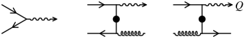
Figure 1: Real processes contributing to photon and dilepton production up to ${\cal O}(\alpha_{s})$. One loop virtual corrections to the first process also contribute at this order.

The leading order contribution to the dilepton rate is obtained from the one-loop contribution to the polarization tensor, and corresponds to the Drell-Yan process illustrated by the diagram on the left of fig. 1 (only the production of the virtual photon is represented). It was evaluated for a QGP in McLerT1 .

2.2 First perturbative corrections

The corrections of order ${\cal O}(\alpha_{s})$, where $\alpha_{s}\equiv g^{2}/4\pi$, with $g$ the QCD gauge coupling, correspond to the two diagrams in the right of figure 1. Their calculation reveals two problems. For the dilepton rate ($Q^{2}>0$) in a plasma of massless quarks and gluons, each individual contribution to eq. (3) contains a mass singularity, and it is only after a careful summation of all the real and virtual corrections that one gets a finite result BaierPS2 ; AltheAB1 ; AltheR1 . This is nothing but a manifestation of the KLN theorem LeeN1 ; Kinoshita . In the case of real photons ($Q^{2}\to 0^{+}$) a new singularity appears, with contributions of the form

$${\rm Im}\,\Pi_{\rm ret}(\omega,{\boldsymbol{q}})\propto\alpha\alpha_{s}\ln(\omega T/Q^{2})$$ (5)

at small $Q^{2}$. The singularity originates from the presence of intermediate massless quarks (the “vertical” propagators in the two diagrams in the right of fig. 1). As we shall see, plasma effects induce effective masses and cure part of the difficulty.

2.3 Scales and degrees of freedom in a quark-gluon plasma

At this point it is useful to recall some basic properties of a quark-gluon plasma in the weak coupling regime, i.e. at sufficiently high temperature Blaizot:2001nr . This regime is characterized by a hierarchy of momentum scales. Most of the plasma particles have momenta of the order of the temperature $T$, and since their density is of order $T^{3}$, $T$ is also the inverse of the inter-particle distance. Besides, collective excitations can develop in the system. Such collective phenomena are particularly important at the scale $gT$, where $g$ is the gauge coupling (the reason why these excitations are called collective is that, when $g\ll 1$, their wavelength $\sim 1/gT$ is large compared to the inter-particle distance $\sim 1/T$, so that many particles participate in the excitation). Systematic corrections to the propagation and interactions of such collective excitations involve the resummation of the so-called “hard thermal loops” BraatP1 ; FrenkT1 . Note that the soft collective modes also modify the spectrum of hard particles, giving them a mass that we shall refer to as $m_{\infty}$ ($\sim gT$). Finally, another scale plays an important role in a quark-gluon plasma: this is the scale $g^{2}T$ where perturbation theory breaks down because of the presence of unscreened magnetic fluctuations. The scale $g^{2}T$ characterizes also the rate of collisions with small ($\sim gT$) momentum transfer. To see that write the scattering cross section as $\sigma=\int{\rm d}q^{2}({\rm d}\sigma/{\rm d}q^{2})$, where typically ${\rm d}\sigma/{\rm d}q^{2}\sim g^{4}/q^{4}$. The collision rate is $\gamma=n\sigma$, so that, with $n\sim T^{3}$, $\gamma\sim g^{4}\,T^{3}\,\int{\rm d}q^{2}/{q^{4}}.$ The infrared divergence of the integral is cut-off by the screening mass $m_{D}$ ($\sim gT$) ($m_{D}$ is an example of a “hard thermal loop”) leaving a finite result $\gamma\sim g^{4}T^{3}/{m_{D}^{2}}\sim g^{2}T.$ This simple estimate applies when collisions involve dominantly small momentum transfer $\sim gT$. However, when calculating the effect of collisions on transport properties, the dominant collisions involve large angle scattering and the infrared cut-off is actually taking place at a larger momentum scale, of order $T$. Thus, most transport coefficients end up being of order $g^{4}T\ln(1/g)$ Baym:1990uj .

2.4 Resummation of hard thermal loops

We can now return to eq. (5) and observe that the logarithmic singularity at $Q^{2}\to 0$ is due to the exchange of a soft massless quark. Once the HTL correction is included on the quark propagator, the quark effectively acquires a mass $m_{\infty}$ of order $gT$ ( $m_{\infty}^{2}=\pi\alpha_{s}C_{f}T^{2}$ with $C_{f}\equiv(N_{c}^{2}-1)/2N_{c}$). By taking into account this thermal correction one obtains a finite photon polarization tensor KapusLS1 ; BaierNNR1 . For hard photons, it reads:

$${\rm Im}\,\Pi_{\rm ret}{}^{\mu}{}_{\mu}(\omega,{\boldsymbol{q}})=4\pi\frac{5\alpha\alpha_{s}}{9}T^{2}\left[\ln\left(\frac{\omega T}{m_{\infty}^{2}}\right)+{\rm const}\right]\;.$$ (6)

The numerical factor $5/9$ is the sum of the quark electric charges squared for $2$ flavors (u and d); for $3$ flavors (u, d and s), this factor should be replaced by $6/9$. This formula indicates how the infrared problem is cured: $Q^{2}$ in Eq. (5) is effectively replaced by $m_{\infty}^{2}$ in the logarithm as soon as $Q^{2}$ becomes small compared to $m_{\infty}^{2}$.

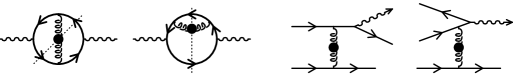
Figure 2: Processes that are promoted to ${\cal O}(\alpha_{s})$ by collinear singularities.

This, however, is not the final answer for the photon and dilepton rates at ${\cal O}(\alpha_{s})$. Indeed there are other processes, formally of higher order, which are strongly enhanced by collinear singularities and become effectively of order $\alpha_{s}$. This was first realized for soft photon production by quark bremsstrahlung AurenGKP1 ; AurenGKP2 (third diagram of fig. 2, starting from the left). The diagram on the right of figure 2 shares the same property, but contributes significantly only to hard photon production AurenGKZ1 , due to phase-space suppression in the case of soft photons. Note that a naive power counting would indicate that these two diagrams contribute to ${\cal O}(\alpha_{s}^{2})$. These two diagrams represent collision processes: they originate from cutting a loop insertion in the gluon propagator in order to get the imaginary part (the cuts are indicated by the dotted lines in the two diagrams on the left of fig. 2).

Figure 3: The virtual quark of momentum $P+Q$ emitting a real photon ($Q^{2}=0$) and an on-shell quark of momentum $P$ ($P^{2}=m^{2}$).

In order to understand the origin of the “collinear enhancement”, let us focus on the quark propagator between the quark-gluon vertex and the photon emission. The virtuality of this off-shell quark is easily estimated (see fig. 3):

$$(P+Q)^{2}-m_{\infty}^{2}=2P\cdot Q\approx\frac{m_{\perp}^{2}}{p_{z}}\,\omega\;,$$ (7)

where $m_{\perp}^{2}\equiv p_{\perp}^{2}+m_{\infty}^{2}$. Thus the virtuality of this quark can become very small if the quark is massless and the photon is emitted forward ( $p_{\perp}\to 0$). Of course, the quark thermal mass $m_{\infty}$ prevents these diagrams from being truly singular. However, contrary to the ${\cal O}(\alpha_{s})$ diagrams, the singularity is here linear instead of logarithmic, and brings a factor $T^{2}/m_{\infty}^{2}\sim 1/\alpha_{s}$. Combined with the $\alpha_{s}^{2}$ that comes from the vertices, the singularity turns the contribution of these diagrams into an order ${\cal O}(\alpha_{s})$ contribution. This was evaluated in AurenGKP2 and AurenGKZ1 (see also Mohan2 and SteffT1 where an erroneous factor $4$ was pointed out), and a closed expression was obtained in AurenGZ4 ; AurenGZ3 . The result is of the form:

$${\rm Im}\,\Pi_{\rm ret}{}^{\mu}{}_{\mu}(\omega,{\boldsymbol{q}})={\rm const\ }\alpha\alpha_{s}\left[\pi^{2}\frac{T^{3}}{\omega}+\omega T\right]\;.$$ (8)

In this formula, the term in $1/\omega$ dominates for soft photons and comes from the bremsstrahlung diagram, while the term in $\omega$ comes from the second diagram and dominates the rate of very hard photons ($\omega\gg T$).

It is worth mentioning that the purely numerical prefactor (not written explicitly in the previous formula) is a function of the ratio of the quark thermal mass $m_{\infty}$ to the gluon Debye mass $m_{{}_{D}}$. In the HTL approximation, this ratio is a constant independent of the coupling and temperature, that depends only on the number of colors and flavors; for $3$ colors and $N_{f}$ flavors, this ratio is $m_{\infty}/m_{{}_{D}}=\sqrt{2/(6+N_{f})}$.

This enhancement due to a quasi-collinear emission of the photon also occurs for the emission of virtual photons with a small invariant mass ($Q^{2}\equiv\omega^{2}-{\boldsymbol{q}}^{2}\ll\omega^{2}$), but becomes less and less important when the photon invariant mass increases. For virtual photons with vanishing momentum (i.e. for which the invariant mass is maximal, at a given energy), the two-loop diagrams contribute only at the order $g^{3}$ Aurenche:2003ac , instead of $g^{2}$ for real photons.

2.5 LPM resummation

The collinear enhancement that we have identified on some of the order $\alpha_{s}^{2}$ processes affects in fact an infinite set of processes. In order to explain the issue in physical terms, it is convenient to introduce the concept of photon formation time. Let us return to the process in figure 3. The photon formation time can be identified with the lifetime of the virtual quark, which is itself related to its virtuality by the uncertainty principle. A simple calculation gives:

$$\delta E=q+E_{p}-E_{p+q}\approx\frac{m_{\perp}^{2}}{2}\frac{\omega}{p_{z}(p_{z}+\omega)}\;,$$ (9)

where the 3-momentum of the photon defines the longitudinal axis. The formation time is $t_{{}_{F}}=1/\delta E$. The collinear enhancement in the diagrams of figure 2, due to the small virtuality of the quark that emits the photon, can be rephrased in terms of the large photon formation time. Typically, in a quark-gluon plasma, we have $m_{\perp}^{2}\sim g^{2}T^{2}$, while $p_{z}\sim T$, so that $\delta E$ in eq. (9) is $\delta E\sim g^{2}T$ for $\omega\sim T$. That is, the photon formation time is of the same order of magnitude or larger than the quark mean free path between two soft collisions, i.e. $t_{{}_{F}}\sim 1/\gamma$, where $\gamma\sim g^{2}T$ is the collision rate estimated earlier. Note that the estimate done earlier is indeed the relevant collision time scale for the production of photons almost collinear with the charge particle, that is with a typical transverse momentum of order $gT$: this is the kinematical condition leading to the enhancement that we are discussing (by “enhancement”, we mean, as earlier, the phenomenon by which higher order diagrams turn out to contribute at the same order as a given elementary process). The sensitivity to the collisional width found in AurenGZ2 occurs in the same kinematical conditions. When the mean free path becomes of the order of, or smaller than the photon formation time, the effects of multiple collisions on the production process can no longer be ignored. The result of such multiple scattering is to reduce the rate compared to what it would be if all collisions could be treated as independent source of photon production. This phenomenon is known as the Landau Pomeranchuk Migdal (LPM) effect LandaP1 ; LandaP2 ; Migda1 .

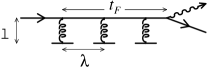
Figure 4: Diagram illustrating the conditions under which multiple collisions need to be taken into account in the photon or dilepton production process: $l$ is the typical range of the interaction producing the collisions; $\lambda$ is the mean free path, and $t_{F}$ the photon formation time.

While the early treatment of the multiple scattering was done in terms of kinetic equations, modern discussions used the language of quantum field theory. The multiple scattering diagrams that must be resummed are the ladder diagrams, as illustrated in figure 5 (these are the typical diagrams that are taken into account by a Boltzmann equation Blaizot:1999xk ). Cancellations between self-energy corrections and vertex corrections remove any sensitivity to the magnetic scale: physically, such cancellations reflect the fact that ultrasoft scatterings (at momentum scale softer than $gT$) are not efficient enough to produce a photon. A thorough diagrammatic analysis explaining why it is the ladder family of diagrams that needs to be resummed in order to obtain the complete leading ${\cal O}(\alpha_{s})$ photon rate is presented in ArnolMY1 .

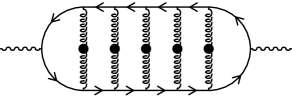
Figure 5: Resummation of ladder diagrams.

In the recent literature, the resummation of the ladder diagrams is presented as follows. The photon polarization tensor is written explicitly as ArnolMY1 ; ArnolMY2 ; ArnolMY3 :

$${\rm Im}\,\Pi_{\rm ret}{}^{\mu}{}_{\mu}(Q) \approx {\alpha N_{c}}\int_{-\infty}^{+\infty}\!\!dp_{0}\,[n_{{}_{F}}(r_{0})-n_{{}_{F}}(p_{0})]\;\frac{p_{0}^{2}+r_{0}^{2}}{(p_{0}r_{0})^{2}}$$ (10)

$$\times {\rm Re}\int\frac{d^{2}{\boldsymbol{p}}_{\perp}}{(2\pi)^{2}}\;{\boldsymbol{p}}_{\perp}\cdot{\boldsymbol{f}}({\boldsymbol{p}}_{\perp})\;,$$

with $r_{0}\equiv p_{0}+\omega$, $n_{{}_{F}}(p_{0})\equiv 1/(\exp(p_{0}/T)+1)$ the Fermi-Dirac statistical weight, and where the dimensionless function ${\boldsymbol{f}}({\boldsymbol{p}}_{\perp})$ denotes the resummed vertex connecting the quark line and the transverse modes of the photon. This function is dotted into a bare vertex, which is proportional to ${\boldsymbol{p}}_{\perp}$. The equation that determines the value of ${\boldsymbol{f}}({\boldsymbol{p}}_{\perp})$ is a Bethe-Salpeter equation that resums all the ladder corrections to the vertex ArnolMY1 ; ArnolMY2 ; ArnolMY3 :

$$\frac{i}{t_{{}_{F}}}{\boldsymbol{f}}({\boldsymbol{p}}_{\perp}) = 2{\boldsymbol{p}}_{\perp}$$

$$+ 4\pi\alpha_{s}C_{f}T\!\!\int\frac{d^{2}{\boldsymbol{l}}_{\perp}}{(2\pi)^{2}}\,{\cal C}({\boldsymbol{l}}_{\perp})\,[{\boldsymbol{f}}({\boldsymbol{p}}_{\perp}+{\boldsymbol{l}}_{\perp})-{\boldsymbol{f}}({\boldsymbol{p}}_{\perp})]\;,$$

where $t_{{}_{F}}$ is the formation time, $t_{{}_{F}}=1/\delta E$, with $\delta E$ given by eq. (9), and where the collision kernel has the following expression AurenGZ4 :

$${\cal C}({\boldsymbol{l}}_{\perp})=\frac{1}{{\boldsymbol{l}}_{\perp}^{\ 2}}-\frac{1}{{\boldsymbol{l}}_{\perp}^{\ 2}+{m^{2}_{{}_{D}}}}$$ (12)

where the two terms correspond to the exchange of a transverse and a longitudinal gluon, respectively. Note that the quark propagators should be dressed in a way compatible with the resummation performed for the vertex, in order to preserve the gauge invariance: this is the origin of the term $-{\boldsymbol{f}}({\boldsymbol{p}}_{\perp})$ under the integral in eq. (LABEL:eq:integ-f), which has the effect of resumming the collisional width on the quark propagator. From this integral equation, it is easy to see that each extra rung in the ladder contributes a correction of order $\alpha_{s}Tt_{{}_{F}}\sim{\cal O}(1)$ since $t_{{}_{F}}\sim 1/g^{2}T$. Therefore, all these corrections contribute to ${\cal O}(\alpha_{s})$ to the photon rate. Note again that the only parameters of the QGP that enter this equation are the quark thermal mass $m_{\infty}$ and the Debye screening mass $m_{{}_{D}}$.

2.6 Some numerical results

The integral equation was solved numerically in ArnolMY2 , and the results are displayed in figure 6.

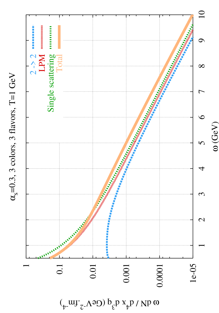
Figure 6: ${\cal O}(\alpha_{s})$ contributions to the photon production rate in a QGP. The parameters used in this plot are $\alpha_{s}=0.3$, 3 colors, 2 flavors and $T=1$ GeV. From ArnolMY2 .

In this plot, ‘LPM’ denotes the contribution of all the multiple scattering diagrams, while ‘$2\to 2$’ denotes the processes of figure 1. The single scattering diagrams (figure 2) are also given so that one can appreciate the suppression due to the LPM effect (ranging typically from 15 to 30%).

Dilepton production basically suffers from the same problems, and the solution follows the same path. Two differences are worth mentioning here. First of all, the Drell-Yan process $q\bar{q}\to\gamma^{*}\to l^{+}l^{-}$ contributes if $Q^{2}\geq 4m_{\rm q}^{2}$. The Drell-Yan process has been evaluated in McLerT1 , the $2\to 2$ processes have been evaluated in AltheR1 . In addition, virtual photons have a physical longitudinal mode that contributes to the rate of lepton pairs. In order to take this mode into account, one must introduce a scalar function $g({\boldsymbol{p}}_{\perp})$ similar to ${\boldsymbol{f}}({\boldsymbol{p}}_{\perp})$, which describes the coupling of the quark line to a longitudinal photon. This new vertex function obeys an integral equation AurenGMZ1 similar to eq. (LABEL:eq:integ-f), that resums the corrections due to multiple scatterings. This new integral equation can also be solved numerically, and the resulting dilepton rate (for the same parameters as in figure 6 and a total energy of the pair set to $\omega=5~{}$GeV) is plotted in figure 7.

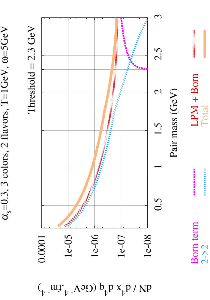
Figure 7: ${\cal O}(\alpha_{s})$ contributions to the dilepton production rate in a QGP. From AurenGMZ1 .

One can see that the multiple scattering corrections are important for all pair masses below the threshold of the Drell-Yan process. Note also that the threshold of the tree-level process is completely washed out when multiple rescatterings are resummed.

3 Lattice calculations

Attempts to calculate directly on the lattice the production rate of dileptons in a quark-gluon plasma appeared a few years ago KarscLPSW1 . What can be calculated on the lattice is the Euclidean correlator of two vector currents, $\Pi(\tau,{\boldsymbol{x}})\equiv\left<j_{\mu}(0,{\boldsymbol{0}})j^{\mu}(\tau,{\boldsymbol{x}})\right>$, where $\tau\in[0,1/T]$ is the Euclidean time. It is also easy to obtain the spatial Fourier transform at zero momentum, $\Pi(\tau,{\boldsymbol{q}}=0)$, by just summing over the spatial lattice sites. The imaginary part of the real time self-energy is then related to this object by a simple spectral representation:

$${\Pi(\tau,{\boldsymbol{q}})}=\int_{0}^{\infty}\!\!\frac{d\omega}{\pi}\,{{\rm Im}\,\Pi_{\rm ret}{}^{\mu}{}_{\mu}(\omega,{\boldsymbol{q}})}\,\frac{\cosh(\omega(\tau-1/2T))}{\sinh(\omega/2T)}\;.$$ (13)

This equation uniquely defines ${\rm Im}\,\Pi_{\rm ret}{}^{\mu}{}_{\mu}(\omega,{\boldsymbol{q}})$ if $\Pi(\tau,{\boldsymbol{q}})$ is known for all $\tau\in[0,1/T]$ and if one prescribes the behavior of the solution at large $\omega$.

However, the function $\Pi(\tau,{\boldsymbol{q}}=0)$ is known only on the discrete temporal lattice sites, which prevents us from determining uniquely ${\rm Im}\,\Pi_{\rm ret}{}^{\mu}{}_{\mu}(\omega,0)$. This problem has been reconsidered recently using the Maximum Entropy Method KarscLPSW1 ; Asakawa:2000tr , which is a way to take into account prior knowledge about the solution (positivity, behavior at the origin, etc…) in order to determine the most probable solution compatible with the lattice data and with this a priori information. The result obtained for zero momentum dileptons via this method is displayed in Fig. 8, for two different values of the temperature. Note that this is a quenched lattice simulation.

Figure 8: Lattice result for the production rate of dileptons with ${\boldsymbol{q}})=0$. From KarscLPSW1 .

This result displays several interesting properties. At energies above $4T$, the full rate is very close to the contribution of the Born term, while at energies smaller than $3T$ it drops to extremely small values. In addition, when plotted against $\omega/T$, the curves for the two temperatures fall almost on top of one another, indicating that the result scales like a universal function of $\omega/T$, at least within the errors.

The suppression at small $\omega$ has attracted a lot of interest because it contradicts expectations based on perturbation theory: the resummation of thermal masses would indeed produce a drop of the Born term because of threshold effects (see Eq. (4)), but higher order processes that do not have a threshold would fill the spectrum at small $\omega$. Also, a threshold related to the quark masses would occur at much smaller $\omega$ than $3T$, since thermal masses are typically $m\sim gT$. Finally one may question whether the accuracy of lattice calculations in the small $\omega$ regime is not spoiled by finite volume effects.

On the other hand the polarization tensor at small frequency is related to the electric conductivity Gupta:2003zh by the relation:

$$\sigma_{\rm el}=\lim_{\omega\to 0}{{{{\rm Im}\,\Pi_{\rm ret}}^{i}_{i}(\omega,{0})}/{6\omega}}.$$ (14)

From this relation, one expects ${\rm Im}\,\Pi_{\rm ret}{}^{i}_{i}(\omega,{\boldsymbol{q}}={0})\propto\omega$ when $\omega\to 0$. This implies that the static dilepton rate should diverge when $\omega\to 0$. Unless the electric conductivity in quenched QCD is nearly zero for some reason, the lattice dilepton rate disagrees with this prediction at small $\omega$. Note that ‘small’ in these considerations means an $\omega$ small enough to be in the hydrodynamical regime, i.e. $\omega\lesssim g^{4}T$. In a strong coupling theory, this regime could start as early as $\omega\sim T$.

Note that the previous argument rests on the possibility to replace ${\rm Im}\,\Pi_{\rm ret}{}^{\mu}{}_{\mu}(\omega,0)$ (involved in the calculation of the dilepton rate) by ${\rm Im}\,\Pi_{\rm ret}{}^{i}{}_{i}(\omega,0)$ (which is the quantity needed to calculate the conductivity). This is guaranteed by the Ward identity $q_{\mu}\,\Pi_{\rm ret}{}^{\mu}{}_{\mu}(\omega,0)=0$. From this it follows indeed that, unless singularities occur, $\Pi_{\rm ret}{}^{00}(\omega,0)=0$.

The electric conductivity has been calculated on the lattice by S. Gupta Gupta:2003zh , and a finite result was obtained. This calculation provides an illustration of the sensitivity of the maximum entropy method used to reconstruct the spectral functions to the prior information. Gupta’s calculation assumes explicitly that the spectral function that he wants to determine behaves linearly in $\omega$ at small $\omega$. The maximum entropy procedure yields then a finite value for the slope, i.e., a finite value for the electric conductivity. In KarscLPSW1 on the other hand, no particular assumption is made about the behavior of the spectral function at small $\omega$. For further discussion on the difficulty of extracting transport coefficients from Euclidean lattice correlators, see Aarts:2002vx ; Aarts:2002cc

4 Discussion and outlook

As of now, there are in fact arguments indicating that both the perturbative calculations and the lattice calculation are incorrect at small $\omega$. If one evaluates eq. (13) at $\tau=1/2T$, one gets a sum rule:

$$\int_{0}^{\infty}{d\omega}\,\frac{{{\rm Im}\,\Pi_{\rm ret}{}^{\mu}{}_{\mu}(\omega,{\boldsymbol{q}}=0)}}{{\sinh(\omega/2T)}}=\Pi(1/2T,0)<\infty\;,$$

This sum rule is violated by all the existing analytical weak coupling calculations (they give an infinite result). For instance, the expression in eq. (8) of the imaginary part of $\Pi$ diverges as $1/\omega$ at small $\omega$. The LPM effect would reduce the divergence to one in $1/\sqrt{\omega}$. But the expected linear behavior is not achieved in present approximations. In fact, none of the existing calculations includes correctly the dissipative effects that appear when one enters the hydrodynamical regime ($\omega\to 0$).

As for the lattice, consider again eq. (4). If one assumes that the integral is dominated by the behavior of ${\rm Im}\,\Pi$ at small $\omega$, i.e. ${\rm Im}\,\Pi^{i}_{i}(\omega,{\boldsymbol{q}}=0)\sim 6\sigma_{\rm el}\omega$, one obtains an estimate of the integral

$$\Pi_{i}^{i}(\tau={1}/{2T},{\boldsymbol{q}}=0)\approx\int_{0}^{\infty}\frac{d\omega}{\pi}\frac{\omega}{\sinh(\omega/2T)}=6\sigma_{\rm el}\pi T^{2}\;.$$

One could perhaps argue that this estimate provides in fact an upper bound for $\Pi_{i}^{i}(\tau={1}/{2T},{\boldsymbol{q}}=0)$ (if we admit that the actual function never exceeds the linear extrapolation). In order to make contact with lattice estimates, we define $C_{{}_{EM}}=4\pi\alpha\sum_{f}e_{f}^{2}$. Then we can rewrite the equation above as

$$\frac{\sigma_{\rm el}}{C_{EM}T}\approx\frac{1}{6\pi}\frac{\Pi_{i}^{i}(\tau={1}/{2T},0)}{C_{{}_{EM}}T^{3}}\;.$$ (17)

The left hand side can be obtained from Gupta’s calculation and is a number of order $7$. The right hand side is given in KarscLPSW1 , and is weakly dependent of the temperature; it is a number of order 0.12. These simple estimates suggest that the lattice calculations are not fully consistent. If we would admit that eq. (4) provides a lower bound for the electric conductivity, then the calculation in KarscLPSW1 should yield a finite $\sigma_{el}$, which is not compatible with fig. 8. It is also somewhat puzzling that the value of $\sigma$ obtained in Gupta:2003zh is so much larger than the simple estimate based on eq. (4); it would be interesting to know whether the values of $\Pi(1/2T,0)$ obtained in Gupta:2003zh agree with those given in KarscLPSW1 .

References

- [1] D.K. Srivastava, Eur. Phys. J. C 10, 487 (1999).
- [2] D.K. Srivastava, B. Sinha, Phys. Rev. C 64, 034902 (2001).
- [3] P. Huovinen, P.V. Ruuskanen, S.S. Rasanen, Phys. Lett. B 535, 109 (2002).
- [4] J. Alam, S. Sarkar, P. Roy, T. Hatsuda, B. Sinha, Annals Phys. 286, 159 (2001).
- [5] F. Gelis, Nucl. Phys. A 715, 329 (2003).
- [6] H.A. Weldon, Phys. Rev. D 28, 2007 (1983).
- [7] C. Gale, J.I. Kapusta, Nucl. Phys. B 357, 65 (1991).
- [8] F. Gelis, Nucl. Phys. B 508, 483 (1997).
- [9] L. McLerran, T. Toimela, Phys. Rev. D 31, 545 (1985).
- [10] R. Baier, B. Pire, D. Schiff, Phys. Rev. D 38, 2814 (1988).
- [11] T. Altherr, P. Aurenche, T. Becherrawy, Nucl. Phys. B 315, 436 (1989).
- [12] T. Altherr, P.V. Ruuskanen, Nucl. Phys. B 380, 377 (1992).
- [13] T. Kinoshita, J. Math. Phys. 3, 650 (1962).
- [14] T.D. Lee, M. Nauenberg, Phys. Rev. 133, 1549 (1964).
- [15] J. P. Blaizot, E. Iancu, Phys. Rept. 359, 355 (2002).
- [16] E. Braaten, R.D. Pisarski, Nucl. Phys. B 337, 569 (1990).
- [17] J. Frenkel, J.C. Taylor, Nucl. Phys. B 334, 199 (1990).
- [18] G. Baym, H. Monien, C. J. Pethick, D. G. Ravenhall, Phys. Rev. Lett. 64, 1867 (1990).
- [19] J.I. Kapusta, P. Lichard, D. Seibert, Phys. Rev. D 44, 2774 (1991).
- [20] R. Baier, H. Nakkagawa, A. Niegawa, K. Redlich, Z. Phys. C 53, 433 (1992).
- [21] P. Aurenche, F. Gelis, R. Kobes, E. Petitgirard, Phys. Rev. D 54, 5274 (1996).
- [22] P. Aurenche, F. Gelis, R. Kobes, E. Petitgirard, Z. Phys. C 75, 315 (1997).
- [23] P. Aurenche, F. Gelis, R. Kobes, H. Zaraket, Phys. Rev D 58, 085003 (1998).
- [24] A.K. Mohanty, Communication at the International Symposium in Nuclear Physics, December 18-22, 2000, Mumbai, India.
- [25] F.D. Steffen, M.H. Thoma, Phys. Lett. B 510, 98 (2001).
- [26] P. Aurenche, F. Gelis, H. Zaraket, JHEP 0205, 043 (2002).
- [27] P. Aurenche, F. Gelis, H. Zaraket, JHEP 0207, 063 (2002).
- [28] P. Aurenche, M. E. Carrington, N. Marchal, Phys. Rev. D 68, 056001 (2003).
- [29] P. Aurenche, F. Gelis, H. Zaraket, Phys. Rev. D 62, 096012 (2000).
- [30] L.D. Landau, I.Ya. Pomeranchuk, Dokl. Akad. Nauk. SSR 92, 535 (1953).
- [31] L.D. Landau, I.Ya. Pomeranchuk, Dokl. Akad. Nauk. SSR 92, 735 (1953).
- [32] A.B. Migdal, Phys. Rev. 103, 1811 (1956).
- [33] J. P. Blaizot, E. Iancu, Nucl. Phys. B 557, 183 (1999).
- [34] P. Arnold, G.D. Moore, L.G. Yaffe, JHEP 0111, 057 (2001).
- [35] P. Arnold, G.D. Moore, L.G. Yaffe, JHEP 0112, 009 (2001).
- [36] P. Arnold, G.D. Moore, L.G. Yaffe, JHEP 0206, 030 (2002).
- [37] P. Aurenche, F. Gelis, G.D. Moore, H. Zaraket, JHEP 0212, 006 (2002).
- [38] F. Karsch, E. Laermann, P. Petreczky, S. Stickan, I. Wetzorke, Phys. Lett. B 530, 147 (2002).
- [39] M. Asakawa, T. Hatsuda, Y. Nakahara, Prog. Part. Nucl. Phys. 46, 459 (2001).
- [40] S. Gupta, Phys. Lett. B 597, 57 (2004).
- [41] G. Aarts, J. M. Martinez Resco, Nucl. Phys. Proc. Suppl. 119, 505 (2003).
- [42] G. Aarts, J. M. Martinez Resco, JHEP 0204, 053 (2002).