A NEW APPROACH TO INCLUSIVE DECAY SPECTRA

The main obstacle in describing inclusive decay spectra in QCD — which, in particular, limits the precision in extrapolating the measured $\bar{B}\longrightarrow X_{s}\gamma$ rate to the full phase space as well as in extracting $|V_{ub}|$ from inclusive measurements of charmless semileptonic decays — is their sensitivity to the non-perturbative momentum distribution of the heavy quark in the meson. We show that, despite this sensitivity, resummed perturbation theory has high predictive power. Conventional Sudakov–resummed perturbation theory describing the decay of an on-shell heavy quark yields a divergent expansion. Detailed understanding of this divergence in terms of infrared renormalons has paved the way for making quantitative predictions. In particular, the leading renormalon ambiguity cancels out between the Sudakov factor and the quark pole mass. This cancellation requires renormalon resummation but involves no non-perturbative information. Additional effects due to the Fermi motion of the quark in the meson can be systematically taken into account through power corrections, which are only important near the physical endpoint. This way the moments of the $\bar{B}\longrightarrow X_{s}\gamma$ spectrum with experimentally–accessible cuts — which had been so far just parametrized — were recently computed by perturbative means. At Moriond these predictions were confronted with new data from BaBar.

1 Introduction

Experimental measurements of inclusive decays, such as $\bar{B}\longrightarrow X_{s}\gamma$ and $\bar{B}\longrightarrow X_{u}l\bar{\nu}$, cannot be performed over the whole phase space. Therefore, in order to make precision tests of the Standard Model, we must have a quantitative understanding of the spectra.

Most of the rate of these decays is associated with jet–like kinematics, where the invariant mass of the hadronic system is small. It is well known that this important region is difficult to describe theoretically $\!{}^{{\bf?},{\bf?},{\bf?}}$: the observed spectrum is directly sensitive to soft radiation off the heavy quark which is hard to disentangle from the “primordial” momentum distribution of the heavy quark in the meson. Technically, this sensitivity leads to the breakdown of the perturbative expansion in powers of $\alpha_{s}(m_{b})$ as well as that of the local Operator Product Expansion (OPE) in powers of $\Lambda/m_{b}$.

Let us consider the photon–energy spectrum in $\bar{B}\longrightarrow X_{s}\gamma$. The non-perturbative nature of this distribution is obvious from the fact that the physical endpoint is near $E_{\gamma}=M_{B}/2$, where $M_{B}$ is the meson mass, while at any order in perturbation theory — where the initial state is represented by an on-shell heavy quark — the spectrum vanishes for $E_{\gamma}>m_{b}/2$, where $m_{b}$ is the quark pole mass. In reality the quark is off shell and its Fermi motion translates into smearing  of the spectrum up to $E_{\gamma}\simeq M_{B}/2$. Given this physical picture the perturbative approach appears inappropriate. Consequently, the predominant strategy has been to parametrize the spectrum based on available data, rather than to compute it. On the other hand, since total inclusive rates, as well as their first few moments, are theoretically described by the OPE $\!{}^{{\bf?},{\bf?}}$ — and in particular, if ${\cal O}(\Lambda^{2}/m_{b}^{2})$ terms are neglected, by perturbation theory — one expects just small, computable deviations when moderate kinematic cuts are applied $\!{}^{{\bf?}}$. Progressing to more stringent cuts, resummed perturbation theory is needed. Eventually it must be complemented by non-perturbative corrections. We will show that the predictive power of resummed perturbation theory is significantly higher than it superficially appears to be.

2 The divergent nature of the perturbative expansion of spectral moments

A key ingredient in the perturbative approach to inclusive spectra is the use of moment space. Considering the $\bar{B}\longrightarrow X_{s}\gamma$ photon–energy spectrum in terms of $x\equiv 2E_{\gamma}/m_{b}$, the perturbative coefficients have singular structure at the perturbative endpoint, $x=1$. Owing to cancellation of logarithmic infrared singularities between real–emission and virtual corrections, the moments

$$\Gamma_{N}^{\hbox{\tiny PT}}\,\equiv\,\int dE_{\gamma}\left(\frac{2E_{\gamma}}{m_{b}}\right)^{N-1}\frac{d\Gamma^{{\hbox{\tiny PT}}}}{dE_{\gamma}}=\int_{0}^{1}dx\,x^{N-1}\,\frac{d\Gamma^{\hbox{\tiny PT}}(x)}{dx}$$ (1)

are infrared– and collinear–safe. $\Gamma_{N}^{\hbox{\tiny PT}}$ has a well defined perturbative expansion to all orders. This expansion, however, does not converge well. It has: (a) Sudakov logarithms, $\ln N$, that are the finite reminder in the cancellation of logarithmic infrared singularities. These logarithms appear at any order in the expansion and dominate the coefficients at large $N$ (b) infrared renormalons that reflect power–like sensitivity to soft momenta and induce factorial growth of the coefficients at large orders that renders the perturbative expansion non-summable.

To make quantitative predictions both these sources of large corrections need to be resummed. The resummation of Sudakov logarithms is possible thanks to the factorization property of matrix elements in the soft and the collinear limits. In decay spectra there are two distinct regions of phase space giving rise to infrared logarithms $\!{}^{{\bf?}}$: soft radiation with momenta of order $m/N$ from the nearly on-shell heavy quark and fragmentation of the final–state jet of mass squared $m^{2}/N$. In moment space these contribution factorize:

$$\Gamma_{N}^{\hbox{\tiny PT}}=H(m_{b})J(m_{b}^{2}/N;\mu)S_{\hbox{\tiny PT}}(m_{b}/N;\mu)\equiv H(m_{b})\times{\rm Sud}(N,m_{b}),$$ (2)

up to corrections ${\cal O}(1/N)$. Here $\mu$ is a logarithmic factorization scale. The Sudakov factor, which sums up the logs to all orders in $\alpha_{s}(m_{b})$, takes the form of an exponential:

$$\!\!\!\!{{\rm Sud}(N,m_{b})}\!\!\!\! = \!\!\!\!\exp\left\{-\sum_{n=1}^{\infty}\sum_{k=1}^{n+1}{c_{n,k}}\,{\ln^{k}N}{\left(\frac{\alpha_{s}^{\hbox{$\overline{\hbox{\tiny MS}}\,$}}(m_{b}^{2})}{\pi}\right)}^{n}\right\}\,=\,\exp\left\{\sum_{l=0}^{\infty}g_{l}(\lambda)\left(\frac{\alpha_{s}^{\hbox{$\overline{\hbox{\tiny MS}}\,$}}(m_{b}^{2})}{\pi}\right)^{l-1}\right\}\!,$$ (3)

where $\lambda\equiv\left(\beta_{0}{\alpha_{s}^{\hbox{$\overline{\hbox{\tiny MS}}\,$}}(m_{b}^{2})}/{\pi}\right)\ln N$. Note that ${{\rm Sud}(N,m_{b})}$ depends on the quark mass only through the argument of the coupling and that it does not depend on any factorization scale. The first three towers of logarithms in the exponent, i.e. $c_{n,n+1}$ — leading logs (LL), $c_{n,n}$ — next–to–leading logs (NLL) and $c_{n,n-1}$ — next–to–next–to–leading logs (NNLL) are known exactly $\!{}^{{\bf?},{\bf?}}$. The numerical values of the first few coefficients (for $N_{f}=4$) are given in Table 1. Obviously, there is problem: the coefficients increase so fast with increasing powers of $\alpha_{s}(m_{b})$ (corresponding to subleading logarithms) that the sum in the exponent cannot be determined. The result of conventional Sudakov resummation with fixed logarithmic accuracy (see Section 2.1 in Ref. $\!{}^{{\bf?}}$) is shown in Fig. 1. It does not reach perturbative stability.

$$\begin{array}[]{rrrrrrrrrr}-1.564&0.667&{\color[rgb]{0,0,1}0}&{\color[rgb]{0,0,1}0}&{\color[rgb]{0,0,1}0}&{\color[rgb]{0,0,1}0}&{\color[rgb]{0,0,1}0}&{\color[rgb]{0,0,1}0}\\ 3.837&-0.078&1.389&{\color[rgb]{0,0,1}0}&{\color[rgb]{0,0,1}0}&{\color[rgb]{0,0,1}0}&{\color[rgb]{0,0,1}0}&{\color[rgb]{0,0,1}0}\\ {\color[rgb]{1,0,0}?}&20.579&6.339&3.376&{\color[rgb]{0,0,1}0}&{\color[rgb]{0,0,1}0}&{\color[rgb]{0,0,1}0}&{\color[rgb]{0,0,1}0}\\ {\color[rgb]{1,0,0}?}&{\color[rgb]{1,0,0}?}&116.464&33.024&9.042&{\color[rgb]{0,0,1}0}&{\color[rgb]{0,0,1}0}&{\color[rgb]{0,0,1}0}\\ {\color[rgb]{1,0,0}?}&{\color[rgb]{1,0,0}?}&{\color[rgb]{1,0,0}?}&597.221&138.600&25.955&{\color[rgb]{0,0,1}0}&{\color[rgb]{0,0,1}0}\\ {\color[rgb]{1,0,0}?}&{\color[rgb]{1,0,0}?}&{\color[rgb]{1,0,0}?}&{\color[rgb]{1,0,0}?}&2859.284&548.170&78.492&{\color[rgb]{0,0,1}0}\\ {\color[rgb]{1,0,0}?}&{\color[rgb]{1,0,0}?}&{\color[rgb]{1,0,0}?}&{\color[rgb]{1,0,0}?}&{\color[rgb]{1,0,0}?}&13141.289&2129.058&247.233\\ {\color[rgb]{1,0,0}?}&{\color[rgb]{1,0,0}?}&{\color[rgb]{1,0,0}?}&{\color[rgb]{1,0,0}?}&{\color[rgb]{1,0,0}?}&{\color[rgb]{1,0,0}?}&58941.217&8238.359\\ {\color[rgb]{1,0,0}?}&{\color[rgb]{1,0,0}?}&{\color[rgb]{1,0,0}?}&{\color[rgb]{1,0,0}?}&{\color[rgb]{1,0,0}?}&{\color[rgb]{1,0,0}?}&{\color[rgb]{1,0,0}?}&260391.559\\ \end{array}$$

Table 1: The coefficients $c_{n,k}$ in Eq. (3) that are known exactly (NNLL accuracy). Rows (top to bottom) and columns (left to right) correspond to increasing powers of $n$ (power of $\alpha_{s}(m)$) and $k$ (power of $\ln N$), respectively. The three diagonals are LL, NLL and NNLL, respectively.

$$\begin{array}[]{rrrrrrrrrr}-1.56&0.67&{\color[rgb]{0,0,1}0}&{\color[rgb]{0,0,1}0}&{\color[rgb]{0,0,1}0}&{\color[rgb]{0,0,1}0}&{\color[rgb]{0,0,1}0}&{\color[rgb]{0,0,1}0}\\ 1.24&0.90&1.39&{\color[rgb]{0,0,1}0}&{\color[rgb]{0,0,1}0}&{\color[rgb]{0,0,1}0}&{\color[rgb]{0,0,1}0}&{\color[rgb]{0,0,1}0}\\ 61.17&28.32&8.28&3.38&{\color[rgb]{0,0,1}0}&{\color[rgb]{0,0,1}0}&{\color[rgb]{0,0,1}0}&{\color[rgb]{0,0,1}0}&\\ 1096.06&515.20&166.25&34.89&9.04&{\color[rgb]{0,0,1}0}&{\color[rgb]{0,0,1}0}&{\color[rgb]{0,0,1}0}\\ 20399.23&10078.43&3231.40&793.25&131.33&25.95&{\color[rgb]{0,0,1}0}&{\color[rgb]{0,0,1}0}\\ 444615.21&221481.03&73268.94&17791.58&3514.66&482.12&78.49&{\color[rgb]{0,0,1}0}\\ 11342675.74&5665794.49&1883129.50&468180.33&91361.30&15080.79&1768.50&247.23\\ 334032127.30&166960507.50&55609620.17&13867704.58&2760946.21&449959.01&63745.75&6532.65\\ \end{array}$$

Table 2: The coefficients $c_{n,k}$ in Eq. (3) computed in the large–$\beta_{0}$ limit. Columns and rows are as in Table 1.

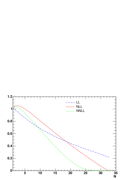
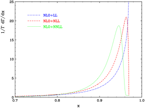
Figure 1: The moment–space Sudakov factor ${\rm Sud}(N,m_{b})$, and the corresponding differential spectrum, where the exponent is computed to LL, NLL and NNLL accuracy , as dotdashes, dashes and dots, respectively. In each case the spectrum is matched to the full NLO result for the magnetic interaction $O_{7}$. The curves end at $N\simeq 33$ and at $x\simeq 0.97$, respectively, where the Landau singularity in $g_{l}(\lambda)$ appears.

To understand the reason for this divergent behavior it is useful to consider the large–$\beta_{0}$ limit, where all the coefficients in the exponent can be computed. The numerical values of the first few coefficients (for $N_{f}=4$) in this approximation are given in Table 2. We observe that: (a) the result is similar to the full QCD matrix of Table 1; (b) further subleading logarithms have yet larger coefficients. We therefore deduce that the divergent behavior in Table 1 is related with running–coupling effects. This is a general phenomenon $\!{}^{{\bf?},{\bf?},{\bf?},{\bf?},{\bf?}}$: the large–order behavior of Sudakov exponents is dominated by infrared renormalons. The increasing coefficients of subleading logarithms build up factorial growth that renders the series non-summable. Since in the case under consideration the divergent behavior hits already at low orders it seems that any attempt to use this expansion is doomed to fail.

3 Taming the divergence by Dressed Gluon Exponentiation (DGE)

It was recently shown $\!{}^{{\bf?}}$ that, despite the divergent behavior described above, resummed perturbation theory à la DGE does lead to quantitative predictions for the $\bar{B}\longrightarrow X_{s}\gamma$ spectrum:

$$\frac{d\Gamma(E_{\gamma})}{dE_{\gamma}}=\frac{M_{B}}{2}\int_{c-i\infty}^{c+i\infty}\frac{dN}{2\pi i}\,\Gamma_{N}\,\left(\frac{2E_{\gamma}}{M_{B}}\right)^{-N}\simeq\frac{m_{b}^{{\color[rgb]{1,0,0}\hbox{\tiny PV}}}}{2}\,\int_{c-i\infty}^{c+i\infty}\frac{dN}{2\pi i}\,\,\Gamma_{N}^{{\hbox{\tiny PT},{\color[rgb]{1,0,0}\hbox{\tiny PV}}}}\,\left(\frac{2E_{\gamma}}{m_{b}^{{\color[rgb]{1,0,0}\hbox{\tiny PV}}}}\right)^{-N},$$ (6)

where the first inverse–Mellin integral is written in terms of physical spectral moments:

$$\Gamma_{N}\equiv\int dE_{\gamma}\left(\frac{2E_{\gamma}}{M_{B}}\right)^{N-1}\frac{d\Gamma}{dE_{\gamma}}=\Gamma_{N}^{{\hbox{\tiny PT},{\color[rgb]{1,0,0}\hbox{\tiny PV}}}}\,{\rm e}^{-{(N-1)\bar{\Lambda}_{{\color[rgb]{1,0,0}\hbox{\tiny PV}}}}/{M_{B}}}\,{{\cal F}((N-1)\Lambda/M_{B})},$$ (7)

with $\bar{\Lambda}_{{\color[rgb]{1,0,0}\hbox{\tiny PV}}}\equiv M_{B}-m_{b}^{{\color[rgb]{1,0,0}\hbox{\tiny PV}}}$, and $\Gamma_{N}^{{\hbox{\tiny PT},{\color[rgb]{1,0,0}\hbox{\tiny PV}}}}$ corresponds to the perturbative moments of Eq. (1), where the renormalon ambiguity is regularized using Principal Value (PV) Borel summation. In the second inverse–Mellin integral in Eq. (6) we assumed ${\cal F}\simeq 1$, an approximation that is valid away from the endpoint. Computing the spectrum by resummed perturbation theory involves:

(a)  Defining the Sudakov exponent in $\Gamma_{N}^{\hbox{\tiny PT}}$ (as an analytic function of $N$ in the complex $N$ plane) using PV Borel summation:

$$\left.{\rm Sud}(N,m_{b})\right|_{{\color[rgb]{1,0,0}\hbox{\tiny PV}}}=\exp\Bigg{\{}\frac{C_{F}}{\beta_{0}}\,{\color[rgb]{1,0,0}{\rm PV}}\int_{0}^{\infty}\frac{du}{u}T(u)\left(\frac{\Lambda^{2}}{m_{b}^{2}}\right)^{u}\times$$

$$\hskip 110.0pt\bigg{[}B_{\cal S}(u)\Gamma(-2u)(N^{2u}-1)\!-\!B_{\cal J}(u)\Gamma(-u)(N^{u}-1)\bigg{]}\Bigg{\}},$$ (8)

where $T(u)\equiv(u\delta)^{u\delta}{\rm e}^{-u\delta}/\Gamma(1+u\delta)$ with $\delta\equiv\beta_{1}/\beta_{0}^{2}$ and where the Borel transforms of the quark distribution (soft) and the jet anomalous dimensions, $B_{\cal S}(u)$ and $B_{\cal J}(u)$, respectively, are defined in Section 2.2 in Ref. $\!{}^{{\bf?}}$.

(b)  Applying the same prescription to the quark pole mass $m_{b}$ in Eq. (6) — or, equivalently to $\bar{\Lambda}$ in Eq. (7) — when computing it from the short distance mass (e.g. from $m_{b}^{\hbox{$\overline{\hbox{\tiny MS}}\,$}}$).

(c)  Performing an inverse–Mellin integral according to Eq. (6).

In general, the calculation of the Sudakov exponent by DGE differ from conventional Sudakov resummation (truncation of the sum over $l$ in Eq. (3)) in two respects. First, on the purely perturbative level, by using Eq. (3) and incorporating the exact analytic results for the anomalous dimensions in the large–$\beta_{0}$ limit $\!{}^{{\bf?}}$,

$$B_{\cal S}(u) = {\rm e}^{\frac{5}{3}u}(1-u)\,+\,{\cal O}(1/\beta_{0}),$$

$$B_{\cal J}(u) = \frac{1}{2}\,{\rm e}^{\frac{5}{3}u}\left(\frac{1}{1-u}+\frac{1}{1-u/2}\right)\frac{\sin\pi u}{\pi u}\,+\,{\cal O}(1/\beta_{0}),$$ (9)

the resummation of running–coupling contributions is performed to all orders (rather than to a given logarithmic accuracy) making the result renormalization–group invariant $\!{}^{{\bf?}}$. The power–like infrared sensitivity, which shows up in Eq. (3) through the divergence of the series, explicitly appears in Eq. (3) as Borel singularities at integer and half integer values of $u$. This brings us to the second difference, which is an important advantage of DGE, namely having a definite prescription to make power–like separation between perturbative and non-perturbative contributions. The PV prescription we choose guarantees that the perturbative moments are real valued: $\left.{\rm Sud}(N,m_{b})\right|_{{\color[rgb]{1,0,0}\hbox{\tiny PV}}}=\left[\left.{\rm Sud}(N^{\color[rgb]{1,0,1}*},m_{b})\right|_{{\color[rgb]{1,0,0}\hbox{\tiny PV}}}\right]^{\color[rgb]{1,0,1}*}$. This choice also defines the non-perturbative power corrections.

Another key property of this calculation is the exact cancellation $\!{}^{{\bf?}}$ of the leading, $u=1/2$ infrared renormalon ambiguity  between the Sudakov factor and the quark pole mass in Eq. (6). This means that the infrared sensitivity, which severely limits the accuracy of the calculation in a conventional perturbative approach (Fig. 1), is nothing else but an artifact of perturbation theory — specifically, of using an on-shell heavy quark in the initial state — and it is fully removed if renormalon resummation is applied in both the Sudakov factor and the pole mass.

To understand this cancellation consider the process–independent definition of the quark distribution in the meson as the Fourier transform of $\left<{B(P_{B})}\left|\left[\bar{\Psi}(y)\gamma^{+}\,{\Phi_{y}(0,y)}\,\Psi(0)\right]_{\mu}\right|{B(P_{B})}\right>$ with respect to $y^{-}$ where $y$ is a lightlike vector, $\Phi_{y}(0,y)$ is a Wilson line in this direction, and $\mu$ is a (dimensional–regularization) ultraviolet renormalization scale. Let us compare this distribution to its perturbative counterpart, namely the quark distribution in an on-shell heavy quark defined by the Fourier transform of $\left<{b(p_{b})}\left|\left[\bar{\Psi}(y)\gamma^{+}\,{\Phi_{y}(0,y)}\,\Psi(0)\right]_{\mu}\right|{b(p_{b})}\right>$. While the former is unambiguous, the latter involves an on-shell heavy quark external state, which is unphysical. While the moments of the latter distribution are infrared– and collinear–safe as far as logarithms are concerned, their infrared sensitivity renders them ambiguous at power accuracy. The large–$N$ limit corresponds to the replacements $iP_{B}^{+}y^{-}\longrightarrow N$ and $ip_{b}^{+}y^{-}\longrightarrow N$ in the two matrix elements, respectively. One then obtains the following relation between the two soft functions $\!{}^{{\bf?}}$:

$${S({M_{B}/N};{\mu})}=\,\underbrace{{S_{{\hbox{\tiny PT}}}({m_{b}/N};{\mu})}\,\,{\rm e}^{-{(N-1){\bar{\Lambda}}}/{M_{B}}}}_{{\rm leading\,\,renormalon\,\,cancels\,\,out}}\,{{\cal F}((N-1)\Lambda/M_{B})},$$ (10)

where power corrections on the soft scale are split into two categories: kinematic ones, which involve $\bar{\Lambda}\equiv M_{B}-m_{b}$ and therefore strongly depend on the quark–mass definition, and dynamical ones (${\cal F}$), which describe the Fermi motion of the quark in the meson. The OPE shows $\!{}^{{\bf?},{\bf?}}$ that the latter begin at ${\cal O}\Big{(}((N-1)\Lambda/M_{B})^{2}\Big{)}$. As indicated in Eq. (10) the cancellation of the leading renormalon ambiguity involves only the kinematic term and therefore it can be realized without using any non-perturbative input on the quark distribution in the meson. An explicit calculation of the quark distribution in an on-shell heavy quark in the large–$\beta_{0}$ limit  shows that the leading renormalon ambiguity in the exponent in ${S_{{\hbox{\tiny PT}}}({m_{b}/N};{\mu})}$ is indeed equal in magnitude and opposite in sign to the one in the pole mass $\!{}^{{\bf?},{\bf?}}$, confirming the cancelation in Eq. (10).

Returning to the observable, the replacement of the perturbative soft function $S_{{\hbox{\tiny PT}}}(m_{b}/N;\mu)$ in Eq. (2) by $S({M_{B}/N};{\mu})$ of Eq. (10), corresponding to the quark distribution is the meson, yields the physical spectral moments defined in Eq. (7):

$$\Gamma_{N}\,=\,H(m_{b})\,\underbrace{{\rm Sud}(N,m_{b})\,\,{\rm e}^{-{(N-1){\bar{\Lambda}}}/{M_{B}}}}_{{\rm leading\,\,renormalon\,\,cancels\,\,out}}\,{{\cal F}((N-1)\Lambda/M_{B})}.$$ (11)

These moments are free of the leading renormalon ambiguity. Given our limited knowledge of dynamic power corrections, as a first approximation it is sensible to neglect them altogether by setting ${\cal F}\simeq 1$. This leads to the second inverse–Mellin formula in Eq. (6), which is nothing but resummed perturbation theory.

In practice, the application of DGE requires evaluating the integral in Eq. (3) despite incomplete knowledge of the anomalous dimensions of both the soft and the jet functions. What we currently know about the exponent includes $\!{}^{{\bf?}}$:

• The analytic expressions in the large–$\beta_{0}$ limit $\!{}^{{\bf?}}$ for $B_{\cal S}(u)$ and $B_{\cal J}(u)$ given by Eq. (3).

• NNLO (i.e. ${\cal O}(u^{2})$) perturbative expressions in QCD $\!{}^{{\bf?},{\bf?}}$ for both $B_{\cal S}(u)$ $\!{}^{{\bf?},{\bf?}}$ and $B_{\cal J}(u)$ $\!{}^{{\bf?}}$.

• The normalization of the leading renormalon corresponding to the value of $B_{\cal S}(u)$ at $u=1/2$. This value was determined $\!{}^{{\bf?}}$, using the cancellation, based on the $u=1/2$ renormalon residue in the pole mass, which has been computed$\!{}^{{\bf?},{\bf?}}$ with a few percent accuracy from the NNLO perturbative expansion of the ratio between the pole mass and $m_{b}^{\hbox{$\overline{\hbox{\tiny MS}}\,$}}$, taking into account the known structure of the singularity $\!{}^{{\bf?}}$.

This information is sufficient $\!{}^{{\bf?}}$ to constrain the moments up to $N\sim 20$ fairly well. This is demonstrated in Fig. 2. The most important source of remaining uncertainty arises from the unknown behavior of $B_{\cal S}(u)$ away from the origin, and in particular, for $u>1/2$.

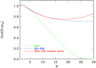
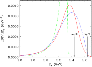
Figure 2: The moment–space Sudakov factor ${\rm Sud}(N,m_{b})$ (left), and the corresponding differential spectrum in $b\longrightarrow X_{s}\gamma$ (right) as computed by DGE with perturbative expansions of NLL (dotdashed blue line) and NNLL (full red line) accuracy. In the latter also the residue at $u=1/2$ is fixed. The DGE spectra are both matched with the full NLO. For comparison the conventional NNLL result is also shown (dashed green line).

The stability reflected in Fig. 2 stands in sharp contrast with the situation we encountered at fixed logarithmic accuracy (Fig. 1), where the leading renormalon is untamed.

Looking at Fig. 2 one immediately observes that the support properties have changed. While at any order in perturbation theory the result is identically zero for $E_{\gamma}>m_{b}/2$, upon taking the PV in Eq. (3) the distribution becomes non-zero there. The $E_{\gamma}=m_{b}/2$ boundary is a direct consequence of the assumption that the initial $b$ quark is on-shell. This inherent limitation of perturbation theory is removed upon defining the sum of the series in moment space by PV. Remarkably, the PV result tends to zero near the physical endpoint. This, together with the observed stability, suggests that in this formulation the dynamical power corrections associated with the Fermi motion (${\cal F}$), which were neglected here, are indeed small.

4 Comparison with data

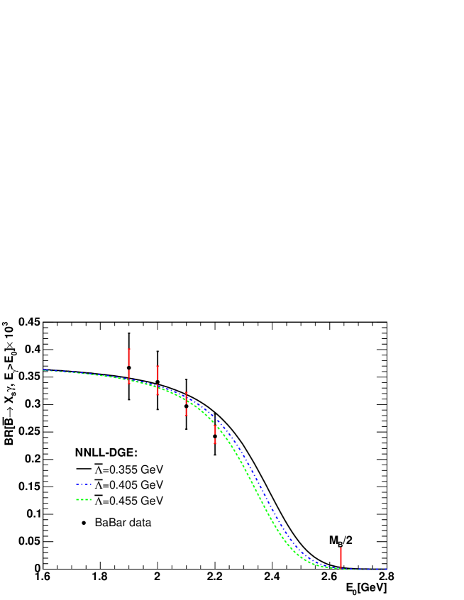
Figure 3: The partial $\bar{B}\longrightarrow X_{s}\gamma$ BF with $E_{\gamma}>E_{0}$ as computed by DGE compared with new data from BaBar. Inner and total error bars on the data points show systematic and statistical plus systematic errors (added linearly), respectively. The three theory curves shown (indicated on the plot by the corresponding values for $\bar{\Lambda}$) correspond to different input values for $m_{b}^{\hbox{$\overline{\hbox{\tiny MS}}\,$}}$ that roughly cover the uncertainty range on this parameter. Note that the overall normalization of the theoretical BF, which is fixed here to its central value of ${\rm BF}(E_{\gamma}>E_{0}=m_{b}/20)=3.73\cdot 10^{-4}$, has $\sim 10\%$ uncertainty.

Experimentally–favored observables are the partial branching fraction (BF) for $E_{\gamma}>E_{0}$,

$${\rm BF}\equiv\frac{\Gamma_{\bar{B}\longrightarrow X_{s}\gamma}(E_{\gamma}>{E_{0}})}{\Gamma_{\bar{B}\longrightarrow{\rm anything}}};\qquad\quad\Gamma(E_{\gamma}>{E_{0}})\equiv{\displaystyle\int_{{E_{0}}}dE_{\gamma}\,\frac{d\Gamma(E_{\gamma})}{dE_{\gamma}}},$$ (12)

where the cut value $E_{0}$ is above 1.8 GeV, as well as the first few spectral moments defined over similarly limited range of photon energies:

$${\Big{<}}E_{\gamma}{{{\Big{>_{{\!}_{E_{\gamma}>{E_{0}}}}}}}} \equiv \frac{1}{\Gamma(E_{\gamma}>{E_{0}})}\,{\displaystyle\int_{{E_{0}}}dE_{\gamma}\,{\frac{d\Gamma(E_{\gamma})}{dE_{\gamma}}}\,E_{\gamma}},$$ (13)

$${\Big{<}}\Big{(}{\Big{<}}E_{\gamma}{{\Big{>_{\!{}_{E_{\gamma}>{E_{0}}}}}}}-E_{\gamma}\Big{)}^{n}{\Big{>_{{\!}_{E_{\gamma}>{E_{0}}}}}} \equiv \frac{1}{\Gamma(E_{\gamma}>{E_{0}})}{\displaystyle\int_{{E_{0}}}dE_{\gamma}\,{\frac{d\Gamma(E_{\gamma})}{dE_{\gamma}}}\,\Big{(}{\Big{<}}E_{\gamma}{{\Big{>_{{\!}_{E_{\gamma}>{E_{0}}}}}}}-E_{\gamma}\Big{)}^{n}}.$$ (14)

Measurements of the average energy defined in Eq. (13), and the variance, $n=2$ in Eq. (14), with $E_{0}=1.815$ GeV were published $\!{}^{{\bf?}}$ by Belle in 2004.

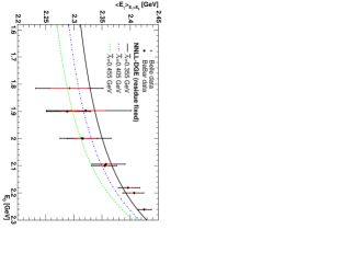
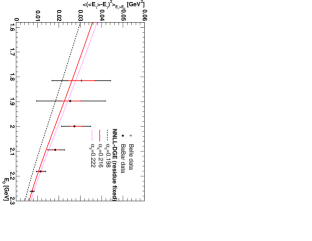
Figure 4: The first two cut moments of the $\bar{B}\longrightarrow X_{s}\gamma$ spectrum: $\left<E_{\gamma}\right>$ (left) and $\left<(\left<E_{\gamma}\right>-E_{\gamma})^{2}\right>$ (right), as a function of the minimum photon energy cut $E_{0}$, as calculated by DGE (varying $m_{b}^{\hbox{$\overline{\hbox{\tiny MS}}\,$}}$ and $\alpha_{s}$ within their error ranges), compared with data from Belle and BaBar. Inner and total error bars show systematic and statistical plus systematic errors (added linearly), respectively.

The method presented in the previous section facilitates theoretical calculation of the $\bar{B}\longrightarrow X_{s}\gamma$ spectrum, and thus also evaluation of the cut moments defined above, by purely perturbative means, so long as power corrections (${\cal F}$) can be neglected. Since these power corrections are controlled by the soft scale $m_{b}/N$, they become increasingly important with increasing $E_{0}$. In order to test the theory and, eventually, determine these power corrections it is therefore useful $\!{}^{{\bf?}}$ to compare the theoretical calculation with data as a function of $E_{0}$. Such comparison was done for the first time during the Moriond meeting, following the talk by J.J. Walsh $\!{}^{{\bf?}}$ who presented new (and preliminary) results from Babar; see Figs. 3 and 4.

5 Conclusions

We presented a new approach to inclusive decay spectra in QCD and its application to the $\bar{B}\longrightarrow X_{s}\gamma$ spectrum. Our method, Dressed Gluon Exponentiation, incorporates renormalon resummation as well as Sudakov resummation and uses the PV prescription to separate between computable perturbative contributions and non-perturbative power corrections, which become important near the endpoint.

We have shown that, despite the apparent infrared sensitivity which shows up as divergence of the perturbative expansion in Eq. (3), the predictive power of resummed perturbation theory is high. This is reflected, for example, in the stability of the DGE result shown in Fig. 2. A key property underlying this predictive power is the exact cancellation of the leading infrared renormalon ambiguity $\!{}^{{\bf?}}$. This cancellation can be understood as a manifestation of the infrared– and collinear–safety of the physical spectral moments at power accuracy.

In the calculation of the spectrum by Eq. (6) the leading renormalon cancellation is realized by using the same prescription when defining the sum in the Sudakov exponent and when computing the quark pole mass which sets the overall energy scale. Renormalon resummation in both these quantities is of course imperative for this cancellation to take place. The final result for the spectrum is prescription independent as far as this leading renormalon is concerned. Having neglected higher power corrections on the soft scale, our result does depend on using the PV prescription for higher renormalon singularities. While we do not assign to the chosen regularization any physical meaning, we find the PV prescription particularly useful. Specifically, the PV–regularized spectrum shares the following key properties with the physical spectrum: (a) the moments are real valued, (b) the resummed spectrum smoothly extends beyond the perturbative endpoint and, quite remarkably, tends to zero for $E_{\gamma}=\left(m_{b}+{\cal O}(\Lambda)\right)/2$, close to $M_{B}/2$. This suggest that in this formulation power corrections are indeed small.

Finally, as shown in Figs. 3 and 4, there is good agreement between the theoretical predictions and data from the B factories for both the partial BF and the first two spectral moments over the entire range of cuts where data is available. Fits can readily be performed to measure $m_{b}^{\hbox{$\overline{\hbox{\tiny MS}}\,$}}$ and to put bounds on the dynamical power corrections, which were so far neglected in this approach. Finally, this successful comparison with data shows that prospects are good for precision determination of $V_{ub}$ from charmless semileptonic decays using DGE.

References

References

- [1] M. Neubert, Phys. Rev. D49 (1994) 4623; [hep-ph/9312311]. Phys. Rev. D49 (1994) 3392 [hep-ph/9311325].
- [2] I. I. Y. Bigi, M. A. Shifman, N. G. Uraltsev and A. I. Vainshtein, Int. J. Mod. Phys. A9 (1994) 2467 [hep-ph/9312359].
- [3] S. W. Bosch, B. O. Lange, M. Neubert and G. Paz, Nucl. Phys. B699 (2004) 335 [hep-ph/0402094].
- [4] B. Blok, L. Koyrakh, M. A. Shifman and A. I. Vainshtein, Phys. Rev. D49 (1994) 3356 [Erratum-ibid. D50 (1994) 3572] [hep-ph/9307247].
- [5] A. V. Manohar and M. B. Wise, Phys. Rev. D49 (1994) 1310 [hep-ph/9308246].
- [6] D. Benson, I. I. Bigi and N. Uraltsev, Nucl. Phys. B710, 371 (2005) [hep-ph/0410080].
- [7] G. P. Korchemsky and G. Sterman, Phys. Lett. B340, 96 (1994) [hep-ph/9407344].
- [8] J. R. Andersen and E. Gardi, “Taming the B X/s gamma spectrum by dressed gluon exponentiation,” [hep-ph/0502159].
- [9] E. Gardi, JHEP 0502 (2005) 053 [hep-ph/0501257].
- [10] E. Gardi and J. Rathsman, Nucl. Phys. B609 (2001) 123 [hep-ph/0103217]; Nucl. Phys. B638 (2002) 243 [hep-ph/0201019].
- [11] E. Gardi, Nucl. Phys. B622 (2002) 365 [hep-ph/0108222].
- [12] M. Cacciari and E. Gardi, Nucl. Phys. B664 (2003) 299 [hep-ph/0301047].
- [13] E. Gardi and R. G. Roberts, Nucl. Phys. B653, 227 (2003) [hep-ph/0210429].
- [14] E. Gardi, JHEP 0404, 049 (2004) [hep-ph/0403249].
- [15] M. Beneke and V. M. Braun, Nucl. Phys. B426, 301 (1994) [hep-ph/9402364].
- [16] I. I. Y. Bigi, M. A. Shifman, N. G. Uraltsev and A. I. Vainshtein, Phys. Rev. D50, 2234 (1994) [hep-ph/9402360].
- [17] G. P. Korchemsky and G. Marchesini, Nucl. Phys. B406 (1993) 225 [hep-ph/9210281].
- [18] M. Beneke, V. M. Braun and V. I. Zakharov, Phys. Rev. Lett. 73 (1994) 3058 [hep-ph/9405304].
- [19] A. Pineda, JHEP 0106 (2001) 022 [hep-ph/0105008]; T. Lee, JHEP 0310, 044 (2003) [hep-ph/0304185]; G. Cvetic, J. Phys. G 30 (2004) 863 [hep-ph/0309262].
- [20] M. Beneke, Phys. Lett. B344 (1995) 341 [hep-ph/9408380].
- [21] P. Koppenburg et al. [Belle Coll.], Phys. Rev. Lett. 93 (2004) 061803 [hep-ex/0403004].
-
[22]
J.J. Walsh [BaBar Coll.] “Semileptonic and EW Penguin Decay
Results from BaBar”, Talk at the XXXXth Rencontres de Moriond QCD
and Hadronic Interactions La Thuile, Italy March 12 – March 19,
2005.
http://moriond.in2p3.fr/QCD/2005/Index.html