Abstract

The complete set of two-loop electroweak corrections to the decay width of the Higgs boson into two photons is presented. Two-loop contributions involving weak bosons and the top quark are computed in terms of an expansion in the Higgs external momentum. Adding these results to the previously known light fermion contributions, we find that the total electroweak corrections for a Higgs boson with 100 GeV $\lesssim m_{H}\lesssim$ 150 GeV are moderate and negative, between $-4\%\lesssim\delta_{EW}\lesssim 0\%$. Combination with the QCD corrections, which are small and positive, gives a total correction to the one-loop results of $|\delta_{EW+QCD}|\lesssim 1.5\%$.

1 Introduction

Understanding the mechanism of electroweak symmetry breaking (EWSB) is one of the main quests of the whole high energy physics community. The electroweak precision data collected at LEP and SLD in combination with the direct top-quark mass measurement at the Tevatron, have strongly constrained the range of possible scenarios and hinted to the existence of a light scalar particle. Both in the standard model (SM) and in its minimal supersymmetric extensions (MSSM), the $W$ and $Z$ bosons and fermions acquire masses by coupling to the vacuum expectation value(s) of scalar SU(2) doublet(s), via the so-called Higgs mechanism. The striking prediction of such models is the existence of at least one scalar state, the Higgs boson. Within the SM, LEP has put a very strong lower bound to the Higgs mass, $m_{\scriptscriptstyle H}>114$ GeV [1], and has contributed to build up the indirect evidence that the Higgs boson should be relatively light with a high probability for its mass to be below 250 GeV. In the MSSM the experimental lower mass bounds for the lightest state are somewhat weaker but internal consistency of the theory predicts an upper bound of 140-150 GeV at most [2].

In this mass intermediate range, $80\lesssim m_{H}\lesssim 130$ GeV, coupling to photons even though loop-suppressed and therefore small, is phenomenologically of great importance. At hadron colliders, the decay into two photons provides a very clean signature for the discovery in the gluon-gluon fusion production [3], for the measurements of the couplings in the vector-boson fusion channel [4] and, depending on the achievable integrated luminosity, also in the $WH,ZH$, and $t\bar{t}H$ associated productions. While none of the above measurements alone can provide information on the partial width (what is measured is $\sigma(pp\to H)\cdot$ Br$(H\to\gamma\gamma)$), their combination with signals in other decay modes, will allow a determination of the total width of the Higgs and of the couplings with a precision of 10-40% [5]. A much better determination of the Higgs width into two photons could be achieved at a $e^{+}e^{-}$ linear collider, via the fusion process $\gamma\gamma\to H$, with the photons generated by Compton-back scattering of laser light [6, 7]. In this case, it has been shown that $\sigma(\gamma\gamma\to H)\cdot$ Br$(H\to b\bar{b})$ could be measured to a precision of a few percents [8], providing an almost direct determination of the width of $H\to\gamma\gamma$ (the Br$(H\to b\bar{b})$ is large for intermediate Higgs masses and therefore quite insensitive to the total width).

In view of a precise experimental determination of the $H\to\gamma\gamma$ coupling, it is legitimate to ask how well the width can be predicted in the SM and how sensitive to the effects of new physics this quantity might be. The latter question has been the subject of several studies [9, 10, 11]. In general, it is found that corrections to the Higgs width into photons due to physics beyond the SM are moderate, ranging up to tens of percent.

The SM prediction for $\Gamma(H\to\gamma\gamma)$ includes the original one-loop computation [12] supplemented by the complete two-loop QCD corrections to one-loop top contribution [13] and the two-loop electroweak corrections evaluated in the large top-mass [14, 15] and large Higgs-mass scenarios [16]. Recently, also the two-loop contribution to $\Gamma(H\to\gamma\gamma)$ induced by the light fermion has been computed [17].

In this work we present the calculation of the two-loop electroweak corrections involving the weak bosons and the top quark which, together with the previously known contributions due to the light fermions [17], completes the two-loop determination of the $H\to\gamma\gamma$ coupling. Our investigation applies to the Higgs mass range up to the $2\,m_{\scriptscriptstyle W}$ threshold covering the by far most interesting $m_{\scriptscriptstyle H}$ region from a phenomenological point of view. The paper is organized as follows. In Section 2, we illustrate the technical details of the calculation focusing on the renormalization procedure employed. In Section 3 we discuss the numerical results and combine them with the known two-loop EW light fermion [17] and two-loop QCD corrections [13]. We collect our conclusions in Section 4.

2 Outline of the calculation

The general structure of the amplitude for the decay of a Higgs particle into two photons of polarization vectors $\epsilon_{\mu}(q_{1})$ and $\epsilon_{\nu}(q_{2})$, can be written as:

$$T^{\mu\nu}=q_{1}^{\mu}\,q_{1}^{\nu}\,T_{1}+q_{2}^{\mu}\,q_{2}^{\nu}\,T_{2}+q_{1}^{\mu}\,q_{2}^{\nu}\,T_{3}+q_{1}^{\nu}\,q_{2}^{\mu}\,T_{4}+(q_{1}\cdot q_{2})\,g^{\mu\nu}\,T_{5}+\epsilon^{\mu\nu\rho\sigma}\,q_{1\rho}\,q_{2\sigma}\,T_{6}\,.$$ (1)

Abelian gauge invariance requires that $T_{1}=T_{2}=0$ and $T_{4}=-T_{5}$; the form factor $T_{3}$ does not contribute for on-shell photons. $T_{6}$ can be generated at the two-loop level, but it has vanishing interference with the one-loop result.

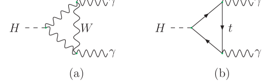
Figure 1: Representative diagrams of the one-loop contributions to $H\to\gamma\gamma$. Diagram (a) represents the bosonic contributions where the photons couple to charged bosons, unphysical scalars and ghosts. In diagram (b) the Higgs couples to the fermion line so that only heavy quarks give a non-negligible contribution.

The corresponding partial decay width can be written as:

$$\Gamma\left(H\rightarrow\gamma\,\gamma\right) = \frac{G_{\mu}\alpha^{2}\,m_{\scriptscriptstyle H}^{3}}{128\,\sqrt{2}\,\pi^{3}}\left|{\cal F}\right|^{2}\,.$$ (2)

Due to the absence of a tree-level Higgs-photon-photon coupling the lowest order contribution arises at one-loop via $W$ boson and fermion virtual effects, see Fig. 1, the latter almost entirely due to the top quark with a small correction from the bottom. The lowest order contribution was computed several years ago [12]. Neglecting the bottom part it is given by:

$${\cal F}^{1l} = {\cal F}^{1l}_{\scriptscriptstyle W}+{\cal F}^{1l}_{t}~{},$$ (3)

$${\cal F}^{1l}_{\scriptscriptstyle W} = 2\,(1+6\,w_{\scriptscriptstyle H})-12\,w_{\scriptscriptstyle H}\,(1-2\,w_{\scriptscriptstyle H})\,H\left(-r,-r;-\frac{1}{w_{\scriptscriptstyle H}}\right)~{},$$ (4)

$${\cal F}^{1l}_{t} = -4Q_{t}^{2}N_{c}\,t_{\scriptscriptstyle H}\,\left[2-(1-4\,t_{\scriptscriptstyle H})\,H\left(-r,-r;-\frac{1}{t_{\scriptscriptstyle H}}\right)\right]~{},$$ (5)

where $w_{\scriptscriptstyle H}\equiv m_{\scriptscriptstyle W}^{2}/m_{\scriptscriptstyle H}^{2}$, $t_{\scriptscriptstyle H}\equiv m_{t}^{2}/m_{\scriptscriptstyle H}^{2}$, $N_{c}$ is the color factor and

$$H(-r,-r;x)=\frac{1}{2}\log^{2}\left(\frac{\sqrt{x+4}-\sqrt{x}}{\sqrt{x+4}+\sqrt{x}}\right)~{}.$$ (6)

In Eqs. (4-6) we have expressed the result of the loop integration in terms of one of the Generalized Harmonic Polylogarithms (GHPLs) [18] of weight two employing the notation of Ref. [19]. At one loop the contribution of light fermions is suppressed by the smallness of both the Yukawa coupling and the kinematical mass. When the Higgs is light, the top and the bosonic contributions can be expanded in $h_{4w}\equiv m_{H}^{2}/(4\,m_{\scriptscriptstyle W}^{2})$ and $h_{4t}\equiv m_{H}^{2}/(4\,m_{t}^{2})$ with the result

$${\cal F}^{1l}_{{\scriptscriptstyle W}}=7+\frac{22}{15}h_{4w}+\frac{76}{105}h_{4w}^{2}+\frac{232}{525}h_{4w}^{3}+{\cal O}(h_{4w}^{4})\,,$$ (7)

and

$${\cal F}^{1l}_{t}=-Q_{t}^{2}N_{c}\left(\frac{4}{3}+\frac{14}{45}h_{4t}+\frac{8}{63}h_{4t}^{2}+\frac{104}{1575}h_{4t}^{3}+{\cal O}(h_{4t}^{4})\right)\,.$$ (8)

From the above expansions it is manifest that both contributions approach constant values (${\cal F}^{1l}_{\scriptscriptstyle W}\rightarrow 7,\,{\cal F}^{1l}_{t}\rightarrow-4/3Q_{t}^{2}N_{c}$) for mass of the particle inside the loop much heavier than $m_{\scriptscriptstyle H}$. Furthermore, the $W$ and top one-loop parts are of opposite sign and therefore interfere destructively, the former giving the dominant contribution for light Higgs masses.

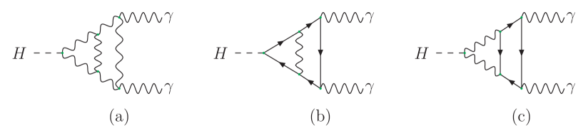
Figure 2: The three classes of two-loop diagrams contributing to $H\to\gamma\gamma$. Diagram (a) represents purerely bosonic contributions, which are the corrections to the corresponding diagram (a) of Fig. 1. Diagrams (b) and (c) are both corrections to the diagram (b) of Fig. 1. Leptons and light quarks start contributing at two loops through diagrams of type (c).

At the two-loop level the electroweak corrections to $H\rightarrow\gamma\gamma$ can be divided in two subsets: the corrections induced by the light (assumed massless) fermions and the rest which involves heavy particles in the loops that can be further divided in a purely bosonic contribution and a contribution involving third generation quarks:

$${\cal F}^{2l} = {\cal F}^{2l}_{heavy}+{\cal F}^{2l}_{lf}$$ (9)

$$= {\cal F}^{2l}_{\scriptscriptstyle W}+{\cal F}^{2l}_{t}+{\cal F}^{2l}_{lf}.$$

In Fig. 2 we draw one representative diagram for each type of contribution in ${\cal F}^{2l}$. We notice that diagrams of type (c) can also contribute to ${\cal F}^{2l}_{t}$ when in the internal lines a top quark is exchanged. In Eq. (9) the last contribution is very different from the others two because it involves particles that do not appear in the one-loop calculation. Instead, as shown in Fig. 2c, at the two-loop level, the light fermions may couple to the $W$ or $Z$ bosons which in turn can directly couple to the Higgs particle. The light fermion corrections form a gauge invariant subset of ${\cal F}^{2l}$ and have been computed exactly in Ref. [17], where the analytic result has been expressed in terms of GHPLs. In that analysis diagrams where the bottom quark, which is assumed massless, is present together with the $Z$ boson were also included.

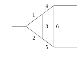
Figure 3: Diagram for studying the cut structure of the amplitude.

As anticipated, in this paper we present the result for ${\cal F}^{2l}_{\scriptscriptstyle W}$ and ${\cal F}^{2l}_{t}$ for Higgs mass values in the intermediate region. Before discussing in detail the structure of the calculation we notice that for such a values of the Higgs mass the computation of the one-particle irreducible (1PI) two-loop diagrams can be obtained via an ordinary Taylor expansion in the variable $q_{4w}\equiv q^{2}/(4\,m_{\scriptscriptstyle W}^{2})$ where $q$ is the momentum carried by the Higgs. To appreciate this point, we discuss the structure of the cuts in the Feynman diagrams that contribute to ${\cal F}^{2l}_{heavy}$. As an example we take the topology drawn in Fig. 3, that is actually present in both sets. In the ${\cal F}^{2l}_{\scriptscriptstyle W}$ part, the diagrams corresponding to Fig. 3 exhibit a first cut through lines (1,2), (4,5) and (1,3,5) (or (2,3,4)) at $q^{2}=4m_{\scriptscriptstyle W}^{2}$ because the only massless particle in the purely bosonic contribution is the photon (we work in the Feynman gauge) that in this specific example can only appear in position 3 (see Fig. 2(a) ). With respect to ${\cal F}^{2l}_{t}$ it seems that the diagrams of Fig. 3 can develop a cut at $q^{2}=0$ through lines (4,5) when they represent a bottom quark (see Fig. 2(c)). However, as discussed in detail in Ref. [20] this cut is actually not present because of the helicity structure of the diagram. Then, in this set the first cut arises again at $q^{2}=4m_{\scriptscriptstyle W}^{2}$ through lines (1,2). We notice that the same topology is actually present also in the light fermion contribution. In this case because lines 3 and 5 should be taken both massless the diagrams develop a cut at $q^{2}=m_{\scriptscriptstyle W}^{2}$ through lines (1,3,5). Indeed the explicit expression for ${\cal F}^{2l}_{lf}$ given in Ref. [17] in terms of the GHPLs contains an imaginary part when $q^{2}>m_{\scriptscriptstyle W}^{2}$.

To evaluate ${\cal F}^{2l}_{\scriptscriptstyle W}$ and ${\cal F}^{2l}_{t}$ we find it convenient to employ the Background Field Method (BFM) quantization framework. The BFM is a technique for quantizing gauge theories [21, 22] that avoids the complete explicit breaking of the gauge symmetry. One of the salient features of this approach is that all fields are split in two components: a classical background field $\hat{V}$ and a quantum field $V$ that appears only in the loops. The gauge-fixing procedure is achieved through a non linear term in the fields that breaks the gauge invariance only of the quantum part of the lagrangian, preserving the gauge symmetry of the effective action with respect to the background fields. Thus, in the BFM framework some of the vertices in which background fields are present are modified with respect to the standard $R_{\xi}$ gauge ones. The complete set of BFM Feynman rules for the SM can be found in Ref. [23].

In the BFM Feynman gauge (BFG) the heavy two-loop contributions to the Higgs decay into two photons can be organized as

$${\cal F}^{2l}_{heavy} = K_{r}{\cal F}^{1l}+{\cal F}^{2l}|_{\rm 1PI}\,,$$ (10)

where each individual term is finite. In Eq. (10) the factor $K_{r}$, whose explicit expression is given in Ref. [20], takes into account the reducible contribution, i.e., the Higgs wave function renormalization plus the expansion of the bare coupling $g_{0}/m_{{\scriptscriptstyle W}_{0}}$ ($g$ being the $SU(2)$ coupling) in terms of $\mu$-decay constant, or

$$K_{r}\equiv\frac{1}{2}\left[\frac{A_{{\scriptscriptstyle W}{\scriptscriptstyle W}}(0)}{m_{\scriptscriptstyle W}}-V-B+\delta Z_{\scriptscriptstyle H}\,\right]\,,$$ (11)

where $A_{{\scriptscriptstyle W}{\scriptscriptstyle W}}(0)$ is the transverse part of the $W$ self-energy at zero momentum transfer, the quantities $V$ and $B$ represent the vertex and box corrections in the $\mu$-decay amplitude and $\delta Z_{\scriptscriptstyle H}$ is related to the Higgs field wave function renormalization through

$$H_{0}=\sqrt{Z_{\scriptscriptstyle H}}H\simeq\left(1+\frac{1}{2}\,\delta Z_{\scriptscriptstyle H}\right)H~{}~{}.$$ (12)

It is known [23, 24] that the BFG self-energies coincide with those obtained in the standard $R_{\xi}$ gauges via the pinch technique (PT) procedure [25]. The PT is a prescription that combines the conventional self-energies with specific parts of the vertex and box diagrams, the so-called pinch parts, such that the resulting PT self-energies are gauge-independent in the class of $R_{\xi}$ gauges. Once in Eq. (11) the Higgs wave-function term $\delta Z_{\scriptscriptstyle H}$ is intended as the corresponding PT quantity [26], then the two terms in Eq. (10) are actually finite and gauge-invariant in the $R_{\xi}$ gauges. Eq. (10) can be further divided into a purely bosonic (no fermionic line present) and a top part

$${\cal F}^{2l}_{{\scriptscriptstyle W}} = K_{\scriptscriptstyle W}{\cal F}^{1l}_{\scriptscriptstyle W}+{\cal F}^{2l}_{{\scriptscriptstyle W}}|_{\rm 1PI}\,,$$ (13)

$${\cal F}^{2l}_{t} = (K_{t}{\cal F}^{1l}+K_{\scriptscriptstyle W}{\cal F}^{1l}_{t})+{\cal F}^{2l}_{t}|_{\rm 1PI}\,,$$ (14)

where each term is separately finite and gauge independent. $K_{{\scriptscriptstyle W},t}$ are the purely bosonic and the top part of $K_{r}$ respectively, with $K_{\scriptscriptstyle W}+K_{t}=K_{r}$, and ${\cal F}^{2l}_{{\scriptscriptstyle W},t}|_{\rm 1PI}$ are the two-loop 1PI corrections plus the counterterms contribution (apart from the $g_{0}/m_{{\scriptscriptstyle W}_{0}}$ factor).

The evaluation of ${\cal F}^{2l}|_{\rm 1PI}$ has been performed via a Taylor series in $q_{4w}$ through $O(q_{4w}^{4})$ terms. The 1PI diagrams ($\sim 1700)$ have been generated using the program FeynArts [27]. The relevant form factor, $T_{5}$, has been extracted via the use of a standard projector. The Taylor expansion of the scalar amplitudes has been obtained employing an algorithm developed by O.V. Tarasov [28]. The resulting two-loop vacuum integrals have been analytically evaluated using the expressions of Ref. [29]. As a check of our computation we have verified the abelian gauge invariance, i.e., $T_{1}=T_{2}=0$. We notice that while in the standard $R_{\xi}$ gauges this property is verified only by the on-shell amplitude, i.e., when $q^{2}=m_{\scriptscriptstyle H}^{2}$, in the BFG it is satisfied also in the off-shell case, i.e., for arbitrary value of $q^{2}$.

The tadpole diagrams and the counterterm contribution in ${\cal F}^{2l}|_{\rm 1PI}$ deserve a detailed discussion. In Eq. (2), the width is expressed in terms of $G_{\mu}$ and $\alpha(0)=1/137.036\dots$, a choice that fixes the renormalization of $g$ and of the photon coupling. The other parameters that require a renormalization prescription are the mass of $W$ boson, of its unphysical counterpart, $\phi$, and the corresponding ghost particle, $c$, as well as that of the top quark. Furthermore, the quartic coupling in the scalar potential, $\lambda$, should also be renormalized. In fact $\lambda$ enters in the $\phi^{+}\phi^{-}h$ coupling that is given by $2\lambda v$, $v$ being the v.e.v. of Higgs field.

We employ on-shell masses for the physical particles. Then $\delta v$ is fixed in terms of $\delta g$ and $\delta m_{\scriptscriptstyle W}^{2}$. In the Feynman gauge we use, the mass renormalization for the $c$ and $\phi$ fields can be chosen to be equal to that of the $W$ mass, i.e., $\delta m^{2}_{c}=\delta m_{\scriptscriptstyle W}^{2},\>\delta m^{2}_{\phi}=\delta m_{\scriptscriptstyle W}^{2}$.

We eliminate the tadpole diagrams by fixing the tadpole counterterm to cancel them. This implies that the renormalization of the $\phi$ mass should be augmented by the tadpole contribution, $\delta\tau$, i.e.,

$$\delta m^{2}_{\phi}=\delta m_{\scriptscriptstyle W}^{2}+\delta\tau={\rm Re}\,A_{{\scriptscriptstyle W}{\scriptscriptstyle W}}(m_{\scriptscriptstyle W}^{2})-\frac{T}{v}\,,$$ (15)

where $i\,T$ is the sum of 1PI tadpole diagrams with external leg extracted.

The renormalization of $\lambda$ is achieved following the prescription given in Ref. [30] for the renormalization of the Higgs sector. However, once the factor $g/m_{{\scriptscriptstyle W}}$ is extracted and its renormalization included in the $K_{r}$ term, the relevant coupling becomes $(m_{{\scriptscriptstyle W}}/g)\,2\lambda v=\lambda v^{2}$ whose counterterm is equal to

$$\delta(\lambda v^{2})=\frac{1}{2}\left(\delta m_{\scriptscriptstyle H}^{2}-\delta\tau\right)=\frac{1}{2}\left({\rm Re}\,\Pi_{HH}(m_{\scriptscriptstyle H}^{2})+\frac{T}{v}\right)\,,$$ (16)

where $\Pi_{HH}$ is the Higgs self-energy.

The structure of the counterterms discussed above is sufficient to obtain finite results at the S-matrix level, namely when the amplitude is evaluated on shell, i.e., $q^{2}=m_{\scriptscriptstyle H}^{2}$. We are, instead, evaluating ${\cal F}^{2l}|_{\rm 1PI}$ via a Taylor series in $q_{4w}$ and therefore actually computing an off-shell amplitude that only at the end will be taken on the mass-shell, i.e., only at the end we are going to let $q_{4w}\to h_{4w}$. The set of counterterms specified above is not sufficient to make each of the individual term in the $q_{4w}$ expansion finite although the total sum is (to the order of the expansion) as it should be. Indeed it is known that, beyond one-loop, in order to obtain finite background-field vertex functions the renormalization of the quantum gauge parameter, $\xi_{Q}$ is also needed [22]. Clearly, for S-matrix elements, which are independent upon the gauge parameter, this renormalization is irrelevant. It should be said that the renormalization of the gauge parameter can be avoided if one employs the Landau gauge, $\xi_{Q}=0$. However, this gauge is not very practical in the BFM because of the presence in the three and four gauge-boson vertices of terms proportional to $1/\xi_{Q}$ [23]. Then in this gauge an arbitrary gauge parameter should be retained until all the $1/\xi_{Q}$ terms have been canceled.

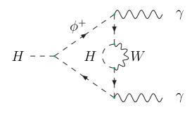
Figure 4: A two-loop diagram containing a quadratically divergent subdiagram (self-energy) associated to the unphysical scalars $\phi$.

The renormalization of the gauge parameter is needed to obtain the finiteness of each of the individual terms in the $q_{4w}$ expansion. In fact, diagrams where the quantum $\phi$ field is exchanged can contain quadratically divergent subdiagrams associated to the $\phi$ self-energy where the Higgs field is present, see Fig. 4. To make these diagrams finite one needs a further subtraction proportional to the derivative of the quantum $\phi$ field self-energy. The counterterm for the gauge parameter that makes each individual term of the Taylor expansion finite is

$$\delta\xi_{Q}=-{\delta m_{\scriptscriptstyle W}^{2}\over m_{\scriptscriptstyle W}^{2}}+\delta Z_{\phi}\,,$$ (17)

where $\delta Z_{\phi}$ is the derivative of the $\phi$ self-energy evaluated at zero momentum transfer. Few observations are now in order. i) As always only the divergent part of $\delta\xi_{Q}$ is fixed. Our choice in Eq. (17) specifies the finite term. As said before, S-matrix elements are insensitive to the renormalization of the gauge parameter and therefore to the prescription used for it. However, in our actual calculation the expansion in $q_{4w}$ includes some higher order terms in $h_{4w}$ and therefore our result contains a residual dependence on the prescription for $\delta\xi_{Q}$. ii) We notice that the first term in the r.h.s. of Eq. (17) has the effect to cancel the Feynman gauge mass renormalization for the $c$ and $\phi$ we have previously introduced, or

$$\left.\delta m^{2}_{c}=\delta(\xi_{Q}m_{\scriptscriptstyle W}^{2})\right|_{\xi_{Q}=1}=\left.m_{\scriptscriptstyle W}^{2}\,\delta\xi_{Q}+\xi_{Q}\,\delta m_{\scriptscriptstyle W}^{2}\right|_{\xi_{Q}=1}=\delta Z_{\phi}m_{\scriptscriptstyle W}^{2}~{}.$$ (18)

Similarly, the $W$ boson propagator is renormalized, a part longitudinal terms proportional to $\delta Z_{\phi}$, as if we were employing in the one-loop part the Landau gauge expression for it.

3 Numerical Results

In this section we present the result of our computation. As explained in the previous section the evaluation of the 1PI contributions ${\cal F}^{2l}_{t,{\scriptscriptstyle W}}|_{1PI}$ has been obtained by expanding the two-loop diagrams in terms of the variable $q_{4w}$, or

$${\cal F}^{2l}_{t,{\scriptscriptstyle W}}|_{1PI}=\frac{\alpha}{4\pi s^{2}}\left(c_{0}+c_{1}q_{4w}+c_{2}q_{4w}^{2}+c_{3}q_{4w}^{3}+{\cal O}(q_{4w}^{4})\right)\,.$$ (19)

The coefficients $c_{i},\,(i=0,..,3)$ depend on $m_{\scriptscriptstyle H}$. Their analytic expressions are too long to be reported here, therefore we present them in a numerical form. The $c_{i}$ coefficients for 100 GeV $<m_{\scriptscriptstyle H}<$ 150 GeV are very well described by a linear fit in $h_{4w}$. Choosing $m_{t}=178$ GeV, $m_{\scriptscriptstyle W}=80.4$ GeV and $m_{\scriptscriptstyle Z}=91.18$ GeV, $s^{2}=1-m_{\scriptscriptstyle W}^{2}/m_{\scriptscriptstyle Z}^{2}$, we obtain for the heavy-quark contribution, ${\cal F}^{2l}_{t}|_{1PI}$,

$$c_{0} = -54.4+6.07\,h_{4w}$$

$$c_{1} = -13.3+3.02\,h_{4w}$$

$$c_{2} = -7.00+1.84\,h_{4w}$$

$$c_{3} = -4.35+1.18\,h_{4w}~{},$$

while for the purely bosonic one, ${\cal F}^{2l}_{{\scriptscriptstyle W}}|_{1PI}$, we have

$$c_{0} = 16.3-1.72\,h_{4w}$$

$$c_{1} = 25.7-2.64\,h_{4w}$$

$$c_{2} = 15.5-2.05\,h_{4w}$$

$$c_{3} = 10.2-1.46\,h_{4w}~{}.$$

$m_{h}$	${\cal F}^{2l}_{{\scriptscriptstyle W}}|_{1PI}$		${\cal F}^{2l}_{t}|_{1PI}$
	truncated	Padé	truncated	Padé
100	27.8	27.9	-57.9	-57.9
105	29.3	29.6	-58.3	-58.4
110	31.1	31.5	-58.8	-59.0
115	32.9	33.6	-59.3	-59.6
120	35.0	35.9	-59.9	-60.2
125	37.2	38.5	-60.5	-61.0
130	39.6	41.5	-61.2	-61.9
135	42.2	45.0	-62.0	-62.9
140	45.1	48.9	-62.8	-64.1
145	48.1	53.6	-63.7	-65.5
150	51.4	59.2	-64.7	-67.2

Table 1: Comparison between normal truncated Taylor expansions of ${\cal F}^{2l}_{t,{\scriptscriptstyle W}}|_{1PI}$ and Padé improved values obtained using Eq. (20). Numbers are given in units of $\alpha/(4\pi s^{2})$.

From the above expressions it is clear that the heavy-quark contribution shows a very good convergence for Higgs masses in the intermediate region while the purely bosonic expansion has a slightly worse behaviour. In both cases, however, the series behave better than a geometric series. In order to improve the convergence of our expansion close to the $2m_{\scriptscriptstyle W}$ threshold, i.e., to estimate the impact of the higher order terms, we employ a Padé approximant. This method has been shown to be a very powerful tool to obtain an approximation to an analytic function $f(x)$ which cannot be computed directly, but it is known for small (and/or large) argument. The generic Padé approximant, $P_{[n/m]}(x)$ is the ratio between two polynomials of degree $n$ and $m$, respectively. It is known that best convergence is achieved when the polynomial in the numerator has degree equal to or greater by one than the polynomial in the denominator, so we choose

$$P_{[2/1]}(x)=\frac{a_{0}+a_{1}x+a_{2}x^{2}}{1+b_{1}x}\,.$$ (20)

The coefficients $a_{i}$ and $b_{i}$ are found by matching the Taylor expansion of Eq. (20) to the coefficients $c_{i}$ of the expansion of Eq. (19). This procedure yields the following set of equations:

$$c_{0}=+a_{0}$$

$$c_{1}=-a_{0}b_{1}+a_{1}$$

$$c_{2}=+a_{0}b_{1}^{2}-a_{1}b_{1}+a_{2}$$

$$c_{3}=-a_{0}b_{1}^{3}+a_{1}b_{1}^{2}-a_{2}b_{1}\,,$$

which can be easily solved in terms of $a_{0,1,2}$ and $b_{1}$. Numerical results are shown in Tab. 1, where the fixed order Taylor expansion and the Padé approximants are given for different Higgs masses. As expected the impact of the improvement is larger close to the $2m_{\scriptscriptstyle W}$ threshold entailing a $15\%$ enhancement for the bosonic expansion and only a $4\%$ for the heavy-quark one. Note that the size of these effects is consistent with estimating the error of the results by using the last coefficient in the Taylor expansion.

$m_{h}$	leptons	lq	$3^{\rm rd}$ gen	YM	2-loop	$\delta_{EW}(\%)$
100	-8.04	-10.9	-30.9	13.5	-36.3	-3.44
105	-8.07	-10.6	-31.3	15.5	-34.5	-3.22
110	-8.07	-10.3	-31.7	17.6	-32.4	-2.97
115	-8.04	-9.86	-32.1	20.0	-30.0	-2.70
120	-7.95	-9.29	-32.6	22.5	-27.2	-2.40
125	-7.82	-8.59	-33.1	25.4	-24.1	-2.07
130	-7.62	-7.75	-33.6	28.5	-20.4	-1.71
135	-7.35	-6.73	-34.2	32.0	-16.2	-1.32
140	-6.98	-5.47	-34.7	35.8	-11.3	-0.88
145	-6.48	-3.89	-35.2	40.0	-5.61	-0.42
150	-5.78	-1.78	-35.5	44.1	1.022	0.072

Table 2: Contributions to ${\cal F}$ at two loops, in units of $\alpha/(4\pi s^{2})$, for various Higgs masses. Starting from the second column, the two-loop contributions of the following classes of diagrams are shown, as listed in Eq. (21): sum of three lepton families, light quarks ($u,d,c,s$), third generation quarks, purely bosonic. The sixth column shows the sum of all the 2-loop EW contribution, ${\cal F}^{2l}$. The last column gives the total EW correction to the decay rate as plotted in Fig. 6.

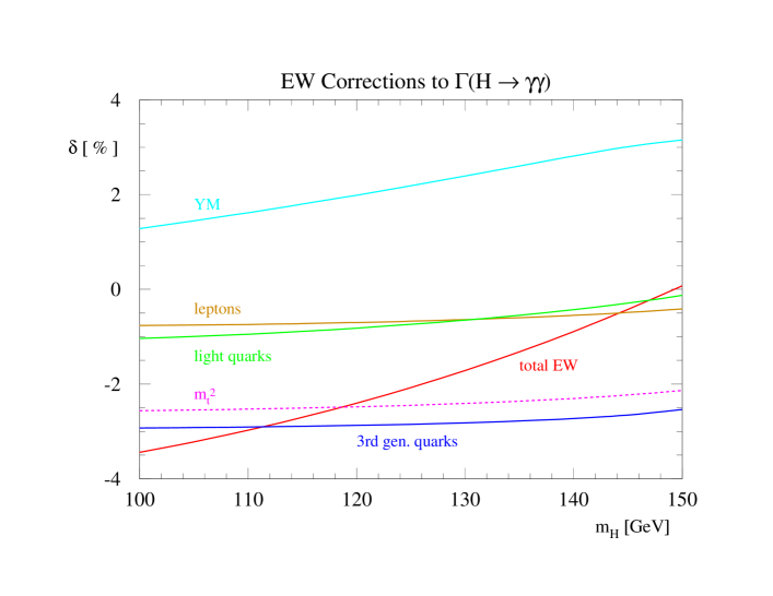
Figure 5: Various contributions to $\delta_{EW}$ as a function of the Higgs mass. Lepton (summed over three families) and light quark contributions ($u,d,c,s$) are the two central curves. Purely bosonic (YM) and third generation quarks are the top and the bottom curves respectively. The large top-mass approximation ($m_{t}^{2}$), which is a subset of the third generation contribution, is also shown (dotted line).

Our result on the heavy corrections can be put together with the result of Ref. [17] on the light fermion contribution to obtain a complete prediction for the two-loop electroweak correction to the decay width,

${\cal F}^{2l}=\frac{\alpha}{4\pi s^{2}}\{$	$+3(w_{\scriptscriptstyle H}C_{W}^{l}A_{2}[0,w_{\scriptscriptstyle H}]+z_{H}C_{Z}^{l}A_{1}[z_{\scriptscriptstyle H}])$	leptons
	$+2(w_{\scriptscriptstyle H}C_{W}^{q}A_{2}[-2/9,w_{\scriptscriptstyle H}]+z_{H}C_{Z}^{q}A_{1}[z_{\scriptscriptstyle H}])$	light quarks
	$+z_{\scriptscriptstyle H}C_{Z}^{b}A_{1}[z_{\scriptscriptstyle H}]+{\cal F}^{2l}_{t}$	third generation quarks
	$+{\cal F}^{2l}_{\scriptscriptstyle W}\left\}\right.$	YM ,

  (21)

where $A_{1}[x]$ and $A_{2}[q,x]$ are defined in Ref. [17], $z_{\scriptscriptstyle H}\equiv m_{\scriptscriptstyle Z}^{2}/m_{\scriptscriptstyle H}^{2}$ and

$$C_{Z}^{q} = \frac{4N_{c}}{c^{2}}\left[Q_{u}^{2}({z_{-}^{u}}^{2}+{z_{+}^{u}}^{2})+Q_{d}^{2}({z_{-}^{d}}^{2}+{z_{+}^{d}}^{2})\right]$$

$$C_{Z}^{l} = \frac{4}{c^{2}}({z_{-}^{l}}^{2}+{z_{+}^{l}}^{2})$$

$$C_{Z}^{b} = \frac{4N_{c}}{c^{2}}Q_{d}^{2}({z_{-}^{d}}^{2}+{z_{+}^{d}}^{2})$$ (22)

$$C_{W}^{q} = 2N_{c}$$

$$C_{W}^{l} = 2\,,$$

with $z_{+}^{i}=T_{3}-Q_{i}s^{2}$ and $z_{-}^{i}=-Q_{i}s^{2}$.

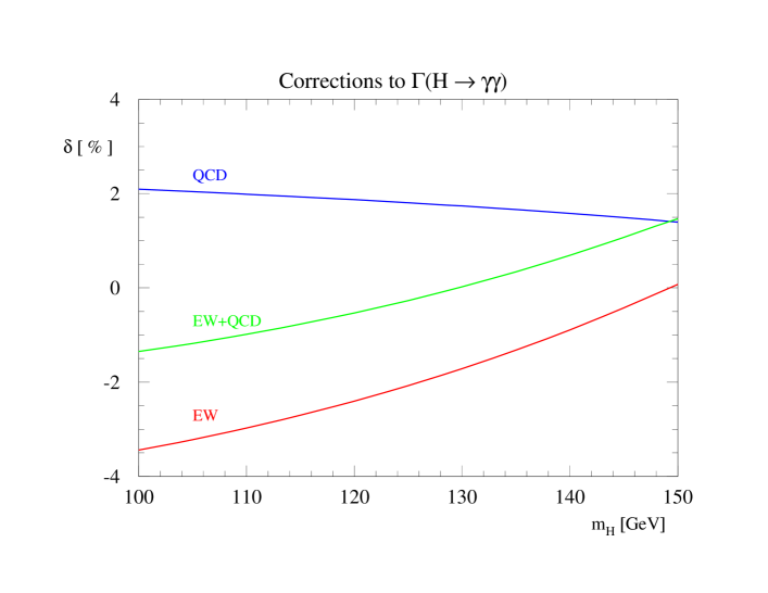
Figure 6: Corrections to the decay rate of $\Gamma(H\to\gamma\gamma)$ for various Higgs masses. The upper curve corresponds to the QCD corrections, the lower curve represents the complete electroweak corrections. Their sum is given by the intermediate curve.

The numerical impact of each of the contributions in Eq. (21) is shown in Tab. 2 . As a generic feature we note that the two-loop contributions involving fermions in the loop are negative, while purely bosonic contributions are positive, in analogy to the one-loop calculation. For Higgs masses around 100 GeV the dominant effect comes from the third generation quarks, with the purely bosonic canceling most of the lepton and light quarks contributions. For higher values of the Higgs mass, the purely bosonic term increases and becomes comparable to the top contribution but with opposite sign. In this region a strong cancellation between the two leading terms takes place, leaving a very small correction as a final result. The corresponding corrections to the width $\Gamma(H\to\gamma\gamma)=\Gamma_{0}\cdot(1+\delta_{EW})$ can be calculated as

$$\delta_{EW}=\frac{2{\rm Re}({\cal F}^{1l}{\cal F}^{2l})}{|{\cal F}^{1l}|^{2}}\,,$$ (23)

and are shown in Fig. 5.

From our expansions it is easy to extract the leading term in $G_{\mu}m_{t}^{2}$, which was calculated in Refs. [15]. We find

$$\lim_{m_{t}\to\infty}{\cal F}^{2l}_{t}=-\frac{\alpha}{4\pi s^{2}}N_{c}Q_{t}^{2}\frac{m_{t}^{2}}{m_{\scriptscriptstyle W}^{2}}\left(\frac{367}{96}+\frac{11}{16}h_{4w}+\frac{19}{56}h_{4w}^{2}+\frac{29}{140}h_{4w}^{3}+{\cal O}(h_{4w}^{4})\right)\,.$$ (24)

The contribution from this (gauge invariant) class of electroweak corrections is also shown in Fig. 5. The first important observation is that indeed the leading term in $G_{\mu}m_{t}^{2}$ approximates quite well the contribution from the third generation quarks in the whole range of Higgs masses between 100 GeV and 150 GeV. However, as shown in Fig. 5, this contribution is never the dominant one. The fact that it approximately reproduces the total electroweak corrections for Higgs masses around 120 GeV is due to a fortuitous cancellation between the purely bosonic and the light quark and lepton terms. In fact, for Higgs masses above 140 GeV, the $G_{\mu}m_{t}^{2}$ contribution is mostly canceled by the purely bosonic one and therefore it is much larger than the total electroweak correction.

Finally, it is interesting to compare and combine the total electroweak correction with the QCD one. As a check of our techniques we have recomputed it as an expansion in terms of $h_{4t}$, obtaining

$${\cal F}^{2l}_{QCD}=\frac{\alpha_{S}}{\pi}\frac{4Q_{t}^{2}N_{c}}{3}\left(1-\frac{122}{135}h_{4t}-\frac{8864}{14175}h_{4t}^{2}-\frac{209186}{496125}h_{4t}^{3}+{\cal O}(h_{4t}^{4})\right)\,,$$ (25)

in complete agreement with the known results [13]. We use the above expansion in our numerical analysis, since it converges very rapidly for Higgs masses in the range we are interested in. The impact of the QCD corrections, shown in Fig. 6, is small and amounts to an increase of about 2% of the decay width. Such a small contribution is expected since for intermediate Higgs masses, the one-loop result is dominated by the bosonic loop, which is unaffected by QCD effects. Due the difference in sign between the EW and QCD contributions, the total correction $\delta_{EW+QCD}$ turns out to be very small, ranging between $-1.5\%$ for $m_{H}=100$ GeV to $1.5\%$ for $m_{H}=150$ GeV and reaching an almost perfect cancellation around $m_{\scriptscriptstyle H}=130$ GeV.

4 Conclusions

We have computed the two-loop electroweak corrections to the decay width of the Higgs into two photons induced by the weak bosons and third generation quarks. By combining our results with those of Ref. [17], involving light fermions in the loops, we have found that the total electroweak corrections to the decay rate are moderate and negative. For Higgs masses between 100 GeV $\lesssim m_{\scriptscriptstyle H}\lesssim$ 150 GeV they range $-4\%\lesssim\delta_{EW}\lesssim 0\%$. Once QCD corrections, which are also small but positive, are added, one finds that $|\delta_{EW+QCD}|$ is always less than $1.5\%$. This shows that the perturbative expansions in $\alpha_{S}$ and $\alpha_{EW}$ for the decay rate are extremely well behaved and a next-to-leading calculation already gives a very reliable prediction. If a similar precision could be matched experimentally, one would have an interesting and powerful test of the standard model.

5 Acknowledgments

We are grateful to Alessandro Vicini for useful discussions.

References

- [1] [LEP Collaboration], arXiv:hep-ex/0412015.
-
[2]
B. C. Allanach, A. Djouadi, J. L. Kneur, W. Porod and P. Slavich,
arXiv:hep-ph/0406166;
G. Degrassi, S. Heinemeyer, W. Hollik, P. Slavich and G. Weiglein, Eur. Phys. J. C 28 (2003) 133 [arXiv:hep-ph/0212020]. - [3] H. M. Georgi, S. L. Glashow, M. E. Machacek and D. V. Nanopoulos, Phys. Rev. Lett. 40 (1978) 692.
- [4] D. L. Rainwater and D. Zeppenfeld, JHEP 9712 (1997) 005 [arXiv:hep-ph/9712271].
- [5] M. Duhrssen, S. Heinemeyer, H. Logan, D. Rainwater, G. Weiglein and D. Zeppenfeld, Phys. Rev. D 70 (2004) 113009 [arXiv:hep-ph/0406323].
- [6] G. Jikia and S. Soldner-Rembold, Nucl. Phys. Proc. Suppl. 82 (2000) 373 [arXiv:hep-ph/9910366].
- [7] D. M. Asner, J. B. Gronberg and J. F. Gunion, Phys. Rev. D 67 (2003) 035009 [arXiv:hep-ph/0110320].
- [8] P. Niezurawski, A. F. Zarnecki and M. Krawczyk, arXiv:hep-ph/0307183.
- [9] G. L. Kane, G. D. Kribs, S. P. Martin and J. D. Wells, Phys. Rev. D 53, 213 (1996) [arXiv:hep-ph/9508265].
- [10] A. Djouadi, V. Driesen, W. Hollik and J. I. Illana, Eur. Phys. J. C 1 (1998) 149 [arXiv:hep-ph/9612362].
- [11] T. Han, H. E. Logan, B. McElrath and L. T. Wang, Phys. Lett. B 563, 191 (2003) [Erratum-ibid. B 603, 257 (2004)] [arXiv:hep-ph/0302188].
-
[12]
J. R. Ellis, M. K. Gaillard and D. V. Nanopoulos,
Nucl. Phys. B 106 (1976) 292;
M. A. Shifman, A. I. Vainshtein, M. B. Voloshin and V. I. Zakharov, Sov. J. Nucl. Phys. 30 (1979) 711 [Yad. Fiz. 30 (1979) 1368]. -
[13]
H. . Zheng and D. . Wu,
Phys. Rev. D 42 (1990) 3760;
A. Djouadi, M. Spira, J. J. van der Bij and P. M. Zerwas, Phys. Lett. B 257, 187 (1991);
S. Dawson and R. P. Kauffman, Phys. Rev. D 47 (1993) 1264;
A. Djouadi, M. Spira and P. M. Zerwas, Phys. Lett. B 311 (1993) 255 [arXiv:hep-ph/9305335];
K. Melnikov and O. I. Yakovlev, Phys. Lett. B 312 (1993) 179 [arXiv:hep-ph/9302281];
M. Inoue, R. Najima, T. Oka and J. Saito, Mod. Phys. Lett. A 9 (1994) 1189;
M. Steinhauser, arXiv:hep-ph/9612395;
J. Fleischer, O. V. Tarasov and V. O. Tarasov, Phys. Lett. B 584 (2004) 294 [arXiv:hep-ph/0401090]. -
[14]
Y. Liao and X. y. Li,
Phys. Lett. B 396 (1997) 225
[arXiv:hep-ph/9605310];
A. Djouadi, P. Gambino and B. A. Kniehl, Nucl. Phys. B 523 (1998) 17 [arXiv:hep-ph/9712330]. - [15] F. Fugel, B. A. Kniehl and M. Steinhauser, Nucl. Phys. B 702 (2004) 333 [arXiv:hep-ph/0405232].
- [16] J. G. Korner, K. Melnikov and O. I. Yakovlev, Phys. Rev. D 53 (1996) 3737 [arXiv:hep-ph/9508334].
-
[17]
U. Aglietti, R. Bonciani, G. Degrassi and A. Vicini,
Phys. Lett. B 595 (2004) 432
[arXiv:hep-ph/0404071];
U. Aglietti, R. Bonciani, G. Degrassi and A. Vicini, Phys. Lett. B 600 (2004) 57 [arXiv:hep-ph/0407162]. -
[18]
E. Remiddi and J. A. M. Vermaseren,
Int. J. Mod. Phys. A 15 (2000) 725
[arXiv:hep-ph/9905237];
T. Gehrmann and E. Remiddi, Comput. Phys. Commun. 144 (2002) 200 [arXiv:hep-ph/0111255]. - [19] U. Aglietti and R. Bonciani, Nucl. Phys. B 698 (2004) 277 [arXiv:hep-ph/0401193].
- [20] G. Degrassi and F. Maltoni, Phys. Lett. B 600 (2004) 255 [arXiv:hep-ph/0407249].
-
[21]
B. S. Dewitt,
Phys. Rev. 162 (1967) 1195 ;
J. Honerkamp, Nucl. Phys. B 48 (1972) 269 ;
H. Kluberg-Stern and J. B. Zuber, Phys. Rev. D 12 (1975) 482. - [22] L. F. Abbott, Nucl. Phys. B 185 (1981) 189.
- [23] A. Denner, G. Weiglein and S. Dittmaier, Nucl. Phys. B 440 (1995) 95 [arXiv:hep-ph/9410338].
- [24] D. Binosi and J. Papavassiliou, Phys. Rev. D 66 (2002) 076010 [arXiv:hep-ph/0204308].
-
[25]
J.M. Cornwall, in Proceedings of the French–American
Seminar on Theoretical Aspects of Quantum Chromodynamics,
Marseille, France, 1981, edited by J.W. Dash (Centre de
Physique Theorique Reports No. CPT–81/P–1345, Marseille, 1982);
J. M. Cornwall, Phys. Rev. D 26 (1982) 1453;
J. M. Cornwall and J. Papavassiliou, Phys. Rev. D 40 (1989) 3474;
J. Papavassiliou, Phys. Rev. D 41 (1990) 3179;
G. Degrassi and A. Sirlin, Phys. Rev. D 46 (1992) 3104. -
[26]
B. A. Kniehl, C. P. Palisoc and A. Sirlin,
Nucl. Phys. B 591 (2000) 296
[arXiv:hep-ph/0007002];
J. Papavassiliou and A. Pilaftsis, Phys. Rev. D 58 (1998) 053002 [arXiv:hep-ph/9710426]. - [27] T. Hahn, Comput. Phys. Commun. 140 (2001) 418 [arXiv:hep-ph/0012260].
- [28] O. V. Tarasov, arXiv:hep-ph/9505277.
- [29] A. I. Davydychev and J. B. Tausk, Nucl. Phys. B 397, 123 (1993).
- [30] A. Sirlin and R. Zucchini, Nucl. Phys. B 266 (1986) 389.
- [31] R. V. Harlander, in Proc. of the 5th International Symposium on Radiative Corrections (RADCOR 2000) ed. Howard E. Haber, arXiv:hep-ph/0102266.