How Magnetic is the Dirac Neutrino?

Abstract

We derive model-independent, “naturalness” upper bounds on the magnetic moments $\mu_{\nu}$ of Dirac neutrinos generated by physics above the scale of electroweak symmetry breaking. In the absence of fine-tuning of effective operator coefficients, we find that current information on neutrino mass implies that $|\mu_{\nu}|~{}{}_{\textstyle\sim}^{\textstyle<}~{}10^{-14}$ Bohr magnetons. This bound is several orders of magnitude stronger than those obtained from analyses of solar and reactor neutrino data and astrophysical observations.

With the current emphasis on understanding the pattern of neutrino mass and mixing and the corresponding implications for cosmology and astrophysics, it is also of interest to consider the electromagnetic properties of the neutrino. The leading coupling of the neutrino to the photon is the magnetic moment, $\mu_{\nu}$. The chiral symmetry obeyed by the massless neutrinos of the Standard Model (SM) requires that $\mu_{\nu}=0$. Now that we know that $m_{\nu}\not=0$, however, it is interesting to ask how large one might expect the neutrino magnetic moment to be. In the minimally extended SM containing gauge-singlet right-handed neutrinos, one finds that $\mu_{\nu}$ is non-vanishing, but unobservably small: $\mu_{\nu}\approx 3\times 10^{-19}\mu_{B}[m_{\nu}/1\ {\rm eV}]$ Marciano:1977wx .

Current experimental limits are several orders of magnitude larger. Those obtained from laboratory experiments are based on analyses of the recoiling electron kinetic energy $T$ in neutrino-electron scattering. The effect of a non-vanishing $\mu_{\nu}$ will be recognizable only if the corresponding electromagnetic cross section is comparable in magnitude with the well-understood weak interaction cross section. The magnitude of $\mu_{\nu}$ which can be probed in this way is then given by

$$\frac{|\mu_{\nu}^{\rm exp}|}{\mu_{B}}\simeq\frac{G_{F}\,m_{e}}{\sqrt{2}\pi\alpha}\sqrt{m_{e}T}\sim 10^{-10}\sqrt{\frac{T}{m_{e}}}\ \ .$$ (1)

Considering realistic values of $T$, it would be difficult to reach sensitivities below $\sim 10^{-11}\mu_{B}$. The limits derived from studies of solar and reactor neutrinos are presently somewhat weaker: $|\mu_{\nu}|~{}{}_{\textstyle\sim}^{\textstyle<}~{}1.5\times 10^{-10}\mu_{B}$ (solar) beacom and $|\mu_{\nu}|~{}{}_{\textstyle\sim}^{\textstyle<}~{}0.9\times 10^{-10}\mu_{B}$ (reactor), MUNU .

Limits on $\mu_{\nu}$ can also be derived from bounds on unobserved energy loss in astrophysical objects. For sufficiently large $\mu_{\nu}$, the rate for plasmon decay into $\nu{\bar{\nu}}$ pairs would conflict with such bounds. Since plasmons can also decay weakly into $\nu{\bar{\nu}}$ pairs, the sensitivity of this probe is again limited by size of the weak rate, leading to Sutherland:1975dr

$$\frac{|\mu_{\nu}^{\rm astro}|}{\mu_{B}}\simeq\frac{G_{F}\,m_{e}}{\sqrt{2}\pi\alpha}\left(\hbar\omega_{P}\right)\ \ ,$$ (2)

where $\omega_{P}$ is the plasma frequency. Since $(\hbar\omega_{P})^{2}\ll m_{e}T$, this bound is stronger than the limit in Eq. (1). Given the appropriate values of $\hbar\omega_{P}$ it would be difficult to reach sensitivities better than $10^{-12}\mu_{B}$. Indeed, from the analysis performed in Ref. raffelt , one obtains $|\mu_{\nu}|~{}{}_{\textstyle\sim}^{\textstyle<}~{}3\times 10^{-12}\mu_{B}$.

In what follows, we show – in a general and model-independent way – that a magnetic moment of a Dirac neutrino with magnitude of the same order, or just below, current limits would be unnaturally large and would require the existence of fine tuning in order to prevent unacceptably large contributions to $m_{\nu}$ via radiative corrections. Although small Dirac neutrino masses imply very small Yukawa couplings, they are not inconsistent with observations. In order to satisfy $m_{\nu}\lesssim 1{\rm eV}$, we argue that a more natural scale for $|\mu_{\nu}|$ would be $~{}{}_{\textstyle\sim}^{\textstyle<}~{}10^{-14}\mu_{B}$.

Assuming that $\mu_{\nu}$ is generated by some physics beyond the SM at a scale $\Lambda$, its leading contribution to the neutrino mass, $\delta m_{\nu}$, scales with $\Lambda$ as

$$\delta m_{\nu}\sim\frac{\alpha}{32\pi}\frac{\Lambda^{2}}{m_{e}}\frac{\mu_{\nu}}{\mu_{B}}\ \ ,$$ (3)

where, $\delta m_{\nu}$ is the contribution to a generic entry in the $3\times 3$ neutrino mass matrix arising from radiative corrections at one-loop order. The dependence on $\Lambda^{2}$ arises from the quadratic divergence appearing in the renormalization of the dimension four neutrino mass operator. Although the precise value of the coefficient on the right side of Eq. (3) can only be obtained with the use of a specific model, it implies an order-of-magnitude bound on the size of $\mu_{\nu}$. For $\Lambda\sim 1$ TeV, requiring that $\delta m_{\nu}$ not be significantly larger than one eV implies that $|\mu_{\nu}|~{}{}_{\textstyle\sim}^{\textstyle<}~{}10^{-14}\mu_{B}$. Given the quadratic dependence on $\Lambda$, this bound becomes considerably more stringent as the scale of new physics is increased from the scale of electroweak symmetry breaking, $v\sim 250$ GeV.

The problem of reconciling a large magnetic moment with a small mass has been recognized in the past, and the quadratic dependence on $\Lambda$ in Eq. (3) discussed in, e.g., Barr ; Voloshin . Possible ways of overcoming this restriction include imposing a symmetry to enforce $m_{\nu}=0$ while allowing a non-zero value for $\mu_{\nu}$ Voloshin , or employing a spin suppression mechanism to keep $m_{\nu}$ small Barr . Neutrino magnetic moments are reviewed in Fukugita ; boris ; Wong , and recent work can be found in McLaughlin .

When $\Lambda$ is not substantially larger than $v$, the contribution to $\delta m_{\nu}$ from higher dimension operators can be important, and their renormalization due to operators responsible for the neutrino magnetic moment can be computed in a model-independent way. As we discuss below, dimension six operators are the lowest that contribute. We shall now outline this calculation and the resulting constraints on $\mu_{\nu}$. Specifically, we find that

$$\frac{|\mu_{\nu}|}{\mu_{B}}=\frac{G_{F}\,m_{e}}{\sqrt{2}\pi\alpha}\ \left[\frac{\delta m_{\nu}}{\alpha\,\ln(\Lambda/v)}\right]\ \frac{32\pi\sin^{4}\theta_{W}}{9\,|f|}\ \ \ ,$$ (4)

where $\theta_{W}$ is the weak mixing angle,

$$f=\left(1-r\right)-\frac{2}{3}r\tan^{2}\theta_{W}-\frac{1}{3}\left(1+r\right)\tan^{4}\theta_{W}\ \ \ ,$$ (5)

and $r=C_{-}/C_{+}$ is a ratio of effective operator coefficients defined at the scale $\Lambda$ (see below) that one expects to be of order unity. Again taking $\Lambda\sim\ 1$ TeV, $\delta m_{\nu}\lesssim 1{\rm eV}$, and setting $r\sim 1$, we find that $\mu_{\nu}$ (for any mass eigenstate) should be smaller in magnitude than $\sim 10^{-14}\mu_{B}$.

To arrive at these conclusions, we consider an effective theory containing Dirac fermions, scalars, and gauge bosons that is valid below the scale $\Lambda$ and that respects the SU(2)${}_{L}\times$ U(1)_Y symmetry of the SM. We also impose lepton number conservation. In this effective theory, the right-handed components of the neutrino have zero hypercharge ($Y$) and weak isospin. The effective Lagrangian involving the $\nu_{R}$, left-handed lepton isodoublet $L$, and Higgs doublet $\phi$ obtained by integrating out physics above the scale $\Lambda$ is given by

$${\cal L}_{\rm eff}=\sum_{n,j}{C^{n}_{j}(\mu)\over\Lambda^{n-4}}\ {\cal O}^{(n)}_{j}(\mu)\ +\ \ {\rm h.c.}\ \,$$ (6)

where the $n\geq 4$ denotes the operator dimension, $j$ runs over all independent operators of a given dimension, and $\mu$ is the renormalization scale. For simplicity, we do not write down the $n=4$ operators appearing in the SM Lagrangian or the Dirac Lagrangian for the $\nu_{R}$. At $n=4$, a neutrino mass would arise from the operator ${\cal O}^{(4)}_{1}={\bar{L}}{\tilde{\phi}}\nu_{R}$, where ${\tilde{\phi}}=i\tau_{2}\phi^{\ast}$. We also omit explicit flavor indices on the $L$ and $\nu_{R}$ fields. After spontaneous symmetry breaking (SSB) at the weak scale,

$$\phi\rightarrow\left(\begin{array}[]{c}0\\ v/\sqrt{2}\end{array}\right)$$ (7)

so that $C^{4}_{1}{\cal O}^{(4)}_{1}\to-m_{\nu}{\bar{\nu}}_{L}\nu_{R}$ with $m_{\nu}=-C^{4}_{1}v/\sqrt{2}$. Consistency with the present information on the scale of $m_{\nu}$ requires that $|C^{4}_{1}|~{}{}_{\textstyle\sim}^{\textstyle<}~{}5\times 10^{-12}$.

A neutrino magnetic moment coupling would be generated by gauge-invariant, dimension six operators that couple the matter fields to the SU(2)_L and U(1)_Y gauge fields $W_{\mu}^{a}$ and $B_{\mu}$, respectively. Above the scale $v$, these operators will mix under renormalization with other $n=6$ operators that contain the $L$, $\nu_{R}$, and $\phi$ and that generate neutrino mass terms after SSB. For this purpose, the basis of independent $n=6$ operators that close under renormalization is given by

$${\cal O}^{(6)}_{1} = g_{1}{\bar{L}}{\tilde{\phi}}\sigma^{\mu\nu}\nu_{R}B_{\mu\nu}$$

$${\cal O}^{(6)}_{2} = g_{2}{\bar{L}}\tau^{a}{\tilde{\phi}}\sigma^{\mu\nu}\nu_{R}W_{\mu\nu}^{a}$$ (8)

$${\cal O}^{(6)}_{3} = {\bar{L}}{\tilde{\phi}}\nu_{R}\left(\phi^{\dagger}\phi\right)\ \ \ ,$$

where $B_{\mu\nu}=\partial_{\mu}B_{\nu}-\partial_{\nu}B_{\mu}$ and $W_{\mu\nu}^{a}=\partial_{\mu}W_{\nu}^{a}-\partial_{\nu}W_{\mu}^{a}-g_{2}\epsilon_{abc}W_{\mu}^{b}W_{\nu}^{c}$ are the U(1)_Y and SU(2)_L field strength tensors, respectively, and $g_{1}$ and $g_{2}$ are the corresponding couplings. After SSB one has

$${\cal O}^{(6)}_{1} \to \frac{v}{\sqrt{2}}g_{1}{\bar{\nu}}_{L}\sigma^{\mu\nu}\nu_{R}B_{\mu\nu}$$ (9)

$${\cal O}^{(6)}_{2} \to g_{2}\frac{v}{\sqrt{2}}{\bar{\nu}}_{L}\sigma^{\mu\nu}\nu_{R}W_{\mu\nu}^{3}+\cdots\ \ \ .$$ (10)

Using $g_{2}\sin\theta_{W}=g_{1}\cos\theta_{W}=e$, it is straightforward to see that the combination $C^{6}_{1}{\cal O}^{(6)}_{1}+C^{6}_{2}{\cal O}^{(6)}_{2}$ appearing in ${\cal L}_{\rm eff}$ contains the magnetic moment operator

$$-{\mu_{\nu}\over 4}{\bar{\nu}}\sigma^{\mu\nu}\nu F_{\mu\nu}$$ (11)

where $F_{\mu\nu}$ is the photon field strength tensor and

$$\frac{\mu_{\nu}}{\mu_{B}}=-4\sqrt{2}\left(\frac{m_{e}v}{\Lambda^{2}}\right)\left[C^{6}_{1}(v)+C^{6}_{2}(v)\right]\ \ \ .$$ (12)

Similarly, the operator ${\cal O}^{(6)}_{3}$ generates a contribution to the neutrino mass

$$\delta m_{\nu}=-C^{6}_{3}(v)\frac{v^{3}}{2\sqrt{2}\Lambda^{2}}\ \ \ .$$ (13)

Other $n=6$ operators that one can write down are either related to those in Eqs. (8) by the equations of motion or do not couple to $F_{\mu\nu}$ after SSB. It is instructive to consider a few illustrative examples. In particular, consider the following three operators:

$${\cal O}^{(6)}_{4} = {\bar{L}}{\overleftarrow{D}}_{\mu}^{\dagger}{\overleftarrow{D}}^{\mu\ {\dagger}}{\tilde{\phi}}\nu_{R}$$ (14)

$${\cal O}^{(6)}_{5} = {\bar{L}}{\overleftarrow{D}}_{\mu}^{\dagger}{\tilde{\phi}}\partial^{\mu}\nu_{R}$$ (15)

$${\cal O}^{(6)}_{6} = {\bar{L}}\tau^{a}{\tilde{\phi}}\nu_{R}\left(\phi^{\dagger}\tau^{a}\phi\right)\ \ \ ,$$ (16)

where $D_{\mu}=\partial_{\mu}+ig_{2}\tau^{a}W_{\mu}^{a}/2+ig_{1}YB_{\mu}/2$ and where the sum over $a=1,2,3$ in ${\cal O}^{(6)}_{6}$ is implied. We may express ${\cal O}^{(6)}_{4}$ in terms of ${\cal O}^{(6)}_{1,2}$ by first noting that

$$0={\bar{L}}{\overleftarrow{\not\!\!D}}^{\dagger}{\overleftarrow{\not\!\!D}}^{\dagger}{\tilde{\phi}}\nu_{R}$$ (17)

since ${\bar{L}}{\overleftarrow{\not\!\!D}}^{\dagger}=0={\not\!\!D}L$ by the equation of motion for $L$. Then using $\gamma_{\mu}\gamma_{\nu}=g_{\mu\nu}-i\sigma_{\mu\nu}$ we have

$$0={\bar{L}}{\overleftarrow{D}}_{\mu}^{\dagger}{\overleftarrow{D}}^{\mu{\dagger}}{\tilde{\phi}}\nu_{R}-\frac{i}{2}{\bar{L}}[{\overleftarrow{D}}_{\mu}^{\dagger},{\overleftarrow{D}}_{\nu}^{\dagger}]\sigma^{\mu\nu}{\tilde{\phi}}\nu_{R}\ \ \ .$$ (18)

Working out the commutator $[{\overleftarrow{D}}_{\mu}^{\dagger},{\overleftarrow{D}}_{\nu}^{\dagger}]$ in terms of $B_{\mu\nu}$ and $W_{\mu\nu}^{a}$ gives

$${\bar{L}}{\overleftarrow{D}}_{\mu}^{\dagger}{\overleftarrow{D}}^{\mu{\dagger}}{\tilde{\phi}}\nu_{R}=-\frac{1}{4}\left[Y_{L}{\cal O}^{(6)}_{1}+{\cal O}^{(6)}_{2}\right]\ \ \ .$$ (19)

where $Y_{L}=-1$ is the lepton doublet hypercharge.

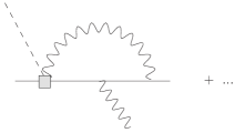
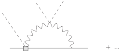
Figure 1: Self-renormalization of ${\cal O}_{1,2}^{(6)}$, denoted by the shaded box. Solid, dashed, and wavy lines indicate leptons, Higgs, and gauge bosons, respectively.

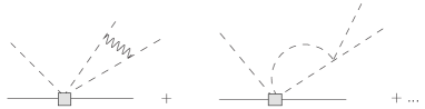
Figure 2: Renormalization of ${\cal O}^{(6)}_{3}$ due to insertions of ${\cal O}_{1,2}^{(6)}$.

Figure 3: Self-renormalization of ${\cal O}_{3}^{(6)}$.

In the case of ${\cal O}^{(6)}_{5}$, the component involving ${\bar{\nu}}_{L}{\overleftarrow{D}}_{\mu}^{\dagger}\phi^{0\ast}\partial^{\mu}\nu_{R}$ contains only the combination $g_{2}W_{\mu}^{3}-g_{1}B_{\mu}\propto Z_{\mu}$ since the SM Lagrangian for the neutrino contains no coupling to the photon. Moreover, since ${\cal O}^{(6)}_{5}$ contains a derivative acting on $\nu_{R}$ and $\nu_{R}$ has no gauge interactions, it does not mix with ${\cal O}^{(6)}_{1-3}$ under renormalization. Finally, one can show that ${\cal O}^{(6)}_{6}=-{\cal O}^{(6)}_{3}$ using the identity $\tau^{a}_{ij}\tau^{a}_{kl}=2\delta_{il}\delta_{jk}-\delta_{ij}\delta_{kl}$. Other operators that contain derivatives acting on the $\phi$ may be related to ${\cal O}^{(6)}_{1,2}$ using integration by parts and the foregoing arguments.

The one-loop renormalization of the ${\cal O}^{(6)}_{1-3}$ is obtained by computing Feynman diagrams of Figs. 1-3, where only representative examples of the full set of graphs are shown. The graphs of Fig. 3 involve renormalization of ${\cal O}^{(6)}_{1,2}$, where the shaded box indicates insertions of the tree-level operator. Graphs of the type shown in Fig. 3 give renormalization of ${\cal O}^{(6)}_{3}$ by insertions of the ${\cal O}^{(6)}_{1,2}$. At this order, there are no insertions of ${\cal O}^{(6)}_{3}$ that renormalize the ${\cal O}^{(6)}_{1,2}$. Graphs leading to self-renormalization of ${\cal O}^{(6)}_{3}$ generated by gauge and $\lambda(\phi^{\dagger}\phi)^{2}$ couplings are illustrated in Fig. 3. For the diagrams involving internal gauge boson lines, we use the background field gaugeAbbott:1980hw , which allows us to obtain gauge-invariant results in a straightforward manner. Throughout, we use dimensional regularization, working in $d=4-2\epsilon$ dimensions, and introduce the renormalization scale $\mu$. Due to operator mixing, the renormalized operators ${\cal O}^{(6)}_{jR}$ can be expressed in terms of the un-renormalized operators ${\cal O}^{(6)}_{j}$ via

$${\cal O}^{(6)}_{jR}=\sum_{k}Z^{-1}_{jk}Z_{L}^{1/2}Z_{\phi}^{n_{\phi}/2}{\cal O}^{(6)}_{k}\ \ \ ,$$ (20)

where $Z_{L}^{1/2}$ and $Z_{\phi}^{1/2}$ are wavefunction renormalization constants for the $L$ and $\phi$ respectively and where $n_{\phi}=1$ (3) is the number of $\phi$ fields appearing in ${\cal O}^{(6)}_{1,2}$ (${\cal O}^{(6)}_{3}$). In the minimal subtraction scheme that we adopt here, the products of renormalization constants $Z^{-1}_{jk}Z_{L}^{1/2}Z_{\phi}^{n_{\phi}/2}$ simply remove the $1/\epsilon$ terms arising from the loop graphs.

The renormalized operators ${\cal O}^{(6)}_{jR}$ are dependent on the scale $\mu$ since the bare operators

$${\cal O}^{(6)}_{j0}=Z_{L}^{1/2}Z_{\phi}^{n_{\phi}/2}{\cal O}^{(6)}_{j}=\sum_{k}Z_{jk}{\cal O}^{(6)}_{kR}$$ (21)

must be $\mu$-independent. The $\mu$-dependence of the $C_{i}^{6}(\mu)$ is such that the renormalized effective Lagrangian ${\cal L}_{\rm eff}^{R}$ does not depend on the renormalization scale. In order to obtain Eq. (4) we require the value of the $C^{6}_{i}(\mu)$ at the scale $\mu=v$, below which the $Z$ and $W^{\pm}$ are integrated out of the effective theory and only the photon contributes to operator renormalization. Since $Q_{\nu}=0$, the latter occurs at higher order in $\alpha/4\pi$ than considered here. The value of the $C^{6}_{i}(v)$ are determined by the renormalization group equation (RGE) that follows from the requirement that ${\cal L}_{\rm eff}^{R}$ be $\mu$-independent:

$$\mu\frac{d}{d\mu}{\cal L}_{\rm eff}^{R}=0\ \Rightarrow\ \mu\frac{d}{d\mu}C^{6}_{j}+\sum_{k}C^{6}_{k}\ \gamma_{kj}=0\ \ \ ,$$ (22)

where the anomalous dimension matrix is defined by

$$\gamma_{kj}=\sum_{\ell}\left(\mu\frac{d}{d\mu}Z_{k\ell}^{-1}\right)Z_{\ell j}\ \ \ .$$ (23)

We find

$$\gamma_{jk}=\left(\begin{array}[]{ccc}-\frac{3}{16\pi}(\alpha_{1}-3\alpha_{2})&\frac{3}{8\pi}\alpha_{1}&-6\alpha_{1}(\alpha_{1}+\alpha_{2})\\ \frac{9}{8\pi}\alpha_{2}&\frac{3}{16\pi}(\alpha_{1}-3\alpha_{2})&6\alpha_{2}(\alpha_{1}+3\alpha_{2})\\ 0&0&\frac{9}{16\pi}(\alpha_{1}+3\alpha_{2})-\frac{5}{4\pi^{2}}\lambda\end{array}\right)\ \ \ ,$$ (24)

where the $\alpha_{i}=g_{i}^{2}/4\pi$ and $V(\phi)=\lambda[(\phi^{\dagger}\phi)-v^{2}/2]^{2}$.

Using the known $\beta$-functions that govern the $\mu$-dependence of the $g_{i}$ and the anomalous dimension matrix in Eq. (24) we numerically solve the RGE (22) for the $C^{6}_{i}(\mu)$. In doing so, we find that the $\mu$-dependence of the $g_{i}$ has a negligible impact on the overall solution. Neglecting the $\mu$-dependence of the $g_{i}$ then allows us to obtain an analytic solution. In this approximation we find that the combinations of constants $C_{+}(\mu)\equiv C_{1}^{6}(\mu)+C_{2}^{6}(\mu)$ and $\tilde{C}(\mu)\equiv\alpha_{1}C_{1}^{6}(\mu)-3\alpha_{2}C_{2}^{6}(\mu)$ evolve independently. Since $\mu_{\nu}$ is proportional to $C_{+}(v)$, the presence of a non-zero neutrino magnetic moment at low energy requires the physics beyond the SM to have generated a non-vanishing $C_{+}(\Lambda)$. It is then straightforward to obtain $C_{3}^{6}(\mu)$ which depends on all three of the $C_{i}^{6}(\Lambda)$. Retaining only the leading logarithms rather than the full resummation provided by the RGE and defining $C_{-}(\mu)=C^{6}_{1}(\mu)-C^{6}_{2}(\mu)$ we find

$$C_{+}(\mu) = C_{+}(\Lambda)\left[1-{\tilde{\gamma}}\ln\frac{\mu}{\Lambda}\right]$$ (25)

$$\tilde{C}(\mu) = \tilde{C}(\Lambda)\left[1+{\tilde{\gamma}}\ln\frac{\mu}{\Lambda}\right]$$

$$C^{6}_{3}(\mu) = C^{6}_{3}(\Lambda)\left[1-\gamma_{33}\ln\frac{\mu}{\Lambda}\right]$$

$$- \left[C_{+}(\Lambda)\gamma_{+}+C_{-}(\Lambda)\gamma_{-}\right]\ln\frac{\mu}{\Lambda}\ \ \ ,$$

where $\gamma_{\pm}=(\gamma_{13}\pm\gamma_{23})/2$ and ${\tilde{\gamma}}=3(\alpha_{1}+3\alpha_{2})/16\pi$.

Using Eqs. (12,13) allows us to relate $\mu_{\nu}$ to the corresponding neutrino mass matrix element in terms of $C_{\pm}(\Lambda)$ and $C^{6}_{3}(\Lambda)$

$$\delta m_{\nu}=\frac{v^{2}}{16m_{e}}\ \frac{C^{6}_{3}(v)}{C_{+}(v)}\ \frac{\mu_{\nu}}{\mu_{B}}\ \ \ \ ,$$ (26)

with $C_{+}(v)$ and $C^{6}_{3}(v)$ given approximately by Eqs. (25). To obtain a natural upper bound on $\mu_{\nu}$, we assume first that $C^{6}_{3}(\Lambda)=0$ so that $\delta m_{\nu}$ is generated entirely by radiative corrections involving insertions of ${\cal O}^{(6)}_{1,2}$. Doing so in Eq. (26) and solving for $\mu_{\nu}/\mu_{B}$ leads directly to Eq. (4). To arrive at a numerical estimate of this bound, we substitute $\Lambda=1$ TeV into the logarithms appearing in Eq. (4) and obtain

$$\frac{|\mu_{\nu}|}{\mu_{B}}~{}{}_{\textstyle\sim}^{\textstyle<}~{}8\times 10^{-15}\times\left(\frac{\delta m_{\nu}}{1\ {\rm eV}}\right)\frac{1}{|f|}\ \ \ .$$ (27)

It is interesting to consider the bound for the special case that only the magnetic moment operator is generated at the scale $\Lambda$, i.e., $C_{+}(\Lambda)\not=0$ and $C_{-}=0$, with $f\simeq 1$. For this case, considering a nearly degenerate neutrino spectrum with masses $\sim 1$ eV leads to the $|\mu_{\nu}|~{}{}_{\textstyle\sim}^{\textstyle<}~{}8\times 10^{-15}\mu_{B}$ – a limit that is two orders of magnitude stronger than the astrophysical bound raffelt and $10^{4}$ stronger than those obtained from solar and reactor neutrinos. For a hierarchical neutrino mass spectrum, the bound would be even more stringent.

The discovery of a Dirac neutrino magnetic moment having a magnitude comparable to, or just below, the present experimental limits would imply considerable fine-tuning in order to maintain consistency with the scale of neutrino mass. Such fine-tuning could occur through cancellations between the $C_{+}(\Lambda)$, $C_{-}(\Lambda)$, and $C^{6}_{3}(\Lambda)$ terms in Eq. (25). While it is in principle possible to construct a model that displays such fine-tuning, the generic situation implies substantially smaller magnetic moments for Dirac neutrinos than are presently accessible through observation.

The limits one may obtain on transition magnetic moments of Majorana neutrinos are substantially weaker than those for the Dirac moment. Because the transition magnetic moment $\mu_{\nu}^{ij}$ is antisymmetric in the flavor labels $i$, $j$, while the mass matrix is symmetric, $\delta m_{\nu}$ must be higher order in $\mu_{\nu}^{ij}$ or involve insertions of the Yukawa couplings.

References

(1)
W. J. Marciano and A. I. Sanda,
Phys. Lett. B 67, 303 (1977);
B. W. Lee and R. E. Shrock,
Phys. Rev. D 16, 1444 (1977);
K. Fujikawa and R. Shrock,
Phys. Rev. Lett. 45, 963 (1980).
(2)
J. F. Beacom and P. Vogel,
Phys. Rev. Lett. 83, 5222 (1999);
D. W. Liu et al.,
Phys. Rev. Lett. 93, 021802 (2004).
(3)
Z. Daraktchieva et al. [MUNU Collaboration],
Phys. Lett. B 615, 153 (2005);
B. Xin et al. [TEXONO Collaboration],
Phys. Rev. D 72, 012006 (2005).
(4)
P. Sutherland, J. N. Ng, E. Flowers, M. Ruderman and C. Inman,
Phys. Rev. D 13, 2700 (1976).
(5) G.G. Raffelt, Phys. Rep. 320, 319 (1999).
(6)
J. Schechter and J. W. F. Valle,
Phys. Rev. D 25, 2951 (1982).
(7)
T. M. Ito and G. Prezeau,
Phys. Rev. Lett. 94, 161802 (2005);
G. Prezeau and A. Kurylov,
hep-ph/0409193.
(8)
M. B. Voloshin,
Sov. J. Nucl. Phys. 48, 512 (1988)
(9)
S. M. Barr, E. M. Freire and A. Zee,
Phys. Rev. Lett. 65, 2626 (1990).
(10)
L. F. Abbott,
Nucl. Phys. B 185, 189 (1981).
(11)
M. Fukugita and T. Yanagida,
Physics of neutrinos and applications to astrophysics,
Chapter 10, Springer, Berlin, (2003), and references therein.
(12)
B. Kayser, F. Gibrat-Debu and F. Perrier,
World Sci. Lect. Notes Phys. 25, 1 (1989).
(13)
H. T. Wong and H. B. Li,
Mod. Phys. Lett. A 20, 1103 (2005).
(14)
G. C. McLaughlin and J. N. Ng,
Phys. Lett. B 470, 157 (1999);
R. N. Mohapatra, S. P. Ng and H. b. Yu,
Phys. Rev. D 70, 057301 (2004).