We discuss a possible new resonance in active-sterile neutrino oscillations arising in theories with large extra dimensions. Fluctuations in the brane effectively increase the path-length of active neutrinos relative to the path-length of sterile neutrinos through the extra-dimensional bulk. Well below the resonance, the standard oscillation formulas apply. Well above the resonance, active-sterile oscillations are suppressed. We show that a resonance energy in the range of $30-400$ MeV allows an explanation of all neutrino oscillation data, including LSND data, in a consistent four-neutrino model. A high resonance energy implies an enhanced signal in MiniBooNE. A low resonance energy implies a distorted energy spectrum in LSND, and an enhanced $\nu_{\mu}$ depletion from a stopped-pion source. The numerical value of the resonance energy may be related back to the geometric aspects of the brane world. Some astrophysical and cosmological consequences of the brane-bulk resonance are briefly sketched.

1 Introduction

Theories with large extra dimensions typically confine the Standard Model (SM) particles on a 3+1 brane embedded in an extra-dimensional bulk [1, 2] see also [3]. Gauge singlet particles may travel on or off the brane. These include the graviton, and any singlet ($\equiv$ “sterile”) neutrinos [4]. Virtual gravitons, too, penetrate the bulk, and so lead via Gauss’ Law to an apparent weak gravity on our brane, when in fact the strength of gravity may unify with the SM forces at scales as low as a few TeV. Here we focus on the “other” possible particle in the bulk, the sterile neutrino [5].

The only evidence to date for the existence of the sterile neutrino comes from the incompatibility of all reported neutrino oscillation results with the three-active neutrino world. The solar and atmospheric disappearance data are corroborated, whereas the LSND appearance data [6] are not yet corroborated. We will assume that the LSND data is correct, and use this as motivation to study the possible compatibility of all the data when the higher dimensional bulk is included. We find a new active-sterile resonance which relates bulk and brane travel times. When the new resonance energy falls between the LSND energies and the CDHS energies, then all the oscillation data become compatible.

This article is organized as follows: In section 2 we discuss a metric with small-scale fluctuations, which allows for bulk shortcuts. In section 3 the effect of bulk shortcuts on active-sterile neutrino oscillations is illustrated in a simple model with one sterile and one active neutrino. Section 4 discusses the LSND result in the context of constraints from other neutrino experiments in a realistic 3+1 neutrino model. Some further astrophysical and phenomenological constraints are discussed in section 5, and conclusions are drawn in section 6.

2 A metric for bulk shortcuts

It has been shown that branes embedded in higher dimensional spacetime are curved extrinsically by self-gravity effects in the presence of matter [7]. For example, while the on-brane distance between atomic constituents is fixed by electromagnetism and the Pauli principle, the attractive force of gravity between constituents can shorten the embedding distance of the brane in the bulk, leading naturally to a scenario where the brane is deformed (possesses fluctuations or “buckles”) on a microscopic scale. Alternative causes of brane bending include thermal and quantum fluctuations. This picture leads to a framework in which the on-brane geodesic felt by an active neutrino is longer than the bulk geodesic felt by a sterile neutrino. Such apparent superluminal behavior for gauge-singlet quanta has been noted before, for the graviton [8, 9].

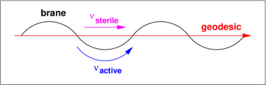
Figure 1: Schematic representation of a periodically curved brane in Minkowski spacetime. A coordinate transformation leads to an equivalent description as a non-diagonal metric with a flat brane, as described in the text.

In the spirit of [9] it is straightforward to construct a 1+1 dimensional toy model with a metric which indeed exhibits the anticipated behavior. First, write down a 1+2 dimensional embedding spacetime, with Minkowski metric

$${}ds^{2}=dt^{2}-dx^{2}-dy^{2}\,.$$ (1)

In this embedding spacetime, assume the brane exhibits periodic (for simplicity) oscillations in space

$${}y=A\,\sin kx\,;$$ (2)

see Fig. 1 for a schematic representation. Here $k$ is the wave number of the fluctuation (in the $x$-direction), and $A$ is the amplitude of the fluctuation (in the $y$-direction). A brane with tension is dynamical, and fluctuations change in time. The toy-model fluctuations should be thought of as some rms average over many time-slices.

The bulk-geodesic for the sterile neutrino is simply given by $y=0$, which leads to a travel distance of

$${}D_{g}=x\,.$$ (3)

The geodesic for the active state on the brane is slightly more complicated:

$${}D_{b}=\int_{\rm brane}\sqrt{dx^{2}+dy^{2}}=\int^{x}\sqrt{1+A^{2}k^{2}\cos^{2}kx}~{}dx\,.$$ (4)

We use subscripts $b$ and $g$ to denote the brane and bulk spaces, respectively.

In terms of the coordinate $x$, the parameter describing the shortcut in the bulk is

$${}\epsilon(x)=\frac{D_{b}-D_{g}}{D_{b}}=1-\frac{x}{\int^{x}\sqrt{1+A^{2}k^{2}\cos^{2}kx}~{}dx}\,.$$ (5)

While mathematically correct, this description of the geodesics as functions of $x$ has a shortcoming, in that $x$ is not a coordinate easily identified in an experiment on the brane. It is useful to consider a more physical set of brane coordinates. They will lead to essentially the same parameter $\epsilon$.

Consider the space-coordinate transformation

$${}u=y-A\,\sin kx$$ (6)

and

$${}z=\int^{x}\sqrt{1+A^{2}k^{2}\cos^{2}kx}~{}dx\,.$$ (7)

Under this transformation, the line element in (1) transforms into

$${}ds^{2}=dt^{2}-dz^{2}-du^{2}-\frac{2\,A\,k\,\cos kx(z)}{\sqrt{1+A^{2}k^{2}\cos^{2}kx(z)}}~{}du~{}dz.$$ (8)

Note that in $(u,z)$ coordinates, $u=0$ defines the location of the brane, and $z$ labels the physical distance along the brane. Consequently, a photon moving along the brane ($u=0$) satisfies the equation

$${}ds^{2}=dt^{2}-dz^{2}\,,$$ (9)

and thus travels in time $t_{f}$ the distance

$${}z_{b}=t_{f}\,.$$ (10)

On the other hand, in $(x,y)$ coordinates, the brane is described by the periodic sine function, while the geodesic in the bulk follows a straight line along mean $y$, given by

$${}y_{g}=0,~{}~{}~{}D_{g}=t.$$ (11)

Using eqs. (6) and (7), the bulk geodesic equation (11) can be transformed into the $(u,z)$ system,

$${}u_{g}=-A\,\sin(kt),$$ (12)

$${}z_{g}=\int_{0}^{t_{f}}\sqrt{1+A^{2}k^{2}\cos^{2}kt}~{}dt=\frac{\sqrt{1+A^{2}k^{2}}}{k}\,\,{\cal E}\left(kt_{f},\sqrt{\frac{A^{2}k^{2}}{1+A^{2}k^{2}}}\,\,\right),$$ (13)

where ${\cal E}(p,q)$ denotes the elliptic integral of the second kind.

The bulk geodesic intersects the brane at $u_{g}=0$, which according to eq. (12) occurs at the discrete times

$${}t_{\rm int}=\frac{n\pi}{k},$$ (14)

where $n$ is an integer. However, if the size of the brane’s fluctuations is small on the scale of an experimental detector, then it is not required that the two geodesics be in intersection, and $t_{\rm int}$ has no special significance.

From a comparison of the integrand in (13) to the result of (10), one readily infers that $z_{g}>z_{b}$, which means that in a common time interval the bulk test particle seemingly travels farther in the physical $z$-coordinate than the brane particle. In other words, the specific metric (8) allows apparent superluminal propagation. The shortcut in the bulk can be parametrized by

$${}\epsilon(t_{f})=\frac{z_{g}-z_{b}}{z_{g}}=1-\frac{k~{}t_{f}}{\sqrt{(1+A^{2}k^{2})}\,\,{\cal E}\left(k~{}t_{f},\sqrt{\frac{A^{2}k^{2}}{1+A^{2}k^{2}}}\,\right)}\,.$$ (15)

We note that this $\epsilon$ and the one defined in eq. (5) are formally the same when the space-coordinate $x$ is replaced by the physical time-coordinate $t$.

The parameter $\epsilon$ depends very weakly on $t_{f}$ when many fluctuations are traversed, i.e. when $t_{f}\gg 2\pi/k$. In fact, we are free to choose $t_{f}$ according to eq. (14). With this choice, the shortcut parameter depends only on the geometry $Ak$ of the brane fluctuation, according to

$${}\epsilon=1-\frac{\pi/2}{\sqrt{(1+A^{2}k^{2})}\,\,{\cal E}^{c}\left(\frac{\pi}{2},\sqrt{\frac{A^{2}k^{2}}{1+A^{2}k^{2}}}\,\right)}\,.$$ (16)

In the latter equation, we have used the relation ${\cal E}\left(n\pi,q\right)=2n\,{\cal E}^{c}\left(\frac{\pi}{2},q\right)$; the expression ${\cal E}^{c}\left(\frac{\pi}{2},q\right)$ is called the complete elliptic integral. In the model developed here, an inference of $\epsilon$ offers a direct measurement of the brane-fluctuation shape-parameter $Ak$.

The dimensionless ratio $Ak$ is essentially the aspect ratio (height to width) of the fluctuation. For a brane with high (low) tension, we expect a low (higher) value of $Ak$. Our assumption is that the brane tension is large, so that there is no curvature on large scales. Accordingly, we expect a small value for $Ak$. To first non-vanishing order in $Ak$, the parameter $\epsilon$ is

$${}\epsilon=\left(\frac{Ak}{2}\right)^{2}\,.$$ (17)

This approximation is valid until $Ak$ becomes of order unity, after which $z_{g}\gg z_{b}$ and $\epsilon$ itself approaches unity.

An alternative to the periodic metric described here arises in spacetimes in which the speed of light along flat 4D sections varies with the extra dimension coordinate $u$ due to different warp factors for the space and the time coordinates (“asymmetrically warped” spacetimes) [9, 10]. Such scenarios are realized, e.g. by a black-hole background in the bulk, and may provide interesting consequences for the adjustment of the cosmological constant [10]. A specific example is the two-brane scenario discussed in [9], in which the 4+1 dimensional metric is given by

$${}ds^{2}=dt^{2}-[e^{-2ku}a^{2}(t)\,d{\bf h}^{2}+du^{2}].$$ (18)

Here ${\bf h}$ denotes an Euclidian three-vector. In this model a sterile neutrino could scatter out of our brane at $u_{1}$ on a geodesic perpendicular to $h$, reach a second brane at $u_{2}>u_{1}$, and finally scatter off some fields confined on this second brane to return back to our brane. It has been shown in [9] that again the on-brane distance traveled in a given time interval via a path on the hidden-sector brane and in the bulk can be larger than the distance for pure on-brane travel in the same time interval. We anticipate that the qualitative features of this and similar scenarios can be approximated by the simple toy model discussed above.

3 The two-state sterile-active oscillation probability

Let us illustrate the brane-bulk resonance for a simple system of one sterile neutrino $\nu_{s}$ and one active neutrino $\nu_{a}$. The mass eigenstates are $m_{2}$ and $m_{1}$, respectively, in the sense that for small mixing $\nu_{s}$ is mostly $\nu_{2}$ and $\nu_{a}$ is mostly $\nu_{1}$.

Ignoring the bulk for the moment, the evolution equation in flavor space reads

$${}i\frac{d}{dt}\left(\begin{array}[]{c}\nu_{a}(t)\\ \nu_{s}(t)\end{array}\right)=H_{F}\left(\begin{array}[]{c}\nu_{a}(t)\\ \nu_{s}(t)\end{array}\right),$$ (19)

and the Hamiltonian in the flavor basis is

$${}H_{F}=E+\frac{1}{2}\,Tr+\frac{\delta m^{2}}{4\,E}\left(\begin{array}[]{rr}-\cos 2\theta&\sin 2\theta\\ \sin 2\theta&\cos 2\theta\\ \end{array}\right)$$ (20)

where $Tr=m_{2}^{2}+m_{1}^{2}/2E$, $\delta m^{2}=m_{2}^{2}-m_{1}^{2}$ and $\theta$ is the mixing-angle in the unitary matrix relating flavor and mass bases:

$${}|\nu_{\alpha}\rangle=U^{*}_{\alpha j}\,|\nu_{j}\rangle\,,\quad{\rm or}\quad U_{\alpha j}=\langle\nu_{\alpha}|\nu_{j}\rangle\,,$$ (21)

with

$${}U=\left(\begin{array}[]{rr}\cos\theta&\sin\theta\\ -\sin\theta&\cos\theta\\ \end{array}\right).$$ (22)

We will call $\theta$ and $\delta m^{2}$ the standard mixing angle, and standard mass-squared difference, respectively. They are the analogs of vacuum values in MSW [11] physics.

Now we let the sterile neutrino propagate in the bulk as well as on the brane. If the brane were rigid and flat in its embedding, then the sterile geodesic is just the same as the active geodesic on the brane. However, if the brane is curved in its embedding, as discussed above, then the sterile neutrino may have a different trajectory, with a shorter geodesic than that of the active neutrino constrained to the brane. We will formulate this as an effective potential contributing to the sterile-sterile term of the Hamiltonian in flavor space. Note that this is analogous to the Wolfenstein potential for the active-active term due to forward elastic scattering in matter, albeit with three important differences. The first is that the effective potential here is the same for neutrino and antineutrino, because gravitationally-determined geodesics do not distinguish between particle and antiparticle. The second difference is a more pronounced energy dependence here, with the effective mass-squared difference varying as $E^{2}$, not as $E$. The third difference is that there is no time or space dependence in the Hamiltonian. We note that characteristics of this brane-bulk luminal/superluminal system resemble certain scenarios with Lorentz invariance violation [12, 13].

Due to the shortcut in the bulk (see the schematic in Fig. (1)), the sterile state will appear to cover more distance on the brane than the active neutrino does in the same time, or equivalently, the same distance but in a shorter time. The ratio of apparent times at common distance or apparent distances at common time for the sterile and active neutrinos is $\delta t/t\simeq\delta z/z\simeq\epsilon$. For the toy model introduced in section 2 the parameter $\epsilon$ is given by eq. (16), or by eq. (17) to lowest non-vanishing order in $Ak$.

Adding the new contribution to the sterile-sterile element of the $H_{F}$, action/time$=E\,\frac{\delta t}{t}$, and then removing the irrelevant energy and trace terms, we arrive at the effective Hamiltonian

$${}H_{F}=+\frac{\delta m^{2}}{4\,E}\,\left(\begin{array}[]{rr}-\cos 2\theta&\sin 2\theta\\ \sin 2\theta&\cos 2\theta\\ \end{array}\right)+E\,\frac{\epsilon}{2}\,\left(\begin{array}[]{rr}1&0\\ 0&-1\\ \end{array}\right).$$ (23)

The bulk term may beat against the brane term to give resonant mixing, i.e., for some energy $E_{\rm res}$ even a small standard angle can become large or even maximal in the brane-bulk model. The resonance condition is that the two diagonal elements in $H_{F}$ be equal, which implies

$${}E_{\rm res}=\sqrt{\frac{\delta m^{2}\,\cos 2\theta}{2\,\epsilon}}\,.$$ (24)

Since the value of $\epsilon$ is unknown, the resonance energy could have almost any value, a priori. However, if $\epsilon\ll 1$, as we assume, then we have the result $\delta m^{2}\ll E^{2}_{\rm res}$. Still, there is much parameter space available for resonance. Our aim is to accommodate the LSND result in a four-neutrino framework, and so we will restrict the resonance energy with this in mind. It is worth noting that according to (24), a determination of $E_{\rm res}$ fixes $\epsilon$, if $\delta m^{2}$ and $\cos 2\theta$ can be independently determined. One way to independently determine $\delta m^{2}$ and $\cos 2\theta$ is to observe the active-sterile oscillation parameters far below resonance, where the oscillations are described by the standard formulas. Note that knowledge of $\epsilon$, when available, yields the shape-parameter $Ak$ of the brane fluctuation, according to eq. (17).

The value of $E_{\rm res}$ naturally divides the energy domain into three regions. Below the resonance, oscillation parameters reduce to their standard values and give the familiar oscillation results. At resonance, the mixing angle attains a maximum (but the effect on the oscillation probability can be reduced by a compensating factor in the $\delta m^{2}$ term). Above resonance, the oscillations are suppressed. Our strategy to accommodate the LSND data in a four-neutrino framework will be to set the resonant energy well below the CDHS data to suppress oscillations for this experiment, but at or above the LSND energies, so as to not suppress (or even, to enhance) the LSND signal.

To find the new eigenvalue difference $\delta H$ and the new mixing angle $\tilde{\theta}$ effected by the bulk, one diagonalizes the $2\times 2$ system. In terms of the new $\delta H$ and $\tilde{\theta}$ one obtains the usual expression for the flavor-oscillation probability

$${}P_{as}=\sin^{2}2\tilde{\theta}\;\sin^{2}(\delta H\,D/2)\,,$$ (25)

with new values given in terms of standard values by

$${}\sin^{2}2\tilde{\theta} = \frac{\sin^{2}2\theta}{\sin^{2}2\theta+\cos^{2}2\theta\left[1-\left(\frac{E}{E_{\rm res}}\right)^{2}\right]^{2}}\,,$$ (26)

$$\delta H = \frac{\delta m^{2}}{2\,E}\sqrt{\sin^{2}2\theta+\cos^{2}2\theta\left[1-\left(\frac{E}{E_{\rm res}}\right)^{2}\right]^{2}}\,.$$ (27)

The width of the resonance is easily derived from the classical amplitude in eq. (26). Fig. 2 shows $\sin^{2}2\tilde{\theta}$ for different values of $\sin^{2}2\theta$ as a function of energy.

Figure 2: Oscillation amplitude $\sin^{2}2\tilde{\theta}$ as a function of the neutrino energy $E_{\nu}$, for a resonance energy of $E_{\rm res}=40$ MeV. The different curves correspond to different values for the standard angle, $\sin^{2}2\theta=0.2,0.1,0.01,0.001$ (from above).

For $E\gg E_{\rm res}$, the sterile state decouples from the active state, as $\sin^{2}2\tilde{\theta}\rightarrow 0$. Although the example presented in this section contains a single sterile state and a single active state, the decoupling of the sterile state(s) from the active state(s) is a general feature.

4 Accommodating the LSND result

	$\alpha\beta$	$E_{\nu}$	$D$	$\sin^{2}2\tilde{\theta}_{\alpha\beta}$
LSND	$\mu e$	20-52.8 MeV	30 m	$>0.003$
KARMEN	$\mu e$	20-52.8 MeV	17.7 m	$<0.002$
MiniBooNE	$\mu e$	0.1-1.0 GeV	540 m	$\sim 0.0006$
BUGEY	${e\not{\!e}}$	1-6 MeV	25 m	$<0.15$
CDHS	${\mu\not{\!\mu}}$	$>1$ GeV	755 m	$<0.1$

Table 1: Flavor channels, beam energies, oscillation distances (or differences of far and near detectors), and limiting oscillation amplitudes in the large $\delta m^{2}$ limit, for the relevant experiments [6, 14, 15, 16, 17]. For BUGEY, the 25 m measurement has been chosen.

As the sterile neutrino mass is not protected by the gauge symmetry of the Standard Model, it is natural to assume it to be larger than the masses of the active neutrinos. We thus focus here on a $3+1$ neutrino spectrum [18], i.e. three active neutrinos are separated by the LSND mass-squared gap $\delta m^{2}_{\rm LSND}$ from the dominantly sterile state $\nu_{4}\sim\nu_{s}$.

In the present model, $\delta\tilde{m}^{2}_{\rm LSND}$ differs from the standard formalism by the square-root factor in (27). If the new resonance occurs in the energy range of LSND/KARMEN, this factor might allow a fit with a larger $\delta m^{2}$. We do not pursue this subtlety in this work (see, however, the discussion in section 5.2).

For short distances, the mass-squared differences in the $3+1$ spectrum can be taken as $\delta m^{2}\equiv\delta m^{2}_{14}=\delta m^{2}_{24}=\delta m^{2}_{34}$, with all other differences set to zero. There results in all short-distance oscillation probabilities a universal factor of $\sin^{2}(\delta H~{}D/2)$, with $\delta H$ given previously in eq. (27). As a result of this universality, the relevant oscillation amplitudes can be completely described using a two-neutrino formulation. First, we define the linear combination of active flavors which couples to the heavy $|\nu_{4}\rangle$ mass eigenstate as $|\nu_{a}\rangle$. Below the resonant energy, we write

$${}|\nu_{4}\rangle=\cos\tilde{\theta}|\nu_{s}\rangle+\sin\tilde{\theta}|\nu_{a}\rangle\,.$$ (29)

Above the resonant energy, the mass eigenstates have to be relabeled ($4\leftrightarrow 1$); i.e. the isolated state contains little $|\nu_{a}\rangle$ but much $|\nu_{s}\rangle$. Put another way, the oscillations considered still occur above the resonance over the large active-sterile mass gap, but effectively with the interchange $\cos\tilde{\theta}\leftrightarrow\sin\tilde{\theta}$ in eq. (29). We note that $\sin^{2}2\tilde{\theta}$ is unaffected by this interchange.

To produce $\nu_{\mu}$-$\nu_{e}$ oscillations, it is necessary that this state $|\nu_{a}\rangle$ contains $|\nu_{\mu}\rangle$ and $|\nu_{e}\rangle$. It may also contain $|\nu_{\tau}\rangle$. For simplicity, we will take this state to be a mixture of just $|\nu_{\mu}\rangle$ and $|\nu_{e}\rangle$:

$${}|\nu_{a}\rangle=\cos\theta_{*}|\nu_{\mu}\rangle+\sin\theta_{*}|\nu_{e}\rangle\,.$$ (30)

Thus, we have

$${}\tilde{U}_{e4} = \sin\tilde{\theta}\,\sin\theta_{*}\,,$$ (31)

$$\tilde{U}_{\mu 4} = \sin\tilde{\theta}\,\cos\theta_{*}\,,$$ (32)

below the resonant energy, and $\cos\tilde{\theta}\leftrightarrow\sin\tilde{\theta}$ in eqs. (31) and (32) above the resonant energy.

The oscillation amplitude relevant for the LSND [6], KARMEN [14] and MiniBooNE [15] appearance experiments is given by

$${}\sin^{2}2\tilde{\theta}_{\rm LSND}=-4\sum_{j<4}\tilde{U}_{e4}\,\tilde{U}_{\mu 4}\,\tilde{U}_{ej}\,\tilde{U}_{\mu 4}=4\,\tilde{U}_{e4}^{2}\,\tilde{U}_{\mu 4}^{2}=\sin^{2}2\theta_{*}\,\sin^{4}\tilde{\theta}\,.$$ (33)

Similarly, the oscillation amplitudes for the $\nu_{e}$ and $\nu_{\mu}$ disappearance experiments BUGEY [16] and CDHS [17] are given by

$${}\sin^{2}2\tilde{\theta}_{e\not{e}} = 4\,\tilde{U}_{e4}^{2}\,(1-\tilde{U}_{e4}^{2})=4\,\sin^{2}\tilde{\theta}\sin^{2}\theta_{*}\,(1-\sin^{2}\tilde{\theta}\sin^{2}\theta_{*}),$$ (34)

$$\sin^{2}2\tilde{\theta}_{\mu\not{\mu}} = 4\,\tilde{U}_{\mu 4}^{2}\,(1-\tilde{U}_{\mu 4}^{2})=4\,\sin^{2}\tilde{\theta}\cos^{2}\theta_{*}\,(1-\sin^{2}\tilde{\theta}\cos^{2}\theta_{*}),$$ (35)

respectively. The far-right expressions in these equations hold below the resonance; above the resonance one must interchange $\cos\tilde{\theta}\leftrightarrow\sin\tilde{\theta}$, as explained above.

Eq. (34) may be inverted to give $\tilde{U}_{e4}^{2}=\sin^{2}\tilde{\theta}_{e\not{e}}$, and eq. (35) to give $\tilde{U}_{\mu 4}^{2}=\sin^{2}\tilde{\theta}_{\mu\not{\mu}}$. Were these probabilities not energy-dependent, as in the standard vacuum case, one could substitute these results into eq. (33) to get

$${}\sin^{2}2\theta_{\rm LSND}=4\,\sin^{2}\tilde{\theta}_{e\not{e}}\sin^{2}\tilde{\theta}_{\mu\not{\mu}}\simeq\frac{1}{4}\sin^{2}2\theta_{e\not{e}}\sin^{2}2\theta_{\mu\not{\mu}}\,,$$ (36)

with the latter expression holding in the small angle approximation. One recovers the well-known result in the standard case, that the LSND amplitude is doubly suppressed by stringent bounds on the BUGEY and CDHS amplitudes. This fact excludes the standard 3+1 neutrino models from describing the results of all short-baseline neutrino experiments [19]. However, eq. (36) is not valid in general in our bulk shortcut scenario. As we shall demonstrate, the energy-dependence imparted to the mixing-angles and to $\delta H$ by the bulk shortcut allows consistency.

It will also be useful to list the amplitudes for $\nu_{\mu}$-$\nu_{s}$ and $\nu_{e}$-$\nu_{s}$ oscillations, for these may affect atmospheric and solar oscillations. As shown in eqs. (26,27), the active-sterile oscillations are governed by vacuum values below the resonant energy, are maximal at the resonant energy, and are suppressed above the resonant energy. The same is true therefore for $\nu_{\mu}$-$\nu_{s}$ and $\nu_{e}$-$\nu_{s}$ oscillations:

$${}\sin^{2}2\tilde{\theta}_{\mu s}=\cos^{2}\theta_{*}\,\sin^{2}2\tilde{\theta}\,,$$ (37)

and

$${}\sin^{2}2\tilde{\theta}_{es}=\sin^{2}\theta_{*}\,\sin^{2}2\tilde{\theta}\,,$$ (38)

with $\sin^{2}2\tilde{\theta}$ given in eq. (26).

For the analysis of neutrino oscillations in the bulk-shortcut scenario, the energy of the neutrino beam is of crucial importance. In Table 1, the relevant experiments are shown together with the flavor amplitude to which they are sensitive, the neutrino beam energy, and the bound (or for LSND, the favored region) for the amplitude. Our task is to compare these experimental bounds (and for LSND, the positive signal) with the energy-dependent oscillation probabilities listed above. Note that all experimental data must be accommodated with four parameters: the standard mass-squared difference $\delta m^{2}$, the standard mixing angles $\theta$ (describing $\nu_{a}$-$\nu_{s}$ mixing) and $\theta_{*}$ (parametrizing the flavor composition of $\nu_{a}$), and the shortcut parameter $\epsilon$ (or equivalently, the resonant energy $E_{R}$, as given in eq. (24)).

4.1 BUGEY

BUGEY detects reactor neutrinos of energies an order of magnitude below the energies of LSND. We assume that the BUGEY energies are also far below the resonance energy, in which case the bulk shortcut effects decouple and the oscillation amplitude is given by the standard limit of eq. (34),

$${}\sin^{2}2\theta_{e\not{e}}\simeq 4\,U_{e4}^{2}\simeq 4\,\sin^{2}\theta\,\sin^{2}\theta_{*}.$$ (39)

Here the smallness of $\sin^{2}2\theta_{e\not{e}}$ has been assumed, in concordance with the BUGEY limit $\sin^{2}2\theta_{e\not{e}}<0.15$. We note that the BUGEY amplitude maybe suppressed by a small $\sin^{2}\theta_{*}$, or small $\sin^{2}\theta$, or both.

In the following we discuss two parameterizations compatible with LSND and CDHS which sufficiently suppress this BUGEY amplitude, namely $\sin^{2}2\theta=0.9$, $\sin^{2}\theta_{*}=0.01$, and $\sin^{2}2\theta=0.45$, $\sin^{2}\theta_{*}=0.1$. The first parameterization has a large active-sterile mixing, $\theta=36^{\circ}$, but still a small $\sin^{2}2\theta_{e\not{e}}=0.014$. The second parameterization yields a moderate $\theta=21^{\circ}$ and small $\sin^{2}2\theta_{e\not{e}}=0.052$. Since the BUGEY amplitude is sufficiently suppressed, there is no bound from BUGEY data on the value of $\delta m^{2}$.

Future reactor experiments are proposed to search for nonzero $U_{e3}$. In these experiments, mixing of the sterile state with $\nu_{e}$ would have a measurable effect, mimicking a non-zero $U_{e3}$. In contrast to the effects of a non-zero $U_{e3}$ (equivalently, a non-zero $\theta_{13}$) and as a result of the large oscillation phase $\propto\delta m^{2}_{\rm LSND}$, the effect will be seen in both the near and the far detectors, though, and can be as large as $\sin^{2}2\theta_{13}=0.05$.

4.2 CDHS

The accelerator oscillation experiment CDHS operated with neutrino energies above a GeV. At energies $E\gg E_{\rm res}$ the active-sterile mixing is suppressed, and one can approximate for small $\sin\theta_{*}$ (from eqs. (26) and (35))

$${}\sin^{2}2\tilde{\theta}_{\mu\not{\mu}}\simeq\cos^{2}\theta_{*}\,\sin^{2}2\tilde{\theta}\simeq\cos^{2}\theta_{*}\tan^{2}2\theta\left(\frac{E}{E_{\rm res}}\right)^{-4}\,.$$ (40)

This implies that neutrino oscillations in the CDHS experiment are suppressed by a factor between $10^{6}$ and 40 for a resonance energy in the range of 30-400 MeV, making the oscillation amplitude $\sin^{2}2\theta_{\mu\not{\mu}}$ unobservable above $\sim$ GeV, even if the $\sin^{2}2\theta_{\mu\not{\mu}}$ were maximal below the resonance.

4.3 LSND and KARMEN

We have suppressed the BUGEY oscillation amplitude with the choice of a small $U_{e4}^{2}$ below resonance. We have suppressed the CDHS oscillation amplitude with the choice of a resonant energy below 400 MeV. This leaves two possibilities for the effect of the resonance on the LSND/KARMEN energy range, 20-53 MeV. The resonance may occur within this range, in which case the effect is observable. Alternatively, the resonance may occur above this range, in which case there is little change from the standard prediction and fit. We show below that either possibility can be realized with a resonance consistent with all other oscillation data. We also show below that the two different choices have very different consequences for the on-going MiniBooNE experiment.

From eq. (33) and the following discussion, we have for the LSND oscillation amplitude

$${}\sin^{2}2\tilde{\theta}_{\rm LSND}=\frac{1}{4}\sin^{2}2\theta_{*}\,(1\mp\cos 2\tilde{\theta})^{2}\,.$$ (41)

The sign of the $\cos 2\tilde{\theta}$ term corresponds to energies below and above $E_{\rm res}$, respectively, accounting for the fact that the states have to be relabeled when crossing the resonance so that the oscillations considered occur over the large active-sterile mass gap. This formula also applies for the KARMEN and MiniBooNE amplitudes.

In Figs. (3) and (4) the oscillation probability $P_{\mu e}$ predicted for LSND in the bulk-shortcut scenario is compared to the prediction of the standard oscillation case (dashed). Also shown is the expectation for KARMEN. Two very different sets of parameters have been chosen: one scenario has a resonant energy $E_{\rm res}=33$ MeV in the LSND/KARMEN energy range, and the other has a resonant energy $E_{\rm res}=400$ MeV far beyond the LSND/KARMEN energy range.

To maintain consistency between the LSND and KARMEN data, it is necessary to exploit the differing distances of the two experimental configurations, $D_{\rm LSND}=30$ m and $D_{\rm KARMEN}=17.7$ m according to Table 1. As in the standard approach, this is done as follows: According to eq. (25), the neutrino remains in its first oscillation until $\delta H\,D=2\,\pi$. For $\delta H\,D\ll 2\,\pi$, the factor $\sin^{2}(\delta H\,D/2)$ is well approximated by just $(\delta H\,D/2)^{2}$, giving oscillation probabilities a quadratic dependence on distance. Since the baseline for KARMEN is about half that of LSND, choosing parameters such that $\delta H\,D_{\rm KARMEN}\raise 1.29167pt\hbox{$\;<$\kern-7.5pt\raise-4.73611pt\hbox{$\sim\;$}}1$, with $\delta H$ given in eq. (27), suppresses KARMEN by a factor of four compared to LSND. This allows a slice of LSND parameter space to remain viable, in the face of the KARMEN null result.

The requirement for LSND/KARMEN neutrinos to remain within their first oscillation is the standard one, $\delta m^{2}\sim{\rm eV}^{2}$. We adopt this value here.

At this point, we may invert eq. (24) to determine the value of $\epsilon$:

$${}\epsilon=\frac{\cos 2\theta\,\delta m^{2}}{2\,E_{\rm res}^{2}}=\frac{\cos 2\theta}{2}\,\left(\frac{\delta m^{2}}{{\rm eV}^{2}}\right)\,\left(\frac{100\,{\rm MeV}}{E_{\rm res}}\right)^{2}\times 10^{-16}\,.$$ (42)

The freedom for $E_{\rm res}$ in this model allows $\epsilon$ to range over $\sim 10^{-18}$ to $10^{-16}$. According to eq. (17), this in turn implies a shape-parameter (height to width ratio) for the brane fluctuation of $Ak\sim 10^{-8}$. These parameter values have to be eventually explained in a theory of brane dynamics.

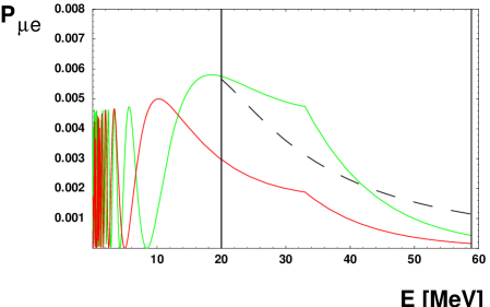
Figure 3: Bulk shortcut oscillation probabilities for LSND (light/green) and KARMEN (dark/red) as a function of the neutrino energy. Shown is a scenario with $E_{\rm res}=33$ MeV; $\sin^{2}\theta_{*}=0.01$; $\sin^{2}2\theta=0.9$; $\delta m^{2}=0.7$ eV². For comparison, a standard oscillation probability for LSND ($\delta m^{2}=0.8$ eV, $\sin^{2}2\theta_{\rm LSND}=0.006$) is displayed (dashed). The vertical lines indicate the energy window of LSND and KARMEN.

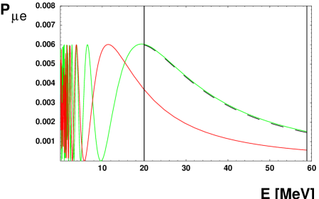
Figure 4: Bulk shortcut oscillation probabilities for LSND (light/green) and KARMEN (dark/red) as a function of the neutrino energy. Shown is a scenario with $E_{\rm res}=400$ MeV, $\sin^{2}\theta_{*}=0.1$; $\sin^{2}2\theta=0.45$; $\delta m^{2}=0.8$ eV². For comparison, a standard oscillation probability ($\delta m^{2}=0.8$ eV, $\sin^{2}2\theta_{\rm LSND}=0.006$) for LSND is displayed (dashed). The vertical lines indicate the energy window of LSND and KARMEN.

Both choices for $E_{\rm res}$ exhibit a viable LSND energy spectrum, as seen in the figures. For the case where $E_{\rm res}\gg E_{\rm LSND}$, the LSND/KARMEN analysis and fit is the standard one. For the case where $E_{\rm res}$ lies in the LSND range 20 MeV$<E<53$ MeV, the energy dependence of the oscillation amplitude is modified considerably. For this latter case, we expect that the resonance should be evident in the LSND spectral data, and we encourage a re-analysis of the measured LSND energy-spectrum by the collaboration.

4.4 Solar and Atmospheric Data

The active-sterile amplitudes for $\nu_{\mu}$ and $\nu_{e}$ are given in eqs. (37) and (38). However, the same physics which suppresses active-sterile oscillations in BUGEY data and CDHS data, also suppresses active-sterile oscillations in solar and atmospheric data, respectively. For solar oscillations, the smallness of $|U_{e4}|^{2}$ evades the experimental constraint. For atmospheric neutrinos, the measured energies are above the resonant energy, and so atmospheric oscillations into the sterile state are suppressed. The event sample below 500 MeV may contain enhanced $\nu_{s}$ production, but experimentally this would be difficult to confirm.

In fact, even the 2+2 model of four-neutrinos can be resurrected with the brane-bulk resonance. In the same way that the suppression of sterile-active oscillations above the resonant energy neutralizes the CDHS constraint for the 3+1 model, so does it neutralize the atmospheric constraint for the 2+2 model.

A detailed calculation is required to determine the nearly unitary $3\times 3$ active-neutrino mixing-matrix that results when the sterile state decouples at high energy. We do not pursue this here. However, we expect that the freedom to partition the state $|\nu_{a}\rangle$ among the $|\nu_{e}\rangle$, $|\nu_{\mu}\rangle$, and $|\nu_{\tau}\rangle$ is sufficient to yield acceptable phenomenology. For example, although we have taken $\langle\nu_{\tau}|\nu_{a}\rangle=0$ for simplicity, a $\nu_{\mu}\leftrightarrow\nu_{\tau}$ interchange symmetry, known to be consistent with all present data, can be incorporated here by changing $|\nu_{\mu}\rangle$ in eq. (30) to $|\nu_{\mu}^{\prime}\rangle=\frac{1}{\sqrt{2}}(|\nu_{\mu}\rangle+|\nu_{\tau}\rangle)$.

4.5 MiniBooNE

The requirement that $E_{\rm res}\raise 1.29167pt\hbox{$\;<$\kern-7.5pt\raise-4.73611pt\hbox{$\sim\;$}}400$ MeV, well below the CDHS energy of $\sim 1$ GeV, leaves the resonance energy in the MiniBooNE range, 0.1 to 1 GeV, or even below. We predict that MiniBooNE should see no signal above $\sim 700$ MeV in this model.

If $E_{\rm res}$ falls in the MiniBooNE range above 100 MeV, then MiniBooNE should observe a strongly enhanced signal as evidence for the bulk-shortcut resonance. Near the resonance region, the exact expression (41) applies for MiniBooNE. Results of this expression are shown in Fig. 5 for resonance energies of 200, 300 and 400 MeV. As can be seen, the strongly enhanced oscillation probability is unmistakable.

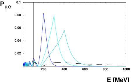
Figure 5: Bulk shortcut oscillation probabilities for MiniBooNE as a function of the neutrino energy. Shown is a scenario with $\sin^{2}\theta_{*}=0.1$; $\sin^{2}2\theta=0.45$; $\delta m^{2}=0.8$ eV². The resonance energy is varied, $E_{\rm res}=200,~{}300,~{}400$ MeV, from left to right (light to dark). For comparison, the expectation for a standard oscillation solution ($\delta m^{2}=0.8$ eV, $\sin^{2}2\theta_{\rm LSND}=0.006$) for LSND is displayed (dashed). The vertical line indicates the energy threshold of MiniBooNE.

On the other hand, if $E_{\rm res}$ lies below the MiniBooNE threshold energy, then active-sterile mixing is strongly suppressed for MiniBooNE. At energies $E\gg E_{\rm res}$, one uses eq. (26) in eq. (41) to approximate

$${}\sin^{2}2\tilde{\theta}_{\rm MiniBooNE}\simeq\frac{1}{16}\sin^{2}2\theta_{*}\tan^{4}2\theta\left(\frac{E}{E_{\rm res}}\right)^{-8}.$$ (43)

Thus a null result is predicted for MiniBooNE in the case of a resonance energy (as in our 33 MeV example) below the MiniBooNE threshold of ${\cal O}(100)$ MeV.

However, if $E_{\rm res}$ is too low for an observable effect in MiniBooNE, a distortion in the LSND spectrum is expected (see Fig. 3). A strong $\nu_{\mu}$ disappearance signal also is predicted for an experiment using neutrinos from stopped pions, being proposed for the Spallation Neutron Source (SNS). This we discuss next.

4.6 Muon-neutrino disappearance at the SNS

While the sterile neutrino effectively decouples from the active sector at the CDHS energy and above, there is no suppression of the active-sterile mixing at and below the resonance. Therefore, a significant effect is predicted for $\nu_{\mu}$ disappearance at lower energies.

Just such a lower energy $\nu_{\mu}$ disappearance experiment has been proposed [20] at the Spallation Neutron Source (SNS) being built at Oak Ridge. The neutrino source would be stopped $\pi^{+}$’s, which undergo two-body decay to produce a monochromatic $\nu_{\mu}$ beam at 30 MeV. In addition to the SNS source for stopped pions, there is the possibilty of a high-intensity “proton driver” at Fermilab which would also include stopped pions on its physics agenda. Detector distances at either site would be under 100 m from the pion source. Thus, the $D/E$ is sufficiently small that only the LSND $\delta m^{2}$ can effect neutrino flavor change.

The amplitude for $\nu_{\mu}$-survival is given by eq. (35), and the term oscillating with distance is $\sin^{2}(\delta H\,D/2)$, with $\delta H$ given in eq. (27). The effects predicted for the stopped-pion $\nu_{\mu}$ source at the SNS are shown in Fig. (6). The depletion of the $\nu_{\mu}$ beam due to substantial low-energy sterile-active mixing is considerable. For $E\ll E_{\rm res}$, or for $\theta$ near maximal, the oscillation length is insensitive to $E_{\rm res}$. This explains the nearly common distance for the various minima in the figure.

We note that the large $\nu_{\mu}$-depletion in Fig. (6) is specific to the parameters we have chosen, and so should be interpreted as illustrative only. Smaller mixing leads to smaller depletion. If a $\nu_{\tau}$ component were added to the $\nu_{a}$ state, the $\nu_{\mu}$-depletion may be less. Nevertheless, observable depletion of $\nu_{\mu}$’s from stopped pions is one of the more robust predictions of the brane-bulk model.

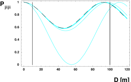
Figure 6: The muon-neutrino survival probability versus distance, for a monochromatic neutrino-beam energy of 30 MeV from stopped pions. The solid curves are parametrised by resonance energies 33, 100, 200 (identical for 300 and 400 MeV), in order of decreasing depletion. The dashed curve is the result with no bulk shortcut. The low-energy parameters for the 33 MeV resonance are chosen as in Fig. 3: $\sin^{2}\theta_{*}=0.01$; $\sin^{2}2\theta=0.9$; $\delta m^{2}=0.7$ eV²; while the parameters for the other curves are chosen as in Fig. 4: $\sin^{2}\theta_{*}=0.1$; $\sin^{2}2\theta=0.45$; $\delta m^{2}=0.8$ eV². The vertical lines indicate the range of possible source to near/far detector distances.

5 Further implications for astrophysics and cosmology

5.1 BBN

Successful big-bang nucleosynthesis puts severe constraints on the equilibration between active neutrinos and even a single sterile state, in the early Universe. The impact of active-sterile neutrino mixing on nucleosynthesis is quite complex. It has been discussed extensively, most recently in [21]. A popular idea to resurrect LSND in view of the BBN constraints is to introduce a lepton asymmetry, which gives effective masses to the active neutrinos in medium in the early universe, thus reducing the effective active-sterile matter mixing angles.

The bulk shortcut effect will further differentiate the sterile and active neutrinos. It also may provide an alternative to a lepton asymmetry. Consider natural expectations for the evolution of the brane metric: A higher density in the early universe will lead to greater gravitational attraction, and so to more brane buckles; and a larger temperature will increase thermal fluctuations of the brane. At the epoch of BBN, the temperature is ten orders of magnitude larger than today, and densities are thirty orders of magnitude larger than today. In the alternative metric (18) mentioned earlier, a higher density of scattering sites will increase the sterile neutrino scattering off from our brane. All these effects will increase the bulk shortcut parameter $\epsilon$ and thus reduce the resonance energy ($E_{\rm res}\propto 1/\sqrt{\epsilon}$). If $E_{\rm res}$ is reduced to a temperature near enough the BBN temperature of $\sim 3$ MeV, earlier oscillations will be suppressed. Our arguments that shortcuts had a larger $\epsilon$ and therefore smaller $E_{\rm res}$ in the earlier Universe are consistent with Ishihara’s statement, that the magnitude of apparent causality violation on the brane increases with increasing matter density [7].

5.2 Sterile neutrino mass and dark matter

The present scenario offers an effective mechanism for sterile neutrino production in the early Universe: when the temperature of the early universe drops below the resonant energy, the active-sterile mixing becomes maximal and active neutrinos are resonantly converted into sterile neutrinos. Afterwords, active neutrinos are re-populated via reactions maintaining thermodynamic equilibrium, until the active neutrinos decouple at energies around 1 MeV. The net effect, then, is to populate all neutrino modes, sterile and active.

The occupation of states for a sterile neutrino with mass in the eV range impacts the effective total neutrino mass and number, which in turn impacts the connection (“transfer function”) between the cosmic microwave background anisotropy and today’s large-scale structure. A similar impact of neutrino mass/energy obtains for measurements of galaxy bias stemming from galaxy-galaxy lensing, and for the large-scale power spectrum inferred from Lyman-alpha forest observations in the Sloan Digital Sky Survey. Specific consequences for cosmological evolution requires a detailed analysis (for recent works see [23]). Here we just mention that, as described in the previous subsection 5.1, higher temperatures and densities in the early universe may affect brane dynamics in a way to increase the effective shortcut parameter and to reduce the resonant energy. This effect may keep the sterile neutrino decoupled until the neutrino populations freeze out.

Since the effective $\delta\tilde{m}_{\rm LSND}^{2}\sim{\rm eV}^{2}$ is equal to $\sim\delta m^{2}_{\rm LSND}\sin 2\theta$ on resonance, the true $\delta m^{2}_{\rm LSND}$ can be larger by $1/\sin 2\theta$. In the case of a small mixing-angle, the gain can be very large. With a sufficiently small $\theta$, the LSND sterile neutrino could play an important role as warm dark matter (WDM) with a mass of order keV. WDM has been proposed to solve the cuspy core problem of cold dark matter scenarios [24]. Sterile WDM has also been proposed to induce the observed high-velocities of radio pulsars [25]. Unfortunately, it seems difficult to fit the actual LSND energy spectrum with a small mixing-angle $\theta$, as the required small mixing angles inducing sharp peaks at the resonance energy, see Fig. 2.

5.3 Supernova neutrinos

Oscillations into sterile bulk neutrinos have interesting consequences for supernova neutrinos. For example, supernova cooling may be accelerated due to the emission of Kaluza-Klein excitations of the sterile neutrino, resulting in constraints on a product involving the sterile-active neutrino mixing and the radius of the extra dimension and/or a delayed explosion process [26]. Since the efficiency of the bulk shortcut mechanism depends on the shortcut parameter $\epsilon\simeq\left(\frac{Ak}{2}\right)^{2}$ with only $A$ being bounded from the radius of the extra dimension, such constraints can always be avoided by choosing a smaller $A$ and a larger $k$.

Furthermore, oscillations into sterile neutrinos would affect r-process nucleosynthesis, i.e. the rapid capture of neutrons on iron-sized seed nuclei, which is the prime candidate for the synthesis of nuclei heavier than iron. This process, which is believed to occur in type II supernovae, is suppressed by $\nu_{e}$-capture on neutrons, which transforms the target neutrons into protons, forming stable $\alpha$ particles. It has been shown that $\nu_{e}$-capture can be suppressed sufficiently if $\nu_{e}$’s oscillate strongly into sterile neutrinos [27].

The bulk shortcut scenario will change this picture of r-process nucleosynthesis slightly. First, resonances, now involving matter effects and bulk effects, may find their energies shifted toward smaller values by the bulk shortcut. Moreover, supernova neutrinos with energies above the brane-bulk resonance will not experience any level-crossing when propagating out of the supernova, resulting in a cutoff of the active-sterile neutrino oscillation probability above $E_{\rm res}$.

5.4 Horizon problem

Finally, the sterile neutrino could couple more strongly to brane fields than the graviton, especially in the resonance region around $E_{\rm res}$. Thus, a solution to the horizon and homogeneity problems, proposed in [8, 9] but based on gravitons, might turn out to be more effective if based on sterile neutrinos. Moreover, while bounds on the size of extra dimensions from precision measurements of the gravitational force law [28] impose stringent constraints on the gravitational horizon, these bounds may not be valid for the extra dimensions felt by sterile neutrinos. The sterile neutrino horizon thus may be even larger than the gravitational horizon. Finally we stress that time dilation effects between the brane exit and the brane re-entry points can lead to causality violations which increase the sterile neutrino horizon. Such effects will be discussed in a forthcoming paper [29].

6 Discussion and Conclusions

We have discussed active-sterile neutrino oscillation in an extra-dimensional brane world scenario. In such scenarios, sterile neutrinos paths may take shortcuts in the bulk, which imparts an energy dependence to the oscillation amplitude. Resonant enhancement of active-sterile neutrino mixing arises, parameterized by a shortcut parameter $\epsilon\equiv\delta t/t$. If the resonant energy lies in the range 30 MeV to 400 MeV, suitably chosen between the BUGEY and CDHS energies, then all neutrino oscillation data can be accommodated in a consistent 3+1 neutrino framework. Such an energy range corresponds to $\epsilon$ in the range $10^{-18}-10^{-16}$, and to brane fluctuations with a height to width ratio of $\sim 10^{-8}$. The resonant energy might be identifiable in either the LSND spectral data and the muon neutrino disappearance from a stopped-pion source, or in the soon-to-appear MiniBooNE data.

There are further interesting consequences for neutrino physics. We have mentioned that even the 2+2 model of active-sterile mixing can be resurrected with the brane-bulk resonance. Finally, we have sketched only briefly several interesting consequences for astrophysics and cosmology, consequences which remain to be worked out in detail.

References

- [1] N. Arkani-Hamed, S. Dimopoulos and G. R. Dvali, The hierarchy problem and new dimensions at a millimeter, Phys. Lett. B 429, 263 (1998) [arXiv:hep-ph/9803315]; I. Antoniadis, N. Arkani-Hamed, S. Dimopoulos and G. R. Dvali, New dimensions at a millimeter to a Fermi and superstrings at a TeV, Phys. Lett. B 436, 257 (1998) [arXiv:hep-ph/9804398]; N. Arkani-Hamed, S. Dimopoulos and G. R. Dvali, Phenomenology, astrophysics and cosmology of theories with sub-millimeter dimensions and TeV scale quantum gravity, Phys. Rev. D 59, 086004 (1999) [arXiv:hep-ph/9807344].
- [2] L. Randall and R. Sundrum, A large mass hierarchy from a small extra dimension, Phys. Rev. Lett. 83, 3370 (1999) [arXiv:hep-ph/9905221]; L. Randall and R. Sundrum, An alternative to compactification, Phys. Rev. Lett. 83, 4690 (1999) [arXiv:hep-th/9906064]; N. Arkani-Hamed, S. Dimopoulos, G. R. Dvali and N. Kaloper, Infinitely large new dimensions, Phys. Rev. Lett. 84, 586 (2000) [arXiv:hep-th/9907209].
- [3] D. Cremades, L. E. Ibanez and F. Marchesano, Standard model at intersecting D5-branes: Lowering the string scale, Nucl. Phys. B 643, 93 (2002) [arXiv:hep-th/0205074]; C. Kokorelis, Exact standard model structures from intersecting D5-branes, Nucl. Phys. B 677, 115 (2004) [arXiv:hep-th/0207234].
- [4] N. Arkani-Hamed, S. Dimopoulos, G. R. Dvali and J. March-Russell, Neutrino masses from large extra dimensions, Phys. Rev. D 65, 024032 (2002) [arXiv:hep-ph/9811448]; K. R. Dienes, E. Dudas and T. Gherghetta, Light neutrinos without heavy mass scales: A higher-dimensional seesaw mechanism, Nucl. Phys. B 557, 25 (1999) [arXiv:hep-ph/9811428]; Y. Grossman and M. Neubert, Neutrino masses and mixings in non-factorizable geometry, Phys. Lett. B 474, 361 (2000) [arXiv:hep-ph/9912408]; S. J. Huber and Q. Shafi, Majorana neutrinos in a warped 5D standard model, Phys. Lett. B 544, 295 (2002) [arXiv:hep-ph/0205327].
- [5] For overviews of sterile neutrino physics, see, e.g., M. Cirelli, G. Marandella, A. Strumia, and F. Vissani, Probing oscillations into sterile neutrinos with cosmology, astrophysics and experiments, Nucl. Phys. B708, 215 (2005) [ArXiv:hep-ph/0403158]; R. Volkas, Introduction to sterile neutrinos, Prog. Part. Nucl. Phys. 48, 161 (2002) [ArXiv:hep-ph/0111326].
- [6] C. Athanassopoulos et al. [LSND Collaboration], Evidence for anti-nu/mu anti-nu/e oscillation from the LSND experiment at the Los Alamos Meson Physics Facility, Phys. Rev. Lett. 77, 3082 (1996) [arXiv:nucl-ex/9605003]; A. Aguilar et al. [LSND Collaboration], Evidence for neutrino oscillations from the observation of anti-nu/e appearance in a anti-nu/mu beam, Phys. Rev. D 64, 112007 (2001) [arXiv:hep-ex/0104049].
- [7] H. Ishihara, Causality of the brane universe, Phys. Rev. Lett. 86, 381 (2001) [arXiv:gr-qc/0007070].
- [8] G. Kaelbermann, Communication through an extra dimension, Int. J. Mod. Phys. A 15, 3197 (2000) [arXiv:gr-qc/9910063]. G. Kaelbermann and H. Halevi, Nearness through an extra dimension, arXiv:gr-qc/9810083.
- [9] D. J. H. Chung and K. Freese, Cosmological challenges in theories with extra dimensions and remarks on the horizon problem, Phys. Rev. D 61, 023511 (2000) [arXiv:hep-ph/9906542]; D. J. H. Chung and K. Freese, Can geodesics in extra dimensions solve the cosmological horizon problem?, Phys. Rev. D 62, 063513 (2000) [arXiv:hep-ph/9910235].
- [10] C. Csaki, J. Erlich and C. Grojean, Gravitational Lorentz violations and adjustment of the cosmological constant in asymmetrically warped spacetimes, Nucl. Phys. B 604, 312 (2001) [arXiv:hep-th/0012143].
- [11] L. Wolfenstein, Neutrino Oscillations In Matter, Phys. Rev. D 17, 2369 (1978); S. P. Mikheev and A. Y. Smirnov, Resonant Amplification Of Neutrino Oscillations In Matter And Solar Neutrino Spectroscopy, Nuovo Cim. C 9, 17 (1986); S. P. Mikheev and A. Y. Smirnov, Resonance Enhancement Of Oscillations In Matter And Solar Neutrino Spectroscopy, Sov. J. Nucl. Phys. 42, 913 (1985) [Yad. Fiz. 42, 1441 (1985)]; V. D. Barger, K. Whisnant, S. Pakvasa and R. J. N. Phillips, Matter Effects On Three-Neutrino Oscillations, Phys. Rev. D 22, 2718 (1980).
- [12] V. A. Kostelecky and M. Mewes, Lorentz violation and short-baseline neutrino experiments, Phys. Rev. D 70, 076002 (2004) [arXiv:hep-ph/0406255].
- [13] F. R. Klinkhamer, Lorentz-noninvariant neutrino oscillations: Model and predictions, arXiv:hep-ph/0407200; S. L. Glashow, Atmospheric neutrino constraints on Lorentz violation, arXiv:hep-ph/0407087. A. Datta, R. Gandhi, P. Mehta and S. U. Sankar, Atmospheric neutrinos as a probe of CPT and Lorentz violation, Phys. Lett. B 597, 356 (2004) [arXiv:hep-ph/0312027]; V. A. Kostelecky and M. Mewes, Lorentz and CPT violation in the neutrino sector, Phys. Rev. D 70, 031902 (2004) [arXiv:hep-ph/0308300]; V. A. Kostelecky and M. Mewes, Lorentz and CPT violation in neutrinos, Phys. Rev. D 69, 016005 (2004) [arXiv:hep-ph/0309025]; C. Giunti, Lorentz Invariance of Neutrino Oscillations, Am. J. Phys. 72, 699 (2004) [arXiv:physics/0305122]; G. Lambiase, Neutrino oscillations and Lorentz invariance breakdown, Phys. Lett. B 560, 1 (2003). S. Pakvasa, CPT and Lorentz violations in neutrino oscillations, arXiv:hep-ph/0110175; S. L. Glashow, A. Halprin, P. I. Krastev, C. N. Leung and J. T. Pantaleone, Remarks on neutrino tests of special relativity, Phys. Rev. D 56, 2433 (1997) [arXiv:hep-ph/9703454].
- [14] G. Drexlin et al., The High Resolution Neutrino Calorimeter Karmen, Nucl. Instrum. Meth. A 289, 490 (1990); K. Eitel, Compatibility analysis of the LSND evidence and the KARMEN exclusion for anti-nu/mu anti-nu/e oscillations, New J. Phys. 2, 1 (2000) [arXiv:hep-ex/9909036]; E. D. Church, K. Eitel, G. B. Mills and M. Steidl, Statistical analysis of different anti-nu/mu anti-nu/e searches, Phys. Rev. D 66, 013001 (2002) [arXiv:hep-ex/0203023].
- [15] A. O. Bazarko [BooNE Collaboration], MiniBooNE: The booster neutrino experiment, arXiv:hep-ex/9906003; M. H. Shaevitz [MiniBooNE Collaboration], MiniBooNE and sterile neutrinos, Nucl. Phys. Proc. Suppl. 137, 46 (2004) [arXiv:hep-ex/0407027].
- [16] Y. Declais et al., Search for neutrino oscillations at 15-meters, 40-meters, and 95-meters from a nuclear power reactor at Bugey, Nucl. Phys. B 434, 503 (1995).
- [17] F. Dydak et al., A Search For Muon-Neutrino Oscillations In The Range 0.3 To 90 eV2, Phys. Lett. B 134, 281 (1984).
- [18] S. M. Bilenky, C. Giunti and W. Grimus, Neutrino mass spectrum from the results of neutrino oscillation experiments, Eur. Phys. J. C 1, 247 (1998) [arXiv:hep-ph/9607372]; S. M. Bilenky, C. Giunti, W. Grimus and T. Schwetz, Four-neutrino mass spectra and the Super-Kamiokande atmospheric up-down asymmetry, Phys. Rev. D 60, 073007 (1999) [arXiv:hep-ph/9903454]; V. D. Barger, S. Pakvasa, T. J. Weiler and K. Whisnant, Variations on four-neutrino oscillations, Phys. Rev. D 58, 093016 (1998) [arXiv:hep-ph/9806328]; V. D. Barger, T. J. Weiler and K. Whisnant, Four-way neutrino oscillations, Phys. Lett. B 427, 97 (1998) [arXiv:hep-ph/9712495]; O. L. G. Peres and A. Y. Smirnov, (3+1) spectrum of neutrino masses: A chance for LSND?, Nucl. Phys. B 599, 3 (2001) [arXiv:hep-ph/0011054]; M. Sorel, J. M. Conrad and M. Shaevitz, A combined analysis of short-baseline neutrino experiments in the (3+1) and (3+2) sterile neutrino oscillation hypotheses, Phys. Rev. D 70, 073004 (2004) [arXiv:hep-ph/0305255].
- [19] T. Schwetz, Status of neutrino oscillations. II: How to reconcile the LSND result?, arXiv:hep-ph/0311217; M. Maltoni, T. Schwetz, M. A. Tortola and J. W. F. Valle, Ruling out four-neutrino oscillation interpretations of the LSND anomaly?, Nucl. Phys. B 643, 321 (2002) [arXiv:hep-ph/0207157].
- [20] G. T. Garvey et al., Measuring active - sterile neutrino oscillations with a stopped pion neutrino source, arXiv:hep-ph/0501013.
- [21] M. Cirelli et al. in [5]; G. Gelmini, S. Palomares-Ruiz, and S. Pascoli, Low reheating temperature and the visible sterile neutrino, Phys. Rev. Lett. 93, 081302 (2004) [ArXiv:astro-ph/0403323]; K. Abazajian, N. F. Bell, G. M. Fuller and Y. Y. Y. Wong, Cosmological lepton asymmetry, primordial nucleosynthesis, and sterile neutrinos, arXiv:astro-ph/0410175; A. D. Dolgov and F. L. Villante, BBN bounds on active-sterile neutrino mixing, Nucl. Phys. B 679, 261 (2004) [arXiv:hep-ph/0308083]; P. Di Bari, Addendum to: Update on neutrino mixing in the early universe, Phys. Rev. D 67, 127301 (2003) [arXiv:astro-ph/0302433]; V. Barger, J. Kneller, P. Langacker, D. Marfatia, and G. Steigman, Hiding relativistic degrees of freedom in the early universe, Phys. Lett. B569, 123 (2003);
- [22] S. Hannestad, What is the lowest possible reheating temperature?, Phys. Rev. D 70, 043506 (2004) [arXiv:astro-ph/0403291].
- [23] P. Crotty, J. Lesgourgues and S. Pastor, Measuring the cosmological background of relativistic particles with WMAP, Phys. Rev. D 67, 123005 (2003) [arXiv:astro-ph/0302337]; J. Lesgourgues, S. Pastor and L. Perotto, Probing neutrino masses with future galaxy redshift surveys, Phys. Rev. D 70, 045016 (2004) [arXiv:hep-ph/0403296].
- [24] S. Dodelson and L. M. Widrow, Sterile-neutrinos as dark matter, Phys. Rev. Lett. 72, 17 (1994) [arXiv:hep-ph/9303287]; X. d. Shi and G. M. Fuller, A new dark matter candidate: Non-thermal sterile neutrinos, Phys. Rev. Lett. 82, 2832 (1999) [arXiv:astro-ph/9810076]; A. D. Dolgov and S. H. Hansen, Massive sterile neutrinos as warm dark matter, Astropart. Phys. 16, 339 (2002) [arXiv:hep-ph/0009083]; K. Abazajian, G. M. Fuller and M. Patel, Sterile neutrino hot, warm, and cold dark matter, Phys. Rev. D 64, 023501 (2001) [arXiv:astro-ph/0101524]; S. H. Hansen, J. Lesgourgues, S. Pastor and J. Silk, Constraining the window on sterile neutrinos as warm dark matter, Mon. Not. Roy. Astron. Soc. 333, 544 (2002) [arXiv:astro-ph/0106108].
- [25] G. M. Fuller, A. Kusenko, I. Mocioiu and S. Pascoli, Pulsar kicks from a dark-matter sterile neutrino, Phys. Rev. D 68, 103002 (2003) [arXiv:astro-ph/0307267].
- [26] R. Barbieri, P. Creminelli and A. Strumia, Neutrino oscillations from large extra dimensions, Nucl. Phys. B 585, 28 (2000) [arXiv:hep-ph/0002199]; G. Cacciapaglia, M. Cirelli, Y. Lin and A. Romanino, Bulk neutrinos and core collapse supernovae, Phys. Rev. D 67, 053001 (2003) [arXiv:hep-ph/0209063]; G. Cacciapaglia, M. Cirelli and A. Romanino, Signatures of supernova neutrino oscillations into extra dimensions, Phys. Rev. D 68, 033013 (2003) [arXiv:hep-ph/0302246].
- [27] G. C. McLaughlin, J. M. Fetter, A. B. Balantekin and G. M. Fuller, An Active-Sterile Neutrino Transformation Solution for r-Process Nucleosynthesis, Phys. Rev. C 59, 2873 (1999) [arXiv:astro-ph/9902106]; J. Fetter, G. C. McLaughlin, A. B. Balantekin and G. M. Fuller, Active-sterile neutrino conversion: Consequences for the r-process and supernova neutrino detection, Astropart. Phys. 18, 433 (2003) [arXiv:hep-ph/0205029].
- [28] R. R. Caldwell and D. Langlois, Shortcuts in the fifth dimension, Phys. Lett. B 511, 129 (2001) [arXiv:gr-qc/0103070].
- [29] H. Päs, S. Pakvasa, T. J. Weiler, in preparation.