Non-Canonical Gauge Coupling Unification in High-Scale Supersymmetry Breaking

Abstract

The string landscape suggests that the supersymmetry breaking scale can be high, and then the simplest low energy effective theory is the Standard Model (SM). Considering grand unification scale supersymmetry breaking, we show that gauge coupling unification can be achieved at about $10^{16-17}$ GeV in the SM with suitable normalizations of the $U(1)_{Y}$, and we predict that the Higgs mass range is 127 GeV to 165 GeV, with the precise value strongly correlated with the top quark mass $m_{t}$ and $SU(3)_{C}$ gauge coupling. For example, if $m_{t}=178\pm 1$ GeV, the Higgs boson mass is predicted to be between $141$ GeV and $154$ GeV. We also point out that gauge coupling unification in the Minimal Supersymmetric Standard Model (MSSM) does not imply the canonical $U(1)_{Y}$ normalization. In addition, we present 7-dimensional orbifold grand unified theories (GUTs) in which such normalizations for the $U(1)_{Y}$ and charge quantization can be realized. The supersymmetry can be broken at the grand unification scale by the Scherk–Schwarz mechanism. We briefly comment on a non-canonical $U(1)_{Y}$ normalization due to the brane localized gauge kinetic terms in orbifold GUTs.

I Introduction

The great mystery in particle physics is the cosmological constant problem: why is the cosmological constant $\Lambda_{\rm CC}$ so tiny compared to the Planck scale $M_{\rm Pl}$ or the string scale, i.e., $\Lambda_{\rm CC}\sim 10^{-122}M_{\rm Pl}^{4}$? There is no known symmetry in string theory that constrains the cosmological constant to be zero. Another major puzzle is the gauge hierarchy problem. In the Standard Model (SM), radiative corrections to the Higgs boson (or a scalar in general) mass is quadratically dependent on the UV cutoff scale, and its mass is unprotected by any chiral or gauge symmetry. Thus, the natural Higgs mass is of the order of the UV cutoff scale rather than the weak scale. Plausibly the UV cutoff scale should be around the Planck scale or string scale. The many orders of magnitude difference between the UV cutoff scale and the weak scale is the gauge hierarchy problem. A well known solution to this problem is supersymmetry. However, supersymmetry can ameliorate but does not solve the cosmological constant problem.

In string models with flux compactifications there exists an enormous “landscape” for long-lived metastable string/M theory vacua where the moduli can be stabilized and supersymmetry may be broken String . In particular, applying the “weak anthropic principle” Weinberg , the string landscape proposal may provide the first concrete explanation of the very tiny value of the cosmological constant, which can take only discrete values, and it may also address the gauge hierarchy problem. Notably, the supersymmetry breaking scale can be high if there exist many supersymmetry breaking parameters or many hidden sectors HSUSY ; NASD . Although there is no definite conclusion whether the string landscape predicts high-scale or TeV-scale supersymmetry breaking HSUSY , it is interesting to study models with high-scale supersymmetry breaking as we await the turn on of the Large Hadron Collider (LHC) NASD ; Barger:2004sf .

If supersymmetry is indeed broken at a high scale, the breaking scale can range from 1 TeV to the string scale. Three representative choices for the supersymmetry breaking scale can be consideredBarger:2004sf : (1) the string scale, (2) an intermediate scale, and (3) the TeV scale. Because TeV-scale supersymmetry has been studied extensively during the last two decades, we do not consider it here. We emphasize that for string-scale and intermediate-scale supersymmetry breakings, most of the problems associated with low energy supersymmetric models, for example, excessive flavor and CP violations, dimension-5 fast proton decay and the stringent constraints on the lightest CP even neutral Higgs boson mass, are solved automatically.

For intermediate-scale supersymmetry breaking, Arkani-Hamed and Dimopoulos proposed the split supersymmetry scenario where the scalars (squarks, sleptons and one combination of the scalar Higgs doublets) have masses at an intermediate scale, while the fermions (gauginos and Higgsinos) and the other combination of the scalar Higgs doublets are at the TeV scale NASD . Gauge coupling unification is preserved and the lightest neutralino can still be a dark matter candidate. The realization and phenomenological consequences of split supersymmetry have been studied in Refs. ssphen1 ; ssphen2 ; ssphen3 ; ssphen4 ; ssphen5 ; ssphen6 .

However, unlike the cosmological constant problem and the gauge hierarchy problem, the strong CP problem is still a challenge for naturalness in the string landscape Donoghue:2003vs . In the Standard Model, the $\overline{\theta}$ parameter is a dimensionless coupling constant which is infinitely renormalized by radiative corrections. There is no theoretical reason for $\overline{\theta}$ as small as $10^{-9}$ required by the experimental bound on the electric dipole moment of the neutron review ; pdg . There is also no known anthropic constraint on the value of $\overline{\theta}$, i.e., $\overline{\theta}$ may be a random variable with a roughly uniform distribution in the string landscape Donoghue:2003vs . In addition, from flux-induced supersymmetry breaking in Type IIB orientifolds Camara:2004jj , supersymmetry breaking soft masses are all approximately of the same order in general. Supersymmetric axion models with an approximately universal intermediate-scale ($\sim 10^{11}$ GeV) supersymmetry breaking were proposed in Ref. Barger:2004sf , where the strong CP problem is solved by the well-known Peccei–Quinn mechanism PQ . The global PQ symmetry is protected against quantum gravitational violation by considering the gauged discrete $Z_{N}$ PQ symmetry Babu:2002ic , which can be embedded in an anomalous $U(1)_{A}$ gauge symmetry in string constructions where the anomalies can be cancelled by the Green–Schwarz mechanism MGJS . In these models, the axion can be a cold dark matter candidate, and the intermediate supersymmetry breaking scale is directly related to the PQ symmetry breaking scale. Gauge coupling unification can be achieved at about $2.7\times 10^{16}$ GeV due to additional SM vector-like fields at the intermediate scale, and the Higgs mass range is from 130 GeV to 160 GeV Barger:2004sf .

For string-scale supersymmetry breaking, axion models in which gauge coupling unification can be realized by introducing SM vector-like fermions were discussed in Ref. Barger:2004sf . Then, we proposed the SM as a low energy effective theory where gauge coupling unification can be achieved by choosing suitable $U(1)_{Y}$ normalizations Barger:2005gn .

In this paper, we consider an approximately universal grand unification scale or string-scale supersymmetry breaking Barger:2004sf . To solve the strong CP problem in the string landscape, we adopt the PQ mechanism PQ with the axion as the cold dark matter candidate. Because the supersymmetry breaking scale is around the grand unification scale or the string scale, the minimal model at low energy is the Standard Model. The SM explains existing experimental data very well, including electroweak precision tests. In addition, it is easy to incorporate aspects of physics beyond the SM through small variations, for example, dark matter, dark energy, atmospheric and solar neutrino oscillations, baryon asymmetry and inflation Davoudiasl:2004be . The SM fermion masses and mixings can be explained via the Froggatt-Nielsen mechanism FN . However, there are still some limitations of the SM, for example, the lack of explanation of gauge coupling unification and charge quantization.

Charge quantization can easily be realized by embedding the SM into a grand unified theory (GUT). Anticipating that the Higgs particle could be the only new physics observed at the LHC, thus confirming the SM as the low energy effective theory, it is appropriate to reconsider gauge coupling unification in the SM. However, it is well known that gauge coupling unification cannot be achieved in the SM with the canonical normalization of the $U(1)_{Y}$ hypercharge interaction, i.e., the Georgi-Glashow $SU(5)$ normalization Langacker:1991an . Gauge coupling unification can be achieved in the SM by introducing extra multiplets between the weak and GUT scales Frampton:1983sh or large threshold corrections Calmet:2004ck , which generically introduce more fine-tuning into the theory. To avoid proton decay induced by dimension-6 operators via heavy gauge boson exchanges, the gauge coupling unification scale is constrained to be higher than about $5\times 10^{15}$ GeV.

We shall reexamine gauge coupling unification in the SM Barger:2005gn . The gauge couplings for $SU(3)_{C}$ and $SU(2)_{L}$ are unified at about $10^{16-17}$ GeV, and the gauge coupling for the $U(1)_{Y}$ at that scale depends on its normalization. If we choose a suitable normalization of the $U(1)_{Y}$, the three gauge couplings for $SU(3)_{C}$, $SU(2)_{L}$ and $U(1)_{Y}$ can in fact be unified at about $10^{16-17}$ GeV, and then there is no proton decay problem via dimension-6 operators. Thus, the key question is: is the canonical normalization for $U(1)_{Y}$ unique?

For a 4-dimensional (4D) GUT with a simple group, the canonical $U(1)_{Y}$ normalization is the only possibility, assuming that the SM fermions form complete multiplets under the GUT group. However, the $U(1)_{Y}$ normalization need not be canonical in string model building Dienes:1996du ; Blumenhagen:2005mu , orbifold GUTs Orbifold ; Li:2001tx and their deconstruction Arkani-Hamed:2001ca , and in 4D GUTs with product gauge groups. We discuss these possibilities below:

(1) In weakly coupled heterotic string theory, the gauge and gravitational couplings always automatically unify at tree level to form one dimensionless string coupling constant $g_{\rm string}$ Dienes:1996du

$$k_{Y}g_{Y}^{2}=k_{2}g_{2}^{2}=k_{3}g_{3}^{2}=8\pi{{G_{N}}\over{\alpha^{\prime}}}=g_{\rm string}^{2}~{},$$ (1)

where $g_{Y}$, $g_{2}$, and $g_{3}$ are the gauge couplings for the $U(1)_{Y}$, $SU(2)_{L}$, and $SU(3)_{C}$ gauge groups, respectively; $G_{N}$ is the gravitational coupling; and $\alpha^{\prime}$ is the string tension. Here, $k_{Y}$, $k_{2}$ and $k_{3}$ are the levels of the corresponding Kac-Moody algebras; $k_{2}$ and $k_{3}$ are positive integers while $k_{Y}$ is in general a rational number Dienes:1996du .

(2) In intersecting D-brane model building on Type II orientifolds, the normalization for the $U(1)_{Y}$ (and also other gauge factors) is not canonical in general Blumenhagen:2005mu .

(3) In orbifold GUTs Orbifold , only the SM or SM-like gauge symmetry should be preserved on the 3-branes at the fixed points Li:2001tx . Then the SM fermions, which can be localized on the 3-brane at a fixed point, need not form complete multiplets under the GUT group. Thus, the $U(1)_{Y}$ normalization need not be canonical. This statement also holds for the deconstruction of orbifold GUTs Arkani-Hamed:2001ca and for 4D GUTs with product gauge groups.

In this paper we shall assume that at the GUT or string scale, the gauge couplings in the SM satisfy

$$g_{1}=g_{2}=g_{3}~{},$$ (2)

where $g_{1}^{2}\equiv k_{Y}g_{Y}^{2}$, in which $k_{Y}=5/3$ for canonical normalization. We show that gauge coupling unification in the SM can be achieved at about $10^{16-17}$ GeV for $k_{Y}=4/3$, 5/4, 32/25. Especially for $k_{Y}=4/3$, gauge coupling unification in the SM is well satisfied at two loop order. In addition, with GUT scale supersymmetry breaking, we predict that the Higgs mass is in the range 127 GeV to 165 GeV when the top quark mass is varied within its $2\sigma$ experimental range and the $SU(3)_{C}$ gauge coupling within its $1\sigma$ range. The top quark mass can be measured to about $1$ GeV accuracy at the LHC Beneke:2000hk . Assuming this accuracy and its central value of $178$ GeV, the Higgs boson mass is predicted to be between $141$ GeV and $154$ GeV. Moreover, we point out that gauge coupling unification in the Minimal Supersymmetric Standard Model (MSSM) does not require $k_{Y}=5/3$, and we show that gauge coupling unification in the MSSM can be achieved to the same degree by the choice $k_{Y}=7/4$.

Furthermore, on the space-time $M^{4}\times T^{2}/Z_{6}\times S^{1}/Z_{2}$, where $M^{4}$ is the 4D Minkowski space-time, we construct a 7-dimensional (7D) $SU(6)$ model with $k_{Y}=4/3$ and 7D $SU(7)$ models with $k_{Y}=5/4$ and 32/25. In these models, the $SU(6)$ and $SU(7)$ gauge symmetries can be broken down to the SM-like gauge symmetries via orbifold projections and be further broken down to the SM gauge symmetry by the Higgs mechanism. A right-handed top quark in the $SU(6)$ model and one pair of Higgs doublets in the $SU(7)$ models can be obtained from the zero modes of the bulk vector multiplet, and their hypercharges are determined from the constructions. Then, charge quantization can be achieved from the anomaly free conditions and the gauge invariance of the Yukawa couplings. The extra $U(1)$ gauge symmetries can be considered as flavour symmetries, and the SM fermion masses and mixings may be explained naturally via the Froggatt-Nielsen mechanism FN . The supersymmetry can be broken at the GUT scale by the Scherk–Schwarz mechanism Scherk:1978ta . We also briefly present a 7D orbifold $SU(8)$ model with $k_{Y}=7/4$ and charge quantization, and comment on the non-canonical $U(1)_{Y}$ normalization due to the brane localized gauge kinetic terms in orbifold GUTs.

This paper is organized as follows: in Section II we study gauge coupling unification and the Higgs boson mass. We discuss the 7D orbifold GUTs in Section III. Discussion and conclusions are presented in Section IV. In Appendix A we give the relevant renormalization group equations.

II Gauge Coupling Unification and Higgs Boson Mass

II.1 Gauge Coupling Unification

We define $\alpha_{i}=g_{i}^{2}/4\pi$ and denote the $Z$ boson mass as $M_{Z}$. In the following, we choose the top quark pole mass $m_{t}=178.0\pm 4.3$ GeV Azzi:2004rc , the strong coupling constant $\alpha_{3}(M_{Z})=0.1182\pm 0.0027$ Bethke:2004uy , and the fine structure constant $\alpha_{EM}$, weak mixing angle $\theta_{W}$ and Higgs vacuum expectation value $v$ at $M_{Z}$ to be Eidelman:2004wy

$$\alpha^{-1}_{EM}(M_{Z})=128.91\pm 0.02\,,$$

$$\sin^{2}\theta_{W}(M_{Z})=0.23120\pm 0.00015\,,$$

$$v=174.10\,{\rm GeV}\,.$$ (3)

We first examine the one-loop running of the gauge couplings. The one-loop renormalization group equations (RGEs) in the SM are

$$(4\pi)^{2}\frac{d}{dt}~{}g_{i} = b_{i}g_{i}^{3}~{},~{}\,$$ (4)

where $t=\ln\mu$ with $\mu$ being the renormalization scale, and

$$b\equiv(b_{1},b_{2},b_{3})=\left(\frac{41}{6k_{Y}},-\frac{19}{6},-7\right)~{}.~{}\,$$ (5)

We consider the SM with $k_{Y}=4/3$, 5/4, 32/25 and the canonical 5/3. In addition, we consider the extension of the SM with two Higgs doublets (2HD) with $b=(7/k_{Y},-3,-7)$ and $k_{Y}=4/3$, and the MSSM with $b=(11/k_{Y},1,-3)$. For the MSSM, we assume a supersymmetry breaking scale of 300 GeV for scenario I (MSSM I), and an effective supersymmetry breaking scale of 50 GeV to include the threshold corrections due to the mass differences between the squarks and sleptons for scenario II (MSSM II) Langacker:1992rq . For the MSSM I and MSSM II, the $U(1)_{Y}$ normalization can be the canonical $k_{Y}=5/3$, or the alternative $k_{Y}=7/4$. For different $k_{Y}$, the initial values of $\alpha_{1}(M_{Z})$ are normalized as $\alpha_{1}(M_{Z})=k_{Y}\alpha_{Y}$, where $\alpha_{Y}=\alpha_{EM}(M_{Z})/\cos^{2}\theta_{W}(M_{Z})$.

We use $M_{U}$ to denote the unification scale where $\alpha_{2}$ and $\alpha_{3}$ intersect in the RGE evolutions. There is a sizable uncertainty associated with the $\alpha_{3}(M_{Z})$ measurement. To consider the effects of the $\alpha_{3}(M_{Z})$ uncertainty, we also use $\alpha_{3}-\delta\alpha_{3}$ and $\alpha_{3}+\delta\alpha_{3}$ as the initial values for the RGE evolutions, whose corresponding unification scales with $\alpha_{2}$ are called $M_{U-}$ and $M_{U+}$, respectively. Simple relative differences for the gauge couplings at the unification scale are defined as

$$\Delta~{}=~{}{{|\alpha_{1}^{-1}(M_{U})-\alpha_{2}^{-1}(M_{U})|}\over{\alpha_{2}^{-1}(M_{U})}},~{}\Delta_{\pm}~{}=~{}{{|\alpha_{1}^{-1}(M_{U\pm})-\alpha_{2}^{-1}(M_{U\pm})|}\over{\alpha_{2}^{-1}(M_{U\pm})}}~{}.~{}\,$$ (6)

Figure 1: One-loop gauge coupling unification for the SM with $k_{Y}=5/3$ (left) and $k_{Y}=32/25$ (right).

In Fig. 1, with the central value of $\alpha_{3}$, we show the one-loop RGE running of the SM for canonical $U(1)_{Y}$ normalization $k_{Y}=5/3$, and as a comparison, the results for $k_{Y}=32/25$. From the figures we see that the unification for $k_{Y}=32/25$ is much better than for $k_{Y}=5/3$. The convergences of the gauge couplings in the above scenarios are summarized quantitatively in Table 1, in which we list the unification scales $M_{U}$’s, and the relative differences $\Delta$’s, as well as the values of $\alpha_{2}^{-1}(M_{U})$ for the central value of $\alpha_{3}(M_{Z})$. We confirm that the SM with canonical normalization $k_{Y}=5/3$ is far from a good unification. Introducing supersymmetry significantly improves the convergence. Meanwhile, the same level of convergence can be achieved in all of the non-supersymmetric models and in the MSSM I and MSSM II with $k_{Y}=7/4$. In particular, the SM with $k_{Y}=32/25$ and the 2HD SM with $k_{Y}=4/3$ have very good gauge coupling unification.

Model	$k_{Y}$	$M_{U-}$	$M_{U}$	$M_{U+}$	$\alpha_{2}^{-1}(M_{U})$	$\Delta_{-}$	$\Delta$	$\Delta_{+}$
SM	4/3	1.9	1.4	1.0	47.4	4.3	3.5	2.6
SM	5/4					2.1	3.0	3.9
SM	32/25					0.32	0.60	1.5
SM	5/3					23.4	22.8	22.1
2HD SM	4/3	0.45	0.33	0.24	45.8	0.25	1.1	2.0
MSSM I	5/3	0.47	0.35	0.26	25.2	3.4	2.3	1.2
MSSM II	5/3	0.44	0.32	0.24	24.1	1.3	0.17	1.0
MSSM I	7/4	0.47	0.35	0.26	25.2	8.0	7.0	5.9
MSSM II	7/4	0.44	0.32	0.24	24.1	6.0	4.9	3.8

Table 1: Convergences of the gauge couplings at one loop. The scale $M_{U}$’s are in units of $10^{17}$ GeV, and the relative difference $\Delta$’s, which are defined in Eq. (6), are percentile.

To make a more precise evaluation of unification, it is necessary to study two-loop RGE running. We use the two-loop RGE running for the gauge couplings and one-loop for the Yukawa couplings mac ; Cvetic:1998uw ; Barger:1992ac ; Barger:1993gh ; Martin:1993zk . The RGEs for different scenarios can be derived from the general expressions in Appendix A. The one-loop running dominates the evolution of the gauge couplings, with small corrections induced by the two-loop gauge coupling evolution and the one-loop Yukawa coupling evolution. With the central value of $\alpha_{3}$, we show the gauge coupling unification for the SM with $k_{Y}=4/3$ and the MSSM I with $k_{Y}=5/3$ in Fig. 2. For the SM with $k_{Y}=4/3$, the value of $\alpha_{1}$ precisely agrees with those of $\alpha_{2}$ and $\alpha_{3}$ at the unification scale of $4.3\times 10^{16}$ GeV. On the other hand, for the scenario MSSM I with $k_{Y}=5/3$, the value of $\alpha_{1}$ at $M_{U}=1.6\times 10^{16}$ GeV is about $2.1\%$ higher than those of $\alpha_{2}$ and $\alpha_{3}$. The unified coupling strength in the SM is about one half of that in the supersymmetric models. Table 2 shows the unification scales and the relative differences for different scenarios. In comparison to Table 1, we see that the two-loop corrections cause $\alpha_{2}$ and $\alpha_{3}$ to unify at a smaller scale. The two-loop running improves the unification for the SM with $k_{Y}=4/3$, but worsens the unification for $k_{Y}=32/25$. The level of unification for the MSSM I with $k_{Y}=5/3$ remains the same.

Figure 2: Two-loop gauge coupling unification for the SM with $k_{Y}=4/3$ (left) and the MSSM I with $k_{Y}=5/3$ (right). Note that $g_{2}$ is asymptotically free in the SM but not in the MSSM.

Model	$k_{Y}$	$M_{U-}$	$M_{U}$	$M_{U+}$	$\alpha_{2}^{-1}(M_{U})$	$\Delta_{-}$	$\Delta$	$\Delta_{+}$
SM	4/3	0.31	0.43	0.57	46.6	0.87	0.00	0.85
SM	5/4					7.6	6.6	5.7
SM	32/25					5.0	4.1	3.2
MSSM I	5/3	0.12	0.16	0.21	24.5	3.2	2.1	1.1
MSSM II	5/3	0.13	0.17	0.22	23.2	4.8	3.8	2.8
MSSM I	7/4	0.12	0.16	0.21	24.5	1.9	2.9	3.8
MSSM II	7/4	0.13	0.17	0.22	23.2	0.3	1.3	2.2

Table 2: Convergences of the gauge couplings at two loop. The scale $M_{U}$’s are in units of $10^{17}$ GeV, and the relative difference $\Delta$’s, which are defined in Eq. (6), are percentile.

II.2 Comments on the $U(1)_{Y}$ Normalization in the MSSM

We want to further emphasize that, even within the MSSM, the canonical $U(1)_{Y}$ normalization is not the only choice of normalization that produces gauge coupling unification. This means that a confirmation of the MSSM from the discovery of supersymmetric particles at the LHC does not necessarily imply that $k_{Y}=5/3$. In Tables 1 and 2, we show that the MSSM with $k_{Y}=7/4$ can produce the same level of unification as that in the MSSM with canonical normalization $k_{Y}=5/3$. In Fig. 3, we show the two-loop gauge coupling unification in the MSSM I with $k_{Y}=7/4$, which is as good as the MSSM I with $k_{Y}=5/3$.

Figure 3: Two-loop gauge coupling unification in the MSSM I with $k_{Y}=7/4$.

II.3 Higgs Boson Mass

If the Higgs particle is the only new physics discovered at the LHC and the SM is thus confirmed as the low energy effective theory, the most interesting parameter is the Higgs mass. To be consistent with string theory or quantum gravity, it is natural to have supersymmetry in the fundamental theory. In supersymmetric models there generically exist one pair of Higgs doublets $H_{u}$ and $H_{d}$. We define the SM Higgs doublet $H$, which is fine-tuned to have a small mass, as $H\equiv-\cos\beta i\sigma_{2}H_{d}^{*}+\sin\beta H_{u}$, where $\sigma_{2}$ is the second Pauli matrix and $\tan\beta$ is a mixing parameter NASD ; Barger:2004sf . For simplicity, we assume that supersymmetry is broken at the GUT scale, i.e., the gauginos, squarks, sleptons, Higgsinos, and the other combination of the scalar Higgs doublets ($\sin\beta i\sigma_{2}H_{d}^{*}+\cos\beta H_{u}$) have a universal supersymmetry breaking soft mass around the GUT scale. We can calculate the Higgs boson quartic coupling $\lambda$ at the GUT scale NASD ; Barger:2004sf

$$\lambda({M_{U}})=\frac{k_{Y}g_{2}^{2}(M_{U})+g_{1}^{2}(M_{U})}{4k_{Y}}\cos^{2}2\beta~{},$$ (7)

and then evolve it down to the weak scale. The renormalization group equation for the quartic coupling is given in the Appendix A. Using the one-loop effective Higgs potential with top quark radiative corrections, we calculate the Higgs boson mass by minimizing the effective potential

$$V_{eff}=m_{h}^{2}H^{\dagger}H-\frac{\lambda}{2!}(H^{\dagger}H)^{2}-\frac{3}{16\pi^{2}}h_{t}^{4}(H^{\dagger}H)^{2}\left[\log\frac{h_{t}^{2}(H^{\dagger}H)}{Q^{2}}-\frac{3}{2}\right]\,,$$ (8)

where $m_{h}^{2}$ is the Higgs mass square, $h_{t}$ is the top quark Yukawa coupling, and the scale $Q$ is chosen to be at the Higgs boson mass. For the ${\overline{MS}}$ top quark Yukawa coupling, we use the one-loop corrected value Arason:1991ic , which is related to the top quark pole mass by

$$m_{t}=h_{t}v\left(1+\frac{16}{3}\frac{g_{3}^{2}}{16\pi^{2}}-2\frac{h_{t}^{2}}{16\pi^{2}}\right)\,.$$ (9)

For the SM with $k_{Y}=4/3$, the Higgs boson mass is shown as a function of $\tan\beta$ for different $m_{t}$ and $\alpha_{3}$ in Fig. 4. If we vary $\alpha_{3}$ within its $1\sigma$ range, $m_{t}$ within its $1\sigma$ and $2\sigma$ ranges and $\tan\beta$ from $1.5$ to $50$, the predicted Higgs boson mass will range from $127$ GeV to $165$ GeV. A large part of this uncertainty is due to the present uncertainty in the top quark mass. It is expected that the top quark mass can be measured to about $1$ GeV accuracy at the LHC Beneke:2000hk . Assuming this accuracy and a central value of $178$ GeV, the Higgs boson mass is predicted to be between $141$ GeV and $154$ GeV.

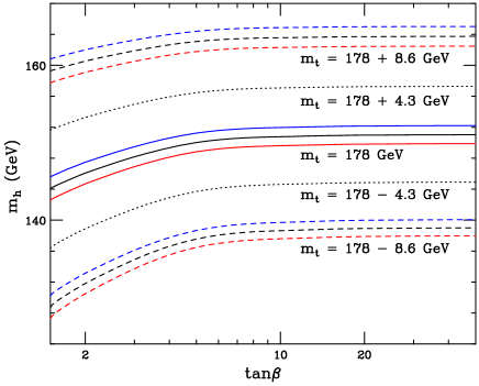
Figure 4: The predicted Higgs mass for the SM with $k_{Y}=4/3$. The red (lower) curves are for $\alpha_{3}+\delta\alpha_{3}$, the blue (upper) $\alpha_{3}-\delta\alpha_{3}$, and the black $\alpha_{3}$. The dotted curves are for $m_{t}\pm\delta m_{t}$, the dash ones for $m_{t}\pm 2\delta m_{t}$, and the solid ones for $m_{t}$.

Furthermore, for the SM with $k_{Y}=$ 5/4 and 32/25, the gauge coupling unifications at two loop are similar to, but not as good as, that of the SM with $k_{Y}=4/3$. Following the same procedure as above, the Higgs mass ranges for $k_{Y}=$ 5/4 and 32/25 turn out to be again from $127$ GeV to $165$ GeV for the $2\sigma$ range of the top quark mass and $1\sigma$ range of $\alpha_{3}$. The Higgs mass ranges corresponding to the more precise (projected) top quark mass $m_{t}=178\pm 1$ GeV are still between $141$ GeV and $154$ GeV.

III 7D Orbifold GUTs

In string model building, orbifold GUTs and their deconstruction, and 4D GUTs with product gauge groups, the normalization for the $U(1)_{Y}$ need not be canonical. As explicit examples, we construct the 7D $SU(6)$ model with $k_{Y}=4/3$ and the 7D $SU(7)$ models with $k_{Y}=5/4$ and 32/25 on the space-time $M^{4}\times T^{2}/Z_{6}\times S^{1}/Z_{2}$ where charge quantization can be realized simultaneously. We also briefly discuss the 7D orbifold $SU(8)$ model with $k_{Y}=7/4$ and charge quantization, and comment on a non-canonical $U(1)_{Y}$ normalization due to the brane localized gauge kinetic terms in orbifold GUTs.

III.1 Gauge Symmetry Breaking on $T^{2}/Z_{6}\times S^{1}/Z_{2}$ Orbifold

The 7D orbifold gauge symmetry breakings have not been studied previously, so we discuss them in detail here. The orbifold gauge symmetry breakings on the 7D space-time $M^{4}\times(S^{1}/Z_{2})^{3}$ are similar to those on the 6-dimensional (6D) space-time $M^{4}\times(S^{1}/Z_{2})^{2}$ Orbifold . Thus, we consider the 7D space-time $M^{4}\times T^{2}/Z_{6}\times S^{1}/Z_{2}$, with coordinates $x^{\mu}$, ($\mu=0,1,2,3$), $x^{5}$, $x^{6}$ and $x^{7}$. Because $T^{2}$ is homeomorphic to $S^{1}\times S^{1}$, we assume that the radii for the circles along the $x^{5}$, $x^{6}$ and $x^{7}$ directions are $R_{1}$, $R_{2}$, and $R^{\prime}$, respectively. For simplicity, we define a complex coordinate $z$ for $T^{2}$ and a real coordinate $y$ for $S^{1}$

$$z\equiv{1\over 2}\left(x^{5}+ix^{6}\right)~{},~{}y\equiv x^{7}~{}.~{}\,$$ (10)

In the complex coordinate, the torus $T^{2}$ can be defined by $C^{1}$ moduloing the equivalent classes:

$$z\sim z+\pi R_{1}~{},~{}z\sim z+\pi R_{2}e^{{\rm i}\theta}~{}.~{}\,$$ (11)

To define the $T^{2}/Z_{6}$ orbifold, we require that $R_{1}=R_{2}\equiv R$ and $\theta=\pi/3$. The $T^{2}/Z_{6}\times S^{1}/Z_{2}$ orbifold is obtained from $T^{2}\times S^{1}$ by moduloing the equivalent classes

$$\Gamma_{T}:~{}~{}z\sim\omega z~{};~{}~{}~{}~{}~{}\Gamma_{S}:~{}~{}y\sim-y~{},~{}\,$$ (12)

where $\omega=e^{{\rm i}\pi/3}$. The fixed points under the $Z_{6}\times Z_{2}$ symmetry are $(z,y)=(0,0)$ and $(0,\pi R^{\prime})$.

Note that our convention is as follows. Suppose $G$ is a Lie group and $H$ is a subgroup of $G$. We denote the commutant of $H$ in $G$ as $\{G/H\}$, i. e.,

$$\{G/H\}\equiv\{g\in G|gh=hg,~{}{\rm for~{}any}~{}h\in H\}~{}.~{}\,$$ (13)

The ${\cal N}=1$ supersymmetry in 7 dimensions has 16 supercharges and corresponds to a ${\cal N}=4$ supersymmetry in 4 dimensions; thus, only the gauge multiplet can be introduced in the bulk. This multiplet can be decomposed under the 4D ${\cal N}=1$ supersymmetry into a vector multiplet $V$ and three chiral multiplets $\Sigma_{1}$, $\Sigma_{2}$, and $\Sigma_{3}$ in the adjoint representation, where the fifth and sixth components of the gauge field, $A_{5}$ and $A_{6}$, are contained in the lowest component of $\Sigma_{1}$, and the seventh component of the gauge field $A_{7}$ is contained in the lowest component of $\Sigma_{2}$. The SM fermions can be on the 3-branes at the $Z_{6}\times Z_{2}$ fixed points, or on the 4-branes at the $Z_{6}$ fixed points.

For the bulk gauge group $G$, we write down the bulk action in the Wess-Zumino gauge and 4D ${\cal N}=1$ supersymmetry language NMASWS ; NAHGW

$${\cal S} = \int d^{7}x\Biggl{\{}{\rm Tr}\Biggl{[}\int d^{2}\theta\left(\frac{1}{4kg^{2}}{\cal W}^{\alpha}{\cal W}_{\alpha}+\frac{1}{kg^{2}}\left(\Sigma_{3}\partial_{z}\Sigma_{2}+\Sigma_{1}\partial_{y}\Sigma_{3}-\frac{1}{\sqrt{2}}\Sigma_{1}[\Sigma_{2},\Sigma_{3}]\right)\right)$$ (14)

$$+{\rm H.C.}\Biggr{]}+\int d^{4}\theta\frac{1}{kg^{2}}{\rm Tr}\Biggl{[}(\sqrt{2}\partial_{z}^{\dagger}+\Sigma_{1}^{\dagger})e^{-V}(-\sqrt{2}\partial_{z}+\Sigma_{1})e^{V}+\partial_{z}^{\dagger}e^{-V}\partial_{z}e^{V}$$

$$+(\sqrt{2}\partial_{y}+\Sigma_{2}^{\dagger})e^{-V}(-\sqrt{2}\partial_{y}+\Sigma_{2})e^{V}+\partial_{y}e^{-V}\partial_{y}e^{V}+{\Sigma_{3}}^{\dagger}e^{-V}\Sigma_{3}e^{V}\Biggr{]}\Biggr{\}}~{}.~{}\,$$

From the above action, we obtain the transformations of the 4D vector multiplet and chiral multiplets

$$V(x^{\mu},~{}\omega z,~{}\omega^{-1}{\bar{z}},~{}y) = R_{\Gamma_{T}}V(x^{\mu},~{}z,~{}{\bar{z}},~{}y)R_{\Gamma_{T}}^{-1}~{},~{}\,$$ (15)

$$\Sigma_{1}(x^{\mu},~{}\omega z,~{}\omega^{-1}{\bar{z}},~{}y) = \omega^{-1}R_{\Gamma_{T}}\Sigma_{1}(x^{\mu},~{}z,~{}{\bar{z}},~{}y)R_{\Gamma_{T}}^{-1}~{},~{}\,$$ (16)

$$\Sigma_{2}(x^{\mu},~{}\omega z,~{}\omega^{-1}{\bar{z}},~{}y) = R_{\Gamma_{T}}\Sigma_{2}(x^{\mu},~{}z,~{}{\bar{z}},~{}y)R_{\Gamma_{T}}^{-1}~{},~{}\,$$ (17)

$$\Sigma_{3}(x^{\mu},~{}\omega z,~{}\omega^{-1}{\bar{z}},~{}y) = \omega R_{\Gamma_{T}}\Sigma_{3}(x^{\mu},~{}z,~{}{\bar{z}},~{}y)R_{\Gamma_{T}}^{-1}~{},~{}\,$$ (18)

$$V(x^{\mu},~{}z,~{}{\bar{z}},~{}-y) = R_{\Gamma_{S}}V(x^{\mu},~{}z,~{}{\bar{z}},~{}y)R_{\Gamma_{S}}^{-1}~{},~{}\,$$ (19)

$$\Sigma_{1}(x^{\mu},~{}z,~{}{\bar{z}},~{}-y) = R_{\Gamma_{S}}\Sigma_{1}(x^{\mu},~{}z,~{}{\bar{z}},~{}y)R_{\Gamma_{S}}^{-1}~{},~{}\,$$ (20)

$$\Sigma_{2}(x^{\mu},~{}z,~{}{\bar{z}},~{}-y) = -R_{\Gamma_{S}}\Sigma_{2}(x^{\mu},~{}z,~{}{\bar{z}},~{}y)R_{\Gamma_{S}}^{-1}~{},~{}\,$$ (21)

$$\Sigma_{3}(x^{\mu},~{}z,~{}{\bar{z}},~{}-y) = -R_{\Gamma_{S}}\Sigma_{3}(x^{\mu},~{}z,~{}{\bar{z}},~{}y)R_{\Gamma_{S}}^{-1}~{}.~{}\,$$ (22)

Here we introduced non-trivial $R_{\Gamma_{T}}$ and $R_{\Gamma_{S}}$ to break the bulk gauge group $G$.

III.2 $SU(6)$ Model with $k_{Y}=4/3$

First, let us consider the $SU(6)$ model, which has $k_{Y}=4/3$. To break the $SU(6)$ gauge symmetry, we choose the following $6\times 6$ matrix representations for $R_{\Gamma_{T}}$ and $R_{\Gamma_{S}}$

$$R_{\Gamma_{T}} = {\rm diag}\left(+1,+1,+1,\omega^{n_{1}},\omega^{n_{1}},\omega^{n_{2}}\right)~{},~{}\,$$ (23)

$$R_{\Gamma_{S}} = {\rm diag}\left(+1,+1,+1,+1,+1,-1\right)~{},~{}\,$$ (24)

where $n_{1}$ and $n_{2}$ are positive integers, and $n_{1}\not=n_{2}$. Then, we obtain

$$\{SU(6)/R_{\Gamma_{T}}\}~{}=~{}SU(3)_{C}\times SU(2)_{L}\times U(1)_{Y}\times U(1)^{\prime}~{},~{}\,$$ (25)

$$\{SU(6)/R_{\Gamma_{S}}\}~{}=~{}SU(5)\times U(1)~{},~{}\,$$ (26)

$$\{SU(6)/\{R_{\Gamma_{T}}\cup R_{\Gamma_{S}}\}\}~{}=~{}SU(3)_{C}\times SU(2)_{L}\times U(1)_{Y}\times U(1)^{\prime}~{}.~{}\,$$ (27)

Therefore, for the zero modes, the 7D ${\cal N}=1$ supersymmetric $SU(6)$ gauge symmetry is broken down to the 4D ${\cal N}=1$ supersymmetric $SU(3)_{C}\times SU(2)_{L}\times U(1)_{Y}\times U(1)^{\prime}$ Li:2001tx .

We define the generators for the $U(1)_{Y}$ and $U(1)^{\prime}$ in the $SU(6)$ as

$$T_{U(1)_{Y}} \equiv {\rm diag}\left({1\over 3},{1\over 3},{1\over 3},-{1\over 3},-{1\over 3},-{1\over 3}\right)~{},~{}\,$$ (28)

$$T_{U(1)^{\prime}} \equiv {\rm diag}\left(0,0,0,{1\over 2},{1\over 2},-1\right)~{},~{}\,$$ (29)

Because ${\rm tr}[T_{U(1)_{Y}}^{2}]=2/3$, we obtain $k_{Y}=4/3$.

The $SU(6)$ adjoint representation $\mathbf{35}$ is decomposed under the $SU(3)_{C}\times SU(2)_{L}\times U(1)_{Y}\times U(1)^{\prime}$ gauge symmetry as

$$\mathbf{35}=\left(\begin{array}[]{ccc}\mathbf{(8,1)}_{Q00}&\mathbf{(3,\bar{2})}_{Q12}&\mathbf{(3,1)}_{Q13}\\ \mathbf{(\bar{3},2)}_{Q21}&\mathbf{(1,3)}_{Q00}&\mathbf{(1,2)}_{Q23}\\ \mathbf{(\bar{3},1)}_{Q31}&\mathbf{(1,\bar{2})}_{Q32}&\mathbf{(1,1)}_{Q00}\end{array}\right)+\mathbf{(1,1)}_{Q00}~{},~{}\,$$ (30)

where the $\mathbf{(1,1)}_{Q00}$ in the third diagonal entry of the matrix and the last term $\mathbf{(1,1)}_{Q00}$ denote the gauge fields for the $U(1)_{Y}\times U(1)^{\prime}$ gauge symmetry. Moreover, the subscripts $Qij$, which are anti-symmetric ($Qij=-Qji$), are the charges under the $U(1)_{Y}\times U(1)^{\prime}$ gauge symmetry

$$Q00~{}=~{}(\mathbf{0},\mathbf{0})~{},~{}Q12=(\mathbf{2\over 3},\mathbf{-{1\over 2}})~{},~{}Q13=(\mathbf{2\over 3},\mathbf{1})~{},~{}Q23~{}=~{}(\mathbf{0},\mathbf{3\over 2})~{}.~{}\,$$ (31)

The $Z_{6}\times Z_{2}$ transformation properties for the decomposed components of $V$, $\Sigma_{1}$, $\Sigma_{2}$, and $\Sigma_{3}$ are

$$V:\left(\begin{array}[]{ccc}(1,+)&(\omega^{-n_{1}},+)&(\omega^{-n_{2}},-)\\ (\omega^{n_{1}},+)&(1,+)&(\omega^{n_{1}-n_{2}},-)\\ (\omega^{n_{2}},-)&(\omega^{n_{2}-n_{1}},-)&(1,+)\end{array}\right)+(1,+)~{},~{}\,$$ (32)

$$\Sigma_{1}:\left(\begin{array}[]{ccc}(\omega^{-1},+)&(\omega^{-n_{1}-1},+)&(\omega^{-n_{2}-1},-)\\ (\omega^{n_{1}-1},+)&(\omega^{-1},+)&(\omega^{n_{1}-n_{2}-1},-)\\ (\omega^{n_{2}-1},-)&(\omega^{n_{2}-n_{1}-1},-)&(\omega^{-1},+)\end{array}\right)+(\omega^{-1},+)~{},~{}\,$$ (33)

$$\Sigma_{2}:\left(\begin{array}[]{ccc}(1,-)&(\omega^{-n_{1}},-)&(\omega^{-n_{2}},+)\\ (\omega^{n_{1}},-)&(1,-)&(\omega^{n_{1}-n_{2}},+)\\ (\omega^{n_{2}},+)&(\omega^{n_{2}-n_{1}},+)&(1,-)\end{array}\right)+(1,-)~{},~{}\,$$ (34)

$$\Sigma_{3}:\left(\begin{array}[]{ccc}(\omega,-)&(\omega^{-n_{1}+1},-)&(\omega^{-n_{2}+1},+)\\ (\omega^{n_{1}+1},-)&(\omega,-)&(\omega^{n_{1}-n_{2}+1},+)\\ (\omega^{n_{2}+1},+)&(\omega^{n_{2}-n_{1}+1},+)&(\omega,-)\end{array}\right)+(\omega,-)~{},~{}\,$$ (35)

where the zero modes transform as $(1,+)$. We choose

$$n_{1}~{}=~{}2~{},~{}~{}n_{2}~{}=~{}5~{}.~{}\,$$ (36)

From Eqs. (32)-(35), we obtain that, for the zero modes, the 7D ${\cal N}=1$ supersymmetric $SU(6)$ gauge symmetry is broken down to the 4D ${\cal N}=1$ supersymmetric $SU(3)_{C}\times SU(2)_{L}\times U(1)_{Y}\times U(1)^{\prime}$ gauge symmetry. Also, we have no zero modes from chiral multiplets $\Sigma_{1}$ and $\Sigma_{2}$, and we have one and only one zero mode from $\Sigma_{3}$ with quantum number $\mathbf{(\bar{3},1)}_{Q31}$ under the $SU(3)_{C}\times SU(2)_{L}\times U(1)_{Y}\times U(1)^{\prime}$ gauge symmetry, which can be considered as the right-handed top quark because its hypercharge is $\mathbf{-2/3}$.

On the 3-brane at the $Z_{6}\times Z_{2}$ fixed point $(z,y)=(0,0)$, the preserved gauge symmetry is $SU(3)_{C}\times SU(2)_{L}\times U(1)_{Y}\times U(1)^{\prime}$ Li:2001tx . Thus, on the observable 3-brane at $(z,y)=(0,0)$, we can introduce one pair of Higgs doublets and three families of the SM quarks and leptons except the right-handed top quark. Because the $U(1)_{Y}$ charge for the right-handed top quark is determined from the construction, charge quantization can be achieved from the anomaly free conditions and the gauge invariance of the Yukawa couplings on the observable 3-brane. Moreover, the $U(1)^{\prime}$ anomalies can be cancelled by assigning suitable $U(1)^{\prime}$ charges to the SM quarks and leptons, for example, we assign the $U(1)^{\prime}$ charges for the first, second and third families of the SM fermions as $\mathbf{+1}$, $\mathbf{0}$, $\mathbf{-1}$, respectively. Also, the $U(1)^{\prime}$ gauge symmetry can be broken at the GUT scale by introducing one pair of SM singlets with $U(1)^{\prime}$ charges $\mathbf{\pm 1}$ on the observable 3-brane. Interestingly, this $U(1)^{\prime}$ gauge symmetry may be considered as a flavour symmetry, and then the SM fermion masses and mixings may be explained naturally via the Froggatt-Nielsen mechanism FN . Furthermore, supersymmetry can be broken around the compactification scale, which can be considered as the GUT scale, for example, by the Scherk–Schwarz mechanism Scherk:1978ta .

III.3 $SU(7)$ Models with $k_{Y}=5/4$ and $32/25$

We will construct the $SU(7)$ models with $k_{Y}=5/4$ and $32/25$. Because these two models are quite similar, we discuss them simultaneously.

To break the $SU(7)$ gauge symmetry, we choose the following $7\times 7$ matrix representations for $R_{\Gamma_{T}}$ and $R_{\Gamma_{S}}$

$$R_{\Gamma_{T}} = {\rm diag}\left(+1,+1,+1,\omega^{n_{1}},\omega^{n_{1}},\omega^{n_{1}},\omega^{n_{2}}\right)~{},~{}\,$$ (37)

$$R_{\Gamma_{S}} = {\rm diag}\left(+1,+1,+1,+1,+1,-1,-1\right)~{},~{}\,$$ (38)

where $n_{1}$ and $n_{2}$ are positive integers, and $n_{1}\not=n_{2}$. Then, we obtain

$$\{SU(7)/R_{\Gamma_{T}}\}~{}=~{}SU(3)_{C}\times SU(3)\times U(1)\times U(1)^{\prime}~{},~{}\,$$ (39)

$$\{SU(7)/R_{\Gamma_{S}}\}~{}=~{}SU(5)\times SU(2)\times U(1)~{},~{}\,$$ (40)

$$\{SU(7)/\{R_{\Gamma_{T}}\cup R_{\Gamma_{S}}\}\}~{}=~{}SU(3)_{C}\times SU(2)_{L}\times U(1)_{Y}\times U(1)_{\alpha}\times U(1)_{\beta}~{}.~{}\,$$ (41)

Therefore, we obtain that, for the zero modes, the 7D ${\cal N}=1$ supersymmetric $SU(7)$ gauge symmetry is broken down to the 4D ${\cal N}=1$ supersymmetric $SU(3)_{C}\times SU(2)_{L}\times U(1)_{Y}\times U(1)_{\alpha}\times U(1)_{\beta}$ gauge symmetry Li:2001tx .

The $SU(7)$ adjoint representation $\mathbf{48}$ is decomposed under the $SU(3)_{C}\times SU(2)_{L}\times U(1)_{Y}\times U(1)_{\alpha}\times U(1)_{\beta}$ gauge symmetry as

$$\mathbf{48}=\left(\begin{array}[]{cccc}\mathbf{(8,1)}_{Q00}&\mathbf{(3,\bar{2})}_{Q12}&\mathbf{(3,1)}_{Q13}&\mathbf{(3,1)}_{Q14}\\ \mathbf{(\bar{3},2)}_{Q21}&\mathbf{(1,3)}_{Q00}&\mathbf{(1,2)}_{Q23}&\mathbf{(1,2)}_{Q24}\\ \mathbf{(\bar{3},1)}_{Q31}&\mathbf{(1,\bar{2})}_{Q32}&\mathbf{(1,1)}_{Q00}&\mathbf{(1,1)}_{Q34}\\ \mathbf{(\bar{3},1)}_{Q41}&\mathbf{(1,\bar{2})}_{Q42}&\mathbf{(1,1)}_{Q43}&\mathbf{(1,1)}_{Q00}\end{array}\right)+\mathbf{(1,1)}_{Q00}~{},~{}\,$$ (42)

where the $\mathbf{(1,1)}_{Q00}$ in the third and fourth diagonal entries of the matrix and the last term $\mathbf{(1,1)}_{Q00}$ denote the gauge fields for the $U(1)_{Y}\times U(1)_{\alpha}\times U(1)_{\beta}$ gauge symmetry. Moreover, the subscripts $Qij$, which are anti-symmetric ($Qij=-Qji$), are the charges under the $U(1)_{Y}\times U(1)_{\alpha}\times U(1)_{\beta}$ gauge symmetry. The subscript $Q00~{}=~{}(\mathbf{0},\mathbf{0},\mathbf{0})$, and the other subscripts $Qij$ with $i\not=j$ will be given for each model explicitly.

(1) $SU(7)$ model with $k_{Y}=5/4$. We define the generators for the $U(1)_{Y}\times U(1)_{\alpha}\times U(1)_{\beta}$ gauge symmetry as follows

$$T_{U(1)_{Y}} \equiv {\rm diag}\left({1\over 4},{1\over 4},{1\over 4},-{1\over 4},-{1\over 4},{1\over 4},-{1\over 2}\right)~{},~{}\,$$ (43)

$$T_{U(1)_{\alpha}} \equiv {\rm diag}\left(1,1,1,-3,-3,-1,4\right)~{},~{}\,$$ (44)

$$T_{U(1)_{\beta}} \equiv {\rm diag}\left(-{8\over 9},-{8\over 9},-{8\over 9},-{1\over 2},-{1\over 2},3,{2\over 3}\right)~{}.~{}\,$$ (45)

Because ${\rm tr}[T_{U(1)_{Y}}^{2}]=5/8$, we obtain $k_{Y}=5/4$. In this paper, we will choose convenient generators (normalizations) for $U(1)_{\alpha}\times U(1)_{\beta}$ gauge symmetry.

The $U(1)_{Y}\times U(1)_{\alpha}\times U(1)_{\beta}$ charges $Qij$ are

$$Q12=(\mathbf{1\over 2},\mathbf{4},\mathbf{-{7\over{18}}})~{},~{}Q13=(\mathbf{0},\mathbf{2},\mathbf{-{{35}\over{9}}})~{},~{}Q14=(\mathbf{3\over 4},\mathbf{-3},\mathbf{-{{14}\over{9}}})~{},~{}\,$$ (46)

$$Q23=(\mathbf{-{1\over 2}},\mathbf{-2},\mathbf{-{7\over{2}}})~{},~{}Q24=(\mathbf{{1\over 4}},\mathbf{-7},\mathbf{-{7\over{6}}})~{},~{}Q34=(\mathbf{{3\over 4}},\mathbf{-5},\mathbf{{7\over{3}}})~{}.~{}\,$$ (47)

(2) $SU(7)$ model with $k_{Y}=32/25$. We define the generators for the $U(1)_{Y}\times U(1)_{\alpha}\times U(1)_{\beta}$ gauge symmetry as follows

$$T_{U(1)_{Y}} \equiv {\rm diag}\left({3\over{10}},{3\over{10}},{3\over{10}},-{2\over 5},-{2\over 5},{1\over{10}},-{1\over 5}\right)~{},~{}\,$$ (48)

$$T_{U(1)_{\alpha}} \equiv {\rm diag}\left(1,1,1,3,3,-1,-8\right)~{},~{}\,$$ (49)

$$T_{U(1)_{\beta}} \equiv {\rm diag}\left(-47,-47,-47,-12,-12,219,-54\right)~{}.~{}\,$$ (50)

Because ${\rm tr}[T_{U(1)_{Y}}^{2}]=16/25$, we obtain $k_{Y}=32/25$.

The $U(1)_{Y}\times U(1)_{\alpha}\times U(1)_{\beta}$ charges $Qij$ are

$$Q12=(\mathbf{7\over{10}},\mathbf{-2},\mathbf{-35})~{},~{}Q13=(\mathbf{1\over 5},\mathbf{2},\mathbf{-266})~{},~{}Q14=(\mathbf{1\over 2},\mathbf{9},\mathbf{7})~{},~{}\,$$ (51)

$$Q23=(\mathbf{-{1\over 2}},\mathbf{4},\mathbf{-231})~{},~{}Q24=(\mathbf{-{1\over 5}},\mathbf{11},\mathbf{42})~{},~{}Q34=(\mathbf{{3\over{10}}},\mathbf{7},\mathbf{273})~{}.~{}\,$$ (52)

The $Z_{6}\times Z_{2}$ transformation properties for the decomposed components of $V$, $\Sigma_{1}$, $\Sigma_{2}$, and $\Sigma_{3}$ are

$$V:\left(\begin{array}[]{cccc}(1,+)&(\omega^{-n_{1}},+)&(\omega^{-n_{1}},-)&(\omega^{-n_{2}},-)\\ (\omega^{n_{1}},+)&(1,+)&(1,-)&(\omega^{n_{1}-n_{2}},-)\\ (\omega^{n_{1}},-)&(1,-)&(1,+)&(\omega^{n_{1}-n_{2}},+)\\ (\omega^{n_{2}},-)&(\omega^{n_{2}-n_{1}},-)&(\omega^{n_{2}-n_{1}},+)&(1,+)\end{array}\right)+(1,+)~{},~{}\,$$ (53)

$$\Sigma_{1}:\left(\begin{array}[]{cccc}(\omega^{-1},+)&(\omega^{-n_{1}-1},+)&(\omega^{-n_{1}-1},-)&(\omega^{-n_{2}-1},-)\\ (\omega^{n_{1}-1},+)&(\omega^{-1},+)&(\omega^{-1},-)&(\omega^{n_{1}-n_{2}-1},-)\\ (\omega^{n_{1}-1},-)&(\omega^{-1},-)&(\omega^{-1},+)&(\omega^{n_{1}-n_{2}-1},+)\\ (\omega^{n_{2}-1},-)&(\omega^{n_{2}-n_{1}-1},-)&(\omega^{n_{2}-n_{1}-1},+)&(\omega^{-1},+)\end{array}\right)+(\omega^{-1},+)~{},~{}\,$$ (54)

$$\Sigma_{2}:\left(\begin{array}[]{ccccc}(1,-)&(\omega^{-n_{1}},-)&(\omega^{-n_{1}},+)&(\omega^{-n_{2}},+)\\ (\omega^{n_{1}},-)&(1,-)&(1,+)&(\omega^{n_{1}-n_{2}},+)\\ (\omega^{n_{1}},+)&(1,+)&(1,-)&(\omega^{n_{1}-n_{2}},-)\\ (\omega^{n_{2}},+)&(\omega^{n_{2}-n_{1}},+)&(\omega^{n_{2}-n_{1}},-)&(1,-)\end{array}\right)+(1,-)~{},~{}\,$$ (55)

$$\Sigma_{3}:\left(\begin{array}[]{ccccc}(\omega,-)&(\omega^{-n_{1}+1},-)&(\omega^{-n_{1}+1},+)&(\omega^{-n_{2}+1},+)\\ (\omega^{n_{1}+1},-)&(\omega,-)&(\omega,+)&(\omega^{n_{1}-n_{2}+1},+)\\ (\omega^{n_{1}+1},+)&(\omega,+)&(\omega,-)&(\omega^{n_{1}-n_{2}+1},-)\\ (\omega^{n_{2}+1},+)&(\omega^{n_{2}-n_{1}+1},+)&(\omega^{n_{2}-n_{1}+1},-)&(\omega,-)\end{array}\right)+(\omega,-)~{},~{}\,$$ (56)

where the zero modes transform as $(1,+)$. We choose

$$n_{1}~{}=~{}2~{},~{}~{}n_{2}~{}=~{}4~{}.~{}\,$$ (57)

From Eqs. (53)-(56), we obtain that, for the zero modes, the 7D ${\cal N}=1$ supersymmetric $SU(7)$ gauge symmetry is broken down to the 4D ${\cal N}=1$ supersymmetric $SU(3)_{C}\times SU(2)_{L}\times U(1)_{Y}\times U(1)_{\alpha}\times U(1)_{\beta}$ gauge symmetry. Also, we have no zero modes from chiral multiplets $\Sigma_{1}$ and $\Sigma_{3}$, and we have only one pair of zero modes from $\Sigma_{2}$ with quantum numbers $\mathbf{(1,2)}_{Q23}$ and $\mathbf{(1,\bar{2})}_{Q32}$ under the $SU(3)_{C}\times SU(2)_{L}\times U(1)_{Y}\times U(1)_{\alpha}\times U(1)_{\beta}$ gauge symmetry, which can be considered as one pair of the Higgs doublets $H_{d}$ and $H_{u}$ in the supersymmetric models, respectively.

On the 3-brane at the $(z,y)=(0,0)$, the preserved gauge symmetry is $SU(3)_{C}\times SU(2)_{L}\times U(1)_{Y}\times U(1)_{\alpha}\times U(1)_{\beta}$ Li:2001tx . Thus, on the observable 3-brane at $(z,y)=(0,0)$, we can introduce three families of the SM fermions. Because the $U(1)_{Y}$ hypercharges for one pair of Higgs doublets $H_{d}$ and $H_{u}$ are determined from the model building, charge quantization can be achieved from the anomaly free conditions and the gauge invariance of the Yukawa couplings on the observable 3-brane. Moreover, because $H_{d}$ and $H_{u}$ are vector-like under the $SU(3)_{C}\times SU(2)_{L}\times U(1)_{Y}\times U(1)_{\alpha}\times U(1)_{\beta}$ gauge symmetry, there are no $U(1)_{\alpha}$ and $U(1)_{\beta}$ anomalies from them. The $U(1)_{\alpha}\times U(1)_{\beta}$ gauge symmetry can be broken at the GUT scale by introducing two pairs of the SM singlets with non-trivial $U(1)_{\alpha}\times U(1)_{\beta}$ charges on the observable 3-brane. The remarks at the end of above subsection for the fermion spectrum and supersymmetry breaking apply here as well.

III.4 $SU(8)$ Model with $k_{Y}=7/4$

We briefly present a 7D orbifold $SU(8)$ model with $k_{Y}=7/4$, which gives an alternative $U(1)_{Y}$ normalization for the MSSM. To avoid confusion, we emphasize that in this model we consider TeV-scale supersymmetry breaking. To break the $SU(8)$ gauge symmetry, we choose the following $8\times 8$ matrix representations for $R_{\Gamma_{T}}$ and $R_{\Gamma_{S}}$

$$R_{\Gamma_{T}} = {\rm diag}\left(+1,+1,+1,\omega^{n_{1}},\omega^{n_{1}},\omega^{n_{1}},\omega^{n_{2}},\omega^{n_{2}}\right)~{},~{}\,$$ (58)

$$R_{\Gamma_{S}} = {\rm diag}\left(+1,+1,+1,+1,+1,-1,-1,+1\right)~{},~{}\,$$ (59)

where $n_{1}$ and $n_{2}$ are positive integers, and $n_{1}\not=n_{2}$. Then, we find

$$\{SU(8)/R_{\Gamma_{T}}\}~{}=~{}SU(3)_{C}\times SU(3)\times SU(2)\times U(1)^{2}~{},~{}\,$$ (60)

$$\{SU(8)/R_{\Gamma_{S}}\}~{}=~{}SU(6)\times SU(2)\times U(1)~{},~{}\,$$ (61)

$$\{SU(8)/\{R_{\Gamma_{T}}\cup R_{\Gamma_{S}}\}\}~{}=~{}SU(3)_{C}\times SU(2)_{L}\times U(1)_{Y}\times U(1)_{\alpha}\times U(1)_{\beta}\times U(1)_{\gamma}~{}.~{}\,$$ (62)

Therefore, we obtain that, for the zero modes, the 7D ${\cal N}=1$ supersymmetric $SU(8)$ gauge symmetry is broken down to the 4D ${\cal N}=1$ supersymmetric $SU(3)_{C}\times SU(2)_{L}\times U(1)_{Y}\times U(1)_{\alpha}\times U(1)_{\beta}\times U(1)_{\gamma}$ gauge symmetry Li:2001tx .

We define the $U(1)_{Y}$ generator as following

$$T_{U(1)_{Y}} \equiv {\rm diag}\left({1\over 4},{1\over 4},{1\over 4},{1\over 4},{1\over 4},-{1\over 4},-{1\over 2},-{1\over 2}\right)~{}.~{}\,$$ (63)

Because ${\rm tr}[T_{U(1)_{Y}}^{2}]=7/8$, we obtain $k_{Y}=7/4$. We choose

$$n_{1}~{}=~{}5~{},~{}~{}n_{2}~{}=~{}4~{}.~{}\,$$ (64)

After detailed calculations, we find that there are one pair of Higgs doublets $H_{d}$ and $H_{u}$ from the zero modes of $\Sigma_{2}$ and some exotic particles from the zero modes of the chiral multiplets $\Sigma_{1}$, $\Sigma_{2}$ and $\Sigma_{3}$.

Similar to the above subsection, we introduce three families of SM fermions on the observable 3-brane at $(z,y)=(0,0)$ and charge quantization can be realized. The $U(1)_{\alpha}\times U(1)_{\beta}\times U(1)_{\gamma}$ gauge symmetry can be considered as a flavour symmetry, and it can be broken at the GUT scale by introducing three pairs of the SM singlets with non-trivial $U(1)_{\alpha}\times U(1)_{\beta}\times U(1)_{\gamma}$ charges on the observable 3-brane. In addition, the exotic particles from the zero modes of chiral multiplets $\Sigma_{i}$ can be made very heavy after the $U(1)_{\alpha}\times U(1)_{\beta}\times U(1)_{\gamma}$ gauge symmetry breaking by coupling them to the extra fields on the observable 3-brane.

III.5 Remarks on Another Possibility

In 5-dimensional (5D) orbifold $SU(5)$, or 6D orbifold $SO(10)$ Orbifold , the SM gauge couplings $g_{Y}$, $g_{2}$, and $g_{3}$ at the unification scale are obtained from compactification, i.e.,

$$g_{Y}=g_{Y}^{B}~{},~{}~{}g_{2}=g_{2}^{B}~{},~{}~{}g_{3}=g^{B}_{3}~{},~{}\,$$ (65)

where $g_{Y}^{B}$, $g_{2}^{B}$ and $g^{B}_{3}$ are the properly normalized 4D effective gauge couplings from 5D $SU(5)$ or 6D $SO(10)$ gauge kinetic terms. Because we have ${\sqrt{5\over 3}}g_{Y}^{B}=g_{2}^{B}=g^{B}_{3}$ at the unification scale, we obtain

$${\sqrt{5\over 3}}g_{Y}=g_{2}=g_{3}~{}.~{}\,$$ (66)

However, on the 3-branes at the fixed points, only the SM or SM-like gauge symmetry should be preserved, so there exists the possibility that one may introduce the 3-brane localized gauge kinetic terms from the effective field theory point of view Dvali:2000rx . Thus, the effective SM gauge couplings $g_{Y}$, $g_{2}$, and $g_{3}$ at the unification scale become

$${1\over g_{Y}^{2}}={1\over g_{Y}^{B2}}+{1\over g_{Y}^{\prime 2}}~{},~{}~{}{1\over g_{2}^{2}}={1\over g_{2}^{B2}}+{1\over g_{2}^{\prime 2}}~{},~{}~{}{1\over g_{3}^{2}}={1\over g_{3}^{B2}}+{1\over g_{3}^{\prime 2}}~{},~{}\,$$ (67)

where $g_{Y}^{\prime}$, $g_{2}^{\prime}$ and $g^{\prime}_{3}$ are the properly normalized 4D effective gauge couplings from 3-brane localized gauge kinetic terms. In general, we have

$${\sqrt{5\over 3}}g_{Y}^{\prime}\not=g_{2}^{\prime}\not=g_{3}^{\prime}~{}.~{}\,$$ (68)

Thus, at the unification scale, we obtain

$${\sqrt{5\over 3}}g_{Y}\not=g_{2}\not=g_{3}~{}.~{}\,$$ (69)

Therefore, the $U(1)_{Y}$ (and other gauge factors) normalization is not canonical.

In this paper we just point out this possibility, but we do not take it seriously for these reasons: (1) To achieve the gauge coupling unification in the SM, we need to fine-tune the brane localized gauge kinetic terms; (2) There are no such brane localized gauge kinetic terms in the orbifold compactifications of the weakly coupled heterotic string theory Dixon:1985jw ; thus, whether such terms do exist is unresolved.

IV Discussion and Conclusions

How to test our models with different $U(1)_{Y}$ normalizations is an interesting question. However, it is very difficult for two reasons. First, there exist unkown threshhold corrections (including the supersymmetric threshold corrections) close to the GUT scale because a lot of new particles may appear, and higher-dimensional operators may also contribute to the gauge couplings, so the concrete prediction for one of the three SM gauge couplings at the weak scale due to the RGE running from the unification scale will be GUT model dependent. Furthermore, the RGE running of the gauge couplings in the SM for different $U(1)_{Y}$ normalizations will not cause any physically different results at low energy, i. e., the SM with different $U(1)_{Y}$ normalizations are equivalent as low energy effective theories.

The string landscape suggests that the supersymmetry breaking scale can be high and then the simplest low energy effective theory is just the SM. Considering GUT scale supersymmetry breaking, we showed that gauge coupling unification in the SM can be achieved at about $10^{16-17}$ GeV for $k_{Y}=4/3$, 5/4, 32/25. Especially for $k_{Y}=4/3$, gauge coupling unification in the SM is well satisfied at two loop order. We also predicted that the Higgs mass is in the range 127 GeV to 165 GeV by varying $\alpha_{3}$ within its $1\sigma$ range, $m_{t}$ within its $2\sigma$ range and $\tan\beta$ from $1.5$ to $50$. For a future top quark mass measurement of value and uncertainty $m_{t}=178\pm 1$ GeV, for example, we obtained a Higgs boson mass between $141$ GeV and $154$ GeV. Moreover, we pointed out that gauge coupling unification in the MSSM does not necessarily imply $k_{Y}=5/3$. We showed that gauge coupling unification in the MSSM can be achieved at the same level by choosing $k_{Y}=7/4$.

Furthermore, we constructed a 7D $SU(6)$ model with $k_{Y}=4/3$ and 7D $SU(7)$ models with $k_{Y}=5/4$ and 32/25 on the space-time $M^{4}\times T^{2}/Z_{6}\times S^{1}/Z_{2}$. In these models, the $SU(6)$ and $SU(7)$ gauge symmetries can be broken down to the SM-like gauge symmetries via orbifold projections and then broken further down to the SM gauge symmetry by the Higgs mechanism. The right-handed top quark in the $SU(6)$ model and one pair of the Higgs doublets in the $SU(7)$ models can be obtained from the zero modes of the bulk vector multiplet, with their hypercharges determined by the constructions. Then charge quantization can be achieved from the anomaly free conditions and the gauge invariance of the Yukawa couplings. The extra $U(1)$ gauge symmetries can be considered as flavour symmetries, and then the SM fermion masses and mixings may be explained naturally via the Froggatt-Nielsen mechanism FN . The supersymmetry can be broken at the GUT scale by the Scherk–Schwarz mechanism Scherk:1978ta . We also briefly presented a 7D orbifold $SU(8)$ model with $k_{Y}=7/4$ and charge quantization and commented on non-canonical $U(1)_{Y}$ normalization due to the brane localized gauge kinetic terms in orbifold GUTs.

Appendix A Renormalization Group Equations

In this Appendix, following our convention in Ref. Barger:2004sf , we give the renormalization group equations in the SM and supersymmetric models with a general normalization factor $k_{Y}$. The general formulae for the renormalization group equations in the SM are given in Refs. mac ; Cvetic:1998uw , and those for the supersymmetric models are given in Refs. Barger:1992ac ; Barger:1993gh ; Martin:1993zk .

First, we present the renormalization group equations in the SM. The two-loop renormalization group equations for the gauge couplings are

$$(4\pi)^{2}\frac{d}{dt}~{}g_{i}=g_{i}^{3}b_{i}+\frac{g_{i}^{3}}{(4\pi)^{2}}\left[\sum_{j=1}^{3}B_{ij}g_{j}^{2}-\sum_{\alpha=u,d,e}d_{i}^{\alpha}{\rm Tr}\left(h^{\alpha\dagger}h^{\alpha}\right)\right]~{},~{}\,$$ (70)

The beta-function coefficients are

$$b=\left(\frac{41}{6}\frac{1}{k_{Y}},-\frac{19}{6},-7\right)~{},~{}B=\pmatrix{\frac{199}{18}\frac{1}{k_{Y}^{2}}&\frac{27}{6}\frac{1}{k_{Y}}&\frac{44}{3}\frac{1}{k_{Y}}\cr\frac{3}{2}\frac{1}{k_{Y}}&\frac{35}{6}&12\cr\frac{11}{6}\frac{1}{k_{Y}}&\frac{9}{2}&-26}~{},~{}$$ (71)

$$d^{u}=\left(\frac{17}{6}\frac{1}{k_{Y}},\frac{3}{2},2\right)~{},~{}d^{d}=\left(\frac{5}{6}\frac{1}{k_{Y}},\frac{3}{2},2\right)~{},~{}d^{e}=\left(\frac{5}{2}\frac{1}{k_{Y}},\frac{1}{2},0\right)~{}.~{}\,$$ (72)

Since the contributions in Eq. (70) from the Yukawa couplings arise from two-loop diagrams, we only need to include Yukawa coupling evolution at one-loop order. The one-loop renormalization group equations for Yukawa couplings are

$$(4\pi)^{2}\frac{d}{dt}~{}h^{u} = h^{u}\left(-\sum_{i=1}^{3}c_{i}^{u}g_{i}^{2}+\frac{3}{2}h^{u\dagger}h^{u}-\frac{3}{2}h^{d\dagger}h^{d}+\Delta_{2}\right)~{},~{}$$ (73)

$$(4\pi)^{2}\frac{d}{dt}~{}h^{d} = h^{d}\left(-\sum_{i=1}^{3}c_{i}^{d}g_{i}^{2}-\frac{3}{2}h^{u\dagger}h^{u}+\frac{3}{2}h^{d\dagger}h^{d}+\Delta_{2}\right)~{},~{}$$ (74)

$$(4\pi)^{2}\frac{d}{dt}~{}h^{e} = h^{e}\left(-\sum_{i=1}^{3}c_{i}^{e}g_{i}^{2}+\frac{3}{2}h^{e\dagger}h^{e}+\Delta_{2}\right)~{},~{}\,$$ (75)

where

$$c^{u}=\left(\frac{17}{12}\frac{1}{k_{Y}},\frac{9}{4},8\right)~{},~{}c^{d}=\left(\frac{5}{12}\frac{1}{k_{Y}},\frac{9}{4},8\right)~{},~{}c^{e}=\left(\frac{15}{4}\frac{1}{k_{Y}},\frac{9}{4},0\right)~{},~{}$$ (76)

$$\Delta_{2} = {\rm Tr}(3h^{u\dagger}h^{u}+3h^{d\dagger}h^{d}+h^{e\dagger}h^{e})~{}.~{}$$ (77)

The one-loop renormalization group equation for the Higgs quartic coupling is

$$(4\pi)^{2}\frac{d}{dt}~{}\lambda = 12\lambda^{2}-\left(3\frac{1}{k_{Y}}g_{1}^{2}+9g_{2}^{2}\right)\lambda+{9\over 4}\left(\frac{1}{3}\frac{1}{k_{Y}^{2}}g_{1}^{4}+{2\over 3}\frac{1}{k_{Y}}g_{1}^{2}g_{2}^{2}+g_{2}^{4}\right)$$ (78)

$$+4\Delta_{2}\lambda-4\Delta_{4}~{},~{}\,$$

where

$$\Delta_{4} = {\rm Tr}\left[3(h^{u\dagger}h^{u})^{2}+3(h^{d\dagger}h^{d})^{2}+(h^{e\dagger}h^{e})^{2}\right]~{}.~{}$$ (79)

Second, we give the beta-function coefficients for supersymmetric models. The two-loop renormalization group equations for the gauge couplings are the same as Eq. (70). The beta-function coefficients are modified due to the new particle contents. They are

$$b=\left(11\frac{1}{k_{Y}},1,-3\right)~{},~{}B=\pmatrix{\frac{199}{9}\frac{1}{k_{Y}^{2}}&9\frac{1}{k_{Y}}&\frac{88}{3}\frac{1}{k_{Y}}\cr 3\frac{1}{k_{Y}}&25&24\cr\frac{11}{3}\frac{1}{k_{Y}}&9&14}~{},~{}$$ (80)

$$d^{u}=\left(\frac{26}{3}\frac{1}{k_{Y}},6,4\right)~{},~{}d^{d}=\left(\frac{14}{3}\frac{1}{k_{Y}},6,4\right)~{},~{}d^{e}=\left(6\frac{1}{k_{Y}},2,0\right)~{}.~{}$$ (81)

The one-loop renormalization group equations for Yukawa couplings are

$$(4\pi)^{2}\frac{d}{dt}~{}y^{u} = y^{u}\left[3y^{u\dagger}y^{u}+y^{d\dagger}y^{d}+3{\rm Tr}(y^{u\dagger}y^{u})-\sum_{i=1}^{3}c_{i}^{u}g_{i}^{2}\right]~{},~{}$$ (82)

$$(4\pi)^{2}\frac{d}{dt}~{}y^{d} = y^{d}\left[y^{u\dagger}y^{u}+3y^{d\dagger}y^{d}+{\rm Tr}(3y^{d\dagger}y^{d}+y^{e\dagger}y^{e})-\sum_{i=1}^{3}c_{i}^{d}g_{i}^{2}\right]~{},~{}$$ (83)

$$(4\pi)^{2}\frac{d}{dt}~{}y^{e} = y^{e}\left[3y^{e\dagger}y^{e}+{\rm Tr}(3y^{d\dagger}y^{d}+y^{e\dagger}y^{e})-\sum_{i=1}^{3}c_{i}^{e}g_{i}^{2}\right]~{},~{}$$ (84)

where

$$c^{u}=\left(\frac{13}{9}\frac{1}{k_{Y}},3,\frac{16}{3}\right)~{},~{}c^{d}=\left(\frac{7}{9}\frac{1}{k_{Y}},3,\frac{16}{3}\right)~{},~{}c^{e}=\left(3\frac{1}{k_{Y}},3,0\right)~{}.~{}$$ (86)

References

- (1) R. Bousso and J. Polchinski, JHEP 0006, 006 (2000); S. B. Giddings, S. Kachru and J. Polchinski, Phys. Rev. D 66, 106006 (2002); S. Kachru, R. Kallosh, A. Linde and S. P. Trivedi, Phys. Rev. D 68, 046005 (2003); L. Susskind, arXiv:hep-th/0302219; F. Denef and M. R. Douglas, arXiv:hep-th/0404116; F. Denef and M. R. Douglas, arXiv:hep-th/0411183.
- (2) S. Weinberg, Phys. Rev. Lett. 59 (1987) 2607.
- (3) A. Giryavets, S. Kachru and P. K. Tripathy, JHEP 0408 (2004) 002; L. Susskind, arXiv:hep-th/0405189; M. R. Douglas, arXiv:hep-th/0405279; arXiv:hep-th/0409207; M. Dine, E. Gorbatov and S. Thomas, arXiv:hep-th/0407043; E. Silverstein, arXiv:hep-th/0407202; J. P. Conlon and F. Quevedo, arXiv:hep-th/0409215; M. Dine, D. O’Neil and Z. Sun, arXiv:hep-th/0501214.
- (4) N. Arkani-Hamed and S. Dimopoulos, arXiv:hep-th/0405159.
- (5) V. Barger, C. W. Chiang, J. Jiang and T. Li, Nucl. Phys. B 705, 71 (2005).
- (6) A. Arvanitaki, C. Davis, P. W. Graham and J. G. Wacker, Phys. Rev. D 70, 117703 (2004); G. F. Giudice and A. Romanino, Nucl. Phys. B 699, 65 (2004) [Erratum-ibid. B 706, 65 (2005)]; A. Pierce, Phys. Rev. D 70, 075006 (2004); C. Kokorelis, arXiv:hep-th/0406258; S. Profumo and C. E. Yaguna, Phys. Rev. D 70, 095004 (2004); S. H. Zhu, Phys. Lett. B 604, 207 (2004); P. H. Chankowski, A. Falkowski, S. Pokorski and J. Wagner, Phys. Lett. B 598, 252 (2004).
- (7) W. Kilian, T. Plehn, P. Richardson and E. Schmidt, Eur. Phys. J. C 39, 229 (2005); R. Mahbubani, arXiv:hep-ph/0408096; M. Binger, arXiv:hep-ph/0408240; J. L. Hewett, B. Lillie, M. Masip and T. G. Rizzo, JHEP 0409, 070 (2004); L. Anchordoqui, H. Goldberg and C. Nunez, arXiv:hep-ph/0408284; S. K. Gupta, P. Konar and B. Mukhopadhyaya, Phys. Lett. B 606, 384 (2005); K. Cheung and W. Y. Keung, Phys. Rev. D 71, 015015 (2005); N. Arkani-Hamed, S. Dimopoulos, G. F. Giudice and A. Romanino, Nucl. Phys. B 709, 3 (2005).
- (8) D. A. Demir, arXiv:hep-ph/0410056; U. Sarkar, arXiv:hep-ph/0410104; R. Allahverdi, A. Jokinen and A. Mazumdar, Phys. Rev. D 71, 043505 (2005); E. J. Chun and S. C. Park, JHEP 0501, 009 (2005); I. Antoniadis and S. Dimopoulos, arXiv:hep-th/0411032; B. Bajc and G. Senjanovic, arXiv:hep-ph/0411193; B. Kors and P. Nath, arXiv:hep-th/0411201; A. Arvanitaki and P. W. Graham, arXiv:hep-ph/0411376.
- (9) A. Masiero, S. Profumo and P. Ullio, arXiv:hep-ph/0412058; M. A. Diaz and P. F. Perez, arXiv:hep-ph/0412066; L. Senatore, arXiv:hep-ph/0412103; K. R. Dienes, E. Dudas and T. Gherghetta, arXiv:hep-th/0412185; A. Datta and X. Zhang, arXiv:hep-ph/0412255; P. C. Schuster, arXiv:hep-ph/0412263; S. P. Martin, K. Tobe and J. D. Wells, arXiv:hep-ph/0412424.
- (10) C. H. Chen and C. Q. Geng, arXiv:hep-ph/0501001; K. S. Babu, T. Enkhbat and B. Mukhopadhyaya, arXiv:hep-ph/0501079; N. Arkani-Hamed, S. Dimopoulos and S. Kachru, arXiv:hep-th/0501082. M. Drees, arXiv:hep-ph/0501106; S. Kasuya and F. Takahashi, arXiv:hep-ph/0501240; K. Cheung and C. W. Chiang, arXiv:hep-ph/0501265; K. Huitu, J. Laamanen, P. Roy and S. Roy, arXiv:hep-ph/0502052; N. Haba and N. Okada, arXiv:hep-ph/0502213; C. H. Chen and C. Q. Geng, arXiv:hep-ph/0502246.
- (11) B. Dutta and Y. Mimura, arXiv:hep-ph/0503052; D. Chang, W. F. Chang and W. Y. Keung, arXiv:hep-ph/0503055; N. G. Deshpande and J. Jiang, arXiv:hep-ph/0503116; A. Ibarra, arXiv:hep-ph/0503160; B. Mukhopadhyaya and S. SenGupta, arXiv:hep-ph/0503167; M. Toharia and J. D. Wells, arXiv:hep-ph/0503175; B. Thomas, arXiv:hep-ph/0503248.
- (12) J. F. Donoghue, Phys. Rev. D 69, 106012 (2004) [Erratum-ibid. D 69, 129901 (2004)].
- (13) For reviews see: J. E. Kim, Phys. Rep. 150 (1987) 1; H. Y. Cheng, Phys. Rep. 158 (1988) 1; M. S. Turner, Phys. Rep. 197 (1991) 67; G. G. Raffelt, Phys. Rep. 333 (2000) 593; G. Gabadadze and M. Shifman, Int. J. Mod. Phys. A17 (2002) 3689.
- (14) Particle Data Group, K. Hagiwara et al, Phys. Rev. D66 (2002) 010001-173.
- (15) P. G. Camara, L. E. Ibanez and A. M. Uranga, Nucl. Phys. B 708, 268 (2005); G. L. Kane, P. Kumar, J. D. Lykken and T. T. Wang, arXiv:hep-ph/0411125; A. Font and L. E. Ibanez, arXiv:hep-th/0412150.
- (16) R. D. Peccei and H. R. Quinn, Phys. Rev. Lett. 38 (1977) 1440; Phys. Rev. D16 (1977) 1791.
- (17) K. S. Babu, I. Gogoladze and K. Wang, Phys. Lett. B 560, 214 (2003).
- (18) M. B. Green and J. H. Schwarz, Phys. Lett. B149 (1984) 117; Nucl. Phys. B255 (1985) 93; M. B. Green, J. H. Schwarz and P. West, Nucl. Phys. B254 (1985) 327.
- (19) V. Barger, J. Jiang, P. Langacker and T. Li, arXiv:hep-ph/0503226.
- (20) H. Davoudiasl, R. Kitano, T. Li and H. Murayama, arXiv:hep-ph/0405097.
- (21) C. D. Froggatt and H. B. Nielsen, Nucl. Phys. B147 (1979) 277.
- (22) P. Langacker and M. X. Luo, Phys. Rev. D 44, 817 (1991); J. R. Ellis, S. Kelley and D. V. Nanopoulos, Phys. Lett. B 260, 131 (1991); U. Amaldi, W. de Boer and H. Furstenau, Phys. Lett. B 260, 447 (1991).
- (23) P. H. Frampton and S. L. Glashow, Phys. Lett. B 131, 340 (1983) [Erratum-ibid. B 135, 515 (1984)]. S. Nandi, Phys. Lett. B 142, 375 (1984); H. Murayama and T. Yanagida, Mod. Phys. Lett. A 7, 147 (1992); T. G. Rizzo, Phys. Rev. D 45, 3903 (1992).
- (24) X. Calmet, arXiv:hep-ph/0406314.
- (25) K. R. Dienes, Phys. Rept. 287, 447 (1997).
- (26) R. Blumenhagen, M. Cvetic, P. Langacker and G. Shiu, arXiv:hep-th/0502005.
- (27) Y. Kawamura, Prog. Theor. Phys. 103, 613 (2000); G. Altarelli and F. Feruglio, Phys. Lett. B 511, 257 (2001); L. Hall and Y. Nomura, Phys. Rev. D 64, 055003 (2001); A. Hebecker and J. March-Russell, Nucl. Phys. B 613, 3 (2001); T. Li, Phys. Lett. B 520, 377 (2001); Nucl. Phys. B 619, 75 (2001); T. Asaka, W. Buchmuller and L. Covi, Phys. Lett. B 523, 199 (2001); I. Gogoladze, Y. Mimura and S. Nandi, Phys. Rev. Lett. 91, 141801 (2003).
- (28) T. Li, Nucl. Phys. B 633, 83 (2002).
- (29) N. Arkani-Hamed, A. G. Cohen and H. Georgi, Phys. Rev. Lett. 86, 4757 (2001); C. T. Hill, S. Pokorski and J. Wang, Phys. Rev. D 64, 105005 (2001); C. Csaki, G. D. Kribs and J. Terning, Phys. Rev. D 65, 015004 (2002); H. C. Cheng, K. T. Matchev and J. Wang, Phys. Lett. B 521, 308 (2001); T. Li and T. Liu, Eur. Phys. J. C 28, 545 (2003); C. S. Huang, J. Jiang and T. Li, Nucl. Phys. B 702, 109 (2004).
- (30) M. Beneke et al., arXiv:hep-ph/0003033.
- (31) J. Scherk and J. H. Schwarz, Phys. Lett. B 82, 60 (1979).
- (32) P. Azzi et al. [CDF and D0 Collaborations], arXiv:hep-ex/0404010.
- (33) S. Bethke, arXiv:hep-ex/0407021.
- (34) S. Eidelman et al. [Particle Data Group Collaboration], Phys. Lett. B 592, 1 (2004).
- (35) P. Langacker and N. Polonsky, Phys. Rev. D 47, 4028 (1993); Phys. Rev. D 52, 3081 (1995); M. Carena, S. Pokorski and C. E. M. Wagner, Nucl. Phys. B 406, 59 (1993).
- (36) M. E. Machacek and M. T. Vaughn, Nucl. Phys. B 222, 83 (1983); Nucl. Phys. B 236, 221 (1984); Nucl. Phys. B 249, 70 (1985).
- (37) G. Cvetic, C. S. Kim and S. S. Hwang, Phys. Rev. D 58, 116003 (1998).
- (38) V. D. Barger, M. S. Berger and P. Ohmann, Phys. Rev. D 47, 1093 (1993).
- (39) V. D. Barger, M. S. Berger and P. Ohmann, Phys. Rev. D 49, 4908 (1994).
- (40) S. P. Martin and M. T. Vaughn, Phys. Rev. D 50, 2282 (1994), and references therein.
- (41) H. Arason, D. J. Castano, B. Keszthelyi, S. Mikaelian, E. J. Piard, P. Ramond and B. D. Wright, Phys. Rev. D 46, 3945 (1992); H. E. Haber, R. Hempfling and A. H. Hoang, Z. Phys. C 75, 539 (1997).
- (42) N. Marcus, A. Sagnotti and W. Siegel, Nucl. Phys. B 224, 159 (1983).
- (43) N. Arkani-Hamed, T. Gregoire and J. Wacker, hep-th/0101233.
- (44) G. R. Dvali, G. Gabadadze and M. A. Shifman, Phys. Lett. B 497, 271 (2001); H. Georgi, A. K. Grant and G. Hailu, Phys. Lett. B 506, 207 (2001).
- (45) L. J. Dixon, J. A. Harvey, C. Vafa and E. Witten, Nucl. Phys. B 261, 678 (1985); Nucl. Phys. B 274, 285 (1986).