New cosmological mass limit on thermal relic axions

Abstract

Observations of the cosmological large-scale structure provide well-established neutrino mass limits. We extend this argument to thermal relic axions. We calculate the axion thermal freeze-out temperature and thus their cosmological abundance on the basis of their interaction with pions. For hadronic axions we find a new mass limit $m_{a}<1.05$ eV (95% CL), corresponding to a limit on the axion decay constant of $f_{a}>5.7\times 10^{6}$ GeV. For other models this constraint is significantly weakened only if the axion-pion coupling is strongly suppressed. For comparison we note that the same approach leads to $\sum m_{\nu}<0.65$ eV (95% CL) for neutrinos.

1 Introduction

Low-mass cosmic relic particles provide a hot-dark matter component of the universe. After they decouple in the early universe, they freely stream and decrease the spectral power of primordial density fluctuations on small scales. This well-studied effect has been established as a standard method to derive neutrino mass limits where the results of different authors differ primarily in the used observational data sets and assumed priors on some of the cosmological parameters (for a recent review see Ref. [1]). Two of us have recently extended this method to several generic cases of other low-mass thermal relics that may have been produced in the early universe [2], for example weakly interacting bosons such as the hypothetical axions.

For a generic low-mass particle species $X$ that was once in thermal equilibrium, the crucial parameters that enter the structure-formation argument are the assumed particle mass $m_{X}$, the number $g_{X}$ of internal degrees of freedom, the relevant quantum statistics (boson vs. fermion), and finally the number $g_{*}$ of effective cosmic thermal degrees of freedom at the epoch when the $X$ particles thermally decouple. These parameters imply the present-day cosmic mass density $\Omega_{X}$ in these particles as well as their velocity distribution and primordial free-streaming scale.

In Ref. [2] two of us considered thermal relic axions as a specific example and found an upper mass limit of 2–3 eV. The main purpose of the present paper is to sharpen this result in two ways. First, we use an updated set of observational data. Second, we take a closer look at the axion freeze-out in the early universe to obtain a more accurate value for $g_{*}$ in terms of the appropriate coupling constants.

We begin in Sec. 2 with a brief summary of the relevant aspects of axion physics and continue in Sec. 3 with a determination of the freeze-out conditions as a function of the relevant axion coupling constants. In Sec. 4 we perform a likelihood analysis based on recent cosmological data to determine the allowed range of axion parameters. We finish in Sec. 5 with a summary and interpretation of our results.

2 Axions

Quantum chromodynamics is a CP-violating theory, implying that the neutron should have a large electric dipole moment, in conflict with the opposite experimental evidence. The most elegant solution of this “strong CP problem” was proposed by Peccei and Quinn (PQ) who showed that CP conservation is dynamically restored in the presence of a new global U(1) symmetry that is spontaneously broken at some large energy scale [3, 4]. Weinberg [5] and Wilczek [6] realized that an inevitable consequence of the PQ mechanism is the existence of a new pseudoscalar boson, the axion, which is the Nambu-Goldstone boson of the PQ symmetry. This symmetry is explicitly broken at low energies by instanton effects so that the axion acquires a small mass. Unless there are non-QCD contributions, perhaps from Planck-scale physics [7, 8], the mass is

$$m_{a}=\frac{z^{1/2}}{1+z}\,\frac{f_{\pi}m_{\pi}}{f_{a}}=\frac{6.0~{}{\rm eV}}{f_{a}/10^{6}~{}{\rm GeV}}\,,$$ (1)

where the energy scale $f_{a}$ is the axion decay constant or PQ scale that governs all axion properties, $f_{\pi}=93$ MeV is the pion decay constant, and $z=m_{u}/m_{d}$ is the mass ratio of the up and down quarks. We will follow the previous axion literature and assume a value $z=0.56$ [9, 10], but we note that it could vary in the range 0.3–0.7 [11].

The PQ scale is constrained by various experiments and astrophysical arguments that involve processes where axions interact with photons, electrons, and hadrons. The interaction strength with these particles scales as $f_{a}^{-1}$, apart from model-dependent numerical factors. If axions indeed exist, experimental and astrophysical limits suggest that $f_{a}\,\hbox to0.0pt{\lower 3.7pt\hbox{$\mathchar 0\relax\sim$}\hss}\raise 1.0pt\hbox{$>$}\,0.6\times 10^{9}$ GeV and $m_{a}\,\hbox to0.0pt{\lower 3.7pt\hbox{$\mathchar 0\relax\sim$}\hss}\raise 1.0pt\hbox{$<$}\,0.01$ eV [12, 11].

Perhaps the most robust limits are those on the axion interaction strength with photons and electrons because the properties of ordinary stars can be used to test anomalous energy losses caused by processes such as $\gamma+e^{-}\to e^{-}+a$ or the Primakoff process $\gamma+Ze\to Ze+a$ [12, 11]. These limits are so restrictive that processes involving the electron and photon couplings will not be significant for the thermalization of axions in the early universe in the post-QCD epoch. On the other hand, these interactions are also the most model dependent. Axion-models can be constructed where the axion-photon interaction is arbitrarily small. In “hadronic axion models” such as the KSVZ model [13, 14] there is no tree-level interaction with ordinary quarks and leptons, and in any case, the axion-electron coupling can be very small even in non-hadronic models such as the DFSZ model [15, 16]. Therefore, the restrictive stellar limits on the electron and photon couplings do not conclusively rule out axions with a PQ scale in the $10^{6}$ GeV range that is of interest to us.

The axion-nucleon interaction strength is constrained by two different limits based on the observed neutrino signal of supernova 1987A [12, 11]. The axionic energy loss caused by processes such as $NN\to NNa$ excludes a window of the axion-nucleon interaction strength where the axionic contribution to the loss or transfer of energy would have been comparable to or larger than that of neutrinos. For a sufficiently large interaction strength, axions no longer compete with neutrinos for the overall energy transfer in the supernova core, but then would cause too many events in the water Cherenkov detectors that observed the neutrino signal. However, there is a narrow intermediate range of couplings, corresponding to $f_{a}$ around $10^{6}$ GeV, i.e. to an axion mass of a few eV, where neither argument is conclusive. In this “hadronic axion window,” these elusive particles may still be allowed. This observation has previously led to the speculation that axions with eV-masses could contribute a significant hot dark-matter fraction to the universe [17].

Assuming that axions do not couple to charged leptons, the main thermalization processes in the post-QCD epoch involve hadrons [18]

$$a+\pi\leftrightarrow\pi+\pi\,,$$ (2)

$$a+N\leftrightarrow N+\pi\,.$$ (3)

Due to the scarcity of nucleons relative to pions, the pionic processes are actually by far the most important. Therefore, we need the axion-pion interaction which is given by a Lagrangian of the form [18]

$${\cal L}_{a\pi}=\frac{C_{a\pi}}{f_{\pi}f_{a}}\,\left(\pi^{0}\pi^{+}\partial_{\mu}\pi^{-}+\pi^{0}\pi^{-}\partial_{\mu}\pi^{+}-2\pi^{+}\pi^{-}\partial_{\mu}\pi^{0}\right)\partial_{\mu}a\,.$$ (4)

In hadronic axion models where the ordinary quarks and leptons do not carry PQ charges, the coupling constant is [18]

$$C_{a\pi}=\frac{1-z}{3\,(1+z)}\,.$$ (5)

In non-hadronic models an additional term enters that could, in principle, reduce $C_{a\pi}$. For the DFSZ model, the relevant $a$-$\pi^{0}$-mixing strength was derived by Carena and Peccei [19]. In the DFSZ model, however, axions in our $f_{a}$ range are already excluded so that we mainly focus on hadronic models.

3 Axion decoupling

3.1 Pionic process

Axions are an often-cited cold dark matter candidate if they interact so weakly (if $f_{a}$ is so large) that they never achieve thermal equilibrium [23, 24, 25, 26, 27]. In that case coherent oscillations of the axion field are excited around the QCD transition when the PQ symmetry is explicitly broken by instanton effects. However, if $f_{a}$ is sufficiently small so that axions interact sufficiently strongly, they will thermalize and survive as thermal relics in analogy to neutrinos [18, 20, 21]. In the eV-range of axion masses that is of interest to us, thermalization will happen after the QCD transition so that one has to consider axion interactions with hadrons rather than interactions with quarks and gluons that would be relevant at earlier epochs.

Axions freeze out when their rate of interaction becomes slow compared to the cosmic expansion rate. As a criterion for axion thermal decoupling we use

$$\langle\Gamma_{a}\rangle_{T}=H(T)\,,$$ (6)

where $\langle\Gamma_{a}\rangle_{T}$ is the axion absorption rate, averaged over a thermal distribution at temperature $T$, whereas $H(T)$ is the Hubble expansion parameter at the cosmic temperature $T$. Our freeze-out criterion is accurate up to a constant of order unity. In principle, the full system of Boltzmann equations should be followed for all species, but the use of $H(T)=\langle\Gamma_{a}\rangle_{T}$ only introduces an error of 10–20% in the decoupling temperature, consistent with the other approximations we will use.

As explained in Sec. 2, by far the most important process for axion thermalization is the pionic reaction of Eq. (2) which is of the form $1+2\to 3+4$ with particle 1 the axion and particles 2–4 the pions. The average absorption rate is

$$\langle\Gamma_{a}\rangle_{T} = \frac{1}{n_{a}}\int\frac{d^{3}{\bf p}_{1}}{(2\pi)^{3}2E_{1}}\,\frac{d^{3}{\bf p}_{2}}{(2\pi)^{3}2E_{2}}\,\frac{d^{3}{\bf p}_{3}}{(2\pi)^{3}2E_{3}}\,\frac{d^{3}{\bf p}_{4}}{(2\pi)^{3}2E_{4}}\,\sum|{\cal M}|^{2}$$ (7)

$$\hskip 20.00003pt{}\times(2\pi)^{4}\,\delta^{4}(p_{1}+p_{2}-p_{3}-p_{4})\,f_{1}f_{2}(1+f_{3})(1+f_{4})\,,$$

where $f_{j}$ are the thermal occupation numbers. The axion number density in thermal equilibrium is $n_{a}=\int d^{3}{\bf p}_{1}f_{1}/(2\pi)^{3}=(\zeta_{3}/\pi^{2})\,T^{3}$.

The interaction Eq. (4) implies the three pionic processes $a+\pi^{0}\to\pi^{+}+\pi^{-}$, $a+\pi^{+}\to\pi^{+}+\pi^{0}$, and $a+\pi^{-}\to\pi^{-}+\pi^{0}$. Assuming equal mass $m_{\pi}$ for both charged and neutral pions, we find for the squared matrix element, summed over all three channels,

$$\sum|{\cal M}|^{2}=\frac{9}{4}\,\left(\frac{C_{a\pi}}{f_{a}f_{\pi}}\right)^{2}\left(s^{2}+t^{2}+u^{2}-3m_{\pi}^{4}\right)\,,$$ (8)

where $s=(p_{1}+p_{2})^{2}$, $t=(p_{1}-p_{3})^{2}$, and $u=(p_{1}-p_{4})^{2}$.

We have performed the phase-space integration in Eq. (7) along the lines of the method described in Ref. [22]. Chang and Choi [18] give an explicit three-dimensional integral expression for the average rate of $\pi\pi\to\pi a$ when the final-state stimulation factors $(1+f_{3})(1+f_{4})$ are neglected. Our numerical integration agrees with their result if we consider the same quantity, but in the following we use our full expression for the average absorption rate. From dimensional considerations one finds

$$\langle\Gamma_{a}\rangle_{T}=A\,\left(\frac{C_{a\pi}}{f_{a}f_{\pi}}\right)^{2}\,T^{5}\,h(m_{\pi}/T)\,,$$ (9)

where numerically $A=0.215$. The function $h(\mu)$ is normalized to $h(0)=1$ (Fig. 1).

• 

Figure 1: Dimensionless axion absorption rate $h(\mu)$ as defined by Eq. (9).

3.2 Expansion rate

The cosmic expansion rate is given by the Friedmann equation as $H^{2}=8\pi G_{\rm N}\rho/3$ with $G_{\rm N}$ the Newton constant and $\rho$ the mass-energy density. For the radiation dominated epoch one usually writes [28]

$$\rho=\frac{\pi^{2}}{30}\,g_{*}(T)\,T^{4}=\sum_{j={\rm particles}}g_{j}\int\frac{d^{3}{\bf p}}{(2\pi)^{3}}\frac{(m_{j}^{2}+{\bf p}^{2})^{1/2}}{\exp\left[(m_{j}^{2}+{\bf p}^{2})^{1/2}/T\right]\pm 1}$$ (10)

where $g_{*}(T)$ denotes the effective number of thermal degrees of freedom that are excited at the epoch with temperature $T$. Further, $g_{j}$ is the number of internal degrees of freedom of a given particle species $j$ with mass $m_{j}$. The $\pm 1$ in the denominator applies to bosons and fermions, respectively. We assume vanishing chemical potentials for all particles. For the conditions of interest, the particle-antiparticle asymmetry is small even for nucleons. The Friedmann equation is thus

$$H=\left[\frac{4\pi^{3}}{45}\,g_{*}(T)\right]^{1/2}\,\frac{T^{2}}{m_{\rm Pl}}\,,$$ (11)

where $m_{\rm Pl}=G_{\rm N}^{-1/2}$ is the Planck mass.

We consider all particles with masses up to the nucleon mass as listed in Table 1. In the upper panel of Fig. 2 we show the function $g_{*}(T)$, assuming that only the particles of Table 1 contribute and ignoring the color deconfinement transition that probably takes place at a temperature somewhat below 200 MeV.

Table 1: Particles that contribute to $g_{*}$ during the post-QCD epoch

• Particles	Mass [MeV]	Spin	$g_{j}$
  $\gamma$	0	$1$	2
  $\nu$, $\bar{\nu}$	0	$\frac{1}{2}$	6
  $e^{\pm}$	0.511	$\frac{1}{2}$	4
  $\mu^{\pm}$	106	$\frac{1}{2}$	4
  $\pi^{0}$, $\pi^{\pm}$	138	$0$	3
  $K^{0}$, $\bar{K}^{0}$, $K^{\pm}$	494	$0$	4
  $\eta$	547	$0$	1
  $\rho^{0}$, $\rho^{\pm}$	771	1	9
  $\omega$	782	$1$	3
  $K^{*0}$, $\bar{K}^{*0}$, $K^{*\pm}$	892	$1$	12
  $n$, $p$, $\bar{n}$, $\bar{p}$	938	$\frac{1}{2}$	8

• 
• 

Figure 2: Effective number of thermal degrees of freedom in the early universe during the post-QCD epoch, assuming the particle content listed in Table 1. Upper panel: $g_{*}$. Lower Panel: $g_{*S}/g_{*}$.

The effective number of thermal degrees of freedom $g_{*}$ that appears in the Friedmann equation is the quantity that governs the expansion rate. However, if axions freeze out at a certain epoch, their number density at late times is governed by $g_{*S}$, the effective number of thermal degrees characterizing the entropy at the freeze-out epoch. The entropy density of an ideal gas is given by the general expression $(\rho+P)/T\propto g_{*S}T^{3}$ with $P$ the pressure. The pressure is given by the same integral expression as the energy density in Eq. (10) after replacing $E_{j}=(m_{j}^{2}+{\bf p}^{2})^{1/2}$ by $\frac{1}{3}\,{\bf p}\cdot{\bf v}=\frac{1}{3}{\bf p}^{2}/E_{j}$. Even though we assume that all particles are in thermal equilibrium at the same temperature, there will be a difference between $g_{*}$ and $g_{*S}$ because some of the contributing particles are not massless. In the lower panel of Fig. 2 we show the ratio $g_{*S}/g_{*}$. Since the deviation of $g_{*}$ from $g_{*S}$ is at most a few percent for the conditions of interest, we will henceforth ignore the difference between the two quantities and always use $g_{*}$. Moreover, since axions themselves contribute only a single degree of freedom we neglect their contribution to $g_{*}$ for simplicity.

3.3 Freeze-out conditions

We now combine our result for the cosmic expansion rate in the post-QCD epoch with that for the axion absorption rate and determine the freeze-out conditions from Eq. (6). As an example we show $H(T)$ and $\langle\Gamma_{a}\rangle_{T}$ in Fig. 3, assuming a PQ scale of $f_{a}=10^{7}$ GeV and the hadronic axion-pion coupling of Eq. (5). From the intersection point we determine $T_{\rm D}$, the axion decoupling temperature, and the corresponding $g_{*}$. We show these quantities as functions of $f_{a}$ in Fig. 4 and in Table 2.

Moreover, from $g_{*}$ at decoupling one can determine the present-day number density of axions by virtue of the relation

$$n_{a}=\frac{g_{*S}({\rm today})}{g_{*S}({\rm decoupling})}\times\,\frac{n_{\gamma}}{2}\,,$$ (12)

where $n_{\gamma}=411~{}{\rm cm}^{-3}$ [11] is the present-day density of cosmic microwave photons and today $g_{*S}=3.91$ [28]. We show $n_{a}$ as a function of $f_{a}$ in Fig. 4 and give some numerical values in Table 2. For comparison, we note that the present-day neutrino number density, determined by standard neutrino freeze-out, is $n_{\nu}\simeq 112~{}{\rm cm}^{-3}$.

• 

Figure 3: Average axion absorption rate for $f_{a}=10^{7}$ GeV and cosmic expansion rate as a function of the cosmic temperature. Rates are in units of $T^{2}/m_{\rm Pl}$.

• 
• 
• 

Figure 4: Axion freeze-out, assuming the $a$-$\pi$ coupling of Eq. (5). Top: Decoupling temperature. Middle: Corresponding $g_{*}$. Bottom: Present-day axion density.

Table 2: Thermal decoupling conditions for axions, assuming the hadronic axion-pion coupling of Eq. (5). $n_{a}$ is the expected present-day axion density.

• $f_{a}$ [GeV]	$T_{\rm D}$ [MeV]	$g_{*}(T_{\rm D})$	$n_{a}$ [cm-3]
  $3\times 10^{3}$	13.37	10.84	74.14
  $1\times 10^{4}$	15.30	10.93	73.50
  $3\times 10^{4}$	17.63	11.10	72.39
  $1\times 10^{5}$	21.21	11.46	70.11
  $3\times 10^{5}$	26.06	12.06	66.63
  $1\times 10^{6}$	34.75	13.15	61.08
  $3\times 10^{6}$	49.12	14.54	55.24
  $1\times 10^{7}$	81.61	16.43	48.88
  $3\times 10^{7}$	145.31	21.10	38.08

4 Likelihood analysis

4.1 Theoretical predictions

In order to derive limits on the axion parameters we compare theoretical power spectra for the matter distribution and the CMB temperature fluctuations with observational data in analogy to previous works by one of us [29, 30, 31]. The predicted power spectra are calculated with the publicly available CMBFAST package [32]. As in our previous paper on general low-mass thermal relics [2] we have modified the code to include a scalar boson that decouples earlier than neutrinos, i.e. we assume a number density and velocity distribution according to the freeze-out epoch.

As a set of cosmological parameters apart from the axion characteristics we choose the matter density $\Omega_{\rm M}$, the baryon density $\Omega_{\rm B}$, the Hubble parameter $H_{0}$, the scalar spectral index of the primordial fluctuation spectrum $n_{s}$, the optical depth to reionization $\tau$, the normalization of the CMB power spectrum $Q$, and the bias parameter $b$. We restrict our analysis to geometrically flat models $\Omega=\Omega_{\rm M}+\Omega_{\Lambda}=1$. The cosmological parameters and their assumed priors are listed in Table 3. The actual marginalization over parameters was performed using a simulated annealing procedure [33]. The cosmological parameters in our model corresponds to the simplest $\Lambda$CDM model which fits present data. While our results would be changed slightly by including additional parameters, there would be no significant changes [2].

Likelihoods are calculated from $\chi^{2}$ so that for 1 parameter estimates, 68% confidence regions are determined by $\Delta\chi^{2}=\chi^{2}-\chi_{0}^{2}=1$, and 95% regions by $\Delta\chi^{2}=4$. Here, $\chi_{0}^{2}$ refers to the best-fit model.

Table 3: Priors on cosmological parameters used in the likelihood analysis.

• Parameter	Prior	Distribution
  $\Omega=\Omega_{\rm M}+\Omega_{\Lambda}$	1	Fixed
  $\Omega_{\rm M}$	0.1–1	Top Hat
  $h$	$0.72\pm 0.08$	Gaussian
  $\Omega_{\rm B}h^{2}$	0.014–0.040	Top hat
  $n_{s}$	0.6–1.4	Top hat
  $\tau$	0–1	Top hat
  $Q$	—	Free
  $b$	—	Free

4.2 Cosmological Data

4.2.1 Large Scale Structure.

At present there are two large galaxy surveys of comparable size, the Sloan Digital Sky Survey (SDSS) [35, 34] and the 2 degree Field Galaxy Redshift Survey (2dFGRS) [36]. Once the SDSS is completed it will be significantly larger and more accurate than the 2dFGRS. We will only use data from SDSS, but the results would be almost identical with 2dFGRS data. We use only data on scales larger than $k=0.15\,h~{}{\rm Mpc}^{-1}$ to avoid problems with non-linearity.

4.2.2 Cosmic Microwave Background.

The CMB temperature fluctuations are conveniently described in terms of the spherical harmonics power spectrum $C_{l}^{TT}\equiv\langle|a_{lm}|^{2}\rangle$, where $\frac{\Delta T}{T}(\theta,\phi)=\sum_{lm}a_{lm}Y_{lm}(\theta,\phi)$. Since Thomson scattering polarizes light, there are also power spectra coming from the polarization. The polarization can be divided into a curl-free $(E)$ and a curl $(B)$ component, yielding four independent power spectra: $C_{l}^{TT}$, $C_{l}^{EE}$, $C_{l}^{BB}$, and the $T$-$E$ cross-correlation $C_{l}^{TE}$.

The WMAP experiment has reported data only on $C_{l}^{TT}$ and $C_{l}^{TE}$ as described in Refs. [37, 38, 39, 40, 41]. We have performed our likelihood analysis using the prescription given by the WMAP collaboration [38, 39, 40, 41] which includes the correlation between different $C_{l}$’s. Foreground contamination has already been subtracted from their published data.

4.2.3 Supernova luminosity distances.

We use the “gold” data set compiled and described by Riess et al. [42] consisting of 157 SNe Ia using a modified version of the SNOC package [43].

4.2.4 The Lyman-$\alpha$ forest.

We have furthermore used the Lyman-$\alpha$ forest data from Croft et al. [44]. The error bars on the last three data points have been increased in the same fashion as was done by the WMAP collaboration [37, 38, 39, 40, 41], in order to make them compatible with the analysis of Gnedin and Hamilton [45]. While there is some controversy about the use of Lyman-$\alpha$ data for parameter estimation it should be noted that their inclusion has only a very small quantitative effect on our results as will become clear below.

4.2.5 Hubble parameter.

Additionally we use data on the Hubble parameter from the HST key project [46], $h=H_{0}/(100~{}{\rm km}~{}{\rm s}^{-1}~{}{\rm Mpc}^{-1})=0.72\pm 0.08$.

4.3 Limits on axion parameters

After marginalizing over the cosmological parameters shown in Table 3, the 68% and 95% CL allowed regions of axion parameters are shown in Fig. 5. In the upper panel we have included the full data set described above, while in the lower panel we have removed the Lyman-$\alpha$ data that is perhaps our most uncertain input.

The Lyman-$\alpha$ data only has a significant impact for high values of $g_{*}$ because it measures very small scales. The large-scale structure data loses sensitivity at $k\,\hbox to0.0pt{\lower 3.7pt\hbox{$\mathchar 0\relax\sim$}\hss}\raise 1.0pt\hbox{$<$}\,0.15\,h~{}{\rm Mpc}^{-1}$, whereas the Lyman-$\alpha$ data probes scales which are about an order of magnitude smaller. For high $g_{*}$, the particle mass for a given value of $\Omega_{a}h^{2}$ is higher and therefore the free-streaming length is correspondingly smaller. The change in power spectrum amplitude occurs at $k>0.15\,h~{}{\rm Mpc}^{-1}$ and is only measurable in the Lyman-$\alpha$ data when $g_{*}\,\hbox to0.0pt{\lower 3.7pt\hbox{$\mathchar 0\relax\sim$}\hss}\raise 1.0pt\hbox{$>$}\,60$–70.

• 
• 

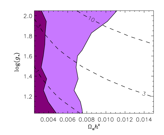
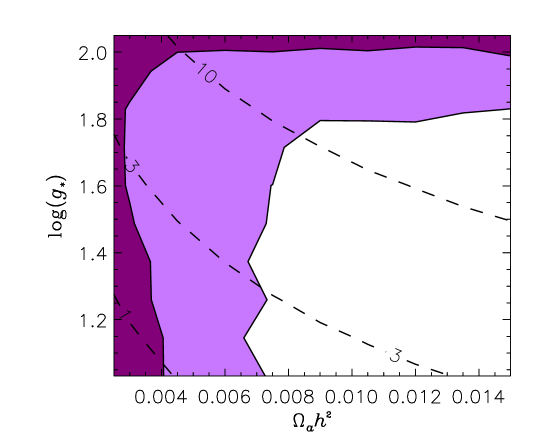
Figure 5: Likelihood contours for the allowed axion parameters. Everything to the right of the dark shaded region is excluded at the 68% CL, and everything to the right of the light shaded region is excluded at the 95% CL. Contours of equal axion mass with the indicated $m_{a}$ values in eV are shown as dashed lines. Upper panel: All data included. Lower panel: Lyman-$\alpha$ data excluded.

In Fig. 6 we show the same analysis as in the upper panel of Fig. 5, but now transformed to the $m_{a}$-$g_{*}$-plane. The hadronic axion model is shown as a thick solid line. It lies at relatively small values of $g_{*}$ for the relevant mass range, meaning that there will be very little quantitative difference if the Lyman-$\alpha$ data is not used.

• 

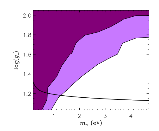
Figure 6: Likelihood contours including all data, equivalent to the upper panel of Fig. 5, transformed to the parameter plane of $g_{*}$ and $m_{a}$. The relation between $g_{*}$ and $m_{a}$ for hadronic axions is shown as a thick solid line.

• 

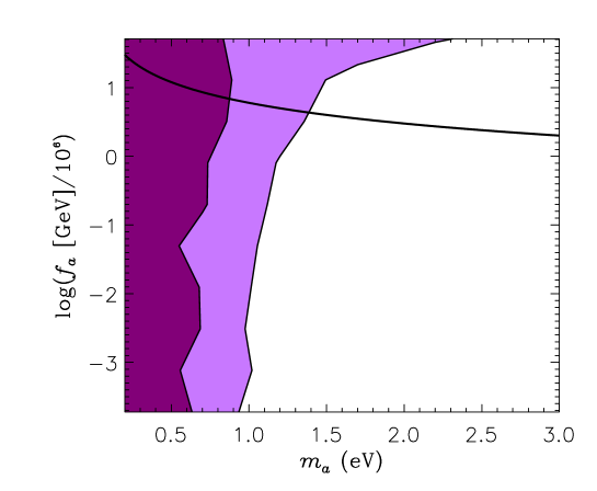
Figure 7: Likelihood contours including all data, equivalent to the upper panel of Fig. 5, transformed to the parameter plane of $f_{a}$ and $m_{a}$. We have used the connection between $g_{*}$ and $f_{a}$ for hadronic axions as shown in Fig. 4 and Table 2. The standard $m_{a}$-$f_{a}$-relation of Eq. (1) is shown as a thick solid line.

Likewise, in Fig. 7 we show the analysis in the $m_{a}$-$f_{a}$-plane, where the relationship between $f_{a}$ and $g_{*}$ shown in Fig. 4 and Table 2 has been used. In this figure, the true independent variable on the vertical axis is the axion-pion coupling that was transformed to a value for the PQ scale assuming the hadronic case Eq. (5). For other models with different $C_{a\pi}$, the vertical axis in Fig. 7 must be re-scaled accordingly. Moreover, the standard relationship between $m_{a}$ and $f_{a}$ of Eq. (1) and the hadronic axion-pion coupling of Eq. (5) put axions on the thick solid line.

In this case, where the most specific assumptions about the underlying axion model were made, the axion parameter space collapses to one dimension, leading to a more restrictive mass limit. In Fig. 8 we show a one-dimensional likelihood analysis for this case, i.e. for the hadronic axion model. As a result one finds a 95% CL excluded region for $m_{a}$ of

$$m_{a}<1.05~{}{\rm eV}\quad(95\%~{}{\rm CL}),$$ (13)

based on all the available observational data. For comparison we note that the same data and the same analysis method provide

$$\sum m_{\nu}<0.65~{}{\rm eV}\quad(95\%~{}{\rm CL})$$ (14)

for neutrinos [31].

• 

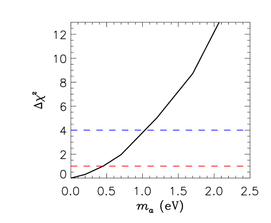
Figure 8: One-dimensional likelihood analysis for the hadronic axion model obeying Eq. (1). Shown is $\Delta\chi^{2}=\chi^{2}-\chi_{0}^{2}$ as a function of $m_{a}$ where $\chi_{0}^{2}$ refers to the best-fit model. In this 1D analysis the 95% excluded region is at $\Delta\chi^{2}>4$, and the 68% excluded region at $\Delta\chi^{2}>1$, as indicated by the horizontal dashed lines.

5 Summary

We have studied structure-formation limits on axions or other scalar particles that have a small mass and that couple to pions by virtue of the Lagrangian Eq. (4). Our main result is the exclusion range in the two-dimensional $f_{a}$-$m_{a}$ parameter space shown in Fig. 7 where the axion-pion coupling strength of Eq. (5) was assumed, i.e. this is an exclusion range in the parameter space of axion mass and axion-pion coupling. Assuming in addition the standard $m_{a}$-$f_{a}$ relationship of Eq. (1), we find a limit on the axion mass of $m_{a}<1.05$ eV (95% CL), corresponding to $f_{a}>5.7\times 10^{6}$ GeV.

A comparable axion mass limit is obtained from the requirement that excessive energy losses of horizontal branch stars in globular clusters should be avoided [12]. However, the globular-cluster limit depends on the axion-photon interaction that is rather model dependent.

The neutrino observations of supernova 1987A provide restrictive limits on the axion-nucleon interaction, suggesting $m_{a}\,\hbox to0.0pt{\lower 3.7pt\hbox{$\mathchar 0\relax\sim$}\hss}\raise 1.0pt\hbox{$<$}\,0.01$ eV or $f_{a}\,\hbox to0.0pt{\lower 3.7pt\hbox{$\mathchar 0\relax\sim$}\hss}\raise 1.0pt\hbox{$>$}\,0.6\times 10^{9}$ GeV if one assumes generic coupling strengths between axions and nucleons. However, the supernova argument may leave open the “hadronic axion window” of about $3\times 10^{5}~{}{\rm GeV}\,\hbox to0.0pt{\lower 3.7pt\hbox{$\mathchar 0\relax\sim$}\hss}\raise 1.0pt\hbox{$<$}\,f_{a}\,\hbox to0.0pt{\lower 3.7pt\hbox{$\mathchar 0\relax\sim$}\hss}\raise 1.0pt\hbox{$<$}\,3\times 10^{6}~{}{\rm GeV}$ [17, 18]. Our result closes this window, at least for generic values of the axion-nucleon and axion-pion couplings.

More importantly, we have provided a new limit on axion parameters based on a different interaction channel than previous limits and based on different data and assumptions. Every experimental measurement and every astrophysical or cosmological argument has its own systematic uncertainties and its own recognized or un-recognized loop holes. Therefore, to corner axions it is certainly important to use as many independent interaction channels and as many different approaches as possible.

An ongoing experimental axion search, the CERN Axion Solar Telescope (CAST), is based on the axion-photon interaction. It has reported first limits for $m_{a}\,\hbox to0.0pt{\lower 3.7pt\hbox{$\mathchar 0\relax\sim$}\hss}\raise 1.0pt\hbox{$<$}\,0.02$ eV [47]. In the second phase it will cover axion masses up to approximately 1 eV. It is noteworthy that our new limit is almost identical with the upper mass range that can be reached with CAST, i.e. the CAST search and our new limit are nicely complementary.

References

References

- [1] S. Hannestad, “Neutrinos in cosmology,” New J. Phys. 6, 108 (2004) [hep-ph/0404239].
- [2] S. Hannestad and G. Raffelt, “Cosmological mass limits on neutrinos, axions, and other light particles,” JCAP 0404 (2004) 008 [hep-ph/0312154].
- [3] R. D. Peccei and H. R. Quinn, “CP Conservation in the presence of pseudoparticles,” Phys. Rev. Lett. 38 (1977) 1440.
- [4] R. D. Peccei and H. R. Quinn, ‘Constraints imposed by CP conservation in the presence of pseudoparticles,” Phys. Rev. D 16 (1977) 1791.
- [5] S. Weinberg, “A new light boson?,” Phys. Rev. Lett. 40 (1978) 223.
- [6] F. Wilczek, “Problem of strong P and T invariance in the presence of instantons,” Phys. Rev. Lett. 40 (1978) 279.
- [7] M. Kamionkowski and J. March-Russell, “Planck scale physics and the Peccei-Quinn mechanism,” Phys. Lett. B 282 (1992) 137 [hep-th/9202003].
- [8] S. M. Barr and D. Seckel, “Planck scale corrections to axion models,” Phys. Rev. D 46 (1992) 539.
- [9] J. Gasser and H. Leutwyler, “Quark masses,” Phys. Rept. 87 (1982) 77.
- [10] H. Leutwyler, “The ratios of the light quark masses,” Phys. Lett. B 378 (1996) 313 [hep-ph/9602366].
- [11] S. Eidelman et al. [Particle Data Group], “Review of particle physics,” Phys. Lett. B 592 (2004) 1.
- [12] G. G. Raffelt, “Particle physics from stars,” Annu. Rev. Nucl. Part. Sci. 49 (1999) 163 [hep-ph/9903472].
- [13] J. E. Kim, “Weak interaction singlet and strong CP invariance,” Phys. Rev. Lett. 43 (1979) 103.
- [14] M. A. Shifman, A. I. Vainshtein and V. I. Zakharov, “Can confinement ensure natural CP invariance of strong interactions?,” Nucl. Phys. B 166 (1980) 493.
- [15] A. R. Zhitnitsky, “On possible suppression of the axion hadron interactions,” Sov. J. Nucl. Phys. 31 (1980) 260 [Yad. Fiz. 31 (1980) 497].
- [16] M. Dine, W. Fischler and M. Srednicki, “A simple solution to the strong CP problem with a harmless axion,” Phys. Lett. B 104 (1981) 199.
- [17] T. Moroi and H. Murayama, “Axionic hot dark matter in the hadronic axion window,” Phys. Lett. B 440 (1998) 69 [hep-ph/9804291].
- [18] S. Chang and K. Choi, “Hadronic axion window and the big bang nucleosynthesis,” Phys. Lett. B 316 (1993) 51 [hep-ph/9306216].
- [19] M. Carena and R. D. Peccei, “The effective Lagrangian for axion emission from SN 1987A,” Phys. Rev. D 40 (1989) 652.
- [20] M. S. Turner, “Thermal production of not so invisible axions in the early universe,” Phys. Rev. Lett. 59 (1987) 2489 [Erratum-ibid. 60 (1988) 1101].
- [21] E. Massó, F. Rota and G. Zsembinszki, “On axion thermalization in the early universe,” Phys. Rev. D 66 (2002) 023004 [hep-ph/0203221].
- [22] S. Hannestad and J. Madsen, “Neutrino decoupling in the early universe,” Phys. Rev. D 52 (1995) 1764 [astro-ph/9506015].
- [23] J. Preskill, M. B. Wise and F. Wilczek, “Cosmology of the invisible axion,” Phys. Lett. B 120 (1983) 127.
- [24] L. F. Abbott and P. Sikivie, “A cosmological bound on the invisible axion,” Phys. Lett. B 120 (1983) 133.
- [25] M. Dine and W. Fischler, “The not-so-harmless axion,” Phys. Lett. B 120 (1983) 137.
- [26] R. L. Davis, “Cosmic axions from cosmic strings,” Phys. Lett. B 180 (1986) 225.
- [27] R. Bradley et al., “Microwave cavity searches for dark-matter axions,” Rev. Mod. Phys. 75 (2003) 777.
- [28] E. W. Kolb and M. S. Turner, The Early Universe (Addison Wesley, 1990).
- [29] S. Hannestad, “Cosmological limit on the neutrino mass,” Phys. Rev. D 66 (2002) 125011 [astro-ph/0205223].
- [30] S. Hannestad, “Neutrino masses and the number of neutrino species from WMAP and 2dFGRS,” JCAP 0305 (2003) 004 [astro-ph/0303076].
- [31] S. Hannestad, “Cosmological bounds on masses of neutrinos and other thermal relics,” contributed to the Proc. of SEESAW25: International Conference on the Seesaw Mechanism and the Neutrino Mass, Paris, France, 10–11 June 2004 [hep-ph/0409108].
- [32] U. Seljak and M. Zaldarriaga, “A line of sight approach to cosmic microwave background anisotropies,” Astrophys. J. 469 (1996) 437 [astro-ph/9603033]. See also the CMBFAST website at http://cosmo.nyu.edu/matiasz/CMBFAST/cmbfast.html
- [33] S. Hannestad, “Stochastic optimization methods for extracting cosmological parameters from cosmic microwave background radiation power spectra,” Phys. Rev. D 61 (2000) 023002.
- [34] M. Tegmark et al. [SDSS Collaboration], “Cosmological parameters from SDSS and WMAP,” Phys. Rev. D 69 (2004) 103501 [astro-ph/0310723].
- [35] M. Tegmark et al. [SDSS Collaboration], “The 3D power spectrum of galaxies from the SDSS,” Astrophys. J. 606 (2004) 702 [astro-ph/0310725].
- [36] M. Colless et al., “The 2dF Galaxy Redshift Survey: Final data release,” astro-ph/0306581.
- [37] C. L. Bennett et al., “First year Wilkinson Microwave Anisotropy Probe (WMAP) observations: Preliminary maps and basic results,” Astrophys. J. Suppl. 148 (2003) 1 [astro-ph/0302207].
- [38] D. N. Spergel et al., “First year Wilkinson Microwave Anisotropy Probe (WMAP) observations: Determination of cosmological parameters,” Astrophys. J. Suppl. 148 (2003) 175 [astro-ph/0302209].
- [39] L. Verde et al., “First year Wilkinson Microwave Anisotropy Probe (WMAP) observations: Parameter estimation methodology,” Astrophys. J. Suppl. 148 (2003) 195 [astro-ph/0302218].
- [40] A. Kogut et al., “Wilkinson Microwave Anisotropy Probe (WMAP) first year observations: TE polarization,” Astrophys. J. Suppl. 148 (2003) 161 [astro-ph/0302213].
- [41] G. Hinshaw et al., “First year Wilkinson Microwave Anisotropy Probe (WMAP) observations: Angular power spectrum,” Astrophys. J. Suppl. 148 (2003) 135 [astro-ph/0302217].
- [42] A. G. Riess et al. [Supernova Search Team Collaboration], “Type Ia supernova discoveries at z¿1 from the Hubble Space Telescope: Evidence for past deceleration and constraints on dark energy evolution,” Astrophys. J. 607 (2004) 665 [astro-ph/0402512].
- [43] A. Goobar, E. Mörtsell, R. Amanullah, M. Goliath, L. Bergström and T. Dahlén, “SNOC: A Monte-Carlo simulation package for high-z supernova observations,” Astron. Astrophys. 392 (2002) 757 [astro-ph/0206409]. Code available at http://www.physto.se/ariel/snoc/
- [44] R. A. Croft et al., “Towards a precise measurement of matter clustering: Lyman-alpha forest data at redshifts 2–4,” Astrophys. J. 581, 20 (2002) [astro-ph/0012324].
- [45] N. Y. Gnedin and A. J. S. Hamilton, “Matter power spectrum from the Lyman-alpha forest: Myth or reality?,” Mon. Not. R. Astr. Soc. 334 (2002) 107 [astro-ph/0111194].
- [46] W. L. Freedman et al., “Final results from the Hubble Space Telescope key project to measure the Hubble constant,” Astrophys. J. 553 (2001) 47 [astro-ph/0012376].
- [47] K. Zioutas et al. [CAST Collaboration], “First results from the CERN axion solar telescope (CAST),” Phys. Rev. Lett., in press (2005) [hep-ex/0411033].