Bottom-Up Approach to Moduli Dynamics
in Heavy Gravitino Scenario :
Superpotential, Soft Terms and Sparticle Mass Spectrum

Abstract

The physics of moduli fields is examined in the scenario where the gravitino is relatively heavy with mass of order 10 TeV, which is favored in view of the severe gravitino problem. The form of the moduli superpotential is shown to be determined, if one imposes a phenomenological requirement that no physical CP phase arise in gaugino masses from conformal anomaly mediation. This bottom-up approach allows only two types of superpotential, each of which can have its origins in a fundamental underlying theory such as superstring. One superpotential is the sum of an exponential and a constant, which is identical to that obtained by Kachru et al. (KKLT), and the other is the racetrack superpotential with two exponentials. The general form of soft supersymmetry breaking masses is derived, and the pattern of the superparticle mass spectrum in the minimal supersymmetric standard model is discussed with the KKLT-type superpotential. It is shown that the moduli mediation and the anomaly mediation make comparable contributions to the soft masses. At the weak scale, the gaugino masses are rather degenerate compared to the minimal supergravity, which bring characteristic features on the superparticle masses. In particular, the lightest neutralino, which often constitutes the lightest superparticle and thus a dark matter candidate, is a considerable admixture of gauginos and higgsinos. We also find a small mass hierarchy among the moduli, gravitino, and superpartners of the standard-model fields. Cosmological implications of the scenario are briefly described.

I Introduction

Low-energy supersymmetry provides us with one of the most attractive candidates for the fundamental theory beyond the standard model [1]. However supersymmetry must be a broken symmetry below the electroweak scale due to the absence of any experimental signatures. Supersymmetry breaking is expressed by soft terms which do not reintroduce quadratic divergences [2] and spoil the Planck/weak scale hierarchy [3]. These soft breaking terms consist of gaugino masses, scalar masses, and scalar trilinear couplings. Generic forms of soft breaking terms lead to new contributions and sometimes disastrous phenomenological effects to flavor-changing rare processes [4] as well as to CP violation [5]. To satisfy the experimental constraints and to make supersymmetric models viable, supersymmetry-breaking terms are forced to have special properties, which could be realized in various ways proposed in the literature.

In the context of supergravity and superstring theory, there exists the gravitino, namely, the supersymmetric partner of the graviton. It interacts with all particle species through tiny Planck-suppressed couplings and may be hard to be observed in collider experiments (see, however, [6].)  On the other hand, the gravitino is too easily “detected” in a cosmological sense and, in turn, that leads to severe constraints on its property in almost all supersymmetric theories [7]. This gravitino problem exists even in the inflationary Universe. If the gravitino is stable, its relic abundance has to be small not to contribute too much to the energy density of the Universe [8]. This can be achieved either if the gravitino mass is sufficiently light [8], or if the reheating temperature of the inflation is low enough to suppress the regeneration of gravitinos in the thermal bath [9]. For an unstable gravitino, the most severe constraint comes from the big-bang nucleosynthesis. If gravitinos decay with electromagnetic and/or hadronic showers during or after the nucleosynthesis epoch, the decay products would spoil the successful predictions of the big-bang nucleosynthesis by destroying synthesized light elements [7, 10, 11, 12, 13]. This argument puts a severe constraint on the gravitino abundance, which may be suppressed by invoking the inflation with sufficiently low reheating temperature. The constraint becomes relaxed and eventually disappears as the gravitino mass increases and it decays earlier. A heavy gravitino with mass of order 10 TeV can therefore greatly ameliorate the problem.

Supersymmetric theories also include particles with masses around the electroweak scale and with suppressed couplings to ordinary matter. They are generally called moduli fields, the existence of which may be related to the degeneracy of vacua parameterized by symmetries in high-energy theory. Therefore the moduli potential is flat in perturbation theory and only lifted by non-perturbative effects or supersymmetry breaking, which induces masses of moduli fields around the supersymmetry-breaking scale. It is known that the existence of moduli leads to serious cosmological difficulties [14] with their suppressed couplings and resultant long lifetime. Moduli fields start to oscillate when the expansion rate of the Universe becomes smaller than moduli masses. The coherent oscillations decay into ordinary particles after the nucleosynthesis occurred for moduli masses around the electroweak scale. With a natural value of the initial amplitude of moduli, induced huge entropy destroys the great success of the big-bang nucleosynthesis as a heavy gravitino does. This is the cosmological moduli problem. A simple and attractive way to evade the problem is to make all moduli sufficiently heavy so that the moduli decay before the nucleosynthesis [15, 16, 17, 18, 19]. The masses of moduli fields might naively be expected to be of the same order of other supersymmetry-breaking mass parameters, especially a similar order to the gravitino mass as in the hidden sector models. However there could be some hierarchy between them, crucially depending on the form of moduli potential which originates from supersymmetry-breaking dynamics. In these ways, cosmological arguments may be strong enough to discriminate dynamics of supersymmetry breaking.

In this paper, we consider the physics of moduli fields in the heavy gravitino scenario, i.e. with supersymmetry-breaking scale higher than the electroweak scale. This may be rather a common situation in supersymmetric theories, including supergravity and superstring theory. The only few exceptions include, e.g. supersymmetry breaking with strongly-coupled gauge dynamics in a low-energy regime [20]. The heavy gravitino generally implies that moduli fields also have their masses around the gravitino mass scale, and therefore the cosmological gravitino/moduli problems may be solved by making these fields sufficiently heavy. As mentioned above, the masses of moduli fields crucially depend on their potential form, which is supposed to arise from (non-perturbative) dynamics of supersymmetry breaking. There have been various proposals for potential forms derived from specific non-trivial dynamics in high-energy theory. A well-known example is for the dilaton modulus field in string-inspired theories, which modulus is stabilized by (multiple) gaugino condensations [21, 22, 23], non-perturbative corrections to Kähler terms [24], and so on. Recent development of the flux compactifications in type IIB superstring theory reveals another possibility, in which the dilaton is fixed in the presence of fluxes, and the moduli stabilization can be achieved by some additional non-perturbative effects [25, 26]. Patterns of supersymmetry breaking by minimizing scalar potential have been discussed in Ref. [27].

We pursue, in a way, an opposite approach in that the possible form of moduli potential is highly constrained from a phenomenological viewpoint without referring to any specific dynamics at high-energy regime. For that purpose, it is a key ingredient to take into account the supersymmetry-breaking effects associated with the superconformal anomaly [28]. The soft mass parameters from the anomaly mediation are loop suppressed (because of being related to quantum anomalies) relative to the gravitino mass. It should be noted that this anomaly-mediated contribution ubiquitously exists in all scenarios of supersymmetry breaking. Such unavoidable anomaly effects cannot be neglected in the heavy gravitino models and may provide significant corrections to observable quantities measured at high accuracy [29]. Among them, the violation of CP invariance is one of the most notable quantities, including the electric dipole moments of nucleons, atoms, and charged leptons. The experimental results indicate that complex phases of soft mass parameters are tightly constrained so that supersymmetric contributions to CP-violating observables do not exceed the predictions of the standard model. On the basis of such phenomenological results, we will find in Section II that the superpotential of moduli fields which participate in supersymmetry breaking is uniquely determined (up to a Kähler transformation) by requiring CP be automatically conserved.

It is worth mentioning that the possible form of a moduli potential is completely fixed irrespectively of the stabilization and specific dynamics of moduli fields. Interestingly enough, we will see in Section III that the obtained potential, however, does stabilize the moduli and also cause supersymmetry breaking. Furthermore the superpotential has its origin in ordinary field theory and superstring theory. In particular, it has recently been shown [25, 26] that some classes of superstring compactification in the presence of non-trivial fluxes generate the above-mentioned superpotential for Kähler moduli fields. It may be a surprising result that two completely different perspectives, a top-down one from string theory and a bottom-up one from experimental observations, derive the same and unique form of moduli potential.

It is found in Section IV that the mass spectrum in the model with the uniquely-determined superpotential exhibits two interesting types of small hierarchies among superparticles, gravitino, and moduli fields. The lightest particles are gauginos and scalar partners of quarks and leptons with masses around the electroweak or TeV scale. These mass scales are suppressed roughly by one-loop factors compared to the gravitino mass due to the loop-suppressed contribution of the anomaly mediation. This first hierarchy is favorable for solving the gravitino problem as stated above. The heaviest states are moduli whose masses are O(10) times that of the gravitino. This second hierarchical factor is roughly determined by the logarithm of the ratio between the Planck and electroweak scales. That is naturally obtained by minimizing the uniquely determined moduli potential. Since the moduli become heavy in the vacuum, they have suppressed contributions to supersymmetry breaking. We find that the anomaly and moduli mediations induce numerically similar sizes of soft mass parameters for visible-sector superpartners, which are of the order of the electroweak scale. It is noted that, as mentioned above, our analysis covers a mass spectrum derived from some superstring theory in flux compactifications. The problem of the tachyonic slepton, which is a serious problem in the model of pure anomaly mediation, is ameliorated. More interestingly, our scenario predicts the lightest neutralino with a significant composition of higgsinos as the lightest supersymmetric particle in a wide range of parameter space. Together with this issue, we study in Section V new cosmological implications of our model with heavy moduli fields.

II The Model

A Four-dimensional supergravity

The dynamics of gravitino and moduli fields is described by $N=1$ four-dimensional supergravity. The gauge-invariant Lagrangian, in particular the scalar potential, is most simply written down with the compensator formalism of supergravity [30]. Larger gauge symmetries make the theory easily analyzed, and the usual Poincaré supergravity is obtained by fixing redundant conformal/Poincaré local gauge symmetries. Let us consider a single chiral superfield $X$, for simplicity, but it is straightforward to include multiple superfields in the Lagrangian. The most general supergravity Lagrangian is given by

$$e^{-1}{\cal L}_{c}\,=\,\int\!d^{4}\theta\,\Phi^{\dagger}\Phi\,f(X,X^{\dagger})\,+\int\!d^{2}\theta\,\Phi^{3}\,W(X)+{\rm h.c.},$$ (1)

where $e$ is the determinant of the vierbein field and the reduced Planck mass is set to unity. We use as usual the same notation $X$ for a chiral superfield, scalar component, and its vacuum expectation value. $W(X)$ is the superpotential of $X$, and $f$ the supergravity $f$ function which is related to the Kähler potential $K$ in the Einstein frame

$$f(X,X^{\dagger})\,=\,-3e^{-K(X,X^{\dagger})/3}.$$ (2)

The symbols $\int\!d^{4}\theta$ and $\int\!d^{2}\theta$ mean the uses of $D$- and $F$-type action formulas of superconformal tensor calculus. The chiral superfield $\Phi$ is the conformal compensator multiplet and its value is fixed by the part of superconformal gauge transformation such as dilatation so that $\Phi=1+F_{\phi}\theta^{2}$. In the discussion below, we assume the flat gravitational background and will drop $e$ from the action. The Lagrangian (1) contains the following terms of auxiliary $F$ components

$${\cal L}_{c}\,=\,fF_{\phi}^{*}F_{\phi}+f_{X}F_{\phi}^{*}F_{X}+f_{\bar{X}}F_{\phi}F_{X}^{\dagger}+f_{X\bar{X}}F_{X}^{\dagger}F_{X}+(3WF_{\phi}+W_{X}F_{X}+{\rm h.c.})+\cdots.$$ (3)

The lower indices of $f$ and $W$ denote the field derivatives. The equations of motion are thus given by

$$F_{X} \,=\, -e^{K/3}K_{X\bar{X}}^{\,-1}(W_{X}+WK_{X})^{\dagger},$$ (4)

$$F_{\phi}\, \,=\, e^{K/3}W^{*}+\frac{1}{3}K_{X}F_{X}.$$ (5)

Substituting these equations back into (3), one obtains the scalar potential of the $N=1$ four-dimensional supergravity

$$V\,=\,e^{K/3}\Big{[}\,(W_{X}+WK_{X})^{\dagger}K_{X\bar{X}}^{\,-1}(W_{X}+WK_{X})-3|W|^{2}\,\Big{]}$$ (6)

in the conformal frame. The canonical potential in the Einstein frame is easily obtained by field-dependent Weyl rescaling. Assuming that the vacuum expectation value of the scalar potential vanishes, a location of the potential minimum is unchanged by this Weyl rescaling, and thus we will use the conformal frame in most of the subsequent discussions.

As seen from the above formulation, there are two types of supersymmetry-breaking $F$ terms. One is the chiral superfield $F$ component $F_{X}$, where $X$ participates in supersymmetry breaking with a non-vanishing $F_{X}$. Another is the compensator contribution $F_{\phi}$ that should be taken into account in any supersymmetry-breaking scenario. In particular, since $F_{\phi}$ gives a gravitino mass scale, its contribution to other superparticles is important in the heavy gravitino scenario. In the present work, that will play a key role to determine the potential form of moduli fields.

In the superconformal framework, the Lagrangian of vector multiplets, especially for gaugino masses, includes the gauge kinetic function $S$,

$${\cal L}_{v}\,=\,\int\!d^{2}\theta\,S\Big{(}X,\frac{\mu}{\Lambda\Phi}\Big{)}W^{\alpha}W_{\alpha}+{\rm h.c.}.$$ (7)

At the classical level, the compensator $\Phi$ does not appear in the gauge kinetic term as the gauge chiral superfield $W^{\alpha}$ has a chiral weight $\frac{3}{2}$. It turns out that the dependence of $\Phi$ comes out radiatively through the ultraviolet cutoff $\Lambda$ ($\mu$ is the renormalization scale). In this paper, we take for simplicity $S\propto X$ by holomorphic field redefinition. Note however that this choice does not necessarily means $X$ is a dilaton in the four-dimensional supergravity, whose vacuum expectation value determines the gauge coupling constant $g$. One may instead suppose, e.g. $S=\frac{1}{4g^{2}}+X$, but there are only quantitative difference between these two forms of gauge kinetic function. In particular, the following analysis of potential forms of moduli is completely unchanged.

A gaugino receives two types of supersymmetry-breaking mass from the Lagrangian (7). As mentioned above, the effect of the compensator multiplet appears only through the renormalization and induces gaugino masses which are determined by super Weyl anomaly. The total gaugino mass $M_{\lambda}$ in the canonically normalized basis is found

$$M_{\lambda}\,=\,\frac{F_{X}}{2X_{R}}+\frac{\beta_{g}}{g}F_{\phi},$$ (8)

where $\beta_{g}$ is the gauge beta function ($\beta_{g}=\frac{\partial g}{\partial\ln\mu}$). We have defined the real part of $X$ as $X_{R}\equiv{\rm Re}\,X$. Gaugino masses given above are evaluated at a high-energy scale. Here we simply neglect threshold corrections from high-energy theory. When only the moduli- and anomaly-mediated contributions are taken into account, higher-order corrections and threshold effects do not disturb the discussion about complex phases of $M_{\lambda}$. These corrections just modify the mass spectrum slightly.

B Gaugino mass phases and moduli potential

We would like to investigate the dynamics of moduli fields. As can be seen in (1), that is determined by two functions of the moduli field $X$; Kähler potential $K(X,X^{\dagger})$ and superpotential $W(X)$. We first note that the assumption that $X$ is a modulus gives a constraint on its Kähler potential. The existence of moduli fields may be related to the degeneracy of vacua which are parameterized by symmetries of theory. Then imaginary parts of moduli fields often transform non-linearly under these flavor symmetries which dictate the moduli Kähler potential in low-energy effective theory as

$$K(X,X^{\dagger})\,=\,K(X+X^{\dagger})$$ (9)

with a real function $K$. We assume that this shift symmetry would be broken only to an extent that it does not induce any observable effects. On the other hand, the moduli superpotential $W(X)$ is not allowed by the shift symmetry as it should be, and may be generated due to symmetry-breaking effects in effective theory. Thus, moduli superpotential does not generally have any restrictions and its promising forms have been discussed in model-dependent ways so as to stabilize moduli expectation values, to have moduli supersymmetry breaking, etc. We will show below that, in the heavy gravitino scenario, a possible form of moduli superpotential can be determined model-independently and also without taking any particular assumption of the moduli Kähler potential (9).

To this end, it is important to notice that there are two types of supersymmetry-breaking masses of gauginos (8). In the heavy gravitino scenario, these two contributions may be comparable in size to each other. Therefore their relative phase value gives rise to sizable complex phases of gaugino masses. If there is only one gaugino in the theory, its mass can be made real with $U(1)_{R}$ rotation. However, realistic models such as supersymmetric standard models may contain multiple gauge factors. In this case, phases of gaugino masses are generally not aligned because the anomaly mediated contributions ($F_{\phi}$ terms) are proportional to gauge beta functions which are diverse from each other. Consequently, all but one gaugino mass phase cannot be rotated away from the Lagrangian and remain physical observables. It is easily found that the situation is not improved even if the standard gauge groups are embedded into a unified gauge group in a high-energy regime. This is because anomaly mediated contributions are determined only by low-energy quantities and decouple from high-energy physics. In other words, threshold effects at the unification scale split the complex phases of low-energy gaugino masses. It might be an interesting possibility that non-vanishing phases of gaugino masses are detectable in future particle experiments [29]. But, in that case, other parameters should be carefully chosen so as to satisfy various severe constraints which come from approximate CP conservations observed in nature.

In this work, we pursue a more natural way that each gaugino mass has no more tiny phase; namely, all gaugino mass phases are aligned, which are rotated away by a single $R$ rotation. It is clear from (8) that this is achieved by realizing a tiny relative phase between the two supersymmetry-breaking $F$ terms. The ratio is simply written as

$$\frac{F_{\phi}}{F_{X}}\,=\,-[\ln(fG_{\bar{X}})]_{X},$$ (10)

where $G$ is the supergravity Kähler potential: $G\equiv K+\ln|W|^{2}$. But it is suitable for practical purpose that the ratio is rewritten with $K$ and $W$;

$$\frac{F_{\phi}}{F_{X}}\,=\,\frac{K_{X}}{3}-\frac{K_{X\bar{X}}}{K_{\bar{X}}+\big{(}\frac{W_{X}}{W}\big{)}^{\dagger}}.$$ (11)

Since we now consider $X$ as a moduli field, any derivatives of the Kähler potential $K$ are real valued, irrespectively of its detailed form. When this ratio of two $F$ terms is real, all gauginos receive supersymmetry-breaking masses with aligned complex phases and they can be made real. We find from Eq. (11) that this is the case if

$$\frac{W_{X}}{W}\,=\,{\rm real}.$$ (12)

The condition (12) must be satisfied in the vacuum of the supergravity scalar potential. With the moduli Kähler potential (9), it is easy to first minimize the scalar potential with respect to the imaginary part of $X$ ($X_{I}\equiv{\rm Im}\,X$);

$$0\,=\,\frac{\partial\,V}{\partial X_{I}}\,=\,-ie^{K/3}K_{X\bar{X}}^{\,-1}\Big{[}\,(WK_{X}+W_{X})(W_{X}K_{X}+W_{XX})^{\dagger}+3K_{X\bar{X}}W_{X}W^{*}-{\rm h.c.}\,\Big{]}.$$ (13)

This leads to a condition

$$\bigg{(}K_{X}K_{\bar{X}}-3K_{X\bar{X}}+K_{\bar{X}}\frac{W_{XX}}{W_{X}}\bigg{)}|W|^{2}\frac{W_{X}}{W}+|W_{X}|^{2}\frac{W_{XX}}{W_{X}}\;=\;{\rm real}.$$ (14)

It is found that when gaugino mass phases are small, namely, the condition (12) is satisfied, the following equation:

$$\frac{W_{XX}}{W_{X}}\;=\;{\rm real}$$ (15)

is also satisfied in the vacuum as long as the moduli field causes supersymmetry breaking ($F_{X}\neq 0$). The reverse is also true that if one has superpotential satisfying $W_{XX}/W_{X}$ = real, then $W_{X}/W$ takes a real value and the condition for aligned gaugino masses is certainly realized at the extrema of supergravity potential. It is important that the equation (15) is integrable. That is, since the superpotential $W(X)$ is a holomorphic function, $W_{XX}/W_{X}$ should be a real constant with respect to $X$. (It may be rather unlikely that the reality condition is satisfied with real coupling constants and/or vacuum expectation values. That might be realized only in a special circumstance where an original theory contains real parameters and would also require additional requirements.)  We thus find the most general moduli superpotential leading to aligned gaugino masses

$$W(X)\,=\,ae^{-bX}+c,$$ (16)

where $a$, $b$, and $c$ are $X$-independent factors and, in particular, $b$ must be real. The negative sign in front of $b$ is just a convention. We have found that, with the moduli superpotential (16), all gaugino masses can be made real in the extrema of supergravity scalar potential and do not induce large CP-violating operators. It should be noted that the result has been derived without specifying a detailed form of the moduli Kähler potential. In the complete analysis of scalar potential with a fixed form of $K$, one should check whether it is a (at least local) minimum of the potential. That will be examined in the next section.

We have so far focused only on the phases of gaugino mass parameters. Similar arguments are also applied to other supersymmetry-breaking parameters. Let us define, as usual, a holomorphic soft breaking parameter as a ratio of a coupling of holomorphic supersymmetry-breaking term to a corresponding superpotential one. These soft-breaking parameters are unaffected by phase redefinitions of chiral superfields. We will explicitly show in the next section that, if the condition (12) for aligned gaugino masses is satisfied, all complex phases of holomorphic soft parameters are aligned to that of gaugino masses and become real once gaugino masses are rotated to be real by $R$ rotation.

Our argument above is based on the supergravity scalar potential which is controlled by two functions $K(X,X^{\dagger})$ and $W(X)$. It is known that the supergravity potential is invariant under Kähler transformation involving these two functions: $K\to K+\Gamma(X)+\bar{\Gamma}(\bar{X})$ and $W\to e^{-\Gamma(X)}W$ with an arbitrary function $\Gamma(X)$. Noting that the Kähler potential depends on the moduli in the form of (9), the only possible transformation is given by $\Gamma(X)=b^{\prime}X$ with a real factor $b^{\prime}$. After such transformation, we have the superpotential

$$W(X)\,=\,a_{1}e^{-b_{1}X}+a_{2}e^{-b_{2}X},$$ (17)

where $a_{1,2}$ and $b_{1,2}$ are complex and real $X$-independent factors, respectively. This is another form of moduli superpotential which satisfies our requirement that CP invariance is not broken by the moduli physics. That is, complex phases of soft supersymmetry-breaking parameters are aligned in the vacuum of supergravity potential. One should note that this form of the moduli superpotential as a solution to the supersymmetric CP problem was recognized in Ref. [32]

C Origins of moduli superpotential

In the previous section we found two types of superpotential for moduli fields. With these forms of superpotential, one obtains phenomenologically favorable results; namely, CP-violating effects of moduli are automatically suppressed in the vacuum. On the other hand, more formal aspects, e.g. the questions of whether such potentials are derived from some high-energy theory and which of these two forms is relevant, may depend on the property of moduli fields and its natural form of Kähler potentials.

For some specific moduli fields, the superpotential forms (16) and (17) have been discussed in the literature. Among these is that $X$ is the dilaton superfield in four-dimensional effective theory of superstring. In this case, an exponential factor $e^{-bX}$ emerges through gaugino condensation [21, 22, 23] where the constant $b$ is inversely proportional to the gauge beta function and therefore a real parameter, just as needed. A likely example of dilaton stabilization along this line is the racetrack mechanism [22] with superpotential of the form (17). However it was found that a realistic value of gauge coupling is achieved only in rather complicated models, for example, with more than two condensations. The constant $c$ term in (16) is also known to play important roles of the dilaton stabilization and supersymmetry breaking [23, 33]. We should note that such a type of superpotential with the constant term is obtained in a five-dimensional model [34] where $X$ is the radius modulus which determines the size of the compact fifth dimension.

As we mentioned in the introduction, it is revealed in perturbative string theory that there exist some massless moduli fields whose presence may be in contradiction to low-energy experiments. Recently, it has been discussed that all such moduli can be stabilized in some string compactifications with non-trivial fluxes. As an example, let us consider a class of type IIB orientifold compactification. The absence of non-trivial fluxes classically leads to supersymmetric vacua which are described by the dilaton modulus, complex structure (shape) moduli, and complexified Kähler (size) moduli. If three-form field strengths are turned on, they give rise to a tree-level superpotential $W_{0}$ [35]. Having this superpotential in hand, the vacuum is explored with effective four-dimensional supergravity potential. It is found that for a generic choice of fluxes, the minimization of potential fixes all shape moduli and the dilaton [25]. This scheme of stabilization sets the expectation value of the dilaton to a weak coupling and is under reliable control.

The above superpotential $W_{0}$ is, however, independent of the Kähler size moduli and they can take arbitrary values. One needs some additional potential which might be generated by stringy and quantum corrections to Kähler and/or superpotentials. It is suggested by Kachru-Kallosh-Linde-Trivedi (KKLT) in [26] that the Kähler size moduli can be stabilized by including non-perturbative corrections [36] to the tree-level superpotential. These corrections are known to depend on the size moduli and be controlled at weak coupling. Ref. [26] discussed two types of such non-perturbative effects: (i) D-brane instantons and (ii) gaugino condensation. In the case (i), the source of superpotential is D3-brane instantons wrapped on surfaces in the Calabi-Yau three-fold. The instanton-induced superpotential takes the form $W_{\rm np}=\sum a_{n}e^{-2\pi n\cdot\chi}$ where $\chi$ are the complexified volumes, which are natural holomorphic coordinates appearing in type IIB orientifold compactification. In the large volume limit, the shape moduli are stabilized by the leading contribution $W_{0}$. Accordingly one can use $W=W_{0}+W_{\rm np}$ as effective superpotential for the Kähler size moduli. In the case of (ii), the superpotential is supposed to be generated by non-perturbative effects in world-volume gauge theory on D7 branes. The gauge coupling in this theory depends on the volume $V$ and thus non-perturbative effects lead to a superpotential $W_{\rm np}\sim e^{-V/\beta}$. The constant $\beta$ is real and related to the gauge beta function which is of order $N_{c}$ for $SU(N_{c})$ gauge theory. For a small value of the flux superpotential $W_{0}$, the supersymmetric condition for a size modulus is satisfied with a large value of $V$.

In both cases, the non-perturbative contribution to superpotential is of the form $W_{\rm np}=ae^{-bX}$ (for the case (i), the leading order in the large volume limit). The effective superpotential is therefore given by $W=W_{0}+W_{\rm np}$. It is found that all the complex structure moduli and the ten-dimensional dilaton are frozen by the fluxes (the first term), which are essentially decoupled from low-energy effective theory and thus do not play any role in supersymmetry breaking, while the second term generated by non-perturbative stringy corrections can stabilize all remaining Kähler moduli which arise in low-energy effective theory. As we mentioned, $W_{0}$ is a constant with respect to the Kähler size moduli. Moreover the parameter $b$ in $W_{\rm np}$ is real in either case. Remarkably, the resulting moduli superpotential is exactly the same form as we have derived in the previous subsection by looking for phenomenologically preferable moduli potential.

In heterotic/M theory, there might also exist similar mechanism to stabilize all heterotic moduli to the proposal of KKLT. First, flux-induced superpotentials fix all shape moduli and in some cases also the size modulus, which is not the case for type IIB string. After including non-perturbative effects such as gaugino condensation and world-sheet instanton effects, all remaining moduli are shown to be stabilized [37]. See also other approaches, for example, using non-Kähler background with gaugino condensation to stabilize the dilaton modulus [38]. Anyway the resulting superpotential generally takes the common form, $W=W_{0}+W_{\rm np}$, and is consistent to our result (16) of CP-conserving moduli potential (now for the dilaton or radius modulus).

We finally comment on typical scales of dimensionful parameters as well as possible field-theoretical origins of the moduli superpotential. The exponential dependence of the moduli field is realized in various ways. As explained above, for the dilaton and related variables, that is induced by gaugino condensations or non-perturbative effects in supersymmetric gauge theories. Therefore a natural scale of the coefficient $a$ in (16) might be on the fundamental scale of the theory. On the other hand, the constant term $c$ is related to supersymmetry breaking and should be suppressed relative to the fundamental scale in order to have low-energy supersymmetry. The detailed analysis in the following sections will show that a small $c$ is, in fact, relevant to various phenomenology of the model. In the flux compactification, following the spirit of Refs. [39], a small constant $c$ may be obtained by cancellation among contributions from many fluxes. The suppression can also be achieved by similar dynamics which generate the exponential term, that is, an exponentially small $c$ is obtained by gaugino condensation in additional gauge factor. Another simple way to have a suppressed constant term comes from symmetry argument and is described by a Wess-Zumino model without introducing any extra gauge factors. Let us consider the following superpotential:

$$W_{c}\,=\,\lambda\psi(\bar{\phi}\phi-M^{2})+m\bar{\phi}\phi.$$ (18)

The last term in the right-hand side causes soft breaking of $R$ symmetry, and one expects a constant superpotential to be generated. Integrating out the massive fields, we actually obtain a constant superpotential $W_{c}=mM^{2}$. A suppressed value of $c$ is natural in a sense that the first and second terms in (18) are $R$ exact and the third softly breaks the $R$ invariance. It is noted that the superpotential (18) is the most general and renormalizable one, provided that one imposes the parity [$P(\psi)=+$, $P(\phi,\bar{\phi})=-$] in addition to the $R$ invariance [$R(\psi)=2$, $R(\phi,\bar{\phi})=0$].

III Moduli stabilization

A KKLT-type superpotential

1 Potential analysis

In the previous section, we have found that a moduli superfield $X$ is expected to have the following potentials for realistic phenomenology:

$$K\,=\,K(X+X^{\dagger}),\quad\quad W(X)\,=\,ae^{-bX}+c.$$ (19)

The superpotential form has been determined by the requirement of suppressing gaugino mass phases. In this section III, we will fully analyze the supergravity potential of moduli and investigate its phenomenological implications in the vacuum. The supergravity potential in the conformal frame now to be investigated is given by

$$V\,=\,e^{K/3}K_{X\bar{X}}^{\,-1}\left[\,|a|^{2}\big{(}b^{2}-bK_{X}-\kappa\big{)}e^{-b(X+X^{\dagger})}+|c|^{2}(bK_{X}-\kappa)-\kappa\big{(}ac^{*}e^{-bX}\!+{\rm h.c.}\big{)}\,\right],$$ (20)

where we have defined the real function $\kappa\equiv 3K_{X\bar{X}}-K_{X}K_{\bar{X}}+bK_{X}$. Note that only the last term depends on the imaginary part $X_{I}$ of the moduli field. Minimizing the potential with respect to $X_{I}$, we have

$$0\,=\,\frac{\partial\,V}{\partial X_{I}}\,=\,b\kappa e^{K/3}K_{X\bar{X}}^{\,-1}\big{(}iac^{*}e^{-bX}+{\rm h.c.}\big{)},$$ (21)

which determines the expectation value of $X_{I}$ as

$$a^{*}ce^{ibX_{I}}\,=\,\epsilon|ac|\qquad(\epsilon=\pm 1).$$ (22)

The sign of $\epsilon$ is chosen so that the extremum is a minimum, that is, the second derivative with respect to $X_{I}$ should be positive at the extremum. This results in the condition $\epsilon\kappa>0$. In the minimum of $X_{I}$, the moduli potential becomes

$$V(X_{R})\,=\,e^{K/3}K_{X\bar{X}}^{\,-1}\Big{[}\,|a|^{2}\big{(}b^{2}-bK_{X}-\kappa\big{)}e^{-2bX_{R}}+|c|^{2}(bK_{X}-\kappa)-2|ac|\epsilon\kappa e^{-bX_{R}}\Big{]}.$$ (23)

The analysis of $V(X_{R})$ is performed with specifying the moduli Kähler potential. In this paper, we take a simple assumption

$$f\,=\,-3(X+X^{\dagger})^{n/3},$$ (24)

often discussed in the literature. For example, in string effective theory framework, $n$ is an integer ($n=1,2,3$). Having this Kähler potential at hand, we find the minimum for a suppressed value of $c$, which is related to the gravitino mass scale. It is important that the minimization leads to a large value of $bX_{R}$ ($>0$), and also a negative $\epsilon$ from the minimum condition ($\epsilon\kappa>0$). We thus obtain the stabilized value of moduli which satisfies the following equation at the minimum

$$e^{-bX_{R}}\,=\,\frac{n}{2}\left|\frac{c}{a}\right|\frac{1}{bX_{R}}\bigg{[}1-\frac{n+2}{2}\frac{1}{bX_{R}}+{\cal O}\big{(}(bX_{R})^{-2}\big{)}\bigg{]}.$$ (25)

One can easily see that the second derivative with respect to $X_{R}$ is certainly positive at this extremum. The detailed analysis of the global structure of moduli potential will be performed in a later section where the hidden-sector contribution and thermal effects in the early Universe are included into the potential.

2 F terms and the vacuum energy

In the obtained vacuum, supersymmetry is broken due to the presence of the constant factor $c$. The non-vanishing $F$ terms are evaluated from the general formulas (4) and (5):

$$F_{X} \,=\, \frac{2c^{*}}{b(2X_{R})^{n/3}}\left(1-\frac{2n-1}{2}\frac{1}{bX_{R}}+\cdots\right),$$ (26)

$$F_{\phi}\, \,=\, \frac{c^{*}}{(2X_{R})^{n/3}}\left(1-\frac{5n}{6}\frac{1}{bX_{R}}+\cdots\right).$$ (27)

The supersymmetry-breaking scale is controlled by $c$. In the limit $c\to 0$, the vacuum goes to infinity and supersymmetry is restored. Thus the constant term $c$, which is allowed in a generic solution (16), is found to play important roles for the moduli stabilization and also moduli supersymmetry breaking. In the following discussion of moduli phenomenology, a key ingredient is the ratio of two $F$-term contributions, which is now given by

$$\frac{(F_{X}/X_{R})}{F_{\phi}}\,=\,\frac{2}{bX_{R}}\left(1-\frac{n-3}{6}\frac{1}{bX_{R}}+\cdots\right),$$ (28)

where the ellipsis denotes real factors of ${\cal O}((bX_{R})^{-2})$. We find in the vacuum that the moduli contribution to supersymmetry breaking is suppressed, by a large value of $bX_{R}$, relative to the gravity contribution of $F_{\phi}$. The anomaly mediated contribution to visible fields is also suppressed, by one-loop factors, relative to $F_{\phi}$. It is interesting that the supersymmetry breaking effects mediated by the moduli and conformal anomaly are comparable in size in the heavy gravitino scenario. The theory predicts neither pure anomaly mediation nor pure moduli dominance and has characteristic mass spectrum, as we will study in the next section.

The above potential analysis has not been concerned about the vacuum energy (the cosmological constant). At the minimum given above, the $F$ term of the $X$ field is suppressed, and thus the vacuum energy is negative. We therefore need to uplift the potential to make its vacuum expectation value zero. In the KKLT model [26], an anti-D3 brane is introduced to break supersymmetry explicitly to generate a positive contribution to the vacuum energy. Here we introduce hidden-sector fields with nonzero vacuum expectation values of $F$ terms. One can incorporate in the supergravity $f$ function the direct couplings between hidden-sector variables and the moduli field, without conflicting with viable phenomenology in the visible sector. The perturbative expansion about a hidden-sector field $Z$ gives a Kähler potential

$$f\;=\;-3(X+X^{\dagger})^{n/3}+H(X+X^{\dagger})|Z|^{2}+{\cal O}(|Z|^{4}),$$ (29)

with a real function $H$, while preserving the moduli dependence of Kähler terms in the form $X+X^{\dagger}$. The first term is the moduli Kähler potential at the leading order (24). To avoid introducing an additional CP phase, we assume that the vacuum expectation value of $Z$ is negligibly small compared to the Planck scale. Minimizing the supergravity potential with respect to the moduli $X$, we find that the vacuum is shifted by turning on $F_{Z}$, in which vacuum the $F$ terms are given by

$$F_{X} \,\simeq\, \frac{2c^{*}}{b(2X_{R})^{n/3}}+\frac{2H_{X}X_{R}}{nbc}|F_{Z}|^{2},$$ (30)

$$F_{\phi}\, \,\simeq\, \frac{c^{*}}{(2X_{R})^{n/3}}.$$ (31)

The requirement of vanishing cosmological constant can be fulfilled with a non-vanishing $F$ term of hidden-sector field; $|F_{Z}|^{2}\simeq 3|c|^{2}/(2X_{R})^{n/3}H$ at the minimum. Substituting it for $F_{X}$, we obtain the $F$ terms in the shifted vacuum, in particular, whose ratio becomes in the leading order

$$\frac{(F_{X}/X_{R})}{F_{\phi}}\,\simeq\,\frac{2}{bX_{R}}\bigg{(}1+\frac{3X_{R}H_{X}}{nH}\bigg{)}.$$ (32)

For example, $H\propto(X+X^{\dagger})^{l}$ gives a correction $\frac{(F_{X}/X_{R})}{F_{\phi}}=\frac{2}{bX_{R}}\big{(}1+\frac{3l}{2n}\big{)}$. Thus the moduli mediated contribution is still smaller than $F_{\phi}$ by large $bX_{R}$ suppression. Moreover the ratio of two $F$ terms remains real and does not disturb the phase alignment of supersymmetry-breaking soft mass parameters.

B Racetrack-type superpotential

Similar analysis can be performed for another solution of CP conservation, i.e., the racetrack type superpotential of moduli field (17):

$$W(X)\,=\,a_{1}e^{-b_{1}X}+a_{2}e^{-b_{2}X}.$$ (33)

We here take $|b_{1}|>|b_{2}|$ without loss of any generalities. If the moduli is stabilized with interplay between these two terms, low-energy supersymmetry requires large [${\cal O}(10)$] values both for $b_{1}X_{R}$ and $b_{2}X_{R}$ or only for $b_{1}X_{R}$. In the latter case, the coupling $a_{2}$ must be hierarchically suppressed. That is qualitatively very similar to the case of superpotential (16) in the previous subsection with $c$ being replaced by $a_{2}e^{-b_{2}X}\sim a_{2}$. A straightforward calculation, in fact, indicates that the stabilization and $F$-term equations are almost the same also quantitatively. Therefore it is sufficient to consider the case that both $b_{1}X_{R}$ and $b_{2}X_{R}$ become large. The minimization with respect to $X_{I}$ then leads to the condition $a_{1}^{*}a_{2}e^{i(b_{1}-b_{2})X_{I}}=-|a_{1}a_{2}|$. We assume the moduli Kähler potential (24) now for the superpotential (17). In this case, the moduli is stabilized at the minimum

$$e^{-(b_{1}-b_{2})X_{R}}\,=\,\left|\frac{a_{2}}{a_{1}}\right|\left[\frac{b_{2}}{b_{1}}+\frac{n(b_{1}-b_{2})}{2b_{1}}\frac{1}{b_{1}X_{R}}+{\cal O}\big{(}(b_{1}X_{R})^{-2}\big{)}\right],$$ (34)

and the $F$ terms read from the general formulas as

$$F_{X} \,=\, \frac{2na_{2}^{*}e^{-b_{2}X^{*}}}{b_{1}b_{2}(2X_{R})^{n/3+1}}\frac{b_{1}-b_{2}}{b_{1}}\left(1-\frac{n(b_{1}+2b_{2})}{2b_{2}}\frac{1}{b_{1}X_{R}}+\cdots\right),$$ (35)

$$F_{\phi}\, \,=\, \frac{a_{2}^{*}e^{-b_{2}X^{*}}}{(2X_{R})^{n/3}}\frac{b_{1}-b_{2}}{b_{1}}\left(1-\frac{n}{2}\frac{1}{b_{1}X_{R}}+\cdots\right).$$ (36)

It may be interesting to see that the ratio of $F$ terms becomes

$$\frac{(F_{X}/X_{R})}{F_{\phi}}\,=\,\frac{n}{b_{1}b_{2}X_{R}^{2}}\left(1-\frac{n(b_{1}+b_{2})}{2b_{1}b_{2}X_{R}}+\cdots\right).$$ (37)

Therefore the moduli become much heavier than the gravitino in contrast to the case with the superpotential (16), and the moduli mediated contribution to supersymmetry breaking is highly suppressed. This means that the superparticle mass spectrum is described dominantly in terms of the anomaly mediation. As is well known, that makes some scalar leptons tachyonic as long as low-energy theory is the minimal supersymmetric standard model without some additional sources of supersymmetry breaking. On these grounds, we will focus in this paper on the moduli superpotential of the form (16), with which potential the moduli physics gives rise to rich and significant effects on low-energy phenomenology.

IV Mass spectroscopy

A Gravitino and moduli masses

In the previous section, we considered the following Kähler and superpotential of moduli and hidden-sector fields:

$$f\;=\;-3(X+X^{\dagger})^{n/3}+(X+X^{\dagger})^{l}|Z|^{2},\qquad W(X)\,=\,ae^{-bX}+c,$$ (38)

where $n=1,2,3$. With these forms at hand, we simultaneously obtained the stabilized moduli, broken supersymmetry, and the vanishing cosmological constant in the vacuum of supergravity potential. There exist two types of supersymmetry-breaking contributions, $F_{X}/X_{R}$ and $F_{\phi}$, in this model. In particular, the superpotential puts these $F$ terms to be not independent at the vacuum and approximately satisfy the relation

$$\frac{F_{X}}{X_{R}}\,=\,\frac{2}{bX_{R}}\bigg{(}1+\frac{3l}{2n}\bigg{)}F_{\phi}.$$ (39)

It is important to notice that, in the vacuum, the leading terms in $F_{X}$ are canceled out in the large $bX_{R}$ limit, and the moduli contribution $F_{X}/X_{R}$ is suppressed by $bX_{R}$, compared to $F_{\phi}$. Then the moduli and hidden-sector $F$ terms are found to be small at the vacuum, and the gravitino mass is expressed as

$$m_{3/2}\,=\,|F_{\phi}|.$$ (40)

The moduli field is stabilized by non-perturbative effect plus the constant superpotential, latter of which is a trigger of supersymmetry breaking. Therefore a natural expectation might be that its mass is around the symmetry-breaking scale. We however obtain the moduli mass which reads from the Lagrangian (1)

$$m_{X_{R}}\,=\,m_{X_{I}}\,=\,2\sqrt{2}\,bX_{R}m_{3/2},$$ (41)

after making moduli-dependent Weyl rescaling to go from the superconformal frame to the Einstein frame.

A rough estimation of the mass spectrum of the theory becomes as follows: we have found in the above that the moduli is one or two orders of magnitude heavier than the gravitino by a large factor of $bX_{R}\sim{\cal O}(10)$, and is one of the heaviest fields in the low-energy spectrum, together with its axionic scalar partner $X_{I}$. Such heavy moduli can be a solution to the moduli problem and also have interesting cosmological implications discussed in later sections (see also [18, 19]). The next-to-heaviest particle is the gravitino whose mass $F_{\phi}$ is no less than $O(10)$ TeV, which is parameterized in our model by a constant factor $c$. This mass scale is suitable to unravel the cosmological gravitino problem. Although the moduli decouples at a high scale, its threshold is given by $F_{\phi}$. Hence the corrections from the moduli can alter the pure anomaly mediated spectrum of superparticles. In fact, the $F_{X}$ contribution becomes comparable to that from the super-Weyl anomaly. As we will explicitly see below, superparticles in the visible sector, squarks, sleptons, and gauginos, are yet lighter than the gravitino by one-loop factors or $bX_{R}$ suppressions.

B Gaugino masses

As have been already derived in (8), a gaugino mass receives the moduli and anomaly mediated contributions:

$${M_{\lambda}}_{i}\,=\,\frac{F_{X}}{2X_{R}}+\frac{{\beta_{g}}_{i}}{g_{i}}F_{\phi}\,=\,\left(\frac{1+\frac{3l}{2n}}{bX_{R}}+\frac{\beta_{i}g_{i}^{2}}{16\pi^{2}}\right)F_{\phi},$$ (42)

where we have taken into account the one-loop order expression for the anomaly mediation and also used the relation between the $F$ terms in the vacuum. The constants $\beta_{i}$ denote the beta function coefficients. We have dropped direct hidden-sector contribution, which may be easily justified by assuming that hidden-sector fields participating in supersymmetry breaking are charged under some gauge or global symmetry. The gaugino mass spectrum has several characteristic features, predicted by the existence of two sources of supersymmetry breaking, which we will see by applying it to the minimal supersymmetric standard model.

For later convenience, we define the quantity $R_{bX}$ as

$$R_{bX}\,\equiv\,\frac{F_{\phi}}{F_{X}/2X_{R}}\,=\,\frac{bX_{R}}{1+\frac{3l}{2n}}.$$ (43)

Then Eq. (42) reads

$${M_{\lambda}}_{i}\,=\,\left(1+\frac{\beta_{i}g_{i}^{2}}{16\pi^{2}}\cdot R_{bX}\right)\frac{F_{X}}{2X_{R}}\,=\,\left(\frac{1}{R_{bX}}+\frac{\beta_{i}g_{i}^{2}}{16\pi^{2}}\right)F_{\phi}.$$ (44)

C Scalar masses

1 Practical Kähler potential for visible scalars

Visible sector scalars such as squarks and sleptons generally receive non-holomorphic supersymmetry-breaking masses from their couplings to supersymmetry-breaking fields. The visible scalar mass spectrum is rather sensitive to detailed form, in particular, of their Kähler potential. Therefore feasible field dependence of Kähler potential is highly restricted in constructing phenomenologically and theoretically viable models. In this subsection, paying particular attention to sfermion masses, we first clarify what form of visible-sector Kähler potential should be in the heavy gravitino scenario.

For chiral supermultiplets, the most general supergravity Lagrangian is given by two ingredients: Kähler potential $K$ and superpotential $W$ [see Eq. (1)]. In what follows, we examine the supergravity $f$ function ($f=-3e^{-K/3}$), instead of $K$, as it may be easier to analyze scalar potentials in the conformal frame of supergravity. To see physical soft masses of visible scalars $Q$, we first integrate out the auxiliary components $F_{Q}$ via their equations of motion

$$F_{\phi}^{*}f_{Q}+W_{Q}+\sum_{I}F_{I}^{\dagger}f_{Q\bar{I}}\,=\,0,$$ (45)

where the lower indices of $f$ and $W$ denote the field derivatives. The index $I$ runs over all chiral multiplet scalars in the theory. After the integration, the resultant scalar potential is given by

$$-V \,=\, \bigg{(}f-\frac{f_{Q}f_{\bar{Q}}}{f_{Q\bar{Q}}}\bigg{)}F_{\phi}^{*}F_{\phi}+\sum_{I\neq Q}\bigg{(}f_{I}-\frac{f_{Q}f_{I\bar{Q}}}{f_{Q\bar{Q}}}\bigg{)}F_{\phi}^{*}F_{I}+{\rm h.c.}+\!\sum_{I,\,J\neq Q}\!\bigg{(}f_{\bar{I}J}-\frac{f_{Q\bar{I}}f_{J\bar{Q}}}{f_{Q\bar{Q}}}\bigg{)}F_{I}^{\dagger}F_{J}$$ (47)

$$\qquad+\bigg{(}3WF_{\phi}+\sum_{I\neq Q}W_{I}F_{I}-f_{Q\bar{Q}}^{-1}\bigg{[}\frac{1}{2}|W_{Q}|^{2}+W_{Q}\Big{(}F_{\phi}f_{\bar{Q}}+\sum_{I\neq Q}F_{I}f_{I\bar{Q}}\Big{)}\bigg{]}+{\rm h.c.}\bigg{)}.$$

It turns out that visible scalar masses do not appear from the second line of the potential (47) unless the superpotential $W$ contains mass terms of visible scalar multiplets.

Let us examine supersymmetry-breaking masses of $Q$ and resultant forms of visible scalar Kähler potential. We first require that, in the heavy gravitino scenario, the tree-level gravity ($F_{\phi}$) contribution should be suppressed. If this is not the case, large flavor violation is generally induced via superpartners of quarks and leptons without invoking some additional mechanism to guarantee flavor conservation. Further, as for the Higgs fields, large $F_{\phi}$ effects prevent their required expectation values from being generated. Thus we have the following phenomenological requirement that the first two terms in (47) do not contain non-holomorphic mass of $Q\,$:

$$\qquad f-\frac{f_{Q}f_{\bar{Q}}}{f_{Q\bar{Q}}}\,=\,(Q\textrm{-free}),\qquad f_{I}-\frac{f_{Q}f_{I\bar{Q}}}{f_{Q\bar{Q}}}\,=\,(Q\textrm{-free}),\quad(I\neq Q,\;F_{I}\neq 0).$$ (48)

We find the generic solution

$$f\,=\,L(I,I^{\dagger})M(Q,I)\bar{M}(Q^{\dagger}\!,I^{\dagger})+N(I,I^{\dagger}),$$ (49)

with arbitrary functions $L$, $M$ and $N$. ($L$ and $N$ should be real functions.)  It is clear to see with this solution that tree-level $F_{\phi}$ effects disappear since the compensator dependence can be removed from the visible-sector Kähler potential by holomorphic field redefinition $\Phi M\to M$. In the solution (49), the symbol $I$ means supersymmetry-breaking superfields ($F_{I}\neq 0$) such as hidden sector variables $Z$ and modulus fields $X$. If there are some hidden-sector multiplets with non-vanishing $F$ components, their direct couplings to the visible sector should also be suppressed to avoid disastrous flavor-violating phenomena. Similar to the above conditions, it is sufficient to require that the coefficients of $F_{Z}^{\dagger}F_{I}$ in the potential (47) do not depend on visible-sector scalars:

$$f_{Z\bar{I}}-\frac{f_{Z\bar{Q}}f_{Q\bar{I}}}{f_{Q\bar{Q}}}\,=\,(Q\textrm{-free}),$$ (50)

where $I$ denotes all the chiral multiplets whose $F$ components have non-vanishing expectation values. This condition can be solved, combined with Eq. (49), and we obtain

$$f\,=\,L(X,X^{\dagger})M(Q,Z)\bar{M}(Q^{\dagger}\!,Z^{\dagger})+N(X,X^{\dagger}\!,Z,Z^{\dagger}),$$ (51)

with arbitrary functions $L$, $M$ and $N$. The $X$ dependence has dropped out from the function $M$ because the Kähler potential depends on moduli fields in the form of $X+X^{\dagger}$. With the Kähler potential (51), visible-sector scalars $Q$ receive tree-level non-holomorphic soft masses only from the moduli fields ($m_{Q}^{2}\propto|F_{X}|^{2}$). The function $N$ includes the moduli and hidden-field Kähler potential, e.g. Eq. (38) we discussed before. It might be interesting to notice that the sequestering of visible sector ($Q$) from the hidden one ($Z$) is not exact in (51). But the hidden-sector fields $Z$ do not induce any tree-level (and potentially dangerous) masses of visible scalars.

Finally, what is the form of Kähler potential such that visible-sector scalars do not receive any non-holomorphic soft masses even from moduli fields? That results in a requirement that the coefficient of $|F_{X}|^{2}$ in the potential (47) does not depend on $Q$:

$$f_{X\bar{X}}-\frac{f_{X\bar{Q}}f_{Q\bar{X}}}{f_{Q\bar{Q}}}\,=\,(Q\textrm{-free}).$$ (52)

We find that this requirement determines the functional form of $L(X,X^{\dagger})$ in (51):

$$f\,=\,e^{k(X+X^{\dagger})}M(Q,Z)\bar{M}(Q^{\dagger}\!,Z^{\dagger})+N(X,X^{\dagger}\!,Z,Z^{\dagger}),$$ (53)

with arbitrary functions $M$ and $N$, and $k$ being a real constant. With this most limited Kähler form at hand, visible-sector scalars obtain no non-holomorphic supersymmetry-breaking masses at classical level. The supergravity $f$ function (53) has a special and interesting property. A limited case of $k=0$ is the well-known ‘no-scale’ type Kähler potential. Namely, the visible sector and moduli dynamics are separated in the Kähler potential. For $k\neq 0$, visible scalar masses also vanish in spite of the fact that the Kähler potential is no longer of a sequestered type. It may be worth mentioning that there is a realistic model in which this type of Kähler potential is dynamically realized. That is the supersymmetric warped extra dimensions [40] where the constant $k$ is proportional to the anti de-Sitter curvature, and $X$ is the radius modulus which determines the size of compact space. In this case, vanishing scalar masses may be understood as a result of scale invariance in four-dimensional conformal field theory dual to the original five-dimensional one. Whether other dynamics, especially some four-dimensional models, leads to the Kähler potential (53) might deserve to be investigated.

2 Supersymmetry-breaking scalar soft terms

Having established the possible Kähler potential for visible scalars, we hereafter consider the following tree-level supergravity $f$ function:

$$f\;=\;-3(X+X^{\dagger})^{n/3}+(X+X^{\dagger})^{l}|Z|^{2}+\sum_{i}(X+X^{\dagger})^{m_{i}}|Q_{i}|^{2},$$ (54)

where $X$ is the modulus, $Z$ the hidden-sector variable, and $Q_{i}$’s the visible-sector ones such as squarks and sleptons. We have assumed for simplicity the sequestering of the visible and hidden sectors [41], but will come back to this point later on. It is found from (51) that the visible scalars receive tree-level non-holomorphic soft masses only from the moduli contribution $F_{X}$. At quantum level, the anomaly mediation ($F_{\phi}$) induces additional scalar mass terms. As in the gaugino mass, the $\Phi$-dependent pieces come out through the renormalization in the combination of $\mu/\Lambda|\Phi|$. In addition to the potential terms (47), several $\phi$-derivative Kähler terms generally appear, which are possible sources of visible scalar soft masses:

$$\bigg{[}\bigg{(}f_{I\bar{\phi}}-\frac{f_{Q\bar{\phi}}f_{I\bar{Q}}}{f_{Q\bar{Q}}}\bigg{)}F_{\phi}^{*}F_{I}+{\rm h.c.}\bigg{]}+\bigg{[}\bigg{(}f_{\phi}-\frac{f_{Q}f_{\phi\bar{Q}}}{f_{Q\bar{Q}}}\bigg{)}+{\rm h.c.}+\bigg{(}f_{\phi\bar{\phi}}-\frac{f_{Q\bar{\phi}}f_{\phi\bar{Q}}}{f_{Q\bar{Q}}}\bigg{)}\bigg{]}F_{\phi}^{*}F_{\phi}.$$ (55)

The latter part gives rise to the usual anomaly mediated contribution and the former one includes the moduli-anomaly mixing pieces for $I=X$. Here the hidden-sector contribution is suppressed due to small expectation values of $Z$’s. Neglecting higher-order loop corrections, we obtain the total soft masses of visible scalars at the leading order:

$${m_{Q}^{2}}_{i} \,=\, m_{i}\left|\frac{F_{X}}{2X_{R}}\right|^{2}-\bigg{(}\frac{1}{2}\frac{\partial\gamma_{i}}{\partial X_{R}}F_{\phi}^{*}F_{X}+{\rm h.c.}\bigg{)}+\frac{1}{2}\frac{\partial\gamma_{i}}{\partial\ln\mu}\,|F_{\phi}|^{2}$$ (56)

$$\,=\, \bigg{(}\frac{m_{i}}{R_{bX}^{\,2}}-\frac{2}{R_{bX}}\frac{\partial\gamma_{i}}{\partial\ln X_{R}}+\frac{1}{2}\frac{\partial\gamma_{i}}{\partial\ln\mu}\bigg{)}|F_{\phi}|^{2},$$ (57)

where $\gamma_{i}$ is the anomalous dimension of corresponding scalar, and its derivative with respect to $X_{R}$ is given by

$$\frac{\partial\gamma_{i}}{\partial\ln X_{R}}\,=\,-\sum_{j,k}(m_{i}+m_{j}+m_{k})r|y_{ijk}|^{2}+sg^{2}\frac{\partial\ln(1/g^{2})}{\partial\ln X_{R}},$$ (58)

for the tree-level Kähler form (54) and $\gamma_{i}=r|y_{ijk}|^{2}-sg^{2}$ where $r$ denotes the multiplicity of Yukawa coupling in the one-loop anomalous dimension and $s$ is determined by the quadratic Casimir of the $i$ field for a gauge group with the gauge coupling $g\,$ ($r,s\geq 0$). The indices $j,\,k$ in the summation denote the superfields which couple to the $i$ field with the Yukawa coupling $y_{ijk}$. In the above mass formula, flavor-mixing couplings have not been included in $\gamma$’s, but can easily be incorporated in a straightforward manner. It is noticed that in the vacuum of the theory, two $F$ terms are correlated to each other and all the contributions in (57) are comparable in size for a large value of $R_{bX}$.

Visible-sector scalars also have supersymmetry-breaking holomorphic terms, including tri-linear and bi-linear ones in scalar fields (usually called $A$ and $B$ terms, respectively). These are generated in the presence of superpotential $W(Q)$ of visible-sector chiral multiplets. The general tree-level expression of holomorphic terms is calculated from the scalar potential (47):

$$\qquad{\cal L}_{h}\,=\,-\frac{F_{X}}{2X_{R}}\sum_{i}m_{i}Q_{i}W_{Q_{i}}(Q)+F_{\phi}\Big{[}3W(Q)-\sum_{i}Q_{i}W_{Q_{i}}(Q)\Big{]}\,+{\rm h.c.}.$$ (59)

The subscripts of $W$ denote the field derivatives and the sum of $i$ are taken for all visible scalars in the theory. As an example, let us consider Yukawa and supersymmetric mass terms; $W(Q)=y_{ijk}Q_{i}Q_{j}Q_{k}+\mu_{ij}Q_{i}Q_{j}$. The induced tri-linear and bi-linear scalar couplings are read from the general expression ${\cal L}_{h}$, and the leading order expressions are given by

$$\qquad A_{ijk} \,=\, \frac{F_{X}}{2X_{R}}(m_{i}+m_{j}+m_{k})-F_{\phi}(\gamma_{i}+\gamma_{j}+\gamma_{k}),$$ (60)

$$B_{ij}\, \,=\, \frac{F_{X}}{2X_{R}}(m_{i}+m_{j})-F_{\phi}(1+\gamma_{i}+\gamma_{j}).$$ (61)

We have defined as usual the soft-breaking parameters $A$’s and $B$’s as the ratios of couplings between supersymmetric and corresponding supersymmetry-breaking terms. It is important to notice that supersymmetry-breaking parameters are described by $F_{X}$ and $F_{\phi}$ with some real coefficients. Though these parameters are generally complex, all their phases are dynamically aligned to gaugino mass phases in our model and can be rotated away with a suitable $R$ rotation. The above $B$-term formula, when applied to the minimal supersymmetric standard models and beyond, causes a too large value of $B$ parameter to trigger correct electroweak symmetry breaking, if the anomaly mediation ($F_{\phi}$ term) is dominant. Though there have been several solutions to this problem [42], they are highly model-dependent and generally predict different values of $B$ according to how to develop $\mu$ parameters. We will later treat $\mu$ and $B$ of the Higgs doublets as dependent parameters fixed by the conditions for the proper electroweak symmetry breaking.

We here comment on several representative values of $m_{i}$ and $n$ in the Kähler potential. The most popular examples of moduli fields are the dilaton and overall modulus in string-inspired four-dimensional supergravity. The former determines the gauge coupling constant and the latter fixes the size of six-dimensional compact space. The Kähler terms of dilaton and overall modulus are known to have $n=1$ and $n=3$, respectively. The soft terms from these specific moduli were analyzed in Ref. [43] for heterotic string models. In the limit of dilaton dominated supersymmetry breaking, all field-dependences are dropped out and the spectrum becomes universal. That is encoded to the case of $n=1$ and ${}^{\forall}m_{i}=1/3$. Another known limit is the moduli dominated supersymmetry breaking where $n=3$ and $m_{i}=0$ ($m_{i}\leq-1$) for the large volume Calabi-Yau models or for untwisted (twisted) sector fields in orbifold compactification. A moduli dominated supersymmetry breaking with $n=3$ which fits with our consideration may be obtained in type IIB models with matter localized on D3/D7 branes. In fact, the gauge fields on a D7 brane have a gauge kinetic function of the form $S(X)=X$, with $X$ being the overall size moduli, and the chiral multiplets on D3 and D7 correspond to the cases $m_{i}=0$ and $m_{i}=1$, respectively [44].

In the numerical analysis below, we will take $l=m_{i}$, for simplicity. Such a hidden-sector effect might be model-dependent but is not expected to change qualitative results, even if included.

D Application to the minimal supersymmetric standard model

As the simplest example, we apply the general formulae (42), (57), and (60) to the minimal supersymmetric standard model and examine the sparticle mass spectrum predicted by the coexistence of moduli and anomaly mediated supersymmetry breaking. At first, although there are multiple sources of supersymmetry breaking, their complex phases can all be rotated away by $R$ rotation. This is because of the dynamical alignment of CP phases in the vacuum, as we have shown before. Thus our model is survived by stringent phenomenological constraints from CP violation, which come from, e.g. the electric dipole moments of charged leptons.

1 Gaugino masses

The gaugino mass formula (42) contains the one-loop anomaly-mediated contribution which is proportional to gauge beta function and is given, for the minimal supersymmetric standard model, by $\beta_{i}=(-3,1,33/5)$ for $SU(3)$, $SU(2)$, and $U(1)$, respectively. Fig. 1 shows typical gaugino masses at a high-energy scale where the gauge couplings unify. In the figure, we fix the moduli contribution $F_{X}/X_{R}$. Therefore the slope of each line is proportional to the gauge beta function. It is found that the moduli mediated contribution, which is assumed to give unified gaugino masses, dominates at the vanishing $R_{bX}$, whereas a larger value of $R_{bX}$ enhances the anomaly mediated effects and leads to larger splitting of initial gaugino masses. We want to emphasize that this result of non-unification spectrum is a rather generic prediction of the scheme and is independent of the specific form of the moduli Kähler potential. It is controlled only by the ratio $R_{bX}$. Thus the gaugino masses generally take the notable spectrum which is different from the usual unification assumption. It is noted that if there exists some unified gauge theory in a high-energy regime, the standard model gaugino masses should be unified above the unification scale. In this case, the gaugino mass splitting is caused by threshold corrections at the symmetry-breaking scale of unified theory. This type of scenario is compatible with our observation of non-universal gaugino masses in the large $R_{bX}$ region.

One of the most important consequences of the spectrum is thus the mass degeneracy of gauginos at the electroweak scale. As seen in Fig. 1, for larger $R_{bX}$, the spectrum significantly deviates from the universality at the cutoff scale: the $U(1)$ gaugino (bino) becomes heavier and the $SU(3)$ gaugino (gluino) becomes lighter, while the $SU(2)$ gaugino (wino) mass is not so affected. As a result, the three gaugino masses have a tendency to degenerate at the electroweak scale after the renormalization-group effects are taken into account. In Fig 2, we describe the result of gaugino masses at the electroweak scale. In the graph, we fix the compensator $F$ term ($F_{\phi}$). The initial gaugino masses are set at the unification scale and are evaluated by using the one-loop renormalization-group equations in the minimal supersymmetric standard model. Then the lightest gaugino is found to be the bino for reasonable range of parameter space, but the mass difference among the three gauginos are rather reduced. The near degeneracy of low-energy gaugino masses is an important prediction of our model, quite different from the usual unification assumption at high-energy region, e.g. as in supergravity models with hidden-sector supersymmetry breaking.

2 General aspects of mass spectrum

The mass spectrum of the matter and Higgs sectors can be read from the general formulas (57) and (60), which come from the Kähler potential (54). Having at hand the similar order of low-energy gaugino masses in the large $bX_{R}$ region, we generally find several interesting aspects of sparticle spectrum:

• The colored superparticles (squarks) have similar magnitudes of soft mass terms to those of non-colored particles (sleptons). This is because the renormalization-group effects down to the electroweak scale do not so much enhance the mass ratios of colored to non-colored sfermions due to a suppressed initial value of gluino mass in high-energy regime. That should be compared to the case of universal hypothesis of gaugino masses, in which case, squarks generally become much heavier than sleptons due to the strong gluino effect.

• The mass scales of wino and bino are relatively large. This behavior follows from the experimental lower bound on the lightest Higgs boson mass $M_{h}$. The minimal supersymmetric standard model gives a theoretical upper bound on $M_{h}\leq M_{Z}|\cos 2\beta|$ at tree level, where $M_{Z}$ is the $Z$ boson mass and $\tan\beta$ the ratio of the vacuum expectation values of two Higgs doublets. However, this bound naively contradicts with the current lower limit from the LEP-II experiment of $M_{h}>114.4$ GeV [45]. The discrepancy can be solved by large radiative corrections from the top sector [46]. The mechanism requires a relatively heavy mass for the scalar partner of top quark, compared to the electroweak scale. In a usual case, a heavy scalar top may be realized by the strong gluino effects in renormalization-group evolution, while other non-colored sparticles remains light around the electroweak scale. However, in our model, colored and non-colored superparticles have similar sizes of masses. Therefore a heavy scalar top, needed to satisfy the Higgs mass bound, generally implies relatively heavy wino and bino.

• The fermionic partners of Higgs bosons (higgsinos) can be relatively light. Their masses are controlled by the supersymmetric Higgs mass parameter $\mu$. As mentioned before, we do not specify dynamical origins of $\mu$ and corresponding $B$ parameter, and instead fix them by the conditions for the electroweak symmetry breaking. The behavior of the $\mu$ parameter can be understood by considering the tree-level conditions. A positive $|\mu|^{2}$ is realized by drawing down the up-type Higgs soft mass during the renormalization-group running. Since the up-type Higgs is strongly coupled to the scalar top, the gluino mass which controls the mass scale of colored superparticles has a significant effect on the low-energy $\mu$ parameter [47]. We can see this behavior by observing the following fitting formula:

  $$|\mu|^{2} \,=\, -0.006\,|{M_{\lambda}}_{1}|^{2}-0.212\,|{M_{\lambda}}_{2}|^{2}+1.54\,|{M_{\lambda}}_{3}|^{2}$$ (66)

  $$\;+0.006\,|{M_{\lambda}}_{1}{M_{\lambda}}_{2}|+0.139\,|{M_{\lambda}}_{2}{M_{\lambda}}_{3}|+0.017\,|{M_{\lambda}}_{3}{M_{\lambda}}_{1}|$$

  $$\;-0.001\,|A_{b}|^{2}+0.111\,|A_{t}|^{2}+0.074\,|{M_{\lambda}}_{2}A_{t}|-0.007\,|{M_{\lambda}}_{3}A_{b}|+0.270\,|{M_{\lambda}}_{3}A_{t}|$$

  $$\;+0.339\,m_{\tilde{q}}^{2}-0.001\,m_{\tilde{b}}^{2}+0.340\,m_{\tilde{t}}^{2}+0.009\,m_{H_{d}}^{2}-0.670\,m_{H_{u}}^{2}$$

  $$\;+0.026\,S_{\rm RGE}-M_{Z}^{2}/2.$$

  Here the supersymmetry-breaking parameters in the right-hand side are given at the unification scale of gauge couplings, and $|\mu|^{2}$ evaluated at 1 TeV. The formula is derived by solving the renormalization group equations at the one-loop level from the unification scale to 1 TeV, and using the tree-level Higgs potential in the general minimal supersymmetric standard model. In the estimation, we assume $\tan\beta=10$ and the top mass $M_{t}=178$ GeV [48]. We notice that $S_{\rm RGE}$ arises due to the $U(1)$ hypercharge couplings with the form, $S_{\rm RGE}={\rm Tr}(Ym^{2})$, where the trace is taken over all charged scalars in the model weighted by the hypercharge $Y$. In the formula we find that the gluino mass effect is dominant, while scalar mass contributions almost cancel each other, which results in a tiny dependence in the estimation of $\mu$. In the usual models with the universal gaugino mass hypothesis, the bino mass is drawn down during the renormalization group running, so the $\mu$ parameter tends to be much larger than the bino mass (expect for the case of focus point [49]). On the other hand, in the present model, since the gluino mass is suppressed compared to bino, the hierarchy becomes reduced. Actually $\mu$ becomes around the masses of bino and wino. Consequently, the lightest neutralino contains a significant (or even dominant) component of higgsino, which can be the lightest supersymmetric particle with unbroken $R$ parity and become a candidate for cold dark matter in the Universe. In the following analysis, we consider the Higgs potential at the one-loop order. The numerical estimation including one-loop corrections shows an agreement with the above fitting formula within $10$–$20$ % accuracy.

3 Case study

Let us examine the mass spectrum in some details for typical forms of Kähler potentials. The first case is $n=1$ and $l={}^{\forall}m_{i}=1/3$. In this case, the moduli contribution has a resemblance to the dilaton dominated scenario in string-inspired supergravity. In Fig. 3, we show the mass spectrum for typical superparticles as the functions of $R_{bX}$. One can see from the figure that the mass hierarchy among the superparticles is more suppressed for a larger value of $R_{bX}$, i.e. with a larger suppression of the moduli contribution for a fixed $F_{\phi}$. Here we have taken $F_{\phi}=20$ TeV. It is interesting that a lower bound of sparticle masses is obtained by examining the experimental bound on the lightest Higgs boson mass. We show in Fig. 4 the mass contours of $M_{h}$ in the ($R_{bX},F_{\phi}$) plane. In the numerical estimation of the Higgs mass, we used the FeynHiggs package [50]. The requirement of a heavy scalar top leads to a lower bound of the supersymmetry-breaking scale $F_{\phi}$. It is also found from the figure that, when the couplings in the moduli superpotential take natural values $a\sim O(1)$ and $c\sim$ TeV/Planck in the Planck unit, $R_{bX}$ is given by $\frac{2}{3}bX_{R}\sim 23$ and therefore $F_{\phi}$ must be larger than 10 TeV. This bound in turn implies that the sparticles must be heavier than about 300 GeV (see Fig. 3). Furthermore the lightest superparticle is the bino-dominant neutralino, but contains significant amount of the higgsino component. This fact, however, relies on several assumptions, for example, a choice of the index $l$ for hidden-sector field through the $F$-term relation (39) in the vacuum, and the higgsino may become the lightest for other region. Thus, a general message is that the lightest sparticle is given by a considerable mixture of neutral gauginos and higgsinos. Finally, we note that the lower bound of $F$ terms derived from the lightest Higgs mass bound is not very sensitive to the value of $\tan\beta$ and $M_{t}$. In our numerical analysis, we have taken $\tan\beta=10$ and $M_{t}=178$ GeV. When $\tan\beta$ and/or $M_{t}$ increases, the Higgs boson mass receives larger corrections, so the bound on $F$ imposed by the Higgs mass is weakened. For instance, for $\tan\beta=40$ we numerically checked that the Higgs mass increases only by about $1$–$2$ GeV, and thus the bound on $F_{\phi}$ does not change significantly.

The next example is for moduli with $n=3$, which often appear in supergravity or superstring theory (e.g. Kähler size moduli in flux compactifications). A simple choice of matter Kähler potential is $l={}^{\forall}m_{i}=0$. Consequently, sfermions do not receive soft masses from the moduli field. The spectrum at a high-energy scale is therefore a class of the non-universal gaugino masses (42) and sfermion masses given by the anomaly mediation. It should be noted that the model does not suffer from the problem of tachyonic sleptons in the pure anomaly mediation scenario due to the heaviness of bino. That is, the gauginos obtain the contribution from the light moduli field and lift up sfermion masses via renormalization. In Fig. 5, we show the sparticle mass spectrum at the electroweak scale. Again we have taken $F_{\phi}=20$ TeV. As in the case of $n=1$ moduli examined above, we also find the lower bound of $F_{\phi}$ from the lightest Higgs mass bound (Fig. 6). For natural values of the superpotential couplings, $R_{bX}$ takes a value of about 35 and that leads to a lower bound of $F_{\phi}\gtrsim 25$ TeV from the current experimental result. Then the lightest neutralino mass has to be larger than about 500 GeV. It is however noted that, in the present simple case, the lightest superparticle is the scalar tau lepton in a wide range of parameter space, which is slightly lighter than the lightest neutralino.

The existence of such a stable charged particle is unfavorable for cosmology but does not necessarily mean a disaster. One could easily incorporate some remedies to modify sfermion masses by introducing the renormalization-group running above the gauge coupling unification scale [51] or some origins of additional contributions to scalar masses. A possible source of the latter is given by weak violation of the sequestering of the visible sector from the moduli field in the Kähler potential. The sequestering is generically not protected by some symmetry but rather may receive radiative corrections. As a result, one could have some additional terms to soft scalar masses. For example, consider the Kähler potential $K=-3\ln(X+\bar{X}-|Q|^{2})-\ln(Y+\bar{Y}+\alpha(X+\bar{X}))+\cdots$ with tiny $\alpha$, which induces additional terms not only in scalar soft masses but also in trilinear couplings. These two sources could be parameterized by turning on the matter indices $m_{i}$ in the Kähler potential. Thus we can systematically take into account model-dependent scalar masses without affecting the gaugino sector for a fixed value of $n$. In that case, $m_{i}$ are no longer integers, in general. Similarly one may consider a correction to $n$. The result of a numerical computation is depicted in Fig. 7 on the ($n,m$) plane, where we take the universal Kähler index, ${}^{\forall}m_{i}\equiv m$, for simplicity. In the shadowed region, the scalar tau is lighter than the lightest neutralino. As $m$ increases, the neutralino becomes lighter than the scalar tau. For instance, for $n=3$ moduli, a relatively small correction, i.e. a small size of $m\gtrsim 0.2$, is sufficient to make the scalar tau heavy and the theory becomes phenomenologically viable. In the same figure, we also draw the contours of the higgsino composition $Z_{h}^{2}$ in the lightest neutralino, which is defined as $Z_{h}^{2}\equiv Z_{3}^{2}+Z_{4}^{2}$ where the lightest neutralino $\tilde{\chi}_{1}^{0}$ consists of $\tilde{\chi}_{1}^{0}=Z_{1}\tilde{B}+Z_{2}\tilde{W}+Z_{3}\tilde{H}_{d}+Z_{4}\tilde{H}_{u}$. When $Z_{h}^{2}$ is larger than 0.5, it is called higgsino-dominant. In the figure, $F_{\phi}$ is fixed at 20 TeV, and $l=m$ has been assumed for simplicity. For this choice of $F_{\phi}$ and $l$, there is the higgsino-dominant region for small values of $m$, and the higgsino composition is still quite sizable, much larger than, say, 0.1 for a wider region of the parameter space. It is noticed that the higgsino composition becomes smaller as $m$ ($=l$ in this case) increases. This is because, for larger $l$, $R_{bX}$ becomes smaller, increasing the mass difference between the bino and the gluino. Thus the $\mu$ parameter, which is controlled by the gluino mass, tends to be large relative to the bino mass, making the higgsino composition small. Different choices of $l$ may give slightly different results. In fact, we considered the case where $l=0$ is fixed, and found the increase of the higgsino composition, e.g. even a higgsino-dominant region appears for smaller $m$, while the neutralino mass is kept smaller than the scalar tau mass. Another thing we find is that if one increases the scale $F_{\phi}$, the higgsino composition tends to increase as well. That is understood from the fact that, for a larger $F_{\phi}$, the bino mass increases but the $\mu$ parameter becomes smaller [see Fig. 1 and Eq. (66)].

Another simple way to cure the cosmological problem of sequestered Kähler potential with $n=3$ moduli is to introduce additional universal masses to sfermions. Such terms may arise in the Kähler potential due to the weak but non-negligible direct couplings between the visible and hidden sectors. Since we assume a suppressed vacuum expectation value of the scalar component of the hidden sector field, they do not contribute to the trilinear couplings. The magnitudes and patterns of additional masses generally depend on the details of models, for example, the origins of corrections, the configurations of branes, and so on. But to incorporate such additional scalar masses is a reasonable way to overcome the trouble with too light sfermions, often discussed in the literature. In the following, we assume universal corrections to scalar masses, $m_{0}^{2}$, for simplicity. Then the contributions are shown as:

$${m_{Q}^{2}}_{i}\,\longrightarrow\,{m_{Q}^{2}}_{i}+m_{0}^{2}.$$ (67)

With a positive $m_{0}^{2}$, the mass of right-handed scalar tau is lifted up. On the contrary, we notice that the masses of bino and higgsino do not receive large corrections from $m_{0}^{2}$. In particular, $\mu$ depends weakly on the universal shift of the scalar masses due to the cancellation among them. Actually, in the fitting formula of $|\mu|^{2}$ (66), one can see that the universal corrections from the scalar top and up-type Higgs cancel out with each other, and $\mu$ is mainly controlled by the gluino mass only. In the end, the property of the neutralino sector is unchanged and the lightest neutralino, being an admixture of the bino and the higgsino, becomes the lightest superparticle. For illustration, we add in Fig. 5 the dashed red line which depicts the mass of right-handed scalar tau for $m_{0}\neq 0$. Here we have taken $m_{0}=1.5\times 10^{-2}|F_{\phi}|$ as an example. It is numerically checked that the right-handed scalar tau becomes heavier than the lightest neutralino if $m_{0}$ is larger than $1.2\times 10^{-2}|F_{\phi}|$ ($1.7\times 10^{-2}|F_{\phi}|$) for $\tan\beta=10$ (40), respectively. The dependence on $\tan\beta$ can be understood from the fact that the tau scalar mass squared receives significant and negative radiative corrections from $\tau$ fermion loops in the renormalization-group evolution with large $\tau$ Yukawa coupling. We conclude that $m_{0}$ with ${\cal O}(10^{-2}|F_{\phi}|)$ can easily give the mass spectrum with the neutralino lightest superparticle.

Finally, we comment on the case of strong violation of the sequestered form of the Kähler potential. In particular, the absence of the fourth-powered term $ZZ^{\dagger}QQ^{\dagger}$ is due to the assumption of sequestering in the above analysis. This assumption requires a special form of Kähler potential, that is, on a choice of $n$ and $m_{i}$. On the other hand, more general sets of $n$ and $m_{i}$ often lead to un-suppressed fourth-powered terms. Then with non-vanishing $F$ terms of hidden-sector fields, they induce soft masses for visible scalar particles. This contribution could be involved in the analysis by introducing scalar masses $m_{0}$ again. If the Kähler potential has no sequestering form at all, $m_{0}$ is expected to be comparable to $|F_{\phi}|$, when considering the vanishing cosmological constant. Such a large $m_{0}$ exceeds contributions to the scalar masses from the moduli and anomaly mediations by 1–2 orders of magnitude. We find from numerical evaluation that the introduction of such large $m_{0}$ is disfavored because of the failure of the electroweak symmetry breaking. Too large additional scalar masses make the up-type Higgs mass huge so that the conditions for radiative symmetry breaking are not satisfied at least with the universal scalar masses at the unification scale. On the other hand, it is found that the Higgs bosons develop non-vanishing expectation values for $m_{0}/|F_{\phi}|\lesssim 10^{-1}$. Below that scale, the neutralino may be light to the level of ${\cal O}(100)$ GeV, depending on the value of $|F_{\phi}|$. As in the previous cases, the higgsino mass tends to degenerate with that of the bino. Finally, we comment on the effects of scalar trilinear couplings. In the setup above, we neglected additional contributions to trilinear couplings. Such contributions highly depend on the models and need more detailed analysis with an explicit form of Lagrangian. Anyway the strong violation of sequestering gives rise to a possibility of large $m_{0}$ comparable to $F_{\phi}$, which requires fine tuning among scalar masses for successful electroweak symmetry breaking.

V Cosmological Implications

A Gravitino and moduli problems

Both gravitino and moduli are heavy with a small mass hierarchy between them. The gravitino is heavier than supersymmetry-breaking mass scale (squarks, etc.), and the moduli is still heavier than the gravitino. Cosmological features with this mass hierarchy have recently been studied in Refs. [18, 19]. The heavy gravitino decays before the big-bang nucleosynthesis starts. The hadronic showers produced at the gravitino decay were shown to affect the neutron to proton number ratio, changing thus the ⁴He abundance [12, 13]. Though the comparison with the observations of ⁴He abundance yields the constraint on the gravitino abundance, it is not as severe as the constraint from other light elements. Thus considering the heavy gravitino scenario greatly relaxes the otherwise severe gravitino problem. The moduli fields with mass of order ${\cal O}(10^{3})$ TeV or even higher can decay much faster than 1 sec, and thus the reheating temperature after the moduli decay is much higher than 1 MeV, which is compatible with the success of the standard big-bang nucleosynthesis scenario [15, 16, 17].

In the scenario we presented, the moduli decay mainly into the gauge bosons, but also decay to gravitinos with non-negligible branching ratio. It was shown [18, 19], however, that the gravitinos produced in this way do not spoil the big-bang nucleosynthesis in certain regions of parameter space. Thus, we conclude that in our scenario both the gravitino and the moduli problems can be solved simultaneously.

B Neutralino dark matter

One of the fascinating features of supersymmetric models is that the lightest superparticle is stable under the usual assumption of $R$ parity conservation and thus it is a natural candidate for dark matter in the Universe. Particular attention has been paid to the case where the lightest among the neutralinos becomes the lightest of the whole superparticles and thus a dark matter candidate. In our present setup, since the gravitino and the modulinos, the fermionic components of moduli supermultiplets, are rather heavy, the lightest neutralino is likely the lightest among the superparticles in the minimal supersymmetric standard model. Assuming the neutralino is the lightest sparticle, we will briefly discuss this issue of neutralino dark matter.

Let us first consider the relic abundance of the neutralino under the assumption that the Universe underwent the standard thermal history, namely, no entropy production nor non-thermal production of neutralinos takes place around and after the freeze-out of the neutralinos. Then the computation of the thermal relic abundance can be done in a standard matter. It should be compared with the value inferred from observations. Inclusion of the WMAP data implies [52] the cold dark matter abundance to be

$$\Omega_{\rm CDM}h^{2}\,=\,0.112^{+0.0161}_{-0.0181},\quad(95~{}\%~{}{\rm C.L.})$$ (68)

where $\Omega_{\rm CDM}$ is the density parameter of the cold dark matter component, and $h$ is the Hubble parameter in units of 100 km/s/Mpc. The dark matter analysis was most extensively done in the minimal supergravity scenario. It was shown [53] that the thermal relic abundance tends to be too large, compared to the value obtained after the WMAP. To be compatible with the observation, one needs some efficient annihilation mechanisms, including (i) light neutralino and light sfermions, (ii) co-annihilation, (iii) resonance enhancement in Higgs exchanges, and (iv) annihilation into W boson pair. Notice that the last one is effective for wino or higgsino being the lightest sparticle, the latter of which is realized only in the focus point region [49] in the minimal supergravity.

The situation in the present setup is a bit different from the minimal supergravity case. As we emphasized before, the higgsino mass parameter $\mu$ is relatively small due to the suppressed gluino mass. Thus the lightest neutralino contains a significant amount of higgsino components, which may enhance the annihilation cross section. Though the thermal relic abundance of order 0.1 or so in terms of the density parameter is expected, the actual value is, however, rather sensitive to the portion of the higgsino components and also to the mass of the lightest neutralino.

We now would like to quantify the argument given above. For this purpose, we will illustrate the two cases: (1) $n=1$, $\;l={}^{\forall}m_{i}=1/3$ and (2) $n=3$, $\;l={}^{\forall}m_{i}=0$ with extra universal contribution to scalar masses, both of which cases were examined in the previous section. In the numerical computation, we use the DarkSUSY package [54]. First let us discuss the case (1) $n=1$, $\;l={}^{\forall}m_{i}=1/3$. As was pointed out, the neutralino in this case is bino-dominant, but with a significant portion of higgsinos. We show its thermal relic abundance in Fig. 8. In the same figure, the mass of the lightest neutralino is also plotted. Here we have taken $bX_{R}=35$ and $\tan\beta=10$. Imposing the LEP-II bound on the Higgs mass, only the region with $F_{\phi}\gtrsim 10$ TeV has been found to be allowed (see Fig. 4). On the other hand, it is found from Fig. 8 that $F_{\phi}$ is roughly bounded to be $F_{\phi}\lesssim 20$ TeV in order not to exceed the upper constraint (68) from the WMAP observation because of the significant suppression of the neutralino relic abundance due to the annihilation. Thus, for the range 10 TeV $\lesssim F_{\phi}\lesssim 20$ TeV, the thermal relic density of the lightest superparticle is consistent with the WMAP observation and also the Higgs boson mass bound is satisfied. Moreover, the thermal relic becomes the dominant component of dark matter on the upper side of the $F_{\phi}$ range. For a larger value of $F_{\phi}$, to be consistent with the WMAP value, some dilution mechanism should be in operation.

We then turn to the case (2) $n=3$, $\;l={}^{\forall}m_{i}=0$ with extra universal contribution to scalar masses denoted by $m_{0}$. The $m_{0}$ contribution is added to make the scalar tau heavier than the lightest neutralino, as was discussed in the previous section. The lightest neutralino in this case is an (almost full) admixture of higgsinos and bino (for the choice of $R_{bX}=35$). In fact, it is found that the ratio of the bino mass parameter relative to the $\mu$ parameter varies from 0.9 to 1.1 as $F_{\phi}$ increases from 10 to 50 TeV. At the same time, the higgsino component of the chargino degenerates with the neutralino very well. We therefore expect efficient annihilation of the neutralino as well as the neutralino-chargino coannihilation, and hence relatively small relic abundance. Assuming the standard thermal history, we obtain the numerical result in Fig. 9, where the contours of the relic abundance (solid lines) and the lightest neutralino mass (dashed lines) are plotted. Here we have taken $\tan\beta=10$. In tiny $m_{0}$ region, the lightest sparticle becomes charged, namely, the right-handed scalar tau, which should be excluded (shaded region), and the shadow region in the bottom is also experimentally disfavored from the lightest Higgs boson mass. We find from the figure that, for a large portion of the parameter space, the relic abundance of the neutralino is smaller than about 0.1, in accord with the WMAP observation. Note, however, that it does not saturate the dark matter density unless the lightest neutralino mass reaches 1 TeV region.

We have so far assumed the standard thermal history. Recently, it was pointed out that the thermal history of the heavy gravitino/moduli scenario may be very different from the standard one [18, 19]. The moduli decay release a huge entropy to reheat the Universe, following the era where the moduli oscillation dominates the energy density. The neutralinos in the primordial origin will be completely diluted by the entropy production. The neutralinos can, however, be produced in non-thermal origin. With the small mass hierarchy among the moduli, gravitino, and superpartners of the standard-model fields, the moduli can decay to gravitinos, followed by the gravitino decay into lighter superparticles. They subsequently decay to the lightest superparticles, i.e. the neutralinos. It was shown that, in certain regions of the parameter space, the relic abundance of the neutralino produced by this decay chain is in accord with the dark matter density obtained from the WMAP observation, while the decay products of gravitinos do not spoil the success of the big-bang nucleosynthesis. Furthermore, the neutralinos may be re-generated in the thermal bath if the reheating temperature is high enough. The latter production may be important when the neutralino contains a significant composition of higgsinos so that the annihilation process is effective. It is a very interesting question whether non-thermal mechanisms can yield the cold dark matter whose abundance is in accord with the observations in our particular setup. This issue will be discussed elsewhere.

Finally, we would like to make comments on direct/indirect detections of the neutralino dark matter in the present scenario. The crucial observation is, as we already repeated, the neutralino is an admixture of the higgsino and the bino. Furthermore, as the gluino is relatively light, the squark masses are also somewhat suppressed. As a result, given a neutralino mass, the scattering cross section off the nuclei as well as the annihilation cross section into photons, neutrinos, and so on will be enhanced compared to, e.g. the minimal supergravity case with the universal gaugino mass. A larger cross section increases the chance of detection. On the other hand, in the setup we have presented in this paper, the lightest neutralino tends to be relatively heavy due to the Higgs boson mass bound. A heavier neutralino then decreases the chance of detection. Some recent studies on the effects of non-universal gaugino masses to the dark matter detection (as well as the thermal relic abundance) can be found in Ref. [55].

C Potential destabilization and thermal effects

In this subsection, we examine the global structure of moduli potential in some detail. The global structure may be important when one discusses inflation models in the framework of moduli dynamics. Inflationary cosmology based on the KKLT compactification has been discussed in the literature [56]. Another issue related to the global structure of moduli potential is the overshooting problem [57]. A scenario based on the KKLT potential has been discussed to solve the problem [58]. Here we would like to consider the issue of potential destabilization due to the thermal effects at finite temperature. Even though the moduli potential has a stable minimum at zero temperature, the early stage of the Universe might be hot enough to destabilize such a potential. In fact, Ref. [59] discussed the thermal effects and consequent destabilization of moduli potentials in various stabilization mechanisms in superstring frameworks. Here we review their arguments and would like apply them to the scheme we have presented.

The global structure of the moduli potential depends on the hidden sector contributions as well as the form of Kähler potential. With our assumption of Kähler potential (38) together with the KKLT-type superpotential, we obtain the following scalar potential of the moduli field:

$$V\,=\,V(X_{R})+V_{H}.$$ (69)

Here $V(X_{R})$ denotes the potential which comes from the moduli part (24) only and is explicitly written as

$$V(X_{R}) \,=\, \frac{1}{n(2X_{R})^{n}}\bigg{[}\,\big{[}(2bX_{R}+n)^{2}-3n\big{]}|a|^{2}e^{-2bX_{R}}$$ (71)

$$\qquad\qquad-2n(2bX_{R}+n-3)|ac|e^{-bX_{R}}+n(n-3)|c|^{2}\,\bigg{]}$$

in the Einstein frame. On the other hand, the hidden sector contribution $V_{H}$ has the form $V_{H}=(2X_{R})^{l^{\prime}}|W_{Z}|^{2}$, assuming the perturbative expansion with respect to hidden-sector field $Z$. Here $l^{\prime}=-2n/3-l$ from Eq. (54). From astronomical observations, the Universe is known to have almost flat geometry, so the hidden-sector contribution should be introduced and tuned to suppress the cosmological constant. We would like to stress that the global structure of moduli potential is also affected by the hidden-sector contribution $V_{H}$. Actually the whole potential $V$ generically has a barrier between the origin and infinity in the moduli space, when considering vanishing cosmological constant with negative $l^{\prime}$. The formation of barrier structure is understood as follows. Since $bX_{R}$ is positive in the present model, the second or third term in the bracket in (71) dominates the potential for large $X_{R}$, depending on a choice of $n$ of the Kähler potential. Thus the potential goes to be suppressed in the limit of large $X_{R}$. In addition, since $n$ is in the range $0<n\leq 3$, the potential has a negative value at its minimum if one ignores the hidden sector contribution. Then taking into account $V_{H}$ with negative $l^{\prime}$ in order to tune the cosmological constant, the potential around the minimum is uplifted so that the barrier is obtained in the region between the true vacuum and the infinity in the moduli space.

It is important to notice that the barrier structure may be washed out by the thermal effects in the early Universe. The light particles, which interact with each other, construct a thermal bath in the early Universe. The effective potential at finite temperature acquires additional terms which depend on both the temperature and coupling constants. Since, in the present setup, a non-vanishing value of moduli field contributes gauge coupling constants, the moduli value is affected by thermal effects. The free energy in supersymmetric $SU(N_{c})$ gauge theory [60] is generally given by

$$F\,=\,-\frac{\pi^{2}T^{4}}{24}\Big{[}a_{0}+a_{2}g^{2}+O(g^{3})\Big{]},$$ (72)

where $g$ and $T$ are the gauge coupling and temperature, respectively. The coefficient $a_{0}$ is $N_{c}^{2}+2N_{c}N_{f}-1$ with $N_{f}$ being the number of matter multiplets in the fundamental representation, and the one-loop coefficient $a_{2}$ is $\frac{-3}{8\pi^{2}}(N_{c}^{2}-1)(N_{c}+3N_{f})$. The coupling dependence of the free energy (72) leads to potential terms of moduli fields which are related to the gauge coupling $g$ [61]. An important point is that $a_{2}$ is negative. That is, a smaller value of gauge coupling decreases the free energy. Since the gauge coupling constant ($1/g^{2}$) is shifted by $X_{R}$ in our scenario, the moduli expectation value tends to be driven to infinity. This kind of destabilization of the potential is rather different from other cosmological problems such as the moduli or gravitino problem. If the temperature becomes high enough in the early Universe, actually higher than the so-called critical temperature, and once the moduli field goes over its potential barrier, the moduli cannot be recovered to take the original value even with high temperature due to late-time entropy production. Thus the global structure of the potential is very important to investigate the cosmological scenario.

The thermal effects have been studied for the KKLT models with $n=3$ moduli Kähler potential [59]. Though in their analysis the cosmological constant was tuned by introducing an anti-D3 brane, the behavior is significantly unchanged to our case. The barrier arises at low temperatures and disappears at the critical temperature

$$T_{\rm crit}\,\simeq\,\sqrt{m_{3/2}}\,\bigg{(}\frac{3b}{4B}\bigg{)}^{\frac{1}{4}}g^{-\frac{3}{4}},$$ (73)

where $B=(1/T^{4})\partial F/\partial g(X_{\rm crit})$. The critical temperature increases as the gravitino mass increases. For $m_{3/2}=10-100$ TeV, one finds $T_{\rm crit}\simeq 10^{11-12}$ GeV, which is $1$–$2$ orders of magnitude larger than the case of $m_{3/2}=100$ GeV considered in Ref. [59]. Thus the reheating temperature is less constrained in the heavy gravitino scenario.

A similar conclusion is drawn for $n=1$ moduli Kähler potential. As an example, consider the sequestered form with $l^{\prime}=-1$. By adjusting superpotential $|W_{Z}|^{2}$, the vacuum energy is tuned to zero at the vacuum, and the barrier structure is formed in the moduli potential again. Fig. 10 (top) depicts the global structure of the potential at zero temperature. Here the vacuum expectation value of the moduli is scaled to $X_{R}|_{\rm min}\simeq 1\times 10^{18}$ GeV. The thermal effects might wash out this stable vacuum, and hence the moduli goes over the barrier above the critical temperature. It can be easily confirmed that, as it should be, $T_{\rm crit}\simeq 10^{11-12}$ GeV for the gravitino mass scale in our scheme. Fig. 10 (bottom) shows the moduli potential just at the critical temperature. The scaling property of $T_{\rm crit}\sim\sqrt{m_{3/2}M_{\rm pl}}$ is rather a generic result, which corresponds to the height of the potential barrier.

VI Summary

We have investigated the moduli dynamics in the heavy gravitino scenario. The constrained form of moduli superpotential has been derived from a phenomenological requirement of CP conservation in gaugino masses. We have shown that the gaugino mass contributions from the anomaly mediation and the moduli mediation are dynamically aligned with each other and hence no CP phase arises from them, provided that the superpotential has the special form of the sum over an exponential and a constant. Performing a Kähler transformation to the supergravity Lagrangian, we can obtain another possible form of moduli superpotential, namely, the one with two exponentials.

The superpotential and also the Kähler potential may be derived from some underlying theory in high-energy regime. In fact, the former of the two types of superpotential, dubbed the KKLT-type one, can be obtained in superstring compactifications with fluxes, combined with some non-perturbative effects. The fluxes may generate the constant term of the superpotential, while the exponential term can be attributed to non-perturbative dynamics, such as D-brane instantons and gaugino condensation. The latter type of moduli superpotential is realized by multiple (in this case, two) gaugino condensations. On the other hand, our model-independent approach is based on the automatic CP conservation in the soft terms, a highly phenomenological argument. It is an interesting result that suppressing large CP violation leads to the unique moduli potential which stabilizes the moduli and triggers supersymmetry breaking.

The scalar potential for the moduli becomes rather steep around its minimum due to the exponentials with large exponents, and thus the moduli mass becomes much larger than the gravitino mass. In turn, this implies the suppression of supersymmetry breaking in the moduli $F$ term. We have shown that with the KKLT-type superpotential the moduli mediation and the anomaly mediation make comparable contributions in size to the soft supersymmetry breaking masses. The resulting mass spectrum of the superparticles in the minimal supersymmetric standard model is very different from that of the minimal supergravity and of the pure anomaly mediation. Therefore this scenario is testable in future collider experiments by measuring the masses of superparticles. One of the most important observations made in the KKLT-type case is that the three gauginos belonging to different gauge groups of the standard model tend to rather degenerate in mass at the weak scale, which brings some characteristic features of the superparticle mass spectrum. In particular, the lightest neutralino becomes a considerable admixture of the higgsinos and the gauginos (mostly bino). This should have some impact on collider signals as well as neutralino dark matter searches.

We have briefly discussed cosmological implications of the scenario. Heavy gravitino and moduli fields are cosmologically welcome. They can solve the gravitino problem and also the moduli problem associated with the huge late-time entropy production after the moduli-dominated era. Much should remain to be seen in the cosmology of this scenario. Particularly interesting and also important is to establish a thorough cosmological evolution of this setup, including inflation model and cosmological behavior of the moduli field.

It is also an interesting extension to include more numbers of moduli fields which participate in supersymmetry breaking. That may be a generic situation even after fluxes are introduced in superstring compactifications. One should address the questions of CP phases in gaugino masses as well as of induced flavor mixings and CP violation in the sfermion sector. We leave such investigations to future work.

FIG. 1.: Gaugino masses at the unification scale for the standard model gauginos: gluino $\tilde{g}$, wino $\tilde{W}$, and bino $\tilde{B}$. Here we fix the moduli contribution $F_{X}/X_{R}$. The region for small values of $bX_{R}$ is described by the extrapolation, and the gaugino masses become universal at $bX_{R}=0$ where the moduli contribution dominates the spectrum.

FIG. 2.: Gaugino masses at the electroweak scale for the standard model gauginos: gluino $\tilde{g}$, wino $\tilde{W}$, and bino $\tilde{B}$. Here we fix the anomaly contribution $F_{\phi}$ and assume that the gaugino masses are mediated at the unification scale ($=2\times 10^{16}$ GeV). For a larger value of $R_{bX}$, the gaugino mass hierarchy decreases.

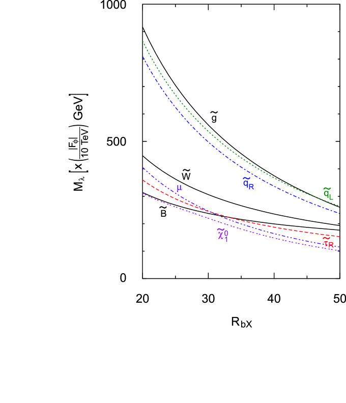
FIG. 3.: Typical sparticle masses at the electroweak scale for $n=1$ moduli. We assume the universal Kähler terms for visible and hidden sector fields; that is, $l={}^{\forall}m_{i}=1/3$ in Eq. (54). The horizontal axis denotes the ratio of two $F$-term contributions: $R_{bX}\equiv F_{\phi}/(F_{X}/2X_{R})$. In the figure, $\tan\beta=10$, and $F_{\phi}$ is fixed to be 20 TeV as an example, but the spectrum is scaled by $F_{\phi}$. The gaugino masses are given by the solid (black) lines, and the two-dotted-dashed line is the higgsino mass parameter $\mu$. We show the mass of the lightest neutralino ($\tilde{\chi}^{0}_{1}$) by two-dotted line. The dotted (green) and dotted-dashed (blue) lines represent left- and right-handed squarks of the first two generations, respectively. We show, in particular, the mass of right-handed scalar tau by dashed (red) line, which is the lightest among sfermions.

FIG. 4.: Constant contours of the mass of the lightest neutral Higgs boson for $n=1$ moduli. We assume the universal Kähler terms for visible and hidden sector fields; that is, $l={}^{\forall}m_{i}=1/3$ in Eq. (54). The dotted-dashed line denotes the current experimental bound from LEP II. In the figure, we take $\tan\beta=10$ and the top quark pole mass $M_{t}=178$ GeV.

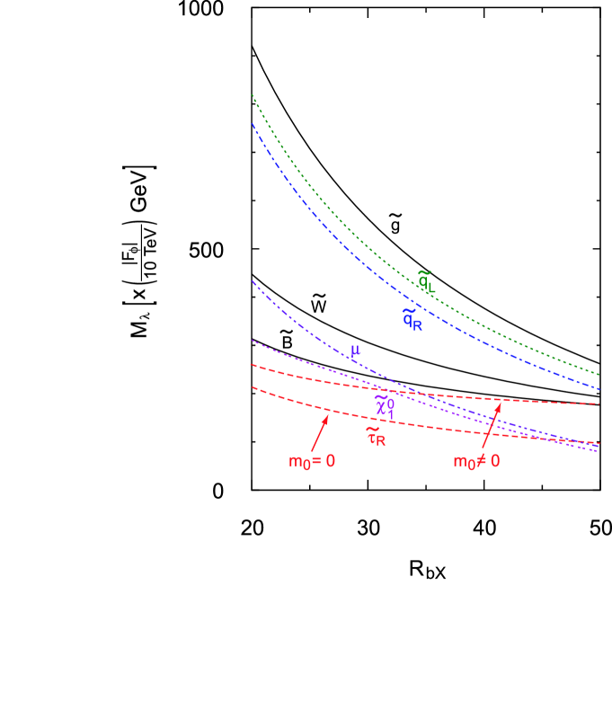
FIG. 5.: Typical sparticle masses at the electroweak scale for $n=3$ moduli. We assume the sequestered Kähler potential for visible and hidden sector fields; that is, $l={}^{\forall}m_{i}=0$ in Eq. (54). The horizontal axis denotes the ratio of two $F$-term contributions: $R_{bX}\equiv F_{\phi}/(F_{X}/2X_{R})$. In the figure, $\tan\beta=10$, and $F_{\phi}$ is fixed to be 20 TeV as an example, but the spectrum is scaled by $F_{\phi}$. The gaugino masses are given by the solid (black) lines, and the two-dotted-dashed line is the higgsino mass parameter $\mu$. We show the mass of the lightest neutralino ($\tilde{\chi}^{0}_{1}$) by two-dotted line. The dotted (green) and dotted-dashed (blue) lines represent left- and right-handed squarks of the first two generations, respectively. We show, in particular, the mass of right-handed scalar tau by dashed (red) lines, which is the lightest supersymmetric particle in a wide range of parameter space for vanishing universal corrections to scalar masses ($m_{0}=0$). Also shown is the mass of right-handed scalar tau for $m_{0}=1.5\times 10^{-2}|F_{\phi}|$.

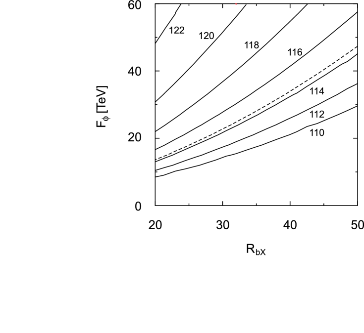
FIG. 6.: Constant contours of the mass of the lightest neutral Higgs boson for $n=3$ moduli. We assume the sequestered Kähler potential for visible and hidden sector fields; that is, $l={}^{\forall}m_{i}=0$ in Eq. (54). The dotted-dashed line denotes the current experimental bound from LEP II. In the figure, we take $\tan\beta=10$ and the top quark pole mass $M_{t}=178$ GeV. We here include the universal $m_{0}$ corrections to sfermion masses to avoid the stable scalar tau ($m_{0}=1.5\times 10^{-2}|F_{\phi}|$).

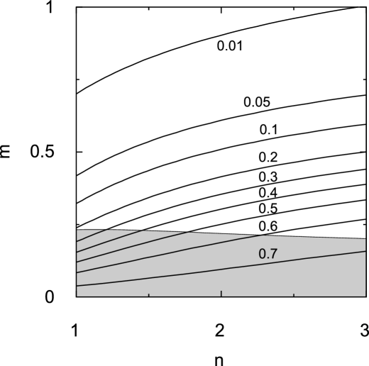
FIG. 7.: Constant contours of the higgsino composition $Z_{h}^{2}$ in the lightest neutralino. Here $m$ denotes the universal violation of sequestering between moduli and matter fields; $l={}^{\forall}m_{i}\equiv m$. Also shown is the shadow region in which the scalar tau is lighter than the lightest neutralino, and thus cosmologically disfavored. In the figure, $\tan\beta=10$ and $F_{\phi}=20$ TeV are assumed. A larger value of $F_{\phi}$ more increase the higgsino composition.

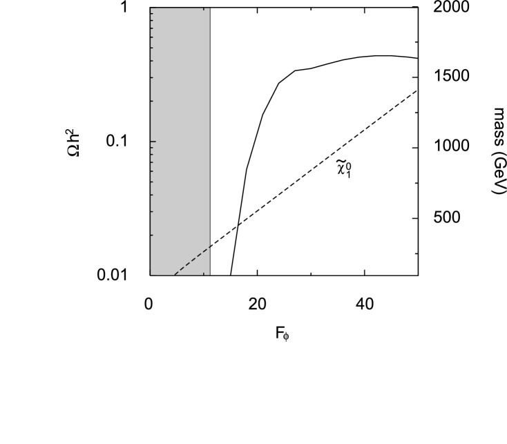
FIG. 8.: Thermal relic density of the lightest supersymmetric particle for $n=1$ moduli and $l={}^{\forall}m_{i}=1/3$. We take as an example $\tan\beta=10$ and $bX_{R}=35$. In the figure, we also plot the mass of the lightest neutralino. The shadow region in the left is excluded from the current experimental mass bound on the lightest Higgs boson.

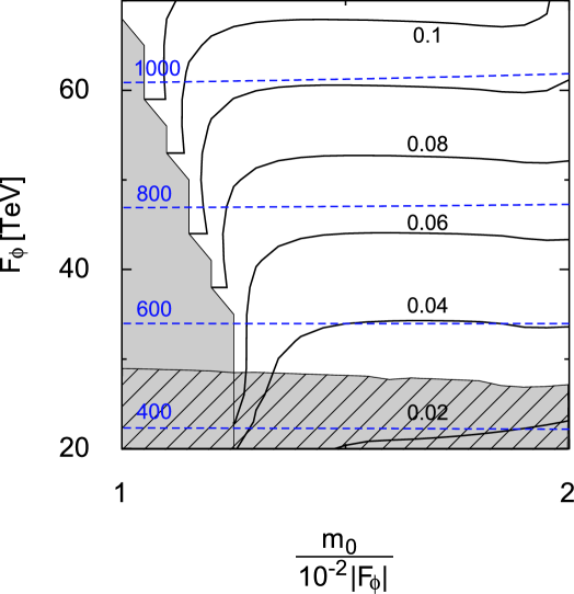
FIG. 9.: Thermal relic density of the lightest supersymmetric particle for $n=3$ moduli and $l={}^{\forall}m_{i}=0$. The solid lines are the contours of the abundance, and the dashed blue ones denote the mass of the lightest neutralino. We here introduce the universal scalar mass correction $m_{0}$, and take as an example $\tan\beta=10$ and $bX_{R}=35$. The shaded region in the left is excluded as the scalar tau being the lightest superparticle, and the shadow region in the bottom is also experimentally disfavored from the lightest Higgs boson mass.

FIG. 10.: The global structure of the moduli potential. Here we take $n=1$ and $l=1/3$. Above: the moduli potential at zero temperature. Below: the same potential at the critical temperature.

- [1] H.P. Nilles, Phys. Rept. 110 (1984) 1.
- [2] L. Girardello and M.T. Grisaru, Nucl. Phys. B194 (1982) 65.
- [3] E. Witten, Phys. Lett. B105 (1981) 267.
- [4] S. Dimopoulos and H. Georgi, Nucl. Phys. B193 (1981) 150; J.R. Ellis and D.V. Nanopoulos, Phys. Lett. B110 (1982) 44; J.F. Donoghue, H.P. Nilles and D. Wyler, Phys. Lett. B128 (1983) 55; L.J. Hall, V.A. Kostelecky and S. Raby, Nucl. Phys. B267 (1986) 415; F. Gabbiani and A. Masiero, Nucl. Phys. B322 (1989) 235; J.S. Hagelin, S. Kelley and T. Tanaka, Nucl. Phys. B415 (1994) 293; F. Gabbiani, E. Gabrielli, A. Masiero and L. Silvestrini, Nucl. Phys. B477 (1996) 321 [arXiv:hep-ph/9604387].
- [5] J.R. Ellis, S. Ferrara and D.V. Nanopoulos, Phys. Lett. B114 (1982) 231; W. Buchmuller and D. Wyler, Phys. Lett. B121 (1983) 321; J. Polchinski and M.B. Wise, Phys. Lett. B125 (1983) 393; M. Dugan, B. Grinstein and L.J. Hall, Nucl. Phys. B255 (1985) 413; T. Ibrahim and P. Nath, Phys. Rev. D57 (1998) 478 [arXiv:hep-ph/9708456]; S. Abel, S. Khalil and O. Lebedev, Nucl. Phys. B606 (2001) 151 [arXiv:hep-ph/0103320].
- [6] W. Buchmuller, K. Hamaguchi, M. Ratz and T. Yanagida, Phys. Lett. B588 (2004) 90 [arXiv:hep-ph/0402179]; J.L. Feng, S. Su and F. Takayama, Phys. Rev. D70 (2004) 075019 [arXiv:hep-ph/0404231].
- [7] S. Weinberg, Phys. Rev. Lett. 48 (1982) 1303.
- [8] H. Pagels and J.R. Primack, Phys. Rev. Lett. 48 (1982) 223.
- [9] T. Moroi, H. Murayama and M. Yamaguchi, Phys. Lett. B303 (1993) 289.
- [10] D. Lindley, Astrophys. J. 294 (1985) 1; M.Y. Khlopov and A.D. Linde, Phys. Lett. B138 (1984) 265; F. Balestra et al., Sov. J. Nucl. Phys. 39 (1984) 626; J.R. Ellis, J.E. Kim and D.V. Nanopoulos, Phys. Lett. B145 (1984) 181; R. Juszkiewicz, J. Silk and A. Stebbins, Phys. Lett. B158 (1985) 463; J.R. Ellis, D.V. Nanopoulos and S. Sarkar, Nucl. Phys. B259 (1985) 175; J. Audouze, D. Lindley and J. Silk, Astrophys. J. 293 (1985) L53; D. Lindley, Phys. Lett. B171 (1986) 235; M. Kawasaki and K. Sato, Phys. Lett. B189 (1987) 23; R.J. Scherrer and M.S. Turner, Astrophys. J. 331 (1988) 19; J.R. Ellis et al., Nucl. Phys. B373 (1992) 399; M.Yu. Khlopov et al., Phys. Atom. Nucl. 57 (1994) 1393; M. Kawasaki and T. Moroi, Prog. Theor. Phys. 93 (1995) 879 [arXiv:hep-ph/9403364]; Astrophys. J. 452 (1995) 506 [arXiv:astro-ph/9412055]; E. Holtmann, M. Kawasaki, K. Kohri and T. Moroi, Phys. Rev. D60 (1999) 023506 [arXiv:hep-ph/9805405].
- [11] K. Jedamzik, Phys. Rev. Lett. 84 (2000) 3248 [arXiv:astro-ph/9909445]; M. Kawasaki, K. Kohri and T. Moroi, Phys. Rev. D63 (2001) 103502 [arXiv:hep-ph/0012279]; R.H. Cyburt, J.R. Ellis, B.D. Fields and K.A. Olive, Phys. Rev. D67 (2003) 103521 [arXiv:astro-ph/0211258].
- [12] K. Kohri, Phys. Rev. D64 (2001) 043515 [arXiv:astro-ph/0103411]; K. Kohri and J. Yokoyama, Phys. Rev. D61 (2000) 023501 [arXiv:astro-ph/9908160].
- [13] M. Kawasaki, K. Kohri and T. Moroi, arXiv:astro-ph/0402490; Phys. Rev. D71 (2005) 083502 [arXiv:astro-ph/0408426].
- [14] G.D. Coughlan, W. Fischler, E.W. Kolb, S. Raby and G.G. Ross, Phys. Lett. B131 (1983) 59; B. de Carlos, J.A. Casas, F. Quevedo and E. Roulet, Phys. Lett. B318 (1993) 447 [arXiv:hep-ph/9308325]; T. Banks, D.B. Kaplan and A.E. Nelson, Phys. Rev. D49 (1994) 779 [arXiv:hep-ph/9308292].
- [15] J.R. Ellis, D.V. Nanopoulos and M. Quiros, Phys. Lett. B174 (1986) 176.
- [16] T. Moroi, M. Yamaguchi and T. Yanagida, Phys. Lett. B342 (1995) 105 [arXiv:hep-ph/9409367].
- [17] L. Randall and S. Thomas, Nucl. Phys. B449 (1995) 229 [arXiv:hep-ph/9407248].
- [18] K. Kohri, M. Yamaguchi and J. Yokoyama, Phys. Rev. D70 (2004) 043522 [arXiv:hep-ph/0403043].
- [19] K. Kohri, M. Yamaguchi and J. Yokoyama, arXiv:hep-ph/0502211.
- [20] M. Dine, A.E. Nelson and Y. Shirman, Phys. Rev. D51 (1995) 1362 [arXiv:hep-ph/9408384]; M. Dine, A.E. Nelson, Y. Nir and Y. Shirman, Phys. Rev. D53 (1996) 2658 [arXiv:hep-ph/9507378]; G.F. Giudice and R. Rattazzi, Phys. Rept. 322 (1999) 419 [arXiv:hep-ph/9801271].
- [21] H.P. Nilles, Phys. Lett. B115 (1982) 193; S. Ferrara, L. Girardello and H.P. Nilles, Phys. Lett. B125 (1983) 457; T.R. Taylor, Phys. Lett. B164 (1985) 43; S. Ferrara, N. Magnoli, T.R. Taylor and G. Veneziano, Phys. Lett. B245 (1990) 409; P. Horava, Phys. Rev. D54 (1996) 7561 [arXiv:hep-th/9608019].
- [22] N.V. Krasnikov, Phys. Lett. B193 (1987) 37; T.R. Taylor, Phys. Lett. B252 (1990) 59; J.A. Casas, Z. Lalak, C. Munoz and G.G. Ross, Nucl. Phys. B347 (1990) 243; B. de Carlos, J.A. Casas and C. Munoz, Nucl. Phys. B399 (1993) 623 [arXiv:hep-th/9204012].
- [23] J.P. Derendinger, L.E. Ibanez and H.P. Nilles, Phys. Lett. B155 (1985) 65; Nucl. Phys. B267 (1986) 365; M. Dine, R. Rohm, N. Seiberg and E. Witten, Phys. Lett. B156 (1985) 55; A. Font, L.E. Ibanez, D. Lust and F. Quevedo, Phys. Lett. B245 (1990) 401; P. Binetruy and M.K. Gaillard, Phys. Lett. B253 (1991) 119; Z. Lalak, A. Niemeyer and H.P. Nilles, Nucl. Phys. B453 (1995) 100 [arXiv:hep-th/9503170].
- [24] T. Banks and M. Dine, Phys. Rev. D50 (1994) 7454 [arXiv:hep-th/9406132]; P. Binetruy, M.K. Gaillard and Y.Y. Wu, Nucl. Phys. B481 (1996) 109 [arXiv:hep-th/9605170]; T. Barreiro, B. de Carlos and E.J. Copeland, Phys. Rev. D57 (1998) 7354 [arXiv:hep-ph/9712443].
- [25] S.B. Giddings, S. Kachru and J. Polchinski, Phys. Rev. D66 (2002) 106006 [arXiv:hep-th/0105097]; S. Kachru, M.B. Schulz and S. Trivedi, JHEP 0310 (2003) 007 [arXiv:hep-th/0201028].
- [26] S. Kachru, R. Kallosh, A. Linde and S.P. Trivedi, Phys. Rev. D68 (2003) 046005 [arXiv:hep-th/0301240].
- [27] K. Choi, A. Falkowski, H.P. Nilles, M. Olechowski and S. Pokorski, JHEP 0411 (2004) 076 [arXiv:hep-th/0411066].
- [28] L. Randall and R. Sundrum, Nucl. Phys. B557 (1999) 79 [arXiv:hep-th/9810155]; G.F. Giudice, M.A. Luty, H. Murayama and R. Rattazzi, JHEP 9812 (1998) 027 [arXiv:hep-ph/9810442]; J.A. Bagger, T. Moroi and E. Poppitz, JHEP 0004 (2000) 009 [arXiv:hep-th/9911029].
- [29] M. Endo, M. Yamaguchi and K. Yoshioka, Phys. Lett. B586 (2004) 382 [arXiv:hep-ph/0311206].
- [30] M. Kaku, P.K. Townsend and P. van Nieuwenhuizen, Phys. Rev. D17 (1978) 3179; W. Siegel and S.J. Gates, Nucl. Phys. B147 (1979) 77; E. Cremmer, S. Ferrara, L. Girardello and A. Van Proeyen, Nucl. Phys. B212 (1983) 413; T. Kugo and S. Uehara, Nucl. Phys. B226 (1983) 49.
- [31] S. Weinberg and E. Witten, Phys. Lett. B96 (1980) 59.
- [32] K. Choi, Phys. Rev. Lett. 72 (1994) 1592 [arXiv:hep-ph/9311352].
- [33] R. Rohm and E. Witten, Annals Phys. 170 (1986) 454.
- [34] M.A. Luty and R. Sundrum, Phys. Rev. D62 (2000) 035008 [arXiv:hep-th/9910202].
- [35] S. Gukov, C. Vafa and E. Witten, Nucl. Phys. B584 (2000) 69 [Erratum-ibid. B608 (2001) 477] [arXiv:hep-th/9906070].
- [36] E. Witten, Nucl. Phys. B474 (1996) 343 [arXiv:hep-th/9604030]; S. Katz and C. Vafa, Nucl. Phys. B497 (1997) 196 [arXiv:hep-th/9611090]; M. Berg, M. Haack and B. Kors, Phys. Rev. D71 (2005) 026005 [arXiv:hep-th/0404087].
- [37] E.I. Buchbinder and B. A. Ovrut, Phys. Rev. D69 (2004) 086010 [arXiv:hep-th/0310112]; S. Gukov, S. Kachru, X. Liu and L. McAllister, Phys. Rev. D69 (2004) 086008 [arXiv:hep-th/0310159]; M. Becker, G. Curio and A. Krause, Nucl. Phys. B693 (2004) 223 [arXiv:hep-th/0403027]; G. Curio, A. Krause and D. Lust, arXiv:hep-th/0502168.
- [38] K. Becker, M. Becker, K. Dasgupta and P.S. Green, JHEP 0304 (2003) 007 [arXiv:hep-th/0301161]; G.L. Cardoso, G. Curio, G. Dall’Agata and D. Lust, JHEP 0310 (2003) 004 [arXiv:hep-th/0306088]; S. Gurrieri, A. Lukas and A. Micu, Phys. Rev. D70 (2004) 126009 [arXiv:hep-th/0408121].
- [39] R. Bousso and J. Polchinski, JHEP 0006 (2000) 006 [arXiv:hep-th/0004134]; J.L. Feng, J. March-Russell, S. Sethi and F. Wilczek, Nucl. Phys. B602 (2001) 307 [arXiv:hep-th/0005276]; L. Susskind, arXiv:hep-th/0302219; M.R. Douglas, JHEP 0305 (2003) 046 [arXiv:hep-th/0303194]; T. Banks, M. Dine and E. Gorbatov, JHEP 0408 (2004) 058 [arXiv:hep-th/0309170].
- [40] A. Falkowski, Z. Lalak and S. Pokorski, Nucl. Phys. B613 (2001) 189 [arXiv:hep-th/0102145]; M.A. Luty and R. Sundrum, Phys. Rev. D64 (2001) 065012 [arXiv:hep-th/0012158]; J. Bagger, D. Nemeschansky and R.J. Zhang, JHEP 0108 (2001) 057 [arXiv:hep-th/0012163]; D. Marti and A. Pomarol, Phys. Rev. D64 (2001) 105025 [arXiv:hep-th/0106256].
- [41] K. Inoue, M. Kawasaki, M. Yamaguchi and T. Yanagida, Phys. Rev. D45 (1992) 328.
- [42] A. Pomarol and R. Rattazzi, JHEP 9905 (1999) 013 [arXiv:hep-ph/9903448]; E. Katz, Y. Shadmi and Y. Shirman, JHEP 9908 (1999) 015 [arXiv:hep-ph/9906296]; M. Yamaguchi and K. Yoshioka, Phys. Lett. B543 (2002) 189 [arXiv:hep-ph/0204293].
- [43] L.E. Ibanez and D. Lust, Nucl. Phys. B382 (1992) 305 [arXiv:hep-th/9202046]; B. de Carlos, J.A. Casas and C. Munoz, Phys. Lett. B299 (1993) 234 [arXiv:hep-ph/9211266]; V.S. Kaplunovsky and J. Louis, Phys. Lett. B306 (1993) 269 [arXiv:hep-th/9303040]; A. Brignole, L.E. Ibanez and C. Munoz, Nucl. Phys. B422 (1994) 125 [Erratum-ibid. B436 (1995) 747] [arXiv:hep-ph/9308271]; T. Kobayashi, D. Suematsu, K. Yamada and Y. Yamagishi, Phys. Lett. B348 (1995) 402 [arXiv:hep-ph/9408322].
- [44] P.G. Camara, L.E. Ibanez and A.M. Uranga, Nucl. Phys. B689 (2004) 195 [arXiv:hep-th/0311241]; Nucl. Phys. B708 (2005) 268 [arXiv:hep-th/0408036]; D. Lust, S. Reffert and S. Stieberger, Nucl. Phys. B706 (2005) 3 [arXiv:hep-th/0406092]; arXiv:hep-th/0410074.
- [45] S. Eidelman et al. [Particle Data Group Collaboration], Phys. Lett. B592 (2004) 1.
- [46] Y. Okada, M. Yamaguchi and T. Yanagida, Prog. Theor. Phys. 85 (1991) 1; Phys. Lett. B262 (1991) 54; J.R. Ellis, G. Ridolfi and F. Zwirner, Phys. Lett. B257 (1991) 83; H.E. Haber and R. Hempfling, Phys. Rev. Lett. 66 (1991) 1815.
- [47] S. Komine and M. Yamaguchi, Phys. Rev. D63 (2001) 035005 [arXiv:hep-ph/0007327].
- [48] V.M. Abazov et al. [D0 Collaboration], Nature 429 (2004) 638 [arXiv:hep-ex/0406031].
- [49] J.L. Feng, K.T. Matchev and T. Moroi, Phys. Rev. Lett. 84 (2000) 2322 [arXiv:hep-ph/9908309]; Phys. Rev. D61 (2000) 075005 [arXiv:hep-ph/9909334].
- [50] S. Heinemeyer, W. Hollik and G. Weiglein, arXiv:hep-ph/0002213; M. Frank, S. Heinemeyer, W. Hollik and G. Weiglein, arXiv:hep-ph/0202166.
- [51] Y. Kawamura, H. Murayama and M. Yamaguchi, Phys. Rev. D51 (1995) 1337 [arXiv:hep-ph/9406245]; N. Polonsky and A. Pomarol, Phys. Rev. Lett. 73 (1994) 2292 [arXiv:hep-ph/9406224]; Phys. Rev. D51 (1995) 6532 [arXiv:hep-ph/9410231].
- [52] D.N. Spergel et al. [WMAP Collaboration], Astrophys. J. Suppl. 148 (2003) 175 [arXiv:astro-ph/0302209].
- [53] J.R. Ellis, K.A. Olive, Y. Santoso and V.C. Spanos, Phys. Lett. B565 (2003) 176 [arXiv:hep-ph/0303043]; U. Chattopadhyay, A. Corsetti and P. Nath, Phys. Rev. D68 (2003) 035005 [arXiv:hep-ph/0303201].
- [54] P. Gondolo et al., JCAP 0407 (2004) 008 [arXiv:astro-ph/0406204].
- [55] V. Bertin, E. Nezri and J. Orloff, JHEP 0302 (2003) 046 [arXiv:hep-ph/0210034]; A. Birkedal-Hansen and B.D. Nelson, Phys. Rev. D67 (2003) 095006 [arXiv:hep-ph/0211071]; U. Chattopadhyay and D.P. Roy, Phys. Rev. D68 (2003) 033010 [arXiv:hep-ph/0304108]; D.G. Cerdeno, E. Gabrielli, M.E. Gomez and C. Munoz, JHEP 0306 (2003) 030 [arXiv:hep-ph/0304115]; D.G. Cerdeno and C. Munoz, JHEP 0410 (2004) 015 [arXiv:hep-ph/0405057].
- [56] S. Kachru et al., JCAP 0310 (2003) 013 [arXiv:hep-th/0308055]; J.J. Blanco-Pillado et al., JHEP 0411 (2004) 063 [arXiv:hep-th/0406230]; R. Kallosh and A. Linde, JHEP 0412 (2004) 004 [arXiv:hep-th/0411011].
- [57] R. Brustein and P.J. Steinhardt, Phys. Lett. B302 (1993) 196 [arXiv:hep-th/9212049].
- [58] R. Brustein, S.P. de Alwis and P. Martens, Phys. Rev. D70 (2004) 126012 [arXiv:hep-th/0408160].
- [59] W. Buchmuller, K. Hamaguchi, O. Lebedev and M. Ratz, Nucl. Phys. B699 (2004) 292 [arXiv:hep-th/0404168]; JCAP 0501 (2005) 004 [arXiv:hep-th/0411109].
- [60] J.I. Kapusta, “Finite Temperature Field Theory,” Cambridge University Press, 1989.
- [61] G. Huey, P.J. Steinhardt, B.A. Ovrut and D. Waldram, Phys. Lett. B476 (2000) 379 [arXiv:hep-th/0001112]; W. Buchmuller, K. Hamaguchi and M. Ratz, Phys. Lett. B574 (2003) 156 [arXiv:hep-ph/0307181].
- [62] K. Choi, A. Falkowski, H.P. Nilles and M. Olechowski, Nucl. Phys. B718 (2005) 113 [arXiv:hep-th/0503216].