In the strongly correlated environment of high-temperature cuprate superconductors, the spin and charge degrees of freedom of an electron seem to separate from each other. A similar phenomenon may be present in the strong coupling phase of Yang-Mills theories, where a separation between the color charge and the spin of a gluon could play a role in a mass gap formation. Here we study the phase structure of a decomposed $SU(2)$ Yang-Mills theory in a mean field approximation, by inspecting quantum fluctuations in the condensate which is formed by the color charge component of the gluon field. Our results suggest that the decomposed theory has an involved phase structure. In particular, there appears to be a phase which is quite reminiscent of the superconducting phase in cuprates. We also find evidence that this phase is separated from the asymptotically free theory by an intermediate pseudogap phase.

Splitting The Gluon?

I Introduction

There seem to be some remarkable similarities between high-temperature cuprate superconductivity in condensed matter physics and the problem of mass gap in the Yang-Mills theory of particle physics. It appears that in both cases the basic theoretical problem is the same, the absence of a natural condensate to describe the symmetry breaking that takes place. In high-temperature superconductors electrons do not form conventional Cooper pairs and the standard BCS-description of superconductivity can not be applied in any obvious manner. There is no obvious alternative choice of condensate that leads to superconductivity. In a very similar way, in the case of Yang-Mills theories we do not have any natural candidate for a condensate of the correct dimension, that describes the mass gap of gluons. Could it then be that in both cases the condensate has a similar origin?

It is definitely worth some effort to try and apply similar techniques to both problems. One promising method in the context of high temperature superconductivity is the slave-boson description, which has been studied actively and1 ; bask ; lee . This approach is based on the curious idea that, in the strongly correlated environment of cuprate superconductors, the electron (or hole) is no longer a fundamental mode of excitation, and thus electronic modes do not behave like a structureless fundamental object. Instead the electron can be interpreted as a composite particle, constructed from two quasi-particles. One of these is described by a charge neutral, spin-$1/2$ fermionic operator $f_{i\sigma}$ where $i$ is the site label and $\sigma=\uparrow,\downarrow$ is the spin index. This operator corresponds to a particle called a spinon, and it carries the (statistical) spin degree of freedom of the electron. The other excitation is described by a spinless bosonic operator $b^{T}_{i}=(b_{i1},b_{i2})$. It corresponds to a particle which is called a holon and it carries the electric charge of the electron. In terms of these two operators, the electron operator $c_{i\sigma}$ decomposes as

$$c_{i\sigma}=\frac{1}{\sqrt{2}}b^{\dagger}_{i}\psi_{i\sigma}\quad,$$ (1)

where we have combined the spinon operators as

$$\psi^{T}_{i\sigma}=(f_{i\sigma},\epsilon_{\sigma\tilde{\sigma}}f^{\dagger}_{i\tilde{\sigma}})\quad.$$ (2)

The decomposition (1) also introduces an internal $U(1)$ gauge symmetry, since it is invariant under the simultaneous change-of-phase transformation

$$b_{i}\to e^{i\theta}b_{i},\qquad\psi_{i\sigma}\to e^{i\theta}\psi_{i\sigma}.$$ (3)

As a result we have a compact $U(1)$ gauge interaction between the spinon and holon. Under normal circumstances we expect that the strength of this $U(1)$ interaction increases with increasing energy, to the effect that at high energies the spinon and holon are confined into a (point-like) electron. But in a strongly correlated environment, such as in a cuprate superconductor, the spin and the charge of the electron can become independent excitations and1 ; bask ; lee . This leads to a rather involved phase diagram, with several different regions lee . One of the easiest ways to study the phase structure is using a mean-field theory. This is obtained by integrating over the fermions $\psi_{i\sigma}$, and one finds that ($d$-wave) superconductivity occurs when the remaining bosonic holon field $b_{i}$ condenses,

$$\langle b_{i}^{\dagger}b_{i}\rangle=\Delta_{b}\neq 0.$$ (4)

Of substantial interest is also the possibility that the system can enter a pseudogap phase. This is a precursor to the superconducting phase with the characteristic property that even though the underlying symmetry is broken, the effective bosonic order parameter $\Delta_{b}$ vanishes due to quantum fluctuations.

Curiously, a very similar picture seems to emerge in the case of a pure four dimensional $SU(2)$ Yang-Mills theory. In analogy to the slave-boson decomposition of an electron, the off-diagonal components of the non-abelian gluon field become composite particles, with a separation between their color-charge and spin degrees of freedom ludvig1 (see also oma1 ; ludvig2 ). Here we shall study the phase structure of the decomposed gauge theory, by following the mean-field approach to high-temperature superconductivity. We first construct a mean-field state where we integrate over the charge neutral spin degree of freedom of the off-diagonal gluon. We propose that in the strong coupling regime the spinless color-charge carrier of the gluon becomes condensed. The ensuing phase is analogous to the superconducting phase in cuprates. Furthermore, in analogy with cuprate superconductors we also find evidence that there is an intermediate pseudogap phase, a cross-over region between the superconducting-like phase and the asymptotically-free deconfined limit of the Yang-Mills theory.

II Slave-Boson Decomposition In Yang-Mills

The slave-boson decomposition of the $SU(2)$ gauge field $A^{a}_{\mu}$ ($a=1,2,3$ and $\mu=0,1,2,3$) proceeds as follows ludvig1 ; oma1 : We first separate the diagonal Cartan component $A^{3}_{\mu}=A_{\mu}$ from the off-diagonal components $A^{1,2}_{\mu}$, and combine the latter into the complex field $W_{\mu}=A^{1}_{\mu}+iA^{2}_{\mu}$. We then introduce a complex vector field ${\bm{e}}_{\mu}$ with

$${\bm{e}}_{\mu}{\bm{e}}_{\mu}=0\qquad\text{and}\qquad{\bm{e}}_{\mu}{\bm{e}}^{*}_{\mu}=1.$$

We also introduce two spinless complex scalar fields $\psi_{1}$ and $\psi_{2}$. The ensuing decomposition of $W_{\mu}$ is ludvig1

$$W_{\mu}=A^{1}_{\mu}+iA^{2}_{\mu}=\psi_{1}{\bm{e}}_{\mu}+\psi_{2}^{*}{\bm{e}}^{*}_{\mu}.$$ (5)

This is clearly a direct analogue of Eq. (1), a decomposition of $W_{\mu}$ into spinless bosonic scalars $\psi_{1,2}$ which describe the gluonic holons that carry the color charge of the $W_{\mu}$, and a color-neutral spin-one vector ${\bm{e}}_{\mu}$ which is the gluonic spinon that carries the statistical spin degrees of freedom of $W_{\mu}$.

In general, the present gluonic slave-boson decomposition is not gauge invariant. But in a proper gauge it can be given a gauge invariant meaning and in particular the combination

$$\rho^{2}=\rho_{1}^{2}+\rho_{2}^{2}=\langle|\psi_{1}|^{2}\rangle+\langle|\psi_{2}|^{2}\rangle$$ (6)

of the gluonic holons becomes a gauge invariant quantity. For this we introduce zakharov ; oma1

$$\int\rho^{2}=\int(\rho_{1}^{2}+\rho_{2}^{2})=\int\left[(A_{\mu}^{1})^{2}+(A_{\mu}^{2})^{2}\right]=\int W_{\mu}W_{\mu}^{*}.$$ (7)

This is in general gauge dependent. But if we consider the gauge orbit extrema of (7) with respect to the full $SU(2)$ gauge transformations, these extrema are by construction gauge independent quantities. Moreover, the gauge orbit extrema of (7) correspond to field configurations $W_{\mu}$ which are subject to a background version of the maximal abelian gauge oma1 ,

$$(\partial_{\mu}+igA_{\mu})W_{\mu}=0,$$ (8)

which is widely used in lattice studies hay . In the sequel we shall assume that the gauge fixing condition (8) has been implemented. The slave-boson decomposition then acquires a gauge invariant meaning, and in particular the condensate (6) is a gauge invariant quantity.

As in (3), the decomposition (5) remains intact when we change phases according to

$$\psi_{1,2}\to e^{i\theta}\psi_{1,2}\quad\text{and}\quad{\bm{e}}_{\mu}\to e^{-i\theta}{\bm{e}}_{\mu}.$$ (9)

This determines an internal compact $U(1)$ gauge structure. A compact $U(1)$ gauge theory is known to be confining when the coupling is sufficiently strong polyakov . The confining phase is separated by a first order phase transition from the deconfined weak coupling phase. Furthermore, since the running of the $\beta$-function of the compact $U(1)$ leads to an increase of the coupling with increasing energy, we expect that at high energy the gluonic holon and spinon become confined by an increasingly strong compact $U(1)$ interaction to the effect that the high energy Yang-Mills theory describes asymptotically free and pointlike gluons, as it should.

But at low energy and in a strongly correlated environment, maybe in the interior of hadronic particles, the internal $U(1)$ gauge interaction (9) can become weak and the spin and the color-charge degrees of freedom of the gluon can separate from each other. If in analogy with (4) the spinless color-carriers then condense

$$\rho^{2}=\rho_{1}^{2}+\rho_{2}^{2}=\langle\psi_{1}^{\dagger}\psi_{1}\rangle+\langle\psi_{2}^{\dagger}\psi_{2}\rangle=\Delta_{\psi}\not=0\quad,$$

we have a mass gap and the theory is in a phase which is very similar to the holon condensation phase of cuprate superconductors.

In the case of high-temperature superconductivity the basic criterion for the validity of the slave-boson decomposition is a dynamic one: The decomposition can occur only if the ensuing Hamiltonian admits a natural interpretation in terms of the decomposed variables. In particular, in the relevant background the holon and spinon operators should indeed describe proper particle states. We propose that the same criterion can also be adopted to Yang-Mills theories. A decomposition of the gauge field $A^{a}_{\mu}$ in terms of other fields leads to a valid description of the phase structure, only if the decomposed action has a natural structure and particle interpretation in terms of the new variables. In the case of Eq. (5) this criterion turns out to be satisfied. If we write the Yang-Mills action in terms of the decomposed variables, it admits a natural interpretation as a two-gap abelian Higgs model oma1 . This suggests that the present Yang-Mills version of the slave-boson decomposition might actually identify the correct dynamical degrees of freedom that describe the non-perturbative phases of the theory.

III The Mean-Field Theory

In the case of cuprate superconductors, the phase structure can be investigated using a mean-field theory that emerges when the original theory is averaged over the electronic spinon field. We now proceed in an analogous manner, and average the $SU(2)$ Yang-Mills action both over the color-spinon ${\bm{e}}_{\mu}$ and the Cartan component $A_{\mu}$ of the gauge field. Since we are only interested in the phase structure of the ensuing mean-field theory, it is sufficient to consider the free energy in a London limit where the slave-boson condensates

$$\rho_{1,2}^{2}=\langle|\psi_{1,2}|^{2}\rangle$$

are spatially uniform.

The integration over $A_{\mu}$ and ${\bm{e}}_{\mu}$ can be performed in various different ways. Our starting point is the one-loop result of Ref. lisa , which yields for the (London limit) condensates the dimensionally transmutated free energy

$$F=\frac{1}{8}g^{2}(\rho_{1}^{2}-\rho_{2}^{2})^{2}\cdot\biggl{(}1+\frac{22}{3}\frac{g^{2}}{(4\pi)^{2}}\cdot\biggl{[}\ln\frac{|\rho_{1}^{2}-\rho_{2}^{2}|}{\Lambda^{2}}-\frac{25}{6}\biggr{]}\biggr{)}\quad.$$ (10)

Here $\Lambda$ is the renormalization scale and $g^{2}$ is the ($\Lambda$ dependent) coupling constant and a finite renormalization $\Lambda\to\bar{\Lambda}$ sends $g\to\bar{g}$ with the familiar relation

$$\bar{g}^{2}=\frac{g^{2}}{1+\frac{22}{3}\frac{g^{2}}{(4\pi)^{2}}\ln(\bar{\Lambda}/\Lambda)}\quad,$$ (11)

or in infinitesimal form

$$\Lambda\cdot\frac{dg}{d\Lambda}=\beta(g)=-\frac{22}{3}\frac{g^{3}}{(4\pi)^{2}}\quad.$$

The minima of (10) are highly nondegenerate, and located on the $\rho_{1}>0$, $\rho_{2}>0$ branch of the hyperbola

$$|\rho_{1}^{2}-\rho_{2}^{2}|_{\text{min}}=\Lambda^{2}\exp\biggl{(}-\frac{24\pi^{2}}{11g^{2}}+\frac{11}{3}\biggr{)}\quad.$$ (12)

Along these hyperbola, the value of the free energy is

$$F_{\text{min}}=-\frac{11}{24}\frac{g^{4}}{16\pi^{2}}\Lambda^{4}\exp\biggl{(}-\frac{48\pi^{2}}{11g^{2}}+\frac{22}{3}\biggr{)}\quad.$$ (13)

Since (10) is a one-loop approximation it can not be used for providing numerically accurate predictions. For this, high-precision Monte Carlo simulations are needed. But if one is only interested in the qualitative features of the phase diagram, the explicit form (10) is adequate, as shown below.

Indeed, if we assume that the Yang-Mills $\beta$-function has no zeroes so that

$$\int\frac{dx}{\beta(x)}<0\quad,$$

the minimum values (12) and (13) can be represented in the renormalization group invariant form

$$(\rho_{1}^{2}-\rho_{2}^{2})^{2}_{\text{min}}=\Lambda^{4}\exp\biggl{(}-4\int\limits^{g}\frac{dx}{\beta(x)}+\frac{22}{3}\biggr{)},$$

and

$$F_{\text{min}}=-4\Lambda^{4}\cdot\int\limits^{g}\beta(x)dx\cdot\exp\biggl{(}-4\int\limits^{g}\frac{dx}{\beta(x)}+\frac{22}{3}\biggr{)}=-4\int\limits^{g}\beta(x)dx\cdot(\rho_{1}^{2}-\rho_{2}^{2})^{2}_{\text{min}}.$$

Consequently we expect that the qualitative features of our conclusions have a validity which extends beyond the one-loop level. For the present purposes it is sufficient to start from the notationally simpler version

$$\tilde{F}=\frac{1}{2}(\rho_{1}^{2}-\rho_{2}^{2})^{2}\cdot\biggl{(}1+\tilde{\lambda}\cdot\biggl{[}\ln\frac{|\rho_{1}^{2}-\rho_{2}^{2}|}{\Lambda^{2}}-\alpha\biggr{]}\biggr{)}\quad.$$ (14)

We normalize $F$ with the factor $(1-\lambda\alpha)$, set $\Lambda^{2}=1$ and redefine

$$\lambda=\frac{1}{2}\frac{\tilde{\lambda}}{1-\tilde{\lambda}\alpha}\quad,$$

and arrive at the final version of the free energy that we shall use in our analysis:

$$F=\frac{1}{2}(\rho_{1}^{2}-\rho_{2}^{2})^{2}\cdot\biggl{(}1+\lambda\cdot\ln(\rho_{1}^{2}-\rho_{2}^{2})^{2}\biggr{)}\quad.$$ (15)

In figure 1 we have plotted this free energy for $\lambda=100$, on the entire $(\rho_{1},\rho_{2})$ plane. The generic features of this potential, a ridge along the lines $\rho_{1}=\pm\rho_{2}$, and a narrow hyperbolic valley on both sides of these lines, are independent of $\lambda$, but the depth of the valleys and steepness of the potential are more prominent for larger values of $\lambda$, as used here.

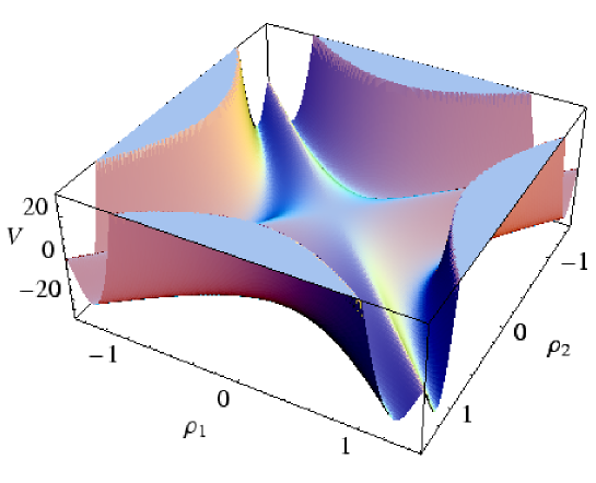
Figure 1: The free energy $F$ in equation (15), for $\lambda=100$. The physical branch corresponds to the quadrant $\rho_{1,2}\geq 0$. [color online.]

The Landau pole at

$$\tilde{\lambda}=1/\alpha$$ (16)

separates the strong coupling region with $\tilde{\lambda}>1/\alpha$ from the weak coupling region with $\tilde{\lambda}<1/\alpha$. Since the latter region includes the small coupling limit of the original Yang-Mills theory and since the free energy (10) can only be reliable for weak coupling, we shall in the following concentrate on the region $0\leq\tilde{\lambda}\leq{1}/{\alpha}.$ Notice that in terms of the redefined coupling $\lambda$ in (15), this corresponds to the region of a positive $\lambda$. In particular, if $\alpha$ in (14) is large, the strong coupling limit $\lambda\to\infty$ in (15), does not necessarily correspond to a strong coupling limit of the original model (14).

IV Classical Aspects

We first consider the properties of the free energy (15) at a classical level, where we do not include the quantum fluctuations in the spatially uniform London limit condensates $\rho_{1,2}$. This free energy has the following classical scaling symmetry martin ,

$$\rho^{\prime} = \frac{\rho}{c}\quad,$$

$$\lambda^{\prime} = \frac{\lambda}{1+2\lambda\ln(c^{2})}\quad,$$

$$F^{\prime} = \frac{1}{c^{4}}\cdot\frac{F}{1+2\lambda\ln c^{2}}\quad.$$ (17)

We can employ this scaling symmetry to restore the parameter $\Lambda$ in the free energy; see (14), (15). Indeed, it is obvious that this scaling symmetry reflects the renormalization group symmetry of the original Yang-Mills theory, with the scaling transformation of the coupling constant $\lambda$ a version of (11).

In addition, as a function on the entire $(\rho_{1},\rho_{2})$ plane the free energy has a discrete symmetry since it only depends depends on a polynomial combination of the condensates

$$F(\rho_{1},\rho_{2})=f\left((\rho_{1}^{2}-\rho_{2}^{2})^{2}\right).$$

and in addition we also have the gauge invariant polynomial combination in Eq. (7),

$$\rho^{2}=\rho_{1}^{2}+\rho_{2}^{2}\quad.$$ (18)

We are interested in linear transformations that act on the $(\rho_{1},\rho_{2})$ plane and leave both polynomials intact. These polynomials are exactly the basic invariants that generate the octonic dihedral group $D_{4}$ (also called $4mm$), which is the nonabelian symmetry group of the square.

The four branches of the hyperbola that minimize (15),

$$(\rho_{1}^{2}-\rho_{2}^{2})^{2}=\exp\left(\frac{1-\lambda}{\lambda}\right)\quad,$$ (19)

are separated by (non-analytic) ridges along the lines $\rho_{1}=\pm\rho_{2}$, and mapped to each other by the $D_{4}$ transformations. At the minima along the hyperbolic valleys the free energy is given by

$$E_{\text{min}}=-\frac{1}{2}\exp\left(\frac{1-\lambda}{\lambda}\right)\quad.$$ (20)

This ground state is highly degenerate, but the combination on the left-hand side of (19) is not the proper gauge invariant condensate. The gauge invariant condensate is given by Eq. (18), and we can employ it to remove the infinite degeneracy of the hyperbolic vacuum:

From (19) we conclude that the ground state value $\rho^{2}=v^{2}$ of the gauge invariant condensate (18) is bounded from below by a non-vanishing quantity,

$$\rho^{2}=\rho_{1}^{2}+\rho_{2}^{2}=v^{2}\geq|\rho_{1}^{2}-\rho_{2}^{2}|=\exp\left(\frac{1-\lambda}{2\lambda}\right).$$ (21)

When $v^{2}$ is larger than the lower bound in (21), there are eight solutions $(\rho_{1},\rho_{2})$ to the equations that define the vacuum

$$\rho_{1}^{2}+\rho_{2}^{2} = v^{2}\quad,$$

$$\rho_{1}^{2}-\rho_{2}^{2} = \pm\exp\left(\frac{1-\lambda}{2\lambda}\right)\quad.$$ (22)

But when $v^{2}$ coincides with the lower bound there are only four solutions,

$$\rho_{1}=\pm v\quad \& \quad\rho_{2}=0\quad,$$

$$\rho_{1}=0\quad \& \quad\rho_{2}=\pm v\quad.$$ (23)

which correspond to the vertices of the hyperbola. The solutions are mapped onto each other by the dihedral group $D_{4}$, and selecting any one as the ground state breaks the $D_{4}$ symmetry.

The solutions of (22) describe the generic situation where both condensates are non-vanishing. The solutions are $D_{4}$-degenerate, but we remove this degeneracy when we select the (physical) $\rho_{1,2}\geq 0$ quadrant. The remaining ground state is doubly degenerate under exchange of $\rho_{1}$ and $\rho_{2}$, which correspond to the physical scenario that in general the London limit densities are unequal.

Finally, the degenerate solutions (23) correspond to the limit where one of the two condensates vanishes, and again by selecting the physical quadrant $\rho_{1,2}\geq 0$ we remove the degeneracy.

According to (21) the ground state value of (18) is non-vanishing for all non-vanishing values of the coupling constant $\lambda$. This suggests that in the Yang-Mills theory the gauge invariant condensate (6) is also nonvanishing for all non-vanishing values of the coupling constant. This would mean that the mass gap in the Yang-Mills theory is present for all values of the coupling, and it vanishes only asymptotically in the short distance limit where the gluons become asymptotically free and massless.

V Quantum Mechanics - Numerical Approach

The classical treatment of the mean-field theory in the previous section suggests that the condensate (6) is always non-vanishing, hence a mass gap is present for all nontrivial values of the coupling. We now want to inspect what effects spatially homogeneous quantum fluctuations around the classical mean-field value have on this condensate. For this we need to improve the free energy so that it also includes the contribution from the momenta $\pi_{1,2}$ that are canonically conjugate to the (spatially homogeneous) condensates $\rho_{1,2}$. For computational simplicity we consider these condensates to be defined over the entire $(\rho_{1},\rho_{2})$ plane. This results in a $D_{4}$ symmetry, and by selecting the physically relevant values $\rho_{1,2}\geq 0$ for the condensates we then break this discrete symmetry.

The conjugate momenta are the generators of spatially homogeneous translations. Their inertia is undefined, and we therefore add a parameter $M$. The improved free energy can be interpreted as a Hamiltonian

$$H=\frac{1}{2M}\left(\pi_{1}^{2}+\pi_{2}^{2}\right)+\frac{1}{2}\left(\rho_{1}^{2}-\rho_{2}^{2}\right)^{2}\left(1+\lambda\ln\left(\rho_{1}^{2}-\rho_{2}^{2}\right)^{2}\right)\quad.$$ (24)

It corresponds to the effective action

$$S_{\text{eff}}=\int\limits_{0}^{T}dt\bigl{(}\pi_{1}\dot{\rho}_{1}+\pi_{2}\dot{\rho}_{2}-H[\pi,\rho]\bigr{)}\quad,$$ (25)

and the equations of motion for $S_{\text{eff}}$ are invariant under the following extension martin of the scaling transformation (17)

$$\rho^{\prime} = \frac{\rho}{c}\quad,$$

$$\pi^{\prime} = \sqrt{\frac{1}{1+2\lambda\ln(c^{2})}}\hskip 1.70717pt\frac{\pi}{c^{2}}\quad,$$

$$\lambda^{\prime} = \frac{\lambda}{1+2\lambda\ln(c^{2})}\quad,$$

$$t^{\prime} = \sqrt{1+2\lambda\ln(c^{2})}\cdot ct\quad.$$ (26)

We also note that the action (25) is clearly invariant under the dihedral $D_{4}$ symmetry group.

In order to study the effects of quantum fluctuations in the condensates we investigate the solutions of Schrödinger equation

$$-\frac{\hbar^{2}}{2M}\left(\partial_{1}^{2}+\partial_{2}^{2}\right)\psi(\rho_{1},\rho_{2})+\frac{1}{2}\left(\rho_{1}^{2}-\rho_{2}^{2}\right)^{2}\left(1+\lambda\ln\left(\rho_{1}^{2}-\rho_{2}^{2}\right)^{2}\right)\psi(\rho_{1},\rho_{2})=E\psi(\rho_{1},\rho_{2}).$$ (27)

We have studied this Schrödinger equation (27) numerically, using a highly-accurate finite difference approximation, on grids of varying size and spacing, using up to $400\times 400$ grid points. We have analyzed both the ground-state wave function and several of the low-lying excited-state wave functions when the coupling constant $\lambda$ in (27) varies for fixed $M$. According to the relation between (14) and (15), this surveys the phase structure of the theory at couplings below the Landau pole.

We note that since the Schrödinger equation (27) is invariant under the action of the dihedral $D_{4}$, the wave functions can be chosen to have definite $D_{4}$ transformation properties. Unfortunately, most discussions of point groups, see e.g. Butler , look for representations in 3D space, where one can distinguish between the groups $C_{4v}$ and $D_{4}$, but these groups act identically in the $xy$ plane. Following Mulliken’s ($A,B$ 1D irrep; $E$ 2D irrep) or Koster’s notation ($\Gamma_{i}$) as discussed in Ref. Butler , we have five possible representations of this group in two dimensions, see table 1.

Table 1: Character table (trace over classes of elements of the representation matrices) for $D_{4}$. The five classes on the top line are, respectively: $E$ identity; $2C_{4z}$ rotations over $\pm\pi/2$ around the $z$-axis; $C_{2z}$ a rotation over $\pi$ around the $z$-axis; $2\sigma_{y}$ reflections in the $x$ or $y$-axis; $2\sigma_{xy}$ reflections in the lines $x=\pm y$.

$\displaystyle\begin{array}[]{lrrrrrlll}&E&2C_{4z}&C_{2z}&2\sigma_{y}&2\sigma_{xy}&\text{representative wave function}\\ \hline\cr A_{1}=\Gamma_{1}&1&1&1&1&1&f(x^{2}+y^{2})\\ A_{2}=\Gamma_{2}&1&1&1&-1&-1&xy(x^{2}-y^{2})\\ B_{1}=\Gamma_{3}&1&-1&1&1&-1&x^{2}-y^{2}\\ B_{2}=\Gamma_{4}&1&-1&1&-1&1&xy\\ E=\Gamma_{5}&2&0&-2&0&0&(x,y)\text{ and }(x+y,x-y)\\ \end{array}$

In that table we have also listed representative wave functions for all the irreps. Looking at the symmetry of the wave functions, we expect $A_{1}$, $B_{1}$ and one of the $E$ cases with zeroes on the lines $x=\pm y$ to form four almost degenerate states as $\lambda$ grows large, as borne out by figure 5 below.

When $\lambda\to 0$ the Schrödinger equation (27) reduces to the $x^{2}y^{2}$ model which has been studied in detail in simon . In particular, it has been established that the spectrum of the $x^{2}y^{2}$ model is discrete, the eigenstates are normalizable, and the ground state energy is separated from $E=0$ by a non-vanishing gap.

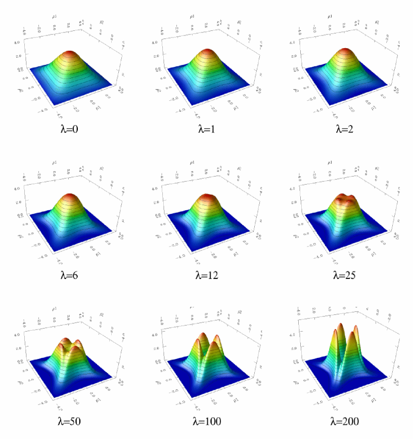
Figure 2: The ground state wave function for $\lambda$ from $0$ to $200$. A result for a larger value of $\lambda$ is given in figure 5. [color online.]

In figure 2 we depict the behavior of the numerically constructed ground state wave function for different values of $\lambda$ for $M=1$. Very similar behavior is found for other values of $M$, but as analyzed in more detail below, the similarity is greatest if we compare solutions for identical values of $\lambda M$. We find that the wave function exhibits three different kinds of qualitative behavior. There is a weak coupling region $0<\lambda M<\lambda_{a}\approx 10$, an intermediate coupling region $\lambda_{a}<\lambda M<\lambda_{b}\approx 500$ and a strong coupling region $\lambda_{b}<\lambda$. In all cases the ground-state wave function lies in the lowest symmetric representation ($A_{1}$) of $D_{4}$. These regions have the following characteristic features:

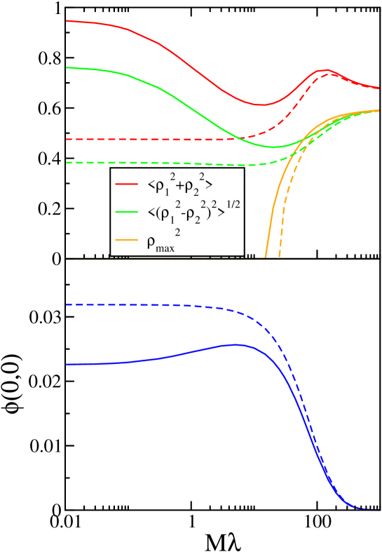
Figure 3: The upper panel shows the two condensates $\rho^{2}$ and $((\rho_{1}^{2}-\rho_{2}^{2})^{2})^{1/2}$ , and the distance of the maximum value of the ground state wave function to the origin. The lower panel gives the value of the ground state wave function at the origin. The solid lines show the values for $M=1$, and the dashed lines for the larger value $M=8$. [color online.]

Weak coupling:

In the weak coupling region with $M\lambda<\lambda_{a}\approx 10$, we find that the ground state wave function is qualitatively reminiscent of the ground state wave function in the $x^{2}y^{2}$ model, in particular it has a single maximum which is located at the origin of the $(\rho_{1},\rho_{2})$ plane. We also find that the value of the wave function at its maximum varies very slowly as a function of $\lambda$, especially for a large value of $M$, which means a more tightly localized wave function, see figure (3); Both the shape of the ground state wave function and the location of its maximum suggest, that in this weak coupling region quantum fluctuations tend to restore the system towards the symmetric state $\rho^{2}\approx 0$ so that there would not be any mass gap in the underlying Yang-Mills theory.

Clearly, we find non-zero condensate values for any finite value of $M$. As suggested by figure 4, the condensate goes to zero at $\lambda=0$, as $M$ goes to infinity but there remains a cross-over to a broken phase at stronger coupling. This is consistent with the fact, that in the limit of vanishing coupling the Yang-Mills theory describes free massless gluons.

Independent of $M$, when $\lambda$ approaches $\lambda_{a}$ the value of $\rho_{\lambda}$ overshoots the classical value given by the right-hand side of (19). Consequently the expectation value (6) detects the presence of symmetry breaking and the ensuing nontriviality of the condensate, even though this is not reflected in the location of the maximum value of the ground state wave function.

Such a behavior where the condensate (6) detects a symmetry breaking while the wave function tends to retain the symmetry, is reminiscent of the pseudogap phase lee . As a consequence we propose that in the weak coupling region $0<\lambda<\lambda_{a}$ the underlying Yang-Mills theory is in a pseudogap phase, a cross-over region which terminates in the asymptotically free theory as $\lambda\to 0$. Presumably this region is intimately related to a Coulomb-like phase in the Yang-Mills theory.

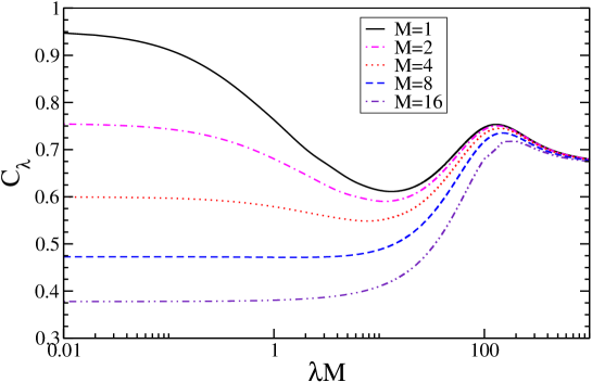
Figure 4: The condensate (6), as a function of $M\lambda$ for various values of $M$, as indicated in the plot. [color online.]

Intermediate coupling:

When $10\approx M\lambda_{a}<M\lambda<M\lambda_{b}\approx 500$ there is a clear qualitative change in the behavior of both the ground state wave function and the condensates (6). For these values of the coupling the origin in the $(\rho_{1},\rho_{2})$ plane becomes a local minimum, and instead there are now four maxima in the wave function. These maxima are all located the same distance $\rho_{\text{max}}$ from the origin, and related to each other by the $D_{4}$ symmetry. Both the value of the ground state wave function at the origin, and the condensate (6) decrease essentially linearly in the logarithmic scales of figure 3, while the value of $\rho_{\text{max}}$ very rapidly approaches the classical limiting value determined by (19), as $\lambda\to\lambda_{b}$. In particular, as $\lambda\to\lambda_{b}$ the value of the condensate (6) becomes less than its classical bound in (19), but is still clearly bounded from below.

In this intermediate coupling region both the ground state wave function and the condensate (6) behave similarly, and in a manner which suggests that the underlying Yang-Mills theory has a mass gap. Indeed, the behavior is quite reminiscent of the superconducting phase in cuprate superconductors. We find it natural to propose that this region of the coupling constant describes a superconducting mass-gap phase of the Yang-Mills theory, maybe a magnetic dual to the confinement phase.

Strong coupling:

When $\lambda\to\lambda_{b}\approx 1000$ we detect a new transition, towards a strong coupling regime $\lambda_{b}<\lambda$. Now the value of the ground state wave function essentially vanishes at the origin, see figure 3. The value of the condensate (6) again increases, and asymptotically approaches the value $\rho_{\text{max}}=\exp(-1/4)$ which is the classical $\lambda\to\infty$ lower bound value (21) for the minimum distance between the potential minimum and the origin. Indeed, for the entire strong coupling region $\lambda_{b}<\lambda$ we find that the difference between the classical and quantum values of the condensate is very small, suggesting that in this region one of the condensates essentially vanishes. Consequently as $\lambda\to\infty$ the system becomes driven towards a degenerate ground state where one of the condensates asymptotically vanishes, while the other becomes asymptotically determined by the classical theory.

The strong coupling region retains the major characteristics of the intermediate coupling region: There is a mass gap, and the ground state wave function is peaked at a nontrivial value of the condensate, even though in the infinite coupling limit one of the (quantum) condensates seems to vanishes asymptotically– it seems that the two quantities $\rho^{2}$ and $((\rho_{1}^{2}-\rho_{2}^{2})^{2})^{1/2}$ coincide as $\lambda\rightarrow\infty$. But in this region the ground state wave function has the additional characteristic property that it (essentially) vanishes in a neighborhood around the origin, thus becoming (essentially) separated into four disjoint components. This means that the lowest four states, consisting of two one-dimensional representations and one two-dimensional one, become degenerate. While we do recognize that in a finite dimensional quantum mechanical model there always remains a (vanishingly small) tail of the wave function at the origin, the numerically observed vanishing of the wave function in the vicinity of the origin is very definite. Consequently we envision, that in the underlying field theory with its infinite number of degrees of freedom, there is a true transition where the tunneling between the four dihedrally symmetric branches of the ground state wave function becomes totally suppressed.

Finally, we find that the at these high values of $\lambda$ the wave functions of the four lowest states become degenerate, see figures 5. The symmetries of these states correspond to $A_{1}$, $E$ and $B_{1}$ irreps, as argued above.

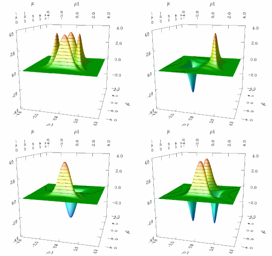
Figure 5: The four lowest eigenstates (from left to right and top to bottom) of the problem (27) for $\lambda=400$. [color online.]

VI Quantum Mechanics - Asymptotic Analysis

The present model is a generalization of the $x^{2}y^{2}$ model, a notoriously complex system simon . While the $\lambda\to 0$ limit of our numerical results reproduce the known properties of the $x^{2}y^{2}$ model, there is a need to confirm the main features of our $\lambda\not=0$ results by formal analysis. For this, we now consider the relevant asymptotic behavior of the ground state wave function.

VI.1 Large distance behavior of the wave function

For $\lambda=0$ the behavior of the solutions of (27) are known and have been discussed in detail in simon : The spectrum is discrete, the eigenstates are normalizable, and the ground state energy is separated from $E=0$ by a non-vanishing gap. Our numerical investigations suggest that these conclusions persist for non-vanishing values of $\lambda$. We now proceed to verify this using asymptotic analysis of the Schrödinger equation (27). In particular, we wish to establish that the wave function is indeed normalizable.

When $\rho_{1}\not=\pm\rho_{2}$ the potential in (27) is bounded from below by a positive quadratic form. Consequently any peculiar, unexpected behavior in the ground state wave function must be concentrated near the lines where $\rho_{1}^{2}=\rho_{2}^{2}$. This is best studied in hyperbolic coordinates Moon

$$\xi=\frac{1}{2}(\rho_{1}^{2}-\rho_{2}^{2}),\quad\text{and}\quad\eta=\rho_{1}\rho_{2}\quad.$$ (28)

We note that even though these coordinates only cover half of the $(\rho_{1},\rho_{2})$ plane, we can use them to study the full behavior of the wave function for large values of $\rho_{1}\approx\pm\rho_{2}$. In these coordinates the Schrödinger operator is

$$\hat{H}=-\sqrt{\xi^{2}+\eta^{2}}\left(\partial_{\xi\xi}+\partial_{\eta\eta}\right)+2\xi^{2}(1+\lambda\ln(4\xi^{2}))$$

and we are particularly interested in the behavior of the wave function for large values of $\eta$ and small values of $\xi$.

We first consider the known $\lambda=0$ case, this leads us to the Schrödinger equation

$$-|\eta|(\phi_{\xi\xi}+\phi_{\eta\eta})+2\xi^{2}\phi=E\phi\quad.$$

We wish to implement an asymptotic separation of variables. For this we select $\eta$ to be large and positive (alternatively large and negative). Since the potential depends on $\xi$ alone, we can introduce a transformation in this variable that allows separation to (almost) take place: We write

$$x=\xi/\eta^{1/4}\quad\&\quad y=\eta^{1/2}$$

and

$$\phi(\xi,\eta)=f(x)g(y)$$

With this Ansatz we get

$$yg(y)\left(-f^{\prime\prime}(x)+2x^{2}f(x)\right)-\frac{f(x)g^{\prime\prime}(y)}{4}+\frac{1}{y}\left[-\frac{5xg(y)f^{\prime}(x)}{16}+\frac{f(x)g^{\prime}(y)}{4}+\frac{xf^{\prime}(x)g^{\prime}(y)}{4}\right]\\ -\frac{x^{2}g(y)f^{\prime\prime}(x)}{16y^{2}}=Ef(x)g(y)\quad.$$ (29)

Thus, the problem is separable to leading order in $1/y$,

$$-f^{\prime\prime}(x)+2x^{2}f(x)=\tau f(x)$$ (30)

$$-\frac{g^{\prime\prime}(y)}{4}+\tau yg(y)=0$$ (31)

The function $f$ is clearly one of the harmonic oscillator states, and for the ground state of our Schrödinger equation we must have the lowest energy eigenstate of the harmonic oscillator. The equation for $g$ then becomes

$$-\frac{g^{\prime\prime}(y)}{4}+\sqrt{2}yg(y)=0$$

since for large values of $y$ the value of the energy becomes irrelevant. For a normalizable wave function, the only acceptable solution is

$$g(y)=\operatorname{Ai}(2^{5/6}y)$$ (32)

which decays rapidly. This is consistent with our numerical simulations, and the ($\lambda=0$) results in simon : The “tendrils” of the wave function along the potential valleys are indeed decaying very rapidly. In original coordinates,

$$\phi(\rho_{1},\rho_{2})\approx\exp(-\frac{1}{8}(\rho_{1}^{2}-\rho_{2}^{2})^{2}/(\rho_{1}\rho_{2}))\operatorname{Ai}(2^{5/6}(\rho_{1}\rho_{2})^{2})$$ (33)

We now consider the general case: As above, our approach is based on asymptotic separation of variables obtained by rescaling $\xi$, which allows us to combine the terms multiplying $f^{\prime\prime}$ with the rescaled potential. Let us therefore look at the $\xi\to\alpha\xi$ scaling of the general potential, as studied in Eq. (17),

$$V_{\lambda}(\xi)=2\xi^{2}(1+\lambda\ln 4\xi^{2})\quad.$$ (34)

We find

$$V_{\lambda}(\alpha\xi)=\alpha^{2}(1+\lambda\ln\alpha^{2})2\xi^{2}\left(1+\frac{\lambda}{(1+\alpha\lambda)}\ln 4\xi^{2}\right)=\beta V_{\tilde{\lambda}}(\xi)\quad,$$ (35)

where

$$\beta=\alpha^{2}(1+\lambda\ln\alpha^{2})\quad\&\quad\tilde{\lambda}=\frac{\lambda}{(1+\alpha\lambda)}\quad.$$ (36)

If we now make $\alpha$ dependent on $\eta$, and define $x=\xi/\alpha(\eta)$, we get a matching condition by requiring a common $\eta$-dependent factor for the leading second derivative with respect to $x$ and the potential

$$\eta\alpha^{2}=\alpha^{2}(1+\lambda\ln\alpha^{2})$$

which has the solution

$$\alpha=\left(\frac{2\eta}{\lambda\operatorname{plog}\left(\frac{2\eta e^{2/\lambda}}{\lambda}\right)}\right)^{1/4}\quad,$$ (37)

where $\operatorname{plog}$ is the “product logarithm” (inverse to $xe^{x}$).

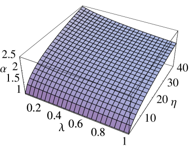
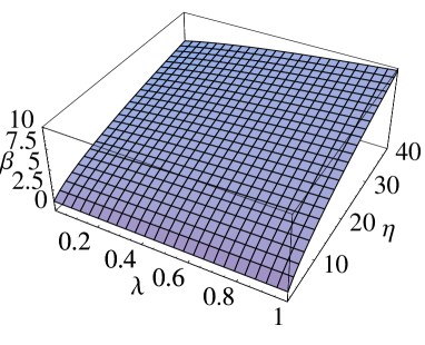
Figure 6: The functions $\alpha$ (left) and $\beta$ (right) vs. $\lambda$ and $\mu$.[color online.]

The functions $\alpha(\eta)$ and $\beta(\eta)$ (see Fig. 6) are increasing functions of $\eta$, and will provide us with a second expansion parameter. Now we separate variable in $x$ and $\eta$ as before,

$$\phi(\xi,\eta)=f(x)g(\eta)\quad,$$

which leads us to the following generalization of (29)

$$-\eta g^{\prime\prime}(\eta)f(x)+\beta(\eta)g(\eta)\left(-f^{\prime\prime}(x)+V_{\tilde{\lambda}(\eta)}(x)f(x)\right)-\\ \frac{\beta(\eta)^{2}\alpha^{\prime}(\eta)^{2}}{4\eta}g(\eta)\left(3xf^{\prime}(x)+x^{2}f^{\prime\prime}(x)\right)\\ -\beta(\eta)\alpha^{\prime}(\eta)xf^{\prime}(x)g^{\prime}(\eta)+\frac{1}{2}\beta(\eta)\alpha^{\prime\prime}(\eta)xf^{\prime}(x)g(\eta)=Ef(x)g(\eta)\quad.$$ (38)

We now ignore all but the first three terms– it can be verified numerically that all other terms are small–and separate variables

$$-f^{\prime\prime}(x)+V_{\tilde{\lambda}}f(x) = \epsilon(\tilde{\lambda}(\eta))f(x)\quad,$$ (39)

$$-\eta g^{\prime\prime}(\eta)+\beta(\eta)\epsilon(\tilde{\lambda}(\eta))g(\eta) = 0\quad.$$ (40)

The value $\beta(\eta)$ is larger than $\eta^{1/2}$, its value when $\lambda=0$, as can be seen in Fig.  6. The eigenvalue $\epsilon(\tilde{\lambda})$ is larger than $\sqrt{2}$, if we take $\eta$ large enough so that $\tilde{\lambda}={\cal O}(1)$, see Fig. 7. Since $\tilde{\lambda}\rightarrow 0$ for $\eta\rightarrow\infty$, we then have a rapid decay of the wave function for large $\eta$, as expected.

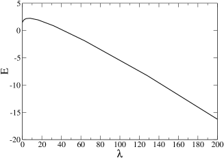
Figure 7: The lowest eigenvalue of the 1D Schrödinger equation (39) as a function of $\lambda$.

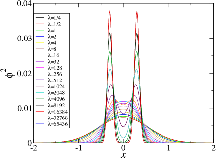
Figure 8: The lowest eigenfunction of (39) as a function of $\lambda$. [color online.]

The equation for $f(x)$ is interesting for other reasons as well; as shown in figure 8, we find that for large values of $\lambda$ the wave function separates into two parts. Remembering that $x=0$ corresponds to the lines $\rho_{1}=\pm\rho_{2}$, this supports our assertion that the wave function separates in 4 disjoint parts for large $\lambda$.

VI.2 Large values $\lambda>\lambda_{b}$

In the region of large coupling, the hyperbolic valleys of the free energy become very deep. We are interested in the asymptotics of the ground state wave function, when it becomes separated into four disjoint components. We continue to utilize the hyperbolic coordinates, but we shall now expand around the minima of the free energy.

In hyperbolic coordinates, the minimum of the free energy

$$\xi_{0}=\pm\frac{1}{2}\exp\left(-\frac{1+\lambda}{2\lambda}\right)$$

remains very close to $\xi=0$ (less than $\frac{1}{2\sqrt{e}}=0.303\ldots$ which is the value for $\lambda\rightarrow\infty$). Consequently the previous asymptotic analysis remains valid, and we can immediately conclude that the wave functions are decaying rapidly.

However, it is also of interest to consider the limit of a very deep potential directly, and for this we introduce coordinates from the minimum, scaled with $\xi_{0}$,

$$\xi=\xi_{0}(x\pm 1)\quad\&\quad\eta=\xi_{0}y\quad.$$

We then expand in powers of $x$, keeping leading terms only. The Hamiltonian simplifies to

$$H = -\frac{1}{\xi_{0}M}\sqrt{(1+x)^{2}+y^{2}}(\partial_{xx}+\partial_{yy})+2\lambda\xi_{0}^{2}(x+1)^{2}\left[\log(x+1)^{2}-1\right]$$ (41)

$$\approx -\frac{1}{\xi_{0}M}\sqrt{(1+y^{2}}(\partial_{xx}+\partial_{yy})+2\lambda\xi_{0}^{2}(-1+2x^{2})\quad.$$

With $\mu=\lambda\xi_{0}^{3}$ and $\epsilon=E\xi_{0}+\mu$ we this leads to the eigenvalue problem

$$-\frac{\sqrt{1+y^{2}}}{M}(\partial_{xx}\phi+\partial_{yy}\phi)+4\mu x^{2}\phi=\epsilon\phi\quad.$$ (42)

We now wish to consider the properties of solutions to this Schrödinger equation: We substitute

$$\phi(x,y)=f(z)g(y)\quad,$$

with

$$z=x(1+y^{2})^{1/8}\quad.$$

When we ignore terms containing lower order or mixed derivatives in addition of powers of $x$, we find that the equation takes the form

$$(1+y^{2})^{1/4}g(\frac{1}{M}\partial_{zz}f-4\mu z^{2}f)+f\sqrt{1+y^{2}}\frac{1}{M}\partial_{yy}g=\epsilon fg\quad.$$

Assuming again the lowest harmonic oscillator eigenstate for $f$,

$$f=\exp(-(z/b_{z})^{2}/2)\quad,$$

with

$$b_{z}=(2\mu M)^{-1/4}\quad,$$

we find for $g$,

$$-\frac{\sqrt{1+y^{2}}}{M}\partial_{yy}g+\sqrt{2\mu}(1+y^{2})^{1/4}g=\epsilon g\quad.$$

In order to obtain an analytic solution we shall assume $\mu$ to be so large that we again can make the harmonic approximation. This gives

$$-\partial_{yy}g+\sqrt{\mu/2}y^{2}g=(\epsilon-\sqrt{2\mu})g\quad.$$

Thus

$$g=\exp(-(y/b_{y})^{2}/2)\quad,$$

with $b_{y}=(8/M\mu)^{1/8}$, and the ground state energy is given by

$$\epsilon=(2\mu/M)^{1/2}+(\mu/(2M)^{3})^{1/4}\quad.$$

The energy for the original problem can thus be expressed as

$$E=\frac{(2\mu/M)^{1/2}+(\mu/(2M)^{3})^{1/4}-\mu}{\xi_{0}}\quad.$$

which is a good approximation only when the wave function $fg$ has no overlap with those from the remaining three valleys - and when our harmonic approximations are valid.

We also conclude that the scaling of the condensates observed in the previous section is indeed taking place; the width of both $f$ and $g$ depends on the combination $\mu M=\lambda M\xi_{0}^{3}$, and for large $\lambda$ $\xi_{0}$ is approximately constant, leading to the observed scaling in $\lambda M$. Since the wave function contract slowly to the maximum point (most slowly for $g$), we find that indeed we have in the limit $\lambda\rightarrow\infty$ the case where one of the two condensates disappears, as stated above. A further numerical analysis using the separated wave function confirms that this approach is very slow, and we must go to extremely high values of $\lambda$ to see the point where we can’t distinguish between the maximum and the expectation value of $\rho^{2}$.

VII Conclusions

In conclusion, we have investigated the phase structure of pure $SU(2)$ Yang-Mills theory using a slave-boson decomposition of the gauge field. We have employed a mean-field approximation where we account only for spatially homogeneous fluctuations in the gluonic holon fields. Our analysis suggests that the decomposed theory has an involved phase diagram, resembling that of cuprate superconductors. At intermediate couplings, there seems to be a gapped phase which is separated from the asymptotically free high energy limit by a pseudogap phase. Furthermore, we find that a mass gap appears to persists in the strong coupling limit even though asymptotically one of the two holon condensates appears to vanishes.

In our analysis we have employed a version of the maximal abelian gauge. In this gauge we have the advantage, that many results are available from first principle lattice simulations; see hay for a review. In particular, it has been observed hay that the (electric) confinement of color relates to the condensation of magnetic monopoles in the dual Higgs phase. Here we have inspected a (renormalization group invariant) perturbative one-loop approximation to the Yang-Mills effective action, in terms of decomposed variables that have a natural magnetic interpretation. Our results do not account for topologically nontrivial configurations, consequently it is not directly clear how our results could relate to the (electric) color confinement as observed in the lattice simulations. For a comparison, we need a first principles numerical lattice analysis in terms of the separated spin and charge variables. We also need a better understanding of electric-magnetic duality in terms of these variables. However, even at the level of the (crude) approximation that we employ here, it appears that when formulated in terms of the separate spin and charge variables the Yang-Mills theory has a very rich phase structure, not easily described in terms of the conventional gluonic variables. Our results suggests that the possibility of a spin-charge separation in the Yang-Mills theory may occur, and deserves to be addressed by extensive first-principles lattice simulations. Furthermore, there is a need to address theoretical issues such as electric-magnetic duality and the description of the Yang-Mills theory in terms of the spin-charge separated dual variables.

Indeed, if gluons can become decomposed into their independent holon and spinon components, it could have deep consequences to our understanding of the fundamental structure of matter.

- (1) P.W. Andersson, Science 235, 1196 (1987); L.D Faddeev and L.A. Takhtajan, Phys. Lett. A85, 375 (1981).
- (2) G. Baskaran, Z. Zhou and P.W. Andersson, Solid State Comm. 63, 973 (1987).
- (3) P.A. Lee, N. Nagaosa and X.-G. Wen, cond-mat/0410445.
- (4) L.D. Faddeev and A.J. Niemi, Phys. Lett. B525, 195 (2002).
- (5) A.J. Niemi, JHEP 0408, 035 (2004).
- (6) L.D. Faddeev and A.J. Niemi, Phys. Lett. B464, 90 (1999); B449, 214 (1999); Phys. Rev. Lett. 82 (1999) 1624
- (7) F.V. Gubarev, L. Stodolsky and V.I. Zakharov, Phys. Rev. Lett. 86, 2220 (2001); L Stodolsky, P. van Baal and V.I. Zakharov, Phys. Lett. B552, 214 (2003).
- (8) M.N. Chernodub and M.I. Polikarpov, in Confinement, duality, and nonperturbative aspects of QCD, P. van Baal, Ed. (Plenum Press, New York 1998); T. Suzuki, Prog. Theor. Phys. Suppl. 131, 633 (1998); R.W. Haymaker, Phys. Rept. 315, 153 (1999).
- (9) A.M. Polyakov, Phys. Lett. 59B, 122 (1978); M.E. Peskin, Ann. Phys. 113, 122 (1978).
- (10) L. Freyhult, Int.J.Mod.Phys. A17, 3681 (2002).
- (11) M. Lübke, A. J. Niemi, and K. Torokoff, Phys.Lett. B568, 176 (2003), hep-th/0301185.
- (12) P. H. Butler, Point Group Symmetry Applications (Plenum, New York, 1981).
- (13) B. Simon, Ann. Phys. (NY) 146, 209 (1983).
- (14) P. Moon and D.E. Spencer, Field theory handbook: including coordinate systems, differential equations and their solutions, 2nd Ed., (Springer-Verlag, Berlin, 1971).