Studying $W^{+}W^{-}$ production at the Fermilab Tevatron with SHERPA

Abstract

The merging procedure of tree-level matrix elements with the subsequent parton shower as implemented in SHERPA will be studied for the example of $W$ boson pair production at the Fermilab Tevatron. Comparisons with fixed order calculations at leading and next-to-leading order in the strong coupling constant and with other Monte Carlo simulations validate once more the impact and the quality of the merging algorithm and its implementation.

I Introduction

Studying the production of $W$ pairs at collider experiments offers a great possibility for tests of the gauge sector of the Standard Model, that has been extensively investigated by the LEP2 collaborations unknown:2003ih ; Barate:2000gi ; Abbiendi:2000eg ; Abdallah:2003zm ; Achard:2004zw . Tests in this channel are quite sensitive, because there is a destructive interference of two contributions: a $t$-channel contribution, where both $W$ bosons couple to incoming fermions, and an $s$-channel contribution, where the $W$ bosons emerge through a triple gauge coupling, either $\gamma W^{+}W^{-}$ or $ZW^{+}W^{-}$. New physics beyond the Standard Model could easily manifest itself, either through new particles propagating in the $s$-channel, like, for instance, a $Z^{\prime}$ particle in L-R symmetric models Pati:1974yy ; Mohapatra:1974hk ; Mohapatra:1980yp ; Eichten:1984eu , or through anomalous triple gauge couplings, which could be loop-induced, mediated by heavy virtual particles running in the loop. In Gaemers:1978hg ; Hagiwara:1986vm ; Bilenky:1993ms the most general form of an effective Lagrangian for such interactions has been developed and discussed. Such tests of anomalous triple gauge couplings have been performed both at LEP2 Abreu:1999vv ; Heister:2001qt ; Abbiendi:2003mk ; Achard:2004ji and at Tevatron, Run I Abe:1995jb ; Abachi:1997xe ; Abbott:1998gp ; Abbott:1998jz and at Run II Acosta:2005mu . Both scenarios could clearly modify the total cross section or, at least, lead to different distributions of the final state particles. In addition, $W$ pairs, possibly in association with jets, represent a background to a number of relevant other processes, such as the production of top quarks, the production of a Higgs boson with a mass above roughly 135 GeV, or the production of supersymmetric particles, such as charginos or neutralinos Abbott:1997rd ; Abe:1998qm .
Accordingly, there are a number of calculations and programs dealing with this process. At next-to-leading order (NLO) in the strong coupling constant, $W$ pair production has been calculated by Ohnemus:1991kk ; Frixione:1993yp ; Ohnemus:1994ff . In addition, a number of programs have been made available, allowing the user to implement phase space cuts and to generate single events. First of all, there are fixed order calculations. At leading order (LO), i.e. at tree-level, they are usually performed through automated tools, called matrix element or parton level generators. Examples for such programs include COMPHEP Pukhov:1999gg , GRACE/GR@PPA Ishikawa:1993qr ; GRAPPA , MADGRAPH/MADEVENT Stelzer:1994ta ; Maltoni:2002qb , ALPGEN Mangano:2002ea , and AMEGIC++ Krauss:2001iv . At NLO, the program MCFM Campbell:1999ah provides cross sections and distributions for this process.
Apart from such fixed order calculations, multipurpose event generators such as PYTHIA Sjostrand:2000wi ; Sjostrand:2001yu or HERWIG Corcella:2000bw ; Corcella:2002jc play a major role in the experimental analyses of collider experiments. They proved to be extremely successful in describing global features of such processes, like, for instance, the transverse momenta or rapidity distributions of the bosons. They are usually based on exact tree-level matrix elements for the production and decay of the boson pair, supplemented with a parton shower. The latter takes proper care of multiple parton emission and resums the corresponding leading and some of the subleading Sudakov logarithms.
In view of the need for increasing precision, recently two approaches have been developed that incorporate higher order corrections into the framework of multipurpose event generators. The first one, called MC@NLO, provides a method to consistently match NLO calculations for specific processes with the parton shower Frixione:2002ik ; Frixione:2003ei . The idea of this approach is to organize the counter-terms necessary to cancel real and virtual infrared divergencies in such a way that the first emission of the parton shower is recovered. Of course, this method depends to some extent on the details of the parton shower, and it has some residual dependence on the process in question. So far, MC@NLO has been implemented in conjunction with HERWIG Frixione:2004wy for the following processes: production of $W$ and $Z$ bosons, or pairs of these bosons Frixione:2002ik , production of the Higgs boson, production of heavy quarks Frixione:2003ei .
An alternative approach is to consistently combine tree-level matrix elements for different multiplicities of additional jets and to merge them with the parton shower. This approach has been presented for the first time for the case of $e^{+}e^{-}$ annihilations into jets Catani:2001cc ; later it has been extended to hadronic collisions Krauss:2002up and it has been reformulated to a merging procedure with a dipole shower in Lonnblad:2001iq . The idea underlying this method is to separate the kinematical range of parton emission by a $k_{\perp}$-algorithm Catani:1991hj ; Catani:1992zp ; Catani:1993hr into a regime of jet production, covered by the appropriate matrix elements, and a regime of jet evolution, covered by the respective shower. Then, the matrix elements are reweighted through Sudakov form factors and hard emissions in the parton shower leading to a jet are vetoed such that there is only a residual dependence on the jet resolution cut. This method is one of the cornerstones of the new event generator SHERPA Gleisberg:2003xi ; it has been validated for the cases of $e^{+}e^{-}$ annihilations into jets apacic2 ; Schaelicke:2005nv and for the production of single vector bosons at the Fermilab Tevatron Krauss:2004bs and the CERN LHC wz@LHC .
In this publication this series of studies will be continued with an investigation of $W$ pair production at the Fermilab Tevatron, Run II, where both $W$ bosons decay leptonically, i.e. $p\bar{p}\to W^{+}W^{-}+X\to e^{+}\mu^{-}\nu_{e}\bar{\nu}_{\mu}+X$. Input parameters used throughout this publication and the specifics, how the SHERPA runs have been obtained, are listed in the appendix, see Apps. A and C. After some consistency – including scale variation – checks of the merging algorithm in Sec. II, results obtained with SHERPA will be confronted with those from an NLO calculation provided by MCFM, cf. Sec. III. Then, in Sec. IV some exemplary results of SHERPA are compared with those obtained from other event generators, in particular with those from PYTHIA and MC@NLO. A summary closes this publication.

II Consistency checks

In this section some sanity checks of the merging algorithm for the case of $W$ pair production are presented. For this, first, the dependence of different observables on the key parameters of the merging procedure, namely the internal matrix-element parton-shower separation scale $Q_{\rm cut}$ and the highest multiplicity $n_{\rm max}$ of included tree-level matrix elements, is examined. Secondly, the sensitivity of the results with respect to changes in the renormalization scale $\mu_{R}$ and the factorization scale $\mu_{F}$ will be discussed.
All distributions shown in this section are inclusive results at the hadron level, where restrictive jet and lepton cuts have been applied, for details on the cuts cf. App. C. In all cases, the distributions are normalized to one using the respective total cross section as delivered by the merging algorithm.

Impact of the phase space separation cut

First of all, the impact of varying the jet resolution cut $Q_{\rm cut}$ is studied. SHERPA results have been obtained with an inclusive $2$jet production sample, i.e. tree-level matrix elements up to two additional QCD emissions have been combined and merged with the parton shower. In all figures presented here the black solid line shows the total inclusive result as obtained by SHERPA for the respective resolution cut $Q_{\rm cut}$. The reference curve drawn as a black dashed line has been obtained as the mean of five different runs, where the resolution cut has been gradually increased, $Q_{\rm cut}=10,15,30,50$ and $80$ GeV. The coloured curves represent the contributions stemming from the different matrix-element final-state multiplicities. Results are shown for three different resolution cuts, namely $Q_{\rm cut}=15,30$ and $80$ GeV. It should be noted that the change of the rate predicted by the merging procedure under $Q_{\rm cut}$ variation has been found to be very small, although it is a leading order prediction only. Nevertheless, by varying the separation cut between $10$ and $80$ GeV, the deviation of the total rate amounts to $2.4\%$ only.

Figure 1: The $p_{T}$ distribution of the $W^{+}$ boson and its dependence on $Q_{\rm cut}$, chosen to be $15$, $30$ and $80$ GeV (from top to bottom). The black solid line shows the SHERPA prediction obtained with $n_{\rm max}=2$, the black dashed one is the reference obtained as the mean of different $Q_{\rm cut}$ runs and the coloured lines indicate the different multiplicity contributions. The lower part of the plots exhibits the normalized difference of the prediction with respect to the reference. Cuts and input parameters are specified in the appendices.

Figure 2: The $p_{T}$ distribution of the $W^{+}W^{-}$ system under merging scale variation. The cut indicated through a vertical dashed-dotted line has been chosen as $Q_{\rm cut}=15$, $30$ and $80$ GeV (from top to bottom). The black solid line shows the SHERPA prediction obtained with $n_{\rm max}=2$, the black dashed one is the reference obtained as the mean of different $Q_{\rm cut}$ runs and the coloured lines indicate the different multiplicity contributions. The lower part of the plots exhibits the normalized difference of the prediction with respect to the reference. Cuts and input parameters are specified in the appendices.

Figure 3: Differential $1\to 0$ jet rate $Q_{1}$, $2\to 1$ jet rate $Q_{2}$ and $3\to 2$ jet rate $Q_{3}$ (left to right) for the SHERPA $n_{\rm max}=2$ configuration. The cut has been chosen to be $15$, $30$ and $80$ GeV (from top to bottom). The black solid line shows the total result, the black dashed one is the reference obtained as the mean of different $Q_{\rm cut}$ runs and the coloured lines indicate the different multiplicity contributions. The vertical dashed dotted line indicates the separation cut position. The lower part in all plots pictures the normalized difference of the corresponding prediction with respect to the reference. For input parameters and cuts, see Apps. A and C.

Figure 4: The $p_{T}$ distribution of the $W^{+}$ boson in dependence on the variation of the maximal jet number. The comparison is to a (black dashed) reference curve obtained with $n^{\rm ref}_{\rm max}=n_{\rm max}-1$. The cut has been chosen to be $15$ GeV. In both plots the black solid line shows the total result obtained with SHERPA. The coloured lines indicate the different multiplicity contributions. The lower part in both plots visualizes the normalized difference of the corresponding prediction with respect to the reference. For input parameters and cuts, see Apps. A and C.

As a first result, consider the $p_{T}$ distribution of the $W^{+}$ boson, presented in Fig. 1. The distributions become slightly softer for increasing cuts. However, this observable is very stable under variation of $Q_{\rm cut}$ with maximal deviations on the $\pm 5\%$ level only. The shape of the $W^{+}$ boson’s $p_{T}$ is already described at LO (using a parton shower only). As it can be seen from the figure, this LO dominance is nicely kept by the SHERPA approach under $Q_{\rm cut}$ variation. There the $1$jet (green line) and $2$jet (blue line) contributions are reasonably – for the $80$ GeV run, even strongly – suppressed with respect to the leading contribution.
In Fig. 2 the transverse momentum spectrum of the $W^{+}W^{-}$ system is depicted. Here, deviations show up, but they do not amount to more than $\pm 20\%$. Thus, the QCD radiation pattern depends only mildly on $Q_{\rm cut}$ (indicated by a vertical dashed-dotted line), which at the same time has been varied by nearly one order of magnitude. For $Q_{\rm cut}=15$ GeV the matrix element domain is enhanced with respect to the reference resulting in a harder $p_{T}$ tail. In contrast by using $Q_{\rm cut}=80$ GeV the hard tail of the diboson transverse momentum is underestimated with respect to the reference, since the parton shower attached only to the lowest order matrix element starts to fail in the description of high-$p_{T}$ QCD radiation at $p_{T}\approx 30$ GeV. At $Q_{\rm cut}=80$ GeV a smooth transition is required. The higher order matrix elements then stop the decrease in the $p_{T}$ prediction.
In previous publications it turned out that differential jet rates most accurately probe the merging algorithm, since they most suitably reflect the interplay of the matrix elements and the parton shower in describing QCD radiation below and above the jet resolution cut. Results obtained with the Run II $k_{\perp}$-algorithm using $R=1$ are shown for the $1\to 0$, $2\to 1$ and $3\to 2$ transition in the left, middle and right panels of Fig. 3, respectively. The value for the internal cut increases from $Q_{\rm cut}=15$ GeV (top) to $Q_{\rm cut}=80$ GeV (bottom). Compared with the $p^{WW}_{T}$ spectra, similar characteristics of deviations from the reference curve appear. However, here, they are moderately larger reaching up to $\pm 30\%$. The dashed dotted vertical line again marks the position of $Q_{\rm cut}$, which also pictures the separation of the $n$jet from the $n+1$jet contribution. Small holes visible around the respective separation cuts are due to a mismatch of matrix element and parton shower kinematics. For $Q_{\rm cut}=80$ GeV these holes are much more pronounced, reflecting the failure of the parton shower in filling the hard $p_{T}$ emission phase space appropriately.
Taken together, the deviations found are very moderate; however, in certain phase space regions they may reach up to $30\%$. This is satisfactory, since the merging algorithm guarantees $Q_{\rm cut}$ independence on the leading logarithmic accuracy only. The residual dependence of the results on $Q_{\rm cut}$ may be exploited to tune the perturbative part of the Monte Carlo event generator.

Impact of the maximal number of included matrix elements

Figure 5: The $H_{T}$ distribution and its dependence on the variation of the maximal jet number. The separation cut has been chosen to be $15$ GeV. The green solid line shows the SHERPA prediction obtained with $n_{\rm max}=1$, the lighter dashed and the grey dotted one stand for the $n_{\rm max}=2$ and $n_{\rm max}=3$ prediction, respectively; the darkgreen dashed-dotted curve pictures the pure shower performance of SHERPA starting off with the lowest order matrix element. The lower part of the plot shows the normalized differences with respect to the $n_{\rm max}=1$ case. For input parameters and cuts, see Apps. A and C.

Figure 6: SHERPA predictions of the inclusive $p_{T}$ of the associated jets considered in dependence on the variation of the maximal jet number. The spectra of the hardest and the second hardest jet are depicted in the upper and the lower panel, respectively. The jet resolution cut has been taken to be $15$ GeV. The green solid line shows the result of the $n_{\rm max}=1$ sample, the brighter dashed and the grey dotted one stand for the $n_{\rm max}=2$ and $n_{\rm max}=3$ sample, respectively; the darkgreen dashed-dotted curve depicts the pure shower performance. The lower part of the plot shows the normalized differences with respect to the $n_{\rm max}=1$ case. For the jet definition, the Run II $k_{\perp}$-algorithm with $R=0.7$ and $p^{\rm jet}_{T}>15$ GeV has been used. For more details, see Apps. A and C.

The approach of varying the maximal jet number $n_{\rm max}$ can be exploited to further scrutinize the merging procedure. In all cases considered here, $Q_{\rm cut}$ has been fixed to $Q_{\rm cut}=15$ GeV. This maximizes the impact of higher order matrix elements. In spite of this, for very inclusive observables, the rates differ very mildly, the change is less than $2\%$.
In Fig. 4, once more the transverse momentum distribution of the $W^{+}$ gauge boson is presented, illustrating that the treatment of the highest multiplicity matrix elements (for more details cf. Krauss:2004bs ; Schaelicke:2005nv ) completely compensates for the missing $2$jet matrix element in the $n_{\rm max}=1$ case. The behaviour is almost unaltered when changing from the $n_{\rm max}=1$ to the $n_{\rm max}=2$ prediction (cf. the right panel). In contrast, $n_{\rm max}=0$ yields a considerably softer distribution (cf. the left panel).
Lepton $p_{T}$ spectra show similar characteristics like the $W^{+}$ distribution. However, there are a number of observables, which turned out to be rather stable under the variation of $n_{\rm max}$, such as the pseudo-rapidity spectra of the $W^{+}$ boson, the positron and muon or correlations between the leptons, e.g. the $\Delta\phi$ or $\Delta R$ distribution. In these cases, deviations turn out to be smaller than $\pm 5\%$ in total, i.e. when considering the change between the pure shower and the inclusive $3$jet production performance of SHERPA. Even the pseudo-rapidity spectra of the resolved jets are rather unaffected.
In contrast, three more observables are presented showing a sizeable ($<\pm 30\%$) or even strong ($\approx\pm 100\%$) dependence on the variation of the maximal jet number, namely the $H_{T}$ distribution depicted in Fig. 5 and the inclusive $p_{T}$ spectra of associated jets exhibited in Fig. 6. The upper and lower panel of Fig. 6 shows the spectra of the hardest and the second hardest jet, respectively. Owing to the nature of these three observables to be sensitive on extra jet emissions, predictions – as expected – become harder with the increase of $n_{\rm max}$. However, a stabilization of the predictions is clearly found with the inclusion of more higher order matrix elements describing real QCD emissions.

Effects of renormalization and factorization scale variations

Figure 7: The $p_{T}$ distribution of the $W^{+}$ boson under scale variations. All predictions stem from SHERPA with $n_{\rm max}=1$ and $Q_{\rm cut}=15$ GeV. The green solid line shows the prediction under default scale choices for the merging procedure. For the black dashed and the black dotted curve, all scales for the coupling constants and PDFs have been multiplied by $0.5$ and $2.0$, respectively. The lower part of the plot presents the normalized differences with respect to the default choice. Input parameters and cuts are given in Apps. A and C.

Figure 8: The $H_{T}$ distribution and its dependence on the variation of $\mu_{R}$ and $\mu_{F}$ in the merging prescription. Fixing $n_{\rm max}=1$ and $Q_{\rm cut}=15$ GeV, the green solid line shows the prediction under default scale choices. For the black dashed and the black dotted curve, all scales for the coupling constants and PDFs have been multiplied by $0.5$ and $2.0$, respectively. The lower part of the plot presents the normalized differences with respect to the default choice. Input parameters and analysis cuts are given in Apps. A and C.

Figure 9: The $p_{T}$ distribution of the $W$ pair under variation of $\mu_{R}$ and $\mu_{F}$. Fixing $n_{\rm max}=1$ and $Q_{\rm cut}=15$ GeV, the green solid line shows the prediction under default scale choices. The black dashed and the black dotted curve is generated when all scales used for the coupling constants and PDFs have been multiplied by $0.5$ and $2.0$, respectively. The lower part of the plot presents the normalized differences with respect to the default choice. Input parameters (including a primordial $k_{\perp}$ smearing) and cuts are given in Apps. A and C.

In the following the impact of renormalization and factorization scale variations is discussed. For the SHERPA merging approach, this variation (also cf. wz@LHC ) is performed by multiplying all scales with a constant factor in all coupling constants and PDFs, which are relevant for the matrix element evaluation, the Sudakov weights and for the parton shower evolution.
For this study, the SHERPA samples are produced with $n_{\rm max}=1$ and $Q_{\rm cut}=15$ GeV. In all figures the green solid line represents SHERPA’s default scale choices, whereas the black dashed and the black dotted curve show the outcome for scale multiplications by $0.5$ and $2.0$, respectively. The total rate as provided by the merging algorithm is again remarkably stable, varying with respect to the default only by $\pm 4.2\%$, thereby increasing for smaller scales.
The transverse momentum distribution of the $W^{+}$ boson is investigated in Fig. 7. Scale variations slightly distort the shape, shifting it towards harder $p_{T}$ for smaller scales and vice versa. The effect is more pronounced in the $H_{T}$ distribution, shown in Fig. 8, and in the transverse momentum distribution of the diboson system, depicted in Fig. 9. However, the deviations maximally found reach up to $\pm 30\%$. In contrast to the findings stated so far, jet transverse momentum spectra do not feature shape distortions under scale variations.
The pattern found from these investigations can be explained as follows. The single matrix element contributions – here the $0$jet and $1$jet contribution – have their own rate and shape dependencies under scale variations. In their interplay these differences transfer to changing the admixture of the single contributions. Hence, shape modifications can appear as soon as different phase space regions are dominated by a single contribution. This also explains the behaviour found for jet $p_{T}$s. In the case studied here, they are solely described by the $1$jet matrix element with the parton shower attached, thus, their different rates cancel out due to normalization and their shapes are not affected.
Taken together, the dependencies found here, together with the ones on $Q_{\rm cut}$ and $n_{\rm max}$, yield an estimate for the uncertainty related to the SHERPA predictions.

III SHERPA comparison with MCFM

In this section, the focus shifts from internal sanity checks to comparisons with a full NLO calculation. For this, the MCFM program Campbell:1999ah has been used. In both, MCFM and SHERPA  the CKM matrix has been taken diagonal, and no $b$ quarks are considered in the partonic initial state of the hard process. If not stated otherwise, in MCFM the renormalization and factorization scale have been chosen as $\mu_{R}=\mu_{F}=M_{W}$, according to the choice made in Campbell:1999ah . For more details on the input parameters and setups, see Apps. A and B. In the following the results of MCFM are confronted with those of SHERPA (using $Q_{\rm cut}=15$ GeV) obtained at the parton shower level. Furthermore, for this analysis, realistic experimental cuts (cf. App. C) have been applied and all distributions have been normalized to one.
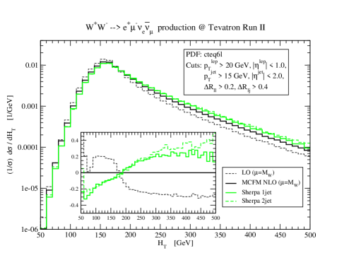
First the $H_{T}$ distribution, depicted in Fig. 10, is considered. Clearly, higher order corrections affect the $H_{T}$ shape. This is due to two reasons. First of all, the additional QCD radiation may manifest itself as jet(s), which thus contribute to $H_{T}$. Otherwise the additional partons still form a system against which the $W$ pair may recoil. Quantitatively, the inclusion of NLO results in a shift of the $H_{T}$ distribution at harder values by up to $20\%$; in SHERPA this trend is amplified by roughly the same amount. The differences between MCFM and SHERPA, however, are due to the different scale choices in both codes. In MCFM all scales have been fixed to $\mu=M_{W}$, whereas, forced by the merging procedure, in SHERPA the scales are set dynamically. In view of the scale variation results discussed in the previous section for $H_{T}$ (cf. Fig. 8) deviations of this magnitude owing to different scale choices are possible.

Figure 10: Normalized $H_{T}$ distribution. SHERPA results are shown for $n_{\rm max}=1$ (green solid line) and $n_{\rm max}=2$ (green dashed line) and compared to the QCD NLO result of MCFM (black solid line). The LO result with the same scale choice is depicted as a thin black dashed line. A difference plot with the MCFM NLO prediction as reference is given within the figure.

Figure 11: Normalized $H_{T}$ distribution. Here both, the renormalization and factorization scale of the NLO calculation have been varied in the range $\mu_{R}=\mu_{F}=M_{W}\ldots 4\,M_{W}$, indicated by the shaded area. These MCFM results are compared with the leading order result at $\mu_{R}=\mu_{F}=2\,M_{W}$ (thin black dashed line) and with the result of SHERPA where $n_{\rm max}=1$ (green solid line). The lower part of the plot shows the normalized differences with respect to the SHERPA result.

Figure 12: Normalized $H_{T}$ distribution in exclusive $p\bar{p}\to e^{+}\mu^{-}\nu_{e}\bar{\nu}_{\mu}$ production. The SHERPA result (green solid line) is obtained with $n_{\rm max}=0$ and a parton shower constrained not to produce any extra jets. This result is compared with the MCFM result at NLO in $\alpha_{s}$ (black solid line) and with the LO result (thin black dashed line). The latter two are taken for the default scale choices. The lower part of the plot shows the normalized differences with respect to the NLO result obtained from MCFM.

Figure 13: Normalized $p_{T}$ distribution of the $W$ pair. The MCFM result at $\mu_{R}=\mu_{F}=M_{W}$ (black line) is contrasted with the predictions made by SHERPA  both at the matrix element level (blue line) and at the parton shower level with $n_{\rm max}=0$ (darkgreen dotted line) and $n_{\rm max}=1$ (green solid line). A primordial $k_{\perp}$ smearing has been used to obtain the SHERPA shower results.

Figure 14: Normalized $\Delta\Phi^{\star}_{WW}$ distribution of the $W$ boson system. The MCFM result (black line) is contrasted with results from SHERPA at the parton shower level with $n_{\rm max}=0$ (darkgreen dotted line), $n_{\rm max}=1$ (green solid line) and $n_{\rm max}=2$ (green dashed line). Again a primordial $k_{\perp}$ smearing has been used. Additionally, the blue dashed curve represents a prediction obtained with MC@NLO. The lower part of the plot shows the normalized differences with respect to the result of MCFM.

Figure 15: Normalized transverse momentum distribution of the $W^{+}$ boson. The results of SHERPA for $n_{\rm max}=1$ (green solid line) and for $n_{\rm max}=2$ (green dashed line) are compared with the QCD NLO result obtained by MCFM (black solid line) and with the LO result (thin black dashed line) for the default scale choices, i.e. $\mu_{R}=\mu_{F}=M_{W}$. Within the plot the normalized differences with respect to the NLO result of MCFM are given.

Figure 16: Normalized transverse momentum distribution of the $e^{+}$ produced in the decay of the $W^{+}$. The results of SHERPA for $n_{\rm max}=1$ (green solid line) and for $n_{\rm max}=2$ (green dashed line) are confronted with the QCD NLO result obtained by MCFM (black solid line) and with the LO result (thin black dashed line). For the latter two, the scales are again fixed according to the default choices, i.e. $\mu_{R}=\mu_{F}=M_{W}$. Within the plot the normalized differences with respect to the NLO result of MCFM are shown.

Figure 17: Normalized $\eta$ distribution of the $W^{+}$ boson. The SHERPA results for $n_{\rm max}=1$ (green solid line) and $n_{\rm max}=2$ (green dashed line) are confronted with those of MCFM (black solid line) and with the LO result (thin black dashed line). Again, in the latter two the scales are chosen as $\mu_{R}=\mu_{F}=M_{W}$. The normalized differences with respect to the NLO result of MCFM are also shown.

Figure 18: Normalized $\Delta R$ distribution between the two charged leptons, the positron and the muon, emerging from the $W$ decays. SHERPA results for $n_{\rm max}=1$ (green solid line) and $n_{\rm max}=2$ (green dashed line) are compared to those predicted by MCFM (black solid line). The LO result with the same scale choice, is shown as a black dashed line. The lower part of the plot shows the normalized differences with respect to the NLO result of MCFM.

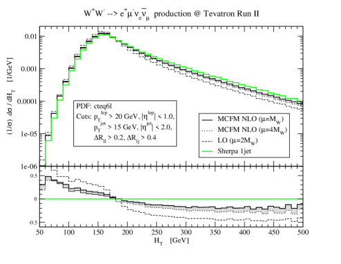
The impact of scale variations on the shape of the same observable is quantified in Fig. 11. This time, however, the SHERPA result with $n_{\rm max}=1$ is compared to NLO results obtained from MCFM with scale choices in the range $\mu_{R}=\mu_{F}=M_{W}\ldots 4\,M_{W}$ and with a LO result taken at $\mu_{R}=\mu_{F}=2M_{W}$. Obviously, the smaller choice of scale results in the MCFM outcome to be closer to the one of SHERPA. As expected, in comparison to the scale variation results found for SHERPA, the shape uncertainties of the full NLO prediction due to varying the scales are smaller.
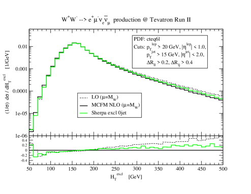
In Fig. 12, $H_{T}$ is depicted again, this time for the case of exclusive $p\bar{p}\to e^{+}\mu^{-}\nu_{e}\bar{\nu}_{\mu}$ production. There, the real part of the NLO correction in MCFM is constrained such that it does not produce an extra jet (for jet definition, see App. C). In SHERPA the $0$jet matrix element with the parton shower attached is considered exclusively, i.e. the parton shower is now forced not to produce any jet at all. In this case, the higher order corrections lead to a softer $H_{T}$ distribution compared to the leading order prediction, and the results of MCFM and SHERPA show the same deviations as before (cf. Fig. 10).
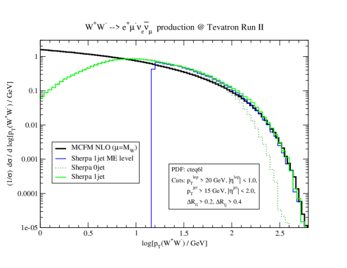
The effect of QCD radiation is best observed in the $p_{T}$ distribution of the $W$ pair, depicted in Fig. 13. Clearly, without any radiation, the $p_{T}$ of the $W$ pair is exactly zero, and only the emission of partons leads to a recoil of the diboson system. In the NLO calculation of MCFM, however, the spectrum is therefore described at lowest order, in this particular case taken at $\mu_{R}=\mu_{F}=M_{W}$. In contrast, in the SHERPA matrix element result, subjected to the explicit jet cut, Sudakov form factors and $\alpha_{s}$ reweighting are applied with a variable scale choice, explaining the differences between the two matrix-element type results in this figure. Contrasting this with the parton shower approach, it is clear that parton emission through the shower alone is not sufficient to generate sizeable $p_{T}$ of the $W$ pair in the hard region. For this, the corresponding matrix element has to be employed, leading to a very good agreement with the MCFM outcome in the high-$p_{T}$ tail of the distribution. In the soft regime the result of the bare MCFM matrix element is unphysical. Due to the cascade emission of soft and collinear partons, SHERPA accounts for resummation effects, which clearly yield the depopulation of the softest-$p_{T}$ region.
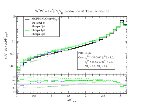
Another way to look at the effects of QCD radiation is to consider the relative angle between the two $W$ bosons, see Fig. 14. Of course, when they decay into leptons plus neutrinos this is not an experimental observable, on the generator level, however, it is very nice to visualize the effect of QCD radiation in this way. Without any QCD radiation, the two $W$s would be oriented back-to-back, at $\Delta\Phi^{\star}_{WW}=\pi$. Including QCD radiation, this washes out, as depicted in the figure. Again, resummation effects alter the result of the matrix element alone by decreasing the amount of softest radiation, this time corresponding to the back-to-back region around $\Delta\Phi^{\star}\approx\pi$. The effect of high-$p_{T}$ radiation can be clearly seen for small $\Delta\Phi^{\star}$ by comparing the different $n_{\rm max}$ predictions of SHERPA. The larger $n_{\rm max}$ is chosen, the harder the prediction for small $\Delta\Phi^{\star}$. On the other hand to better value the influence of the parton shower a prediction made by MC@NLO (see App. B) has been included. For a wide region of $\Delta\Phi^{\star}$, it well agrees with the SHERPA result for $n_{\rm max}=1$.
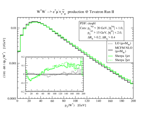
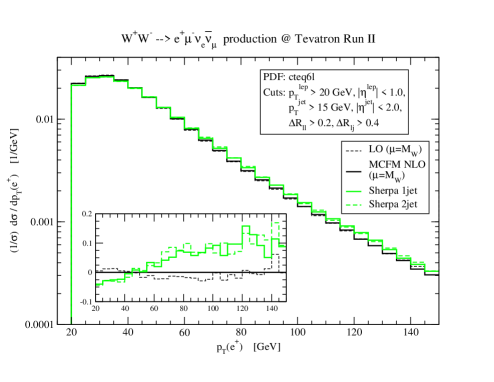
Figs. 15 and 16 exhibit the transverse momentum distributions of the $W^{+}$ and of the $e^{+}$ produced in its decay, respectively. Only mild deviations less than $10\%$ between MCFM and SHERPA are found, which again can be traced back to different scale choices in both approaches. These differences recur as and, therefore, explain part of the deviations found in the $H_{T}$ spectrum, cf. Fig. 10. As expected, the inclusion of the $2$jet contribution in SHERPA gives no further alterations of the $n_{\rm max}=1$ result. 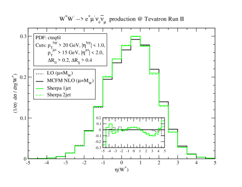Of course, the different radiation patterns also have some minor effects on the $\eta$ distribution of the $W^{+}$ depicted in Fig. 17. 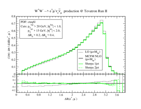In the $\Delta R_{e\mu}$ distribution presented in Fig. 18, the NLO result of MCFM and the parton shower level results of SHERPA are in nearly perfect agreement with each other. Higher order effects tend to change the shape of the LO prediction with respect to the NLO one by roughly $10\%$. The interesting observation here is that this change is seemingly not related to the transverse hardness of a jet system against which the $W$ pair recoils. This gives rise to the assumption that the change with respect to the LO result is due to some altered spin structure in the $2\to 5$ matrix element.

IV Comparison with other event generators

In this section a comparison of SHERPA with other hadron level event generators, in particular PYTHIA and MC@NLO will be discussed. Details on how their respective samples have been produced can be found in the Apps. A and B. The SHERPA samples have been generated with $n_{\rm max}=1$ and $Q_{\rm cut}=15$ GeV. The comparison is again on inclusive distributions – normalized to one – under the influence of realistic experimental cuts, for details see App. C.

Comparison of the QCD activity

Figure 19: Normalized $H_{T}$ distribution obtained from PYTHIA (red dotted line), MC@NLO (blue dashed line) and SHERPA (green solid line). For the generation of the SHERPA sample, $n_{\rm max}=1$ and $Q_{\rm cut}=15$ GeV have been chosen. The lower part of the plot exhibits the normalized differences with respect to the SHERPA prediction. Input parameters and the employed cuts are specified in the Apps. A and C.

Figure 20: Normalized $p_{T}$ distribution of the $W^{+}W^{-}$ system. Results from PYTHIA (red dotted line), MC@NLO (blue dashed line) and SHERPA (green solid line) are compared. For the generation of the latter, $n_{\rm max}=1$ and $Q_{\rm cut}=15$ GeV have been chosen. The lower part of the plot presents the normalized differences with respect to the SHERPA prediction. Input parameters (including a primordial $k_{\perp}$ smearing) and the employed cuts are specified in the Apps. A and C.

Figure 21: Difference of the scalar transverse momenta of the two $W$ bosons, $|p^{W^{+}}_{T}-p^{W^{-}}_{T}|$. The predictions compared are: PYTHIA given as a red dotted curve, MC@NLO depicted by the blue dashed line and SHERPA in inclusive $1$jet production at $Q_{\rm cut}=15$ GeV drawn as a green solid line as well as SHERPA in pure shower performance shown as a darkgreen solid line. The lower part of the plot shows the normalized differences with respect to the SHERPA prediction with $n_{\rm max}=1$. Input parameters and the employed cuts are summarized in the Apps. A and C.

Figure 22: Transverse momentum distributions of the associated jets, in the upper panel, the inclusive $p_{T}$ of the hardest jet is depicted, whereas in the lower panel that one of the second hardest jet is displayed. Again, results from PYTHIA are given by the red dotted lines, MC@NLO results are represented as blue dashed lines and SHERPA results are the green solid lines. For the generation of the latter, $n_{\rm max}=1$ and $Q_{\rm cut}=15$ GeV have been used. The lightgreen solid line in the lower panel corresponds to the SHERPA result obtained with $n_{\rm max}=2$. The lower part of both plots shows the normalized differences with respect to the SHERPA $n_{\rm max}=1$ performance. The input parameters and the employed cuts are summarized in the Apps. A and C.

As before, the starting point is the discussion of the radiation activity predicted by the various codes. In Fig. 19, results for the $H_{T}$ observable obtained from PYTHIA, MC@NLO and SHERPA are displayed. The predictions of the former two codes nicely agree with each other. Similar to the SHERPA MCFM comparison, SHERPA again predicts a slightly harder spectrum, with relative deviations of up to $20\%$.
Closer inspection of the reason for the differences in the $H_{T}$ spectrum reveals that the agreement of PYTHIA and MC@NLO is presumably a little bit accidental. A first hint into that direction can be read off Fig. 20, where the $p_{T}$ spectrum of the $W$ pair is displayed. In the region of low $p_{T}$ (up to $100$ GeV), the results of MC@NLO and SHERPA are in fairly good agreement, and sizeable differences larger than $10\%$ appear only for $p_{T}>100$ GeV. In contrast, the PYTHIA result for this observable shows a significant enhancement of the low-$p_{T}$ region and stays well below the other predictions for $p_{T}>10$ GeV. This comparison of the three differential cross sections clearly underlines that the three codes differ in their description of the QCD emissions.
Fig. 21 depicts the norm of the scalar difference of the transverse momenta of the $W^{+}$ and $W^{-}$ gauge boson, $|p^{W^{+}}_{T}-p^{W^{-}}_{T}|$. This observable is sensitive to higher order effects, since at LO it merely has a delta peak at $p_{T}=0$ GeV. Again, the hardest prediction is delivered by SHERPA with $n_{\rm max}=1$, results from MC@NLO, PYTHIA, and the pure shower performance of SHERPA are increasingly softer. For $|\Delta p_{T}|>60$ GeV, this observable seems to depend more and more on the quality of modelling the hardest emission, which is intrinsically better described by MC@NLO and by SHERPA with $n_{\rm max}=1$. The fact that the PYTHIA shower performs better than the pure SHERPA shower for high $p_{T}$ differences can be traced back to the choice of starting scale for the shower evolution, which is either $s_{p\bar{p}}$ (PYTHIA) or $s_{WW}$ (SHERPA).
In fact, differences appear in the $p_{T}$ distributions of the hardest two jets, see Fig. 22. The upper part of this figure depicts the transverse momentum spectrum of the hardest jet. Surprisingly, although MC@NLO contains a matrix element for the emission of an extra jet, its $p_{T}$ distribution is considerably softer (by up to $40\%$) than the result of SHERPA generated with $n_{\rm max}=1$. This trend is greatly amplified when going to the spectrum of the second hardest jet. There, clear shape differences of the order of a factor $2$ between the SHERPA $1$jet sample and MC@NLO show up for $p_{T}\approx 180$ GeV. The surprise according to this figure is that PYTHIA and SHERPA using $n_{\rm max}=1$ almost agree on the $p_{T}$ distribution of the second jet, although they were different for the hardest jet. At that point it should be noted that the second jet in both cases, PYTHIA and SHERPA with $n_{\rm max}=1$, is produced by the parton shower only. Given the drastically larger shower start scale of PYTHIA, it seems plausible to achieve to some extent a compensation for the intrinsic parton shower deficiencies in filling the hard emission phase space. However, in the very moment, SHERPA events are generated with appropriate matrix elements, i.e. with $n_{\rm max}=2$, this distribution is dramatically different for the three codes with deviations larger than a factor $2$ for $p_{T}\approx 120$ GeV.
Taken together, these findings hint that the three codes differ in their modelling of the QCD activity, especially in those of the hardest QCD emission. For MC@NLO and SHERPA the latter can be traced back to the different ansatz in including the matrix element for this emission, where again different scale choices may trigger effects on the $20\%$ level.

Comparison of lepton observables

Finally, the leptons in the final state as described by the three event generators PYTHIA, MC@NLO and SHERPA will be investigated. There, some significant differences appear between SHERPA and PYTHIA on the one hand, and MC@NLO on the other hand. These differences are due to the fact that at the moment spin correlations of the $W$ decay products are not implemented in MC@NLO. To validate that effects are indeed due to the lack of spin correlations, SHERPA samples have been prepared, where these correlations are artificially switched off. Furthermore, in order to quantify these effects without any bias, results have been obtained without the application of any lepton and jet cuts.

Figure 23: Normalized $p_{T}$ spectrum of the positron. Results of PYTHIA (red dotted line) and SHERPA (green solid line) including spin correlations are confronted with those obtained from MC@NLO (blue dashed line) and with results from SHERPA, where spin correlations have been switched off (green dashed line). All predictions are generated without the use of cuts. The vertical dashed-dotted line is added to indicate the position of the usually employed lepton $p_{T}$ cut. For input parameters, see App. A. The lower part of the plot shows the normalized differences with respect to the SHERPA prediction including spin correlations.

Figure 24: Normalized $\eta$ spectrum of the positron. Results of PYTHIA (red dotted line) and SHERPA (green solid line) including spin correlations are compared with those obtained from MC@NLO (blue dashed line) and with results from SHERPA, where spin correlations have been switched off (green dashed line). All predictions are generated without any restriction. The vertical dashed-dotted lines are added to indicate the position of the usually employed lepton $\eta$ cuts. For input parameters, see App. A. The lower part of the plot shows the normalized differences with respect to the SHERPA prediction including spin correlations.

Figure 25: Normalized $\Delta\phi_{e\mu}$ distribution. Results of PYTHIA (red dotted line) and SHERPA (green solid line) including spin correlations are compared with those obtained from MC@NLO (blue dashed line) and with results from SHERPA, where spin correlations have been switched off (green dashed line). All predictions are obtained without the use of cuts. For input parameters, see App. A. The lower part of the plot shows the normalized differences with respect to the SHERPA prediction including spin correlations.

Figure 26: Normalized $\Delta R_{e\mu}$ distribution. Results of PYTHIA (red dotted line) and SHERPA (green solid line) including spin correlations are compared with those obtained from MC@NLO (blue dashed line) and with results from SHERPA, where spin correlations have been eliminated (green dashed line). All predictions are obtained without the use of cuts. For input parameters, see App. A. The lower part of the plot shows the normalized differences with respect to the SHERPA prediction including spin correlations.

Figure 27: In the left and middle panel the $p_{T}$ spectrum of the $W^{+}$ before and after the application of cuts is depicted, respectively. The right panel exhibits the $\eta$ distribution of the $W^{+}$ under the influence of these cuts. The predictions compared are: PYTHIA (red dotted line), SHERPA (green solid line), MC@NLO (blue dashed line) and SHERPA without correlations in the boson decays (green dashed line). For input parameters, see App. A. The lower part of the plots shows the normalized differences with respect to the SHERPA prediction including spin correlations.

The impact of the lack of spin correlations already becomes visible in one-particle observables, such as the $p_{T}$ or the $\eta$ spectrum of the positron produced in the $W^{+}$ decay. These are shown in Figs. 23 and 24, respectively. Confronting the two methods with each other, which correctly respect spin correlations, for the transverse momentum distribution of the $e^{+}$, the following pattern is revealed. Due to the consistent inclusion of higher order tree-level matrix elements, the SHERPA $n_{\rm max}=1$ setup produces a considerably harder spectrum than PYTHIA. In contrast, the distributions with no spin correlations both result in an even harder high-$p_{T}$ tail. They agree quite well up to $p_{T}=60$ GeV, hence, this coincidence may be assigned to the lack of spin correlations in the gauge boson decays. Above that region, the MC@NLO spectrum again becomes softer with respect to the SHERPA prediction where the spin correlations have been eliminated. The fact that all four predicted distributions alter in their shape is not solely triggered by the different spin correlation treatments, again, the different descriptions of QCD radiation clearly contribute to the deviations found.
In contrast, a simpler pattern is found for the aforementioned $\eta$ distribution of the $e^{+}$. The results of PYTHIA and SHERPA with spin correlations on the one hand and of MC@NLO and SHERPA without spin correlations on the other hand show perfect agreement. Differences between the two spin correlation treatments may, thereby, easily reach up to $40\%$.
The influence of spin correlations can also be seen in observables based on two particle correlations. As two illustrative examples take the $\Delta\phi$ and the $\Delta R$ distribution of the $e^{+}$ and the $\mu^{-}$ produced in the decay of the two $W$ bosons. Again, the corresponding spectra, which have been exhibited in Figs. 25 and 26, differ significantly in shape depending on whether spin correlations are taken into account or not.
The discussion of the impact of spin correlations is completed by exploring the influence of the application of experimental cuts (cf. App. C) on the shape of certain spectra. It is clear that superimposing specific jet and lepton cuts strongly affects the event sample. Here, the cuts are mainly on the $\eta$ and the $p_{T}$ of the leptons. In turn their distributions alter. The characteristics found for the cutfree case are not substantially changed by the applied cuts and by the renormalization of the spectra according to these given cuts indicated by the vertical lines in the Figs. 23 and 24. More interestingly, however, these distributions drive alterations to secondary observables. In the two-particle correlations mentioned before, the effects already present without applying cuts are enforced. The slopes of the $\Delta\phi$ distributions increase, amplifying the difference between both sets of predictions, the ones with and without spin correlations. The main change in the $\Delta R$ spectrum is an additional deviation between $0.2$ (the cut) and $2.0$, such that now the no-spin-correlation results are roughly $20\%$ above the other ones. The case is different for the pseudo-rapidity distribution of the $W^{+}$ boson. Without the application of cuts one starts off distributions that agree on the $10\%$ level. This is severely changed by the introduction of the cuts, see the rightmost panel of Fig. 27. In contrast to the aforementioned two-particle correlations, here the predictions without spin correlations are well separated from the other ones only after the application of the cuts. As a last example, consider the transverse momentum distribution of the $W^{+}$ boson. Both types of predictions stemming from uncutted (left panel) and from samples analysed with cuts (middle panel) are pictured in Fig. 27. The inclusion of cuts apparently brings MC@NLO and SHERPA including the full correlations into good agreement, but this clearly happened accidentally.
To summarize, the examples shown here, clearly hint that the superposition of spin correlations (or their absence) together with cuts triggers sizeable effects in both types of observables, such that have already shown deviations in the absence of cuts and, more crucially, such that have not. In specific cases, such as the $p_{T}$ spectrum of the $W^{+}$, this may possibly lead to misinterpretations of the results.

V Conclusion

In this work, the merging procedure for multiparticle tree-level matrix elements and the parton shower implemented in SHERPA has been further validated; this time, the case of $W$ pair production at the Fermilab Tevatron has been considered. First, it has been shown that the results obtained with SHERPA are widely independent of specific merging procedure details such as the choice of the merging scale and, for sufficiently inclusive observables, the number of extra jets covered by the tree-level matrix elements. In addition, it has been shown that the specific form of the spectra produced by SHERPA is nearly independent – with deviations less than $20\%$ – of the choice of the factorization scale and the renormalization scale.
Having established the self-consistency of the SHERPA results, they have been compared to those from an NLO calculation provided through MCFM. There, good agreement of the two codes has been found, again on the $20\%$ level. Thus it is fair to state that the SHERPA results for the shapes are within theoretical errors consistent with an NLO calculation. The inclusion of the parton shower connected with specific scale choices in SHERPA, however, produces a surplus of QCD radiation with respect to the single parton emission in the real part of the NLO correction in MCFM.
Finally, the results of SHERPA have been compared with those of other hadron-level event generators, namely with PYTHIA and MC@NLO. In this comparison it turned out that SHERPA predicts a significant increase of QCD radiation with respect to the other two codes. For the $p_{T}$ spectra of jets accompanying the two $W$ bosons, the differences are dramatic in the high-$p_{T}$ tails. In addition, the impact of spin correlations has been quantified. In the observables considered here, it reaches $20\ldots 50\%$. This may be even larger than the impact of higher order corrections.

Appendix A Input parameters of SHERPA

All SHERPA studies have been carried out with the cteq6l PDF set Pumplin:2002vw . The value of $\alpha_{s}$ has been chosen according to the corresponding value of the selected PDF, namely $\alpha_{s}=0.118$. The running of the strong coupling constant is determined by the corresponding two-loop equation, except for the SHERPA MCFM comparison. There an one-loop running has been employed for $\alpha_{s}$. Jets or initial partons are defined by gluons and all quarks but the top quark; this one is allowed to appear within the matrix elements only through the coupling of the $W$ boson with the $b$ quark. In the SHERPA MCFM comparison SHERPA runs, however are restricted to the light-flavour sector, i.e. the $g,\,d,\,u,\,s,\,c$ sector. In the matrix element calculation the quarks are taken massless, only the shower will attach current masses to them. The shower cut-offs applied are $2$ GeV and $1$ GeV for the initial and the final state emissions, respectively. If explicitly stated a primordial $k_{\perp}$ Gaussian smearing has been employed with both, mean and standard deviation being equal to $0.8$ GeV. The Standard Model input parameters are:

$$m_{W}=80.419\;{\rm GeV}\,,\quad\Gamma_{W}=2.06\;{\rm GeV,}$$

$$m_{Z}=91.188\;{\rm GeV}\,,\quad\Gamma_{Z}=2.49\;{\rm GeV,}$$

$$G_{\mu}=1.16639\times 10^{-5}\;{\rm GeV}^{-2},$$

$$\sin^{2}\theta_{W}=1-m^{2}_{W}/m^{2}_{Z},$$

$$\alpha_{s}=0.118.$$ (1)

The electromagnetic coupling is derived from the Fermi constant $G_{\mu}$ according to

$$\alpha_{\rm em}=\frac{\sqrt{2}\,G_{\mu}\,M^{2}_{W}\,\sin^{2}\theta_{W}}{\pi}\,.$$ (2)

The constant widths of the electroweak gauge bosons are introduced through the fixed-width scheme. The CKM matrix has been always taken diagonal.

Appendix B Setups for MCFM, MC@NLO and PYTHIA

MCFM
The program version employed is MCFM v4.0. The process chosen is nproc=61. The investigations have been restricted to the $d,\,u,\,s,\,c$ quark sector. The PDF set used is cteq6l. The default scheme for defining the electroweak couplings has been used and their input values have been adjusted with the corresponding parameter settings given for SHERPA. The renormalization scale and the factorization scale are fixed and set to $\mu_{R}=\mu_{F}=M_{W}$.

MC@NLO
The program version used is MC@NLO 2.31. The process number is taken as IPROC=-12850, so that the underlying event has not been taken into consideration. The two $W$ boson decays into leptons are steered by the two MODBOS variables being set to 2 and 3 for the first and the second choice, respectively. The lepton pairs have been generated in a mass window of

$$M_{W}-40\,\Gamma_{W}<m_{l\nu}<M_{W}+40\,\Gamma_{W}\,.$$ (3)

Again, the cteq6l PDF set as provided by MC@NLO’s own PDF library is used. The weak gauge boson masses and widths are aligned to the settings used for the previous codes. All other parameters have been left unchanged with respect to their defaults.

PYTHIA
The PYTHIA version used is 6.214. The process $p\bar{p}\to W^{+}W^{-}+X$ is selected through MSUB(25)=1. The specific decay modes of the two $W$’s are picked by putting MDME(206,1)=2 and MDME(207,1)=3, where all other available modes are set to zero. The possibility of parton shower emissions right up to the limit, which has been proven to be more convenient for jet production Miu:1998ju , is achieved with MSTP(68)=2. This increases the IS shower start scale in PYTHIA to $\sqrt{s}=1960$ GeV and accounts for a reasonably higher amount of hard QCD radiation. For all comparisons here, the underlying event is switched off, other parameters are left to their default.

Appendix C Phase space cuts

Two different analyses are used for the comparisons of the results obtained throughout this publication. A simple analysis has been taken to verify the pure behaviour of the considered programs. For this case, only jets are analysed utilizing the Run II $k_{\perp}$ clustering algorithm defined in Blazey:2000qt with a pseudo-cone size of $R=1$. The jet transverse momentum has to be greater than $15$ GeV.
For more realistic experimental scenarios, an analysis applying jet and lepton cuts has been availed. Then, the pseudo-cone size of the jet algorithm has been set to $R=0.7$, and the jets have to fulfil the following constraints on the pseudo-rapidity and the transverse momentum,

$$|\eta^{\rm jet}|<2.0\,,\quad p^{\rm jet}_{T}>15\ {\rm GeV}\,.$$ (4)

For the charged leptons the cuts on these observables are given by

$$|\eta^{\rm lep}|<1.0\,,\quad p^{\rm lep}_{T}>20\ {\rm GeV}\,,$$ (5)

however, a cut on the missing transverse energy has not been introduced. There is a final selection criteria corresponding to the separation of the leptons from each other and from the jets,

$$\Delta R_{\rm ll}>0.2\,,\quad\Delta R_{\rm lj}>0.4\quad\,.$$ (6)

References

- (1) [LEP Collaboration], arXiv:hep-ex/0312023.
- (2) R. Barate et al. [ALEPH Collaboration], Phys. Lett. B 484 (2000) 205 [arXiv:hep-ex/0005043].
- (3) G. Abbiendi et al. [OPAL Collaboration], Phys. Lett. B 493 (2000) 249 [arXiv:hep-ex/0009019].
- (4) J. Abdallah et al. [DELPHI Collaboration], Eur. Phys. J. C 34 (2004) 127 [arXiv:hep-ex/0403042].
- (5) P. Achard et al. [L3 Collaboration], Phys. Lett. B 600 (2004) 22 [arXiv:hep-ex/0409016].
- (6) J. C. Pati and A. Salam, Phys. Rev. D 10 (1974) 275.
- (7) R. N. Mohapatra and J. C. Pati, Phys. Rev. D 11 (1975) 566.
- (8) R. N. Mohapatra and G. Senjanovic, Phys. Rev. D 23 (1981) 165.
- (9) E. Eichten, I. Hinchliffe, K. D. Lane and C. Quigg, Rev. Mod. Phys. 56 (1984) 579 [Addendum-ibid. 58 (1986) 1065].
- (10) K. J. F. Gaemers and G. J. Gounaris, Z. Phys. C 1 (1979) 259.
- (11) K. Hagiwara, R. D. Peccei, D. Zeppenfeld and K. Hikasa, Nucl. Phys. B 282 (1987) 253.
- (12) M. S. Bilenky, J. L. Kneur, F. M. Renard and D. Schildknecht, Nucl. Phys. B 409 (1993) 22.
- (13) P. Abreu et al. [DELPHI Collaboration], Phys. Lett. B 459 (1999) 382.
- (14) A. Heister et al. [ALEPH Collaboration], Eur. Phys. J. C 21 (2001) 423 [arXiv:hep-ex/0104034].
- (15) G. Abbiendi et al. [OPAL Collaboration], Eur. Phys. J. C 33 (2004) 463 [arXiv:hep-ex/0308067].
- (16) P. Achard et al. [L3 Collaboration], Phys. Lett. B 586 (2004) 151 [arXiv:hep-ex/0402036].
- (17) F. Abe et al. [CDF Collaboration], Phys. Rev. Lett. 75 (1995) 1017 [arXiv:hep-ex/9503009].
- (18) S. Abachi et al. [D0 Collaboration], Phys. Rev. D 56 (1997) 6742 [arXiv:hep-ex/9704004].
- (19) B. Abbott et al. [D0 Collaboration], Phys. Rev. D 58 (1998) 031102 [arXiv:hep-ex/9803017].
- (20) B. Abbott et al. [D0 Collaboration], Phys. Rev. D 58 (1998) 051101 [arXiv:hep-ex/9803004].
- (21) D. Acosta et al. [CDF Collaboration], arXiv:hep-ex/0501050.
- (22) B. Abbott et al. [D0 Collaboration], Phys. Rev. Lett. 80 (1998) 442 [arXiv:hep-ex/9708005].
- (23) F. Abe et al. [CDF collaboration], Phys. Rev. Lett. 80 (1998) 5275 [arXiv:hep-ex/9803015].
- (24) J. Ohnemus, Phys. Rev. D 44 (1991) 1403.
- (25) S. Frixione, Nucl. Phys. B 410 (1993) 280.
- (26) J. Ohnemus, Phys. Rev. D 50 (1994) 1931 [arXiv:hep-ph/9403331].
- (27) A. Pukhov et al., arXiv:hep-ph/9908288.
- (28) T. Ishikawa, T. Kaneko, K. Kato, S. Kawabata, Y. Shimizu and H. Tanaka [MINAMI-TATEYA group Collaboration], KEK-92-19
- (29) K. Sato et al., Proc. VII International Workshop on Advanced Computing and Analysis Techniques in Physics Research (ACAT 2000), P. C. Bhat and M. Kasemann, AIP Conference Proceedings 583 (2001) 214.
- (30) T. Stelzer and W. F. Long, Comput. Phys. Commun. 81 (1994) 357 [arXiv:hep-ph/9401258];
- (31) F. Maltoni and T. Stelzer, JHEP 0302 (2003) 027 [arXiv:hep-ph/0208156].
- (32) M. L. Mangano, M. Moretti, F. Piccinini, R. Pittau and A. D. Polosa, JHEP 0307 (2003) 001 [arXiv:hep-ph/0206293].
- (33) F. Krauss, R. Kuhn and G. Soff, JHEP 0202, 044 (2002) [arXiv:hep-ph/0109036].
- (34) J. M. Campbell and R. K. Ellis, Phys. Rev. D 60 (1999) 113006 [arXiv:hep-ph/9905386].
- (35) T. Sjöstrand, P. Eden, C. Friberg, L. Lönnblad, G. Miu, S. Mrenna and E. Norrbin, Comput. Phys. Commun. 135 (2001) 238 [arXiv:hep-ph/0010017].
- (36) T. Sjöstrand, L. Lönnblad and S. Mrenna, arXiv:hep-ph/0108264.
- (37) G. Corcella et al., JHEP 0101 (2001) 010 [arXiv:hep-ph/0011363].
- (38) G. Corcella et al., arXiv:hep-ph/0210213.
- (39) S. Frixione and B. R. Webber, JHEP 0206 (2002) 029 [arXiv:hep-ph/0204244].
- (40) S. Frixione, P. Nason and B. R. Webber, JHEP 0308 (2003) 007 [arXiv:hep-ph/0305252].
- (41) S. Frixione and B. R. Webber, arXiv:hep-ph/0402116.
- (42) S. Catani, F. Krauss, R. Kuhn and B. R. Webber, JHEP 0111 (2001) 063 [arXiv:hep-ph/0109231].
- (43) F. Krauss, JHEP 0208 (2002) 015 [arXiv:hep-ph/0205283].
- (44) L. Lönnblad, JHEP 0205 (2002) 046 [arXiv:hep-ph/0112284].
- (45) S. Catani, Y. L. Dokshitzer, M. Olsson, G. Turnock and B. R. Webber, Phys. Lett. B 269 (1991) 432.
- (46) S. Catani, Y. L. Dokshitzer and B. R. Webber, Phys. Lett. B 285 (1992) 291.
- (47) S. Catani, Y. L. Dokshitzer, M. H. Seymour and B. R. Webber, Nucl. Phys. B 406 (1993) 187.
- (48) T. Gleisberg, S. Höche, F. Krauss, A. Schälicke, S. Schumann and J. Winter, JHEP 0402 (2004) 056 [arXiv:hep-ph/0311263].
- (49) F. Krauss, A. Schälicke and G. Soff, arXiv:hep-ph/0503087.
- (50) A. Schälicke and F. Krauss, arXiv:hep-ph/0503281.
- (51) F. Krauss, A. Schälicke, S. Schumann and G. Soff, Phys. Rev. D 70 (2004) 114009 [arXiv:hep-ph/0409106].
- (52) F. Krauss, A. Schälicke, S. Schumann and G. Soff, arXiv:hep-ph/0503280.
- (53) S. Frixione, private communication.
- (54) J. Pumplin, D. R. Stump, J. Huston, H. L. Lai, P. Nadolsky and W. K. Tung, JHEP 0207 (2002) 012 [arXiv:hep-ph/0201195].
- (55) G. Miu and T. Sjöstrand, Phys. Lett. B 449 (1999) 313 [arXiv:hep-ph/9812455].
- (56) G. C. Blazey et al., arXiv:hep-ex/0005012.