Electroweak properties of the $\pi$, $K$ and $K^{*}(892)$ in the three forms of relativistic kinematics

Abstract

The electromagnetic form factors, charge radii and decay constants of $\pi$, $K$ and $K^{*}(892)$ are calculated using the three forms of relativistic kinematics: instant form, point form and (light) front form. Simple representations of the mass operator together with single quark currents are employed with all the forms. Making use of previously fixed parameters, together with the constituent quark mass for the strange quark, a reasonable reproduction of the available data for form factors, charge radii and decay constants of $\pi$, $\rho$, $K$ and $K^{*}(892)$ is obtained in front form. With instant form a similar description, but with a systematic underestimation of the vector meson decay constants is obtained using two different sets of parameters, one for $\pi$ and $\rho$ and another one for $K$ and $K^{*}(892)$. Point form produces a poor description of the data.

1 Introduction

The understanding of electromagnetic and weak properties of low mass hadrons is still an open issue, mostly due to the fact that the theory of the strong interactions, QCD, cannot be easily solved at low energies. This includes, e.g., the description of the spectra of bound states of quarks, baryons and mesons, and reactions involving the excitation of resonances. These difficulties in solving QCD in the nonperturbative regime have triggered many investigations, more or less related to QCD, which try to shed some light on this domain.

One of these approaches, which we explored here, is the formulation of relativistic quark models with a fixed number of degrees of freedom. Relativistic quark models have been implemented in three ways, depending on the way in which the interactions are included in the commutator relations of the Poincaré algebra dirac ; keister . In principle the three ways should provide similar results. However, in practice, the use of simplifications, notably the use of single quark currents which permits a simpler picture of the process, forces the appearance of qualitative differences in the results.

In a previous work junhe the electromagnetic form factors of $\pi$ and $\rho$ were studied making use of three different forms of relativistic quantum mechanics. The ground state wave function was adjusted in each of the forms to describe both the charge radii and the high-$Q^{2}$ behavior of the pion charge form factor. It was found that front and instant forms permitted a reasonable reproduction of the pion form factors, and a coherent picture for the form factors and charge radii of $\rho$. With point form no ground state could be found, within the considered wave functions, such that the pion charge form factor would be qualitatively reproduced.

The main purpose of this work is to explore to what extent the mass operators which were fixed to reproduce $\pi$ form factors in each of the forms and which were applied to the study of its vector partner, $\rho$, are able to provide a description also of the other members of the $SU(3)_{f}$ octet, in our case the $K$ and the vector $K^{*}(892)$.

Comparison with experimental data for the case of the kaon form factor and decay constants and with some of the previous works done in any of the three forms of kinematics are given Chung:mu ; Cardarelli ; ChoiKaon ; Xiao ; Krutov ; Amghar:2003tx .

The point form used in this work, which follows Refs. Wagenbrunn ; Riska04 ; junhe , differs from the one discussed lately in Refs. Amghar:2003tx ; Desplanques02 where a closer contact with the original Dirac formulation is pursued. The formulation used here emphasizes the relevant fact that distinguishes among the forms which is the kinematic subgroup of the Poincaré group. Once a kinematic subgroup (“form of kinematics”) is chosen, the main difference between the forms of kinematics, when considering single quark currents, lies in the way the variables entering in the rest frame wave functions are related to the variables appearing in the interaction vertex. This distinction between the two formulations of the point form is not quantitatively very relevant for the case of two-body systems as was shown in Ref. Desplanques04 .

This article is organized in the following way: Section 2 presents the wave functions used. Then Section 3 contains the formulas needed to compute the form factors and decay constants of both spin-0 and spin-1 mesons, including mesons made up of quarks of different mass. The $\pi$ and the $K$ are studied in Section 4. The decay constants of $\rho$ and $K^{*}(892)$ and the form factors of the $K^{*}(892)$ are presented in Section 5. A summary and discussion are given in the last section.

2 Wave functions

In the rest frame, meson states are represented by eigenfunctions of the mass operator, which are functions of internal momenta, $\vec{k}_{i}$, and spin variables. A simple spectral representation of the mass operator, with meson wave functions constructed in the naive quark model Close , is considered,

$$\psi^{\pi(K)}({\vec{q}}) = \xi_{c}\,\varphi_{0}({\vec{q}})\,\phi_{S}\,\chi_{A}\,,$$

$$\psi^{\rho(K^{*})}({\vec{q}}) = \xi_{c}\,\varphi_{0}({\vec{q}})\,\phi_{A}\,\chi_{S}\,,$$ (1)

where $\xi_{c}$, $\phi_{S}$ and $\chi_{A}$ are the color, flavor and spin wave functions.

The effect of the Lorentz transformation on the spin variables for canonical spins is accounted by a Wigner rotation of the form:

$$D^{1/2}_{\lambda_{i},\sigma_{i}}\left(R_{W}[B(v_{K}),k_{i}]\right)$$ (2)

with

$$R_{W}[B(v_{K}),k_{i}]:=B^{-1}(p_{i})B(v_{K})B(k_{i})\,,$$ (3)

where $B(v)$ are rotationless Lorentz transformations, and $v_{K}$ is the boost velocity.

For the spatial part of the wave function, both Gaussian and rational forms are employed:

$$\varphi^{G}_{0}({\vec{q}}) = \frac{1}{(b\sqrt{\pi})^{3/2}}e^{-{\vec{q}}^{\,2}/2b^{2}}\,,$$

$$\varphi^{R}_{0}({\vec{q}}) = {\cal N}(1+{\vec{q}}^{\,2}/2b^{2})^{-a},$$ (4)

where ${\vec{q}}=\frac{1}{\sqrt{2}}({\vec{k}}_{2}-{\vec{k}}_{1})$ and ${\cal N}$ is a normalization constant. In the center of mass frame we have ${\vec{k}}_{1}+{\vec{k}}_{2}=0$ and thus $\vec{k}_{2}=\frac{1}{\sqrt{2}}\vec{q}=-\vec{k}_{1}$. As a starting point the parameters used in Ref. junhe which are given in Table 1 are employed.

	b [MeV]	$m_{q}$[MeV]	a	$m_{s}$[MeV]
Gaussian
Instant form	370 [470]	140 [200]	$--$	500
Point form	3000 [470]	380 [200]	$--$	500
Front form	450 [500]	250 [250]	$--$	400
Rational
Instant form	700 [520]	150 [250]	5 [3]	500
Point form	3000 [520]	300 [250]	1 [3]	500
Front form	600 [650]	250 [250]	3 [3]	400

Table 1: Parameters used in instant, point and front form both for the rational and gaussian spatial wave functions. In brackets are the readjusted sets of parameters as explained in the text in Section 4.

The Jacobian of the transformations between the variables are, for point form,

$$J(\vec{v};\vec{p}_{2}):=\left({\partial\vec{q}\over\partial\vec{p}_{2}}\right)_{\vec{v}}=2\sqrt{2}{(E_{2}v^{0}-p_{2z}v_{z})\over E_{2}}\,,$$ (5)

with

$$\omega_{i}=\sqrt{m_{i}^{2}+k_{i}^{2}}\,,\quad E_{i}=\sqrt{m_{i}^{2}+p_{i}^{2}}\,,$$ (6)

for front form

$$J({\bf P};{\bf p_{2}}) := \left({\partial\vec{q}\over\partial(\xi_{2},{\bf k}_{2\perp})}\right)_{\bf P}$$ (7)

$$= 2\sqrt{2}\frac{M_{0}}{4\xi(1-\xi)}\left[1-\left(\frac{m_{1}^{2}-m_{2}^{2}}{M_{0}^{2}}\right)^{2}\right]\,,$$

with

$$k_{zi} = {1\over 2}\left(\xi_{i}M_{0}-{m_{q}^{2}+k_{i\perp}^{2}\over\xi_{i}M_{0}}\right)\,,M_{0}^{2}=\sum_{i}{m_{i}^{2}+k_{i\perp}^{2}\over\xi_{i}},$$ (8)

and for instant form,

$${\cal}J(\vec{P},\vec{p}_{2}):=2\sqrt{2}\frac{\omega_{2}}{E_{2}}\left\{1-\frac{E_{2}v_{z}}{M_{0}}\left({p_{1z}\over E_{1}}-{p_{2z}\over E_{2}}\right)\right\},$$ (9)

where

$$P_{x}=P_{y}=0\;,\;M_{0}^{2}=(\sum_{i}E_{i})^{2}-|\vec{P}|^{2}\;,\;\vec{v}:={\vec{P}\over M_{0}}\,.$$ (10)

3 Meson electroweak properties

As in Refs. Chung:mu ; Riska04 the effective conserved electromagnetic current operator in each of the forms can be generated by the dynamics from a current which is covariant under the kinematic subgroup. Then, electromagnetic form factors of two-body systems can be defined as certain matrix elements of the electromagnetic current. In point and instant forms, the charge form factor of scalar mesons can be defined as follows,

$$F_{C}(Q^{2})=\langle 0,{\vec{Q}}/2|I^{0}(0)|0,-{\vec{Q}}/2\rangle_{c}$$ (11)

where $I^{0}$ is the time component of the current and ${\vec{Q}}$ has been taken to be parallel to the $z$-axis. The charge radii can be obtained by $\langle r^{2}\rangle_{\pi}=-6(dF_{C}/dQ^{2})_{Q^{2}=0}$·

In front form, in the $Q^{+}=0$ frame, the charge form factor is extracted from the “plus” component of the current, $I^{+}=n\cdot I$, with $n=\{-1,0,0,1\}$:

$$F_{C}(Q^{2})=\langle 0|I^{+}(0)|0\rangle\,,$$ (12)

in this case the momentum transfer is taken to be transverse to the $z$-direction Riska04 .

For vector mesons, such as the $\rho$ and the $K^{*}(892)$, the definition of Ref. Chung is adopted. For point and instant forms, we have:

$$G_{C}(Q^{2}) = {1\over 3}\left[\langle 0,{\textstyle{\vec{Q}\over 2}}|I^{0}(0)|-{\textstyle{\vec{Q}\over 2}},0\rangle_{c}\right.$$

$$\left.+2\langle 1,{\textstyle{\vec{Q}\over 2}}|I^{0}(0)|-{\textstyle{\vec{Q}\over 2}},1\rangle_{c}\right],$$

$$G_{M}(Q^{2}) = \sqrt{2\over\eta}\langle 1,{\textstyle{\vec{Q}\over 2}}|I_{+}(0)|-{\textstyle{\vec{Q}\over 2}},0\rangle_{c},$$ (13)

$$G_{D}(Q^{2}) = \frac{1}{2\eta}\left[\langle 0,{\textstyle{\vec{Q}\over 2}}|I^{0}(0)|-{\textstyle{\vec{Q}\over 2}},0\rangle_{c}\right.$$

$$\left.-\langle 1,{\textstyle{\vec{Q}\over 2}}|I^{0}(0)|-{\textstyle{\vec{Q}\over 2}},1\rangle_{c}\right],$$

where $I_{+}=(1/2)(I_{x}+iI_{y})$. For front form,

$$G_{C}(Q^{2})=F_{0d}+{\textstyle{1\over 6}}F_{2d}-{\textstyle{2\over 3}}\eta\left\{F_{0d}+F_{2d}+{\textstyle{5\over 2}}F_{1d}\right\},$$

$$G_{M}(Q^{2})=2F_{0d}+F_{2d}+F_{1d}(1-\eta),$$

$$G_{D}(Q^{2})=\frac{1}{\eta}\left\{F_{2d}+\eta\left({\textstyle{1\over 2}}F_{2d}-{F_{0d}-F_{1d}}\right)\right\}\,,$$ (14)

where

$$F_{0d}(Q^{2})=\frac{1}{2(1+\eta)}\{\langle 1|I^{+}(0)|1\rangle+\langle 0|I^{+}(0)|0\rangle\},$$

$$F_{1d}(Q^{2})=\frac{-\sqrt{2}}{\sqrt{\eta}(1+\eta)}\langle 1|I^{+}(0)|0\rangle,$$

$$F_{2d}(Q^{2})=\frac{-1}{(1+\eta)}\langle 1|I^{+}(0)|-1\rangle\,.$$ (15)

The kinematical variable $\eta$ is defined as $\eta={1\over 4}(v_{f}-v_{a})^{2}=Q^{2}/4M^{2}$, where $M$ is the meson mass.

For each form of kinematics the dynamics generates the current density operator from a kinematic current. For point form we have,

$$\langle{\vec{v}_{f},\vec{v}_{2}^{\prime}}|I^{\mu}(0)|{\vec{v}_{2},\vec{v}_{a}}\rangle=$$

$$\delta^{(3)}(v_{2}^{\prime}-v_{2})({\textstyle{1\over 6}}+{\textstyle{1\over 2}}\tau_{3}^{(1)})\bar{u}(\vec{v}_{1}\,^{\prime})\gamma^{(1)\mu}u(\vec{v}_{1})\,,$$ (16)

for front form,

$$\langle{P^{+},P_{\perp f},{\bf p}_{2}^{\prime}}|I^{+}(x^{-},x_{\perp})|{{\bf p_{2}},P_{\perp a},P^{+}}\rangle=$$ (17)

$$\delta^{(3)}(p_{2}^{\prime}-p_{2})({\textstyle{1\over 6}}+{\textstyle{1\over 2}}\tau_{3}^{(1)})\bar{u}({\bf p_{1}^{\prime}})\gamma^{(1)+}u({\bf p_{1}})e^{\imath(P_{\perp f}-P_{\perp a})\cdot x_{\perp}}\,,$$

and for instant form,

$$\langle{{\textstyle{1\over 2}}\vec{Q},\vec{p}^{\prime}_{2}}|I^{\mu}(\vec{x})|{\vec{p}_{2},-{\textstyle{1\over 2}}\vec{Q}}\rangle=$$ (18)

$$\delta^{(3)}(p_{2}^{\prime}-p_{2})({\textstyle{1\over 6}}+{\textstyle{1\over 2}}\tau_{3}^{(1)})\bar{u}(\vec{p}_{1}\,^{\prime})\gamma^{(1)\mu}u(\vec{p}_{1})e^{\imath(\vec{Q}\cdot\vec{x})}\,.$$

The meson decay constant can be obtained from the following matrix element Jaus ,

$$\langle 0|\bar{q_{1}}\gamma^{\mu}\gamma_{5}q_{2}|P\rangle=iP^{\mu}\sqrt{2}f_{P}\,,$$

$$\langle 0|\bar{q_{1}}\gamma^{\mu}q_{2}|V\rangle=M_{V}\epsilon^{\mu}(p)\sqrt{2}f_{V}\,.$$ (19)

In front form it translates to Cardarellidecay ,

$$f_{P} = \frac{\sqrt{6}}{(2\pi)^{3/2}}\int d\xi d^{2}k_{\perp}\sqrt{\cal{J}}\varphi(k^{2})$$

$$\times \frac{[(1-\xi)m_{1}+\xi m_{2}]}{\sqrt{\xi(1-\xi)[M_{0}^{2}-(m_{1}-m_{2})^{2}]}}\,,$$

$$f_{V} = \frac{\sqrt{6}}{(2\pi)^{3/2}}\int d\xi d^{2}k_{\perp}\sqrt{\cal{J}}\varphi(k^{2})$$ (21)

$$\times \frac{[(1-\xi)m_{1}+\xi m_{2}+\frac{2p_{\perp}^{2}}{M_{0}+m_{1}+m_{2}}]}{\sqrt{\xi(1-\xi)[M_{0}^{2}-(m_{1}-m_{2})^{2}]}}\,.$$

In point and instant form, the temporal component of the current is considered, together with $\bm{P}=0$. Then we have $\bm{P}_{0}\rightarrow M$, $d^{3}p\rightarrow d^{3}k$, ${\cal J}\rightarrow 1$, wave function $R^{00}_{\lambda\bar{\lambda}}(v_{K},\bm{k})\rightarrow\sqrt{2}\lambda\delta_{\lambda,-\bar{\lambda}}\varphi(k^{2})$, where $\lambda,\bar{\lambda}$ are the spin projection variables. Finally it can be seen that Ebert ,

$$f_{P} = \frac{\sqrt{3}}{(2\pi)^{3/2}\sqrt{M}}\int d^{3}k\varphi(k^{2})$$

$$\times \frac{(m_{1}+\omega_{1})(m_{2}+\omega_{2})-\vec{k}^{2}}{2\sqrt{\omega_{1}\omega_{2}(m_{1}+\omega_{1})(m_{2}+\omega_{2})}}\,,$$

$$f_{V} = \frac{\sqrt{3}}{(2\pi)^{3/2}\sqrt{M}}\int d^{3}k\varphi(k^{2})$$ (22)

$$\times \frac{(m_{1}+\omega_{1})(m_{2}+\omega_{2})-\vec{k}^{2}+2\vec{k}_{\perp}^{2}}{2\sqrt{\omega_{1}\omega_{2}(m_{1}+\omega_{1})(m_{2}+\omega_{2})}}\,.$$

Instant and point form share the same formula due to the $\bm{P}=0$ requirement.

In the nonrelativistic limit, $\vec{k}^{2}/m^{2}\rightarrow 0$, Eq. (22) becomes:

$$f^{NR}_{P}=\frac{{\cal N}}{\sqrt{M_{P}}}|\varphi(0)|,\hskip 10.0ptf^{NR}_{V}=\frac{{\cal N}}{\sqrt{M_{V}}}|\varphi(0)|\,,$$ (23)

giving the nonrelativistic predictions $f_{\pi}/f_{\rho}=\sqrt{m_{\rho}/m_{\pi}}\approx 2.3$ and $f_{K}/f_{K^{*}(892)}=\sqrt{m_{K^{*}(892)}/m_{K}}\approx 1.4$, these are in disagreement with the experimental data as will be discussed in Section 5.

4 Numerical results of $\pi$ and $K$

Employing the formalism described in Sections 2 and 3, the form factors, charge radii and decay constants of $\pi$ and $K$ can be obtained in the three forms of kinematics considered.

4.1 Instant form results

The pion electromagnetic form factor is well described in instant form with the simple wave functions considered as can be seen in Fig. 1 of Ref. junhe .

In Table 2 the values for the decay constants and charge radii of the considered mesons obtained in instant form are presented. Although the overall agreement with the data is quite good, there are discrepancies both in the decay constant of the kaon, which is off by 20 %, and in the squared charge radius of the $K^{0}$ which is off by 30 %.

Therefore with the parameters used for the light quark sector the sizes of $K$ and $K^{*}(892)$ are found to be larger than the experimental value. We can accommodate the experimental data by using a more compact wave function for the mesons containing an $s$ quark, larger $b$ in the gaussian case, which will decrease the charge radii.

The use of two parameter sets, one for mesons made up of light quarks, $\pi$ and $\rho$, and another one for mesons containing a strange quark, $K$ and $K^{*}(892)$, could be due to the different masses of the $u(d)$ and $s$ quarks or to a possible difference in the dynamics of the $s$ quark that, in our framework, may be accounted for by slightly changing the mass operator. These readjusted parameters are given, when different from the original ones, in brackets in Table 1. With them, results in brackets, the agreement with data in Table 2 improves specially for the decay constant of the $K$.

w.f.	$f_{\pi}$ [MeV]	$f_{K}$ [MeV]	$\sqrt{\langle r^{2}_{\pi}\rangle}\ [$fm$]$	$\langle r^{2}_{K^{\pm}}\rangle\ [$fm${}^{2}]$	$\langle r^{2}_{K^{0}}\rangle\ [$fm${}^{2}]$
Rational	104.4	87.0 [111.8]	0.619	0.40 [0.31]	$-$0.115 [$-$0.055]
Gaussian	95.6	82.4 [112.2]	0.600	0.38 [0.22]	$-$0.110 [$-$0.050]
Exp.	92.4 $\pm 0.33$	113.0 $\pm 1.3$	0.663 $\pm 0.006$	0.34 $\pm 0.05$	$-$0.076$\pm$ 0.018

Table 2: Decay constants and charge radii of $\pi$ and $K$ obtained in instant form. The values, the ones within brackets, are obtained using the parameters in Table 1. The experimental data are form Refs. PDG ; Amendolia ; Amendoliakaon .

In Fig. 1 the obtained charge form factors of the kaon are presented. Both using the original set of parameters as well as with the readjusted ones, the available experimental data are correctly reproduced. The high-$Q^{2}$ behavior in instant form can thus be considered as a prediction once the parameters of the wave function were already fixed. The high-$Q^{2}$ behavior is close to $\propto 1/Q^{2}$ for the $K^{0}$ case, which is also the predicted behavior in QCD Farrar . However, as already occurred with the $\rho$ form factors junhe , the fall off of the form factor of the $K^{+}$ is faster than $\propto 1/Q^{2}$ being closer to $\propto 1/Q^{4}$.

Figure 1: (a) $K$ charge form factor squared in instant form as function of $Q^{2}$(GeV²). Solid and dashed lines stand for rational and gaussian wave functions. (b) $K$ charge form factor in instant form multiplied by $Q^{2}$. Solid and dotted lines correspond to the $K^{0}$ form factor using rational and gaussian wave functions respectively. Dashed and dot-dashed lines correspond to the $K^{+}$ form factor using rational and gaussian wave functions respectively. Thin lines are obtained with the parameters in Table 1 while thick lines are obtained with the readjusted parameters given in the same table. The experimental data are from Refs. Amendoliakaon ; Dally .

4.2 Point form results

In Ref. junhe the results obtained for the pion form factor were presented explicitly emphasizing the fact that it was not possible to find a ground state, within the considered wave functions, that would reproduce the $Q^{2}$ behavior with reasonable values for the parameters.

A first glance at Table 3 tells us that point form does not provide a plausible description of the experimental data when the parameters of Table 1 are used. However, as we were not able to constrain our parameters with the $\pi$ data, here a different approach will be followed. Considering that the $\pi$ might be a pathology, maybe not a simple $q\bar{q}$, we choose to concentrate on the ability of the point form approach to describe the data of the $K$.

Point Form
	$f_{\pi}$	$f_{K}$	$\sqrt{\langle r^{2}_{\pi}\rangle}\ [$fm$]$	$\langle r^{2}_{K^{\pm}}\rangle\ [$fm${}^{2}]$	$\langle r^{2}_{K^{0}}\rangle\ [$fm${}^{2}]$
Rational	9730.1 [104.4]	6902.6 [111.8]	2.55 [3.12]	0.52 [1.66]	$-$0.003 [$-$0.477]
Gaussian	838.5 [95.6]	512.1 [112.2]	3.02 [3.23]	0.74 [1.50]	$-$0.008 [$-$0.411]
Exp.	92.4 $\pm 0.33$	113.0 $\pm 1.3$	0.663 $\pm 0.006$	0.34 $\pm 0.05$	$-$0.076$\pm$ 0.018

Table 3: Decay constants and charge radii of $\pi$ and $K$ in point form. Same description as Table. 2.

Due to the fact that the decay constant is calculated with the same formula in both instant and point forms, see Eq. (22), we decided to use the instant form values to get a closer description of the data in our point form calculation. The results are also shown, within brackets, in Table 3. In this case the agreement of decay constants improves while the charge radii become badly overestimated. The overestimated charge radii can be traced back to the dependence of the form factor on the momentum transfer $Q$ through the velocity of the system in the Breit frame which involves the ratio $Q/(2M)$ Desplanques0407074 .

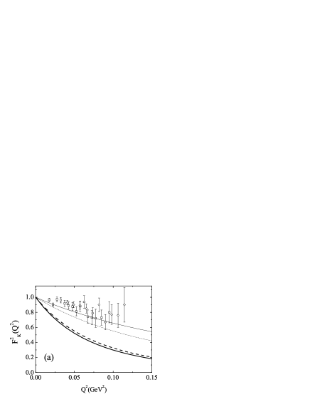
Figure 2: (a) $K$ charge form factor squared in point form as function of $Q^{2}$(GeV²). (b) $K$ charge form factor in point form multiplied by $Q^{2}$. Same description as Fig. 1.

Fig. 2 depicts the $Q^{2}$ behavior of the form factor obtained in point form. The obtained kaon form factor in point form is neither completely off as occurred with the pion nor similar to the results with the other two forms as in the case of the rho. It suggests that with mesons of increasing mass, the form factor improves. This is consistent with one of the conclusions in Ref junhe where it is pointed out that the failure of point form to reproduce the $\pi$ form factor is most likely due to its small mass. Indeed, a small mass indicates large effects due to interactions which we partially neglect when considering the single quark current approximation. Therefore, single quark currents are not enough in point form for low mass mesons.

4.3 Front form

The pion electromagnetic form factor is well described in front form with the simple wave functions considered as can be seen in Fig. 1 of Ref. junhe . The decay constants and charge radii of $\pi$ and $K$ in front form are given in Table 4. The first relevant result is that, with the same ground state wave function that permitted a description of the $\pi$ and $\rho$ form factors, reasonable values for the decay constants and charge radii of the $K$ are obtained. The disagreement with experimental data is less than 10 $\%$ in the decay constants and charge radii with both shapes of the wave function. The overall agreement with experimental data can be slightly improved by considering a little larger size parameter, $b$ from 600 MeV to 650 MeV in the rational case and from 450 MeV to 500 MeV in the gaussian case, as is shown in brackets in the table.

w.f.	$f_{\pi}$ [MeV]	$f_{K}$ [MeV]	$\sqrt{\langle r^{2}_{\pi}\rangle}\ [$fm$]$	$\langle r^{2}_{K^{\pm}}\rangle\ [$fm${}^{2}]$	$\langle r^{2}_{K^{0}}\rangle\ [$fm${}^{2}]$
Rational	98.6 [102.5]	114.0 [119.4]	0.659 [0.679]	0.43 [0.38]	$-$0.080 [$-$0.069]
Gaussian	92.2 [97.2]	106.2 [113.0]	0.665 [0.630]	0.43 [0.36]	$-$0.077 [$-$0.062]
Exp.	92.4 $\pm 0.33$	113.0 $\pm 1.3$	0.663 $\pm 0.006$	0.34 $\pm 0.05$	$-$0.076$\pm$ 0.018

Table 4: Decay constants and charge radii of $\pi$ and $K$ mesons in front form. Same description as Table. 2.

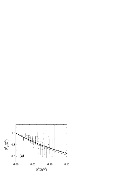
Figure 3: (a) $K$ charge form factor squared in front form as function of $Q^{2}$(GeV²). (b) $K$ charge form factor multiplied by $Q^{2}$. Same description as Fig. 1.

The results with the two sets of parameters are similar and the available experimental data are correctly reproduced. The high-$Q^{2}$ behavior can thus be considered as the front form prediction once the parameters of the wave function were already fixed. These results are similar to other front-form results Cardarelli ; ChoiKaon . The high-$Q^{2}$ behavior is close to $\propto 1/Q^{2}$ for the $K^{0}$ case as occurred in the instant form case. However, as happened with the $\rho$ form factors junhe the fall off of the $K^{+}$ is faster than $\propto 1/Q^{2}$.

5 Form factors and decay constant of the $K^{*}(892)$

The decay constant and electromagnetic form factor of the $K^{*}(892)$ are presented using the three forms of kinematics.

In Table 5 the decay constant of $\rho$ and $K^{*}(892)$ are presented. They have been obtained using the parameters in Table 1, the ones in brackets have been obtained with the readjusted parameters.

	wave function	$f_{\rho}$ [MeV]	$f_{K^{*}(892)}$ [MeV]	$f_{K^{*}(892)}/f_{\rho}$
Instant Form	Gaussian	88.2[128.2]	97.4 [125.3]	1.10[0.98]
	Rational	96.1[129.1]	94.9 [124.5]	0.99[0.96]
Point Form	Gaussian	1842.1	1727.4	0.94
	Rational	5.952$\times 10^{6}$	5.505$\times 10^{6}$	0.92
Front Form	Gaussian	151.3 [168.3]	153.1 [170.5]	1.01 [1.01]
	Rational	175.4 [190.1]	177.6 [192.6]	1.01 [1.01]
EXP		152.8	159.3	1.04

Table 5: Decay constants and charge radii of $\rho$ and $K^{*}(892)$ mesons in instant, point and front forms. The point form values using the readjusted parameters are the same as the instant form values with the same parameters.

First, we note that with all the forms $f_{K^{*}(892)}/f_{\rho}\approx 1$ regardless of the values obtained for each of the decay constants. In particular, the point form values are badly wrong with the original set of parameters, similarly to what was observed in Table 3 for the $\pi$ and $\rho$. If the readjusted set of parameters is used in point form the obtained values would be the same as the instant form ones.

The values quoted as experimental in the Table are taken from Refs. Ivanov ; Maris . The decay constant, $g_{\rho}$, which enters in the process $\rho^{0}\rightarrow e^{+}e^{-}$, is obtained from the matrix element:

$$\frac{M_{\rho}^{2}}{g_{\rho}}\epsilon^{\lambda}_{\mu}(p)=\langle 0|\bar{u}\gamma_{\mu}u|\rho^{0}_{\lambda}(p)\rangle=\frac{1}{\sqrt{2}}\langle 0|\bar{u}\gamma_{\mu}d|\rho^{-}_{\lambda}(p)\rangle\,,$$ (24)

so that

$$f_{\rho}=\frac{M_{\rho}}{g_{\rho}}\,.$$ (25)

The experimental decay width for that channel, 6.77 keV PDG , leads to the value $g_{\rho}=5.03$, that corresponds to $f_{\rho}$=152.8 MeV.

From the partial decay widths of the processes $\tau\to V\nu_{\tau}$ Maris et al. extract the ratio $f_{K^{*}(892)}/f_{\rho}=1.04$. Which implies $f_{K*}=159.3$ MeV (which is comparable to the result of Ref. Jaus , $f_{K*}=153$ MeV).

The instant form calculation (with both the original and the readjusted parameters) underestimates the decay constants by at least 20$\%$. However, the predicted ratios $f_{\pi}/f_{\rho}$ and $f_{K}/f_{K^{*}(892)}$ are in better agreement with experimental data than their nonrelativistic counterparts which are given at the end of Sect 3.

The front form results are in better agreement with the values extracted from experiment specially for the gaussian case. The readjusted parameters do not improve the results in this case.

The electromagnetic form factors of the $K^{*}(892)$ have also been evaluated. In Fig. 4 the coulomb, magnetic and dipole form factors of the $K^{*+}(892)$ are shown calculated making use of Eqs. (13) in the three different forms with the parameters in Table 1.

Qualitatively the obtained form factors are quite similar to the $\rho$ form factors presented in junhe . In fact, as was already reported for the nucleon form factors Riska04 and also for the charge form factor of the $\rho$, a node is found in the charge form factor of the $K^{*+}(892)$ in front form. The node is in this case at $Q^{2}$ around 6 GeV². The predicted behavior for $G_{M}$ is similar in instant and front forms, being considerably smaller in point form.

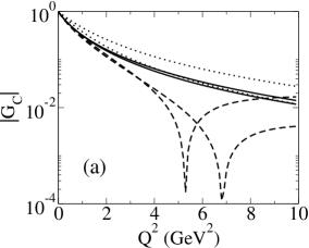
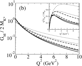
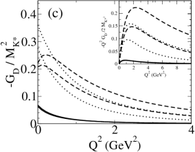
Figure 4: Electromagnetic form factor of the $K^{*}(892)$ obtained in the different forms of kinematics using gaussian wave functions. Solid, dotted and dashed lines stand for instant, point and front form of relativistic kinematics. (a), (b) and (c) show the coulomb, magnetic and dipole form factors, respectively.

The relativistic nature of the calculation produces non-zero values for the charge form factors of the $K^{*0}(892)$ even in the $SU(3)_{f}$ symmetric case. However, the relativistic effect alone is much smaller than the effect arising from the actual existing mass difference between the $s$ and $u(d)$ quarks. In Fig. 5 the charge form factor of the $K^{*0}(892)$ is presented.

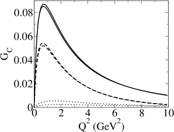
Figure 5: Coulomb form factor of the $K^{*0}(892)$ obtained in the different forms of kinematics using gaussian wave functions. Solid, dotted and dashed lines stand for instant, point and front form of relativistic kinematics.

Finally, as is well known Coester92 ; Keister the use of single quark currents does not permit an unambiguous extraction of the form factors in front form from the considered matrix elements. In this work the form factors are extracted from the same matrix elements as used in Ref. Chung for the case of the deuteron. There, due partly to the large mass of the deuteron as compared to that of the constituents, the breaking in rotational symmetry due to the fact that single quark currents were employed was small. This can be estimated by showing what is called the “angular condition”. This is a certain linear combination of the four matrix elements used to extract the form factors which should vanish would the calculation be rotationally invariant. It can be defined as,

$$\Delta(Q^{2})=(1+2\eta)I_{1,1}+I_{1,-1}-\sqrt{8\eta}I_{1,0}-I_{0,0}\,.$$ (26)

In Fig. 6 the function $\Delta(Q^{2})$ is shown as function of $Q^{2}$ together with the matrix element $I_{1,1}$ which should serve to compare the magnitude of the angular condition. This figure shows that above a certain $Q^{2}$ the obtained behavior of the form factors of spin 1 systems in front form using single quark currents should be taken with care.

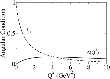
Figure 6: In solid the angular condition defined in Eq. (26), dashed corresponds to the matrix element $\langle 1|I^{+}(0)|1\rangle$. Both for the case of the $K^{*}(892)$.

6 Discussion and summary

In the quark model the main difference between ($\pi$,$\rho$) and ($K$,$K^{*}(892)$) is the substitution of a light quark by a strange quark in the latter. Thus it is natural to explore the ($K$,$K^{*}(892)$) system using the mass operator, which was originally fixed to reproduce the $\pi$ charge form factor, as starting point.

We have presented charge form factors, charge radii and decay constants of the $\pi$, $K$ and $K^{*}(892)$ making use of the three different forms of relativistic kinematics.

In front form, in the impulse approximation and with simple wave functions, the charge form factors, charge radii and decay constants of the $\pi$, $K$ and $K^{*}(892)$ are reasonably reproduced making use of the same parameters that were employed previously to study the $\rho$ form factors. An effective way to phenomenologically account for the differences arising from the presence of a $s$ quark would be to allow for a variation of the mass operator. This is achieved by considering a slightly different set of parameters for the ($K$, $K^{*}$) system. In the front form case, however, the agreement with the data is already acceptable with the original set.

In instant form a slightly worse description of the data is achieved, specially in the case of the vector meson decay constants which are underestimated by 30 $\%$. An improved description of the data can be achieved if two different sets of parameters, one for the mesons made up of light quarks, $\pi$ and $\rho$, and another one for the mesons which contain a strange quark, $K$ and $K^{*}(892)$, is employed. The readjusted values which essentially correspond to a more compact wave function in coordinate space imply a smaller radius for the systems containing an $s$ quark.

The description of the data using point form is very poor.

The approach followed here, used also in Ref. junhe , tries to assess to what extend the existing data for meson form factors can be reproduced using simple assumptions for the mass operator and current operators using the different forms of relativistic quantum mechanics. The results presented here together with other recent ones, e.g., Desplanques0407074 ; Riska04 show that the standard realization of the front form, $Q^{+}=0$, tends to give results which are closer to experimental data. The instant form results are also qualitatively similar. Thus, one can legitimately wonder why the point form fails. Ref. Desplanques0407074 deals with this very question and finds that a common feature which is shared by the “successful” implementations is the fact that in all cases momenta is conserved at the interaction vertex. The point form, and also front form in the $Q^{+}\neq 0$ frame, do not conserve momenta at the quark interaction vertex, which could indicate that the requirement of translation invariance at the quark level would be a much more relevant one. Our work does not contradict those lines.

The same prediction for the high-$Q^{2}$ behavior of the form factor of the $K^{0}$ is found with both instant and front forms. The predicted behavior is close to the QCD prediction of Refs. Farrar . For the charged kaon the high-$Q^{2}$ behavior of the form factors is closer to $\propto 1/Q^{4}$ that to $1/Q^{2}$ both in instant and front forms. The disagreement with the asymptotic QCD behavior may be due to the simple assumptions for the electromagnetic current or simply to the fact that pQCD is not reached as such momentum transfers in this specific problem. In the front form case some care must be taken when considering the form factors of spin-1 mesons. The ambiguity arising when working with single quark currents in the definition of the form factors becomes relevant for low mass systems.

The ratio $f_{\pi}/f_{\rho}$ is considerably improved when relativity is taken into account, as compared to the nonrelativistic results. Although the values for the decay constants for $K^{*}(892)$ are not close to the experimental data in all the forms, it is found that the $f_{K^{*}(892)}/f_{\rho}$ is well reproduced with each of them.

Similar to what was found when studying the form factors of the nucleon and the $\rho$, the charge form factor of the $K^{*}(892)$ in front form contains a node close to 6 GeV². This node could, unlike the one in the nucleon electric form factor, disappear when two body currents are incorporated in the framework.

- (1) P. A. M. Dirac, Rev. Mod. Phys. 49, 392 (1949).
- (2) B. D. Keister and W. N. Polyzou, Adv. Nucl. Phys. 20 (1991) 225.
- (3) Jun He, B. Juliá-Díaz, Yu-bing Dong, Phys. Lett. B 602, 212 (2004).
- (4) P. L. Chung, F. Coester and W. N. Polyzou, Phys. Lett. B 205, 545 (1988); F. Coester and W. N. Polyzou, nucl-th/0405082.
- (5) F. Cardarelli, E. Pace, G. Salme and S. Simula, Phys. Lett. B 357, 267 (1995); F. Cardarelli et. al., Phys. Rev. D 53, 6682 (1996).
- (6) Ho-Meoyng Choi and Chueng-Ryong Ji, Phys. Rev. D 59, 074015 (1999).
- (7) Bo-Wen Xiao, Xin Qian, Bo-Qiang Ma, Eur. Phys. J. A 15, 523 (2002).
- (8) A. F. Krutov and V. E. Troitsky, Phys. Rev. C 65, 045501 (2002).
- (9) A. Amghar, B. Desplanques and L. Theussl, Phys. Lett. B 574, 201 (2003).
- (10) R. F. Wagenbrunn, et. al., Phys. Lett. B 511, 33 (2001).
- (11) B. Juliá-Díaz, D. O. Riska, F. Coester, Phys. Rev. C 69, 035212 (2004).
- (12) B. Desplanques, L. Theußl, Eur. Phys. J. A 13, 461 (2002).
- (13) B. Desplanques, Nucl. Phys. A 748 139 (2005).
- (14) F. E. Close, (AP, London, 1979c.).
- (15) P. L. Chung , Phys. Rev. C 37, 2000 (1988).
- (16) W. Jaus, Phys. Rev. D 67, 094010 (2003).
- (17) F. Cardarelli et. al., Phys. Lett. B 332, 1 (1994).
- (18) D. Ebert, R. N. Faustov and V.O. Galkin, Mod. Phys. Lett.A 17, 803 (2002).
- (19) Particle Data Group, Phys. Lett. B 592, 1 (2004).
- (20) S. R. Amendolia et. al., Nucl. Phys. B 277, 168 (1986).
- (21) S. R. Amendolia et. al., Phys. Lett. B 178, 435 (1986).
- (22) E. B. Dally et. al., Phys. Rev. Lett. 45, 232 (1980).
- (23) G. R. Farrar and D. R. Jackson, Phys. Rev. Lett. 43, 246 (1979).
- (24) B. Desplanques, nucl-th/0407074.
- (25) M. A. Ivanov, Yu. L. Kalinovsky and C. D. Roberts, Phys. Rev. D 60, 034018 (1999).
- (26) Pieter Maris, Peter C. Tandy, Phys. Rev. C 60, 055214 (1999).
- (27) F. Coester, Prog. Part. Nucl. Phys. 29, 1 (1992).
- (28) B. D. Keister, Phys. Rev. D 49, 1500 (1994).