Equilibration in $\varphi^{4}$ theory in 3+1 dimensions

Abstract

The process of equilibration in $\varphi^{4}$ theory is investigated for a homogeneous system in 3+1 dimensions and a variety of out-of-equilibrium initial conditions, both in the symmetric and broken phase, by means of the 2PI effective action. Two $\Phi$-derivable approximations including scattering effects are used: the two-loop and the “basketball”, the latter corresponding to the truncation of the 2PI effective action at $\mathcal{O}(\lambda^{2})$. The approach to equilibrium, as well as the kinetic and chemical equilibration is investigated.

I Introduction

The approach to equilibrium is an important aspect of non-equilibrium dynamics. In the context of particle physics, a large part of the interest derives from results of heavy-ion collision experiments with the RHIC at Brookhaven. The hydrodynamic description of the experiments suggests that there is early thermalization Heinz:2001xi , but a short thermalization time seems to contradict traditional perturbative estimates Baier:2000sb ; Molnar:2001ux . This puzzle has been analyzed in terms of prethermalization Berges:2004ce , and led to further study of the microscopic dynamical processes responsible for the equilibration of the quark-gluon plasma Romatschke:2003ms; Arnold:2004ih ; Arnold:2004ti ; Rebhan:2004ur. Understanding the dynamical processes leading to equilibration in theories with simpler interactions may also shed some light on this issue. We focus in this paper on the case of scalar $\varphi^{4}$ theory.

An adequate method to study out-of-equilibrium dynamics from first principles is the closed-time-path formalism Schwinger:1951ex ; Bakshi:1963 ; Bakshi:1963v2 ; Keldysh:1964 . This scheme leads to causal equations of motion for the various correlation functions that describe their time evolution. The initial conditions are specified by a density matrix, which can be far from equilibrium. Most applications of this method have focused on the study of the equations of motion for the 1- and 2-point functions, known as the Kadanoff-Baym equations KadanoffBaym . Close enough to equilibrium, where kinetic theory is applicable, the Kadanoff-Baym equations have been used extensively, mostly in connection with the study of transport phenomena and the derivation of effective Boltzmann equations (see, for instance Danielewicz:1984kk ; Chou:1985 ; Calzetta:1988cq ; Mrowczynski:1990bu ; Greiner:1998vd ; Blaizot:2001nr and references therein).

Far from equilibrium, kinetic theory is no longer valid, and simple perturbation theory approaches fail to work due to the appearance of secular terms (see for instance Cooper:1996bn ) and/or pinch singularities Altherr:1994fx . These problems are usually absent if one makes use of a self-consistent method, such as the Hartree approximation. Unfortunately, real-time Hartree descriptions do not include sufficient scattering between the field modes, and thus fail to describe the approach to equilibrium. They are also not “universal”, in the sense that the memory from the initial configuration is not completely lost Aarts:2000wi . An infinite number of conserved charges appear that prevent the system from reaching a universal equilibrium state, independently of the initial conditions. However, a Hartree ensemble approximation has been formulated to give an improved description of the early approach to equilibrium Salle:2000hd ; Salle:2002fu .

When the particle occupation numbers are large, another useful method far from equilibrium is the classical approximation. Interesting situations where this occurs include preheating after cosmological inflation due to parametric resonance Boyanovsky:1996sq ; Khlebnikov:1997zt ; Kofman:1997yn ; Garcia-Bellido:1998wm or spinodal decomposition, Boyanovsky:1995me ; Boyanovsky:1996sq ; Felder:2000hj ; Felder:2001kt ; Skullerud:2003ki ; Arrizabalaga:2004iw as well as the early stages of a heavy-ion collision Krasnitz:1998ns ; Krasnitz:1999wc ; Krasnitz:2001qu ; Lappi:2003bi , where the gluon occupation numbers are as large as $\sim 1/\alpha_{s}$, up to a saturation scale Mueller:1999wm ; Baier:2000sb . The classical approximation is not good for describing quantum equilibration, since the system does not move towards the quantum, but to the classical equilibrium state. Nevertheless, the classical theory has been used to shed some light on the dynamics of equilibration and relaxation Aarts:1998kp ; Aarts:1999zn ; Aarts:2000mg ; Boyanovsky:2003tc ; Skullerud:2003ki , as well as a testground for comparison with various other approximation schemes Aarts:2000wi ; Aarts:2001yn ; Blagoev:2001ze ; Arrizabalaga:2004iw .

A powerful scheme that takes into account both scattering and quantum effects is the two-particle irreducible (2PI) effective action Cornwall:1974vz ; Calzetta:1988cq ; Berges:2000ur . The 2PI effective action furnishes a complete representation of the theory in terms of the dressed 1- and 2- point functions. The exact equations of motion describing the time evolution of these correlation functions are obtained by a variational principle on the 2PI effective action functional. Various approximations to the equations of motion can be obtained if one applies the variational method to a truncated version of the action. By construction, these are self-consistent and thus free of secular problems. The approximation can be improved, in principle, by truncating the 2PI effective action at higher order in some expansion parameter.

The main advantages of the 2PI effective action approach stem from the fact that the approximations are performed on the level of a functional. For that reason the approximations have also been called Functional-derivable, or $\Phi$-derivable. The 2PI effective action functional (and any truncation thereof) is, by construction, invariant under global transformations of the 1- and 2-point functions. The variational procedure on any truncation guarantees that the global symmetries are still preserved by the equations of motion. Their associated Noether currents are thus conserved. In particular, this implies that the derived equations of motion conserve energy, as well as global charges Baymconserve ; Ivanov:1998nv ; Bedingham:2003jt . This is a very important feature when studying out-of-equilibrium processes, where most other quantities evolve in complicated ways. The $\Phi$-derivable approximations to the 2PI effective action constitute thus a very convenient method for studying equilibration.

In recent years, approximations based on the 2PI effective action have been applied succesfully to the study of non-equilibrium real-time dynamics. In the context of scalar theories, studies of equilibration have been carried out in the 3-loop $\Phi$-derivable approximation for $\varphi^{4}$ theory, in the symmetric phase, both in 1+1 Berges:2000ur ; Aarts:2001qa and 2+1 dimensions Juchem:2003bi . In the broken phase, the case of 1+1 dimensions has also been discussed in Cooper:2002ze ; Cooper:2002qd . Similar studies of thermalization have been performed in the $O(N)$ model in 1+1 dimensions, both at next-to-leading (NLO) order in a $1/N$ expansion Berges:2001fi ; Aarts:2002dj , and in the bare vertex approximation Cooper:2002ze ; Cooper:2002qd ; Mihaila:2003mh . All these analyses, which include scattering, show that the system indeed equilibrates, with the equilibrium state independent of the initial conditions. Comparing with the loop expansion, the $1/N$ expansion has the advantage that it is applicable in situations where large particle numbers are generated. This has allowed the study of interesting phenomena, such as parametric resonance Berges:2002cz or spinodal decomposition during a phase transition Arrizabalaga:2004iw . The studies in Berges:2002cz and Arrizabalaga:2004iw were done for the $O(N)$ model at NLO, in 3+1 dimensions. Methods based on the 2PI effective action have also been applied to theories with fermions, in 3+1 dimensions Berges:2002wr ; Berges:2004ce . The extension of the 2PI effective action methods for gauge theories, however, is not straightforward due to a residual dependence on the choice of gauge condition Arrizabalaga:2002hn ; Carrington:2003ut ; Calzetta:2004sh ; Andersen:2004re.

In this paper, we use the loop-expansion of the 2PI effective action to study the approach to equilibrium for the case of a real scalar $\varphi^{4}$ theory in 3+1 dimensions, both in the symmetric and broken phase, complementing in this manner the investigations in Berges:2000ur ; Cooper:2002qd ; Juchem:2003bi .

II 2PI loop expansion of $\varphi^{4}$ theory

For $\varphi^{4}$ theory we write the action as

$$S[\varphi]=\int_{\mathcal{C}}d^{4}x\,\left[\frac{1}{2}\partial_{\mu}\varphi(x)\partial^{\mu}\varphi(x)-\frac{1}{2}m^{2}\varphi(x)^{2}-\frac{\lambda}{4!}\varphi(x)^{4}\right],$$ (1)

The subscript $\mathcal{C}$ indicates that the integrations are performed along the real-time Schwinger-Keldysh contour, running from an initial time $t_{0}$ to time $t$ along $\mathcal{C}_{+}$ and going back to $t_{0}$ along $\mathcal{C}_{-}$ (see Fig. 1). The formulation of the theory along the real-time contour $\mathcal{C}$ is appropiate for studying non-equilibrium problems Schwinger:1961 ; Keldysh:1964 ; Chou:1985 .

The system can be in two distinct phases: the symmetric phase (the vacuum field expectation value $v$ is $v=0$) which occurs for $m^{2}>0$, and the broken phase ($v\neq 0$) for $m^{2}<0$. At tree level, the vacuum expectation value in the broken phase is given by $v_{\mbox{\scriptsize tree}}=\sqrt{6|m^{2}|/\lambda}$.

Figure 1: Schwinger-Keldysh contour.

The complete information about the theory can be written in terms of the 2PI effective action, which depends explicitly on the full connected 1- and 2-point functions $\phi(x)\equiv\langle\varphi(x)\rangle$ and $G(x,y)\equiv\langle T_{\mathcal{C}}\varphi(x)\,\varphi(y)\rangle-\phi(x)\phi(y)$. For scalar $\lambda\varphi^{4}$ theory, the 2PI effective action functional can be written as Cornwall:1974vz

$$\Gamma[\phi,G]=S[\phi]-\frac{i}{2}\mbox{Tr}\ln G+\frac{i}{2}\mbox{Tr}\Big{[}(G_{0}^{-1}-G^{-1})\cdot G\Big{]}+\Phi[\phi,G],$$ (2)

with

$$iG_{0}^{-1}(x,y)=\frac{\delta^{2}S[\phi]}{\delta\phi(x)\delta\phi(y)}=\left(-\partial_{x}^{2}-m^{2}-\frac{\lambda}{2}\phi(x)^{2}\right)\delta_{\mathcal{C}}(x,y).$$ (3)

The contour delta function $\delta_{\mathcal{C}}(x,y)$ is given by

$$\delta_{\mathcal{C}}(x,y)=\begin{cases}1&\mbox{if $x=y$ and ${x,y}\in\mathcal{C}_{+}$,}\\ -1&\mbox{if $x=y$ and ${x,y}\in\mathcal{C}_{-}$,}\\ 0&\mbox{otherwise.}\end{cases}$$ (4)

The functional $\Phi$ comprises the sum of the closed two-particle-irreducible (2PI) skeleton diagrams. Up to three loops it is given by

$$i\Phi[\phi,G]=\frac{1}{8}\;\parbox[c]{20.0pt}{\begin{picture}(20.0,30.0)(0.0,0.0) \put(0.0,0.0){} \put(0.0,0.0){} \put(0.0,0.0){} \end{picture}}\;+\frac{1}{12}\;\parbox[c]{45.0pt}{\begin{picture}(45.0,30.0)(0.0,0.0) \put(0.0,0.0){} \put(0.0,0.0){} \put(0.0,0.0){} \put(0.0,0.0){} \put(0.0,0.0){} \put(0.0,0.0){} \put(0.0,0.0){} \put(0.0,0.0){} \end{picture}}\;+\frac{1}{48}\;\parbox[c]{30.0pt}{\begin{picture}(30.0,30.0)(0.0,0.0) \put(0.0,0.0){} \put(0.0,0.0){} \put(0.0,0.0){} \put(0.0,0.0){} \end{picture}}\;+\frac{1}{24}\;\parbox[c]{60.0pt}{\begin{picture}(60.0,30.0)(0.0,0.0) \put(0.0,0.0){} \put(0.0,0.0){} \put(0.0,0.0){} \put(0.0,0.0){} \put(0.0,0.0){} \put(0.0,0.0){} \put(0.0,0.0){} \put(0.0,0.0){} \put(0.0,0.0){} \put(0.0,0.0){} \put(0.0,0.0){} \put(0.0,0.0){} \end{picture}}\;+\frac{1}{24}\parbox[c]{40.0pt}{\begin{picture}(40.0,40.0)(0.0,0.0) \put(0.0,0.0){} \put(0.0,0.0){} \put(0.0,0.0){} \put(0.0,0.0){} \put(0.0,0.0){} \put(0.0,0.0){} \put(0.0,0.0){} \put(0.0,0.0){} \put(0.0,0.0){} \put(0.0,0.0){} \put(0.0,0.0){} \put(0.0,0.0){} \end{picture}}.$$ (5)

The Feynman rules for these diagrams are given by

$$\;\parbox[c]{20.0pt}{\begin{picture}(20.0,30.0)(0.0,0.0) \put(0.0,0.0){} \put(0.0,0.0){} \put(0.0,0.0){} \end{picture}}\;=-i\lambda,\qquad\;\parbox[c]{30.0pt}{\begin{picture}(30.0,30.0)(0.0,0.0) \put(0.0,0.0){} \raise 8.0pt\hbox to0.0pt{\kern 0.0pt\makebox(0.0,0.0)[ct]{${\mbox{\scriptsize$x$}}$}\hss} \ignorespaces \raise 8.0pt\hbox to0.0pt{\kern 30.0pt\makebox(0.0,0.0)[ct]{${\mbox{\scriptsize$y$}}$}\hss} \ignorespaces \end{picture}}\;=G(x,y),\qquad\;\parbox[c]{30.0pt}{\begin{picture}(30.0,30.0)(0.0,0.0) \put(0.0,0.0){} \raise 8.0pt\hbox to0.0pt{\kern 5.0pt\makebox(0.0,0.0)[ct]{${\mbox{\scriptsize$x$}}$}\hss} \ignorespaces \put(0.0,0.0){} \put(0.0,0.0){} \end{picture}}\;=\phi(x).$$ (6)

In this manner, the functional $\Phi[\phi,G]$ is

$$\Phi[\phi,G]=-\frac{\lambda}{8}\int_{\mathcal{C}}d^{4}x\;G(x,x)^{2}+i\frac{\lambda^{2}}{12}\int_{\mathcal{C}}d^{4}x\int_{\mathcal{C}}d^{4}y\;\phi(x)G(x,y)^{3}\phi(y)+i\frac{\lambda^{2}}{48}\int_{\mathcal{C}}d^{4}x\int_{\mathcal{C}}d^{4}y\;G(x,y)^{4}+\ldots$$ (7)

The 2PI effective action $\Gamma[\phi,G]$ provides an exact representation of the full theory. Considering only a finite number of terms in the series of diagrams in $\Phi$ leads to a truncated action, from which approximate “physical” 1- and 2-point functions can be obtained by a variational procedure. As a result of this, a resummation of effects from higher orders in perturbation theory is performed.

In this paper we shall investigate the truncations of the 2PI effective action up to three loops, in particular up to ${\mathcal{O}}(\lambda^{2})$. The various truncations considered and their corresponding truncated functionals $\Phi_{\mbox{\scriptsize tr}}$ are displayed in table 1. The organization of the truncations discussed is based on the superficial counting of loops and/or vertices in the diagrams of $\Phi$, i.e. no assumption is taken on the coupling constant dependence of $\phi$ or $G$.

Truncation	Order	$i\Phi_{\mbox{\tiny tr}}[\phi,G]$
Hartree approximation	${\mathcal{O}}(\lambda)$	$\parbox[c]{1.0pt}{\begin{picture}(1.0,25.0)(0.0,0.0) \end{picture}}\par\frac{1}{8}\parbox[c]{20.0pt}{\begin{picture}(20.0,20.0)(0.0,0.0) \put(0.0,0.0){} \put(0.0,0.0){} \put(0.0,0.0){} \end{picture}}$
Two-loop approximation	2 loops	$\parbox[c]{1.0pt}{\begin{picture}(1.0,25.0)(0.0,0.0) \end{picture}}\par\frac{1}{8}\parbox[c]{20.0pt}{\begin{picture}(20.0,20.0)(0.0,0.0) \put(0.0,0.0){} \put(0.0,0.0){} \put(0.0,0.0){} \end{picture}}+\frac{1}{12}\;\parbox[c]{30.0pt}{\begin{picture}(30.0,20.0)(0.0,0.0) \put(0.0,0.0){} \put(0.0,0.0){} \put(0.0,0.0){} \put(0.0,0.0){} \put(0.0,0.0){} \put(0.0,0.0){} \put(0.0,0.0){} \put(0.0,0.0){} \end{picture}}$
“Basketball” approximation	${\mathcal{O}}(\lambda^{2})$	$\parbox[c]{1.0pt}{\begin{picture}(1.0,25.0)(0.0,0.0) \end{picture}}\par\frac{1}{8}\parbox[c]{20.0pt}{\begin{picture}(20.0,20.0)(0.0,0.0) \put(0.0,0.0){} \put(0.0,0.0){} \put(0.0,0.0){} \end{picture}}+\frac{1}{12}\;\parbox[c]{30.0pt}{\begin{picture}(30.0,20.0)(0.0,0.0) \put(0.0,0.0){} \put(0.0,0.0){} \put(0.0,0.0){} \put(0.0,0.0){} \put(0.0,0.0){} \put(0.0,0.0){} \put(0.0,0.0){} \put(0.0,0.0){} \end{picture}}+\frac{1}{48}\;\parbox[c]{30.0pt}{\begin{picture}(20.0,20.0)(0.0,0.0) \put(0.0,0.0){} \put(0.0,0.0){} \put(0.0,0.0){} \put(0.0,0.0){} \end{picture}}$

Table 1: Truncations of the 2PI effective action.

In our analysis using the three-loop “basketball approximation” we have neglected the other three-loop diagrams

$$\;\parbox[c]{60.0pt}{\begin{picture}(60.0,30.0)(0.0,0.0) \put(0.0,0.0){} \put(0.0,0.0){} \put(0.0,0.0){} \put(0.0,0.0){} \put(0.0,0.0){} \put(0.0,0.0){} \put(0.0,0.0){} \put(0.0,0.0){} \put(0.0,0.0){} \put(0.0,0.0){} \put(0.0,0.0){} \put(0.0,0.0){} \end{picture}}\;\quad,\quad\parbox[c]{40.0pt}{\begin{picture}(40.0,40.0)(0.0,0.0) \put(0.0,0.0){} \put(0.0,0.0){} \put(0.0,0.0){} \put(0.0,0.0){} \put(0.0,0.0){} \put(0.0,0.0){} \put(0.0,0.0){} \put(0.0,0.0){} \put(0.0,0.0){} \put(0.0,0.0){} \put(0.0,0.0){} \put(0.0,0.0){} \end{picture}}.$$ (8)

These diagrams are respectively of superficial order $\mathcal{O}(\lambda^{3}\phi^{2})$ and $\mathcal{O}(\lambda^{4}\phi^{4})$. In the symmetric phase, where $\phi\sim 0$, they can be safely neglected. In the broken phase, however, $\phi\sim v_{\mbox{\scriptsize tree}}\sim\mathcal{O}(\lambda^{-1/2})$ and thus both diagrams become $\mathcal{O}(\lambda^{2})$. In this situation it is not clear whether these contributions can be ignored. Due to the difficulty in treating the above diagrams numerically, we decided to neglect them in our analysis. Part of the first diagram in (8) can be recovered at NLO in a $1/N$-expansion Aarts:2002dj .

III Equations of motion

In the formulation on the real-time contour ${\mathcal{C}}$, a $\Phi$-derivable approximation to the 2PI effective action $\Gamma$ leads to equations of motion for the 1- and 2-point functions. Indeed, solving the stationarity conditions

$$\frac{\delta\Gamma[\phi,G]}{\delta\phi}=0,\qquad\frac{\delta\Gamma[\phi,G]}{\delta G}=0,$$ (9)

leads to the equation for the mean field

$$\frac{\delta S[\phi]}{\delta\phi(x)}+\frac{1}{2}\lambda G(x,x)\phi(x)=-\frac{\delta\Phi[\phi,G]}{\delta\phi(x)},$$ (10)

and for the 2-point function

$$\delta_{\mathcal{C}}(x,y)=\int_{\mathcal{C}}d^{4}z\,G_{0}^{-1}(x,z)G(z,y)+i\int_{\mathcal{C}}d^{4}z\,\Sigma(x,z)G(z,y).$$ (11)

The self-energy $\Sigma(x,y)$ is given, in terms of the functional $\Phi$, by

$$\Sigma(x,y)=-2\frac{\delta\Phi[\phi,G]}{\delta G(y,x)}.$$ (12)

To the order considered here, the self-energy $\Sigma$ is determined from the truncated functional $\Phi^{\mbox{\scriptsize tr}}[\phi,G]$. To $\mathcal{O}(\lambda^{2})$ one finds

$$\Sigma[\phi,G]=i\Big{[}\,\frac{1}{2}\;\parbox[c]{25.0pt}{ \begin{picture}(25.0,32.5)(0.0,0.0) \put(0.0,0.0){} \put(0.0,0.0){} \put(0.0,0.0){} \end{picture}}\;+\frac{1}{2}\;\;\parbox[c]{45.0pt}{\begin{picture}(45.0,30.0)(0.0,0.0) \put(0.0,0.0){} \put(0.0,0.0){} \put(0.0,0.0){} \put(0.0,0.0){} \put(0.0,0.0){} \put(0.0,0.0){} \put(0.0,0.0){} \put(0.0,0.0){} \put(0.0,0.0){} \put(0.0,0.0){} \put(0.0,0.0){} \end{picture}}\;\;+\frac{1}{6}\;\;\parbox[c]{45.0pt}{\begin{picture}(45.0,30.0)(0.0,0.0) \put(0.0,0.0){} \put(0.0,0.0){} \put(0.0,0.0){} \put(0.0,0.0){} \end{picture}}\;\;\Big{]}$$ (13)

For the case of the Hartree approximation (see Table 1), only the first diagram in (13) (the “leaf” diagram) enters in $\Sigma$. For the case of the two-loop and “basketball” approximations respectively, the second and third diagrams in (13) (the “eye” and the “sunset”) have to be taken into account. For the study of nonequilibrium dynamics these are important diagrams as they account for scattering and hence can lead to equilibration.

The self-energy can be split up into a local and a nonlocal part,

$$\Sigma(x,y)=\Sigma^{\rm l}(x)\delta_{{\mathcal{C}}}(x,y)+\Sigma^{\rm nl}(x,y),$$ (14)

with

$$\Sigma^{\rm l}(x) =\frac{\lambda}{2}G(x,x),$$ (15)

$$\Sigma^{\rm nl}(x,y) =-i\frac{\lambda^{2}}{2}\phi(x)G(x,y)^{2}\phi(y)-i\frac{\lambda^{2}}{6}G(x,y)^{3}.$$ (16)

The quantities entering in the equations of motion (10) and (11) are defined in the real-time contour $\mathcal{C}$. For the non-local quantities, such as $G(x,y)$ and $\Sigma^{\rm nl}(x,y)$, this implies the appearance of several components, corresponding to the various positions of the time indices along the contour. For $G(x,y)$, the various contour components are written in a compact manner by using the decomposition in terms of the correlators $G^{>}(x,y)\equiv\langle\varphi(x)\varphi(y)\rangle$ and $G^{<}(x,y)\equiv\langle\varphi(y)\varphi(x)\rangle$, namely

$$G(x,y)=\Theta_{\mathcal{C}}(x_{0}-y_{0})G^{>}(x,y)+\Theta_{\mathcal{C}}(y_{0}-x_{0})G^{<}(x,y).$$ (17)

The $\Theta$-functions used here are defined along the contour $\mathcal{C}$. A similar decomposition can be written for the self-energy $\Sigma^{\rm nl}(x,y)$, i.e.

$$\Sigma^{\rm nl}(x,y)=\Theta_{\mathcal{C}}(x_{0}-y_{0})\Sigma^{>}(x,y)+\Theta_{\mathcal{C}}(y_{0}-x_{0})\Sigma^{<}(x,y).$$ (18)

From (17) we see that the dynamics of the propagator is entirely described by the two complex functions $G^{>}$ and $G^{<}$. For the real scalar theory under consideration, these functions satisfy the property $\left[G^{>}(x,y)\right]^{\star}=G^{<}(x,y)$, which leaves only one independent complex function describing the propagator dynamics. This can be parametrized in terms of two real functions $F$ and $\rho$ according to

$$G^{>}(x,y) =F(x,y)-\frac{i}{2}\rho(x,y),$$ (19)

$$G^{<}(x,y) =F(x,y)+\frac{i}{2}\rho(x,y).$$ (20)

The functions $F$ and $\rho$ correspond to the correlators

$$F(x,y) =\frac{1}{2}\left[G^{>}(x,y)+G^{<}(x,y)\right]=\frac{1}{2}\left\langle\left\{\varphi(x),\varphi(y)\right\}\right\rangle,$$ (21)

$$\rho(x,y) =iG^{>}(x,y)-iG^{<}(x,y)=i\left\langle\left[\varphi(x),\varphi(y)\right]\right\rangle.$$ (22)

The correlators $F(x,y)$ and $\rho(x,y)$ contain, respectively, statistical and spectral information about the system. They satisfy the symmetry properties

$$F(x,y) =F(y,x),$$ (23)

$$\rho(x,y) =-\rho(y,x),$$ (24)

which make them very useful for numerical implementation Aarts:2001qa .

For the self-energy we introduce, in a similar fashion, the quantities

$$\Sigma^{F}(x,y) =\frac{i}{2}\left[\Sigma^{>}(x,y)+\Sigma^{<}(x,y)\right],$$ (25)

$$\Sigma^{\rho}(x,y) =\Sigma^{<}(x,y)-\Sigma^{>}(x,y),$$ (26)

which satisfy similar properties as their propagator counterparts. For the case of the non-local part of the self-energy given by (16), these become

$$\Sigma^{F}(x,y) =\frac{\lambda^{2}}{2}\phi(x)\phi(y)\left[F^{2}(x,y)-\frac{\rho^{2}(x,y)}{4}\right]+\frac{\lambda^{2}}{6}F(x,y)\left[F^{2}(x,y)-\frac{3\rho^{2}(x,y)}{4}\right],$$ (27)

$$\Sigma^{\rho}(x,y) =\lambda^{2}\phi(x)\phi(y)\big{[}F(x,y)\rho(x,y)\big{]}+\frac{\lambda^{2}}{6}\rho(x,y)\left[3F^{2}(x,y)-\frac{\rho^{2}(x,y)}{4}\right].$$ (28)

In the study presented here, we shall focus on the dynamics of the statistical and spectral correlators $F$ and $\rho$. Their equations of motion are determined from (11) by using the decompositions (17) and (18), as well as the definitions (21) and (22). For the case $x_{0}>y_{0}$, one finds

$$\left[\partial_{x}^{2}+M^{2}(x)\right]F(x,y) =\int_{0}^{x_{0}}dz_{0}\int d^{3}z\;\Sigma^{\rho}(x,z)F(z,y)-\int_{0}^{y_{0}}dz_{0}\int d^{3}z\;\Sigma^{F}(x,z)\rho(y,z),$$ (29)

$$\left[\partial_{x}^{2}+M^{2}(x)\right]\rho(x,y) =\int_{y_{0}}^{x_{0}}dz_{0}\int d^{3}z\;\Sigma^{\rho}(x,z)\rho(z,y),$$ (30)

with

$$M^{2}(x)=m^{2}+\frac{\lambda}{2}\phi(x)^{2}+\Sigma^{l}(x)=m^{2}+\frac{\lambda}{2}\phi(x)^{2}+\frac{\lambda}{2}F(x,x).$$ (31)

With the same considerations as for the 2-point functions, the equation of motion of the mean field $\phi(x)$ is found from (10) to be

$$\left[\partial_{x}^{2}+M^{2}(x)-\frac{\lambda}{3}\phi(x)^{2}\right]\phi(x)=\int_{0}^{x_{0}}dz_{0}\int d^{3}z\;\widetilde{\Sigma}^{\rho}(x,z)\phi(z),$$ (32)

where $\widetilde{\Sigma}^{\rho}(x,z)$ is the $\rho$-component of the “sunset” self-energy diagram, given by

$$\widetilde{\Sigma}^{\rho}(x,z)=-\frac{\lambda^{2}}{6}\rho(x,z)\left[3F(x,z)^{2}-\frac{\rho(x,z)^{2}}{4}\right].$$ (33)

This contribution derives from including the second of the 2PI diagrams in $\Phi$ (see Eq. 5). Therefore it is present in both the two-loop and “basketball” approximations. The tilde in $\tilde{\Sigma}$ is written to avoid any confusion with the self-energy $\Sigma$ entering in the equations of motion for the propagator. In that case, the “sunset” diagram enters in the self-energy $\Sigma$ only in the “basketball” approximation.

With the self-energies $\Sigma^{F}$, $\Sigma^{\rho}$ and $\widetilde{\Sigma}^{\rho}$ given respectively by (27),(28) and (33), equations (29-32) constitute a set of closed coupled evolution equations for the correlators $F$ and $\rho$ and the mean field $\phi$. These equations are explicitly causal, i.e. the evolution of $F$, $\rho$ and $\phi$ is determined by the values of the correlators and mean fields at previous times. The driving terms in the RHS of those equations consist of nonlocal “memory” integrals that contain the information about the earlier stages of the evolution. By specifying a complete set of initial conditions for $F$, $\rho$ and $\phi$, the equations of motion (29-32) constitute an initial value problem. We perform a numerical analysis of the equations of motion in the next section.

We finish this section with the calculation of the energy density corresponding to the truncations of the 2PI effective action. The energy density is determined from the energy-momentum tensor component $T^{00}$. It takes the form (see appendix A)

$$T^{00}({\mathbf{x}},t) =\frac{1}{2}\Big{[}\partial_{t}\partial_{t^{\prime}}+\partial_{{\mathbf{x}}}\partial_{{\mathbf{x}}^{\prime}}+m^{2}\Big{]}\big{(}F({\mathbf{x}},t;{\mathbf{x}}^{\prime},t^{\prime})+\phi({\mathbf{x}},t)\phi({\mathbf{x}},t^{\prime})\big{)}\bigg{|}_{\begin{subarray}{c}{\mathbf{x}}={\mathbf{x}}^{\prime}\\ t=t^{\prime}\end{subarray}}$$

$$\qquad+\frac{1}{4!}\lambda\phi(\mathbf{x},t)^{4}+\frac{1}{4}\lambda\phi(\mathbf{x},t)^{2}F({\mathbf{x}},t;{\mathbf{x}},t)-\frac{\delta\Phi}{\delta\zeta(x)}\Big{|}_{{\zeta=1}}.$$ (34)

Here $\zeta(x)$ is an auxiliary scale factor introduced in the coupling constant as $\lambda\rightarrow\zeta(x)\lambda$. For a given truncation, the energy density is obtained from (34) by the substitution $\Phi\rightarrow\Phi_{\mbox{\scriptsize tr}}$. In the “basketball” approximation, for instance, the energy density becomes

$$T^{00}({\mathbf{x}},t) =\frac{1}{2}\left[\partial_{t}\phi({\mathbf{x}},t)\right]^{2}+\frac{1}{2}\left[\partial_{{\mathbf{x}}}\phi({\mathbf{x}},t)\cdot\partial_{{\mathbf{x}}}\phi({\mathbf{x}},t)\right]+\frac{1}{2}\partial_{t}\partial_{t^{\prime}}F({\mathbf{x}},t;{\mathbf{x}},t^{\prime})\big{|}_{t=t^{\prime}}+\frac{1}{2}\partial_{{\mathbf{x}}}\cdot\partial_{\mathbf{y}}F({\mathbf{x}},t;{\mathbf{x}},t)\big{|}_{{\mathbf{x}}=\mathbf{y}}$$

$$\ +\frac{1}{2}m^{2}\left[\phi^{2}({\mathbf{x}},t)+F({\mathbf{x}},t;{\mathbf{x}},t)\right]+\frac{1}{4!}\lambda\phi({\mathbf{x}},t)^{4}+\frac{1}{4}\lambda F({\mathbf{x}},t;{\mathbf{x}},t)\phi({\mathbf{x}},t)^{2}+\frac{1}{8}\lambda F({\mathbf{x}},t;{\mathbf{x}},t)^{2}$$

$$+\frac{\lambda^{2}}{6}\int_{0}^{t}dz_{0}\int d^{3}z\;\phi({\mathbf{x}},t)\left[\frac{\rho({\mathbf{x}},t;{\mathbf{z}},z_{0})^{3}}{4}-3\rho({\mathbf{x}},t;{\mathbf{z}},z_{0})F({\mathbf{x}},t;{\mathbf{z}},z_{0})^{2}\right]\,\phi({\mathbf{z}},z_{0})$$

$$+\frac{\lambda^{2}}{6}\int_{0}^{t}dz_{0}\int d^{3}z\;\left[\frac{\rho({\mathbf{x}},t;{\mathbf{z}},z_{0})^{2}}{4}-F({\mathbf{x}},t;{\mathbf{z}},z_{0})^{2}\right]F({\mathbf{x}},t;{\mathbf{z}},z_{0})\rho({\mathbf{x}},t;{\mathbf{z}},z_{0}).$$ (35)

It follows from translational invariance Baymconserve ; Ivanov:1998nv (see also appendix A), that the energy density (35) is exactly conserved in the evolution.

IV Numerical analysis and renormalization

We study the non-equilibrium evolution of the correlators $F$ and $\rho$ and the mean field $\phi$ by solving numerically the equations of motion (29-32), both in the symmetric and the broken phase.

IV.1 Numerical implementation

We shall consider the system to be discretized on a space-time lattice with a finite spatial volume and spatially periodic boundary conditions. The action of $\varphi^{4}$ theory on a space-time lattice is

$$S_{\mbox{\scriptsize lat}}[\varphi]=a^{3}\,a_{t}\sum_{\mathbf{x},t}\left[\frac{1}{2}\left(\partial_{t}\varphi(\mathbf{x},t)\right)^{2}-\frac{1}{2}\sum_{i}\left(\partial_{i}\varphi(\mathbf{x},t)\right)^{2}-\frac{1}{2}m_{0}^{2}\varphi(\mathbf{x},t)^{2}-\frac{1}{4!}\lambda_{0}\varphi(\mathbf{x},t)^{4}\right].$$ (36)

The lattice spacings $a$ and $a_{t}$ correspond to the spatial and time directions, respectively. The derivatives stand for forward finite differences, e.g. $\partial_{t}\varphi(\mathbf{x},t)=(1/a_{t})\left[\varphi(\mathbf{x},t+a_{t})-\varphi(\mathbf{x},t)\right]$. The spatial lattice volume is given in terms of the number of lattice sites $N$ as $V=L^{3}=(Na)^{3}$. In the following we shall use lattice units ($a=1)$ and write $dt=a_{t}/a$ for the dimensionless time-step. The mass $m_{0}$ and coupling $\lambda_{0}$ are bare parameters to be determined below. The lattice version of the squared spatial momentum is given by

$$k_{\mbox{\scriptsize lat}}^{2}=\sum^{3}_{i=1}\left(2-2\cos\mathbf{k}_{i}\right),\quad\mbox{with}\quad\mathbf{k}_{i}=\frac{2\pi n_{i}}{N},\quad n_{i}=-\frac{N}{2}+1,\ldots,\frac{N}{2}\ (\mbox{for $N$ even}).$$ (37)

Plotting data as a function of $k_{\mbox{\scriptsize lat}}^{2}$ corrects for a large part of the lattice artifacts.

The lattice provides a cutoff and regularizes the ultraviolet divergent terms in the continuum limit, which are to be dealt with by renormalization. The continuum renormalization of $\Phi$-derivable approximations has been studied in detail in vanHees:2001ik ; VanHees:2001pf ; Blaizot:2003an ; Berges:2004hn ; Cooper:2004rs . For our purpose it is enough to use an approximate renormalization that ensures that the relevant length scales in our simulations are larger than the lattice spacing $a$. This is achieved by simply choosing the bare paremeters $m_{0}$ and $\lambda_{0}$ according to the one-loop formulas that relate them to the renormalized parameters. The bare mass $m_{0}$ is given in terms of the renormalized mass $m$ by (see also Blaizot:2003an ; Reinosa:2003qa ; mythesis )

$$m_{0}^{2}=m^{2}-\delta m^{2},$$ (38)

with the mass counterterm

$$\delta m^{2}=\frac{\lambda}{2a^{2}}I_{1}(am)-\frac{\lambda^{2}v^{2}}{2a^{2}}I_{2}(am).$$ (39)

The $I_{1}$ and $I_{2}$ in (39) are dimensionless integrals coming respectively from the one-loop “leaf” and “eye” diagrams in the self-energy $\Sigma$ at zero temperature. On the lattice, for continuous time and in the infinite volume limit ($N\rightarrow\infty$), they are given by

$$I_{1}(am) =i\int_{-\pi/a}^{\pi/a}\frac{d^{3}k}{(2\pi)^{3}}\int\frac{dk_{0}}{2\pi}\frac{a^{2}}{k_{0}^{2}-a^{-2}k_{\mbox{\scriptsize lat}}^{2}-m^{2}-i\epsilon}=\int_{-\pi}^{\pi}\frac{d^{3}k}{(2\pi)^{3}}\frac{1}{4\sqrt{\smash[b]{a^{2}m^{2}+k^{2}_{{\mbox{\scriptsize lat}}}}}},$$ (40)

$$I_{2}(am) =i\int_{-\pi/a}^{\pi/a}\frac{d^{3}k}{(2\pi)^{3}}\int\frac{dk_{0}}{2\pi}\left(\frac{1}{k_{0}^{2}-a^{-2}k_{\mbox{\scriptsize lat}}^{2}-m^{2}-i\epsilon}\right)^{2}=\int_{-\pi}^{\pi}\frac{d^{3}k}{(2\pi)^{3}}\frac{1}{8\sqrt{\smash[b]{\left(a^{2}m^{2}+k^{2}_{{\mbox{\scriptsize lat}}}\right)^{3}}}}.$$ (41)

The bare coupling $\lambda_{0}$ can be determined from the one-loop expression (see Blaizot:2003an ; Reinosa:2003qa ; mythesis )

$$\frac{1}{\lambda_{0}}=\frac{1}{\lambda}-I_{2}(am).$$ (42)

The renormalization conditions that define the renormalized mass and coupling via Eqns. (38) and (42) are such that they correspond to the values of the two- and four-point vertex functions at vanishing external momenta. For the values of the couplings ($\lambda=1,6$) and lattice spacing ($0.5<am<1$) that we use in our simulations, the difference between $\lambda_{0}$ and $\lambda$ is less than 10%. In practice, we simply choose $\lambda_{0}$ as if it were the renormalized coupling.

For the renormalization of the mass we use (38), which for the case of a spatial $N^{3}$ lattice is then given by

$$m_{0}^{2}=\pm m^{2}-\frac{\lambda_{0}}{4a^{2}N^{3}}\sum_{\mathbf{k}}\frac{1}{\sqrt{\smash[b]{a^{2}m^{2}+k^{2}_{\mbox{\scriptsize lat}}}}}+\frac{\lambda_{0}^{2}v^{2}}{8a^{2}N^{3}}\sum_{\mathbf{k}}\frac{1}{\sqrt{\smash[b]{\left(a^{2}m^{2}+k^{2}_{\mbox{\scriptsize lat}}\right)^{3}}}}.$$ (43)

In practice, we conveniently choose a value for the renormalized mass (such that $am<1$), which determines via Eq. (43) the bare mass that enters in the equations of motion for the mean field and propagator. In our simulations we used $am=0.7$ and $N=16$. Given the input parameters $m_{0}$ and $\lambda_{0}$, the output physics is of course not known precisely, it is determined by the $\Phi$-derived equations of motion.

IV.2 Initial conditions

We specialize to a spatially homogeneous situation. In this case, $F(x,y)=F(t,t^{\prime},{\bf x-y})$, $\rho(x,y)=\rho(t,t^{\prime},{\bf x-y})$ so we can perform a Fourier transformation and study the propagator modes $\rho_{\mathbf{k}}(t,t^{\prime})$ and $F_{\mathbf{k}}(t,t^{\prime})$. In addition, the mean field depends only on time. To specify the time evolution, the equations of motion (29-32) must be supplemented with initial conditions at $t=t^{\prime}=0$. These are given by the values and derivatives of $\rho$, $F$ and $\phi$ at initial time. The initial conditions for $\rho$ follow from it being the expectation value of the commutator of two fields, which implies

$$\rho_{\mathbf{k}}(t,t)=0,\qquad\partial_{t}\rho_{\mathbf{k}}(t,t^{\prime})\big{|}_{t=t^{\prime}}=1,$$ (44)

Imposing the condition (44) at $t=t^{\prime}=0$, it is preserved by the equations of motion.

For the statistical correlator $F$, we choose initial conditions of the form

$$\langle\{\varphi_{\bf k}(t),\varphi_{\bf-k}(t^{\prime})\}\rangle|_{t=t^{\prime}=0}=F_{\mathbf{k}}(t,t^{\prime})\big{|}_{t=t^{\prime}=0} =\frac{1}{\omega_{\mathbf{k}}}\left[n_{\mathbf{k}}+\frac{1}{2}\right],$$ (45)

$$\langle\{\pi_{\bf k}(t),\varphi_{\bf-k}(t^{\prime})\}\rangle|_{t=t^{\prime}=0}=\partial_{t}F_{\mathbf{k}}(t,t^{\prime})\big{|}_{t=t^{\prime}=0} =0,$$ (46)

$$\langle\{\pi_{\bf k}(t)\pi_{\bf-k}(t^{\prime})\}\rangle|_{t=t^{\prime}=0}=\partial_{t}\partial_{t^{\prime}}F_{\mathbf{k}}(t,t^{\prime})\big{|}_{t=t^{\prime}=0} =\omega_{\mathbf{k}}\left[n_{\mathbf{k}}+\frac{1}{2}\right].$$ (47)

where $\pi_{\mathbf{k}}(t)=\partial_{t}\varphi_{\mathbf{k}}(t)$ are the conjugate field momenta, $n_{\mathbf{k}}$ is some distribution function and $\omega_{\mathbf{k}}=\sqrt{\smash[b]{m_{\rm in}^{2}+\mathbf{k}^{2}}}$, with $m_{\rm in}$ to be specified shortly. An initial condition of this form can be represented by a gaussian density matrix. We will use the following cases for the distribution function $n_{\mathbf{k}}$:

• Thermal: The distribution function $n_{\mathbf{k}}$ corresponds to a Bose-Einstein, at some initial temperature $T_{\mbox{\scriptsize in}}$,

  $$n_{\bf k}=\frac{1}{e^{(\omega_{\bf k}/T_{\rm in})}-1}.$$ (48)

  This also includes the “vacuum” initial condition of $T_{\mbox{\scriptsize in}}=0$ (which is of course only an approximation to the vacuum state in the interacting theory). The input mass for all $T_{\mbox{\scriptsize in}}$ is the renormalized $m_{\rm in}=m$ in the symmetric phase, and $m_{\rm in}=\sqrt{2}m$ in the broken phase. We expect these to be close to the zero-temperature particle masses, respectively in these phases.

• Top-hat: In this case, only modes with momenta within a range ${\mathbf{k}}_{\mbox{\scriptsize min}}^{2}<{\mathbf{k}}^{2}<{\mathbf{k}}^{2}_{\mbox{\scriptsize max}}$ are occupied. The distribution function can be parametrized as

  $$n_{\mathbf{k}}=\eta\,\Theta({\mathbf{k}}^{2}_{\mbox{\scriptsize max}}-{\mathbf{k}}^{2})\Theta({\mathbf{k}}^{2}-{\mathbf{k}}^{2}_{\mbox{\scriptsize min}}),$$ (49)

  where $\eta$ represents the occupancy of the excited modes. The input mass is again given by $m_{\rm in}=m$ (symmetric) and $m_{\rm in}=\sqrt{2}m$ (broken).

The mean field is initialized at $\phi=0$ (“symmetric phase”) and $\phi=v_{\mbox{\scriptsize tree}}$, (the zero temperature “broken phase”). Below, we will also allow the mean field to be slightly displaced from these two, in order to study relaxation in a thermal background.

IV.3 Observables

As the system evolves in time, we expect the scattering processes to lead to equilibration. The occupation numbers of the momentum modes are expected to gradually approach a Bose-Einstein distribution, provided the coupling is not too strong. The statistical information about the evolving system can be extracted from the equal-time correlation function $F_{\mathbf{k}}(t,t)$. We can use $F_{\mathbf{k}}$ to define a quasiparticle distribution function and frequencies as Aarts:1999zn ; Salle:2000hd ; Aarts:2001qa ; Salle:2002fu ; Skullerud:2003ki

$$n_{\mathbf{k}}(t)+\frac{1}{2} =c_{\mathbf{k}}\sqrt{\partial_{t}\partial_{t^{\prime}}F_{\mathbf{k}}(t,t^{\prime})\big{|}_{t=t^{\prime}}\,F_{\mathbf{k}}(t,t)},$$ (50)

$$\omega_{\mathbf{p}}(t) =\sqrt{\frac{\partial_{t}\partial_{t^{\prime}}F_{\mathbf{k}}(t,t^{\prime})\big{|}_{t=t^{\prime}}}{F_{\mathbf{k}}(t,t)}}.$$ (51)

The correction $c_{\mathbf{k}}$ diminishes errors associated with the time discretization on the lattice. It is given by Salle:2002fu

$$c_{\mathbf{k}}=\sqrt{1-\frac{1}{4}dt^{2}\omega_{\mathbf{k}}^{2}}.$$ (52)

Both definitions (50) and (51) are valid for a free field system in equilibrium, and have proven to be very useful in interacting theories out of equilibrium as well Salle:2000hd ; Salle:2000jb ; Skullerud:2003ki ; Salle:2003ju . From the studies in 1+1 and 2+1 dimensions Aarts:2001qa ; Juchem:2003bi , we expect the system to exhibit a quasiparticle structure before reaching thermal equilibrium. The definitions (50) and (51) can be used to monitor the evolution of the system towards such a quasiparticle-like state, and eventually to equilibrium.

Once the system is close to equilibrium, we can read from (51) the effective quasiparticle mass $m_{\mbox{\scriptsize eff}}(t)$ by comparing it to the dispersion relation

$$\omega^{2}_{\mathbf{k}}(t)=c^{2}(t)\left(m_{\mbox{\scriptsize eff}}^{2}(t)+{\mathbf{k}}^{2}\right),$$ (53)

where the factor $c(t)$ is a measure of an effective speed of light or an inverse refractive index. A temperature $T_{\mbox{\scriptsize eff}}(t)$ and chemical potential $\mu_{\mbox{\scriptsize eff}}(t)$ can be determined by fitting the occupation number (50) to a Bose-Einstein distribution

$$n_{\mathbf{p}}(t)=\frac{1}{e^{\left[\omega_{\mathbf{p}}(t)-\mu_{\mbox{\scriptsize eff}}(t)\right]/T_{\mbox{\scriptsize eff}}(t)}-1}.$$ (54)

using

$$\ln\left(1+\frac{1}{n_{\mathbf{p}}}\right)=\frac{1}{T_{\mbox{\scriptsize eff}}}\omega_{\mathbf{p}}-\frac{\mu_{\mbox{\scriptsize eff}}}{T_{\mbox{\scriptsize eff}}}.$$ (55)

We also keep track of the ‘memory kernels’ in the equations of motion (29-32), i.e. the self-energies $\Sigma^{F}(t,t^{\prime})$, $\Sigma^{\rho}(t,t^{\prime})$ and $\tilde{\Sigma}^{\rho}(t,t^{\prime})$, which can be compared with perturbative estimates. Limits on computer resources (memory and CPU time) requires us to cut the memory kernels and thus keep only some finite range backwards in time (i.e. $\Sigma(t,t^{\prime})\rightarrow 0\ \mbox{for}\ |t-t^{\prime}|>t_{\mbox{\scriptsize cut}}$). The size of the self-energies helps us determine whether the cut was late enough for the discarded memory integrals to be negligible. A way to judge whether the discarded memory was indeed unimportant for the dynamics is to verify that the total energy density (35) is conserved. Monitoring the evolution of the energy density (35), one finds that at very late times, the effect of the memory cut shows up as a very slow drift in the energy. In all the runs presented here, the energy is conserved to within 2%. For smaller lattices we checked that later memory cuts make the drift smaller. We found no such drift if the whole kernel was kept.

IV.4 Symmetric phase: equilibration

We first consider the evolution of the system in the symmetric phase. The simulations are performed on a lattice with $N^{3}=16^{3}$ sites, lattice spacing $am=0.7$, time-step $dt=0.1$ and coupling $\lambda=6$. The memory kernel is cut off at $mt_{\mbox{\scriptsize cut}}=28$ unless otherwise specified. In the following, all quantities shall be expressed in renormalized mass units, i.e. units of $m$.

For the initial conditions of the propagators we shall take:

• Thermal, with $T_{\mbox{\scriptsize in}}/m=1.36,1.43,1.93,2.86$.

• Top-hat 1 (T1), with ${\mathbf{k}}^{2}_{\mbox{\scriptsize min}}/m^{2}=2.04$, ${\mathbf{k}}^{2}_{\mbox{\scriptsize max}}/m^{2}=6.12$ and $\eta=2$.

• Top-hat 2 (T2), with ${\mathbf{k}}^{2}_{\mbox{\scriptsize min}}/m^{2}=0$, ${\mathbf{k}}^{2}_{\mbox{\scriptsize max}}/m^{2}=5.71$ and $\eta=1.85$.

• Top-hat 3 (T3), with ${\mathbf{k}}^{2}_{\mbox{\scriptsize min}}/m^{2}=6.12$, ${\mathbf{k}}^{2}_{\mbox{\scriptsize max}}/m^{2}=8.16$ and $\eta=1.6$.

The three top-hat initial conditions have the same initial energy.

In a quasi-particle picture, we can introduce the total particle number density

$$n_{\rm tot}=\frac{N_{\mbox{\scriptsize tot}}}{V}=\begin{cases}\int\frac{d^{3}k}{(2\pi)^{3}}n_{\bf k},&\text{ for infinite volume in the continuum,}\\ \frac{1}{N^{3}a^{3}}\sum_{\bf k}n_{\bf k},&\text{on the lattice.}\end{cases}$$ (56)

The three top-hat initial conditions T1-T3 do not have the same total number of particles, although T1 and T2 are fairly close to each other. More about this below.

For the initial mean field we take $\phi(0)=0$. In this case, the Hartree and the two-loop approximations are identical. In the following we consider the evolution in both the Hartree and the “basketball” approximations.

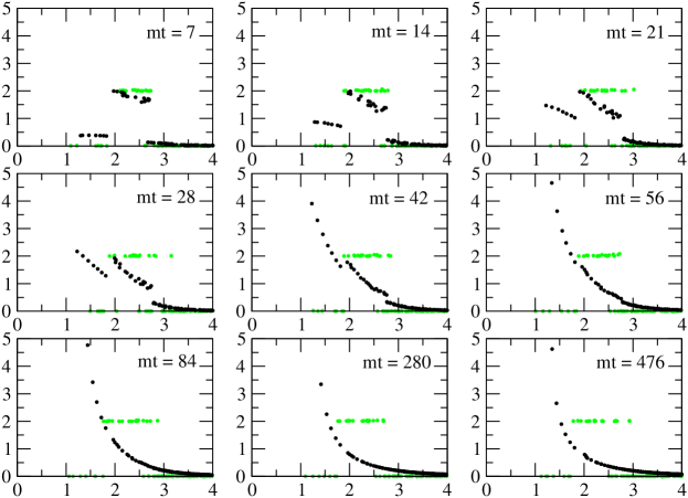
Figure 2: Evolution in time of the occupation numbers $n_{\mathbf{k}}$ vs. $\omega_{\mathbf{k}}$, for the T1 initial condition. We display the results of the “basketball” (black dots) and the Hartree approximation (green/grey dots).

In Fig. 2, we show the evolution of $n_{\mathbf{k}}$ versus $\omega_{\mathbf{k}}$, starting from the T1 initial condition. The Hartree approximation (black) is compared with the “basketball” approximation (green/grey). In the former case, there is no equilibration. For the “basketball” case, we observe that the energy in the excited modes is distributed via scattering. As we shall see this leads eventually to a thermal distribution.

In Fig. 3 we follow the evolution of the dispersion relation with the same initial condition, again comparing Hartree to “basketball”. Notice the oscillating pattern early on in both cases. In the “basketball” approximation the modes eventually relax to a perfect straight line. It turns out that at the couplings and energies used here, the coefficient $c^{2}(t)$ is equal to 1 up to well within one percent. We will therefore assume it to be 1 in the following. Although we do not show it here, we found that larger coupling and large energy density results in a faster evolution towards this quasi-particle state.

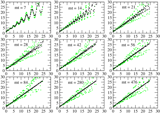
Figure 3: Time evolution of the dispersion relation ($\omega_{\mathbf{k}}^{2}$ vs. ${\mathbf{k}}^{2}$) in the symmetric phase, starting from the T1 initial conditions, in the “basketball” ( black dots) and Hartree approximations (green/grey dots).

Judging by eye, Figs. 2 and 3 suggest that already at times $mt=56$ to $84$, the system behaves as aproximately thermal, for T1 initial conditions. Still, this is presumably much later than a pre-thermalization time based on the the equation of state, as studied in Berges:2004ce . However, it does not mean that the memory of the initial conditions in the particle distribution is already lost by times $mt\gtrsim 84$.

It was remarked already in the studies in 1+1 Berges:2000ur and 2+1 dimensions Juchem:2003bi that the final state depends only on the energy density (at a given coupling). Indeed, it was found that the limit distribution function $n_{\mathbf{k}}$ corresponds to a Bose-Einstein, characterized by just one parameter, the temperature. Fig. 4 shows the evolution of individual modes when starting from the T1, T2 and T3 initial conditions, which have the same energy density. For T1 and T2 we see that the modes approach a common final value. It seems reasonable to call this stage kinetic equilibration, as the kinetic energy is redistributed over the modes to reach a Bose-Einstein distribution. However, as we will see below, the total number of particles is not adjusting as fast and it still remembers the initial state by the time kinetic equilibration is completed.

As mentioned before, the initial condition T3 has not only a different initial spectrum, but also a different total number of particles. It also reaches kinetic equilibration, but with a different kinetically equilibrated state.

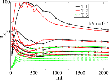
Figure 4: Evolution of individual modes for a T1 , T2 and T3 initial condition with same energy density.

At intermediate times ($mt\approx 1000$) kinetic equilibration has taken place, and we can compare the distribution functions and dispersion relations, Fig. 5. T1 and T2 have equilibrated to almost identical Bose-Einstein distribution functions, parametrized by an effective mass, an effective temperature and an effective chemical potential. T3 has reached a different Bose-Einstein with a different temperature and chemical potential, and a slightly different effective mass. We have included a number of thermal initial conditions for comparison. By construction, these have no initial chemical potential and remain so to a very good approximation.

Whereas kinetic equilibration can be the result of simple $2\leftrightarrow 2$ scattering, chemical equilibration, which changes the total particle number, happens through $1\leftrightarrow 3$, $2\leftrightarrow 4$ and higher order processes. These are included due to the resummations performed by the $\Phi$-derivable approximation into the “sunset” self-energy diagram. Approaches that only take into account on-shell scattering, such as the Boltzmann equation with only binary collisions $2\leftrightarrow 2$, cannot account for chemical equilibration. What we see is that kinetic equilibration including memory loss happens on a time scale of about $500-1000/m$, whereas chemical equilibration is a much slower process. Effectively, there is a chemical potential in the initial stages, causing initial conditions with different $N_{\rm tot}$ to relax to different intermediate kinetically equilibrated states.

      

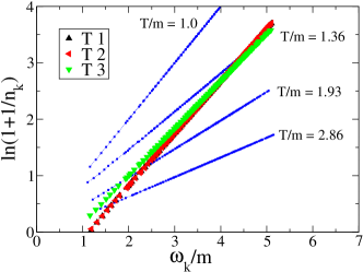
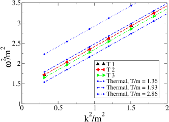
Figure 5: Left: occupation numbers $\ln(1+1/n_{\mathbf{k}})$ at intermediate times $mt=1000$ for initial T1, T2 and T3 and a set of thermal initial states. Right: The dispersion relation for the same cases. The intercepts give the effective masses squared.

      

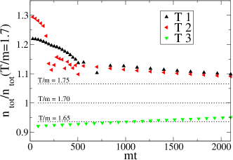
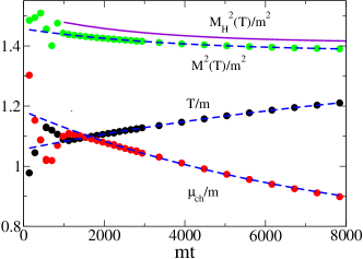
Figure 6: Left: Total particle number density $n_{\rm tot}$ versus time for the initial conditions T1, T2 and T3. The dotted lines are $n_{\rm tot}$ for Bose-Einstein distributions at different temperatures. Right: Evolution of the effective mass (squared), temperature and chemical potential for late times starting from the T1 initial condition, with exponential fits (dashed lines). The Hartree estimate for the mass, (31), and the solution of the gap equation (60), are also shown.

We illustrate this point in Fig. 6, left-hand plot, where we show the evolution $N_{\rm tot}$ for the initial conditions T1-T3. For comparison, we also include the $N_{\rm tot}$ of Bose-Einstein distributions at various temperatures. In the right-hand plot we follow the evolution of the effective mass, temperature and chemical potential for the T1 case. The time evolution can be well reproduced by exponential fits of the form $a_{i}+b_{i}\exp{(-\gamma_{i}t)}$ (the dashed lines in the plot), suggesting an asymptotic temperature of around $T/m=1.36$. Also, within a factor of two, fits to the three quantities all suggest an equilibration time of around $\gamma_{i}^{-1}\simeq 10^{4}/m$. Chemical equilibration is a full order of magnitude slower than kinetic equilibration in this system. Comparing with the study in Juchem:2003bi , it appears that chemical equilibration is much slower in 3+1 than in 2+1 dimensions. The fit to the chemical potential is not as good as to the effective temperature or mass, and it also predicts a non-zero asymptotic chemical potential ($\mu/m=0.7$). This is consistent with our above-mentioned interpretation that the system is in a prethermalized stage Berges:2004ce for which an exponential extrapolation of the evolution of $T$ and $\mu$ does not necessarily yield the actual asymptotic values.

As an aside we compare the observed mass with an estimate that results from the Hartree approximation. At a given time $t$, the finite gap equation for the Hartree effective mass reads

$$M_{\mbox{\scriptsize H}}^{2}(t)=m^{2}+\Sigma^{{\mbox{\scriptsize l}}}(t)-\delta m^{2}=m^{2}+\frac{\lambda}{2}\int\frac{d^{3}k}{(2\pi)^{3}}F_{\mathbf{k}}(t,t)-\delta m^{2}.$$ (57)

The mass counterterm $\delta m^{2}$ is given by the vacuum part of the “leaf” self-energy diagram, as described previously. For the correlator $F(t,t)$ in Eq. (57) we take the same form as a free quasiparticle gas in equilibrium, i.e.

$$F_{\mathbf{k}}(t,t)=\frac{1}{\omega_{\mathbf{k}}(t)}\left[n_{\mathbf{k}}(t)+\frac{1}{2}\right].$$ (58)

Here $n_{\mathbf{k}}(t)$ is a Bose-Einstein distribution function with the temperature and chemical potential obtained from the simulations at time $t$, and $\omega_{\mathbf{k}}(t)$ is here defined in terms of the effective mass as $\omega_{\mathbf{k}}(t)=\sqrt{\smash[b]{\mathbf{k}^{2}+M_{\mbox{\scriptsize H}}(t)^{2}}}$. The result for the Hartree effective mass $M_{\mbox{\scriptsize H}}$ is then determined by the self-consistent gap equation

$$M_{\mbox{\scriptsize H}}^{2}(t;T,\mu)=m^{2}+\frac{\lambda}{2}\int\frac{d^{3}k}{(2\pi)^{3}}\frac{n_{\mathbf{k}}(t;T,\mu)}{\omega_{\mathbf{k}}(t)}=m^{2}+\frac{\lambda T^{2}}{4\pi^{2}}\int_{M_{\mbox{\tiny H}}/T}^{\infty}dx\frac{\sqrt{x^{2}-\frac{M_{\mbox{\tiny H}}^{2}}{T^{2}}}}{e^{\left(x-\frac{\mu}{T}\right)}-1}.$$ (59)

To compare with the numerical result we use the lattice analog of the gap equation (59), i.e.

$$M_{\mbox{\scriptsize H}}^{2}(t;T,\mu)=m^{2}+\frac{\lambda}{2}\frac{1}{(Na)^{3}}\sum_{\mathbf{k}}\frac{n_{\mathbf{k}}(t;T,\mu)}{\omega_{\mathbf{k}}(t)}.$$ (60)

For the case of the evolution starting from the T1 initial condition, the lattice Hartree mass is shown in Fig. 6. We see that it is slightly higher than the effective mass obtained in the simulation with the “basketball” approximation. At least in this case, the contribution from the “sunset” diagram to the mass appears to be small relative to the Hartree case.

IV.5 Symmetric phase: Damping and the spectral function

IV.5.1 Mean field damping

We now consider a situation already in (or close to) thermal equilibrium, where the mean field is slightly displaced from its equilibrium value $\phi=0$. This allows us to study the response of the system to small perturbations. In this case, the mean field evolution can be studied by linearizing the equation of motion (32) around the equilibrium value. For homogeneous fields this leads to

$$\overset{..}{\phi}(t)+M^{2}(T,t)\phi(t)+\int_{0}^{t}dt^{\prime}\,\tilde{\Sigma}^{\rho}_{\mathbf{0}}(t,t^{\prime})\,\phi(t^{\prime})=0.$$ (61)

with $\tilde{\Sigma}^{\rho}_{\mathbf{0}}(t,t^{\prime})$ the zero momentum mode of the “sunset” self-energy and $M(T,t)$ given by (31). Close enough to equilibrium we may assume time translation invariance, such that $\tilde{\Sigma}^{\rho}_{\mathbf{0}}(t,t^{\prime})$ depends only on $t-t^{\prime}$ and $M(T,t)$ is constant. The equation (61) can then be solved by a Laplace transform in the time coordinate Boyanovsky:1996xx . Taking as initial conditions for the mean field $\phi(0)=\phi_{i}$ and $\overset{.}{\phi}(0)=0$, the solution to the linearized equation of motion (61) can be written as Boyanovsky:1995me ; Boyanovsky:1996xx

$$\phi(t)=\frac{2\phi_{i}}{\pi}\int_{0}^{\infty}d\omega\frac{\omega\,\mbox{Im}\tilde{\Sigma}^{R}_{\mathbf{0}}(\omega)\,\cos(\omega t)}{\left[\omega^{2}-M^{2}-\mbox{Re}\tilde{\Sigma}^{R}_{\mathbf{0}}(\omega)\right]^{2}+\mbox{Im}\tilde{\Sigma}^{R}_{\mathbf{0}}(\omega)^{2}},$$ (62)

where $\mbox{Re}\tilde{\Sigma}^{R}$ and $\mbox{Im}\tilde{\Sigma}^{R}$ correspond respectively to the real and imaginary part of the retarded self-energy, given by $\tilde{\Sigma}^{R}(x,y)=\Theta(x_{0}-y_{0})\tilde{\Sigma}^{\rho}(x,y)$. For weak coupling there is a narrow resonance at $\omega=M_{\mbox{\scriptsize eff}}$, with $M_{\mbox{\scriptsize eff}}^{2}\equiv M^{2}+\mbox{Re}\tilde{\Sigma}^{R}_{\mathbf{0}}(\omega)$. To a good approximation, one finds that for short times the evolution is given by Boyanovsky:1995em

$$\phi(t)\approx\phi_{i}Z\,e^{-\gamma t}\cos\left(M_{\mbox{\scriptsize eff}}t-\alpha\right),$$ (63)

with

$$Z =\bigg{[}1-\frac{\partial\mbox{Re}\tilde{\Sigma}^{R}_{\mathbf{0}}(M_{\mbox{\scriptsize eff}})}{\partial M^{2}_{\mbox{\scriptsize eff}}}\bigg{]}^{-1},$$ (64)

$$\alpha =\frac{\partial\mbox{Im}\tilde{\Sigma}^{R}_{\mathbf{0}}(M_{\mbox{\scriptsize eff}})}{\partial M^{2}_{\mbox{\scriptsize eff}}},$$ (65)

$$\gamma =Z\frac{\mbox{Im}\tilde{\Sigma}^{R}_{\mathbf{0}}(M_{\mbox{\scriptsize eff}})}{M_{\mbox{\scriptsize eff}}}.$$ (66)

The parameter $\gamma$ corresponds to the on-shell damping rate. For weak enough couplings one can approximate $Z\approx 1$ and $M_{\mbox{\scriptsize eff}}=M$ for the calculation of $\gamma$. From (66) we see that the damping rate is determined by the imaginary part of $\tilde{\Sigma}^{R}$, which corresponds to the “sunset” self-energy diagram. In the context of perturbation theory, $\mbox{Im}\,\tilde{\Sigma}^{R}$ can be calculated analytically and the damping rate is found to be Wang:1996qf

$$\gamma(M)=\frac{\lambda^{2}T^{2}}{128\pi^{3}M}\,\mbox{Li}_{2}(e^{-M/T})$$ (67)

where $\mbox{Li}_{2}(z)$ is the second polylogarithmic function, defined by Spence’s integral

$$\mbox{Li}_{2}(z)=-\int_{0}^{z}dw\frac{\ln\left({1-w}\right)}{w}.$$ (68)

For temperatures $T\gg m$, the damping rate follows from the expression of the high-temperature screening mass Arnold:1992rz

$$M^{2}=m^{2}+\frac{\lambda T^{2}}{24}-\frac{\lambda}{8\pi}M\,T+\mathcal{O}\left(\lambda M\,\mbox{ln}\frac{M^{2}}{T^{2}}\right).$$ (69)

In the limit of very weak coupling and high temperature one obtains for the damping rate the compact result Jeon:1992kk ; Wang:1996qf

$$\gamma\Big{|}_{T\gg m,\,\lambda\ll 1}=\frac{\lambda^{2}T^{2}}{768\pi M}.$$ (70)

In the numerical simulations the mean field is initially displaced to the value $\phi_{i}/m=0.142$. For such a small perturbation, the mean field is expected to perform a damped oscillation of the type (63). We fit the evolution of the mean field with Eq. (63), which allows us to extract the effective mass $M_{\mbox{\scriptsize eff}}$ and the damping rate $\gamma$. These will depend on the strength of the coupling and the temperature. The behavior of the mean field is studied in a thermal bath at temperatures $T_{\mbox{\scriptsize in}}/m=0,1.43,2.86$ for both the two-loop and “basketball” approximations. For the “basketball” case, the mean field evolution is shown in Fig. 7.

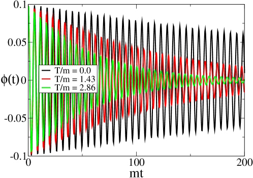
Figure 7: Time evolution $\phi(t)$ of the initially displaced mean field $\phi_{i}=0.142$ for the cases $T_{\mbox{\scriptsize in}}/m=0,1.43,2.86$, in the “basketball” approximation.

As mentioned earlier, the damping of the mean field is present in both the two-loop and “basketball” approximations. The difference between the two cases lies in the fact that the correlators $F$ and $\rho$ evolve quite differently. For the two-loop case, the equations of motion for $F$ and $\rho$ contain almost no damping, since the only potential contribution to damping is in the “eye” diagram, which is proportional to $\phi^{2}$, and thus tiny for $\phi\approx 0$. For the “basketball” case, however, the equations of motion for $F$ and $\rho$ contain damping through the “sunset” diagram. The differences in the evolution of the correlators for the two-loop and the “basketball” approximations enters as a higher-order effect in the evolution of the mean field. In particular, this may lead to different effective masses and mean field damping rates. We show these differences for various temperatures in Fig. 8, where the results for the two-loop (squares) and “basketball” (large dots) are plotted.

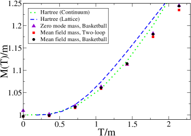
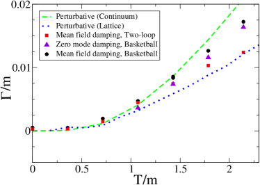
Figure 8: Left: Effective masses from the analysis of the evolution of the mean field (in the two-loop and “basketball” aproximations) and spectral function zero-mode (“basketball” case). Hartree estimates, both in the continuum (dotted line) and on the lattice (dashed line), are also shown. Right: Damping rates.

For comparison we evaluated the perturbative result (67), using the Hartree mass (59) for $M$. To see the finite-volume and discretization effects we also did the analytical computation on a spatial lattice. The Hartree mass is in this case given by (60). In finite volume, the discreteness of the momenta leads to complications in the calculation of the damping rate, which we dealt with along the lines presented in Salle:2000jf . The perturbative results for the mass and damping rate are also presented in Fig. 8. As we can see from the mass plot (left), the correction to the mass coming from the “basketball” approximation is small relative to the Hartree case. In the damping plot (right) we observe that the damping rate obtained from the numerical analysis of both approximations is substantially larger (about 20-40%) than the perturbative result (on the lattice). The continuum and the lattice perturbative results begin to differ around $T/m\gtrsim 1$ due to cut-off effects.

IV.5.2 Propagator damping and spectral function

Damping in the propagator can be elegantly phrased in terms of the spectral function $\rho_{\bf k}(t,t^{\prime})$. In a situation close to thermal equilibrium we expect it to be time translation invariant and in a narrow-width approximation be given by

$$\rho_{\bf k}(t,t^{\prime})=\frac{1}{\omega_{\mathbf{k}}}e^{-\gamma_{\bf k}|t-t^{\prime}|}\sin\left[\omega_{\bf k}(t-t^{\prime})\right],$$ (71)

To study the approach to equilibrium of the spectral funcion, it is useful to perform a Wigner transformation in terms of the mean time $\mathcal{T}=(t+t^{\prime})/2$ and relative time $\tau=t-t^{\prime}$. This can be written as

$$\rho_{\bf k}(\omega,\mathcal{T})=2i\int_{0}^{2\mathcal{T}}d\tau\sin(\omega\tau)\rho_{\bf k}(\mathcal{T}+\tau/2,\mathcal{T}-\tau/2).$$ (72)

Since we are solving the equations of motion in a finite time and keep information only as far back as the memory kernel, we have a cut-off in the integral of (72) as

$$\rho_{\bf k}(\omega,\mathcal{T})\approx\rho_{\bf k}(\omega,\mathcal{T};t_{\mbox{\scriptsize cut}})=2i\int_{0}^{t_{\mbox{\scriptsize cut}}}d\tau\sin(\omega\tau)\rho_{\bf k}(\mathcal{T}+\tau/2,\mathcal{T}-\tau/2).$$ (73)

If the system is sufficiently close to equilibrium, time translation invariance should be a good approximation, $\rho_{\bf k}(t,t^{\prime})\approx\rho_{\bf k}(t-t^{\prime})$, and

$$\rho_{\bf k}(\omega,\mathcal{T};t_{\mbox{\scriptsize cut}})\approx 2i\int_{0}^{t_{\mbox{\scriptsize cut}}}d\tau\,\sin{(\omega\tau)}\,\rho_{\bf k}(\mathcal{T},\mathcal{T}-\tau).$$ (74)

With this approximation the integrand in (74) runs from $\rho_{\mathbf{k}}(\mathcal{T},\mathcal{T})$ to $\rho_{\mathbf{k}}(\mathcal{T},\mathcal{T}-t_{\mbox{\scriptsize cut}})$, which is convenient for numerical purposes. In the following we shall make use of this approximate Wigner transform.

The approximation (74) is valid provided $\mathcal{T}$ is large enough so that the system is close to thermal equilibrium. In that case $\rho_{\bf k}(\omega_{\bf k},\mathcal{T})$ should be well approximated by a Breit-Wigner form

$$\rho_{\bf k}(\omega,\mathcal{T})\approx\frac{4\omega(\gamma_{\bf k}/2)}{(\omega^{2}-\omega_{\bf k}^{2})^{2}+\omega^{2}(\gamma_{\bf k}/2)^{2}}.$$ (75)

The evolution of the spectral function $\rho_{\bf k}(t,t^{\prime})$ starting from a thermal background at $T/m=2.86$ and $\lambda=6$ is shown for two different kernel lengths, $mt_{\rm cut}=28$ (green/grey) and $mt_{\rm cut}=84$ (black), in Fig. 9 (left). Overlaid, although barely discernible, a fit of the form (71). As can be seen, the fit is excellent and it is the same fit for the two kernel lengths. In Fig. 9 (right) we show the result of the approximate Wigner transforms for the spectral function of the spatial zero mode at $m\mathcal{T}=200$ and with two different kernel lengths. For the long kernel case, one can nicely fit a Breit-Wigner form, which gives the same damping rates and masses as in the fit of the left-hand plot. For the short kernel case, the Breit-Wigner fit is not so accurate. In the following analysis, we extract the damping rates and masses from fits directly to the time-representation of the spectral function $\rho_{\mathbf{k}}(t,t^{\prime})$, with kernel length $mt_{\rm cut}=28$.

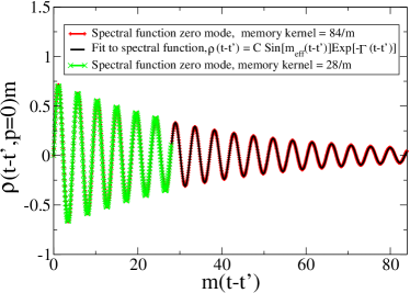
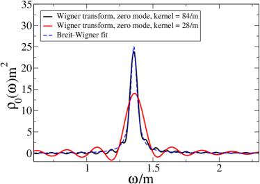
Figure 9: Left: The evolution of the spectral function $\rho_{\mathbf{0}}(t,t^{\prime})$ starting from a thermal initial condition with $T/m=2.86$ and with coupling $\lambda=6$. The result with a short and a long kernel is plotted. Overlaid a fit to the form (71). Right: The approximate Wigner transform $\rho_{\mathbf{0}}(\omega)$ at time $m\mathcal{T}=200$. A Breit-Wigner fit to the Wigner transform with kernel $84/m$ is included (dashed line).

Fig. 8 shows the dependence on temperature of the effective mass (left) and damping rate (right) from fits of the form (71) for the spectral function zero-mode $\rho_{\mathbf{0}}(t,t^{\prime})$, together with the fits (63) for the mean field discussed earlier. For $\rho_{\mathbf{0}}(t,t^{\prime})$, we show only the results for the case of the “basketball” approximation, since, for the values of the mean field considered here, it is practically zero in the two-loop approximation. The spectral-function zero-mode mass and damping rate (plotted with triangles) closely follow the values for the mean field.

IV.6 Broken phase: equilibration

A similar analysis can be carried out in the broken phase, where there is a non-zero mean field present. In this case we can use both the two-loop and “basketball” approximations to study the damping of the correlators. From the point of view of perturbation theory, there is no damping in the two-loop approximation, for which only the perturbative “leaf” and the “eye” diagrams contribute to the self-energy, and their imaginary parts vanish on-shell (see also appendix B). Our task will be to study the damping in the two-loop approximation from the $\Phi$-derived equations of motion. These formally take into account the contributions from all orders in perturbation theory that result from any iterated insertion of the “leaf” and “eye” diagrams into the self-energy. These diagrams contain off-shell scattering effects that can, in principle, lead to a total non-zero on-shell imaginary part for the self-energy, thus providing damping. For the case of the “basketball” approximation, the “sunset” diagram enters in the self-energy (13), which contributes to damping even in perturbation theory Jeon:1992kk ; Wang:1996qf . The solution of the $\Phi$-derived equations of motion leads to additional contributions from higher orders compared to perturbation theory, and thus one expects to find a larger damping and faster equilibration.

Approximations based on truncations of the loop expansion of the 2PI effective action suffer from instabilities which make it impossible to treat very large couplings and very large energy densities or particle numbers. In this sense, the $\Phi$-derived equations of motion can be thought of as resummed perturbative, useful in the domain of weak coupling and small fields. In the symmetric-phase simulations described previously, $\lambda=6$ is in the upper end of what stays stable in our experience, whereas we can use temperatures (or energy densities corresponding to temperatures) up to $T/m=6$ or even higher. In the broken phase, the instabilities turn out to be even more constraining. In particular, we will need to use a smaller coupling ($\lambda=1$) and temperatures below $T/m=2$. As we have seen, the latter is not much of a restriction since it still covers the region where cut-off effects are small. However, it implies that equilibration and damping takes much longer (the damping times scale roughly as $\lambda^{2}T^{2}$ for the sunset diagram). In particular we need to use a longer time kernel (we use $mt_{\rm cut}=84$) and we will not be able to track the evolution far enough to see chemical equilibration. We shall content ourselves with establishing kinetic equilibration and studying the damping of the mean field and the modes of the spectral function. We have no doubt that chemical equilibration will take place as well. In particular, we will see that total particle number is not conserved.

The mean field is taken initially to be at the tree-level value $\phi(t=0)=v_{\mbox{\scriptsize tree}}$. This is not the self-consistent finite temperature solution of the truncated equations of motion, but a bit displaced from it. Due to this initial displacement, the mean field will oscillate and damp to its equilibrium value. For the propagators we will use thermal initial conditions, as well as top-hat 1 (T1). Notice that the input mass is the broken phase zero temperature mass $\sqrt{2}m$ rather than the symmetric phase one. All results are still in units of $m$.

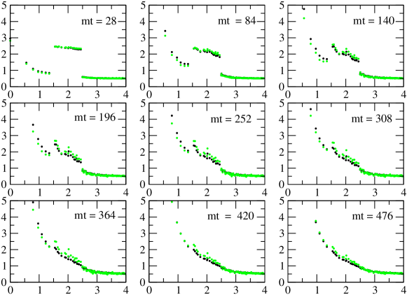
Figure 10: Evolution of the occupation numbers ($n_{\bf k}$ vs. $\omega_{\bf k}/m$), starting from the T1 initial condition, in the broken phase ($\lambda=1$) and in the two-loop (green/grey) and “basketball” (black) approximations, respectively.

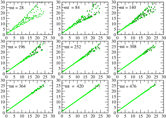
Figure 11: Evolution of the dispersion relation ($\omega_{\bf k}^{2}/m^{2}$ vs. $k^{2}/m^{2}$), with the T1 initial condition, in the two-loop (green/grey) and basketball (black) approximations, respectively.

The evolution of the occupation numbers and the dispersion relation for both the two-loop and “basketball” approximations are shown in Fig. 10 and Fig. 11. Both cases show that (kinetic) equilibration is taking place. In the “basketball” case, equilibration is slightly faster. Interestingly, the off-shell scattering effects taken into account by the 2PI effective action with only the eye diagram lead to an equilibration almost as fast as in the “basketball” case. Chemical equilibration happens on much longer time scales, and although we found that the total particle number does change in time (Fig. 12, left), the reach of our simulations was insufficient to estimate the asymptotic temperature. At our latest time of $mt=1000$, the distribution is consistent with a Bose-Einstein with $T/m=1.24$ and $\mu/m=1.12$ (Fig. 12, right).

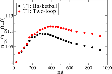
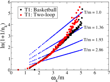
Figure 12: Left: The total particle number density $n_{\mbox{\scriptsize tot}}(t)$ for the two truncations, normalized to the initial value. Right: Particle distributions at the latest time $mt=1000$, for T1 and thermal initial conditions.

IV.7 Broken phase: Mean field damping and the spectral function

For weak coupling we expect the position of the equilibrium mean field expectation value $v$ to be close to the initial value $\phi(0)=v_{\mbox{\scriptsize tree}}$. In the case of thermal initial conditions, the initial mean field displacement corresponds to a small perturbation. As in the symmetric phase case, one can study the evolution of the mean field by linearizing the equation of motion around the equilibrium value. We write $\phi(t)=v+\sigma(t)$, where $\sigma(t)$ is the deviation. The linearized equation of motion for $\sigma$ is then

$$\overset{..}{\sigma}(t)+M^{2}(T,t)\sigma(t)+\int_{0}^{t}dt^{\prime}\,\tilde{\Sigma}_{\mathbf{0}}^{\rho}(t,t^{\prime})\sigma(t^{\prime})=0.$$ (76)

The vacuum expectation value $v$ is the solution of

$$M^{2}(T,t)v-\frac{\lambda}{3}v^{3}+\int_{0}^{t}dt^{\prime}\,\tilde{\Sigma}_{\mathbf{0}}^{\rho}(t,t^{\prime})v=0.$$ (77)

For weak coupling

$$v\approx\sqrt{\frac{3M^{2}(T)}{\lambda}}.$$ (78)

In Eqns.(76-78), $M(T,t)$ corresponds to the finite temperature Hartree effective mass in the broken phase, given by

$$M^{2}(T,t)=-m^{2}+\frac{\lambda}{2}v^{2}+\frac{\lambda}{2}\int\frac{d^{3}\;k}{(2\pi)^{3}}F_{\mathbf{k}}(t,t)-\delta m^{2}.$$ (79)

The analysis of the evolution of $\sigma$ proceeds as in the case of the symmetric phase. For weak enough coupling the mean field damping rate is approximately given by the perturbative estimate (67).

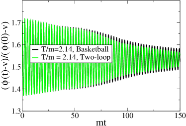
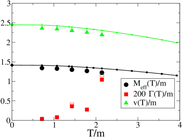
Figure 13: Left: Evolution of the mean field in the broken phase in a thermal background at $T/m=2.14$, in the two-loop and “basketball” approximations. Right: Effective masses, vacuum expectation values and damping rates from fits of the form (63) for both the two-loop (empty symbols) and “basketball” (filled symbols) approximations. The lines represent the Hartree approximation.

Fig. 13 (left) shows the mean field evolution at $T/m=2.14$, in the two-loop and “basketball” approximations, respectively. In both cases, the mean field performs a damped oscillation, from which we can extract an effective mass and mean field expectation value. As we can see, the damping does not follow a simple exponential form, and curiously, the two-loop data appear to indicate faster damping than the basketball data. Still, we shall use an exponential fit as a rough estimate of the damping rate. The temperature dependence of these frequencies and damping rates, in addition to the field expectation values, is shown in Fig. 13 (right) for the two-loop (open symbols) and “basketball” (filled symbols) approximations. The masses and field expectation values are indistinguishable for the two truncations. They are slightly off the respective Hartree estimates (77) and (79) (full lines), indicating as in the previous section that the contribution of the “sunset” diagram in the “basketball” approximation is small relatively to the Hartree case. The damping rates in the two approximations are consistent with each other.

Similarly, we observed damping in the evolution of the spectral function $\rho_{\bf k}(t,t^{\prime})$ in both approximations. This damping is small and not well approximated by an exponential form. We performed the Wigner transformation as specified in Eq. (74), see Fig. 14 to the data of the late time evolution starting from the T1 initial condition. The value of the cut-off $t_{\mbox{\scriptsize cut}}=84\,m^{-1}$ produces some noise, but for the “basketball” approximation (full lines) there is clearly a well determined peak with a finite width at all times, which can be fit with a Breit-Wigner form (dashed lines). In the basketball approximation, the form of the Wigner transform does not change much in time, which indicates that the system is relatively close to equilibrium. However, the results are different for the approximate Wigner transforms in the two-loop approximation (dotted lines). In this case the transformed spectral function changes significantly in time from thin peaks early on to less clear maxima at later times, still localized around the peaks, see Fig 14 (right). We do not fully understand the reason for this discrepancy; it could be, that the cut-off time $t_{\mbox{\scriptsize cut}}=84\,m^{-1}$ in our implementation of the Wigner transform is too short in case of the two-loop approximation. On the other hand, the large $\mathcal{T}$-dependence of the spectral function indicates that the system may not be sufficiently close to equilibrium in the two-loop approximation, in which case the use of the approximate Wigner transform (74) is questionable. The approximation itself appears to work reasonably well, as shown in Figs. 12 and 13.

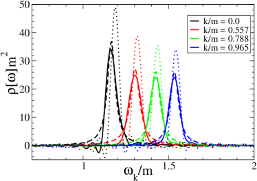
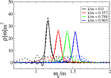
Figure 14: Wigner transforms of the spectral function for the four lowest modes, starting from a T1 initial condition, at two times (left plot, $m\mathcal{T}=252$ and right plot, $m\mathcal{T}=1000$) for the “basketball” (full lines) and two-loop (dotted lines) approximations. The weak $\mathcal{T}$-dependence of the former shows that the system is close to equilibrium. Indeed, Breit-Wigner fits work nicely (dashed lines). The strong $\mathcal{T}$-dependence in the two-loop case suggests that the system is not yet sufficiently close to equilibrium.

V Conclusions

We have studied equilibration in $\varphi^{4}$ theory in 3+1 dimensions for a variety of initial conditions, both in the symmetric and broken phase. Two different $\Phi$-derivable approximations including scattering effects have been used: two-loop and “basketball”, the latter corresponding to a truncation of the 2PI effective action at $\mathcal{O}(\lambda^{2})$. In the symmetric phase the two-loop and the “basketball” approximations differ in that the first includes damping into the evolution of the mean field only, whereas in the second it is also present in the equation of motion for the 2-point functions. In the broken phase both approximations include scattering effects into the 2-point functions and thus can lead to equilibration.

From the numerical study of the evolution of the occupation numbers we were able to establish that in the symmetric phase both kinetic and chemical equilibration is taking place, the latter at a substantially slower rate.

By analyzing various initial conditions we found that, after kinetic equilibration, the occupation numbers at intermediate times are given by a Bose-Einstein distribution with an effective chemical potential. This is similar to what was found in previous studies in 2+1 dimensions Juchem:2003bi . Given the same total energy, we found the intermediate effective chemical potential to be generally non-zero, with its size related to the initial total particle numbers, as may be expected. Eventually, one would expect the limit distribution to depend only on the energy density of the system, and close to a Bose-Einstein with zero chemical potential Berges:2000ur ; Juchem:2003bi . Comparing to the studies in 2+1 dimensions Juchem:2003bi , our numerical analysis indicates that the subsequent chemical equilibration is much slower in 3+1 dimensions.

We were also able to extract effective masses and damping rates from the analysis of the evolution of the mean field and the spectral function. The contributions to the mass from the two-loop and the “basketball” approximations seem to be small comparing to the Hartree case. In the symmetric phase, the results for the damping rate are about a 20-40$\%$ higher than the perturbative estimates. This indicates that the scattering effects associated with the resummations encoded in the $\Phi$-derivable approximation are substantial. Finally, we checked that the damping rate obtained from the mean field coincides with the one from the spectral function zero-mode.

In the broken phase we found that both the two-loop and the “basketball” approximation lead to equilibration. Surprisingly, the equilibration seems to be just a bit slower in the two-loop case. This is particularly remarkable, since, in perturbation theory, the two-loop approximation does not have on-shell damping. Indeed, in that case only the perturbative “leaf” and “eye” self-energy diagrams contribute, and their imaginary parts vanish on-shell (see appendix B). The fact that the two-loop approximation in $\varphi^{4}$ theory equilibrates so fast might be relevant to pure gauge theories, where the lowest order $\Phi$-derivable approximation (at $\mathcal{O}(g^{2})$) considers the same diagrams.

On a practical note, we found that the loop expansion suffers from restrictions reminiscent of perturbative expansions, in that large couplings and/or large field occupation numbers trigger instabilities when solving the equations of motion. This has to our knowledge not been reported for simulations in 1+1 and 2+1 dimensions, although we have found them in those cases as well. In addition to the instabilities, issues such as CPU time and computer memory necessary for dealing with the memory integrals are significant restrictions, especially when studying late time thermalization. Expansions in $1/N$ with $N$ the number of fields have been shown to be more stable and able to deal with non-perturbatively large occupation numbers at large coupling Berges:2001fi ; Berges:2002cz ; Mihaila:2003mh ; Arrizabalaga:2004iw . In such cases care should be taken to ensure that the expansion is controlled by using a sufficiently large value of $N$ Aarts:2001yn .

Appendix A: Energy-momentum tensor in $\Phi$-derivable approximations

The energy-momentum tensor for a given truncation of the 2PI effective action can be determined through Noether’s procedure, i.e. by identifying the current term resulting from the space-time dependent translations $x^{\mu}\rightarrow x^{\mu}+\epsilon^{\mu}(x)$. A convenient way to find the Noether current is to pertorm an infinitesimal translation that vanishes on the space-time boundary. The translation $x^{\mu}\rightarrow x^{\mu}+\epsilon^{\mu}(x)$ can be viewed as a transformation of the relevant variables, which in the case of the 2PI effective action are the mean field $\phi(x)$ and the connected 2-point function $G(x,y)$. This transformation is given by

$$\phi(x) \longrightarrow\phi^{\prime}(x)\equiv\phi(x+\epsilon(x))=\phi(x)+\epsilon^{\lambda}(x)\partial^{x}_{\lambda}\phi(x),$$ (80)

$$G(x,y) \longrightarrow G^{\prime}(x,y)\equiv G(x+\epsilon(x),y+\epsilon(y))=G(x,y)+\epsilon^{\lambda}(x)\partial^{x}_{\lambda}G(x,y)+\epsilon^{\lambda}(y)\partial^{y}_{\lambda}G(x,y),$$ (81)

where the variables that the partial derivatives act on are indicated with a superscript. Under these transformations the variation of the 2PI effective action $\Gamma[\phi,G]$ can be formally written as

$$\delta\Gamma[\phi,G]=\int_{x}\;T^{\mu\nu}(x)\partial_{\mu}\epsilon_{\nu}(x),$$ (82)

where $\int_{x}\equiv\int d^{4}x$. The quantity $T^{\mu\nu}$ defines a conserved Noether current, which is identified as the energy-momentum tensor. To see that it is indeed conserved, notice that when the $\Phi$-derived equations of motion for $\phi$ and $G$ are satisfied. This applies, in particular, to the transformations (80) and (81), and hence $\delta\Gamma[\phi,G]=0$. Taking (82) and making a partial integration one obtains

$$\delta\Gamma[\phi,G]=-\int_{x}\;\epsilon_{\nu}(x)\,\partial_{\mu}T^{\mu\nu}(x)=0.$$ (83)

Since $\epsilon_{\nu}(x)$ can be taken arbitrary, the energy-momentum tensor is conserved, i.e. $\partial_{\mu}T^{\mu\nu}(x)=0$.
Below we give the explicit form of the energy-momentum tensor $T^{\mu\nu}$ for any $\Phi$-derivable approximation by applying the transformations (80-81) and using the definition (82). We study independently the contributions coming from the four terms in the action (2):

• The first term in Eq. (2) is given by $S[\phi]$ and leads to the usual form of the energy-momentum tensor for the mean field $\phi$, namely

  $$T_{1}^{\mu\nu}(x)=\partial^{\mu}\phi(x)\partial^{\nu}\phi(x)-g^{\mu\nu}\left[\frac{1}{2}\partial_{\lambda}\phi(x)\partial^{\lambda}\phi(x)-\frac{1}{2}m^{2}\phi(x)^{2}-\frac{\lambda}{4!}\phi(x)^{4}\right].$$ (84)

• The second term appearing in Eq. (2) does not contribute to the energy-momentum tensor. Indeed, applying the transformations (81) leads to

  $$\delta\left[{\rm Tr}\ln G\right]={\rm Tr}G^{-1}\delta G\\ =\int_{x}\int_{y}G^{-1}(y,x)\left[\epsilon^{\lambda}(x)\partial_{\lambda}G(x,y)+(x\leftrightarrow y)\right]=2\int_{x}\epsilon^{\lambda}(x)\partial_{\lambda}^{x}\delta^{(4)}(x-x)=0.$$ (85)

  Hence, the corresponding contribution $T^{\mu\nu}_{2}(x)$ to the energy-momentum tensor vanishes.

• To obtain the contribution from the third term, given by $(i/2)\,\mbox{Tr}\left[G_{0}^{-1}-G^{-1}\right]G$, one proceeds similarly to what was done in i). Under the transformation (81), it becomes

  $$\delta\left[\frac{i}{2}\mbox{Tr}\left[G_{0}^{-1}-G^{-1}\right]G\right]=\\ \frac{1}{2}\int_{x}\int_{y}\left(-\partial_{\mu}^{x}\partial^{\mu}_{x}-m^{2}-\frac{\lambda}{2}\phi(x)^{2}\right)\delta^{(4)}(x-y)\left[\epsilon^{\lambda}(x)\partial_{\lambda}^{x}G(x,y)+(x\leftrightarrow y)\right]\\ -\frac{1\lambda}{2}\int_{x}\int_{y}\phi(x)\epsilon^{\lambda}(x)\partial_{\lambda}^{x}\phi(x)\delta^{(4)}(x-y)G(x,y).$$ (86)

  After some partial integrations and making use of the identity

  $$\int_{y}\partial_{x}^{\mu}\left[\delta^{(4)}(x-y)G(x,y)\right]=\int_{y}\delta^{(4)}(x-y)\left[\partial_{x}^{\mu}G(x,y)+\partial_{x}^{\mu}G(y,x)\right],$$ (87)

  one can write the above in the form given by Eq. (82), which allows to extract the contribution of this term to the energy-momentum tensor. One finds

  $$T_{3}^{\mu\nu}(x)=\int_{y}\delta^{(4)}(x-y)\left[\partial^{\mu}_{x}\partial^{\nu}_{y}-\frac{1}{2}g^{\mu\nu}\partial^{\lambda}_{x}\partial_{\lambda}^{y}+\frac{1}{2}g^{\mu\nu}m^{2}+\frac{1}{4}g^{\mu\nu}\lambda\phi(x)^{2}\right]G(x,y).$$ (88)

• For the fourth term in Eq. 2, which is given by the functional $\Phi[\phi,G]$, the transformations (80-81) give

  $$\delta\Phi[\phi,G]=\int_{x}\frac{\delta\Phi}{\delta\phi(x)}\epsilon_{\mu}(x)\partial_{x}^{\mu}\phi(x)+\int_{x}\int_{y}\frac{\delta\Phi}{\delta G(x,y)}\left[\epsilon_{\mu}(x)\partial^{\mu}_{x}G(y,x)+\epsilon_{\mu}(y)\partial^{\mu}_{y}G(y,x)\right].$$ (89)

  What we want is to write this in a form similar to (82) such that its contribution to the energy-momentum tensor can be extracted. To do this, notice that the functional $\Phi[\phi,G]$ is a scalar quantity that does not contain derivative terms. This means that, under the space-time translation $x^{\mu}\rightarrow x^{\mu}+\epsilon^{\mu}(x)$, the terms in $\Phi$ only change by the appearance of the Jacobian of the transformation at every loop integration. This Jacobian can be accommodated by a simultaneous change in a scale factor $\zeta(x)$ introduced at every integration vertex as $\lambda\rightarrow\zeta(x)\lambda$ Baym:1962sx ; Ivanov:1998nv . Thus the simultaneous variation

  $$\phi(x)\rightarrow\phi(x+\epsilon(x)),\quad G(x,y)\rightarrow G(x+\epsilon(x),y+\epsilon(y)),\quad\zeta(x)=1\rightarrow\zeta(x)=\mbox{det}\left(\delta^{\mu}_{\nu}+\partial_{\nu}^{x}\epsilon^{\mu}(x)\right)$$ (90)

  leaves the functional $\Phi$ invariant. For infinitesimal transformations, this invariance implies

  $$\int_{x}\frac{\delta\Phi}{\delta\phi(x)}\epsilon_{\mu}(x)\partial_{x}^{\mu}\phi(x)+\int_{x}\int_{y}\frac{\delta\Phi}{\delta G(x,y)}\left[\epsilon_{\mu}(x)\partial^{\mu}_{x}G(y,x)+\epsilon_{\mu}(y)\partial^{\mu}_{y}G(y,x)\right]+\int_{x}\frac{\delta\Phi}{\delta\zeta(x)}\partial_{\mu}^{x}\epsilon^{\mu}(x)=0.$$ (91)

  One can then use the identity (91) to write the variation $\delta\Phi[\phi,G]$ in a form similar to (82) as

  $$\delta\Phi[\phi,G]=-\int_{x}\frac{\delta\Phi}{\delta\zeta(x)}\Big{|}_{\zeta=1}\partial_{\mu}^{x}\epsilon^{\mu}(x).$$ (92)

  In this manner, the contribution of the functional $\Phi$ to the energy momentum tensor can be written as

  $$T^{\mu\nu}_{4}(x)=-g^{\mu\nu}\frac{\delta\Phi}{\delta\zeta(x)}\Big{|}_{\zeta=1}.$$ (93)

The total energy-momentum tensor is obtained by adding up all the contributions from i)-iv), i.e. $T^{\mu\nu}(x)=T_{1}^{\mu\nu}(x)+T_{2}^{\mu\nu}(x)+T_{3}^{\mu\nu}(x)+T_{4}^{\mu\nu}(x)$. The result can be compactly written as

$$T^{\mu\nu}(x)=\left[\partial_{x}^{\mu}\partial^{\nu}_{y}-\frac{1}{2}g^{\mu\nu}\partial_{\lambda}^{x}\partial_{y}^{\lambda}+\frac{1}{2}g^{\mu\nu}m^{2}\right]\big{(}\phi(x)\phi(y)+G(x,y)\big{)}\Big{|}_{x=y}\\ +g^{\mu\nu}\frac{1}{4!}\lambda\phi(x)^{4}+\frac{1}{4}g^{\mu\nu}\phi(x)^{2}G(x,x)-g^{\mu\nu}\frac{\delta\Phi}{\delta\zeta(x)}\Big{|}_{\zeta=1}.$$ (94)

Appendix B: Perturbative damping from the ”eye” diagram

For completeness, we include here the calculation of the imaginary part of the perturbative “eye” diagram in equilibrium in the real-time formalism, using the Schwinger-Keldysh contour. More details can be found in e.g. LeBellac . We introduce the labels $+$ or $-$ to indicate whether the time variables of any quantity live respectively on the $\mathcal{C}^{+}$ or $\mathcal{C}^{-}$ branch of the contour. In terms of the various contour components, the retarded self-energy is given by $\Sigma^{R}(x,y)=\Sigma^{++}(x,y)+\Sigma^{+-}(x,y)$. For the case of the eye-diagram, in momentum space one has

$$\Sigma_{\parbox[c]{9.0pt}{\begin{picture}(9.0,5.0)(0.0,0.0) \put(0.0,0.0){} \put(0.0,0.0){} \put(0.0,0.0){} \put(0.0,0.0){} \put(0.0,0.0){} \put(0.0,0.0){} \put(0.0,0.0){} \put(0.0,0.0){} \put(0.0,0.0){} \put(0.0,0.0){} \put(0.0,0.0){} \end{picture}}}^{R}(p)=\Sigma_{\parbox[c]{9.0pt}{\begin{picture}(9.0,5.0)(0.0,0.0) \put(0.0,0.0){} \put(0.0,0.0){} \put(0.0,0.0){} \put(0.0,0.0){} \put(0.0,0.0){} \put(0.0,0.0){} \put(0.0,0.0){} \put(0.0,0.0){} \put(0.0,0.0){} \put(0.0,0.0){} \put(0.0,0.0){} \end{picture}}}^{++}(p)+\Sigma_{\parbox[c]{9.0pt}{\begin{picture}(9.0,5.0)(0.0,0.0) \put(0.0,0.0){} \put(0.0,0.0){} \put(0.0,0.0){} \put(0.0,0.0){} \put(0.0,0.0){} \put(0.0,0.0){} \put(0.0,0.0){} \put(0.0,0.0){} \put(0.0,0.0){} \put(0.0,0.0){} \put(0.0,0.0){} \end{picture}}}^{+-}(p)=\frac{i\lambda^{2}v(T)^{2}}{2}\int_{k}\big{[}G^{++}(k)G^{++}(k-p)-G^{+-}(k)G^{-+}(k-p)\big{]},$$ (95)

where $v(T)$ is the mean field equilibrium expectation value at temperature $T$. We shall use $\int_{k}$ and $\int_{\mathbf{k}}$ to denote the 4- and 3-dimensional momentum integrations $\int d^{4}k/(2\pi)^{4}$ and $\int d^{3}k/(2\pi)^{3}$ respectively.

It is convenient to use the Keldysh basis Keldysh:1964 ; Chou:1985 , where the various components of $G$ are given in terms of the symmetric, retarded and advanced correlators $F$, $G^{R}$ and $G^{A}$ respectively. Their perturbative expressions are

$$F(k) =2\pi\delta(k^{2}-m^{2})\left[n(k_{0})+\frac{1}{2}\right],$$ (96)

$$G^{R}(k) =\frac{1}{(k_{0}+i\epsilon)^{2}-\mathbf{k}^{2}-m^{2}},$$ (97)

$$G^{A}(k) =\frac{1}{(k_{0}-i\epsilon)^{2}-\mathbf{k}^{2}-m^{2}},$$ (98)

with $\epsilon=0^{+}$ and $n(k_{0})$ the Bose-Einstein distribution at temperature $T$ and energy $k_{0}$.

In the Keldysh basis the retarded self-energy (95) becomes

$$\Sigma_{\parbox[c]{9.0pt}{\begin{picture}(9.0,5.0)(0.0,0.0) \put(0.0,0.0){} \put(0.0,0.0){} \put(0.0,0.0){} \put(0.0,0.0){} \put(0.0,0.0){} \put(0.0,0.0){} \put(0.0,0.0){} \put(0.0,0.0){} \put(0.0,0.0){} \put(0.0,0.0){} \put(0.0,0.0){} \end{picture}}}^{R}(p)=\frac{i\lambda^{2}v(T)^{2}}{2}\int_{k}\Big{[}\frac{1}{2}\left(G_{R}(k)G_{R}(k-p)+G_{A}(k)G_{A}(k-p)\right)-iF(k)G_{R}(k-p)-iG_{A}(k)F(k-p)\Big{]}.$$ (99)

The first two terms in the RHS have poles at only one side of the complex plane. In the integration over $k_{0}$ one can always choose to close the contour at the other side, thus these two terms vanish. The last two contributions can be seen to be equal to each other by the change of variable $\mathbf{k}\leftrightarrow(\mathbf{p}-\mathbf{k})$. After performing the $k_{0}$ integration with the help of the $\delta$-functions in $F$ we obtain

$$\begin{split}\Sigma_{\parbox[c]{9.0pt}{\begin{picture}(9.0,5.0)(0.0,0.0) \put(0.0,0.0){} \put(0.0,0.0){} \put(0.0,0.0){} \put(0.0,0.0){} \put(0.0,0.0){} \put(0.0,0.0){} \put(0.0,0.0){} \put(0.0,0.0){} \put(0.0,0.0){} \put(0.0,0.0){} \put(0.0,0.0){} \end{picture}}}^{R}(\omega,\mathbf{p})=\lambda^{2}v(T)^{2}\int_{\mathbf{k}}\frac{1}{2\omega_{k}}\left(n_{k}+\frac{1}{2}\right)\Bigg{[}\frac{1}{(\omega-\omega_{\mathbf{k}})^{2}-\omega_{\mathbf{p-k}}^{2}-i\epsilon\,\mbox{sgn}(\omega-\omega_{k})}\\ +\frac{1}{(\omega+\omega_{\mathbf{k}})^{2}-\omega_{\mathbf{p-k}}^{2}-i\epsilon\,\mbox{sgn}(\omega+\omega_{\mathbf{k}})}\Bigg{]}.\end{split}$$ (100)

The imaginary part of the self-energy is obtained by using $1/(x+i\epsilon)=P(1/x)-i\pi\delta(x)$ and decomposing the resulting delta functions. For $\omega>0$, and after convenient changes of variable, we obtain

$$\mbox{Im}\Sigma_{\parbox[c]{9.0pt}{\begin{picture}(9.0,5.0)(0.0,0.0) \put(0.0,0.0){} \put(0.0,0.0){} \put(0.0,0.0){} \put(0.0,0.0){} \put(0.0,0.0){} \put(0.0,0.0){} \put(0.0,0.0){} \put(0.0,0.0){} \put(0.0,0.0){} \put(0.0,0.0){} \put(0.0,0.0){} \end{picture}}}^{R}(\omega,p)=\frac{\lambda^{2}v(T)^{2}}{2}\int_{\mathbf{k}}\frac{\pi}{4\omega_{\mathbf{k}}\omega_{\mathbf{p-k}}}\left\{\left[2n_{\mathbf{k}}+1\right]\delta(\omega-\omega_{\mathbf{k}}-\omega_{\mathbf{p-k}})+2n_{\mathbf{k}}\delta(\omega+\omega_{\mathbf{k}}-\omega_{\mathbf{p-k}})\right\}.$$ (101)

The first contribution to the integral corresponds to the decay of an off-shell excitation into two on-shell excitations. The second one corresponds to Landau damping via scattering of the off-shell excitation with on-shell particles from the heat bath (occuring only at $T\neq 0$).

One can make use of the delta functions present in (101) to solve the angular part of the integral over the internal momentum $\mathbf{k}$. Indeed, using the property

$$\delta\big{(}f(x)\big{)}=\sum_{{\mbox{\scriptsize roots}}}\frac{\delta(x-x_{{\mbox{\scriptsize root}}})}{|f^{\prime}(x_{{\mbox{\scriptsize root}}})|},$$ (102)

one can solve the angular part of the integral if $f(x)$ is taken to be $\omega\pm\omega_{\mathbf{k}}-\omega_{\mathbf{p}-\mathbf{k}}$ with $x=\cos\theta$ and $\theta$ the angle between the vectors $\mathbf{k}$ and $\mathbf{p}$ (the $+$ sign corresponds to decay and the $-$ sign to Landau damping). The sum present in (102) is over the roots of the function $f(x)$, which for $f(x)=\omega\pm\omega_{\mathbf{k}}-\omega_{\mathbf{p}-\mathbf{k}}$, are given by

$$x=\frac{\mathbf{p}^{2}-\omega^{2}\mp 2\omega\,\omega_{\mathbf{k}}}{2|\mathbf{p}||\mathbf{k}|},$$ (103)

with $|f^{\prime}(x)|=|\mathbf{p}||\mathbf{k}|/\omega_{\mathbf{p}-\mathbf{k}}$. In order to obtain a nonzero contribution, the roots of the function $f(x)$ in the $\delta$’s must be inside the interval $[-1,1]$, i.e.

$$-1\leq\frac{\mathbf{p}^{2}-\omega^{2}\pm 2\omega\,\omega_{\mathbf{k}}}{2|\mathbf{p}||\mathbf{k}|}\leq 1,$$ (104)

We analyze the two regions independently:

1. Decay: In the case of decay the $\delta$-function in Eq. (101) implies that $\omega=\omega_{\mathbf{k}}+\omega_{\mathbf{p}-\mathbf{k}}$. This is only possible provided $\omega\geq\sqrt{\smash[b]{\mathbf{p}^{2}+4m^{2}}}$, so this contribution to damping only occurs above the 2-particle threshold. The lower and upper integration limits $k_{-}$ and $k_{+}$, which result from the restriction (104), can be easily expressed as

   $$k_{\pm}=\left|\pm\frac{|\mathbf{p}|}{2}+\frac{\omega}{2}\sqrt{1+\frac{4m^{2}}{\mathbf{p}^{2}-\omega^{2}}}\right|.$$ (105)

2. Landau damping: In this case the contribution only occurs below the light-cone ($\mathbf{p}^{2}>\omega^{2}$). The integration limits resulting from the restriction (104) turn out to be the same as in the case of decay. Notice that both for decay and Landau damping the function inside the square root in the integration limits (105) is positive, so $k_{\pm}$ are real.

After the angular integration is performed, the contributions to the imaginary part of the retarded self-energy coming from decay and Landau damping can thus be written as

$$\mbox{Im}\Sigma_{\parbox[c]{9.0pt}{\begin{picture}(9.0,5.0)(0.0,0.0) \put(0.0,0.0){} \put(0.0,0.0){} \put(0.0,0.0){} \put(0.0,0.0){} \put(0.0,0.0){} \put(0.0,0.0){} \put(0.0,0.0){} \put(0.0,0.0){} \put(0.0,0.0){} \put(0.0,0.0){} \put(0.0,0.0){} \end{picture}}}^{R}(\omega,p)=\frac{\lambda^{2}v(T)^{2}}{4}\int^{k_{+}}_{k_{-}}\frac{dk}{4\pi}\frac{k}{|\mathbf{p}|}\frac{1}{2\omega_{\mathbf{k}}}\left\{\left[2n_{\mathbf{k}}+1\right]\Theta(\omega^{2}-\mathbf{p}^{2}-4m^{2})+2n_{\mathbf{k}}\Theta(\mathbf{p}^{2}-\omega^{2})\right\}$$ (106)

The remaining integrations can be easily performed to obtain

$$\mbox{Im}\Sigma_{\parbox[c]{9.0pt}{\begin{picture}(9.0,5.0)(0.0,0.0) \put(0.0,0.0){} \put(0.0,0.0){} \put(0.0,0.0){} \put(0.0,0.0){} \put(0.0,0.0){} \put(0.0,0.0){} \put(0.0,0.0){} \put(0.0,0.0){} \put(0.0,0.0){} \put(0.0,0.0){} \put(0.0,0.0){} \end{picture}}}^{R}(\omega,p)=\frac{\lambda^{2}v(T)^{2}}{16\pi|\mathbf{p}|}\Bigg{\{}\left[T\ln\left(\frac{1-e^{-\beta\omega_{+}}}{1-e^{-\beta\omega_{-}}}\right)+\frac{1}{2}(\omega_{+}-\omega_{-})\right]\theta(\omega^{2}-\mathbf{p}^{2}-4m^{2})+\\ +T\ln\left(\frac{1-e^{-\beta\omega_{+}}}{1-e^{-\beta\omega_{-}}}\right)\theta(\mathbf{p}^{2}-\omega^{2})\Bigg{\}},$$ (107)

with $\omega_{\pm}$ given by

$$\omega_{\pm}=\frac{1}{2}\Big{|}\omega\pm|\mathbf{p}|\sqrt{1+\frac{4m^{2}}{\mathbf{p}^{2}-\omega^{2}}}\Big{|}.$$ (108)

The same result was obtained using Laplace transform methods Boyanovsky:1996zy . We observe from (107) that the perturbative retarded self-energy coming from the “eye” diagram does not contribute to on-shell damping. The corresponding on-shell plasma excitations (plasmons) are stable and behave as free quasiparticles.

The same conclusion can be obtained by performing the analysis of the damping rate on the lattice. In this case, an explicit form for the damping rate such as (107) cannot be given due to, among other things, the lack of rotational invariance. The lattice damping rate can be calculated by studying the evolution of the mean field, as done in section IV.5.

References

• (1) U. W. Heinz and P. F. Kolb, Early thermalization at RHIC, Nucl. Phys. A702 (2002) 269–280.
• (2) R. Baier, A. H. Mueller, D. Schiff, and D. T. Son, ’Bottom-up’ thermalization in heavy ion collisions, Phys. Lett. B502 (2001) 51–58.
• (3) D. Molnar and M. Gyulassy, Saturation of elliptic flow at RHIC: Results from the covariant elastic parton cascade model MPC, Nucl. Phys. A697 (2002) 495–520.
• (4) J. Berges, S. Borsányi, and C. Wetterich, Prethermalization, Phys. Rev. Lett. 93 (2004) 142002.
• (5) P. Arnold and J. Lenaghan, The abelianization of QCD plasma instabilities, Phys. Rev. D70 (2004) 114007.
• (6) P. Arnold, J. Lenaghan, G. D. Moore, and L. G. Yaffe, Apparent thermalization due to plasma instabilities in quark gluon plasma, Phys. Rev. Lett. 94 (2005) 072302.
• (7) J. S. Schwinger, On the Green’s functions of quantized fields. 1 and 2., Proc. Nat. Acad. Sci. 37 (1951) 452–459.
• (8) P. M. Bakshi and Mahanthappa, Expectation value formalism in quantum field theory. 1, J. Math. Phys. 4 (1963) 1–11.
• (9) P. M. Bakshi and T. K. Mahanthappa, Expectation value formalism in quantum field theory. 2, J. Math. Phys. 4 (1963) 12–16.
• (10) L. V. Keldysh, Diagram technique for nonequilibrium processes, Zh. Eksp. Teor. Fiz. 47 (1964) 1515–1527.
• (11) L. Kadanoff and G. Baym, Quantum Statistical Mechanics. Benjamin, New York, 1962.
• (12) P. Danielewicz, Quantum theory of nonequilibrium processes. i, Annals Phys. 152 (1984) 239–304.
• (13) K.-c. Chou, Z.-b. Su, B.-l. Hao, and L. Yu, Equilibrium and nonequilibrium formalisms made unified, Phys. Rept. 118 (1985) 1.
• (14) E. Calzetta and B. L. Hu, Nonequilibrium quantum fields: Closed time path effective action, Wigner function and Boltzmann equation, Phys. Rev. D37 (1988) 2878.
• (15) S. Mrówczyński and P. Danielewicz, Green function approach to transport theory of scalar fields, Nucl. Phys. B342 (1990) 345–380.
• (16) C. Greiner and S. Leupold, Stochastic interpretation of Kadanoff-Baym equations and their relation to Langevin processes, Annals Phys. 270 (1998) 328–390.
• (17) J.-P. Blaizot and E. Iancu, The quark-gluon plasma: Collective dynamics and hard thermal loops, Phys. Rept. 359 (2002) 355–528.
• (18) F. Cooper, J. Dawson, S. Habib, and R. D. Ryne, Chaos in time dependent variational approximations to quantum dynamics, quant-ph/9610013.
• (19) T. Altherr and D. Seibert, Problems of perturbation series in nonequilibrium quantum field theories, Phys. Lett. B333 (1994) 149–152.
• (20) G. Aarts, G. F. Bonini, and C. Wetterich, Exact and truncated dynamics in nonequilibrium field theory, Phys. Rev. D63 (2001) 025012.
• (21) M. Sallé, J. Smit, and J. C. Vink, Thermalization in a Hartree ensemble approximation to quantum field dynamics, Phys. Rev. D64 (2001) 025016.
• (22) M. Sallé and J. Smit, The hartree ensemble approximation revisited: The symmetric phase, Phys. Rev. D67 (2003) 116006.
• (23) D. Boyanovsky, H. J. de Vega, R. Holman, and J. F. J. Salgado, Analytic and numerical study of preheating dynamics, Phys. Rev. D54 (1996) 7570–7598.
• (24) S. Y. Khlebnikov and I. I. Tkachev, Resonant decay of Bose condensates, Phys. Rev. Lett. 79 (1997) 1607–1610.
• (25) L. Kofman, A. D. Linde, and A. A. Starobinsky, Towards the theory of reheating after inflation, Phys. Rev. D56 (1997) 3258–3295.
• (26) J. García-Bellido and A. D. Linde, Preheating in hybrid inflation, Phys. Rev. D57 (1998) 6075–6088.
• (27) D. Boyanovsky, H. J. de Vega, R. Holman, D. S. Lee, and A. Singh, Dissipation via particle production in scalar field theories, Phys. Rev. D51 (1995) 4419–4444.
• (28) G. N. Felder, J. García-Bellido, P. Greene, L. Kofman, and A. D. Linde, Dynamics of symmetry breaking and tachyonic preheating, Phys. Rev. Lett. 87 (2001) 011601.
• (29) G. N. Felder, L. Kofman, and A. D. Linde, Tachyonic instability and dynamics of spontaneous symmetry breaking, Phys. Rev. D64 (2001) 123517.
• (30) J.-I. Skullerud, J. Smit, and A. Tranberg, W and Higgs particle distributions during electroweak tachyonic preheating, JHEP 08 (2003) 045.
• (31) A. Arrizabalaga, J. Smit, and A. Tranberg, Tachyonic preheating using 2PI-1/N dynamics and the classical approximation, JHEP 10 (2004) 017.
• (32) A. Krasnitz and R. Venugopalan, Non-perturbative computation of gluon mini-jet production in nuclear collisions at very high energies, Nucl. Phys. B557 (1999) 237.
• (33) A. Krasnitz and R. Venugopalan, The initial energy density of gluons produced in very high energy nuclear collisions, Phys. Rev. Lett. 84 (2000) 4309–4312.
• (34) A. Krasnitz, Y. Nara, and R. Venugopalan, Coherent gluon production in very high energy heavy ion collisions, Phys. Rev. Lett. 87 (2001) 192302.
• (35) T. Lappi, Production of gluons in the classical field model for heavy ion collisions, Phys. Rev. C67 (2003) 054903.
• (36) A. H. Mueller, Parton saturation at small x and in large nuclei, Nucl. Phys. B558 (1999) 285–303.
• (37) G. Aarts and J. Smit, Classical approximation for time-dependent quantum field theory: Diagrammatic analysis for hot scalar fields, Nucl. Phys. B511 (1998) 451–478.
• (38) G. Aarts and J. Smit, Particle production and effective thermalization in inhomogeneous mean field theory, Phys. Rev. D61 (2000) 025002.
• (39) G. Aarts, G. F. Bonini, and C. Wetterich, On thermalization in classical scalar field theory, Nucl. Phys. B587 (2000) 403–418.
• (40) D. Boyanovsky, C. Destri, and H. J. de Vega, The approach to thermalization in the classical $\varphi^{4}$ theory in 1+1 dimensions: Energy cascades and universal scaling, Phys. Rev. D69 (2004) 045003.
• (41) G. Aarts and J. Berges, Classical aspects of quantum fields far from equilibrium, Phys. Rev. Lett. 88 (2002) 041603.
• (42) K. Blagoev, F. Cooper, J. Dawson, and B. Mihaila, Schwinger-Dyson approach to non-equilibrium classical field theory, Phys. Rev. D64 (2001) 125003.
• (43) J. M. Cornwall, R. Jackiw, and E. Tomboulis, Effective action for composite operators, Phys. Rev. D10 (1974) 2428–2445.
• (44) J. Berges and J. Cox, Thermalization of quantum fields from time-reversal invariant evolution equations, Phys. Lett. B517 (2001) 369–374.
• (45) G. Baym and L. P. Kadanoff, Conserving laws and correlation functions, Phys. Rev 124 (1961) 287.
• (46) Y. B. Ivanov, J. Knoll, and D. N. Voskresensky, Self-consistent approximations to non-equilibrium many-body theory, Nucl. Phys. A657 (1999) 413–445.
• (47) D. J. Bedingham, Out-of-equilibrium quantum fields with conserved charge, Phys. Rev. D69 (2004) 105013.
• (48) G. Aarts and J. Berges, Nonequilibrium time evolution of the spectral function in quantum field theory, Phys. Rev. D64 (2001) 105010.
• (49) S. Juchem, W. Cassing, and C. Greiner, Quantum dynamics and thermalization for out-of-equilibrium $\phi^{4}$-theory, Phys. Rev. D69 (2004) 025006.
• (50) F. Cooper, J. F. Dawson, and B. Mihaila, Dynamics of broken symmetry lambda $\varphi^{4}$ field theory, Phys. Rev. D67 (2003) 051901.
• (51) F. Cooper, J. F. Dawson, and B. Mihaila, Quantum dynamics of phase transitions in broken symmetry $\lambda\varphi^{4}$ field theory, Phys. Rev. D67 (2003) 056003.
• (52) J. Berges, Controlled nonperturbative dynamics of quantum fields out of equilibrium, Nucl. Phys. A699 (2002) 847–886.
• (53) G. Aarts, D. Ahrensmeier, R. Baier, J. Berges, and J. Serreau, Far-from-equilibrium dynamics with broken symmetries from the 2PI-1/N expansion, Phys. Rev. D66 (2002) 045008.
• (54) B. Mihaila, Real-time dynamics of the O(N) model in 1+1 dimensions, Phys. Rev. D68 (2003) 036002.
• (55) J. Berges and J. Serreau, Parametric resonance in quantum field theory, Phys. Rev. Lett. 91 (2003) 111601.
• (56) J. Berges, S. Borsányi, and J. Serreau, Thermalization of fermionic quantum fields, Nucl. Phys. B660 (2003) 51–80.
• (57) A. Arrizabalaga and J. Smit, Gauge-fixing dependence of $\Phi$-derivable approximations, Phys. Rev. D66 (2002) 065014.
• (58) M. E. Carrington, G. Kunstatter, and H. Zaraket, 2PI effective action and gauge invariance problems, hep-ph/0309084.
• (59) E. A. Calzetta, The 2-particle irreducible effective action in gauge theories, hep-ph/0402196.
• (60) J. S. Schwinger, Brownian motion of a quantum oscillator, J. Math. Phys. 2 (1961) 407–432.
• (61) H. van Hees and J. Knoll, Renormalization in self-consistent approximations schemes at finite temperature. I: Theory, Phys. Rev. D65 (2002) 025010.
• (62) H. Van Hees and J. Knoll, Renormalization of self-consistent approximation schemes. II: Applications to the sunset diagram, Phys. Rev. D65 (2002) 105005.
• (63) J.-P. Blaizot, E. Iancu, and U. Reinosa, Renormalization of $\Phi$-derivable approximations in scalar field theories, Nucl. Phys. A736 (2004) 149–200.
• (64) J. Berges, S. Borsányi, U. Reinosa, and J. Serreau, Renormalized thermodynamics from the 2pi effective action, hep-ph/0409123.
• (65) F. Cooper, B. Mihaila, and J. F. Dawson, Renormalizing the Schwinger-Dyson equations in the auxiliary field formulation of lambda $\varphi^{4}$ field theory, Phys. Rev. D70 (2004) 105008.
• (66) U. Reinosa, “Resummation in hot field theories.” Proceedings of Strong and Electroweak Matter 2002 (SEWM 2002).
• (67) A. Arrizabalaga, Quantum field dynamics and the 2PI effective action. PhD thesis, University of Amsterdam, 2004.
• (68) M. Sallé, J. Smit, and J. C. Vink, Staying thermal with Hartree ensemble approximations, Nucl. Phys. B625 (2002) 495–511.
• (69) M. Sallé, Kinks in the hartree approximation, Phys. Rev. D69 (2004) 025005.
• (70) D. Boyanovsky, I. D. Lawrie, and D. S. Lee, Relaxation and kinetics in scalar field theories, Phys. Rev. D54 (1996) 4013–4028.
• (71) D. Boyanovsky, M. D’Attanasio, H. J. de Vega, R. Holman, and D. S. Lee, Reheating and thermalization: Linear versus nonlinear relaxation, Phys. Rev. D52 (1995) 6805–6827.
• (72) E.-k. Wang and U. W. Heinz, The plasmon in hot $\phi^{4}$ theory, Phys. Rev. D53 (1996) 899–910.
• (73) P. Arnold and O. Espinosa, The effective potential and first order phase transitions: Beyond leading-order, Phys. Rev. D47 (1993) 3546–3579.
• (74) S. Jeon, Computing spectral densities in finite temperature field theory, Phys. Rev. D47 (1993) 4586–4607.
• (75) M. Sallé, J. Smit, and J. C. Vink, “Twin peaks.” Proceedings of Strong and Electroweak Matter 2000 (SEWM 2000).
• (76) G. Baym, Selfconsistent approximation in many body systems, Phys. Rev. 127 (1962) 1391–1401.
• (77) M. Le Bellac, Thermal Field Theory. Cambridge University Press, 1996.
• (78) S. Jeon, Hydrodynamic transport coefficients in relativistic scalar field theory, Phys. Rev. D52 (1995) 3591–3642.
• (79) D. Boyanovsky, M. D’Attanasio, H. J. de Vega, and R. Holman, Evolution of inhomogeneous condensates after phase transitions, Phys. Rev. D54 (1996) 1748–1762.