Exact solution for charged-particle propagation during a first-order electroweak phase transition with hypermagnetic fields

Abstract

We obtain the exact solution of the Klein-Gordon equation describing the propagation of a particle in two regions of different constant magnetic field, separated by an infinite plane wall. The continuity of the wave function and of its derivative at the interface is satisfied when including evanescent-wave terms. We analyze solutions on truncated spaces and compare them with previously obtained approximate solutions. The findings of this work have applications in the problem of the propagation of particles in the presence of a bubble wall in the midsts of an electroweak phase transition, where the two regions separated by the wall are influenced by different (hyper)magnetic field strengths.

12.15.Ji, 03.65.Pm, 98.80.Cq, 98.62.En

1 Introduction

The possible existence of magnetic fields in the early universe has recently become the subject of intense research due to the various interesting cosmological implications [1, 2]. Among them is the effect that primordial magnetic fields could have had on the dynamics of the electroweak phase transition (EWPT) at temperatures of order $T\sim 100$ GeV [3]. It has been recently pointed out that, provided enough CP violation exists, large scale primordial magnetic fields can be responsible for a stronger first-order EWPT [4, 5] in analogy with a type I superconductor where the presence of an external magnetic field modifies the nature of the superconducting phase transition due to the Meissner effect. Primordial magnetic fields, extending over horizon distances, can be generated for example in certain types of inflationary models through the breaking of conformal invariance [6].

Recall that for temperatures above the EWPT, the SU(2)${}_{L}\times$U(1)_Y symmetry is restored and the propagating, non-screened vector modes that represent a magnetic field correspond to the U(1)_Y group, instead of the U(1)_em group, and are therefore properly called hypermagnetic fields.

Another interesting implication of the presence of these fields during a first-order EWPT concerns the scattering of fermions off the true vacuum bubbles nucleated during the phase transition. In fact, using a simplified picture of a first-order EWPT, it has been shown [7] that the presence of such fields also provides a mechanism, working in the same manner as the existence of additional CP violation within the SM, to produce an axial charge segregation. The asymmetry in the scattering of fermion axial modes is a consequence of the chiral nature of the fermion coupling to hypermagnetic fields in the symmetric phase.

The simplified treatment of the scattering process allows to formulate the problem in terms of solving the Dirac equation with a position-dependent fermion mass [8]. This dependence is due to the fact that fermion masses are proportional to the vacuum expectation value of the Higgs field, this last being zero in the false phase and non-vanishing in the broken symmetry phase. Transmission and reflection coefficients can be computed approximately by looking into the most likely transitions from a given incident flux of particles.

Nevertheless, in spite of the success of such a scheme, it is clear that a more accurate account of such processes is needed in order to set better limits that constrain the feasibility of the mechanism for axial charge segregation [9].

In this work, we present an exact solution to the problem of describing the propagation of a particle in two regions of different constant magnetic field, separated by an infinite plane wall, corresponding to the wall of a bubble nucleated during a first-order EWPT. The particle is massless outside the bubble, in the symmetric phase, and massive inside the bubble, in the broken-symmetry phase. The analysis is made in the infinitely thin-wall approximation to avoid unnecessary numerical complications. In physical terms, this means that the spatial region over which particle masses change is small compared to other relevant length scales such as the particle mean free path. The choice of external field captures such information, namely, changes in the magnetic field occur over large spatial regions, and thus can be considered homogeneous near the interphase.

Finite temperature effects are implicitly included in the treatment of the problem. One could model the change of the particle’s mass with position using the so-called kink solution for the spatial profile of the Higgs field [8]. This profile is obtained from the classical solution to the equations of motion with the finite-temperature effective potential. The wall profile considered in this work can be thought of as obtained from the kink solution in the limit where the wall thickness goes to zero.

In order to provide a working solution, we perform a numerical analysis by truncating the solution space. To present the method, we choose to work within the framework of the Klein-Gordon equation although applications to the Dirac equation are straightforward.

The outline of this work is as follows: In Sec. 2, we briefly review the well-known solution to the problem of a spinless, charged particle moving in a constant magnetic field. In Sec. 3, we solve the problem that describes the motion of this particle propagating through a planar interface dividing two regions with different magnetic field strengths, setting the system of equations that allows to find its reflection and transmission amplitudes. In Sec. 4 we find a numerical solution by truncating the infinite tower of coupled equations that result from the exact treatment. In Sec. 5, we use the above solutions to compute reflection and transmission coefficients for modes moving from the symmetric phase toward the broken-symmetry phase and explicitly check that these satisfy flux conservation. In Sec. 6 we build a one-dimensional model to understand such flux conservation in spite of the relativistic context of the problem. In Sec. 7 we summarize this work and give an outlook about its implications. Finally, in the appendix we explain how the proposed method is applied for arbitrary constant magnetic fields.

2 Klein-Gordon equation and solutions for constant magnetic field

We start by describing the motion of a particle with charge $e_{0}$ and mass $\mu$, under a constant magnetic field of magnitude $B$. Working in a gauge where the time component of the corresponding vector potential is zero, we can choose

$${\bf A}=-\frac{1}{2}{\bf r}\times{\bf B},$$ (1)

with ${\bf B}=(0,0,B)$. By minimal substitution ${\bf p}\rightarrow{\bf p}+e_{0}{\bf A}$ in the Klein-Gordon equation we have

$$[-{\mbox{$\nabla$}}^{2}+\frac{1}{4}e_{0}^{2}B^{2}r^{2}+e_{0}{B}L_{z}+\mu^{2}]\Psi=E^{2}\Psi,$$ (2)

where we use $\hbar=c=1$ and, working in cylindrical coordinates $(r,\phi,z)$, $r=\sqrt{x^{2}+y^{2}}$ is the radial coordinate. Also, $L_{z}=-i(\partial_{y}x-\partial_{x}y)$ is the $z$-component of the orbital angular momentum.

The solutions are given in various representations in Ref. [10],[11]. In one choice, a complete set of eigenfunctions is characterized by an angular momentum quantum number $l\in{\mathbb{Z}}$, and we assume $l\geq 0$; a radial transverse $xy$-plane excitation quantum number $s=0,1,2...$; and free-particle propagation along the magnetic-field direction, with wave number $k_{n}$, which with our choice of magnetic field direction as in Eq. (1), points along the $\hat{\bf z}$ axis. The energy is given by

$$E=\sqrt{k_{n}^{2}+2e_{0}B(n+1/2)+\mu^{2}},$$ (3)

and the eigenfunctions by

$$f_{B}^{ns}(r,\phi,z)=\frac{1}{L^{1/2}(2\pi)^{1/2}}N_{ns}I_{ns}(\rho)e^{ik_{n}z}e^{il\phi},$$ (4)

with

$$I_{ns}(\rho)=\frac{1}{(n!s!)^{1/2}}\rho^{l/2}e^{-\rho/2}Q^{l}_{s}(\rho),$$ (5)

where $N_{ns}=(e_{0}B/E)^{1/2}$, $\rho=(e_{0}B/2)r^{2}$, $n=s+l$, $L$ is the distance along $z$ and it eventually cancels out in the calculation of reflection and transmission coefficients. The definition of $N_{ns}$ differs from that of Ref. [10] by a $\mu^{1/2}$ factor. For $k_{n}$ real, the sign of the exponent in $e^{ik_{n}z}$ represents the direction of motion of the wave. We note that the set of quantum numbers $(n,s,k_{n})$, $(n,l,k_{n})$, $(s,l,k_{n})$ can be used interchangeably.

The normalization coefficients are such that the set of eigenfunctions satisfy the normalization condition

$$\int d^{3}x\rho_{0}=E\int d^{3}x|f_{B}^{ns}|^{2}=1,$$ (6)

where $\rho_{0}$ is the charge density. $Q^{l}_{s}(\rho)$ is a Laguerre polynomial defined by

$$Q^{l}_{s}(\rho)=s!L^{l}_{s}(\rho),$$ (7)

where we use the convention [12]

$$L^{l}_{s}(\rho)=\sum_{j=0}^{s}\frac{(s+l)!\rho^{s-j}}{j!(s-j)!(s+l-j)!}.$$ (8)

For negative $l$, the solutions are $Q^{l}_{s}(\rho)=(-1)^{l}\rho^{-l}Q^{-l}_{s+l}(\rho),$ and thus the energy eigenvalue is $E=\sqrt{k_{n}^{2}+2e_{0}B(s+1/2)+\mu^{2}}$. Correspondingly, a new complete basis set over $s$ on the $xy$ plane can be defined.

A general solution $\Psi_{El}$ can be constructed from a linear superposition of the basis of solutions in Eq. (4) and is given by

$$\Psi_{El}(r,\phi,z)=\sum_{n}C_{n}f_{B}^{ns}(r,\phi,z),$$ (9)

where $C_{n}$ are arbitrary coefficients that weigh the corresponding Landau-level contributions.

All such modes are in principle necessary in the context of scattering, where an incoming wave is either reflected or transmitted conserving energy, but the magnitude of its momentum eigenvalue along the $\hat{z}$ axis, $k_{n}$, may change. Indeed, the energy gained or lost along the $\hat{z}$ axis is redistributed in the form of radial excitations associated with the quantum number $s$. Thus, changes in $s$ are compensated by changes in $k_{n}$ in such a way that the energy is conserved, and is equal to the one in Eq. (3). Notice that, for large enough $n$ and fixed energy $E$, $k_{n}$ will eventually become imaginary. We refer to this kind of solution as evanescent wave. Physically, this situation mimics the transmitted wave function found in the presence of a square barrier with a potential value larger than the energy $E$.

That momentum along the $\hat{z}$ axis is not necessarily conserved is physically clear from the fact that translational invariance along the $\hat{z}$ axis in this problem is lost due to the presence of the wall, as will be exemplified in the one-dimensional models in Sec. 6.

3 Solution for two regions with different magnetic fields separated by an infinite plane wall

We proceed to find the solution for the propagation of a particle in two regions with different constant magnetic fields, and different mass. We use the solutions found in the previous section, placing our coordinate system with the $xy$ plane on the wall separating the two regions. For definiteness, we call region $I$ the half-space with $z<0$, where the field strength is $B$, the coupling constant $e_{0}$, and $\mu=0$, and region $II$ the half-space with $z>0$, where the field strength is $B^{\prime}$, the coupling constant $e_{0}^{\prime}$, and $\mu\neq 0$. The magnetic fields keep perpendicular to the wall.

An incoming flux of charged, spinless and massless particles from region $I$, propagating along the $z$ axis, scatters off the wall at $z=0$, and is reflected back into region $I$, and transmitted into region $II$.

We prepare the incoming flux with each particle propagating with momentum $k_{m}^{i}$, quantum number $s$ –representing a given transverse oscillation mode– and angular momentum $l$. These values define $E$. The particle’s wave function satisfies the Klein-Gordon equation with magnetic fields $B$ and $B^{\prime}$, corresponding to regions $I$ and $II$, respectively. Notice that the energy and angular-momentum component along the $z$ direction are conserved. This means that $E$ and $l$ will be good quantum numbers on both sides of the wall. Also, we demand that the wave function and its derivative be continuous at the interface.

We normalize the incoming wave function to unity, as in Eq. 6, which from Eq. (9) means that $C_{m}^{I}=1$. Among the scattered waves, one corresponds to a reflected wave with magnitude of the momentum $k_{m}$ equal to the incident one, but with direction of motion reversed

$$k_{m}^{i}=-k_{m}=\sqrt{E^{2}-2e_{0}B(m+1/2)}\,;$$ (10)

we associate to it the coefficient $C^{I}_{m}$, which represents the reflection amplitude. The total wave function in region $I$ can be expressed, according to Eq. (9), as

$$\Psi_{El}^{I}(r,\phi,z)=f_{B}^{ms}(r,\phi,0)e^{ik_{m}^{i}z}+C^{I}_{m}f_{B}^{ms}(r,\phi,0)e^{ik_{m}z}+\sum_{n\neq m}C_{n}^{I}f_{B}^{ns}(r,\phi,z),$$ (11)

where in the first term we have used that

$$f_{B}^{ns}(r,\phi,z)=f_{B}^{ns}(r,\phi,0)e^{ik_{n}z},$$ (12)

as implied by Eq. (4).

Recall that given an energy eigenvalue $E$ and an orbital angular momentum $l$, to each eigenfunction–labeled by $n$–among the infinite set, corresponds a value of the momentum $k_{n}$. Thus, from Eq. (3), the possible values for $k_{n}$ are given by

$$k_{n}=\left\{\begin{array}[]{cc}-\sqrt{E^{2}-2e_{0}B(n+1/2)},\ \ \ E^{2}\geq 2e_{0}B(n+1/2)\\ -i\sqrt{-E^{2}+2e_{0}B(n+1/2)},\ \ \ E^{2}<2e_{0}B(n+1/2).\end{array}\right.$$ (15)

Notice that the majority of the $k_{n}$ are imaginary, for there is a value $n$ beyond which the square-root argument is negative. The sign of the imaginary $k_{n}$ is chosen so as to have a finite wave function as $z\rightarrow-\infty$.

Also, a general solution in region $II$ can be written as

$$\Psi_{El}^{II}(r,\phi,z)=\sum_{n^{\prime}}C_{n^{\prime}}^{II}f_{B^{\prime}}^{{n^{\prime}}s^{\prime}}(r,\phi,z),$$ (16)

where the solutions have the same $l$ and $E$, and a quantum number $n^{\prime}$ given by $n^{\prime}=s^{\prime}+l$, with a value of the longitudinal momentum, chosen to represent transmitted or tunneled evanescent waves, given by

$$k_{n^{\prime}}=\left\{\begin{array}[]{cc}\sqrt{E^{2}-2e_{0}^{\prime}B^{\prime}(n^{\prime}+1/2)-\mu^{2}},\ \ \ E^{2}\geq 2e_{0}^{\prime}B^{\prime}(n^{\prime}+1/2)+\mu^{2}\\ i\sqrt{-E^{2}+2e_{0}^{\prime}B^{\prime}(n^{\prime}+1/2)+\mu^{2}},\ \ \ E^{2}<2e_{0}^{\prime}B^{\prime}(n^{\prime}+1/2)+\mu^{2},\end{array}\right.$$ (19)

where the sign of a real $k_{n^{\prime}}$ represents a wave travelling in the $+z$ direction, and the sign of an imaginary $k_{n^{\prime}}$ is chosen so as to have a finite wave function for $z\rightarrow\infty$.

The constants $C^{I}_{m}$, $C_{n}^{I}$, $C_{n^{\prime}}^{II}$ in Eqs. (11) and (16) are coefficients to be determined from the continuity of the solution and its derivative across the planar interphase.

First, in order to join the solutions from regions $I$ and $II$, we can re-express the region-$II$ transverse wave functions in terms of the transverse-component basis of the region-$I$ solutions at $z=0$:

$$f_{B^{\prime}}^{n^{\prime}s^{\prime}}(r,\phi,0)=\sum_{s}a_{ss^{\prime}}^{l}f_{B}^{ns}(r,\phi,0),$$ (20)

where the $z$ dependence factors out as in Eq. (12)

$$f_{B^{\prime}}^{n^{\prime}s^{\prime}}(r,\phi,z)=f_{B^{\prime}}^{n^{\prime}s^{\prime}}(r,\phi,0)e^{ik_{n^{\prime}}z}.$$ (21)

The amplitude $a_{ss^{\prime}}^{l}$ can be calculated in a closed form as

$$a_{ss^{\prime}}^{l}=\frac{1}{2}N_{ns}N_{n^{\prime}s^{\prime}}\left(\frac{s!s^{\prime}!}{n!n^{\prime}!}\right)^{1/2}(e_{0}e_{0}^{\prime}BB^{\prime}/4)^{l/2}\int_{0}^{\infty}dxe^{-bx}x^{l}L^{l}_{s}(\lambda x)L^{l}_{s^{\prime}}(\eta x),$$ (22)

where we have changed variable with $x=r^{2}$, and have carried out the angular integration; we have also defined $\lambda=e_{0}B/2,$ $\eta=e_{0}^{\prime}B^{\prime}/2$, $b=(e_{0}B+e_{0}^{\prime}B^{\prime})/4$. The integral in Eq. (22) is given by [13]

$$\int_{0}^{\infty}dxe^{-bx}x^{l}L^{l}_{s}(\lambda x)L^{l}_{s^{\prime}}(\eta x)=\frac{\Gamma(s+s^{\prime}+l+1)}{s!s^{\prime}!}\frac{(b-\lambda)^{s}(b-\eta)^{s^{\prime}}}{b^{s+s^{\prime}+l+1}}\times$$ (23)

$$F(-s^{\prime},-s;-s-s^{\prime}-l,\frac{b(b-\lambda-\eta)}{(b-\lambda)(b-\eta)}),$$

where $\Gamma$ is the gamma function, and $F$ is the hypergeometric function ${{}^{2}F_{1}}(a,b;c,z)$.

Thus, $\Psi_{El}^{II}$ in Eq. (16) can be written in terms of the basis of $\Psi_{El}^{I}$ in Eq. (11), by means of Eqs. (20) and (21), as

$$\Psi_{El}^{II}(r,\phi,z)=\sum_{n^{\prime},s}C_{n^{\prime}}^{II}a_{ss^{\prime}}^{l}f_{B}^{ns}(r,\phi,0)e^{ik_{n^{\prime}}z}.$$ (24)

The equality of $\Psi_{El}^{I}$ and $\Psi_{El}^{II}$ at $z=0$ implies

$$C_{n}^{I} = \sum_{n^{\prime}}a_{ss^{\prime}}^{l}C_{n^{\prime}}^{II},\ \ \ n\neq m$$ (25)

$$1+C^{I}_{m} = \sum_{n^{\prime}}a_{s_{m}s^{\prime}}^{l}C_{n^{\prime}}^{II},$$ (26)

where each $n$ mode is matched (as $l$ is fixed, summing over $n^{\prime}$ implies summing over $s^{\prime}$.) Notice that this matching also implies that of all the transverse functions. We also impose the equality of the derivatives across the surface, namely,

$$\partial\Psi_{El}^{I}/\partial z=\partial\Psi_{El}^{II}/\partial z$$ (27)

at $z=0$, which implies

$$C_{n}^{I}k_{n} = \sum_{n^{\prime}}a_{ss^{\prime}}^{l}C_{n^{\prime}}^{II}k_{n^{\prime}},\ \ \ n\neq m$$ (28)

$$k_{m}^{i}+C^{I}_{m}k_{m}=(-1+C^{I}_{m})k_{m} = \sum_{n^{\prime}}a_{s_{m}s^{\prime}}^{l}C_{n^{\prime}}^{II}k_{n^{\prime}},\$$ (29)

where we also take account of the reflected wave $m$, with $s_{m}=m-l$, that propagates with momentum $k_{m}$, opposite to that of the incident wave. We thus find an infinite system of non-homogenous linear equations for $C_{n}^{I}$, $C_{m}^{I}$ and $C_{n^{\prime}}^{II}$, representing reflection and transmission amplitudes, respectively. Their actual solution is analyzed in Section 4. This method is generalized in the appendix for magnetic fields with arbitrary direction. While we have assumed an incoming wave with definite quantum numbers, the solution is general for any incoming wave function, as one only needs to expand it in the basis of Eq. (4), and solve for each component. Indeed, a wave function $|\Psi_{0}\rangle$ representing initial conditions can be expanded in terms of the solution basis:

$$|\Psi_{0}\rangle=\sum_{slk_{z}}\langle slk_{z}|\Psi_{0}\rangle|slk_{z}\rangle,$$ (30)

where an integral over the momentum $k_{z}$ is implicit.

4 Truncated solutions

In order to find the numerical solution to the system of Eqs. (25), (26) and (28), (29), we need to truncate it. For an incoming particle in region $I$ with associated radial quantum number $m$, the relevant scattering states into which it can be reflected are those with momentum eigenvalue close to $k_{m}$, and therefore with radial quantum numbers $n$ close to the incident one. For the transmitted states on side $II$, it has been argued [9] that for similar values of $e_{0}B$ and $e_{0}^{\prime}B^{\prime}$ the main contribution comes from the $m^{\prime}=m$ state and its closest neighbors. Concentrating on such a case, it is sensible to formulate the above system of equations considering the states from $m-n_{max}$ to $m+n_{max}$, and check the convergence for given integer $n_{max}$. In fact, as the relevant $m$ is zero or close to it, we shall consider $n\ \epsilon\ [0,n_{max}]$. Such a truncation is appropriate since, as exemplified in Fig. 1 for $C^{I}_{1}$, the coefficients quickly converge for a finite value of $n_{max}$.

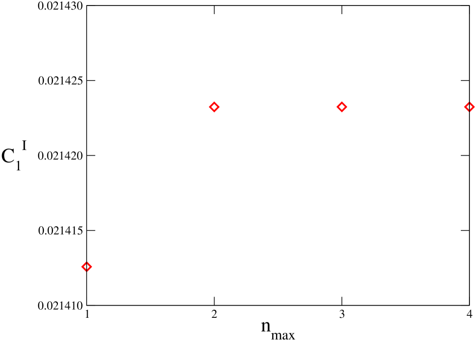
Figure 1: Sensitivity of coefficient $C_{1}^{I}$ as a function of the maximum number of coefficients in the truncated solution, $n_{max}$. The magnitude of the hypermagnetic field in the symmetric phase is $B=0.01$ GeV². The magnitude of the magnetic field in the broken-symmetry phase is $B^{\prime}=\cos\theta_{W}B$. The incoming wave function has quantum numbers $s=0$, $l=1$, an incident energy $E=1.5$ GeV and mass $\mu=1$ GeV. The coupling constant in the symmetric phase is taken as $e_{0}=g^{\prime}=0.344$, whereas in the broken-symmetry phase it is $e_{0}^{\prime}=e=g^{\prime}\cos\theta_{W}$.

In such a case, the matrix representation of the above system of equations can be given in terms of four blocks, each one of size $n_{max}\times n_{max}$,

$$\left(\begin{array}[]{cc}\delta_{n^{\prime\prime}n}&-a_{n^{\prime\prime}n^{\prime}}^{l}\\ k_{n}\delta_{n^{\prime\prime}n}&-k_{n^{\prime}}a_{n^{\prime\prime}n^{\prime}}^{l}\end{array}\right)\left(\begin{array}[]{c}C_{n}^{I}\\ C_{n^{\prime}}^{II}\end{array}\right)=\left(\begin{array}[]{c}-\delta_{n^{\prime\prime}m}\\ k_{m}\delta_{n^{\prime\prime}m}\end{array}\right),$$ (37)

where the upper blocks contain Eqs. (25), (26), and the lower ones Eqs.  (28), (29) (the notation used keeps the $C_{n}^{I}$, $C_{n^{\prime}}^{II}$ indexes), and the terms with $\delta_{n^{\prime\prime}m}$ contain the non-homogenous part, and define the incoming $m$ state.

With the method thus described, we have obtained a quick convergence of the reflection and transmission coefficients as function of $n_{max}$, computed using a set of parameters corresponding to the analysis in the following section. These coefficients do not change after a relatively small value for $n_{max}$ which for the chosen set of parameters corresponds to $n_{max}\sim 20$. The sum of the reflection and transmission coefficients adds up to unity. This point is further discussed in the following sections.

5 Transmission and reflection coefficients

To compute the reflection and transmission coefficients, we consider the a flux of incoming positive-energy particles from region $I$ with definite values of $k_{m}^{i}$ and quantum numbers $s$ and $l$. The conserved current is given by

$$j^{\mu}=\frac{-i}{2}\Psi^{\dagger}{\stackrel{{\scriptstyle\leftrightarrow}}{{\partial^{\mu}}}}\Psi-e_{0}\Psi^{\dagger}\Psi A^{\mu}.$$ (38)

We are interested in the longitudinal component of this current integrated over the transverse $x-y$ plane at $z\rightarrow-\infty$ for the incident and reflected waves and at $z\rightarrow+\infty$ for the transmitted wave, namely

$$j=\int j^{z}dxdy,$$ (39)

where $j$ represents the incident, reflected or transmitted integrated currents

$$j_{i} = k_{m}^{i}$$ (40)

$$j_{r} = \sum_{n}{\rm Re}(k_{n})|C_{n}^{I}|^{2}$$

$$j_{t} = \sum_{n^{\prime}}{\rm Re}(k_{n^{\prime}})|C_{n^{\prime}}^{II}|^{2}.$$

The reflection and transmission coefficients $R$, $T$, are built from the ratio of the reflected and transmitted integrated currents along the $\hat{z}$ direction, to the incident one:

$$R = -j_{r}/j_{i},$$ (41)

$$T = j_{t}/j_{i}.$$ (42)

The incoming wave function corresponds to the first term on the the right-hand side of Eq. (11), whereas the reflected one corresponds to the second and third terms. The transmitted wave function is given by Eq. (24). The coefficients $C_{n}^{I}$, $C_{m}^{I}$ and $C_{n^{\prime}}^{II}$ are found numerically from the solution to Eqs. (25), (26) and (28), (29) by truncating the solution space as described in Sec. 4.

Figure 2 shows $R$ and $T$ for the case of an incoming wave function with quantum numbers $s=0$, $l=1$. The magnitude of the hypermagnetic field in the symmetric phase is $B=0.01$ GeV². The magnitude of the magnetic field in the broken-symmetry phase is obtained from the requirement that the Gibbs free energy be a minimum, and is given by [5]

$$B^{\prime}=\cos\theta_{W}B\,,$$ (43)

where $\theta_{W}$ is Weinberg’s angle. The coupling constant in the symmetric phase is associated to the hypercharge $U(1)_{Y}$ symmetry, so that $e_{0}=g^{\prime}=0.344$. The coupling constant in the broken-symmetry phase is associated to the electromagnetic $U(1)_{em}$, that is, $e_{0}^{\prime}=e=g^{\prime}\cos\theta_{W}$. The mass in the broken-symmetry phase is $\mu=1$ GeV.

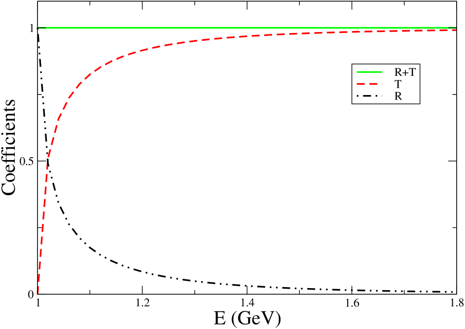
Figure 2: Reflection and transmission coefficients for an incoming wave function with quantum numbers $s=0$, $l=1$. The magnitude of the hypermagnetic field in the symmetric phase is $B=0.01$ GeV². The magnitude of the magnetic field in the broken-symmetry phase is $B^{\prime}=\cos\theta_{W}B$. The coupling constant in the symmetric phase is $e_{0}=g^{\prime}=0.344$, whereas in the broken-symmetry phase it is $e_{0}^{\prime}=e=g^{\prime}\cos\theta_{W}$. The mass in the broken-symmetry phase is $\mu=1$ GeV.

Figure 3 also shows $R$ and $T$ for the same set of parameters as for Fig. 2, except that the magnetic field in the symmetric phase is $B=100$ GeV².

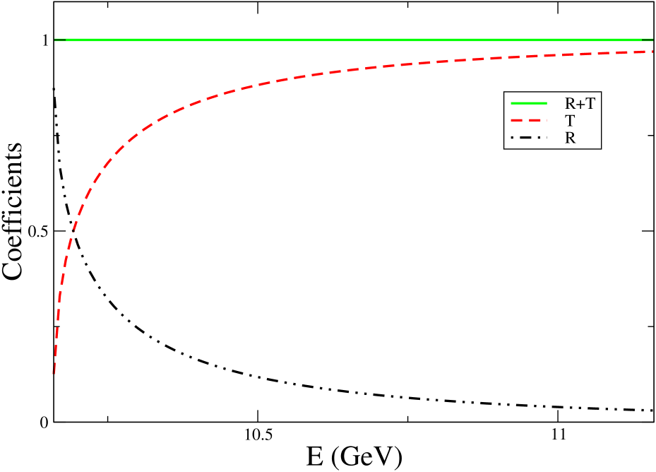
Figure 3: Reflection and transmission coefficients for an incoming wave function with quantum numbers $s=0$, $l=1$. The magnitude of the hypermagnetic field in the symmetric phase is $B=100$ GeV². The magnitude of the magnetic field in the broken-symmetry phase is $B^{\prime}=\cos\theta_{W}B$. The coupling constant in the symmetric phase is $e_{0}=g^{\prime}=0.344$, whereas in the broken-symmetry phase it is $e_{0}^{\prime}=e=g^{\prime}\cos\theta_{W}$. The mass in the broken-symmetry phase is $\mu=1$ GeV.

Notice that in the cases depicted in Figs. 2 and 3, the reflection and transmission coefficients add up to unity, which in the present description of the scattering problem corresponds to the conservation of incoming flux of particles.

To understand such flux conservation, let us recall that, according to Eq. (3), an incoming positive-energy particle from the symmetric phase encounters an effective potential barrier at the interphase of magnitude

$$\Delta V\sim\sqrt{2e_{0}^{\prime}B^{\,\prime}(l+s^{\prime}+1/2)+\mu^{2}}-\sqrt{2e_{0}B(l+s+1/2)}\,,$$ (44)

which, for given quantum numbers of the incident flux, $l$ and $s$, increases with the radial quantum number $s^{\prime}$ of the transmitted wave. Indeed, a one-dimensional version of the problem shows that such flux conservation, notwithstanding the relativistic context, is related to a potential difference that is mass-like. As argued below, this simulates the effect of a non-relativistic Schrödinger equation. We also compare this situation to the case of a gauge-like potential in the time component.

6 Toy models

The conservation of flux can be understood with a simple one-dimensional model where the wave function satisfies the Klein-Gordon equation in two regions with different potentials. With the same conventions for regions $I$ and $II$ as in Sec. 3, we consider

$$[\partial_{t}^{2}-{\partial}_{z}^{2}+V_{1}^{2}]\Psi = 0,\ \ \ z<0$$

$$\left[\partial_{t}^{2}-\partial_{z}^{2}+V_{2}^{2}+\mu^{2}\right]\Psi = 0,\ \ \ z>0,$$ (45)

where $V_{1}$, $V_{2}$ are constant potentials for regions $I$ and $II$, respectively. For $E>V_{1}$ and $E>\sqrt{V_{2}^{2}+\mu^{2}}$ we have propagating incident, reflected, and transmitted momenta $k_{i}=\sqrt{E^{2}-V_{1}^{2}}$, $k_{r}=-k_{i}$, $q_{t}=\sqrt{E^{2}-V_{2}^{2}-\mu^{2}}$, respectively.

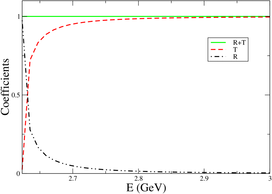
Figure 4: Reflection and transmission coefficients in the one-dimensional with mass-like one-dimensional potential in Eq. (48), with $V_{1}=2.6$ GeV in region $z<0$, and $V_{2}=2.3$ GeV in region $z>0$. The reflection and transmission coefficients add to one. The mass in the $z>0$ region is $\mu=1$ GeV.

Using the explicit form for the conserved current given in Eq. (38), and assuming an incoming flux of positive-energy particles from region $I$, the reflection and transmission coefficients are given by

$$R = \frac{(k_{i}-q_{t})(k_{i}-q_{t})^{*}}{(k_{i}+q_{t})(k_{i}+q_{t})^{*}},$$

$$T = \frac{4k_{i}^{2}}{(k_{i}+q_{t})(k_{i}+q_{t})^{*}}\ ;$$ (46)

these correspond to the ratio of the reflected ($r$) and transmitted ($t$) currents to the incident one, along the $\hat{z}$ axis

$$j_{zr}/j_{zi} = -R$$

$$j_{zt}/j_{zi} = T\ {\rm Re}(q_{t})/k_{i},$$ (47)

where the normalization is taken to the same density $j_{0}$ as in Eqs. (38) for all cases. As shown in Fig. 4, we get current conservation in this case, which we associate with the Schrödinger form of Eq. (6).

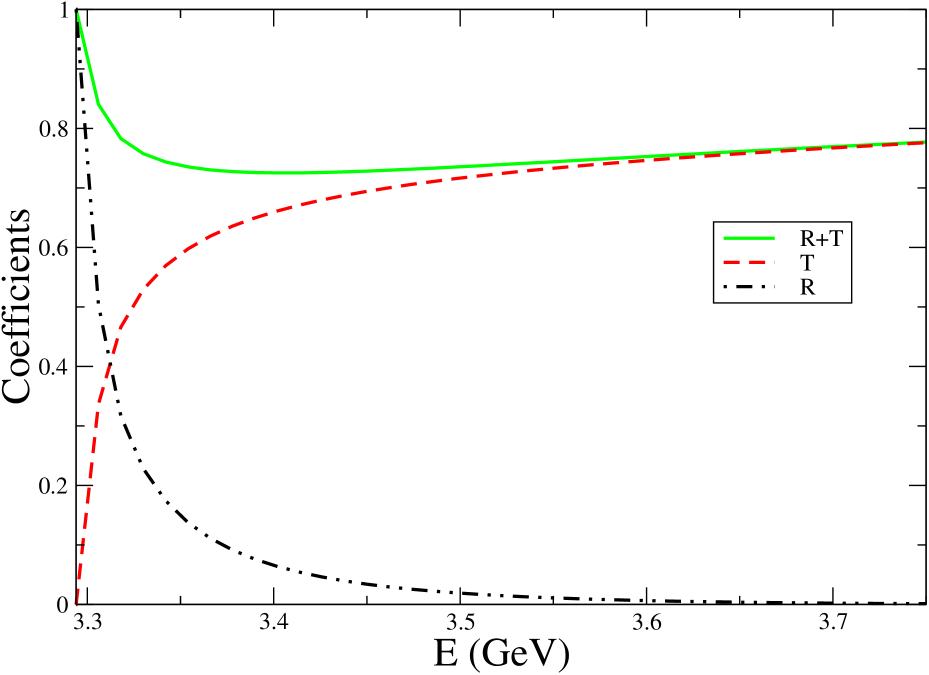
Figure 5: Reflection and transmission coefficients with gauge-like one-dimensional potential in Eq. (6), and $V_{1}=2.6$ GeV in region $z<0$, and $V_{2}=2.3$ GeV in region $z>0$. The reflection and transmission coefficients add to one only in the non-relativistic and ultra-relativistic limits. The mass in the $z>0$ region is $\mu=1$ GeV.

This is not the case for a gauge-like potential in the time derivative, as in

$$[(i\partial_{t}-V_{1})^{2}-{\partial}_{z}^{2}]\Psi = 0,\ \ \ z<0$$

$$\left[(i\partial_{t}-V_{2})^{2}-\partial_{z}^{2}+\mu^{2}\right]\Psi = 0,\ \ \ z>0,$$ (48)

where $V_{1}$, $V_{2}$ are constant potentials for regions $I$ and $II$, respectively. For $E>V_{1}$ and $E>V_{2}+\mu$ we have propagating incident, reflected, and transmitted momenta $k_{i}=E-V_{1}$, $k_{r}=-k_{i}$, $q_{t}=\sqrt{(E-V_{2})^{2}+\mu^{2}}$, respectively. The currents are

$$j_{zr}/j_{zi} = -R$$

$$j_{zt}/j_{zi} = \frac{E-V_{1}}{E-V_{2}}T\ {\rm Re}(q_{t})/k_{i},$$ (49)

where $T$, $R$ are still those of Eqs. (46). It follows that within the positive-energy solution approximation used, the flux conservation $j_{xi}=j_{xr}+j_{xt}$ is valid only in the non-relativistic limit, and the ultra-relativistic limit $E\rightarrow\infty$, as shown in Fig. 5. The flux non-conservation in the intermediate regime is associated to particle-pair creation. The trouble comes from the relativistic normalization in Eq. (6). In practice, this means that a particle encounters a potential that makes possible the opening of additional channels contributing to the scattering processes, such as pair production.

Such anomalous behavior is already known to arise in the context of the Dirac equation in the treatment of scattering and is called Klein paradox [14]. This signals the need to account for negative-energy solutions. In fact, the gauge-like potential in Eqs. (48) and the current in Eq. (38) produce the different current terms in Eq. (6). It follows that the hypermagnetic-field problem resembles the first, Schrödinger-like, case.

7 Conclusions

In this work, we presented the exact solution for the scattering problem of scalar particles propagating within two regions of different but constant magnetic fields, separated by a planar interphase. The fields are assumed to be perpendicular to the interphase, while the solution for arbitrary directions is briefly explained in the Appendix. The two regions are defined by the condition that the particle is massless on one side of the interphase and massive on the other, such as during a first-order EWPT, outside and inside the nucleated bubbles, respectively.

In the general case in which the direction of the magnetic field is not perpendicular to the wall interphase, we can decompose it into normal and parallel components. Recall that the normal component of the external field is continuous across the interphase and also that charged-particle trajectories consist of an overall displacement along the field lines superimposed to circular motion around the field lines. The relevant physical effect of the magnetic-field component directed along the wall is its ability to capture low momentum particles upon scattering since these can make transitions to states that can remain orbiting filed lines in this direction close to the wall.

In order to estimate the magnitude of such fields able to capture particles on the wall, let us look at the following classical argument: Equilibrium between the Lorentz force and the centrifugal force gives for the radius of the orbit for a particle trapped in the wall $R=p/(eB)$ where $p$ is the particle’s momentum, $e$ is its charge and $B$ the strength of the magnetic field. Considering the physical situation of a wall with a finite thickness $\lambda$, let us take $R\sim\lambda$. Also, let us parameterize the strength of the magnetic field as $B=bT^{2}$, where $b$ is a dimensionless factor and $T$ is the temperature, then $b\sim p/(e\lambda T^{2})$. Taking the momentum of a typical particle to be of order of the temperature $T$, namely $p\sim T$ and since $\lambda\sim T^{-1}$ (see for example Ref. [8]), we obtain $b\sim{\mathcal{O}}(10)$ which is already a very high value of the magnetic field. Although uncertainties on the strength of the magnetic fields at the EWPT are large, it is safe to assume that $b\ll 10$ (see for example Ref. [5], and references therein).

We see that the loss of flux in these trapped modes for small field strengths is small, and therefore that the relevant magnetic-field component for the computation of transmission and reflection coefficients is the normal one, thus the magnetic field chosen in this paper. It is also worth mentioning that for a wall with non-zero thickness, realistic boundary conditions for the external gauge field imply the existence of a magnetic-field component along the direction of the wall and localized within the dimensions of the wall (see the discussion in Sec. IV of the second of Ref. [7]). In this case, similar arguments apply and the conclusion is that only very intense fields are able to produce an effect that involves a component of the magnetic field parallel to the wall.

The problem at hand is solved through continuity conditions on a surface, rather than a point. The solution involves the expression of the wave function on one side of the interphase as a superposition of the complete set of solutions on the other side, and the continuity of the wave function and its derivative across the interphase. In order to numerically solve the problem, we resorted to a truncation of the system of equations involving the coefficients of the expansion.

We found that in such a scheme, the flux of particles is conserved, which we associate with the Schrödinger nature of the magnetic-field equation. We showed in a simple one-dimensional model that such flux conservation can be understood as arising from the contribution of an effective mass-like potential barrier associated to momentum and radial modes, while, in the case of a gauge-like potential in the time component, the Klein paradox [14], signals the need to account for negative-energy solutions.

As previously found [7, 9], the scattering of chiral fermions during a first-order EWPT gives rise to an axial asymmetry that can be subsequently converted into a baryon asymmetry. The description of the scattering process used simplifying assumptions for the reflected and transmitted states. It will thus be interesting to explore the consequences of the exact method introduced in this work in the context of the Dirac equation on the generated axial asymmetry. This is work under progress, and will be reported as a sequel of the present one.

References

- [1] K. Enqvist, Int. J. Mod. Phys. D 7, 331 (1998), astro-ph/9803196; R. Maartens, Pramana 55, 575 (2000), astro-ph/0007352; D. Grasso and H.R. Rubinstein, Phys. Rep. 348 163, (2001), astro-ph/0009061; M. Giovannini, Int. J. Mod. Phys. D 13, 391-502 (2004), astro-ph/0312614.
- [2] P. Cea, G.L. Fogli and L. Tedesco, Mod. Phys. Lett. A 15, 1755 (2000), astro-ph/0007053; L. Campanelli, P. Cea, G.L. Fogli and L. Tedesco, Phys. Rev. D 65, 085004 (2002), astro-ph/0111327; L. Campanelli, G.L. Fogli and L. Tedesco, ibid 70, 083502 (2004), astro-ph/0409077.
- [3] A. Ayala, A. Sánchez, G. Piccinelli and S. Sahu, Phys. Rev. D 71, 023004 (2005), hep-ph/0412135.
- [4] M. Giovannini and M. E. Shaposhnikov, Phys. Rev. D 57, 2186 (1998), hep-ph/9710234.
- [5] P. Elmfors, K. Enqvist and K. Kainulainen, Phys. Lett. B 440, 269 (1998), hep-ph/9806403.
- [6] see for example: M.S. Turner and L.M. Widrow, Phys. Rev. D 37, 2743 (1988); A.-C. Davis and K. Dimopoulos, ibid 55, 7398 (1997); B. Ratra, Astrophys. J. Lett. 391, L1-L4 (1992).
- [7] A. Ayala, J. Besprosvany, G. Pallares and G. Piccinelli, Phys. Rev. D 64, 123529 (2001), hep-ph/0107072; A. Ayala, G. Piccinelli and G. Pallares, ibid 66, 103503 (2002), hep-ph/0208046.
- [8] A. Ayala, J. Jalilian-Marian, L. McLerran and A. P. Vischer, Phys. Rev. D 49, 5559 (1994).
- [9] A. Ayala and J. Besprosvany, Nucl. Phys. B, 651, 211 (2004), hep-ph/0211234.
- [10] A.A. Sokolov and I.M. Ternov, Radiation from Relativistic Electrons (American Institute of Physics, New York 1986).
- [11] J. Besprosvany and M. Moreno, Rev. Mex. Fis. 50, 366 (2004), hep-th/0105280.
- [12] M. Abramowitz, Handbook of mathematical functions, Dover, New York, 1965.
- [13] I. S. Gradshteyn and I. M. Ryzhik, Table of integrals, series and products, Academic, Boston, 1994.
- [14] O. Klein, Z. Phys. 53, 157 (1929).