Implementing the ME+PS merging algorithm

Abstract:

The method to merge matrix elements for multi particle production and parton showers in $e^{+}e^{-}$ annihilations and hadronic collisions and its implementation into the new event generator SHERPA is described in detail. Examples highlighting different aspects of it are thoroughly discussed, some results for various cases are presented. In addition, a way to extend this method to general electroweak interactions is presented.

agraphs

1 Introduction

The analysis of multi-particle final states becomes increasingly important in the search for the production and decay of new, heavy particles. Therefore, in order to guide such analyses, their simulation in Monte Carlo event generators should be as correct as possible. There are two complementary approaches to model the production of multi-particle final states: First, employing fixed-order perturbation theory, exact matrix elements at tree-level or beyond describe particle production in specific processes through Feynman diagrams, taking into account all quantum interferences at the corresponding level of accuracy. Alternatively, the parton shower approach organises the emission of secondary partons in such a way that all leading collinear or soft logarithms of the form $\alpha_{S}^{n}\log^{2n}$ are resummed. The former way of modelling particle production has the benefit of being well-defined and exact up to given fixed-order accuracy for large angle or high energy emission of partons, whereas the second approach correctly treats the soft and collinear regions of phase space. Of course, a combination of both approaches allows for a better description of particle production over the full available phase space. A way of merging multi-particle matrix elements at tree-level with the subsequent parton shower consistently at leading logarithmic accuracy and taking into account important parts of the next-to leading logarithms was formulated first for the process $e^{+}e^{-}\to$hadrons in [1]. The principles of its application to hadronic processes have been discussed in [2]. In both cases, the phase space of particle production is divided into two disjoint regimes, one of jet production covered by the corresponding matrix elements, and one of jet evolution modelled through the parton shower. The separation in both cases, $e^{+}e^{-}\to$hadrons and hadronic collisions, is achieved through a $k_{\perp}$ jet measure [3, 4, 5]. The implementation of this algorithm is discussed in detail in this publication; it forms the cornerstone of the new event generator SHERPA [6]. The approach been extended [7] to cover also the dipole shower formulation of multiple parton emission [8]. A somewhat related approach has been taken in [9]. The algorithm has been tested in a variety of versions, ranging from its prime example $e^{+}e^{-}\to$hadrons [10] over the production of gauge bosons in hadronic collisions at the Tevatron [11, 12] or the LHC [13] to $W$-pair production at the Tevatron [14].

To some extent, however, all existing algorithms so far assume that there is a signal process (like, e.g., $e^{+}e^{-}\to q\bar{q}$ or $q\bar{q}\to l\bar{\nu}_{l}$) with one specific order in the electroweak coupling constant and that all additional jets are emitted through strong interactions. This implies that all matrix elements have the same order in the electroweak coupling constant and that they form a hierarchy of extra orders in $\alpha_{s}$, related to extra jets. Despite its apparent success there is one question that remains to be answered. This is the question of how to deal with situations where both electroweak and strong amplitudes contribute significantly to the same final state. For example, at LEP II both pure QCD amplitudes and $W$ boson pair production amplitudes contribute to the total cross section of 4-jet production processes. Depending on the specific kinematical situation, their relative amount may vary; however, they exhibit different properties. This is exemplified by their colour flows, being responsible for the kinematical domain in which hadrons are formed. It is clear that a consistent merging procedure for such processes is highly desirable. Such a merging algorithm has to take proper care of relevant coupling constants, and it has to reliably predict the corresponding colour structure.

In the next section, Sec. 2, the algorithm is discussed for both $e^{+}e^{-}$ and hadronic processes. Certain aspects presented here have not been covered before. They include the treatment of jet production beyond the availability of corresponding matrix elements and some ways of using variable jet resolution scales for different jet multiplicities. In addition, some first steps into the direction of treating matrix elements, where electroweak and strong interactions compete with each other are reported. The presentation proceeds with examples highlighting the ideas underlying the algorithm, cf. Sec. 3. Finally, a large amount of results indicating its quality are presented in Sec. 4. Details on the specific implementation of the algorithm into SHERPA are given in the appendix, Sec. A.

2 The algorithm

In this section the merging algorithm together with its extensions, as implemented in SHERPA, will be discussed. It can be divided into three parts. First of all, a sample of matrix elements has to be defined, from which processes are selected for the generation of individual events. The four-momenta of the particles are distributed according to the corresponding matrix element. Then, having fixed the number, flavours and four-momenta of the particles, a pseudo parton shower history is constructed through backwards clustering of the particles according to the $k_{\perp}$ algorithm. Here, care has to be taken in situations, where one particular clustering allows for different colour flows. The nodal values of this clustering serve as input for the construction of a weight applied on the matrix element. This weight resums higher order effects at leading logarithmic accuracy and consists of Sudakov form factors for coloured lines (e.g., quarks or gluons) and of ratios of the strong coupling constant. If the event is accepted, parton showers are attached to the outgoing particles. For this, again the nodes of the clustering serve as input. Inside the parton shower, those emissions are vetoed that lead to additional unwanted jets. At this point there is some subtlety, since it is obviously impossible to calculate matrix elements for an infinite number of additional jets. Hence, there is some maximal number $n_{\rm max}$ of jets covered by the matrix elements, higher jet multiplicities must be accounted for by the parton shower. This leads to a somewhat modified treatment of the parton shower for those events with $n_{\rm max}$ jets stemming from the matrix elements.

Apart from this special treatment for configurations with the largest number of jets produced through matrix elements, there are cases where a similar treatment is necessary for configurations with the minimal number of jets. Examples include both electroweak such as $e^{+}e^{-}\to W^{+}W^{-}\to jets$ and the QCD production of jets in hadronic collisions. Using the $k_{\perp}$ measure to separate matrix elements with the minimal number of jets $n_{\rm min}$ from higher jet multiplicities with $n>n_{\rm min}$ also restricts the phase space for the minimal number of jets. Since the separation of different jet multiplicities is slightly washed out by the parton shower and hadronisation, the lowest jet multiplicity samples experience a loss of events at the phase space boundary, which is not compensated for by smaller jet multiplicities. To deal with this problem one may try to use generation cuts that are much tighter than the analysis cuts - an option that is clearly not very efficient. Alternatively, a lower jet definition cut may be used for the lowest jet multiplicity. This idea leads to an extension of the algorithm, which enables a merging of processes with different jet multiplicities and different separation cuts. In fact, this algorithm is closely related to the highest multiplicity treatment.

In the following, the algorithm and some of its refinements are discussed in greater detail, dividing the procedure into three steps, namely matrix element generation, parton clustering and Sudakov weight construction and into, finally, running the parton showers.

2.1 Combination of matrix elements

1. Composition of the process samples:
   In each run, processes with a fixed identical number of electroweak couplings may be combined, which differ only in the number of extra jets produced through QCD. All strongly interacting particles are subject to phase space cuts according to the $k_{\perp}$ algorithm [3, 4, 5]. This is necessary in order to allow a reweighting of the matrix element with Sudakov form factors. Phase space cuts on other particles are not needed unless for the sake of avoiding potential infrared divergencies. As an example consider the case of a (massless) lepton pair, which have to be cut through, e.g. a cone algorithm or by demanding some minimal invariant masses.

   In the original algorithm, however, it was implicitly assumed that any gauge boson of the electroweak interactions is connected to maximally one strongly interacting line only; in other words, it was implicitly assumed that any photon, $W$ or $Z$ boson would couple to one quark line only. The present proposal aims at widening the scope in such a way that competition between strong and electroweak interactions is possible.

2. Selection of a particular process:
   For all the processes contributing in a single run, labelled with $i$, total cross sections are evaluated at tree-level through

   $$\sigma_{i}^{(0)}=\int{\rm d}\Omega|{\cal M}(\mu_{R},\,\mu_{F})|^{2}\,,$$ (1)

   where ${\rm d}\Omega$ denotes the integral over the available phase space. For convenience, here any eventual integration over the Bjorken-$x$ of incoming partons is subsumed in ${\rm d}\Omega$. The matrix element ${\cal M}$ eventually is extended by parton distribution functions; it is evaluated at $\mu_{R}=\mu_{F}=Q_{\rm cut}$, the cut parameter of the $k_{\perp}$ algorithm.

   The probability ${\cal P}_{i}$ for a process $i$ to be selected for event generation is then given by

   $${\cal P}_{i}^{(0)} =\frac{\sigma_{i}^{(0)}}{\sum_{j}\sigma_{j}^{(0)}}\,.$$ (2)

   Having selected the process, four-momenta for the incoming and outgoing particles are chosen according to its matrix element.

3. Highest multiplicity treatment:
   For those processes that have the highest multiplicity of jets in the matrix element, i.e. where $n=n_{\rm max}$, already during integration the scale $Q_{s}$ of the softest jet produced through QCD is determined according to the $k_{\perp}$ algorithm. Then, the parton distribution functions in the matrix element are taken at the factorisation scale $\mu_{F}=Q_{s}$, whereas the renormalisation scale used in the evaluation of the coupling constant remains at $\mu_{R}=Q_{\rm cut}$. Of course, this will later on affect the Sudakov weights and the parton showering as well; at that point, however, it implicitly takes into account the possibility of having softer extra jets emitted in the initial state parton shower.

4. Multi-cut treatment:
   There is some condition that the multi-cut treatment does not lead to ambiguities, namely that the jet definition becomes tighter with increasing jet multiplicity. In other words, for each jet multiplicity $n$, a jet separation cut $Q_{\rm cut}^{(n)}$ is defined such that $Q_{\rm cut}^{(n-1)}\leq Q_{\rm cut}^{(n)}$. For the calculation of the corresponding a priori cross sections $\sigma^{(n)}$ the factorisation scales are also set dynamically to

   $$\mu_{F}=Q_{\rm min}=\mbox{\rm min}\left\{Q_{s},Q_{\rm cut}^{(n+1)}\right\}\,,$$ (3)

   where $Q_{s}$ is the scale of the softest jet in the process. Again, the renormalisation scale is fixed at $\mu_{R}=Q_{\rm cut}^{(n)}$.

2.2 Pseudo parton shower history

1. Clustering of particles:
   In the original version of the merging procedure, only QCD clusterings have been considered. There, for each allowed pair of partons a relative transverse momentum has been defined. According to the $k_{\perp}$ algorithm, its square reads

   $$Q_{ij}^{2} =2\,\mbox{\rm min}\{E_{i}^{2},E_{j}^{2}\}(1-\cos\theta_{ij})$$ (4)

   for a pair of partons in $e^{+}e^{-}$ collisions. In hadronic collisions it is given by

   $$Q_{ij}^{2} =2\,\mbox{\rm min}\{p_{\perp,i}^{2},p_{\perp,j}^{2}\}\,\left[\cosh^{2}(\eta_{i}-\eta_{j})-\cos^{2}(\phi_{i}-\phi_{j})\right]$$ (5)

   for the clustering of two final state hadrons, and by

   $$Q_{i}^{2} =p_{\perp,i}^{2}$$ (6)

   when a final state parton is to be clustered with an initial state particle. In the original algorithm, the pair with the lowest $k_{\perp}$ has been clustered. In order to prohibit “illegal” clusterings, such as, for instance, the clustering of two quarks instead of a quark-anti-quark pair, only those pairs have been considered that correspond to a Feynman diagram contributing to the process in question.

   Going beyond this, some new problems may manifest themselves, which are related to the possibility of having competing colour flows. A good example for this is the possible competition of clustering a quark-anti-quark pair into either a gluon or a $Z$-boson. To resolve this ambiguity, there are, in principle, two options: One would be to globally select a specific colour configuration according to the relative weight of different colour-ordered amplitudes. This is clearly the preferred choice. The other one, that will be pursued as a proposal here, is to try to decide locally which colour configuration to chose.

   For this, relative weights are constructed for each possible clustering, which take into account the coupling and pole structure of the underlying Feynman diagram(s). In each case, the contribution ${\cal W}_{ij}$ to the weight for a specific clustering of two particles $ij\to k$ can be written as

   $${\cal W}_{ij;k}(q) =\frac{[g_{ij}(\mu_{R})g_{kl}(\mu_{R})]^{2}}{(q^{2}-m_{k}^{2})^{2}+m_{k}^{2}\Gamma_{k}^{2}}\,,$$ (7)

   where $g_{ij}(\mu_{R})$ is the coupling constant at the vertex and $g_{kl}(\mu_{R})$ denotes the coupling constant of the resulting propagator in the potential next clustering $kl\to m$. In addition, the propagator term contains the mass and the (fixed) width of particle $k$. Clearly, $m_{k}$ and $\Gamma_{k}$ may be zero, for instance for gluons or massless quarks. In the equation above, $q^{2}$ is the square of the four-momentum $q$ of the pair $ij$.

   Now, for each allowed clustering of pairs $ij$, all potential ${\cal W}_{ij}(q)$ with different coupling structure are added, and the pair with the largest total weight

   $${\cal W}_{ij}^{\rm tot}(q) =\sum\limits_{k}{\cal W}_{ij;k}(q)$$ (8)

   is selected. The emerging propagator $k$ is then chosen according to the relative probability

   $${\cal P}_{k} =\frac{{\cal W}_{ij;k}(q)}{{\cal W}_{ij}^{\rm tot}(q)}\,.$$ (9)

2. Core $2\to 2$ process:
   In the original as well as in the extended version of the merging algorithm, proposed here, this clustering procedure is repeated recursively, until a core $2\to 2$ process is recovered. It defines the initial colour flow in the large $N_{c}$ limit necessary for the fragmentation. In addition, through this choice of an initial colour flow, the hard process scales $Q_{h}$ for the partons in this process are defined. The following cases must be considered:

   • Two particles with and two particles without colour quantum number, for instance $e^{+}e^{-}\to q\bar{q}$, $q\bar{q}\to e^{+}e^{-}$, or $gg\to H\to\tau\tau$ in an effective model for the $ggH$ coupling. Then, for the two coloured objects, $Q_{h}^{2}=\hat{s}$.

   • Three particles with colour quantum numbers and one without, for instance in $q\bar{q}\to Wg$. Then, for the incoming particles $Q_{h}^{2}=\hat{s}$, and for the outgoing ones $Q_{h}$ is given by their transverse momentum.

   • Four particles with colour. In this case, often different colour structures are competing. The selection is then made according to relative contributions which can usually be connected with the $\hat{s}$, $\hat{t}$ or $\hat{u}$ channel exchange of colour. The hard scale for all four particles is then chosen according to this selection. Hence, usually, the minimum of $\hat{u}$ and $\hat{t}$ is the relevant scale.

3. Construction of the Sudakov weight:
   Having fixed the parton shower sequence and the hard scales $Q_{h}$, the Sudakov weight can be calculated. To a large extent, the construction prescription for this is the same for the original approach as well as for its proposed extension. In both cases, the Sudakov weights consists of ratios of the strong coupling constant taken at the varying nodal scales and at the fixed renormalisation scale and of Sudakov form factors, which in next-to-leading logarithmic (NLL) approximation are given by

   $$\Delta(Q,Q_{0})=\exp\left[-\int\limits_{Q_{0}}^{Q}{\rm d}q\Gamma(Q,q)\right]\,.$$ (10)

   Here, $\Gamma(Q,q)$ is the integrated splitting function for the particle in question. For convenience, it incorporates a factor $\alpha_{S}(q)/q$. Integrated splitting functions for different splittings are listed in the appendix. In terms of these constituents the Sudakov weight is constructed as a product of

   • factors $\alpha_{S}(Q)/\alpha_{S}(\mu_{R})$ for each node with $Q=k_{\perp}$ which involves a strong coupling constant;

   • factors $\Delta(Q_{1},Q_{\rm cut})/\Delta(Q_{2},Q_{\rm cut})$ for each internal line (propagator) that carries colour quantum numbers, where the arguments are given by the nodal $k_{\perp}$ scales $Q_{1}$ and $Q_{2}$;

   • and of factors $\Delta(Q_{1},Q_{\rm cut})$ for colour-charged outgoing lines emerging at a node with $Q_{1}=k_{\perp}$.

   At this point it should be noted that in such cases where coloured particles are produced through $s$-channel electroweak interactions the nodal scale value of the vertex should be the invariant mass $\hat{s}$ of the particles rather than their transverse momentum, which again is beyond the scope or the original algorithm.

4. Highest multiplicity treatment:
   In case, a hard process with the maximal number of jets accommodated by the matrix elements has been chosen, the parton shower must be able to produce higher jet configurations. Of course, these additional jets may in principle emerge at transverse momenta larger than the jet definition cut $Q_{\rm cut}$. On the other hand, it is clear that they should be softer than the softest jet produced by the matrix element in order to ensure that the matrix element is used to cover the hard regions of phase space. Since the Sudakov form factors forming the weight attached to the matrix elements can be identified as a no-radiation probability between two scales, the soft scales of the Sudakov form factors need to be modified. Because in this situation radiation from the parton shower must be softer than $Q_{s}$, the scale of the softest jet in the matrix element, rather than $Q_{\rm cut}$, this modification amounts to a replacement $Q_{\rm cut}\to Q_{s}$ in all Sudakov form factors, i.e. for both internal and external lines.

5. Multi-cut treatment:
   Similarly to the highest multiplicity treatment discussed above, in the multi-cut treatment the soft scales of the Sudakov weight are also set dynamically, i.e. in dependence on the actual kinematical configuration. The scale $Q_{\rm cut}$ in the Sudakov form factors for an $n$ jet process is replaced by $Q_{\rm min}$ defined according to Eq. (3). In case the process is purely electroweak, like $e^{+}e^{-}\to ZZ\to q\bar{q}q\bar{q}$, this prescription translates into completely switching off all Sudakov form factors if $Q_{s}\leq Q_{\rm cut}^{(n+1)}$.

2.3 Starting the parton shower

1. Vetoing emissions:
   According to the paradigm of the merging procedure, inside the parton shower all emissions leading to extra unwanted jets are vetoed. This is implemented in the following way:

   • The probability for no branching resolvable at a scale $t_{0}$, usually the infrared cut-off of the parton shower, between two scales $t_{1}$ and $t_{2}$ is given by the ratio

     $${\cal P}_{\rm no}(t_{1},t_{2})=\frac{\Delta(t_{1},t_{0})}{\Delta(t_{2},t_{0})}$$ (11)

     of Sudakov form factors. Equating this with a random number allows to solve this for $t_{2}$, the scale of the next trial emission.

   • Having at hand the transverse momentum related to this trial emission, it can be compared with the jet resolution of the $k_{\perp}$ algorithm. If this particular emission would give rise to an unwanted jet, the next trial emission is constructed with its upper scale $t_{1}$ equal to the actual scale $t_{2}$ of the vetoed emission.

   For a single parton line starting at some scale $Q$ the matrix element correction weight reads

   $$W_{\rm ME}=\Delta(Q,Q_{\rm cut})\,.$$ (12)

   The combined weight of all possible rejections due to vetoed emissions in the parton shower for the same parton, starting at scale $Q$ at NLL accuracy reads

   $$W_{\rm PS}=\left[1+\int\limits_{Q_{\rm cut}}^{Q}{\rm d}q\Gamma(Q,q)+\int\limits_{Q_{\rm cut}}^{Q}{\rm d}q\Gamma(Q,q)\int\limits_{Q_{\rm cut}}^{q}{\rm d}q^{\prime}\Gamma(Q,q^{\prime})+\dots\right]=\Delta^{-1}(Q,Q_{\rm cut})\,.$$ (13)

   Combining both thus formally leads to a cancellation of large logarithms of the form $\log Q/Q_{\rm cut}$ at NLL precision. However, there are remaining dependencies on $Q_{\rm cut}$, some of which are due to the fact that the actual implementation of the parton shower is at a different level of logarithmic accuracy.

   For the highest multiplicities or for the multi-cut treatment, the veto of course is performed w.r.t. $Q_{s}$ or $Q_{\rm min}$, respectively. In case the process is purely electroweak no shower veto is applied at all as long as $Q_{\rm min}\leq Q_{\rm cut}$.

2. Starting scales:
   The reasoning above immediately implies which starting scales are to be chosen for the parton shower evolution of each parton. In each case it should be the scale where the parton was first produced, in accordance with how the Sudakov weights are constructed and how the vetoing applied in the parton shower cancels the dependence on the jet resolution scale.

   There is one last minor point to be discussed, namely the scale, at which the parton density functions are evaluated in the backward evolution of initial state showers. Remember that there, in order to recover the correct parton distribution functions at each step of the space-like evolution, the ratio of Sudakov form factors describing the no-branching probability between $t_{1}$ and $t_{2}$ are supplemented with corresponding factors, namely,

   $${\cal P}_{\rm no}(t_{1},t_{2})=\frac{f(x,\,t_{2})}{f(x,\,t_{1})}\cdot\frac{\Delta(t_{1},t_{0})}{\Delta(t_{2},t_{0})}\,.$$ (14)

   If this expression is to describe the first emission through the parton shower along an incoming parton line, the hard scale $t_{1}$ in the parton distribution function is replaced by either $Q_{\rm cut}$ (or $Q_{s}$ or $Q_{\rm min}$, if the process in question has the maximal number of jets in the matrix element, or if the multi-cut treatment is active).

3 Examples

In this section, the algorithms discussed above are illustrated through some examples, namely

1. $e^{+}e^{-}\to\mbox{jets}$,

2. $p\bar{p}\to W+\mbox{jets}$ ,

3. $p\bar{p}\to\mbox{jets}$ , and

4. $e^{+}e^{-}\to d\bar{d}u\bar{u}(g)$.

3.1 Example I – $e^{+}e^{-}\to\mbox{jets}$

As a first example for the original version of the algorithm, consider the process $e^{+}e^{-}\to\mbox{jets}$ at LEP I. Choosing a jet resolution of $Q_{\rm cut}=5.77$ GeV ($y_{\rm cut}=0.004$ in the Durham scheme), the a-priori cross sections $\sigma^{(0)}_{i}$ and the resulting effective cross sections $\sigma_{i}=\sigma^{(0)}_{i}\cdot W_{\rm ME}$ for a specific choice of $\alpha_{S}=0.127$ are given by

$$\begin{array}[]{l@{\,=\,}r@{\extracolsep{15mm}} l@{\extracolsep{1mm}\,=\,}r@{\extracolsep{15mm}} l@{\extracolsep{0mm}\,=\,}r}\sigma_{2}^{(0)}&40.46\,\mbox{\rm nb&\sigma_{2}^{\rm nmax=5}&18.80\,\mbox{\rm nb&({\cal R}_{2}&38.8\%)\\ \sigma_{3}^{(0)}&43.38\,\mbox{\rm nb&\sigma_{3}^{\rm nmax=5}&21.10\,\mbox{\rm nb&({\cal R}_{3}&43.5\%)\\ \sigma_{4}^{(0)}&14.05\,\mbox{\rm nb&\sigma_{4}^{\rm nmax=5}&6.90\,\mbox{\rm nb&({\cal R}_{4}&14.2\%)\\ \sigma_{5}^{(0)}&2.80\,\mbox{\rm nb&\sigma_{5}^{\rm nmax=5}&1.69\,\mbox{\rm nb&({\cal R}_{5}&3.5\%)\\ \lx@intercol\hfil\hfil\lx@intercol&\sigma_{\rm tot}^{\rm nmax=5}&\lx@intercol\sum\limits_{i=2}^{5}\sigma_{i}^{\rm nmax=5}=48.49\,\mbox{\rm nb}\hfil\lx@intercol\end{array}}}}}}}}}$$

Assume now that at some point a three-jet event is chosen with a $q\bar{q}g$ final state. The diagrams contributing to this process are depicted in Fig. 1.

Figure 1: The diagrams contributing to $e^{+}e^{-}\to 3\mbox{jets}$.

There are two allowed clusterings, namely $qg$ and $\bar{q}g$. If the former leads to a smaller $k_{\perp}$, i.e. if $Q(qg)<Q(\bar{q}g)$ this clustering is selected, of course with scale $Q_{1}=Q(qg)$, and the core $2\to 2$ process is readily recovered. Its associated hard scale is $Q=\sqrt{s}$. The Sudakov weight is constructed, leading to

$${\cal W}_{\rm ME} =\Delta_{\bar{q}}(Q,Q_{\rm cut})\,\frac{\Delta_{q}(Q,Q_{\rm cut})}{\Delta_{q}(Q_{1},Q_{\rm cut})}\,\frac{\alpha_{S}(Q_{1})}{\alpha_{S}(Q_{\rm cut})}\,\Delta_{q}(Q_{1},Q_{\rm cut})\Delta_{g}(Q_{1},Q_{\rm cut})$$

$$=\Delta_{\bar{q}}(Q,Q_{\rm cut})\,\Delta_{q}(Q,Q_{\rm cut})\,\frac{\alpha_{S}(Q_{1})}{\alpha_{S}(Q_{\rm cut})}\,\Delta_{g}(Q_{1},Q_{\rm cut})\,,$$ (15)

where the first factor in the first line corresponds to the anti-quark line, the second factor is for the internal quark line, the ratio of the strong coupling constants applies for the vertex, and the two last factors correspond to the two outgoing lines. Emissions in the parton shower for all three lines are vetoed if their transverse momentum is larger than $Q_{\rm cut}$; the start scales for the parton shower evolution are $t$ for both the quark and the anti-quark line, and $t_{1}$ for the gluon.

If, in contrast in the simulation the matrix elements are restricted by $n_{\rm max}=3$, the highest multiplicity treatment would apply to the three-jet configuration. Consequently, the cross sections and rates change according to

$$\begin{array}[]{l@{\,=\,}r@{\extracolsep{15mm}} l@{\extracolsep{1mm}\,=\,}r@{\extracolsep{15mm}} l@{\extracolsep{0mm}\,=\,}r}\sigma_{2}^{(0)}&40.46\,\mbox{\rm nb&\sigma_{2}^{\rm nmax=3}&18.80\,\mbox{\rm nb&({\cal R}_{2}&36.3\%)\\ \sigma_{3}^{(0)}&43.38\,\mbox{\rm nb&\sigma_{3}^{\rm nmax=3}&32.94\,\mbox{\rm nb&({\cal R}_{3}&63.7\%)\\ \lx@intercol\hfil\hfil\lx@intercol&\sigma_{\rm tot}^{\rm nmax=3}&\lx@intercol\sum\limits_{i=2}^{3}\sigma_{i}^{\rm nmax=3}=51.74\,\mbox{\rm nb}\,,\hfil\lx@intercol\end{array}}}}}$$ (16)

and the weight for the three-jet configuration would be given by

$$\tilde{\cal W}_{\rm ME} =\Delta_{\bar{q}}(Q,Q_{1})\,\frac{\Delta_{q}(Q,Q_{1})}{\Delta_{q}(Q_{1},Q_{1})}\,\frac{\alpha_{S}(Q_{1})}{\alpha_{S}(Q_{1})}\,\Delta_{q}(Q_{1},Q_{1})\Delta_{g}(Q_{1},Q_{1})$$

$$=\Delta_{\bar{q}}(Q,Q_{1})\,\Delta_{q}(Q,Q_{1})\,.$$ (17)

Emissions in the parton shower for all three lines would then be vetoed if their transverse momentum was larger than $Q_{1}$; the start scales for the parton shower evolution again are $t$ for both the quark and the anti-quark line, and $t_{1}$ for the gluon.

3.2 Example II – $p\bar{p}\to W+\mbox{jets}$

The next example that will be considered is a case where both initial and final state emissions may occur. Hence, the reconstruction of the pseudo parton shower history and the evaluation of the corresponding weight is more involved.

Again, the starting point will be the calculation of cross sections. For $Q_{\rm cut}=20$ GeV, $\alpha_{S}=0.118$, and by using the CTEQ6L parton distribution functions, they read

$$\begin{array}[]{l@{\,=\,}r@{\extracolsep{15mm}} l@{\extracolsep{1mm}\,=\,}r@{\extracolsep{15mm}} l@{\extracolsep{0mm}\,\,}r}\sigma_{0}^{(0)}&953.03\mbox{\rm pb&\sigma_{0}^{\rm nmax=3}&825.77\mbox{\rm pb\\ \sigma_{1}^{(0)}&155.76\mbox{\rm pb&\sigma_{1}^{\rm nmax=3}&108.35\mbox{\rm pb\\ \sigma_{2}^{(0)}&36.75\mbox{\rm pb&\sigma_{2}^{\rm nmax=3}&20.10\mbox{\rm pb\\ \sigma_{3}^{(0)}&7.22\mbox{\rm pb&\sigma_{3}^{\rm nmax=3}&3.32\mbox{\rm pb\\ \lx@intercol\hfil\hfil\lx@intercol&\sigma_{\rm tot}^{\rm nmax=3}&\lx@intercol\sum\limits_{i=0}^{3}\sigma_{i}^{\rm nmax=3}=957.54\mbox{\rm pb}\,.\hfil\lx@intercol\end{array}}}}}}}}}$$ (18)

In the following, the construction of the weights for different multiplicities and the starting conditions for the subsequent parton shower will be briefly discussed.

1. $n=0$:
   Starting with the lowest multiplicity of jets produced in the matrix element, $n=0$, the leading order contributions to $W^{-}$ production are recovered. They are of the Drell–Yan type, i.e. processes of the form

   $$q\,\bar{q}^{\prime}\to e\bar{\nu}_{e}\;.$$

   Obviously, this is already $2\to 2$ process, therefore clustering does not take place. Due to the absence of any strong interaction, the rejection weight is merely given by two quark Sudakov form factors:

   $${\cal W_{\rm ME}}=\Delta_{q}(Q,Q_{\rm cut})\,\Delta_{\bar{q}^{\prime}}(Q,Q_{\rm cut})\,,$$ (19)

   where the hard scale $Q$ is fixed by the invariant mass of the fermion pair, $Q^{2}=M_{e\bar{\nu}_{e}}^{2}$.

   The parton shower for both the quark and the anti-quark in the initial state starts with scale $t$, for the first emission. However, the parton distribution weight is taken at $\mu_{F}=Q_{\rm cut}$, i.e. it is given by ${\cal W}_{\rm PDF}=f(x,q)/f(x,\mu_{F})$ rather than by ${\cal W}_{\rm PDF}=f(x,q)/f(x,Q)$. Also, the jet veto inside the parton shower is performed w.r.t. $Q_{\rm cut}$.

2. $n=1$:
   For $n=1$ jets, different cluster configurations are possible, two of which are exhibited in Fig. 2.

   

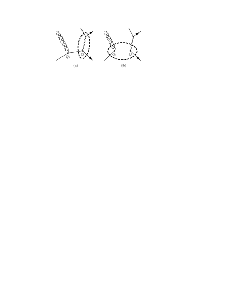
   Figure 2: Two possible cluster configurations of $W+1$ jet events. The dashed line highlights the hard $2\to 2$ process.

   The hard $2\to 2$ process either is again of the Drell–Yan type (Fig. 2a) or, for example, of the type $q\bar{q}^{\prime}\to gW$ (Fig. 2b). The respective weights in both cases read:

   $${\cal W}_{\rm ME}^{(a)} ={\cal W}_{\rm ME}^{(b)}=\Delta_{q}(Q,Q_{\rm cut})\,\Delta_{\bar{q}^{\prime}}(Q,Q_{\rm cut})\,\Delta_{g}(Q_{1},Q_{\rm cut})\frac{\alpha_{s}(Q_{1})}{\alpha_{s}(Q_{\rm cut})}\;.$$ (20)

   where $Q$ is the scale of the core $2\to 2$ process and the nodal value $Q_{1}$ is given by the transverse momentum of the extra jet. For the first configuration, $Q^{2}=p_{W}^{2}=M_{e\nu}^{2}$, and the gluon jet tends to be soft, i.e. $Q_{1}$ preferentially is close to $Q_{\rm cut}$. The second configuration differs from the first only by the result of the clustering and in the scale of the core process, now given by

   $$Q^{2}=p_{\perp,g}^{2}+M_{e\bar{\nu}_{e}}^{2}=M_{\perp,W}^{2}\,.$$ (21)

   The transverse momentum of the gluon jet $p_{\perp,g}^{2}$ now is of the order of the $W$-boson mass. In the first case, $Q_{1}=p_{\perp,g}$ emerges as a part of the clustering procedure, whereas in the second case, it is read off directly from the core process. It is important, however, that the scale in both cases is defined in the same way in order to guarantee a smooth transition between the regime where clustering (a) and the regime where clustering (b) is chosen.

   In both cases considered here, the parton shower for both the quark and the anti-quark in the initial state again starts with the respective scale $t$, and the parton distribution weights are treated in the same manner as before. The parton shower for the final state jet in contrast starts at $t_{1}$, all emissions in the three parton showers are vetoed if their transverse momentum exceeds $Q_{\rm cut}$.

3. $n=2$:
   Many processes contribute to the production of two extra jets, some illustrative examples are displayed in Fig. 3.

   

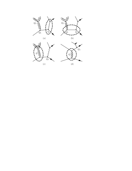
   Figure 3: Four possible cluster configurations of a W+2 jet event. The dashed line highlights the hard $2\to 2$ process, being either of Drell–Yan type (a), a vector boson production (b) or a pure QCD process (c,d).

   The cases a) and b) displayed there are very similar to the example with one extra jet only. The corresponding weights read:

   $${\cal W}_{\rm ME}^{(a)} ={\cal W}_{\rm ME}^{(b)}=\Delta_{q}(Q,Q_{\rm cut})\,\Delta_{\bar{q}^{\prime}}(Q,Q_{\rm cut})\,\Delta_{g}(Q_{1},Q_{\rm cut})\,\Delta_{g}(Q_{2},Q_{\rm cut})\frac{\alpha_{s}(Q_{1})}{\alpha_{s}(Q_{\rm cut})}\,\frac{\alpha_{s}(Q_{2})}{\alpha_{s}(Q_{\rm cut})}\;.$$ (22)

   The nodal value $Q_{2}$ is given by the $k_{\perp}$-algorithm, again it is the transverse momentum of the gluon. The scales $Q_{1}$ and $Q$ are chosen in full analogy to the one-jet case discussed above.

   In contrast a new situation arises when a pure QCD process has been chosen as the “core” $2\to 2$ process, see for instance Fig. 3c). Since the “core” process is not resolved, there is only one scale available, $Q^{2}=p_{\perp}^{2}$, the transverse momentum of the outgoing jets. The correction weight in this case thus reads:

   $${\cal W}_{\rm ME}^{(c)} =\Delta_{q}(Q,Q_{\rm cut})\,\frac{\Delta_{q}(Q,Q_{\rm cut})}{\Delta_{q}(Q_{1},Q_{\rm cut})}\,\Delta_{\bar{q}^{\prime}}(Q_{1},Q_{\rm cut})\,[\Delta_{g}(Q,Q_{\rm cut})]^{2}\left[\frac{\alpha_{s}(Q)}{\alpha_{s}(Q_{\rm cut})}\right]^{2}\,.$$ (23)

   In this case, the Sudakov form factors in the denominator corresponding to the internal quark line and its external continuation cancel only, if both quarks have the same mass, which is not necessarily the case.

   In contrast to the case exhibited in diagram 3c), where the boson was clustered with an initial state parton, Fig. 3d) pictures an example configuration, where the boson is clustered with a final state parton. In this case, the corresponding correction weight is given by

   $${\cal W}_{\rm ME}^{(d)} =[\Delta_{q}(Q,Q_{\rm cut})]^{2}\,\frac{\Delta_{q^{\prime}}(Q,Q_{\rm cut})}{\Delta_{q^{\prime}}(Q_{1},Q_{\rm cut})}\,\Delta_{q^{\prime\prime}}(Q_{1},Q_{\rm cut})\Delta_{\bar{q}^{\prime}}(Q,Q_{\rm cut})\left[\frac{\alpha_{s}(Q)}{\alpha_{s}(Q_{\rm cut})}\right]^{2}\,.$$ (24)

   The starting conditions for the parton showers for the first two cases, Fig. 3c) and 3b), are very similar to the $n=1$ case: The initial state partons start their evolution at $t$, the two extra jets start their evolution at $t_{1}$ and $t_{2}$, respectively, and all are subject to a jet veto inside the parton shower with transverse momentum $Q_{\rm cut}$. For the last two cases, the situation changes. There, the electroweak boson does not play any significant role for the parton shower; all four parton showers start at their common QCD core process scale, $t$. Of course, again, emissions with transverse momentum larger than $Q_{\rm cut}$ from any of the four shower seeds are vetoed. It should be noted here that there is a potential mismatch of logarithms of correction weight and veto weight in the quark line that changes its flavour. This happens if the two quarks adjacent to the electroweak boson have different mass; mass effects, however, usually can be safely neglected as long as no top quarks are present.

The extension to higher multiplicities is straightforward. However, assume again for illustrative reasons that $n_{\rm max}=2$, leading to the application of the highest multiplicity treatment for the two-jet configuration. Then, during cross section evaluation the factorisation scale is set dynamically to $\mu_{F}=Q_{s}$, i.e. to the nodal value of the softest emission. This leads to the following cross sections

$$\begin{array}[]{l@{\,=\,}r@{\extracolsep{15mm}} l@{\extracolsep{1mm}\,=\,}r@{\extracolsep{15mm}} l@{\extracolsep{0mm}\,\,}r}\sigma_{0}^{(0)}&953.03\mbox{\rm pb&\sigma_{0}^{\rm nmax=2}&825.77\mbox{\rm pb\\ \sigma_{1}^{(0)}&155.76\mbox{\rm pb&\sigma_{1}^{\rm nmax=2}&108.35\mbox{\rm pb\\ \sigma_{2}^{(0)}&34.29\mbox{\rm pb&\sigma_{2}^{\rm nmax=2}&22.01\mbox{\rm pb\\ \lx@intercol\hfil\hfil\lx@intercol&\sigma_{\rm tot}^{\rm nmax=2}&\lx@intercol\sum\limits_{i=0}^{2}\sigma_{i}^{\rm nmax=2}=956.13\mbox{\rm pb}\,.\hfil\lx@intercol\end{array}}}}}}}$$ (25)

Assuming that $Q_{2}<Q_{1}$, the correction weight for the diagram a) in Fig. 3 would read

$$\tilde{\cal W}_{\rm ME}^{(a)} =\Delta_{q}(Q,Q_{2})\,\Delta_{\bar{q}^{\prime}}(Q,Q_{2})\,\Delta_{g}(Q_{1},Q_{2})\,\Delta_{g}(Q_{2},Q_{2})\frac{\alpha_{s}(Q_{1})}{\alpha_{s}(Q_{2})}\,\frac{\alpha_{s}(Q_{2})}{\alpha_{s}(Q_{2})}$$

$$=\Delta_{q}(Q,Q_{2})\,\Delta_{\bar{q}^{\prime}}(Q,Q_{2})\,\Delta_{g}(Q_{1},Q_{2})\,\frac{\alpha_{s}(Q_{1})}{\alpha_{s}(Q_{2})}\;.$$ (26)

The parton showers for the four legs would start at $t$ for the two quark lines, and at $t_{1}$ and $t_{2}$ for the two gluon lines, respectively. Vetos would be applied for emissions with a $k_{\perp}$ larger than $Q_{2}$, which implies that there would be no jet veto in the parton shower evolution of the second gluon line. Of course, the scales in the parton distribution weights of the first initial state radiation inside the shower would also be adjusted.

The situation is even more extreme when considering diagram d). There, the softest QCD radiation actually is at the core process. Thus, no correction weight whatsoever would be applied, cf. Eq. 24, if the masses of $q^{\prime}$ and $q^{\prime\prime}$ are identical,

$$\tilde{\cal W}_{\rm ME}^{(d)} =[\Delta_{q}(Q,Q)]^{2}\,\frac{\Delta_{q^{\prime}}(Q,Q)}{\Delta_{q^{\prime}}(Q_{1},Q)}\,\Delta_{q^{\prime\prime}}(Q_{1},Q)\Delta_{\bar{q}^{\prime}}(Q,Q)\left[\frac{\alpha_{s}(Q)}{\alpha_{s}(Q)}\right]^{2}=\frac{\Delta_{q^{\prime\prime}}(Q_{1},Q)}{\Delta_{q^{\prime}}(Q_{1},Q)}\,.$$ (27)

All parton showers for all four legs would start at $t$, and the veto would be applied for emissions larger than $Q$, but this phase space region is kinematically excluded anyway.

3.3 Example III – $p\bar{p}\to\mbox{jets}$

In this example the operation of the multi-cut treatment is illustrated through the case of $p\bar{p}\to\leq 3\mbox{jets}$. The two-jet sample here is generated with a jet resolution cut of $Q_{\rm cut}^{(2)}=20$ GeV, and the three-jet sample is produced with $Q_{\rm cut}^{(3)}=30$ GeV. The corresponding a-priori cross sections read

$$\begin{array}[]{l@{\,=\,}r@{\extracolsep{15mm}} l@{\extracolsep{1mm}\,=\,}r@{\extracolsep{15mm}} ll}\sigma_{2}^{(0)}&30.423\mbox{\rm mb&\sigma_{2}^{\rm nmax=3}&13.903\mbox{\rm mb&\\ \sigma_{3}^{(0)}&0.133\mbox{\rm mb&\sigma_{3}^{\rm nmax=3}&0.092\mbox{\rm mb&\\ \lx@intercol\hfil\hfil\lx@intercol&\sigma_{\rm tot}^{\rm nmax=3}&\lx@intercol\sum\limits_{i=2}^{3}\sigma_{i}^{\rm nmax=3}=13.995\,\mbox{\rm mb}\hfil\lx@intercol\,.\end{array}}}}}$$ (28)

In their calculation, the factorisation scale of the two-jet events has consistently been set to $Q_{\rm min}$ defined as

$$Q_{\rm min}={\rm min}\left\{p_{\perp},Q_{\rm cut}^{(3)}\right\}\,,$$ (29)

where $p_{\perp}$ is the transverse momentum of the outgoing jets. In contrast, in the evaluation of the cross section of the three-jet events, the factorisation scale has consistently been set to $Q_{s}$, the scale of the softest jet.

Figure 4: Examples for the production two and three jets.

In Fig. 4, exemplary diagrams for the two processes, the production of two and three jets, are depicted. For a typical two jet event, such as the one in diagram a), the weight reads

$${\cal W}_{\rm ME}^{(a)} =[\Delta_{q}(Q,Q_{\rm min})]^{2}\,[\Delta_{g}(Q,Q_{\rm min})]^{2}\,\left[\frac{\alpha_{s}(Q_{\rm min})}{\alpha_{s}(Q_{\rm cut}^{(2)})}\right]^{2}\,.$$ (30)

The shower for all four legs starts at $t$, with a veto on emissions harder than $Q_{\rm min}$, and again the parton distribution weight in the first emission of each of the initial state shower evolutions is adjusted.

For the three-jet event depicted in diagram b), the weight reads

$${\cal W}_{\rm ME}^{(b)} =[\Delta_{q}(Q,Q_{s})]^{2}\,\Delta_{g}(Q,Q_{s})\frac{\Delta_{g}(Q,Q_{s})}{\Delta_{g}(Q_{1},Q_{s})}[\Delta_{q}(Q_{1},Q_{s})]^{2}\left[\frac{\alpha_{s}(Q)}{\alpha_{s}(Q_{\rm cut}^{(3)})}\right]^{2}\,\frac{\alpha_{s}(Q_{1})}{\alpha_{s}(Q_{\rm cut}^{(3)})}\,.$$ (31)

The parton shower for the two incoming quarks, for the outgoing gluon and for the harder of the two outgoing quarks starts at $t$, the parton shower of the softer of the two quarks emerging from the gluon line starts at $t_{1}$. The veto is performed w.r.t. the scale $Q_{1}$.

3.4 Example IV – $e^{+}e^{-}\to d\bar{d}u\bar{u}(g)$

In the process $e^{+}e^{-}\to d\bar{d}u\bar{u}$, there are basically three classes of subprocesses that can emerge as the core $2\to 2$ process, namely

• $e^{+}e^{-}\to W^{+}\,W^{-}$,

• $e^{+}e^{-}\to Z^{0}/\gamma\,Z^{0}/\gamma$, and

• $e^{+}e^{-}\to d\bar{d}$ or $e^{+}e^{-}\to u\bar{u}$ ,

all of which are depicted in Fig. 5. The first two are electroweak processes, with $W$ pair production usually largely dominating, whereas the latter can either lead to a QCD or to an electroweak topology. Interferences between QCD and electroweak diagrams are negligible, therefore it is convenient to consider both contributions as independent.

Figure 5: Possible cluster configurations in $e^{+}e^{-}\to d\bar{d}u\bar{u}(g)$. The dashed line indicates the core $2\to 2$ process.

In the following, the focus will be mainly on the electroweak contributions. There exist 4 different possibilities for the first clustering, listed in Tab. 1.

$i$&	$j$	Probability
$2$&	$4$	$P_{24}=p_{24}^{Z}+p_{24}^{\gamma}$
		$\displaystyle p_{24}^{Z}=\left[\frac{\alpha_{\rm QED}(\mu)}{\sin^{2}\theta_{w}}\right]^{2}\,\frac{(g_{1,d}^{2}+g_{2,d}^{2})(g_{1,e}^{2}+g_{2,e}^{2})}{(q^{2}-M_{Z}^{2})^{2}+M_{Z}^{2}\Gamma_{Z}^{2}}$
		$\displaystyle p_{24}^{\gamma}=[\alpha_{\rm QED}(\mu)]^{2}\,\frac{Q_{d}^{2}Q_{e}^{2}}{(q^{2})^{2}}$
$2$&	$5$	$P_{25}=p_{25}^{W}$
		$\displaystyle p_{25}^{W}=\left[\frac{\alpha_{\rm QED}(\mu)}{2\sin^{2}\theta_{w}}\right]^{2}\,\frac{(M^{\rm CKM}_{ud})^{2}}{(q^{2}-M_{W}^{2})^{2}+M_{W}^{2}\Gamma_{W}^{2}}$
$3$&	$4$	$P_{34}=p_{34}^{W}$
		$\displaystyle p_{34}^{W}=\left[\frac{\alpha_{\rm QED}(\mu)}{2\sin^{2}\theta_{w}}\right]^{2}\,\frac{(M^{\rm CKM}_{ud})^{2}}{(q^{2}-M_{W}^{2})^{2}+M_{W}^{2}\Gamma_{W}^{2}}$
$3$&	$5$	$P_{35}=p_{35}^{Z}+p_{35}^{\gamma}$
		$\displaystyle p_{35}^{Z}=\left[\frac{\alpha_{\rm QED}(\mu)}{\sin^{2}\theta_{w}}\right]^{2}\,\frac{(g_{1,u}^{2}+g_{2,u}^{2})(g_{1,e}^{2}+g_{2,e}^{2})}{(q^{2}-M_{Z}^{2})^{2}+M_{Z}^{2}\Gamma_{Z}^{2}}$
		$\displaystyle p_{35}^{\gamma}=[\alpha_{\rm QED}(\mu)]^{2}\,\frac{Q_{u}^{2}Q_{e}^{2}}{(q^{2})^{2}}$

Table 1: All possibilities for the (electroweak) first clustering of $e^{+}e^{-}\to d\bar{d}u\bar{u}$. For brevity of the example only one Feynman diagram is taken into account for each possible propagator flavour.

After, for instance, choosing $2$&$5$ (the $d\bar{u}$-pair) to be clustered first and to become a $W^{-}$ boson, a second clustering leads to the $2\to 2$ core process. Of course, the first step restricts the possibilities for any subsequent clustering - in this example three options remain. Their probabilities are listed Tab. 2.

$i$&	$j$	Probability
$2$&	$3$	$P_{23}=p_{23}^{d}$
		$\displaystyle p_{23}^{d}=\frac{1}{2}\left[\frac{\alpha_{\rm QED}(\mu)}{\sin^{2}\theta_{w}}\right]^{2}\,\frac{(M^{\rm CKM}_{ud})^{2}}{(q^{2})^{2}}(g_{1,u}^{2}+g_{2,u}^{2})$
$2$&	$4$	$P_{24}=p_{24}^{\bar{u}}$
		$\displaystyle p_{24}^{\bar{u}}=\frac{1}{2}\left[\frac{\alpha_{\rm QED}(\mu)}{\sin^{2}\theta_{w}}\right]^{2}\,\frac{(M^{\rm CKM}_{ud})^{2}}{(q^{2})^{2}}(g_{1,d}^{2}+g_{2,d}^{2})$
$3$&	$4$	$P_{34}=p_{34}^{W}$
		$\displaystyle p_{34}^{W}=\left[\frac{\alpha_{\rm QED}(\mu)}{2\sin^{2}\theta_{w}}\right]^{2}\,\frac{(M^{\rm CKM}_{ud})^{4}}{(q^{2}-M_{W}^{2})^{2}+M_{W}^{2}\Gamma_{W}^{2}}$

Table 2: All possibilities for the clustering of $e^{+}e^{-}\to W^{-}\bar{d}u$. For brevity of the example only one Feynman diagram is taken into account for each possible propagator flavour.

One possible outcome of the clustering procedure is a $W$ pair production process as depicted in Fig. 5a. The evaluation of the Sudakov weight in this case yields

$${\cal W}_{\rm ME}^{(a)} =\Delta_{d}(Q_{1},Q_{\rm cut})\Delta_{\bar{u}}(Q_{1},Q_{\rm cut})\Delta_{u}(Q_{2},Q_{\rm cut})\Delta_{\bar{d}}(Q_{2},Q_{\rm cut})$$ (32)

in the $WW$ case; when the $q\bar{q}$ production process is chosen instead, cf. Fig. 5b, the correction weight is given by

$${\cal W}_{\rm ME}^{(b)} =\Delta_{d}(Q_{1},Q_{\rm cut})\Delta_{\bar{u}}(Q_{1},Q_{\rm cut})\Delta_{u}(Q,Q_{\rm cut})\Delta_{\bar{d}}(Q,Q_{\rm cut})$$ (33)

Both weights look very similar, and indeed for massless quarks this holds true for all Sudakov weights that can be obtained. However, while in the first example both scales $Q_{1}$ and $Q_{2}$ are of the order $M_{W}$, the relevant scales in the second case are more likely to be $Q_{1}\approx M_{W}$ and $Q\approx 2M_{W}$, of course depending on the exact kinematical configuration. Of course, these different clusterings result in different starting conditions for the shower.

4 Results

The detailed presentation of examples in the previous section, Sec. 3 will be supplemented with results in this section. To validate the consistency of the approach, clearly a careful examination is mandatory, checking whether the exclusive samples prepared through the re-weighted matrix elements and further evolved through the parton shower combine into a consistent, inclusive sample. Any larger discontinuity that becomes visible, in particular on scales comparable to the merging scale $Q_{\rm cut}$, may serve as an indication for a mismatch of leading logarithms. Obviously, a good way of scrutinising the radiation pattern in the interaction of matrix elements and parton shower is to investigate differential jet rates, especially in a $k_{\perp}$ scheme. These rates are defined through the jet resolution in the corresponding scheme, where an $n+1$-jet event turns into an $n$-jet event.

4.1 Results for $e^{+}e^{-}\to\mbox{jets}$ at LEP I

To start with, differential jet rates in $e^{+}e^{-}\to\mbox{jets}$ are compared. In $e^{+}e^{-}$ annihilations, it is often convenient to define a variable $y_{\rm cut}$ rather than $Q_{\rm cut}$; in the Durham scheme employed here, it is defined through

$$y_{\rm cut} =\frac{Q_{\rm cut}^{2}}{E_{\rm c.m.}^{2}}$$ (34)

implying that two particles $i$ and $j$ belong to different jets if they are separated by a distance

$$y_{ij}\geq 2\frac{\mbox{\rm min}\{E_{i}^{2},E_{j}^{2}\}}{E_{\rm c.m.}^{2}}(1-\cos\theta_{ij})\,.$$ (35)

In Fig. 6, results for differential jet rates are shown ranging over four orders of magnitude in $y_{\rm cut}$. The dependence on the actual value of $Q_{\rm cut}$ in the generation of two different samples is barely visible. Also, the distributions seem to be perfectly smooth around the generation cut. Therefore, one may conclude that the merging in this case has been accomplished with very high quality.

Figure 6: Differential jet rates in the Durham scheme at LEP I. Shown are the results obtained through the merging of matrix elements for up to five jets with the parton shower, with two different separation cuts. The solid lines correspond to a cut at $y_{\rm cut}=10^{-2.5}$, and the dashed curve illustrates the result using $y_{\rm cut}=10^{-2}$. In the former case coloured lines indicate the contributions from individual matrix elements: two jets (red), three jets (green), four jets (blue), and five jets (purple).

The samples generated by SHERPA also reproduce event shape observables such as thrust, thrust-major, thrust-minor or oblateness, cf. Fig. 7. Again, the dependence on the generation cut is rather small, deviations are well below 20%.

Figure 7: Thrust (top left), thrust-major (top right), thrust minor (bottom left), and oblateness (bottom right) at LEP I. For definitions of these observables, cf. appendix LABEL:app:observables1. The hadron level result of SHERPA is pictured for two different separation cuts $y=10^{-2.5}$ and $y=10^{-2}$. Line styles and colours are the same as in Fig. LABEL:fig:lep_diffdurham1.

Going to more exclusive observables that are sensitive to the full interference structure of matrix elements, various four-jet correlations may be tested. Examples for such correlations are the Bengtsson-Zerwas and the Nachtmann-Reiter angle, see the appendix for their definition. In Fig. 8, data taken at LEP I [15] are compared with results of the merged samples of SHERPA and with a “shower”-only result. Of course, the latter lacks the exact treatment of quantum interferences, which is possible only through full matrix elements. Correspondingly, there is a visible shape difference between data and the merged sample on the one hand and the shower-only sample on the other hand. This beautifully underlines the power of the merging approach.

Figure 8: Four jet angle distributions. Shown are the Bengtsson-Zerwas angle (left) and the modified Nachtmann-Reiter angle (right). The data points are from a DELPHI measurement [15].

4.2 Results for $p\bar{p}\to W+\mbox{jets}$ at Tevatron, Run I

The investigations for the case of $p\bar{p}\to W+\mbox{jets}$ start with an analysis of differential jet rates in the $k_{\perp}$ algorithm for this process at Tevatron, Run I. Results of SHERPA with different jet resolution cuts during the generation of the respective sample are exhibited in Fig. 9. The results are not quite as good as those obtained for the previous case of $e^{+}e^{-}$ annihilations into jets, on the other hand, the example presented here is much more complicated. This extra complication is due to a more intricate radiation pattern with emissions in both the initial and the final state. Still the relative differences are marginal, ranging up to 20%. Only in the sample with the highest jet resolution cut it becomes apparent that the parton shower is not able to fill the phase space properly. This is the reason behind the visible hole in the differential jet rates around the cut.

Figure 9: Differential jet rates for the $1\to 0$, $2\to 1$ and $3\to 2$ transition (top to bottom), for $Q_{\rm cut}=10$ GeV, $30$ GeV, and $50$ GeV (from left to right). In each plot, the results are compared with those for $Q_{\rm cut}=20$ GeV.

In analogy to the event shapes above, the transverse momentum distribution of the $W$ boson and of the electron produced in its decay may be considered as inclusive observable. The dependence of these observables from the jet resolution cut in the generation of the samples and on the maximal number of jets covered by the matrix elements is displayed in Figs. 10 and 11, respectively. In both cases it becomes apparent that the dependences are negligible - results of different samples produced under different conditions are in very good agreement with each other.

Figure 10: $p_{\perp}(W^{-})$ and $p_{\perp}(e^{-})$ for $Q_{\rm cut}=10$ GeV, $30$ GeV and $50$ GeV in comparison with $Q_{\rm cut}=20$ GeV.

Figure 11: $p_{\perp}(W^{-})$ for $Q_{\rm cut}=15$ GeV and different maximal numbers of ME jets included. The dashed line corresponds to a maximal number of ME jets $n_{\rm max}=2$.

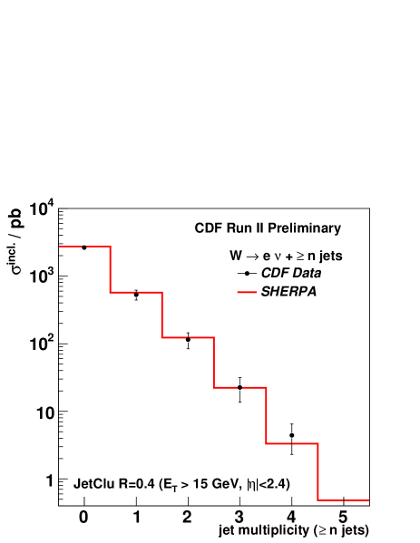
Figure 12: Inclusive cross sections for the process $p\bar{p}\to W+n$ jets. The SHERPA prediction is contrasted with the measurement by CDF [16]

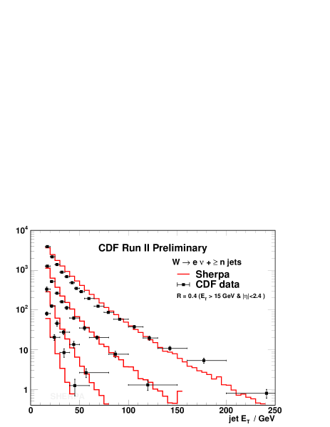
Figure 13: Jet transverse energy distribution for the process $p\bar{p}\to W+n$ jets from a CDF [16] measurement. Shown are the highest $E_{T}$ jet distribution in inclusive $W+1jet$ events, the second highest $E_{T}$ jet distribution in inclusive $W+2jet$ events, the third highest $E_{T}$ jet distribution in inclusive $W+3jet$ events, and the fourth highest $E_{T}$ jet distribution in inclusive $W+4jet$ events. The SHERPA result includes matrix elements with up to 4 jets.

Finally, measured total cross sections for different jet multiplicities in $W+{\rm jet}$ [16] are compared with those obtained from SHERPA after reweighting the matrix elements with up to 4 jets with the Sudakov weights and after applying a constant $K$-factor of $1.44$ to all samples, that has been calculated to match SHERPA with a NNLO prediction [17, 18]. Taking into account the errors, the results are in great agreement with each other, cf. Fig. 12. Correspondingly, the $p_{\perp}$ spectra of the jets are depicted in Fig. 13. There, the measurement of transverse energy distributions of jets for different multiplicities [16] are compared with results from SHERPA. Again, the results agree very well after applying a global $K$-factor on the latter. In both cases, jets were defined through a cone algorithm with cone size of $R=0.4$ and a transverse energy of the jets of at least $E_{T}=15$ GeV.

4.3 Results for $p\bar{p}\to\mbox{jets}$ at Tevatron, Run I

Before investigating in greater detail the consistency of the merging prescription for jet production at hadron colliders, in particular at the Tevatron, Run I, consider Fig. 14. There, the differential $3\to 2$ jet rates for samples with $n_{\rm max}=3$ for $Q_{\rm cut}=20$, $30$, and $40$ GeV are compared with a the result for a sample, where two different jet resolution cuts have been applied for the different multiplicities, namely $Q_{\rm cut}^{(2)}=30$ GeV and $Q_{\rm cut}^{(2)}=40$ GeV. Obviously, for $Q\geq 40$ GeV the four results are in fair agreement with each other, as expected. Below $40$ GeV, the sample generated with $Q_{\rm cut}=40$ GeV starts to undershoot the other three curves significantly, as expected. In principle, there should be no contribution left at all, since there are no matrix elements for any jet configurations populating this regime. However, due to the parton shower, some of the jets produced at higher $p_{\perp}$ values spread out, leading to some non-negligible fraction of events migrating into that region. The same pattern repeats itself at $Q$-values below $30$ GeV. This region is not filled by the $Q_{\rm cut}=30$ GeV and the mixed sample any longer. This implies that in order to describe jet observables at jet resolutions above, say, $30$ GeV, a $Q_{\rm cut}\leq 30$ GeV should be applied. Due to the steep descend of cross sections this may not be very efficient, rendering a multi-scale treatment the method of choice.

Figure 14: Differential $3\to 2$ jet rate at the Tevatron, Run I. Different samples with different values of $Q_{\rm cut}$ are displayed in different colours, the respective $Q_{\rm cut}$ values are indicated with dashed vertical lines. Clearly, above 40 GeV, all samples coincide, then successively, different samples die off. Apparently the sample with mixed cuts ($Q_{\rm cut}^{(2)}=30$ GeV and $Q_{\rm cut}^{(3)}=40$ GeV), depicted in purple, agress very well with the sample produced with the lower of the two cuts.

Figure 15: Differential $2\to 1$, $3\to 2$, $4\to 3$ jet rate at the Tevatron, Run I. The mixed sample with two cuts ($Q_{\rm cut}^{(2)}=30$ GeV and $Q_{\rm cut}^{(3)}=40$ GeV, as above), depicted with the solid black line is compared with a reference sample with one, common cut only ($Q_{\rm cut}^{(3)}=30$ GeV), displayed with the dashed black line. Deviations are maximally of the order of 20%, indicating the success of the multi-cut treatment. Note also that in the $3\to 2$ jet rate, around 40 GeV the effect of merging the 2 with the three jet configuration becomes visible.

In Fig. 15, the mixed sample from above is further investigated. There, in addition to the summed result, also the contributions from different jet multiplicities are displayed. Clearly, the two samples fill quite separate regions of phase space, i.e. above and below the jet resolution cut. Of course, as before, there is some residual migration of the samples over the respective jet resolution cut. The sum, however, is remarkably smooth over the cut. This allows to efficiently generate an inclusive QCD sample with jets resolved at $40$ GeV, for example, where higher jet configurations are accounted for by corresponding matrix elements and the phase space below the matrix element cuts for them is properly filled by the lowest multiplicity contribution. The quality of this approach is further highlighted in Figs. 16 and 17. There, again, differential jet rates are depicted, this time the cuts have been chosen as $Q_{\rm cut}^{(2)}=2.5$ GeV and $Q_{\rm cut}^{(\geq 3)}=10$ GeV. The plots cover up to ten orders of magnitude with an extremely smooth prediction.

Figure 16: Differential jet rates at the Tevatron, Run I. From left to right, the rates for $2\to 1$, $3\to 2$, and for $4\to 3$ transitions at the hadron level are exhibited; the samples are produced with $n_{\rm max}=3$ and $Q_{\rm cut}^{(2)}=2.5$ GeV & $Q_{\rm cut}^{(3)}=10$ GeV. A reference curve is shown in black-dashed lines, contributions from different multiplicities are displayed in different colours.

Figure 17: Differential jet rates at the Tevatron, Run I. From left to right, the rates for $2\to 1$, $3\to 2$, and for $4\to 3$ transitions at the hadron level are exhibited; the samples are produced with $n_{\rm max}=4$ and $Q_{\rm cut}^{(2)}=2.5$ GeV & $Q_{\rm cut}^{(3,4)}=10$ GeV. A reference curve is shown in black-dashed lines, contributions from different multiplicities are displayed in different colours.

4.4 Results for $e^{+}e^{-}\to d\bar{d}u\bar{u}(g)$ at LEP II

In this section, the quality of the alternative algorithm will be validated. To this end, $e^{+}e^{-}\to$jets at LEP II are chosen as the reference process.

4.4.1 QCD

Concentrating first on the case where QCD alone contributes to the production of extra jets, in Fig. 18 differential and total jet rates in the Durham scheme at LEP II as described with the original and with the alternative approach are compared. Clearly, the results are nearly indistinguishable. This implies that in this case the ordering of the hardness of emissions according to the $k_{\perp}$ measure is nearly identical with an ordering according to the virtual masses occurring in the propagator terms.

Figure 18: Differential (upper row) and total (lower row) jet rates in the Durham scheme at LEP II for QCD events. The result of the original and the alternative merging procedure are compared, (original=solid black, alternative=dashed red), differences are hardly visible.

The same holds also true for event shape observables, depicted in Fig. 19. There, measurements of thrust, thrust-major and the $C$-parameter [19] are exhibited and compared to the simulation of SHERPA. Again, the alternative and the original algorithm perform equally well and both reproduce nicely the data.

Figure 19: Thrust, thrust major and $C$-parameter. Delphi data [19] taken at LEP II events ($E_{\rm cms}=189$ GeV) are compared to simulation using the original and the alternative way of constructing the pseudo parton shower history (original=solid black, alternative=dashed red).

4.4.2 Electroweak interactions

It is expected that differences in the two prescriptions to reconstruct the pseudo parton shower history appear when the electroweak production of four quarks is investigated. Both for event shape observables displayed in Fig. 20 and for total or differential jet rates depicted in Fig. 21 the differences are sizable, reaching up to 50%.

Figure 20: Thrust, thrust-major and $C$-parameter in electroweak four jet events at LEP II. This time, the results of the two merging prescriptions (original=solid black, alternative=dashed red) differ significantly, by up to 50%.

Figure 21: Differential (upper row) and total (lower row) jet rates in electroweak four jet events at LEP II. The results of the two merging prescriptions (original=solid black, alternative=dashed red) are compared with each other, differences are visible.

This can be easily understood. In Fig. 22 the cross sections for three typical core $2\to 2$ processes are considered, namely $W$ pair production, $Z/\gamma$ pair production, and the QED/electroweak analogue to the QCD processes. Apparently, the alternative algorithm correctly reproduces the expected cross sections for the $WW$ and $ZZ$ channel (2 pb and 0.02 pb). Hence, the relative contributions of the three considered processes are consistent with the matrix element. In contrast, the original algorithm fails to reproduce the correct rate for the $WW$ channel, because it triggers an unphysical migration into the QCD-like configurations. Consequently, both samples differ in their colour structure, in their Sudakov weights and, ultimately, in the starting scales for their parton shower.

Figure 22: Statistics of selected “core” processes for different electroweak 4-jet channels. The result of the original (left plot) with the alternative algorithm (right plot) is compared.

This finding gives a clear hint that the pole structure of propagators has to be taken into proper account when merging such matrix elements with the parton shower. Thus, in the following, the focus will be on the self-consistency of such an approach. To investigate this, again differential and total jet rates are considered. In Fig. 24 corresponding results for a $4$ jet and for a combined $(4+5)$-jet sample produced according to the alternative algorithm are contrasted with each other. They are in nice agreement, hinting that the combination of exclusive samples into an inclusive one was successfully achieved. In Fig. 23 the corresponding event shape observables are shown. There, the differences between both samples are marginal; they differ only in the low-statistics bins. Note that in all Figs. 20-24 the multi-cut treatment has been employed. The 4-jet matrix element cut has been chosen to $y_{\rm cut}^{(4)}=10^{-4}$, while the 5-jet matrix element was separated by $y_{\rm cut}^{(5)}=10^{-2.2}$. This is important, since there exists no 3-jet matrix element, which could compensate for the phase space cut in the 4-jet matrix element.

Figure 23: Thrust, thrust-major and $C$-parameter in electroweak four jet events at LEP2. Results of SHERPA for a merged (4+5)-jet sample ($y_{\rm cut}=10^{-2.2}$) are contrasted with those of a pure 4-jet sample where the parton shower was running freely.

Figure 24: Differential (upper row) and total (lower row) jet-rates in electroweak four jet events at LEP2. Results of a merged (4+5)-jet sample ($y_{\rm cut}=10^{-2.2}$) are contrasted with those of a pure 4-jet sample.

5 Summary and Conclusion

In this publication, the procedure for a consistent merging of matrix elements for the production of multi-particle final states at tree-level and the parton shower has been discussed in great detail, going beyond the scope of previous publications on that subject. In particular, some improvements of the method have been presented which consistently treat situations, where the parton shower must fill the phase space for the production of jets which is not covered by corresponding matrix elements. In addition, some ideas of how to extent the original algorithm to cases were electroweak and strong interactions compete have been set forth. A large number of examples highlights how the algorithm works in various cases, results clearly demonstrate its ability to yield reliable and predictive results in $e^{+}e^{-}$ annihilations and in hadronic collisions.

Apart from the presentation of the method, its implementation into the new event generator SHERPA has been discussed. The relevant classes are described in sufficient detail to allow users of SHERPA to implement own ideas or to cross-check systematically the behaviour of the algorithm in cases not covered here.

Appendix A Brief program documentation

The module, in which the merging algorithm is implemented, is an integral part of the SHERPA framework. It is situated inside the main module SHERPA, and it employs SHERPAs basic physics tools, e.g., four-momenta, parton distribution functions, and jet algorithms. Of course, in its present form it has many connections to specific features of SHERPAs matrix element generator AMEGIC and its parton shower module APACIC. An extension to other matrix element generators or parton showers, however, is straightforward.

This section gives a brief overview over the classes responsible for the merging and their specific tasks within the algorithm. Where needed, details on specific implementation issues are presented that should, in principle, enable the interested user to implement and test some of his or her own ideas.

A.1 Implementation

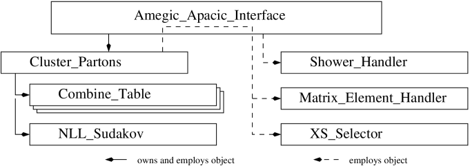
Figure 25: Ownership of the main classes responsible for the merging of ME and PS.

The basic algorithmic steps underlying the realisation of the merging algorithm in SHERPA can be summarised in the following way:

1. First of all, the pseudo parton shower history is reconstructed. To simplify the presentation, the focus here is on the implementation of the original approach only. Modifications to the extension described above can be found in the detailed description of the individual classes.

   • Take all Feynman diagrams with a binary tree structure, i.e. those that contain vertices with three legs only. For a given $2\to n$ process the resulting structure will have $n+2$ external particles. In AMEGIC, this doubly linked binary tree structure is represented through the class Point, each Point contains pointers to its predecessor and offsprings. In the merging procedure the Points of each Feynman diagram that correspond to an external particle are translated into a Leg. The merging is performed in terms of the Legs, which ensures that the underlying Feynman diagram structure is not modified through the algorithms.

   • Test all pairs of external particles, i.e. Legs. In the original version of the merging algorithm, for each allowed pair the relative transverse momentum according to the $k_{\perp}$ algorithm is calculated. Pairings which do not correspond to a junction in the Feynman diagrams, are discarded. Each allowed pairing is stored in a table, conveniently represented as a class Combine_Table, together with the list of diagrams where it occurs and with the $k_{\perp}$ value. Each Combine_Table has pointers to the previous one and its successor, i.e. to a Combine_Table with one Leg more, and to another one, with one Leg less.

   • In this Combine_Table the pairing with the smallest $k_{\perp}$ is selected. Their common predecessor is obtained from the first Feynman diagram(s) - in the original approach, the flavour of it is an unique choice anyhow. Its four-momentum is the sum of the two momenta of its offsprings, taken together this fully defines the intermediate particle, i.e. the corresponding Leg. It replaces the two offsprings and it is used for the next round of clustering, operating on a duly reduced number of Legs. All diagrams that did not contain the selected splitting are discarded in the further procedure.

   • The procedure terminates as soon as a splitting results in a structure with four external legs, i.e. a $2\to 2$ process.

2. The Sudakov weight for the selected configuration is evaluated.

   • The starting point is the core $2\to 2$ process. Its hard scale $Q_{h}$ is defined though the colour structure; in case there are different competing colour structures the winner is selected according to the relative weights. The details of this are implemented in an extra module of SHERPA, basically a library of $2\to 2$ processes called EXTRA_XS. It incorporates the processes as realisations of an abstract base class, XS_Base, the relevant one is chosen through an XS_Selector.

     In addition, the $2\to 2$ process determines the scale for the coupling weight, $Q_{\rm QCD}$. Then, however, this core process may result in a factor of

     $$\left[\alpha_{S}(Q_{\rm QCD})/\alpha_{S}(Q_{\rm cut})\right]^{m}\,,$$ (36)

     where $m$ is the number of strong interactions in the core process. In most cases, these two scales are identical, exceptions are, for instance, the process $e^{+}e^{-}\to q\bar{q}$, which for sure has no strong interaction, and therefore no scale $Q_{\rm QCD}$, cf. Sec. 2.

     At that point, each Leg is associated with a value $Q_{1}=Q_{h}$

   • The previous Combine_Table “unclusters” one of the particles and yields the corresponding nodal $k_{\perp}$ measure, $Q_{\rm 2}$. If the decay of this particle proceeds through the strong interaction, the weight is multiplied by

     $$\left[\alpha_{S}(Q_{2})/\alpha_{S}(Q_{\rm cut})\right]\,.$$ (37)

     If the decaying particle $a$ is strongly interacting, a Sudakov weight is attached, namely

     $$\left[\Delta_{a}(Q_{1},Q_{\rm cut})/\Delta_{a}(Q_{2},Q_{\rm cut})\right]\,,$$ (38)

     where $Q_{1}$ is the nodal value of the previous iteration step for this particle, i.e. the $k_{\perp}$ measure associated to the vertex, where it stems from. Then, for the two offsprings produced in the decay, their production scale is identified as $Q_{1}=Q_{2}$.

   • If no previous Combine_Table exists, there is no decaying particle left, and all Legs are external. Then, each Leg with strong quantum numbers results in a factor

     $$\Delta_{a}(Q_{1},Q_{\rm cut})$$ (39)

     attached to the Sudakov weight.

3. If the event is accepted after the Sudakov weight, the parton shower has to be attached. For this, the binary tree structure of the Points is translated to the Tree structure of APACIC. APACIC, however, does not order its shower in terms of transverse momenta. Instead it employs an ordering by virtuality. Therefore, for each particle, the virtual mass of its production vertex is identified and used as the starting scale of the parton shower evolution. Again, this is easily accomplished by just following the Combine_Table, starting from the core process.

A.2 Steering

The class Amegic_Apacic_Interface

is the central interface class, steering the various steps of the merging procedure. It is derived from the abstract class Perturbative_Interface. Each Perturbative_Interface owns pointers to a Shower_Handler and to a Matrix_Element_Handler, which provide access to the internal structure of the parton shower and to the matrix elements, respectively. In principle, other shower algorithms or another matrix element treatment can easily be connected to the SHERPA framework - from SHERPAs point of view merely the two handler classes (the Shower_Handler and the Matrix_Element_Handler) would have to be suitably extended, and a corresponding interface of the type ME_PS_Interface would have to be constructed.

The Amegic_Apacic_Interface is used through consecutive calls to the following methods.

• DefineInitialConditions()
  performs all steps necessary in order to construct a pseudo parton shower history and its corresponding weight, to accept or reject this configuration, and, eventually, to initialise the parton shower. In particular for the first task, it heavily relies on the helper class Cluster_Partons, presented below. Depending on the success of the procedure, the integer return value of this method is “0”, “1” or “3” indicating a rejected event, an accepted event, or a rejected event after the lose-jet-veto, respectively.

  DefineInitialConditions() executes the following steps:

  1. Cluster the matrix element configuration to a $2\to 2$ core process by calling ClusterConfiguration().

  2. Determine the starting scale and colour connections of this core process with the help of an XS_Base from the EXTRA_XS library. The corresponding process is selected through a call of Cluster_Partons::GetXS().

  3. Evaluate the NLL Sudakov weight used for reweighting the ME kinematics through Cluster_Partons::CalculateWeight(). Accept or reject the configuration accordingly.

  4. If accepted initialise the parton shower evolution by employing Cluster_Partons::FillTrees().

• ClusterConfiguration()
  is used to obtain a pseudo parton shower history. The clustering actually is achieved in the helper class, through the method Cluster_Partons::ClusterConfiguration(). This method merely forms an intelligent wrapper around it, and it prepares merging Blobs of the type ”ME PS Interface”. These Blobs are used to translate the on-shell partons from the matrix element into the off-shell partons experiencing the parton shower. Therefore they are filled after the parton shower evolution. The latter is triggered by

• PerformShowers(),
  which calls the appropriate routine in the Shower_Hander. The jet-veto scale and the renormalisation scale, which have been determined in the merging procedure before, are handed over to the parton shower, also through the Shower_Hander. If the shower evolution was successful,

• FillBlobs()
  inserts the prepared and filled “ME PS Interface” and the shower Blobs into the event record.

Apart from ClusterConfiguration(), which is obsolete for instance for $2\to 2$ processes, these general methods have to be provided by any realisation of a Perturbative_Interface.

The class Cluster_Partons

is the class central to the implementation of the merging algorithm. It has three main routines, and a number of helper methods, which will be discussed in the following:

• ClusterConfiguration()
  is the method that clusters a given $2\to n$ process until a $2\to 2$ core process remains. In so doing, it creates a history of successive emissions, each of which is associated with a specific emission scale, the nodal value of the respective clustering. The algorithm for the clustering implemented here proceeds as follows:

  1. All possible Feynman graphs are iterated over. In AMEGIC, a diagram consists of a doubly linked tree of Points. They represent vertices, whereas the links are the propagating particles. Also, the external particles of each diagram are represented as Points, but with all but one of the links empty. The number of diagrams and these Point structures themselves are accessible through the methods Matrix_Element_Handler::NumberOfDiagrams() and Matrix_Element_Handler::GetDiagram(), respectively. However, the external particles of each diagram, both incoming and outgoing are translated into Legs, on which the actual clustering is performed without disturbing the Points underneath.

  2. These first Legs and their four-momenta are stored in a Combine_Table. Ultimately, it is this class, which, step by step, clusters two particles, i.e. Legs into an intermediate particle, i.e. Leg. Its four-momentum in due course will be given by the appropriate combination of the two incident particles. As a result of this particular step, a new Combine_Table emerges with the number of Legs diminished by one, which is linked to the previous one.

     Having thus filled the first Combine_Table through its method FillTable, the list of all emerging Combine_Tables is constructed by calling CalcJet() of the fist one.

• GetXS()
  identifies the hard $2\to 2$ core process. In particular, it determines the colour structure of it, and the relevant hard scale(s). The preferred way to carry out this task is to employ an internal library of analytical $2\to 2$ processes provided by the module EXTRA_XS. An implemented cross section calculator can be obtained by XS_Selector::GetXS(), selecting the process in question through the flavours of its external particles. The cross section calculator is realised as an XS_Base, and it has suitable routines available for selecting colour connections (XS_Base::SetColours()) and for retrieving a renormalisation scale (XS_Base::Scale()).

  An alternative solution exists for those processes which are not implemented yet but for which the colour connections are unambiguously defined. This is actually always the case if the number of strongly interacting particle involved is smaller than four. Then, the colour connections are explicitely constructed, using the routine Cluster_Partons::SetColours(). In this case the hard scale reads

  $$Q_{\rm hard}^{2} =\left\{\begin{array}[c]{lll}p_{\perp}^{2}+p_{3}^{2}+p_{4}^{2}&\mbox{if initial and final state are colour connected, and}\\[5.69054pt] (p_{1}+p_{2})^{2}&\parbox{227.62204pt}{if there is no colour connection between \\ initial and final state,}\end{array}\right.$$ (42)

  with $p_{1}$/$p_{2}$ and $p_{3}$/$p_{4}$ denoting the four-momenta of the incoming and outgoing particles, respectively. In case there are 3 coloured particles involved in the hard process, a scale for the evaluation of the strong coupling has to be determined too, which is identified with the transverse momentum $p_{\perp}$ of the outgoing coloured particle.

• CalculateWeight()
  follows the previously obtained history and calculates from it the corresponding Sudakov weight according to the merging prescription described above. For this, the nodal values $Q_{i}$ determined before in ClusterConfiguration() are employed. The start scale for the Sudakov weight $Q_{h}$ and the scale $Q_{\rm QCD}$ for possible $\alpha_{S}$ factors have been prepared by GetXS()/SetColours(), see above.

  The construction of the weight starts with the core $2\to 2$ process. Hence, the first part of the weight is given by a factor $({\alpha_{S}(Q_{\rm QCD})}/{\alpha_{S}(Q_{\rm cut})})^{m}$, with $m$ specifying the number of strong couplings involved in the hard process. The clustering is followed backward through the sequence of Combine_Tables, adding a factor

  $$w =\frac{\Delta(Q_{i},Q_{\rm cut})}{\Delta(Q_{j},Q_{\rm cut})}\frac{\alpha_{S}(Q_{j})}{\alpha_{S}(Q_{\rm cut})}\,,$$ (43)

  for each internal line constructed during the backward clustering. The Sudakov form factors $\Delta(Q_{i},Q_{\rm cut})$ are provided by the method Delta() of the class NLL_Sudakov. The algorithm ends with a factor as $\Delta(Q_{i},Q_{\rm cut})$ for any dangling coloured particle, with possible another coupling weight in case of the extended merging algorithm (see Sec. 2).

• FillTrees()
  translates the pseudo parton shower history into the Tree structures, which APACIC uses to represent the parton shower. This history includes the starting scales of the shower evolution of each parton and possible constraints on shower emissions such as, e.g., opening angles determined from colour connections of the partons. The Knots forming the Tree are taken from the pseudo parton shower through Point2Knot(), the mutual relations are constructed through EstablishRelations().

• EstablishRelations()
  builds a tree by creating mutual links between a given set of three Knots. At each step, the actual Tree represents a partially performed shower. For the mutual relations, three cases are distinguished

  1. two incoming partons from the hard $2\to 2$ process:
     the energy fractions $x_{1}$ and $x_{2}$ are filled from the information in the Combine_Table.

  2. two outgoing partons from a common mother:
     The two final state particles are initialised using Final_State_Shower::EstablishRelations(). There, the more energetic parton is initialised with the angle and virtuality of the mother, the less energetic parton is initialised with angle and virtuality of the current branch.

  3. one incoming parton, its mother and its sister:
     The incoming parton, its mother and its sister are initialised using Initial_State_Shower::SetColours(). Note, angle conditions inside the shower are fixed only during shower evolution. The starting scale of the shower is given by the virtual mass of the mother due to APACICs shower evolution in terms of virtualities.

• DetermineColourAngles()
  determines the maximum angle between colour connected partons of a hard $2\to 2$ process. These angles are used in the explicit angular vetoes of the parton shower.

  For initial state particles the colour angle is determined in the lab frame after a boost along the $z$-axis, whereas starting angles for the final state system are determined in its c.m. frame. The starting angles are stored in the variable “thcrit” of each knot.

A number of simple access methods make the result of the clustering process available to the interface class Amegic_Apacic_Interface.

• Weight() returns the weight calculated in CalculateWeight().

• Scale() returns the hardest scale (of the core process) as determined in SetColours().

• AsScale() returns the scale associated with the strong coupling in the core process as determined in SetColours().

• Flav() provides the flavours of the core $2\to 2$ process.

• Momentum() returns the momenta of the core $2\to 2$ process.

A.3 Clustering

The class Combine_Table

provides the structure for storing histories of successive clusterings. The structure fills itself recursively, with the only input being the Feynman diagrams of the process under consideration and the four-momenta of the current event.

Each Combine_Table consists of a list of possible clusterings (particles $i$, $j$ and the flavour of the resulting intermediate particle) and the $k_{\perp}$ values and Feynman diagrams associated with them. These informations are realised through the classes Combine_Key and Combine_Data, see below. In addition, a number of methods allows a Combine_Table to create these data and to construct the sequence of Combine_Tables representing the clustering history:

• FillTable()
  has two tasks to fulfil. First of all, a set of given Legs, i.e. particles, are filled into the table. Then, all pairs of them are checked whether they can be clustered. A clustering is possible only, if it occurs in a corresponding Feynman diagram, which disables unphysical parton histories. This check is performed through the method Combinable(), see below.

• CalcJet()
  evaluates the $k_{\perp}$ distance of all allowed parton pairs ($i$,$j$) created by FillTable() with the Jet_Finder. After that, a pair to be clustered is selected according to the merging prescription, and a new Combine_Table is constructed, where the number of Legs is reduced by one. Consequently, after each clustering step, the set of Feynman diagrams is pruned, to include only those where the selected combination is possible. The four-momentum of the new (joined) Leg is given by the corresponding combination of the two individual four momenta. The algorithm continues recursively with corresponding calls to FillTable() and CalcJet() until only a $2\to 2$ process remains.

• CalcPropagator()
  performs all basic calculations for the determination of cluster probability for a given pair ($i$,$j$). This usually includes the evaluation of the $k_{\perp}$ measure, and the invariant mass $s_{ij}$. In case of the extended clustering algorithm, an estimate for the branching probability is also computed, which includes the couplings of that branching process, as well as the corresponding propagator. The couplings are available in the Feynman diagrams provided by AMEGIC.

• Combinable
  determines whether two particles, i.e. Legs can be clustered. To this end, the two Points related to the Legs are checked whether they have a common third Point, i.e. vertex, linked to them.

To exemplify the description above, consider the representation of a Combine_Table below.

$i$&	$j$	$y_{ij}$	$graphs$	$down$ link to the next table
0&	2	0.0810366	2,3,4,5,8
0&	4	0.0691623	6,7	$\to$ Combine_Table 2
1&	3	0.0844243	0,1,6,7,8
1&	4	0.293399	4,5
2&	4	0.111385	0,1
3&	4	0.215127	2,3

For each combination ($i$,$j$) a $k_{\perp}$ measure $y_{ij}$ and a list of contributing Feynman $graphs$ is stored. For the winner combination a $down$ link to a subsequent Combine_Table is provided. In addition the Combine_Table contains a list of four-momenta of the current configuration, and a matrix of all dangling legs (one row for each graph), as well as a reference to the winner combination ($i$,$j$), and an $up$-link to the table with one combination less performed.

In case the extended merging algorithm is applied, the Combine_Table also has to include further information needed for the winner determination: the virtuality of the resulting propagator $s_{ij}$, the estimate of the propagator $prop$, and the $coupling$ of the corresponding vertices.

The class Leg

represents a particle dangling from a Feynman diagram. It stores all information of a AMEGIC::Point and an extra ”anti”-flag.

Since AMEGIC::Point is the basic component of a Feynman graph representation in AMEGIC, it can be conveniently used in the clustering process to determine possible combinations and resulting propagators. The additional $anti$-flag helps to keep track of charge conjugations during the clustering process. In order to access all information of a Point more easily the operator-> is overloaded.

The class Combine_Key

is one of the basic elements for the creation of a Combine_Table. It includes the numbers of combinable legs ($i$ and $j$) and the flavour of the resulting propagator. It is used as a key in a fast access map in Combine_Table in order to access the information placed in a Combine_Data object.

The class Combine_Data

is the basic element for the determination of clustering when using a Combine_Table. It includes the distance of two legs $i$ and $j$ according to a $k_{\perp}$ measure ($y_{ij}$), a list of numbers of graphs where this combination is possible ($graphs$) and a link to the new table where those legs have been combined ($down$).

In case the extended merging algorithm is active, additional information is included, namely: the virtuality of the resulting propagator $s_{ij}$, the estimate of the propagator $prop$, and the $coupling$ of the corresponding vertices.

A.4 Weighting

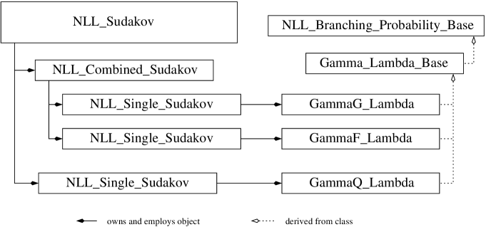
Figure 26: Ownership and inheritance diagram of the main classes related to the numerical evaluation of NLL Sudakov form factors. The sketch corresponds to the status after the initialisation via NLL_Sudakov::PrepareMap().

The class NLL_Sudakov

provides the numerical values for the Sudakov form factors used in the merging procedure of parton shower and matrix elements. Consequently, the main routine is Delta(const ATOOLS::Flavour &), which returns the Sudakov form factor for a given flavour. A corresponding table of Sudakov form factor objects for all possible flavours is created by respective calls to PrepareMap() or PrepareMassiveMap().

In the following a short description of the individual methods of this class is given.

• Delta (const ATOOLS::Flavour &)
  is the main access method to NLL Sudakov form factors. It returns the appropriate NLL Sudakov form factor (in form of a NLL_Sudakov_Base object) for any given flavour. For not strongly interacting particles a reference to a NLL_Dummy_Sudakov object is provided.

  For instance, a typical call to determine the numerical value of the gluon Sudakov form factor at a scale $Q$ with a jet resolution scale $Q_{0}$ would look like

        double  dg = sud.Delta(Flavour(kf::gluon))(Q,Q0);
  

• PrepareMap()
  initialises a map with all massless Sudakov form factors needed in the Standard Model. In so doing, a Sudakov form factor (cf. NLL_Single_Sudakov and NLL_Combined_Sudakov) is initialised for each strongly interacting flavour (d-, u-, s-, c-, b-quark or anti-quark, and gluon) and put into a map for fast access. For the sake of completeness, a NLL_Dummy_Sudakov (always one) is added to the map, which will be returned for any flavour without a dedicated Sudakov form factor. The default massless integrated splitting functions used for the evaluation of the Sudakov form factors are GammaQ_Lambda, GammaG_Lambda, and GammaF_Lambda.

• PrepareMassiveMap()
  initialises a map with all massive Sudakov form factors. This method is very similar to PrepareMap(). However, using the massive version of Sudakov form factors necessitates the initialisation of a NLL_Single_Sudakov for each flavour (d-, u-, s-, c-, b-quark) individually being now distinguishable by their mass (cf. [20, 21]). The default massive integrated splitting functions used are GammaQ_Lambda_Massive, GammaG_Lambda_Massive, and GammaF_Lambda_Massive. An overview of the implemented branching probabilities is given in Tab. 3.

The class NLL_Sudakov_Base

is a pure virtual base class, providing an interface to any Sudakov form factor like object.

The class NLL_Single_Sudakov

provides the Sudakov form factor for a single given integrated splitting function.

The class NLL_Combined_Sudakov

provides the Sudakov form factor for a sum of integrated splitting functions.

The class NLL_Dummy_Sudakov

is a simple example of an Sudakov returning always one. It can be used for only weakly interacting flavours.

The class NLL_Branching_Probability_Base

represents a prototype for a branching probability (integrated splitting function), which can be used in the evaluation of Sudakov form factors (cf. class NLL_Sudakov). All realisations are derived from this class. A list of available branching probabilities can be found in Tab. 3. In general single integrated splitting functions have the form

$$\Gamma(Q,q)=\int_{z-(q/Q)}^{z+(q/Q)}dz\frac{\alpha_{S}(q)}{\pi}P(z)\,,$$

where $\alpha_{S}$ is the (running) strong coupling and $P(z)$ is the splitting kernel.

The class provides methods to access the branching probability $\Gamma(Q,q)$ through Gamma($q$,$Q$) as well as the value of the integrated branching probability

$$-\log(\Delta(Q,Q_{0}))=\int_{Q_{0}}^{Q}\,dq\,\Gamma(Q,q)\,.$$

The latter is accessible through IntGamma($Q_{0}$,$Q$), which is used as the basis of Sudakov form factors.

$$\alpha_{\mbox{\tiny S}}^{\mu}(Q) =\frac{\alpha_{\mbox{\tiny S}}(\mu)}{1-\displaystyle\frac{\beta_{0}}{4\pi}\frac{\alpha_{\mbox{\tiny S}}(\mu)}{\log(\mu^{2}/Q^{2})}} \eta_{0} =\frac{\beta_{0}\alpha_{\mbox{\tiny S}}(\mu)}{4\pi}\log\left(\frac{Q_{0}^{2}}{\mu^{2}}\right) \eta_{1} =\frac{\beta_{0}\alpha_{\mbox{\tiny S}}(\mu)}{4\pi}\log\left(\frac{Q^{2}}{\mu^{2}}\right)$$

$$\alpha_{\mbox{\tiny S}}^{\Lambda}(Q) =\frac{2\pi}{\beta_{0}\log(Q/\Lambda)} \xi_{0} =\log\frac{Q_{0}}{\Lambda} \xi_{1} =\log\frac{Q}{\Lambda}$$

Table 3: Available implementations of NLL branching probabilities.

Appendix B Observables

The global properties of hadronic events may be characterised by a set of observables, usually called event shapes. In section 4 the following shape observables have been considered.

• Thrust $T$ :
  The thrust axis $\vec{n}_{T}$ maximises the following quantity

  $$T=\max_{\vec{n}_{T}}\left(\frac{\sum_{i}|\vec{p}_{i}\cdot\vec{n}_{T}|}{\sum_{i}|\vec{p}_{i}|}\right)\,,$$ (44)

  where the sum extends over all particles in the event. The thrust $T$ tends to 1 for events that has two thin back-to-back jets (“pencil-like” event), and it tends towards $1/2$ for perfectly isotropic events.

• Thrust Major $T_{\rm Major}$ :
  The thrust major vector $\vec{n}_{\rm Major}$ is defined in the same way as the thrust vector, but with the additional condition that $\vec{n}_{\rm Major}$ must lie in the plane perpendicular to $\vec{n}_{T}$:

  $$T_{\rm Major}=\max_{\vec{n}_{\rm Major}\perp\vec{n}_{T}}\left(\frac{\sum_{i}|\vec{p}_{i}\cdot\vec{n}_{\rm Major}|}{\sum_{i}|\vec{p}_{i}|}\right)\,.$$ (45)

• Thrust Minor $T_{\rm Minor}$ :
  The minor axis is perpendicular to both the thrust axis and the major axis, $\vec{n}_{\rm Minor}=\vec{n}_{T}\times\vec{n}_{\rm Major}$. The value of thrust minor is then given by

  $$T_{\rm Minor}=\frac{\sum_{i}|\vec{p}_{i}\cdot\vec{n}_{\rm Minor}|}{\sum_{i}|\vec{p}_{i}|}\,.$$ (46)

• Oblateness $O$ :
  The oblateness is defined as the difference between thrust major $T_{\rm Major}$ and thrust minor $T_{\rm Minor}$ :

  $$O=T_{\rm Major}-T_{\rm Minor}$$ (47)

• C-parameter $C$ :
  The C-parameter is derived from the eigenvalues of the linearised momentum tensor $\Theta^{\alpha\beta}$ , defined by

  $$\Theta^{\alpha\beta}=\frac{1}{\sum_{i}|\vec{p}_{i}|}\sum_{i}\frac{p_{i}^{\alpha}p_{i}^{\beta}}{|\vec{p}_{i}|}\,,\;\alpha,\beta=\{x,y,z\}\;.$$ (48)

  The three eigenvalues $\lambda_{i}$ of this tensor define $C$ with

  $$C=3\,(\lambda_{1}\lambda_{2}+\lambda_{2}\lambda_{3}+\lambda_{1}\lambda_{3})\,.$$ (49)

References

- [1] S. Catani, F. Krauss, R. Kuhn and B. R. Webber, JHEP 0111 (2001) 063 [arXiv:hep-ph/0109231].
- [2] F. Krauss, JHEP 0208 (2002) 015 [arXiv:hep-ph/0205283].
- [3] S. Catani, Y. L. Dokshitzer, M. Olsson, G. Turnock and B. R. Webber, Phys. Lett. B 269 (1991) 432.
- [4] S. Catani, Y. L. Dokshitzer and B. R. Webber, Phys. Lett. B 285 (1992) 291.
- [5] S. Catani, Y. L. Dokshitzer, M. H. Seymour and B. R. Webber, Nucl. Phys. B 406 (1993) 187.
- [6] T. Gleisberg, S. Höche, F. Krauss, A. Schälicke, S. Schumann and J. C. Winter, JHEP 0402 (2004) 056 [arXiv:hep-ph/0311263].
- [7] L. Lönnblad, Acta Phys. Polon. B 33, 3171 (2002).
- [8] L. Lönnblad, Comput. Phys. Commun. 71, 15 (1992).
- [9] M. L. Mangano, M. Moretti and R. Pittau, Nucl. Phys. B 632 (2002) 343 [arXiv:hep-ph/0108069].
- [10] R. Kuhn, F. Krauss, B. Ivanyi and G. Soff, Comput. Phys. Commun. 134 (2001) 223 [arXiv:hep-ph/0004270].
- [11] S. Mrenna and P. Richardson, JHEP 0405 (2004) 040 [arXiv:hep-ph/0312274].
- [12] F. Krauss, A. Schälicke, S. Schumann and G. Soff, Phys. Rev. D 70 (2004) 114009 [arXiv:hep-ph/0409106].
- [13] F. Krauss, A. Schälicke, S. Schumann and G. Soff, [arXiv:hep-ph/0503280].
- [14] T. Gleisberg, F. Krauss, A. Schälicke, S. Schumann and J. Winter, in preparation.
- [15] H. Hoeth, Diploma Thesis, Fachbereich Physik, Bergische Universität Wuppertal, 2003 [WUD 03-11].
- [16] G. Hesketh [D0 & CDF Collaboration], arXiv:hep-ex/0405067. see also Andrea Messina, in preparation.
- [17] R. Hamberg, W. L. van Neerven and T. Matsuura, Nucl. Phys. B 359 (1991) 343 [Erratum, ibid. B 644 (2002) 403].
- [18] R. V. Harlander and W. B. Kilgore, Phys. Rev. Lett. 88 (2002) 201801 [arXiv:hep-ph/0201206].
- [19] J. Abdallah et al. [DELPHI Collaboration], Eur. Phys. J. C 29 (2003) 285 [arXiv:hep-ex/0307048].
- [20] F. Krauss and G. Rodrigo, arXiv:hep-ph/0303038.
- [21] G. Rodrigo, M. S. Bilenky and A. Santamaria, Nucl. Phys. B 554 (1999) 257 [arXiv:hep-ph/9905276].