Abstract

This thesis is devoted to properties of quark matter at high density and (comparatively) low temperature. In nature matter under these conditions can possibly be found in the interior of (some) neutron stars. Under “normal” conditions quarks are confined in the hadrons. Under the extreme conditions in the core of a neutron star, however, the strong interaction between the quarks becomes weaker because of asymptotic freedom. Then the hadrons will break up, and for the remaining interaction between the quarks a (semi-)perturbative treatment should be sufficient, at least at asymptotic densities.

It turns out that cold dense quark matter does not behave like a Fermi liquid as a consequence of long-range chromomagnetic interactions between the quarks. While the specific heat of a Fermi liquid is a linear function of the temperature ($T$) at low temperature, the specific heat of normal (non-superconducting) quark matter is proportional to $T\log T$ at low temperature. In this thesis the specific heat and the quark self energy in normal quark matter are discussed in detail. A discrepancy between earlier papers on the specific heat is resolved by showing that in one of these papers gluonic contributions to the energy density were overlooked. Moreover higher order corrections to the known leading order terms are computed in this thesis in a systematic manner.

The quark-quark interaction mediated by one-gluon exchange is attractive in the color antitriplet channel. Therefore quarks form Cooper pairs at sufficiently small temperatures, which leads to the phenomenon of color superconductivity. During the last years the issue of gauge (in)dependence of the color superconductivity gap has been discussed in the literature. Here a formal proof is given that the fermionic quasiparticle dispersion relations in a color superconductor are gauge independent. In a color superconductor the gluon field acquires a non-vanishing expectation value in general, which acts as an effective chemical potential for the color charge. This expectation value is computed for two different color superconducting phases (2SC and CFL). It is shown that at leading order this expectation value is determined from a tadpole diagram with a quark loop. Tadpole diagrams with gluon or Nambu-Goldstone loops turn out to be negligible at our order of accuracy.

meinen Eltern gewidmet

Chapter 1 Introduction

We know four fundamental interactions in nature, namely gravitational, electromagnetic, weak and strong interactions. Since this thesis is devoted to properties of quark matter, we shall mainly be concerned with the strong interactions. Today the accepted theory of strong interactions is Quantum Chromodynamics (QCD). It is a gauge theory with gauge group $SU(3)_{c}$, where the index $c$ stands for color. The quarks belong to the fundamental representation of this group, and the gauge bosons (gluons) belong to the adjoint representation. Denoting the quark field with $\psi$ and the gluon field with $A$, one writes the Lagrangian of QCD as [1, 2]

$$\mathcal{L}_{QCD}=-{1\over 4}F_{\mu\nu}^{a}F^{a\mu\nu}+\sum_{f=1}^{N_{f}}\bar{\psi}_{i,f}\left(i\not{D}_{ij}-m_{f}\delta_{ij}\right)\psi_{i,f},$$ (1.1)

with $\not{D}=\gamma^{\mu}D_{\mu}$, $F_{\mu\nu}^{a}=\partial_{\mu}A_{\nu}^{a}-\partial_{\nu}A^{a}_{\mu}-gf^{abc}A_{\mu}^{b}A_{\nu}^{c},$ and $D_{\mu,ij}=\partial_{\mu}\delta_{ij}+igA_{\mu}^{a}T^{a}_{ij}.$ In Eq. (1.1) we have written explicitly the sum over quark flavors. Apart from the invariance under $SU(3)_{c}$ gauge transformations, the Lagrangian (1.1) is also invariant under global unitary transformations in flavor space as long as the differences of the quark masses can be neglected. In the chiral limit ($m_{f}\to 0$) the Lagrangian is even invariant under separate flavor space transformations of left and right handed quarks, with the corresponding symmetry groups $SU(N_{f})_{L}$ and $SU(N_{f})_{R}$. Moreover the Lagrangian (1.1) is invariant under global $U(1)$ phase transformations of the quark fields, which is related to quark number conservation.

The quantum theory based on the Lagrangian (1.1) is renormalizable [4, 5, 6]. Neglecting the quark masses for the moment, one finds for the one-loop beta function

$$\beta(g)=-{g^{3}\over 16\pi^{2}}\left(11-{\textstyle{2\over 3}}N_{f}\right).$$ (1.2)

Nature chooses $N_{f}=6$. (For many physical situations the number of “active” flavors is smaller than six. E.g. for the astrophysical systems, on which we eventually focus, we need to take into account only the three lightest flavors.) Therefore the beta function is negative, which shows that QCD possesses the all-important property of asymptotic freedom [8, 9].

Experimental confirmations of QCD come from deep inelastic scattering experiments, and other high energy processes (see [10] and references therein). These experiments give a current world average of [10]

$$\alpha_{s}(M_{Z})=0.1187\pm 0.002$$ (1.3)

with $\alpha_{s}={g^{2}\over 4\pi}$, and $M_{Z}=91.1876\pm 0.0021\,\mathrm{GeV}$ is the mass of the $Z$ boson.

At small energies quarks and gluons are confined into hadrons. In the confined phase chiral symmetry is spontaneously broken by a non-vanishing quark condensate $\langle\bar{q}q\rangle$, with $\pi$, $K$ and $\eta$ playing the role of (pseudo-)Nambu-Goldstone bosons. The low-energy dynamics of the hadrons can be described with chiral perturbation theory [11, 12].

From asymptotic freedom one expects at sufficiently high temperatures a phase transition to a deconfined phase [13]. The resulting “soup” of quarks and gluons is called quark gluon plasma (QGP). This idea is corroborated by lattice simulations, which predict a phase transition at $T_{c}\sim 170\,\mathrm{MeV}$ for $N_{f}=2$ [14, 15], and at $T_{c}\sim 150\,\mathrm{MeV}$ for $N_{f}=3$ [15]. It is assumed that the QGP existed in the early universe. Experimentalists try to reproduce the QGP in heavy ion collisions at SPS (CERN), at RHIC (Brookhaven), and from 2007 onwards at LHC (CERN).

The equation of state (the pressure as a function of the temperature) of the high temperature QGP has been computed perturbatively up to order $g^{6}\log g$ (see [16] and references therein). The expansion in the coupling constant turns out to be only poorly convergent for non-asymptotic temperatures. It is however possible to improve the situation by performing systematic resummations of the perturbative series, such as resummations within dimensional reduction [16, 19], HTL-screened perturbation theory [20, 21], or approximately selfconsistent resummations based on the 2PI effective action, [22, 23, 24] which show good agreement with the lattice data for $T\gtrsim 2T_{c}$. For reviews on the high temperature QGP see e. g. [25, 26, 27, 28, 29, 30].

It is of great importance to understand the properties of the quark gluon plasma also at finite chemical potential. This region of the QCD phase diagram is relevant for the interior of compact stars [31, 32, 33]. From asymptotic freedom one expects a phase transition to a deconfined phase to occur not only at high temperature, but also at high density. Unfortunately one does not know an efficient algorithm for lattice simulations at finite $\mu$. The reason is that the fermion determinant in the path integral is complex at finite $\mu$, which precludes Monte Carlo importance sampling. So far this “sign problem” can only be circumvented for $\mu<T$ (see [28] and references therein). But for the region $\mu\gg T$, which is relevant for compact stars, no method of implementing lattice simulations is known to date. Therefore simplified models, such as Nambu-Jona-Lasinio models [34, 35, 36], and (semi-)perturbative methods are the only viable approaches at the moment. In compact stars the chemical potential might be as large as $500\,\mathrm{MeV}$. At this energy scale $\alpha_{s}(\mu)$ is of the order one, therefore the applicability of (semi-)perturbative methods is rather questionable. Nevertheless one can try to extrapolate results which have been obtained for small values of the coupling constant to larger values of the coupling constant, hoping that the qualitative features remain valid.

Compared to the chemical potential, the temperature in the interior of a compact star will be rather small (of the order of tens of $\mathrm{keV}$ [32]). In this region of the QCD phase diagram quark matter is expected to be in a color superconducting phase, which is characterized by a non-vanishing diquark condensate. Such diquark condensates can arise from the fact that one gluon exchange is attractive in the color antitriplet channel, leading to the formation of Cooper pairs at sufficiently small temperatures. Color superconductivity has been discussed already in the late 1970’s [37, 38], but at that time it was believed that the color superconductivity gap would be of the order $1\,\mathrm{MeV}$, and thus almost negligible. Only some years ago [39, 40] it was realized that the gap may be as large as $\sim 10-100\,\mathrm{MeV}$, with corresponding critical temperatures of the order $\sim 5-50\,\mathrm{MeV}$. This discovery stimulated extensive research in this field during the last few years, see e.g. [41, 42, 43, 44, 45, 46, 47, 48] for reviews.

Due to the interplay of finite quark masses and the constraints from color and electric neutrality, there may be various color superconducting phases in the QCD phase diagram, which are distinguished mainly by the particular form of the diquark condensate. These matters will be reviewed in more detail in chapter 5 of this thesis.

In nature color superconducting phases could in principle be discovered from analyses of neutron star data. There exist indeed some proposals for signatures that could indicate the presence of color superconductivity. For instance, the cooling behavior of a neutron star depends on the specific heat and the neutrino emissivity, which are both sensitive to the phase structure (see e.g. [49, 50, 51, 52, 53]). Other possible signatures include $r$-mode instabilities [54, 55], and pulsar glitches due to crystalline structures in inhomogeneous color superconducting phases [56].

This thesis is organized as follows. In chapter 2 we discuss some formal properties of gauge theories, which will be used in chapter 5. In chapters 3 and 4 we compute the quark self energy and the specific heat of normal degenerate quark matter. These results may be relevant for the cooling properties of (proto-) neutron stars [57]. Chapter 5 is devoted to color superconductivity. We give a general proof that the fermionic quasiparticle dispersion relations in a color superconductor are gauge independent. Furthermore we compute gluon tadpole diagrams, which are related to color neutrality. Chapter 6 finally contains our conclusions.

Throughout this thesis we shall use the following conventions. We use natural units, $\hbar=c=k_{B}=1$. The Minkowski metric is $g^{\mu\nu}=\mathrm{diag}(1,-1,-1,-1)$. Four momenta are denoted as $K^{\mu}=(k_{0},{\bf k})$. The absolute value of the three momentum is denoted as $k:=|{\bf k}|$. A unit three vector is denoted as ${\bf\hat{k}}:={\bf k}/k$.

Chapter 2 Symmetries in quantum field theory

2.1 General gauge dependence identities

In this section we will recapitulate the derivation of a general gauge dependence identity, following [58, 59, 60].

Let us consider an arbitrary gauge theory which is defined by an action functional $S_{inv}[\varphi]$ that is invariant under some gauge transformations,

$$\delta\varphi^{i}=D^{i}_{\alpha}[\varphi]\delta\xi^{\alpha}.$$ (2.1)

Here we use the DeWitt notation [61], where an index $i$ comprises all discrete and continuous field labels, and a Greek index ($\alpha$) comprises group and space-time indices. E.g. for QCD, as defined by the Lagrangian (1.1), one has explicitly [with $\alpha\leftrightarrow(x,a)$]

$$\begin{array}[]{rll}D^{i}_{\alpha}\to&(\delta^{ab}\partial_{\mu}^{y}-gf^{abc}A_{\mu}^{c}(y))\delta(x-y),&\quad i\leftrightarrow A_{\mu}^{b}(y),\vspace{1.5mm}\\ &-igT^{a}\psi(y)\,\delta(x-y),&\quad i\leftrightarrow\psi(y),\vspace{1.5mm}\\ &ig\bar{\psi}(y)T^{a}\,\delta(x-y),&\quad i\leftrightarrow\bar{\psi}(y).\end{array}$$ (2.2)

In general we assume that the gauge generators form an off-shell closed algebra, which means that the commutator of two gauge transformations is again a gauge transformation,

$$D^{i}_{\alpha,j}[\varphi]D^{j}_{\beta}[\varphi]-D^{i}_{\beta,j}[\varphi]D^{j}_{\alpha}[\varphi]=c^{\gamma}_{\alpha\beta}[\varphi]D^{i}_{\gamma}[\varphi],$$ (2.3)

where the “structure constants” $c^{\gamma}_{\alpha\beta}$ can in principle be field dependent.

In order to quantize the theory we have to fix the gauge freedom, e.g. with a quadratic gauge fixing term,

$$S_{inv}[\varphi]\to S_{gf}[\varphi]=S_{inv}[\varphi]+{1\over 2}F^{\alpha}[\varphi]F_{\alpha}[\varphi].$$ (2.4)

The quantum theory is defined via the path integral representation of the generating functional of connected Green’s functions,

$$\exp(iW[J])=\int{\mathcal{D}}\varphi\det\left(F^{\alpha}_{,i}[\varphi]D^{i}_{\beta}[\varphi]\right)\exp\left(i\left(S_{gf}[\varphi]+J_{i}\varphi^{i}\right)\right).$$ (2.5)

With the help of a Legendre transformation

$$W[J]=\Gamma[\bar{\varphi}]+J_{i}\bar{\varphi}^{i},\qquad\bar{\varphi}^{i}:={\delta W[J]\over\delta J_{i}},$$ (2.6)

one obtains the effective action,

$$\exp(i\Gamma[\bar{\varphi}])=\int{\mathcal{D}}\varphi\det\left(F^{\alpha}_{,i}[\varphi]D^{i}_{\beta}[\varphi]\right)\exp\left(i\left(S_{gf}[\varphi]-\Gamma_{,i}[\bar{\varphi}](\varphi-\bar{\varphi})^{i}\right)\right).$$ (2.7)

If a change $\delta F^{\alpha}[\varphi]$ in the gauge fixing condition is accompanied by the following (non-local) gauge transformation,

$$\delta\varphi^{i}=D^{i}_{\alpha}[\varphi]\delta\Xi^{\alpha}[\varphi],\quad\delta\Xi^{\alpha}[\varphi]=\mathcal{G}^{\alpha}_{\ \beta}[\varphi]\delta F^{\beta}[\varphi],$$ (2.8)

the gauge fixed action $S_{gf}$ will remain invariant. Here $\mathcal{G}^{\alpha}_{\ \beta}$ is the ghost propagator in a background field $\varphi$, which is defined via

$$\left(F^{\alpha}_{,i}D^{i}_{\beta}\right)[\varphi]\mathcal{G}^{\beta}_{\ \gamma}[\varphi]=-\delta^{\alpha}_{\gamma}.$$ (2.9)

Let us examine in which way the measure and the Faddeev Popov determinant change under the gauge transformation (2.8) and $\delta F^{\alpha}$. From the measure we get a Jacobian, which can be evaluated for small $\delta\varphi^{i}$ using the formula

$$\det({\bf 1}+\mathcal{X})\simeq 1+\mathrm{Tr}\mathcal{X},$$ (2.10)

which is valid if $|\mathcal{X}_{ij}|\ll 1$. The variation of the Faddeev Popov determinant can be calculated using Eq. (C.1). In this way we find

$$\!\!\!\!\!\!\!\!\!\!\!\!\!\delta\left(\mathcal{D}\varphi\det\left(F^{\alpha}_{,i}D^{i}_{\beta}\right)[\varphi]\right)=\mathcal{D}\varphi\det\left(F^{\alpha}_{,i}D^{i}_{\beta}\right)\left[\mathrm{Tr}{\delta(\delta\varphi)^{i}\over\delta\varphi^{j}}+\delta\mathrm{Tr}\log\left(F^{\alpha}_{,i}D^{i}_{\beta}\right)\right]$$

$$\!\!\!\!\!=\mathcal{D}\varphi\det\left(F^{\alpha}_{,i}D^{i}_{\beta}\right)\left[D^{i}_{\alpha,i}\mathcal{G}^{\alpha}_{\ \beta}\delta F^{\beta}+\mathcal{G}^{\alpha}_{\ \beta}F^{\beta}_{,i}\left(D^{j}_{\alpha}D^{i}_{\gamma,j}-D^{j}_{\gamma}D^{i}_{\alpha,j}\right)\mathcal{G}^{\gamma}_{\ \delta}\delta F^{\delta}\right].\qquad$$ (2.11)

The first term between the brackets in the second line vanishes if $D^{i}_{\alpha,i}=0$. Using Eqs. (2.3) and (2.9) one finds that the remaining part vanishes provided that $c^{\beta}_{\beta\alpha}=0$. These two conditions are fulfilled for QCD, and also for the Higgs models which we will discuss in this chapter.

The only term in Eq. (2.7) which is not invariant is the source term $\Gamma_{,i}[\bar{\varphi}]\varphi^{i}$. Therefore we find the following gauge dependence identity,

$$\delta\Gamma[\bar{\varphi}]=-\Gamma_{,i}[\bar{\varphi}]\langle D^{i}_{\alpha}[\varphi]\mathcal{G}^{\alpha}_{\ \beta}[\varphi]\delta F^{\beta}[\varphi]\rangle[\bar{\varphi}]=:\Gamma_{,i}[\bar{\varphi}]\delta X^{i}[\bar{\varphi}],$$ (2.12)

where we use the notation

$$\!\!\!\!\!\!\!\!\!\!\!\!\!\!\!\langle K[\varphi]\rangle[\bar{\varphi}]$$

$$\!\!\!\!\!\!\!\!\!\!\!\!=e^{-i\Gamma[\bar{\varphi}]}\int\mathcal{D}\varphi\,K[\varphi]\det\left(F^{\alpha}_{,i}[\varphi]D^{i}_{\beta}[\varphi]\right)\exp\left(i\left(S_{gf}[\varphi]-\Gamma_{,i}[\bar{\varphi}](\varphi-\bar{\varphi})^{i}\right)\right)\qquad$$ (2.13)

for any $K[\varphi]$.

As an application let us consider the effective potential $V_{eff}$ for a translationally invariant system,

$$\Gamma[\bar{\varphi}]|_{\bar{\varphi}=\mathrm{const.}}=-V_{eff}(\bar{\varphi})\int d^{4}x.$$ (2.14)

In general $V_{eff}$ will be a gauge dependent quantity. However, the identity (2.12) ensures that

$$\delta V_{eff}(\bar{\varphi})+\delta X^{i}[\bar{\varphi}]{\partial V_{eff}(\bar{\varphi})\over\partial\bar{\varphi}^{i}}=0.$$ (2.15)

This is the Nielsen identity for the effective potential [59, 62], which states that a change in the gauge fixing function (the first term on the left hand side) can be compensated by a change in $\bar{\varphi}$ (the second term on the left hand side). This identity implies that the value of the effective potential at its minimum (where $\partial V_{eff}/\partial\bar{\varphi}^{i}=0$) is gauge independent.

A further consequence of the identity (2.12) is the gauge independence of the position of the propagator singularities [60, 62, 63, 64], which we will discuss in more detail in the sections 2.3 and 2.4 and in chapter 5.

2.2 Implications of global symmetries

The aim of this section is to examine the consequences of global symmetries for the one-point and two-point functions in quantum field theory.

Let us consider an arbitrary quantum field theory with field content $\Phi^{i}(x)$, $\bar{\Phi}^{i}(x)$. We assume that the theory is invariant with respect to a group $G$ of continuous global symmetry transformations, which act on the fields as

$$\Phi_{i}^{\prime}(x)=g_{ij}\Phi_{j}(x),\quad\bar{\Phi}_{i}^{\prime}(x)=\bar{\Phi}_{j}(x)g_{ji}^{\dagger},$$ (2.16)

where the $g_{ij}$ form some representation of $G$. The effective action up to second order can be written as

$$\Gamma[\Phi]\simeq\int d^{4}x\,\Gamma_{i}(x)\Phi_{i}(x)+\int d^{4}x\,\bar{\Gamma}_{i}(x)\bar{\Phi}_{i}(x)$$

$$\quad\qquad+\int d^{4}x\,d^{4}y\,\Gamma_{ij}(x,y)\Phi_{i}(x)\bar{\Phi}_{j}(y)+\mathcal{O}(\Phi^{3}).$$ (2.17)

We assume that the symmetry is not (spontaneously) broken. Then we have $\Gamma[\Phi]=\Gamma[\Phi^{\prime}],$ which implies

$$\Gamma_{i}(x)=g_{ji}\Gamma_{j}(x),$$ (2.18)

$$\bar{\Gamma}_{i}(x)=\bar{\Gamma}_{j}(x)g_{ij}^{\dagger},$$ (2.19)

$$\Gamma_{ij}(x,y)=g_{ki}\Gamma_{kl}(x,y)g_{jl}^{\dagger},$$ (2.20)

for all $g$. First let us consider Eqs. (2.18) and (2.19). With the additional assumption that the representation formed by the set of all $g$’s is non-trivial and irreducible, these equations imply that

$$\Gamma_{i}(x)=0,\quad\bar{\Gamma}_{i}(x)=0.$$ (2.21)

which means that the tadpole diagrams vanish (in other words, the expectation values of the field operators are zero).

If we assume that the representation is unitary, we can write Eq. (2.20) as

$$\Gamma^{T}_{ji}(x,y)=g_{jl}^{-1}\Gamma^{T}_{lk}(x,y)g_{ki}.$$ (2.22)

If we assume furthermore that the representation is irreducible, we can now invoke Schur’s lemma, which gives the result

$$\Gamma_{ij}\propto\delta_{ij},$$ (2.23)

i.e. the (inverse) propagator is proportional to the unit matrix with respect to the group indices.

Next we would like to examine in which way parity ($P$) and time reversal symmetry ($T$) constrain the propagator. For simplicity we work in Euclidean space and assume that our fields $\phi^{i}$ transform under $PT$ as

$$\phi^{i}(x)\rightarrow c^{(i)}\phi^{i}(-x),$$ (2.24)

with $c^{(i)}=\pm 1$. [This comprises for instance vector fields and (pseudo-)scalar fields.] Assuming translational invariance, the bilinear part of the effective action can be written as

$$\Gamma_{2}[\phi]={1\over 2}\int{d^{4}K\over(2\pi)^{4}}\phi^{i}(-K)\Gamma_{ij}(K)\phi^{j}(K),$$ (2.25)

where $\Gamma_{ij}$ is the full inverse propagator. Invariance under $PT$ implies

$$\Gamma_{2}[\phi]={1\over 2}c^{(i)}c^{(j)}\int{d^{4}K\over(2\pi)^{4}}\phi^{i}(K)\Gamma_{ij}(K)\phi^{j}(-K).$$ (2.26)

Performing the substitution $K\rightarrow-K$ in the last equation and comparing it with Eq. (2.25) we find $\Gamma_{ij}(K)=c^{(i)}c^{(j)}\Gamma_{ij}(-K).$ The mere definition of the inverse propagator implies $\Gamma_{ij}(K)=\Gamma_{ji}(-K)$, and therefore we have

$$\Gamma_{ij}(K)=c^{(i)}c^{(j)}\Gamma_{ji}(K).$$ (2.27)

Using Dyson’s equation

$$\Delta^{ij}\Gamma_{jk}=-\delta^{i}_{k}$$ (2.28)

we arrive at the following identity for the full propagator,

$$S^{ij}(K)=c^{(i)}c^{(j)}S^{ji}(K).$$ (2.29)

For $c^{(i)}c^{(j)}=1$ the propagator is therefore symmetric in $i$ and $j$.

2.3 Abelian Higgs model

This and the next section serve as an illustration of the application of the gauge dependence identities for systems with spontaneous symmetry breaking at finite temperature. We will discuss the gauge independence of the locations of propagator singularities, both for the Abelian and a non-Abelian Higgs model. This is actually more than a simple exercise, since the methods that we develop here will be useful also in the more complicated context of color superconductivity, which will be the subject of the last chapter of this thesis.

Let us also mention that the static limit of the gauged Higgs model yields the Landau-Ginzburg Lagrangian, which can be used for instance for the description of superconducting systems in the vicinity of the transition temperature [38]. In this thesis, however, we shall not go into the details of the Landau-Ginzburg description of superconducting systems.

There exists a vast literature on various aspects of Higgs models, let us just mention Refs. [65, 66, 67, 68, 69, 70, 71, 72], in which the finite temperature behavior of Higgs models is discussed.

2.3.1 Definition of the model

The Abelian Higgs is defined by the Lagrangian

$$\mathcal{L}_{inv}=-{1\over 4}F_{\mu\nu}F^{\mu\nu}+(D_{\mu}\Phi)(D^{\mu}\Phi)^{*}-V(\Phi)$$ (2.30)

with $F_{\mu\nu}=\partial_{\mu}A_{\nu}-\partial_{\nu}A_{\mu}$, $D_{\mu}=\partial_{\mu}+ieA_{\mu}$, $\Phi={1\over\sqrt{2}}(\varphi_{1}+i\varphi_{2})$, and

$$V(\Phi)=m^{2}\Phi^{*}\Phi+{\lambda\over 3!}(\Phi^{*}\Phi)^{2}.$$ (2.31)

The Lagrangian (2.30) is invariant under the gauge transformation

$$\delta\Phi=i\alpha\Phi,\quad\delta A_{\mu}=-{1\over e}\partial_{\mu}\alpha.$$ (2.32)

We assume $m^{2}<0$ so that the gauge symmetry is spontaneously broken. The expectation value of $\Phi$ is taken to be real so that $\varphi_{1}$ is the Higgs boson and $\varphi_{2}$ is the would-be Nambu-Goldstone boson. $\mathcal{L}_{inv}$ is invariant with respect to a ${\mathbbm{Z}}_{2}$ symmetry [59]:

$$A_{\mu}\rightarrow-A_{\mu},\qquad\varphi_{2}\rightarrow-\varphi_{2}$$ (2.33)

Following [59] we choose a gauge fixing which does not break the ${\mathbbm{Z}}_{2}$ symmetry:

$$\mathcal{L}_{gf}={1\over 2\alpha}(f\cdot A+\kappa\varphi_{2})^{2}$$ (2.34)

with some constant $\kappa$ and $f_{\mu}=\partial_{\mu}$, $f_{\mu}=(0,\partial_{i})$ or $f_{\mu}=u_{\mu}$, where $u_{\mu}=(1,0,0,0)$. In momentum space we write $\tilde{f}_{\mu}=\beta(K)K_{\mu}+\gamma(K)\tilde{n}_{\mu}$ with $\tilde{n}^{\mu}=(g^{\mu\nu}-K^{\mu}K^{\nu}/K^{2})u_{\nu}$. If $f_{\mu}=u_{\mu}$ we will assume $\kappa=0$ because otherwise time reversal symmetry would be violated. The corresponding ghost Lagrangian is given by

$$\mathcal{L}_{ghost}=\bar{c}\left(-{1\over e}f\cdot\partial+2\alpha\kappa\varphi_{1}\right)c.$$ (2.35)

The total Lagrangian

$$\mathcal{L}=\mathcal{L}_{inv}+\mathcal{L}_{gf}+\mathcal{L}_{ghost}$$ (2.36)

is still invariant under (2.33), which implies that Green functions (derivatives of the effective action, $\Gamma_{,ijk\ldots}|_{A=\varphi_{2}=0,\varphi_{1}=\bar{\varphi}}$) with an odd total number of external $A$- and $\varphi_{2}$-legs will vanish. Using Dyson’s equation (2.28) is is easy to see that this is also true for general Green functions.

2.3.2 Free propagators

The free propagators can be obtained easily by evaluating the path integral for the free theory. One finds that the free propagators are simply given by inverting the “coefficients” of the kinetic (bilinear) terms in the Lagrangian. If $\phi_{i}(x)$ is the solution of the free field equation,

$${\delta S_{bil.}\over\delta\phi_{i}(x)}=J_{i}(x),$$ (2.37)

one finds for the free propagator

$$G_{ij}(x,y)={\delta\phi_{j}(y)\over\delta J_{i}(x)}.$$ (2.38)

In this way one obtains the following tree level propagators for the Abelian Higgs model (with the notation “5”=$\varphi_{2}$):

$$\Delta_{(0)}^{\mu\nu} = {1\over K^{2}-e^{2}\bar{\varphi}_{(0)}^{2}}\Big{(}\mathcal{A}^{\mu\nu}+\mathcal{B}^{\mu\nu}-{\gamma k\over\beta K^{2}-e\kappa\bar{\varphi}_{(0)}^{2}}\mathcal{C}^{\mu\nu}$$ (2.39)

$$-{\gamma^{2}k^{2}+(\alpha K^{2}+\kappa^{2})(K^{2}-e^{2}\bar{\varphi}_{(0)}^{2})\over(\beta K^{2}-e\kappa\bar{\varphi}_{(0)})^{2}}\mathcal{D}^{\mu\nu}\Big{)},$$

$$\Delta_{(0)}^{\mu 5} = {ik\over K^{2}(K^{2}-e^{2}\bar{\varphi}_{(0)}^{2})(\beta K^{2}-e\kappa\bar{\varphi}_{(0)})^{2}}$$ (2.40)

$$\times\Big{[}\left(-e\gamma^{2}k^{2}\bar{\varphi}_{(0)}-K^{2}(\beta\kappa+\alpha e\bar{\varphi}_{(0)})(K^{2}-e^{2}\bar{\varphi}_{(0)}^{2})\right)\mathcal{E}^{\mu}\qquad$$

$$+{\gamma k\over\alpha}\left(2\beta^{2}K^{2}\kappa+\alpha\beta eK^{2}\bar{\varphi}_{(0)}+\alpha e^{2}\kappa\bar{\varphi}_{(0)}\right)\mathcal{F}^{\mu}\Big{]},$$

$$\Delta_{(0)}^{55} = -{e^{2}\gamma^{2}k^{2}\bar{\varphi}_{(0)}^{2}+K^{2}(K^{2}-e^{2}\bar{\varphi}_{(0)}^{2})(\beta^{2}K^{2}+\alpha e^{2}\bar{\varphi}_{(0)}^{2})\over K^{2}(K^{2}-e^{2}\bar{\varphi}_{(0)}^{2})(\beta K^{2}-e\kappa\bar{\varphi}_{(0)})^{2}},$$ (2.41)

$$\Delta_{(0)}^{\varphi_{1}\varphi_{1}} = -{1\over K^{2}-m^{2}-{\lambda\over 2}\bar{\varphi}_{(0)}^{2}},$$ (2.42)

where

$$\mathcal{A}^{\mu\nu}=g^{\mu\nu}-{K^{\mu}K^{\nu}\over K^{2}}-{\tilde{n}^{\mu}\tilde{n}^{\nu}\over\tilde{n}^{2}},\quad\mathcal{B}^{\mu\nu}={\tilde{n}^{\mu}\tilde{n}^{\nu}\over\tilde{n}^{2}},$$ (2.43)

$$\mathcal{C}^{\mu\nu}={1\over k}(\tilde{n}^{\mu}K^{\nu}+K^{\mu}\tilde{n}^{\nu}),\quad\mathcal{D}^{\mu\nu}={K^{\mu}K^{\nu}\over K^{2}},$$ (2.44)

$$\mathcal{E}^{\mu}={K^{\mu}\over k},\quad\mathcal{F}^{\mu}={\tilde{n}^{\mu}\over\tilde{n}^{2}},$$ (2.45)

and $\bar{\varphi}_{(0)}$ is the position of the minimum of the tree level potential, i.e.

$$\bar{\varphi}_{(0)}=\sqrt{-6m^{2}\over\lambda}.$$ (2.46)

We notice that all the structure functions are gauge dependent at tree level apart from $\Delta_{A(0)}$, $\Delta_{B(0)}$ and $\Delta^{\varphi_{1}\varphi_{1}}_{(0)}$.

The (full) propagators have the following symmetries: the definition of propagators implies $\Delta^{ij}=\Delta^{ji}$, and therefore in the non-condensed notation

$$\Delta^{\mu\nu}(K)=\Delta^{\nu\mu}(-K),\quad\Delta^{\mu 5}(K)=\Delta^{5\mu}(-K).$$ (2.47)

Invariance with respect to parity and time reversal implies (see Sec. 2.2)

$$\Delta^{\mu\nu}(K)=\Delta^{\mu\nu}(-K),\quad\Delta^{\mu 5}(K)=-\Delta^{\mu 5}(-K).$$ (2.48)

Eqs. (2.47) and (2.48) yield

$$\Delta^{\mu\nu}(K)=\Delta^{\nu\mu}(K),\quad\Delta^{\mu 5}(K)=-\Delta^{5\mu}(K).$$ (2.49)

If one used the gauge condition (2.34) with $f_{\mu}=u_{\mu}$ and $\kappa\neq 0$, (2.48) and (2.49) would not be valid, and an explicit calculation shows that a term which is antisymmetric in $\mu\nu$ would indeed appear already in the tree level propagator $\Delta_{(0)}^{\mu\nu}$.
We may parametrize the full propagators as follows:

$$\Delta^{\mu\nu} = \Delta_{A}\mathcal{A}^{\mu\nu}+\Delta_{B}\mathcal{B}^{\mu\nu}+\Delta_{C}\mathcal{C}^{\mu\nu}+\Delta_{D}\mathcal{D}^{\mu\nu},$$ (2.50)

$$\Delta^{\mu 5} = \Delta_{1}\mathcal{E}^{\mu}+\Delta_{2}\mathcal{F}^{\mu},$$ (2.51)

We perform an analogous decomposition for the two-point functions $\Gamma_{\mu\nu}$ and $\Gamma_{\mu 5}$ which are obtained from the effective action. These are one-particle irreducible apart from possible tadpole insertions. We also define self energies in the usual manner as $\Pi_{ij}=\Delta_{(0)ij}^{-1}-\Delta_{ij}^{-1}$.

With the help of Dyson’s equation (2.28) one can express the structure functions of the full propagators in terms of the self energies in the following way:

$$\Delta_{A} = -{1\over\Gamma_{A}},$$ (2.52)

$$\Delta_{B} = {\Gamma_{1}^{2}-\Gamma_{55}\Gamma_{D}\tilde{n}^{2}\over-\Gamma_{1}^{2}\Gamma_{B}+2\Gamma_{1}\Gamma_{2}\Gamma_{C}+\Gamma_{2}^{2}\Gamma_{D}+\Gamma_{55}(\Gamma_{C}^{2}+\Gamma_{B}\Gamma_{D})\tilde{n}^{2}},$$ (2.53)

$$\Delta_{C} = {\Gamma_{1}\Gamma_{2}+\Gamma_{55}\Gamma_{C}\tilde{n}^{2}\over\Gamma_{1}^{2}-\Gamma_{55}\Gamma_{D}\tilde{n}^{2}}\Delta_{B},$$ (2.54)

$$\Delta_{D} = -{\Gamma_{2}^{2}+\Gamma_{55}\Gamma_{B}\tilde{n}^{2}\over\Gamma_{1}^{2}-\Gamma_{55}\Gamma_{D}\tilde{n}^{2}}\Delta_{B},$$ (2.55)

$$\Delta_{1} = {(\Gamma_{1}\Gamma_{B}-\Gamma_{2}\Gamma_{C})\tilde{n}^{2}\over\Gamma_{1}^{2}-\Gamma_{55}\Gamma_{D}\tilde{n}^{2}}\Delta_{B},$$ (2.56)

$$\Delta_{2} = {(\Gamma_{1}\Gamma_{C}-\Gamma_{2}\Gamma_{D})\tilde{n}^{2}\over\Gamma_{1}^{2}-\Gamma_{55}\Gamma_{D}\tilde{n}^{2}}\Delta_{B},$$ (2.57)

$$\Delta_{55} = -{(\Gamma_{C}^{2}+\Gamma_{B}\Gamma_{D})\tilde{n}^{2}\over\Gamma_{1}^{2}-\Gamma_{55}\Gamma_{D}\tilde{n}^{2}}\Delta_{B},$$ (2.58)

with

$$\Gamma_{A} = -(K^{2}-e^{2}\bar{\varphi}_{(0)}^{2})+\Pi_{A},$$ (2.59)

$$\Gamma_{B} = {\gamma^{2}\tilde{n}^{2}\over\alpha}-(K^{2}-e^{2}\bar{\varphi}_{(0)}^{2})+\Pi_{B},$$ (2.60)

$$\Gamma_{C} = {\beta\gamma k\over\alpha}+\Pi_{C},$$ (2.61)

$$\Gamma_{D} = {\beta^{2}K^{2}\over\alpha}+e^{2}\bar{\varphi}_{(0)}^{2}+\Pi_{D},$$ (2.62)

$$\Gamma_{1} = -i\left(e\bar{\varphi}_{(0)}+{\kappa\beta\over\alpha}\right)k+\Pi_{1},$$ (2.63)

$$\Gamma_{2} = -{i\kappa\gamma\over\alpha}\tilde{n}^{2}+\Pi_{2},$$ (2.64)

$$\Gamma_{55} = K^{2}+{\kappa^{2}\over\alpha}+\Pi_{55}.$$ (2.65)

2.3.3 Gauge independence of propagator singularities

Taking the second derivative of the gauge dependence identity (2.12) one obtains

$$\delta\Gamma_{,ij}=\Gamma_{,kij}\delta X^{k}+\Gamma_{,ki}\delta X^{k}_{,j}+\Gamma_{,kj}\delta X^{k}_{,i}+\Gamma_{,k}\delta X^{k}_{,ij}.$$ (2.66)

We evaluate (2.66) at $A=\varphi_{2}=0,\varphi_{1}=\bar{\varphi}$. Then the last term vanishes. For the inverse Higgs propagator we obtain in configuration space

$$\!\!\!\!\!\!\!\!\delta{\delta^{2}\Gamma\over\delta\varphi_{1}(x)\delta\varphi_{1}(y)}\Big{|}_{\bar{\varphi}}=\int dz{\delta^{3}\Gamma\over\delta\varphi_{1}(z)\delta\varphi_{1}(x)\delta\varphi_{1}(y)}\Big{|}_{\bar{\varphi}}\delta X^{\varphi_{1}}(z)\Big{|}_{\bar{\varphi}}$$

$$\qquad\quad\qquad+\int dz{\delta^{2}\Gamma\over\delta\varphi_{1}(z)\delta\varphi_{1}(x)}\Big{|}_{\bar{\varphi}}{\delta\over\delta{\varphi_{1}}(y)}\delta X^{\varphi_{1}}(z)\Big{|}_{\bar{\varphi}}+(x\leftrightarrow y).\qquad$$ (2.67)

Using translation invariance the first term on the right hand side can be rewritten as

$$\int dz{\delta^{3}\Gamma\over\delta\varphi_{1}(z)\delta\varphi_{1}(x)\delta\varphi_{1}(y)}\Big{|}_{\bar{\varphi}}\delta X^{\varphi_{1}}(0)\Big{|}_{\bar{\varphi}}={\partial\over\partial\bar{\varphi}}{\delta^{2}\Gamma\over\delta\varphi_{1}(x)\delta\varphi_{1}(y)}\Big{|}_{\bar{\varphi}}\delta X^{\varphi_{1}}(0)\Big{|}_{\bar{\varphi}}.$$ (2.68)

In momentum space we obtain therefore

$$\delta\Gamma_{\varphi_{1}\varphi_{1}}+\delta\bar{\varphi}{\partial\over\partial\bar{\varphi}}\Gamma_{\varphi_{1}\varphi_{1}}=2\Gamma_{\varphi_{1}\varphi_{1}}\delta X^{\varphi_{1}}_{,\varphi_{1}}$$ (2.69)

or

$$\delta\Delta_{\varphi_{1}\varphi_{1}}^{-1}+\delta\bar{\varphi}{\partial\over\partial\bar{\varphi}}\Delta_{\varphi_{1}\varphi_{1}}^{-1}=2\Delta_{\varphi_{1}\varphi_{1}}^{-1}\delta X^{\varphi_{1}}_{,\varphi_{1}},$$ (2.70)

with $\delta\bar{\varphi}:=-\delta X^{\varphi_{1}}(z=0)$. In a similar way one obtains for the gauge field propagator

$$\delta\Delta^{\mu\nu}+\delta\bar{\varphi}{\partial\over\partial\bar{\varphi}}\Delta^{\mu\nu}=-\Delta^{\mu\rho}\delta X^{\nu}_{,\rho}-\Delta^{\nu\rho}\delta X^{\mu}_{,\rho}-\Delta^{\mu 5}\delta X^{\nu}_{,5}-\Delta^{\nu 5}\delta X^{\mu}_{,5},$$ (2.71)

which implies

$$\delta\Delta_{A}^{-1}+\delta\bar{\varphi}{\partial\over\partial\bar{\varphi}}\Delta_{A}^{-1} = \Delta_{A}^{-1}\mathcal{A}_{\mu}^{\rho}\delta X^{\mu}_{,\rho},$$ (2.72)

$$\delta\Delta_{B}^{-1}+\delta\bar{\varphi}{\partial\over\partial\bar{\varphi}}\Delta_{B}^{-1} = 2\Delta_{B}^{-1}\Bigg{[}\left({\tilde{n}_{\nu}\tilde{n}^{\rho}\over\tilde{n}^{2}}+{\Gamma_{1}\Gamma_{2}+\Gamma_{55}\Gamma_{C}\over\Gamma_{1}^{2}-\Gamma_{55}\Gamma_{D}\tilde{n}^{2}}{\tilde{n}_{\nu}K^{\rho}\over k}\right)\delta X^{\nu}_{,\rho}$$ (2.73)

$$+{\Gamma_{1}\Gamma_{C}-\Gamma_{2}\Gamma_{D}\over\Gamma_{1}^{2}-\Gamma_{55}\Gamma_{D}\tilde{n}^{2}}\tilde{n}_{\nu}\delta X^{\nu}_{,5}\Bigg{]}.$$

Eqs. (2.70), (2.73) and (2.72) imply that the locations of the poles of the Higgs propagator and of the transverse and longitudinal components of the gauge field propagator are gauge independent [62], provided that the singularities of the $\delta X$’s do not coincide with those of $\Delta_{\varphi_{1}\varphi_{1}}$, $\Delta_{A}$ or $\Delta_{B}$, respectively. In the case of $\Delta_{B}$ one also has to take into account the various $\Gamma$’s and $\tilde{n}$’s on the right hand side of (2.73) [64, 60]. As in [64, 60] one may argue that $\delta X$ is 1PI up to a full ghost propagator and tadpole insertions. The singularities of the ghost propagator will be different from the physical dispersion laws since there is no HTL ghost self energy. The tadpoles are 1PI up to a full Higgs propagator evaluated at zero momentum, and at this point the Higgs propagator is non-singular. In general, the 1PI parts of $\delta X$ are expected to have no singularities, apart from possible mass-shell singularities which can be avoided by introducing an infrared cut-off to be lifted only at the very end of the calculation [73, 74].

On the right hand side of (2.73) additional singularities arise from the factor $1/K^{2}$ contained in the $\tilde{n}$’s and from $1/(\Gamma_{1}^{2}-\Gamma_{55}\Gamma_{D}\tilde{n}^{2})$. These kinematical singularities have to be excluded from the gauge independence proof. The expression $\Gamma_{1}^{2}-\Gamma_{55}\Gamma_{D}\tilde{n}^{2}$ is obviously gauge dependent already at tree level, and in general according to

$$\!\!\!\!\!\!\!\!\!\!\delta[\Gamma_{1}^{2}-\Gamma_{55}\Gamma_{D}\tilde{n}^{2}]+\delta\bar{\varphi}{\partial\over\partial\bar{\varphi}}[\Gamma_{1}^{2}-\Gamma_{55}\Gamma_{D}\tilde{n}^{2}]=$$

$$\!\!\!\!\!=2\Big{[}\Big{(}(\Gamma_{1}^{2}-\Gamma_{55}\Gamma_{D}\tilde{n}^{2}){K^{\mu}K_{\rho}\over K^{2}}-(\tilde{n}^{2}\Gamma_{55}\Gamma_{C}+\Gamma_{1}\Gamma_{2}){K^{\mu}\tilde{n}_{\rho}\over k}\Big{)}\delta X^{\rho}_{,\mu}$$

$$\!\!\!\!+\Big{(}(\Gamma_{1}\Gamma_{C}-\Gamma_{D}\Gamma_{2})\tilde{n}_{\rho}-2\Gamma_{1}\Gamma_{D}{\tilde{n}^{2}K_{\rho}\over k}\Big{)}\delta X^{\rho}_{,5}-(\Gamma_{1}^{2}+\tilde{n}^{2}\Gamma_{55}\Gamma_{D})\delta X^{5}_{,5}\Big{]}.\qquad$$ (2.74)

2.4 A non-Abelian Higgs model

Let us consider a non-Abelian Higgs model with the gauge field and the scalar field both belonging to the adjoint representation of $SU(2)$. The Lagrangian is given by

$$\mathcal{L}_{inv}=-{1\over 4}F_{\mu\nu a}F^{\mu\nu}_{a}+(D_{\mu}\varphi)_{a}(D^{\mu}\varphi)_{a}-V(\varphi),$$ (2.75)

with $F^{\mu\nu}_{a}=\partial^{\mu}A^{\nu}_{a}-\partial^{\nu}A^{\mu}_{a}+g\varepsilon_{abc}A^{\mu}_{b}A^{\nu}_{c}$, $(D^{\mu}\varphi)_{a}=\partial^{\mu}\varphi_{a}+g\varepsilon_{abc}A^{\mu}_{b}\varphi_{c}$, and

$$V(\varphi)={m^{2}\over 2}\varphi_{a}\varphi_{a}+{\lambda\over 4!}(\varphi_{a}\varphi_{a})^{2},$$ (2.76)

with $m^{2}<0$. We assume that the expectation value of $\varphi_{a}$ is proportional to $\delta_{a3}$. Using the discrete symmetries of the Lagrangian [59], it is easy to see that the gauge field propagator is diagonal in color space. It should be noted, however, that the gauge field propagator in the Higgs phase is not proportional to the unit matrix, which can be expected from the discussion in Sec. 2.2.

It turns out that the Higgs propagator $\Delta_{\varphi_{3}\varphi_{3}}$ fulfills the same gauge dependence identity as in the Abelian case [Eq. (2.70)]. For the gauge field propagator one finds that $\Delta^{\mu\nu}_{11}$ and $\Delta^{\mu\nu}_{22}$ both fulfill Eqs. (2.71)-(2.73), and that $\Delta^{\mu\nu}_{33}$ obeys the same gauge dependence identity as in QED [60]. The fact that the gauge dependence identities are identical with those of Abelian models is of course only due to the particular simplicity of the $SU(2)$ model.

The $SU(2)$ Higgs model is an interesting toy model, since we will see in chapter 5 that also in the case of color superconductivity the gluon propagator is in general not proportional to the unit matrix in color space.

Chapter 3 Quark self energy in ultradegenerate QCD

3.1 General remarks

In this chapter we will compute the quark self energy in normal ultradegenerate QCD, both at zero and (small) finite temperature. As discussed in the introduction, and in more detail in chapter 5, quark matter at high density and sufficiently small temperature is actually in a color superconducting phase. Nevertheless, it is interesting to study also the properties of normal, i.e. non-superconducting quark matter. First, a good understanding of normal quark matter is certainly helpful before tackling the more complicated case of color superconductivity. Moreover, it is conceivable that quark matter in young (proto-)neutron stars is already dense enough for deconfinement, but still not cold enough for color superconductivity. If this is the case, the results of our computations will be relevant in particular for the cooling behavior of proto-neutron stars.

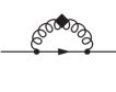
Figure 3.2: One-loop quark self energy with resummed gluon propagator.

The quark self energy will be used in the next chapter to compute the specific heat of normal cold dense quark matter. We will evaluate the quark self energy only on the light cone, since this is the quantity which enters the formula for the specific heat at leading order [see Eq. (4.15) below]. Furthermore it is sufficient for the computation of the specific heat to consider the fermionic quasiparticles in the vicinity of the Fermi surface. Thus the quark momentum is hard, while the momentum of the gluon in the one-loop self energy (see Fig. 3.2) may be arbitrarily soft. Therefore [75] we have to use a resummed gluon propagator in order to avoid an IR divergence in the quark self energy. For this reason we will review the computation of the HDL resummed gluon propagator in the next section.

3.2 Gluon self energy

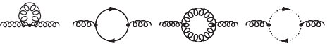
Figure 3.1: One-loop gluon self energy.

The gluon self energy at the one-loop level is given by the diagrams of Fig. 3.1. The second one of the four diagrams depends on the chemical potential and the temperature, while the three remaining ones give only finite temperature corrections to the gluon self energy. Below we will only need the gluon self energy at zero temperature, therefore we evaluate here only the diagram with a quark loop in Fig. 3.1. For QCD the diagram contains an additional factor of $\mathrm{Tr}[T^{a}T^{b}]={1\over 2}\delta^{ab}$ compared to the photon self energy in QED. In the following we shall drop the Kronecker delta, and define

$$g_{\rm eff}^{2}=\left\{\begin{array}[]{cc}\displaystyle\frac{g^{2}N_{f}}{2}\,,&{\rm QCD}\,,\\ &\\ g^{2}N_{f}\,,&{\rm QED}\,.\\ \end{array}\right.$$ (3.1)

Then our final results will be applicable both for QCD and QED.

In the imaginary time formalism [76] we get for the second diagram of Fig. 3.1

$$\Pi_{\mu\nu}(i\omega,q)=-g_{\rm eff}^{2}T\sum_{\omega_{n}}\int{d^{3}k\over(2\pi)^{3}}\mathrm{Tr}\left[\gamma_{\mu}S_{0}(K-Q)\gamma_{\nu}S_{0}(K)\right],$$ (3.2)

where $Q^{\mu}=(i\omega,{\bf q})$ and $K^{\mu}=(i\omega_{n},{\bf k})$, and the free quark propagator is given by

$$S_{0}(i\omega_{n},k)=\int_{-\infty}^{\infty}{dk_{0}\over 2\pi}{\not{K}\rho_{0}(K)\over k_{0}-i\omega_{n}-\mu}$$ (3.3)

with

$$\rho_{0}(K)=2\pi\mathrm{sgn}(k_{0})\,\delta\left(k_{0}^{2}-k^{2}\right)={\pi\over k}\left[\delta(k_{0}-k)-\delta(k_{0}+k)\right].$$ (3.4)

Using the methods outlined in appendix A it is straightforward to evaluate the Matsubara sum in Eq. (3.2),

$$T\sum_{\omega_{n}}{1\over k_{0}-i\omega_{n}-\mu}{1\over p_{0}-i\omega_{n}+i\omega-\mu}={n_{f}(k_{0}-\mu)-n_{f}(p_{0}-\mu)\over k_{0}-p_{0}-i\omega},$$ (3.5)

where $n_{f}$ is the Fermi-Dirac distribution defined in Eq. (A.13). After performing the Dirac trace in Eq. (3.2) we get [77],

$$\Pi_{\mu\nu}(i\omega,q)=-4g_{\rm eff}^{2}\int{d^{3}k\over(2\pi)^{3}}\int_{-\infty}^{\infty}{dk_{0}\over 2\pi}\int_{-\infty}^{\infty}{dp_{0}\over 2\pi}\rho_{0}(k_{0},k)\rho_{0}(p_{0},p)$$

$$\quad\times{n_{f}(k_{0}-\mu)-n_{f}(p_{0}-\mu)\over k_{0}-p_{0}-i\omega}\left(k_{\mu}p_{\nu}+p_{\mu}k_{\nu}-g_{\mu\nu}k\cdot p\right),$$ (3.6)

where ${\bf p}={\bf k}-{\bf q}$. Now we can perform the analytic continuation $i\omega\to q_{0}+i\eta$ to get the retarded self energy. Using

$${1\over x+i\eta}={\cal P}{1\over x}-\delta(x)$$ (3.7)

we can separate the real and imaginary parts of the self energy. It is convenient to define

$$\Pi_{G}:=g^{\mu\nu}\Pi_{\mu\nu},\quad\Pi_{H}:=u^{\mu}u^{\nu}\Pi_{\mu\nu},$$ (3.8)

with $u^{\mu}=(1,0,0,0)$. These two structure functions are related to the transverse and longitudinal self energies via

$$\Pi_{L}=-{q_{0}^{2}-q^{2}\over q^{2}}\Pi_{H},\quad\Pi_{T}={1\over 2}\left(-\Pi_{L}+\Pi_{G}\right).$$ (3.9)

After subtraction of the vacuum contribution one finds for the real parts [78]

$$\!\!\!\!\!\!\!\!\!\!\!\!\!\!\!\!\!\!\!\!\!\!\!\!\!\!\!\!\mathrm{Re}\Pi_{G}(q_{0},q)={g_{\rm eff}^{2}\over\pi^{2}}\int_{0}^{\infty}dk\,n(k)$$

$$\times\left(4k+{q_{0}^{2}-q^{2}\over 2q}\log\bigg{|}{(2k+q_{0}+q)(2k-q_{0}+q)\over(2k+q_{0}-q)(2k-q_{0}-q)}\bigg{|}\right),$$ (3.10)

$$\!\!\!\!\!\!\!\!\!\!\!\!\!\!\!\!\!\!\!\!\!\!\!\!\!\!\!\!\mathrm{Re}\Pi_{H}(q_{0},q)={g_{\rm eff}^{2}\over\pi^{2}}\int_{0}^{\infty}dk\,n(k)\bigg{[}2k\left(1-{q_{0}\over q}\log\bigg{|}{q_{0}+q\over q_{0}-q}\bigg{|}\right)$$

$$+{(2k+q_{0}+q)(2k+q_{0}-q)\over 4q}\log\bigg{|}{2k+q_{0}+q\over 2k+q_{0}-q}\bigg{|}$$

$$-{(2k-q_{0}-q)(2k-q_{0}+q)\over 4q}\log\bigg{|}{2k-q_{0}-q\over 2k-q_{0}+q}\bigg{|}\bigg{]},$$ (3.11)

where we use the abbreviation

$$n(k)={1\over 2}\left(n_{f}(k-\mu)+n_{f}(k+\mu)\right).$$ (3.12)

For the imaginary parts one finds [77]

$$\mathrm{Im}\Pi_{G,H}(q_{0},q)=-{1\over 2}(\pi^{+}_{G,H}(q_{0},q)-\pi^{+}_{G,H}(-p_{0},p)),$$ (3.13)

with

$$\!\!\!\!\!\pi^{+}_{G}(q_{0},q)={g_{\rm eff}^{2}\over\pi p}\int_{0}^{\infty}dk\,n(k)(q_{0}^{2}-q^{2})F(k,q_{0},q),$$ (3.14)

$$\!\!\!\!\!\pi^{+}_{H}(q_{0},q)={g_{\rm eff}^{2}\over 2\pi p}\int_{0}^{\infty}dk\,n(k)(2k+q-q_{0})(2k-q-q_{0})F(k,q_{0},q),\qquad$$ (3.15)

where

$$F(k,q_{0},q):=\mathrm{sgn}(k-q_{0})\Theta(|k-q|\leq|k-q_{0}|\leq|k+q|),$$ (3.16)

where we use the notation $\Theta({\rm true\ expression})=1$ and $\Theta({\rm false\ expression})=0$.

In general the remaining integrations over $k$ can be performed analytically only for the imaginary parts [77]. In the zero temperature limit, however, a closed result can be obtained also for the real parts. In this limit one finds for for $\Pi_{L}$ and $\Pi_{T}$ for $q_{0}\geq 0$ [77]

$$\!\!\!\!\!\!\!\!\!\!\!\!\!\!\!\!\!\!\!\!\!\!\!\mathrm{Re}\Pi_{L}(q_{0},q)\big{|}_{T=0}={g_{\rm eff}^{2}\left(q^{2}-q_{0}^{2}\right)\over 48\pi^{2}q^{2}}\Big{[}32\mu^{2}+{1\over q}N(q_{0},q)\Big{]},$$ (3.17)

$$\!\!\!\!\!\!\!\!\!\!\!\!\!\!\!\!\!\!\!\!\!\!\!\mathrm{Re}\Pi_{T}(q_{0},q)\big{|}_{T=0}={g_{\rm eff}^{2}\over 96\pi^{2}q^{3}}\Big{[}16\mu^{2}q\left(q^{2}+2q_{0}^{2}\right)$$

$$+\left(q^{2}-q_{0}^{2}\right)\left(6q^{2}M(q_{0},q)-N(q_{0},q)\right)\Big{]},$$ (3.18)

$$\!\!\!\!\!\!\!\!\!\!\!\!\!\!\!\!\!\!\!\!\!\!\!\mathrm{Im}\Pi_{L}(q_{0},q)\big{|}_{T=0}=-{g_{\rm eff}^{2}\left(q^{2}-q_{0}^{2}\right)\over 48\pi q^{3}}$$

$$\times\Big{[}W(q_{0},q)U(q_{0},q)-W(-q_{0},q)U(-q_{0},q)\Big{]},$$ (3.19)

$$\!\!\!\!\!\!\!\!\!\!\!\!\!\!\!\!\!\!\!\!\!\!\!\mathrm{Im}\Pi_{T}(q_{0},q)\big{|}_{T=0}={g_{\rm eff}^{2}\left(q^{2}-q_{0}^{2}\right)\over 96\pi q^{3}}$$

$$\!\!\!\!\!\times\Big{[}\left(W(q_{0},q)+6q^{2}\right)U(q_{0},q)-\left(W(-q_{0},q)+6q^{2}\right)U(-q_{0},q)\Big{]},$$ (3.20)

where we have used the abbreviations [77]

$$U(q_{0},q) = (2\mu-|q_{0}+q|)\Theta(2\mu-|q_{0}+q|),$$ (3.21)

$$V(q_{0},q) = (2\mu-q-q_{0})(2\mu+2q-q_{0}),$$ (3.22)

$$W(q_{0},q) = \Theta(q_{0}+q)V(q_{0},q)+\Theta(-q_{0}-q)V(-q_{0},-q),$$ (3.23)

$$R(q_{0},q) = (q_{0}+q)\log|q_{0}+q|-(2\mu+q_{0}+q)\log|2\mu+q_{0}+q|,$$ (3.24)

$$S(q_{0},q) = \left(-12\mu^{2}q_{0}+(2q-q_{0})(q+q_{0})^{2}\right)\log|q_{0}+q|$$ (3.25)

$$\quad+(2\mu-2q+q_{0})(2\mu+q+q_{0})^{2}\log|2\mu+q+q_{0}|,$$

$$M(q_{0},q) = R(q_{0},q)-R(q_{0},-q)+R(-q_{0},q)-R(-q_{0},-q),$$ (3.26)

$$N(q_{0},q) = S(q_{0},q)-S(q_{0},-q)+S(-q_{0},q)-S(-q_{0},-q).$$ (3.27)

If $q,q_{0}\ll\mu$ the leading contribution to the self energy is quadratic in $\mu$. This contribution comes from hard momenta in the quark loop ($k\sim\mu$), therefore the corresponding self energy ist called Hard Dense Loop (HDL) self energy [75, 79, 80, 81]. In the following we shall denote the HDL approximation with a tilde ($\tilde{\ }$). The explicit expressions are considerably simpler than the general ones given above [76],

$$\mathrm{Re}\tilde{\Pi}_{L}(q_{0},q) = 2m^{2}{q^{2}-q_{0}^{2}\over q^{2}}\left(1-{q_{0}\over 2q}\log\bigg{|}{q_{0}+q\over q_{0}-q}\bigg{|}\right),$$ (3.28)

$$\mathrm{Re}\tilde{\Pi}_{T}(q_{0},q) = m^{2}{q_{0}\over q}\left({q_{0}\over q}+{q^{2}-q_{0}^{2}\over 2q^{2}}\log\bigg{|}{q_{0}+q\over q_{0}-q}\bigg{|}\right),$$ (3.29)

$$\mathrm{Im}\tilde{\Pi}_{L}(q_{0},q) = m^{2}{q_{0}\left(q^{2}-q_{0}^{2}\right)\over q^{3}}\pi\Theta(q^{2}-q_{0}^{2}),$$ (3.30)

$$\mathrm{Im}\tilde{\Pi}_{T}(q_{0},q) = -m^{2}{q_{0}\left(q^{2}-q_{0}^{2}\right)\over 2q^{3}}\pi\Theta(q^{2}-q_{0}^{2}),$$ (3.31)

where $m^{2}=g_{\rm eff}^{2}\mu^{2}/(2\pi^{2})$. The leading finite temperature corrections have the same functional dependence on $q_{0}$ and $q$, one only has to include a finite temperature correction into $m^{2}$. For QCD one finds

$$m^{2}=N_{f}{g^{2}\mu^{2}\over 4\pi^{2}}+\left(N_{c}+{N_{f}\over 2}\right){g^{2}T^{2}\over 6},$$ (3.32)

where the contribution proportional to $N_{c}$ comes from the gluon and ghost loops in Fig. 3.1. The part of the gluon self energy which is quadratic in the temperature is called Hard Thermal Loop (HTL) self energy.

Using Dyson’s equation $\Pi_{\mu\nu}=D^{-1}_{\mu\nu}-D^{-1}_{0,\mu\nu}$ one can obtain the one-loop resummed gluon propagator. In the HDL approximation one finds in covariant gauge [76], using the tensors defined in Eqs. (2.43) and (2.44),

$$\tilde{D}_{\mu\nu}(q_{0},q)=-\tilde{D}_{T}\mathcal{A}_{\mu\nu}-\tilde{D}_{L}\mathcal{B}_{\mu\nu}-{\xi\over q^{2}-q_{0}^{2}}\mathcal{D}_{\mu\nu}$$ (3.33)

and in Coulomb gauge (see e.g. [82])

$$\tilde{D}_{\mu\nu}(q_{0},q)=-\tilde{D}_{T}\mathcal{A}_{\mu\nu}+\tilde{D}_{L}{q_{0}^{2}-q^{2}\over q^{2}}g_{\mu 0}g_{\nu 0}+\xi_{C}{Q_{\mu}Q_{\nu}\over q^{4}}$$ (3.34)

where

$$\tilde{D}_{L} = {1\over q^{2}-q_{0}^{2}+\tilde{\Pi}_{L}},$$ (3.35)

$$\tilde{D}_{T} = {1\over q^{2}-q_{0}^{2}+\tilde{\Pi}_{T}}.$$ (3.36)

The HDL spectral density for the transverse part is given by

$$\rho_{T}(q_{0},q)=2\,\mathrm{Im}\tilde{D}_{T}(q_{0}+i\eta,q).$$ (3.37)

In covariant gauge the longitudinal propagator contains an unphysical factor of $1/(q^{2}-q_{0}^{2})$ [60, 64], therefore one defines the longitudinal spectral density as

$$\rho_{L}(q_{0},q)=2{q_{0}^{2}-q^{2}\over q^{2}}\mathrm{Im}\tilde{D}_{L}(q_{0}+i\eta,q).$$ (3.38)

Both $\rho_{T}$ and $\rho_{L}$ contain a pole and a cut contribution. The explicit expressions can be found in [76], and are also given in appendix B for convenience. In terms of the spectral densities, the structure functions of the propagator can be written as [76]

$$\tilde{D}_{T}(q_{0},q) = \int_{-\infty}^{\infty}{dq_{0}^{\prime}\over 2\pi}{\rho_{T}(q_{0}^{\prime},q)\over q_{0}^{\prime}-q_{0}},$$ (3.39)

$${q_{0}^{2}-q^{2}\over q^{2}}\tilde{D}_{L}(q_{0},q) = \int_{-\infty}^{\infty}{dq_{0}^{\prime}\over 2\pi}{\rho_{L}(q_{0}^{\prime},q)\over q_{0}^{\prime}-q_{0}}-{1\over q^{2}}.$$ (3.40)

3.3 Fermion self energy on the light cone

The fermion self energy is defined through

$$S^{-1}(P)=S_{0}^{-1}(P)+\Sigma(P),$$ (3.41)

where $S_{0}(P)=-(P\!\!\!\!/)^{-1}$ is the free fermion propagator, and $P^{\mu}=(p^{0},{\bf p})$ with $p^{0}=i\omega_{n}+\mu$, $\omega_{n}=(2n+1)\pi T$ in the imaginary time formalism, and $P^{\mu}=(E,{\bf p})$ after analytic continuation to Minkowski space.

With the energy projection operators

$$\Lambda_{\bf p}^{\pm}={1\over 2}(1\pm\gamma_{0}\gamma^{i}\hat{p}^{i})$$ (3.42)

we decompose $\Sigma(P)$ in the quasiparticle and antiquasiparticle self energy,

$$\Sigma(P)=\gamma_{0}\Lambda_{\bf p}^{+}\Sigma_{+}(P)-\gamma_{0}\Lambda_{\bf p}^{-}\Sigma_{-}(P),$$ (3.43)

and

$$\gamma_{0}S^{-1}=S_{+}^{-1}\Lambda_{\bf p}^{+}+S_{-}^{-1}\Lambda_{\bf p}^{-}$$ (3.44)

so that $S_{\pm}^{-1}=-[p^{0}\mp(|\mathbf{p}|+\Sigma_{\pm})]$.

The one-loop fermion self energy is given by

$$\Sigma(P)=-g^{2}C_{f}T\sum_{\omega}\int{d^{3}q\over(2\pi)^{3}}\,\gamma^{\mu}S_{0}(P-Q)\gamma^{\nu}D_{\mu\nu}(Q),$$ (3.45)

where $D_{\mu\nu}$ is the gauge boson propagator.

Following [83] we introduce an intermediate scale $q^{*}$, such that $m\ll q^{*}\ll\mu$, and we divide the $q$-integration into a soft part ($q<q^{*}$) and a hard part ($q>q^{*}$),

$$\Sigma_{+}=\Sigma_{+}^{\mathrm{(s)}}+\Sigma_{+}^{\mathrm{(h)}}.$$ (3.46)

For the hard part we can use the free gluon propagator, whereas for the soft part we shall use the HDL resummed gluon propagator.

The hard part of the fermion self energy on the light cone in a general Coulomb gauge is given by the gauge independent expression

$$\!\!\!\!\!\!\!\Sigma_{+}^{\mathrm{(h)}}(E)=-{g^{2}C_{f}\over 8\pi^{2}}\int_{q^{*}}^{\infty}dq\,q^{2}\int_{-1}^{1}dt\int_{-\infty}^{\infty}dr_{0}\left[\delta(r_{0}-r)-\delta(r_{0}+r)\right]$$

$$\times\Bigg{\{}2\left(\mathrm{sgn}(r_{0})-\hat{\bf p}\!\cdot\!\hat{\bf q}\>\hat{\bf r}\!\cdot\!\hat{\bf q}\right)\int_{-\infty}^{\infty}dq_{0}{1\over 2q}\left[\delta(q_{0}-q)-\delta(q_{0}+q)\right]$$

$$\quad\times{1+n_{b}(q_{0})-n_{f}(r_{0}-\mu)-\Theta(q_{0})+\Theta(-r_{0})\over r_{0}+q_{0}-E-i\eta}$$

$$\quad+\left(\mathrm{sgn}(r_{0})+\hat{\bf r}\!\cdot\!\hat{\bf p}\right){1\over q^{2}}\left[n_{f}(r_{0}-\mu)-\Theta(-r_{0})\right]\Bigg{\}},$$ (3.47)

where ${\bf r}={\bf p}-{\bf q}$ and $E=p$. The distribution functions $n_{b}$ and $n_{f}$ are given by Eqs. (A.5) and (A.13). In Eq. (3.47) we have subtracted the vacuum parts of the distribution functions, since we know anyway that the vacuum part of the fermion self energy on the light cone vanishes because of gauge and Lorentz invariance. This subtraction is in fact necessary, because otherwise we would get a spurious vacuum contribution coming from the fact the we do not use an $O(4)$ invariant cutoff for the energy-momentum integration. The finite-$T$ and finite-$\mu$ parts, however, are not affected by these subtleties in the UV region.

After performing the angular integration we find

$$\Sigma_{+}^{\mathrm{(h)}}(E)={g^{2}C_{f}\over 8\pi^{2}p^{2}}\int_{q^{*}}^{\infty}dq\,q\,\bigg{\{}2\left(q-|p-q|+p\coth\left({q\over 2T}\right)\right)$$

$$\quad\qquad\qquad+T\log\left[{\left(1+e^{(|p-q|-\mu)/T}\right)\left(1+e^{(|p-q|+\mu)/T}\right)\over\left(1+e^{(p+q-\mu)/T}\right)\left(1+e^{(p+q+\mu)/T}\right)}\right]\bigg{\}}.$$ (3.48)

The integral is finite in the limit $q^{*}\to 0$, with the result

$$\Sigma_{+}^{\mathrm{(h)}}={M_{\infty}^{2}\over 2p}(1+\mathcal{O}(T^{2}/\mu^{2})),$$ (3.49)

with $M_{\infty}^{2}=g^{2}C_{f}\mu^{2}/(4\pi^{2})$. Here $q^{*}$ enters as a correction proportional to $(q^{*}/\mu)^{2}$, so that we can send $q^{*}$ to zero. Conversely we expect that in the soft contribution we should be able to send $q^{*}$ to infinity without encountering divergences, as will indeed be the case, but only after all soft contributions are added together.

For the soft part one finds on the light cone in a general Coulomb gauge the gauge independent expression [82]

$$\!\!\!\!\!\!\!\!\!\!\!\!\!\!\!\!\Sigma_{\pm}^{\mathrm{(s)}}(E)=-{g^{2}C_{f}\over 8\pi^{2}}\int_{0}^{q^{*}}dq\,q^{2}\int_{-1}^{1}dt\int_{-\infty}^{\infty}dr_{0}\left[\delta(r_{0}-r)-\delta(r_{0}+r)\right]$$

$$\times\Bigg{\{}2\left(\pm\mathrm{sgn}(r_{0})-\hat{\bf p}\!\cdot\!\hat{\bf q}\>\hat{\bf r}\!\cdot\!\hat{\bf q}\right)\int_{-\infty}^{\infty}{dq_{0}\over 2\pi}\rho_{T}(q_{0},q){1+n_{b}(q_{0})-n_{f}(r_{0}-\mu)\over r_{0}+q_{0}\mp|E|-i\eta}$$

$$\quad+\left(\pm\mathrm{sgn}(r_{0})+\hat{\bf r}\!\cdot\!\hat{\bf p}\right)\bigg{[}\int_{-\infty}^{\infty}{dq_{0}\over 2\pi}\rho_{L}(q_{0},q){1+n_{b}(q_{0})-n_{f}(r_{0}-\mu)\over r_{0}+q_{0}\mp|E|-i\eta}$$

$$\quad-{1\over q^{2}}\left({1\over 2}-n_{f}(r_{0}-\mu)\right)\bigg{]}\Bigg{\}},$$ (3.50)

where $E=\pm p$, and $\rho_{T}$ and $\rho_{L}$ are the spectral densities of transverse and longitudinal gauge bosons, as given in Eqs. (3.37) and (3.38). We may use $q\ll|E|,r$ because of $q<q^{*}$ and $|E|\sim\mu$. Depending on the sign of $E$, we can drop the term $\delta(r_{0}+r)$ or the term $\delta(r_{0}-r)$ in Eq. (3.50), since its contribution is suppressed with $\sim q/E$ compared to the remaining contribution. Then we find for the soft contribution to the real part of $\Sigma_{+}$

$$\!\!\!\!\!\!\!\!\!\!\mathrm{Re}\Sigma_{+}^{\mathrm{(s)}}=-{g^{2}C_{f}\over 8\pi^{2}}\int_{0}^{q^{*}}dq\,q^{2}\int_{-1}^{1}dt\bigg{[}\int_{-\infty}^{\infty}{dq_{0}\over\pi}\left[(1-t^{2})\rho_{T}(q_{0},q)+\rho_{L}(q_{0},q)\right]$$

$$\times\>\mathcal{P}{1+n_{b}(q_{0})-n_{f}(E-\mu-qt)\over q_{0}-qt}-{1\over q^{2}}\left(1-2n_{f}(E-\mu-qt)\right)\bigg{]}.$$ (3.51)

This quantity vanishes for $E=\mu$ by symmetric integration. After performing the $q_{0}$-integration we therefore have

$$\mathrm{Re}\Sigma_{+}^{\mathrm{(s)}}={g^{2}C_{f}\over 4\pi^{2}}\int_{0}^{q^{*}}dq\,q^{2}\int_{-1}^{1}dt\left(n_{f}(E-\mu-qt)-n_{f}(-qt)\right)$$

$$\qquad\qquad\qquad\times(1-t^{2})\left[\mathrm{Re}\tilde{D}_{T}(qt,q)-\mathrm{Re}\tilde{D}_{L}(qt,q)\right],$$ (3.52)

where $\tilde{D}_{T}$ and $\tilde{D}_{L}$ are given in Eqs. (3.35) and (3.36), respectively. For $\mathrm{Im}\Sigma_{+}$ (which receives no hard contribution) we find in an analogous way

$$\!\!\!\!\!\!\!\!\!\!\mathrm{Im}\Sigma_{+}=-{g^{2}C_{f}\over 8\pi^{2}}\int_{0}^{q^{*}}dq\,q^{2}\int_{-1}^{1}dt\left((1-t^{2})\rho_{T}(qt,q)+\rho_{L}(qt,q)\right)$$

$$\qquad\times\>\left[1+n_{b}(qt)-n_{f}(E-\mu-qt)\right].$$ (3.53)

The antiquasiparticle self energy $\Sigma_{-}^{\mathrm{(s)}}$ is obtained by inserting negative values of $E$ in the above expressions for $\Sigma_{+}^{\mathrm{(s)}}$ and including an overall factor $(-1)$. With $\mu>0$ we can then replace $n_{f}(E-\mu-qt)$ by 1.

3.4 Expansion for small $|E-\mu|$ and small $T$

In this section we will perform an expansion of $\Sigma_{+}$ in the region

$$T\sim|E-\mu|\ll g\mu\ll\mu.$$ (3.54)

This region is relevant for the computation of the low temperature specific heat, see chapter 4. We will use the expansion parameter $a:=T/m$, and we define $\lambda:=(E-\mu)/T$. From (3.54) we have $a\ll 1$ and $\lambda\sim\mathcal{O}(1)$.

3.4.1 The first few terms in the series

In the part with the transverse gluon propagator we substitute

$$q=ma^{1/3}z,\quad t=a^{2/3}v/z.$$ (3.55)

After expanding the integrand with respect to $a$ we find for the transverse contribution

$$\!\!\!\!\!\!\!\!\!\!\mathrm{Re}\Sigma^{\mathrm{(s)}}_{+(T)}=-{g^{2}C_{f}ma\over\pi^{2}}\int_{-{q^{*}\over am}}^{q^{*}\over am}dv\int_{a^{2/3}|v|}^{q^{*}\over a^{1/3}m}dz\,{e^{\lambda}-1\over(1+e^{v})(1+e^{\lambda-v})}$$

$$\!\!\!\!\times\bigg{[}{z^{5}\over v^{2}\pi^{2}+4z^{6}}+{2v^{2}z(v^{2}\pi^{2}-4z^{6})\over(v^{2}\pi^{2}+4z^{6})^{2}}a^{2/3}-{16v^{4}z^{3}(3v^{2}\pi^{2}-4z^{6})\over(v^{2}\pi^{2}+4z^{6})^{3}}a^{4/3}+\ldots\bigg{]}.$$

(3.56)

The $z$-integrations are straightforward. In the $v$-integrals we may send the integration limits to $\pm\infty$. Using the formulae

$$\int_{-\infty}^{\infty}dv{e^{\lambda}-1\over(1+e^{v})(1+e^{\lambda-v})}|v|^{\alpha}$$

$$\qquad=\Gamma(\alpha+1)\left[\mathrm{Li}_{\alpha+1}(-e^{-\lambda})-\mathrm{Li}_{\alpha+1}(-e^{\lambda})\right]\quad\forall\alpha\geq 0,\quad$$ (3.57)

$$\int_{-\infty}^{\infty}dv{e^{\lambda}-1\over(1+e^{v})(1+e^{\lambda-v})}\log|v|$$

$$\qquad=-\gamma_{E}\lambda+{\partial\over\partial\alpha}\left(\mathrm{Li}_{\alpha+1}(-e^{-\lambda})-\mathrm{Li}_{\alpha+1}(-e^{\lambda})\right)\Big{|}_{\alpha=0},$$ (3.58)

we find, neglecting terms which are suppressed at least with $(m/q^{*})^{4}$,

$$\!\!\!\!\!\!\!\!\!\!\!\!\mathrm{Re}\Sigma^{\mathrm{(s)}}_{+(T)}=-g^{2}C_{f}m$$

$$\!\!\!\!\!\times\Bigg{\{}{a\over 12\pi^{2}}\left[\lambda\log\left({2(q^{*})^{3}\over am^{3}\pi}\right)+\gamma_{E}\lambda-{\partial\over\partial\alpha}\left(\mathrm{Li}_{\alpha+1}(-e^{-\lambda})-\mathrm{Li}_{\alpha+1}(-e^{\lambda})\right)\Big{|}_{\alpha=0}\right]$$

$$+{2^{1/3}a^{5/3}\over 9\sqrt{3}\pi^{7/3}}\Gamma\left(\textstyle{5\over 3}\right)\left(\mathrm{Li}_{5/3}(-e^{-\lambda})-\mathrm{Li}_{5/3}(-e^{\lambda})\right)$$

$$-20{2^{2/3}a^{7/3}\over 27\sqrt{3}\pi^{11/3}}\Gamma\left(\textstyle{7\over 3}\right)\left(\mathrm{Li}_{7/3}(-e^{-\lambda})-\mathrm{Li}_{7/3}(-e^{\lambda})\right)$$

$$+{8(24-\pi^{2})a^{3}\log a\over 27\pi^{6}}\lambda(\lambda^{2}+\pi^{2})+\mathcal{O}(a^{3})\Bigg{\}}.$$ (3.59)

In the longitudinal part we substitute $q=mx$ and $t=au/x$. In a similar way as for the transverse part we find

$$\mathrm{Re}\Sigma^{\mathrm{(s)}}_{+(L)}=-g^{2}C_{f}m\left[{a\lambda\over 8\pi^{2}}\log\left({2m^{2}\over(q^{*})^{2}}\right)-{(\pi^{2}-4)a^{3}\log a\over 96\pi^{2}}\lambda(\lambda^{2}+\pi^{2})+\mathcal{O}(a^{3})\right].$$ (3.60)

Turning now to $\mathrm{Im}\Sigma_{+}$ we notice that it vanishes at $E=\mu$ only in the case of $T=0$. For finite temperature, however small, there is an IR divergent contribution in the transverse sector [76],

$$\mathrm{Im}\Sigma_{+(T)}\big{|}_{E=\mu}=-{g^{2}C_{f}T\over 4\pi}\log{m\over\Lambda_{\rm IR}}$$ (3.61)

where the infrared cutoff may be provided at finite temperature by the nonperturbative magnetic screening mass of QCD. In QED, where no magnetostatic screening is possible, a resummation of these singularities leads to nonexponential damping behavior [84].

After subtraction of the energy independent part we have

$$\mathrm{Im}\Sigma_{+}-\mathrm{Im}\Sigma_{+}\big{|}_{E=\mu}={g^{2}C_{f}\over 8\pi^{2}}\int_{0}^{q^{*}}dq\,q^{2}\int_{-1}^{1}dt\left(n_{f}(E-\mu-qt)-n_{f}(-qt)\right)$$

$$\qquad\qquad\qquad\qquad\qquad\qquad\times\left[(1-t^{2})\rho_{T}(qt,q)+\rho_{L}(qt,q)\right].$$ (3.62)

Following the steps which led to Eq. (3.56), we find for the transverse contribution

$$\!\!\!\!\!\!\!\!\!\!\!\mathrm{Im}\Sigma_{+(T)}-\mathrm{Im}\Sigma_{+(T)}\big{|}_{E=\mu}={g^{2}C_{f}ma\over 2\pi}\int_{-{q^{*}\over am}}^{q^{*}\over am}dv\int_{a^{2/3}|v|}^{q^{*}\over a^{1/3}m}dz\,{e^{\lambda}-1\over(1+e^{v})(1+e^{\lambda-v})}$$

$$\qquad\times\bigg{[}-{z^{2}v\over v^{2}\pi^{2}+4z^{6}}+{16v^{3}z^{4}\over(v^{2}\pi^{2}+4z^{6})^{2}}a^{2/3}+{16v^{5}(v^{2}\pi^{2}-12z^{6})\over(v^{2}\pi^{2}+4z^{6})^{3}}a^{4/3}+\ldots\bigg{]}.$$

Using the formula

$$\!\!\!\!\!\!\!\!\!\int_{-\infty}^{\infty}dv{e^{\lambda}-1\over(1+e^{v})(1+e^{\lambda-v})}|v|^{\alpha}\mathrm{sgn}(\alpha)$$

$$\!\!\!\!=-\Gamma(\alpha+1)\left[\mathrm{Li}_{\alpha+1}(-e^{-\lambda})+\mathrm{Li}_{\alpha+1}(-e^{\lambda})+2\left(1-2^{-\alpha}\right)\zeta(\alpha+1)\right]\quad\forall\alpha\geq 0$$

we find in a similar way as above

$$\!\!\!\!\!\!\!\!\!\!\!\!\!\!\!\!\mathrm{Im}\Sigma_{+(T)}-\mathrm{Im}\Sigma_{+(T)}^{\mathrm{(s)}}\big{|}_{E=\mu}={g^{2}C_{f}m}\Bigg{\{}-{a\over 12\pi}\log\cosh\left({\lambda\over 2}\right)$$

$$-{2^{1/3}a^{5/3}\over 9\pi^{7/3}}\Gamma\left(\textstyle{5\over 3}\right)\left(\mathrm{Li}_{5/3}(-e^{-\lambda})+\mathrm{Li}_{5/3}(-e^{\lambda})+2\left(1-2^{-2/3}\right)\zeta\left(\textstyle{5\over 3}\right)\right)$$

$$-20{2^{2/3}a^{7/3}\over 27\pi^{11/3}}\Gamma\left(\textstyle{7\over 3}\right)\left(\mathrm{Li}_{7/3}(-e^{-\lambda})+\mathrm{Li}_{7/3}(-e^{\lambda})+2\left(1-2^{-4/3}\right)\zeta\left(\textstyle{7\over 3}\right)\right)$$

$$+\mathcal{O}(a^{3})\Bigg{\}}.$$ (3.65)

For the longitudinal part we obtain

$$\mathrm{Im}\Sigma_{+(L)}-\mathrm{Im}\Sigma_{+(L)}^{\mathrm{(s)}}\big{|}_{E=\mu}=-{g^{2}C_{f}m}\left[{a^{2}\lambda^{2}\over 64\sqrt{2}}+\mathcal{O}(a^{3})\right].$$ (3.66)

Putting the pieces together, and using the abbreviation $\varepsilon=E-\mu$, we obtain for the real part

$$\!\!\!\!\!\!\!\!\!\!\!\!\mathrm{Re}\Sigma_{+}={M_{\infty}^{2}\over 2E}-g^{2}C_{f}m\,\mathrm{sgn}(\varepsilon)\Bigg{\{}{|\varepsilon|\over 12\pi^{2}m}\left[\log\left({4\sqrt{2}m\over\pi Tf_{1}(\varepsilon/T)}\right)+1\right]$$

$$+{2^{1/3}\sqrt{3}\over 45\pi^{7/3}}\left({T\over m}f_{2}\left({\varepsilon\over T}\right)\right)^{5/3}-20{2^{2/3}\sqrt{3}\over 189\pi^{11/3}}\left({T\over m}f_{3}\left({\varepsilon\over T}\right)\right)^{7/3}$$

$$-{6144-256\pi^{2}+36\pi^{4}-9\pi^{6}\over 864\pi^{6}}\left({T\over m}f_{4}\left({\varepsilon\over T}\right)\right)^{3}\log\left({m\over T}\right)+\left({T\over m}\right)^{3}c_{3}\left({\varepsilon\over T}\right)$$

$$+\mathcal{O}\left({T\over m}\right)^{11/3}\Bigg{\}},$$ (3.67)

where

$$f_{1}(\lambda) = \exp\left[1-\gamma_{E}+{1\over\lambda}{\partial\over\partial\alpha}\left(\mathrm{Li}_{\alpha+1}(-e^{-\lambda})-\mathrm{Li}_{\alpha+1}(-e^{\lambda})\right)\Big{|}_{\alpha=0}\right],$$ (3.68)

$$f_{2}(\lambda) = \left|\Gamma\left(\textstyle{8\over 3}\right)\left(\mathrm{Li}_{5/3}(-e^{-\lambda})-\mathrm{Li}_{5/3}(-e^{\lambda})\right)\right|^{3/5},$$ (3.69)

$$f_{3}(\lambda) = \left|\Gamma\left(\textstyle{10\over 3}\right)\left(\mathrm{Li}_{7/3}(-e^{-\lambda})-\mathrm{Li}_{7/3}(-e^{\lambda})\right)\right|^{3/7},$$ (3.70)

$$f_{4}(\lambda) = \left|\lambda(\lambda^{2}+\pi^{2})\right|^{1/3}.$$ (3.71)

The determination of the function $c_{3}(\lambda)$ requires resummation of IR enhanced contributions, which will be discussed in the next subsection. We note furthermore that the dependence on $q^{*}$ indeed drops out in the sum of the transverse and longitudinal parts.

The functions $f_{i}(\lambda)$ show a simple asymptotic behavior. In the zero temperature limit ($|\lambda|\to\infty$) we have $f_{i}(\lambda)\to|\lambda|$. If the temperature is much higher than $|E-\mu|$ (i.e. $\lambda\to 0$) we have $f_{1}(\lambda)\to c_{0}:={\pi\over 2}\exp(1-\gamma_{E})=2.397357\ldots$ and $f_{2,3,4}(\lambda)\to 0$. For $|\lambda|\gg c_{0}$ or $|\lambda|\ll c_{0}$ we may approximate $f_{1}(\lambda)$ with $\mathrm{max}(c_{0},|\lambda|)$, which is qualitatively the result quoted in [86]. It should be noted, however, that the calculation of Ref. [86] only took into account transverse gauge bosons, and therefore the scale under the logarithm and its parametric dependence on the coupling was not correctly rendered.

For the imaginary part we find

$$\mathrm{Im}\Sigma_{+}-\mathrm{Im}\Sigma_{+}\big{|}_{E=\mu}=g^{2}C_{f}m\bigg{[}-{T\over 24\pi m}g_{1}\left({\varepsilon\over T}\right)+3{2^{1/3}\over 45\pi^{7/3}}\left({T\over m}g_{2}\left({\varepsilon\over T}\right)\right)^{5/3}$$

$$\quad\qquad\qquad-{1\over 64\sqrt{2}}\left({T\over m}g_{3}\left({\varepsilon\over T}\right)\right)^{2}+20{2^{2/3}\over 63\pi^{11/3}}\left({T\over m}g_{4}\left({\varepsilon\over T}\right)\right)^{7/3}$$

$$\qquad\qquad\qquad+\left({T\over m}\right)^{3}d_{3}\left({\varepsilon\over T}\right)\bigg{)}+\mathcal{O}\left({T\over m}\right)^{11/3}\bigg{]},$$ (3.72)

where

$$\!\!\!\!\!\!\!\!\!\!\!\!\!\!g_{1}(\lambda) \!\!=\!\! 2\log\cosh\left({\lambda\over 2}\right),$$ (3.73)

$$\!\!\!\!\!\!\!\!\!\!\!\!\!\!g_{2}(\lambda) \!\!=\!\! \left[-\Gamma\left(\textstyle{8\over 3}\right)\left(\mathrm{Li}_{5/3}(-e^{-\lambda})+\mathrm{Li}_{5/3}(-e^{\lambda})+2\left(1-2^{-2/3}\right)\zeta\left(\textstyle{5\over 3}\right)\right)\right]^{3/5},$$ (3.74)

$$\!\!\!\!\!\!\!\!\!\!\!\!\!\!g_{3}(\lambda) \!\!=\!\! |\lambda|,$$ (3.75)

$$\!\!\!\!\!\!\!\!\!\!\!\!\!\!g_{4}(\lambda) \!\!=\!\! \left[-\Gamma\left(\textstyle{10\over 3}\right)\left(\mathrm{Li}_{7/3}(-e^{-\lambda})+\mathrm{Li}_{7/3}(-e^{\lambda})+2\left(1-2^{-4/3}\right)\zeta\left(\textstyle{7\over 3}\right)\right)\right]^{3/7}.$$ (3.76)

In the zero temperature limit we have $g_{i}(\lambda)\to|\lambda|$. If the temperature is much higher than $|E-\mu|$ we have $g_{i}(\lambda)\to 0$. Again the determination of the function $d_{3}(\lambda)$ requires resummation of IR enhanced contributions, which will be discussed in the next subsection.

Explicitly, our $T=0$ result reads

$$\Sigma_{+}\big{|}_{T=0} = {M_{\infty}^{2}\over 2E}-g^{2}C_{f}m\,\Bigg{\{}{\varepsilon\over 12\pi^{2}m}\left[\log\left({4\sqrt{2}m\over\pi|\varepsilon|}\right)+1\right]+{i|\varepsilon|\over 24\pi m}$$ (3.77)

$$\!\!\!\!\!\!\!+{2^{1/3}\sqrt{3}\over 45\pi^{7/3}}\left({|\varepsilon|\over m}\right)^{5/3}(\mathrm{sgn}(\varepsilon)-\sqrt{3}i)$$

$$\!\!\!\!\!\!\!+{i\over 64\sqrt{2}}\left({\varepsilon\over m}\right)^{2}-20{2^{2/3}\sqrt{3}\over 189\pi^{11/3}}\left({|\varepsilon|\over m}\right)^{7/3}(\mathrm{sgn}(\varepsilon)+\sqrt{3}i)$$

$$\!\!\!\!\!\!\!-{6144-256\pi^{2}+36\pi^{4}-9\pi^{6}\over 864\pi^{6}}\left({\varepsilon\over m}\right)^{3}\left[\log\left({m\,0.927\ldots\over|\varepsilon|}\right)-{i\pi\mathrm{sgn}(\varepsilon)\over 2}\right]$$

$$\!\!\!\!\!\!\!+\mathcal{O}\bigg{(}\left({|\varepsilon|\over m}\right)^{11/3}\bigg{)}\Bigg{\}},$$

where we have included the zero temperature limits of $c_{3}$ and $d_{3}$, which will be derived in the next subsection. We observe that the self energy at $T=0$ is at leading order proportional to $\varepsilon\log|\varepsilon|$, which is nonanalytic at $\varepsilon=0$. This behavior is a consequence of quasistatic chromomagnetic fields, which are only dynamically screened. On the other hand chromoelectric fields, which are screened by the Debye mass, give an analytic term ($\propto\varepsilon$) in the self energy at leading order, and nonanalytic contributions ($\propto\varepsilon^{3}\log|\varepsilon|$) only at higher orders.

Apart from the first logarithmic term, the leading imaginary parts contributed by the transverse and longitudinal gauge bosons were known previously [82, 87, 88]. As our results show, the damping rate obtained by adding these two leading terms [82, 87] is actually incomplete beyond the leading term, because the subleading transverse term of order $|\varepsilon|^{5/3}$ is larger than the leading contribution from $\Sigma_{L}$.

3.4.2 Evaluation of the $a^{3}$-coefficient

We write the function $c_{3}(\lambda)$ in Eq. (3.67) as the sum of the transverse and the longitudinal contribution, $c_{3}=c_{3T}+c_{3L}$. The terms through order $a^{3}$ in the integrand of Eq. (3.56) give the following contribution to $c_{3T}(\lambda)$,

$$\!\!\!\!\!\!\!\!\!\!\!\!\!\!\!\!c_{3T}^{(1)}(\lambda)={1\over 3}\lambda(\lambda^{2}+\pi^{2})$$

$$\times\left[{1\over\pi^{4}}+{2\over\pi^{6}}\left(-8\left(11-6\log\left({\textstyle{\pi\over 2}}\right)\right)+2\pi^{2}\left(1-\log\left({\textstyle{\pi\over 2}}\right)\right)\right)\right]$$

$$\!\!\!\!-{8(24-\pi^{2})\over 9\pi^{6}}\bigg{[}{1\over 6}(3-2\gamma_{E})\lambda(\lambda^{2}+\pi^{2})$$

$$\quad+2{\partial\over\partial\alpha}\left(\mathrm{Li}_{\alpha+3}(-e^{-\lambda})-\mathrm{Li}_{\alpha+3}(-e^{\lambda})\right)\Big{|}_{\alpha=0}\bigg{]},$$ (3.78)

Evaluating explicitly the next few terms in the expansion of the integrand, one finds additional contributions of order $a^{3}$. They arise from the fact that the $z$-integrations would be IR divergent, being screened only by $z_{min}=a^{2/3}|v|$. Therefore also terms which are formally of higher order in the integrand contribute to the order $a^{3}$ in the self energy. In the following we will perform a systematic summation of all these terms.

With the substitution (3.55) the transverse gluon self energy in the HDL approximation can be written as

$$\tilde{\Pi}_{T}(qt,q)=g_{\rm eff}^{2}\mu^{2}H_{T}\left({a^{2/3}v\over z}\right),$$ (3.79)

with some function $H_{T}$. We may neglect the term $q^{2}-q_{0}^{2}$ from the free propagator, because this term does not become singular for small $x$. After expansion of the integrand with respect to $a$ as in Eq. (3.56) we get then integrals of the following type contributing to the self energy,

$$ma^{5/3}\int_{z_{min}}dz\,z\left({a^{2/3}v\over z}\right)^{n}\sim{ma^{3}v^{n}|v|^{2-n}\over{n-2}}={ma^{3}v^{2}\over{n-2}}.$$ (3.80)

[In the last step we have used the fact that $\mathrm{Re}\tilde{D}_{T}(qt,q)$ is an even function of $t$.] Now we see clearly that from arbitrary powers of $a$ in the integrand we get contributions to the order $a^{3}$ in $\mathrm{Re}\Sigma_{+}$. The case $n=2$ corresponds to the term of order $a^{3}\log a$, which we have evaluated already in the previous section. As we are interested only in contributions from the IR region, we may take $\infty$ as upper integration limit in Eq. (3.80), since for $n>2$ we get then no contribution from the upper integration limit. [The cases $n<2$ have been evaluated explicitly in Eq. (3.78).] Furthermore we see from Eq. (3.80) that from the $v$-integration we always get a factor

$$\int_{-\infty}^{\infty}dv\,{e^{\lambda}-1\over(1+e^{v})(1+e^{\lambda-v})}v^{2}={1\over 3}\lambda(\lambda^{2}+\pi^{2}).$$ (3.81)

Now we can write the function $c_{3T}(\lambda)$ as

$$c_{3T}(\lambda)=c_{3T}^{(1)}(\lambda)-{\lambda(\lambda^{2}+\pi^{2})m^{2}\over 12\pi^{2}\tilde{b}^{9}}\int_{\tilde{b}^{2}}^{\infty}dz\,z$$

$$\qquad\times\sum_{n=11}^{\infty}{\tilde{b}^{n}\over n!}\left(\left[{\partial^{n}\over\partial\tilde{b}^{n}}\tilde{b}^{5}\left(1-{\tilde{b}^{2}\over z}\right)\mathrm{Re}\tilde{D}_{T}^{\prime}(m\tilde{b}^{3},m\tilde{b}z)\right]\Bigg{|}_{\tilde{b}=0}\right),$$ (3.82)

where $\tilde{b}=a^{3}$, and the prime denotes the omission of the tree level propagator. Eq. (3.82) is in fact independent of $\tilde{b}$, therefore we may simply set $\tilde{b}=1$. Summing up the (Taylor) series we find

$$c_{3T}(\lambda)=c_{3T}^{(1)}+{\lambda(\lambda^{2}+\pi^{2})\over 3}J_{1}$$ (3.83)

with

$$J_{1}=-{1\over 4\pi^{2}}\int_{1}^{\infty}dz\left[-{8z\over\pi^{2}}+{16(24-\pi^{2})\over 3\pi^{4}z}+{z^{2}-1\over z}m^{2}\mathrm{Re}{\tilde{D}_{T}^{\prime}}|_{q\to zq_{0}}\right].$$ (3.84)

This integral can probably not be done analytically. Numerically one finds readily $J_{1}=0.000233964448\ldots$.

For the longitudinal part a completely analogous calculation gives

$$\!\!\!\!\!\!\!\!\!\!\!\ c_{3L}={1\over 3}\lambda(\lambda^{2}+\pi^{2})\left[-{1\over 16\pi^{2}}-{1\over 128\pi^{2}}\left(8-3\pi^{2}+2(\pi^{2}-4)\log 2\right)+J_{2}\right]$$

$$+{4(\pi^{2}-4)\over 128\pi^{2}}\bigg{[}{1\over 6}(3-2\gamma_{E})\lambda(\lambda^{2}+\pi^{2})$$

$$\quad+2{\partial\over\partial\alpha}\left(\mathrm{Li}_{\alpha+3}(-e^{-\lambda})-\mathrm{Li}_{\alpha+3}(-e^{\lambda})\right)\Big{|}_{\alpha=0}\bigg{]},$$ (3.85)

with

$$J_{2}=-{1\over 4\pi^{2}}\int_{1}^{\infty}dz\left[{z\over 2}-{\pi^{2}-4\over 8z}+zm^{2}\mathrm{Re}\tilde{D}_{L}^{\prime}|_{q\to zq_{0}}\right].$$ (3.86)

Numerically one has $J_{2}=0.000250187944\ldots$

The constant under the logarithm in the fourth line of Eq. (3.77) can be determined from the zero temperature limit of $c_{3}(\lambda)$, with the result

$$\exp\Bigg{\{}{1\over 12(6144-256\pi^{2}+36\pi^{4}-9\pi^{6})}\bigg{[}-9\pi^{6}(-5+6\log 2)$$

$$+72\pi^{4}(-4+3\log 2)+128\pi^{2}(31-12\log({\textstyle{\pi\over 2}}))-6144(7-6\log({\textstyle{\pi\over 2}}))$$

$$+3456\pi^{6}(J_{1}+J_{2})\bigg{]}\Bigg{\}}=0.92789731088\ldots$$ (3.87)

Let us turn now to the imaginary part. The function $d_{3}(\lambda)$ in Eq. (3.72) can be determined by summing up IR enhanced contributions in a similar way as in the computation of $c_{3}(\lambda)$. We find

$$d_{3}(\lambda)=\left({1920-56\pi^{2}-9\pi^{4}\over 144\pi^{5}}+J_{3}+J_{4}\right)\left[-2(\mathrm{Li}_{3}(-e^{-\lambda})+\mathrm{Li}_{3}(-e^{\lambda}))-3\zeta(3)\right],$$ (3.88)

with

$$J_{3} = {1\over 8\pi^{2}}\int_{1}^{\infty}\left[-{4z^{2}\over\pi}+{64\over\pi^{3}}+{z^{2}-1\over z}m^{2}\bar{\rho}_{T}^{\prime}|_{q\to zq_{0}}\right],$$ (3.89)

$$J_{4} = {1\over 8\pi^{2}}\int_{1}^{\infty}\left[-{\pi\over 2}+zm^{2}\rho_{L}^{\prime}|_{q\to zq_{0}}\right],$$ (3.90)

where the prime denotes the omission of the tree level propagators in the spectral densities. In contrast to the real part of $\Sigma_{+}$, these integrals can be evaluated analytically rather easily, as we will demonstrate in the following. After the substitution $z=1/u$ we can write $J_{3}$ as

$$J_{3}=A_{1}+A_{2}+A_{3}$$ (3.91)

with

$$A_{1}={1\over 8\pi^{2}}\int_{-\epsilon}^{\epsilon}du\Bigg{[}-{2\over\pi u^{4}}+{32\over\pi^{3}u^{2}}$$

$$\qquad\qquad+{1-u^{2}\over u^{3}}{{\pi u\over 2}(1-u^{2})\over\left(u^{2}+{u\over 2}(1-u^{2})\log\left({1+u\over 1-u}\right)\right)^{2}+\left({\pi u\over 2}(1-u^{2})\right)^{2}}\Bigg{]},$$ (3.92)

$$A_{2}={1\over 8\pi^{2}}\int_{\epsilon<|u|<1}du\left(-{2\over\pi u^{4}}+{32\over\pi^{3}u^{2}}\right),$$ (3.93)

$$A_{3}={1\over 8\pi^{2}}\int_{\epsilon<|u|<\infty}du\ {1-u^{2}\over u^{3}}\mathrm{Im}{1\over u^{2}+{u\over 2}(1-u^{2})\log\left({1+u+i\eta\over-1+u+i\eta}\right)},$$ (3.94)

where $0<\epsilon\ll 1$. In $A_{3}$ we have used the fact the the imaginary part in the integrand vanishes for $|u|>1$, which allows us to extend the outer limits of the integration domain from $\pm 1$ to $\pm\infty$ without changing the value of the integral. It is easy to check that $A_{1}$ vanishes for $\epsilon\to 0$. For $A_{2}$ we obtain

$$A_{2}=-{1\over 6\pi^{3}\epsilon^{3}}-{8\over\pi^{5}\epsilon}+{48-\pi^{2}\over 6\pi^{5}}.$$ (3.95)

$A_{3}$ can be written as

$$A_{3}=-{i\over 16\pi^{2}}\int_{\mathcal{C}}du\ {1-u^{2}\over u^{4}}{1\over u+{1\over 2}(1-u^{2})\log\left({u+1\over u-1}\right)},$$ (3.96)

where the contour $\mathcal{C}$ consists of the four straight lines pinching the real axis in Fig. 3.3. The radius of the two small arcs in Fig. 3.3 is equal to $\epsilon$, whereas the radius of the two large arcs will be sent to infinity eventually. Since the integral along a closed contour vanishes if the integrand is analytic in the domain enclosed by the contour, we may replace the integral along the straight lines with minus the integral along the arcs. After the substitution $u=re^{i\varphi}$ we expand the integrand for small $r$ to obtain the contribution from the small arcs, and for large $r$ to obtain the contribution from the large arcs.

Figure 3.3: Integration contours for $A_{3}$.

From the small arcs we get

$$A_{3}^{(1)}={1\over 6\pi^{3}\epsilon^{3}}-{8\over\pi^{5}\epsilon}-{2(24-\pi^{2})\over 3\pi^{5}}+\mathcal{O}(\epsilon),$$ (3.97)

and from the large arcs we get

$$A_{3}^{(2)}={3\over 16\pi}.$$ (3.98)

Adding up the $A$’s we find for $J_{3}$ after taking the limit $\epsilon\to 0$

$$J_{3}={-1152+40\pi^{2}+9\pi^{4}\over 48\pi^{5}}.$$ (3.99)

In a completely analogous way we find for the longitudinal contribution

$$J_{4}=-{12-\pi^{2}\over 64\pi}.$$ (3.100)

Inserting these results for $J_{3}$ and $J_{4}$ into Eq. (3.88), and taking the zero temperature limit, we find

$$\lim_{\lambda\to\infty}\left({1\over|\lambda|^{3}}d_{3}(\lambda)\right)=-{6144-256\pi^{2}+36\pi^{4}-9\pi^{6}\over 864\pi^{6}}\times{\pi\over 2},$$ (3.101)

as stated in the Eq. (3.77).

Figure 3.4: $\mathrm{Re}\Sigma_{+}^{\mathrm{(s)}}$ at $T=0$ (continuous curve), $T=m$ (dashed curve), and $T=3m$ (dotted curve).

Figure 3.5: $\mathrm{Im}\Sigma_{+}(\varepsilon)-\mathrm{Im}\Sigma_{+}(0)$ at $T=0$ (continuous curve), $T=m$ (dashed curve), and $T=3m$ (dotted curve).

3.5 Numerical results

For intermediate energies $|E-\mu|\gtrsim m$ the integrals in Eqs. (3.52) and (3.62) have to be evaluated numerically. Figs. 3.4 and 3.5 show the real and imaginary parts of the self energy as a function of the energy at $T=0$, $T=m$ and $T=3m$. In the imaginary part we have subtracted the quantity $\mathrm{Im}\Sigma_{+}(\varepsilon=0)$ which is divergent at finite $T$ [see the discussion before Eq. (3.62)]. The resulting function $\mathrm{Im}\Sigma_{+}(\varepsilon)-\mathrm{Im}\Sigma_{+}(0)$ is even in $\varepsilon$, which leads to a cusp for $\varepsilon\to 0$ at $T=0$, while at finite $T$ it vanishes quadratically for $\varepsilon\to 0$. The real part is an odd function with respect to $\varepsilon$. Again, the function is nonanalytic at $\varepsilon=0$ for $T=0$, but at finite $T$ it is analytic at this point. At $T=0$ we find

$$\lim_{\varepsilon\to\infty}\mathrm{Im}\Sigma_{+}(\varepsilon)\Big{|}_{T=0}=-g^{2}C_{f}m\times 0.04053\ldots$$ (3.102)

In Figs. 3.6 and 3.7 we show a comparison of the exact (numerical) results at $T=0$ with perturbative results as obtained from Eq. (3.77). We observe that the leading terms ($\mathcal{O}(\epsilon\log|\epsilon|)$ for the real part and $\mathcal{O}(|\epsilon|)$ for the imaginary part) are already quite good approximations for $\epsilon/m\lesssim 1$. The higher orders in the perturbative expansion do not lead to a considerable improvement of the approximation, which indicates that the series converges well only for $\epsilon/m\ll 1$.

Fig. 3.8 shows a plot for the inverse group velocity [89],

$$v_{g}^{-1}=1-{\partial\mathrm{Re}\Sigma_{+}\over\partial E}.$$ (3.103)

Again one can see that the leading logarithmic approximation is already quite close to the exact result for small $\varepsilon$, while the hard contribution $M_{\infty}^{2}/(2E^{2})$ [$\simeq~{}g^{2}C_{f}/(8\pi^{2})$ for $\varepsilon\ll\mu$] dominates for larger values of $\varepsilon$.

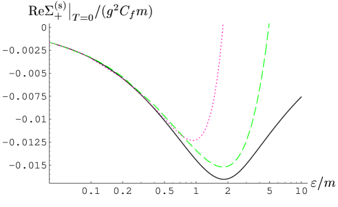
Figure 3.6: Exact expression for $\mathrm{Re}\Sigma_{+}^{\mathrm{(s)}}\big{|}_{T=0}$ (continuous curve) compared to two perturbative approximations (dashed curve: $\mathcal{O}(\varepsilon\log\varepsilon)$, dotted curve: $\mathcal{O}(\varepsilon^{3}\log\varepsilon)$).

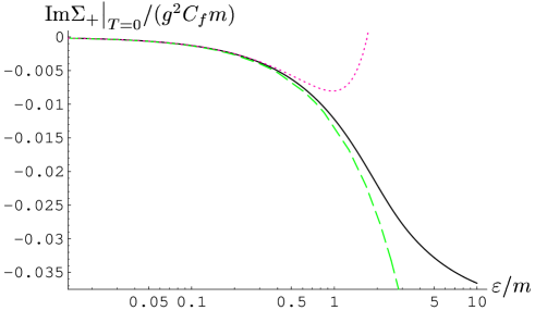
Figure 3.7: Exact expression for $\mathrm{Im}\Sigma_{+}\big{|}_{T=0}$ (continuous curve) compared to two perturbative approximations (dashed curve: $\mathcal{O}(\varepsilon)$, dotted curve: $\mathcal{O}(\varepsilon^{3})$).

Figure 3.8: $(v_{g}^{-1}-1)/(g^{2}C_{f})$ as a function of $\log_{10}((E-\mu)/m)$ at zero temperature (from [89]).

3.6 Fermi surface properties

The quasiparticle distribution function at zero temperature is given by

$$n(p)={1\over\pi}\int_{-\infty}^{\mu}dp_{0}\,\mathrm{Im}{1\over{-p_{0}+p+\Sigma_{+}(p_{0},p)-i\eta}}.$$ (3.104)

We are interested in the behavior of the distribution function for $p\sim\mu$. A possible non-regular behavior is expected from the singularity of the integrand. Thus we consider the quantity [90]

$$n^{\prime}(p):={1\over\pi}\int_{\mu-\delta}^{\mu}dp_{0}\,\mathrm{Im}{1\over{-p_{0}+p+\Sigma_{+}(p_{0},p)-i\eta}},$$ (3.105)

with $\delta\ll\mu$. We will neglect the imaginary part of the self energy in the following, since the imaginary part does not show a logarithmic enhancement in the vicinity of the Fermi surface. Thus we may write

$$n^{\prime}(p)\simeq\int_{\mu-\delta}^{\mu}dp_{0}\,\delta(p_{0}-p-\mathrm{Re}\Sigma_{+}(p_{0},p))=\int_{\mu-\delta}^{\mu}dp_{0}\,\delta(p_{0}-\bar{\omega}(p)){1\over 1-{\partial\mathrm{Re}\Sigma_{+}\over\partial p_{0}}},$$ (3.106)

where $\bar{\omega}(p)$ is the solution of the approximate dispersion law $p_{0}-p-\mathrm{Re}\Sigma_{+}=0$. We obtain

$$n^{\prime}(p)\simeq\Theta(\mu-\bar{\omega}(p)){1\over 1-{\partial\mathrm{Re}\Sigma_{+}\over\partial p_{0}}\big{|}_{p_{0}=\bar{\omega}(p)}}$$ (3.107)

The second factor on the right hand side is the group velocity. In contrast to a normal Fermi liquid it vanishes (like $1/\log|\bar{\omega}-\mu|$) for $\bar{\omega}\to\mu$. Therefore also the discontinuity at the Fermi surface vanishes. We remark that a similar behavior can also be found in condensed matter physics, in the context of high-$T_{c}$ superconductors. These systems have been termed “marginal Fermi liquids” [91].

Chapter 4 Anomalous specific heat at low temperature

4.1 General remarks

In this chapter we will continue our analysis of normal degenerate quark matter. We will compute the specific heat, which may be relevant for cooling of (proto-)neutron stars at temperatures above the color superconductivity phase transition. For a normal Fermi liquid (see Sec. 4.2) the specific heat is linear in the temperature for small temperatures. We will see, however, that the specific heat of cold dense quark matter contains an anomalous leading term of the order $T\log T$. As for the quark self energy, this logarithmic enhancement comes from long-range chromomagnetic fields. In this chapter we will also correct an error in a recent computation of the specific heat [92], which would have resulted in a $T^{3}\log T$ behavior of the specific heat at leading order.

4.2 Landau Fermi liquid theory

In this section we will give a brief account of Landau’s theory of Fermi liquids [93, 94], with particular emphasis on the specific heat. Our presentation follows closely Refs. [95, 96], to which we refer for further details.

To begin with, let us consider a uniform, non-relativistic gas of free spin-${1\over 2}$ fermions. The ground state consists of a Fermi sea, corresponding to the occupation number

$$n(k)=2\Theta(k_{F}-k),$$ (4.1)

where $k_{F}$ is the Fermi momentum. The total energy is given by

$$E=\sum_{\bf k}{k^{2}\over 2m}n(k).$$ (4.2)

Now let us turn on interactions between the particles adiabatically. We assume that the quantum mechanical states of the free system are gradually transformed into states of the interacting system. If this is the case, the interacting system is called a (Landau) Fermi liquid.

Next let us add an additional particle with momentum $k$ ($k>k_{F}$) to the free system, and then switch on the interactions. The eigenstate of the interacting system, which is obtained in this way, is called a quasiparticle. Denoting the energy of a quasiparticle with $\epsilon_{\bf k}$ and the chemical potential with $\mu$, one finds that the lifetime of quasiparticles is proportional to $(\epsilon_{\bf k}-\mu)^{-2}$ [96, 98] [see also Eq. (3.66) above]. Therefore the concept of a quasiparticle is well-defined in the vicinity of the Fermi surface. Since quasiparticles are adiabatically evolved from fermions, their distribution function at finite temperature is given by the usual Fermi-Dirac distribution,

$$n({\bf k})={1\over e^{(\epsilon_{\bf k}-\mu)/T}+1}.$$ (4.3)

A weak perturbation of the interacting system will induce a change $\delta n({\bf k})$ in the occupation number. Landau postulated that the change in the total energy of the system is then given by

$$\delta E=\sum_{\bf k}\epsilon^{0}_{\bf k}\delta n({\bf k})+{1\over 2}\sum_{{\bf k},{\bf k}^{\prime}}f({\bf k},{\bf k}^{\prime})\delta n({\bf k})\delta n({\bf k}^{\prime}),$$ (4.4)

where $\epsilon^{0}_{\bf k}$ is the energy of a quasiparticle, and $f({\bf k},{\bf k}^{\prime})$ is the quasiparticle interaction. For isotropic systems the effective mass $m^{*}$ is defined as

$${k_{F}\over m^{*}}={d\epsilon_{\bf k}^{0}\over dk}\bigg{|}_{k=k_{F}}.$$ (4.5)

The specific heat at constant volume and per unit volume is given by

$$\mathcal{C}_{v}={1\over V}\left({\partial E\over\partial T}\right)_{V}.$$ (4.6)

Using Eqs. (4.3)-(4.6) one finds that the specific heat of a Fermi liquid is linear in the temperature at low temperature (as for a free Fermi gas), $\mathcal{C}_{v}=\gamma T$, where the coefficient $\gamma$ is given by [96]

$$\gamma={1\over 3}m^{*}k_{F}.$$ (4.7)

Landau’s theory is corroborated by results of the microscopic theory, i.e. quantum field theory. For instance one finds also in quantum field theory that the specific heat of a cold fermionic system is linear in the temperature at leading order in many cases. The coefficient $\gamma$ can be computed e.g. from the 2PI effective action. For a theory with instantaneous four fermion interaction one finds [90]

$$\gamma={2\pi\over 3}\mathrm{Im}\sum_{\bf k}{\partial\over\partial\omega}\log\left(\epsilon_{\bf k}-\omega+\mathrm{Re}\Sigma_{\bf k}(\omega)+i\eta\right)\Big{|}_{\omega=\mu},$$ (4.8)

where $\Sigma_{\bf k}(\omega)$ is the fermion self energy. Evaluating the derivative with respect to $\omega$, one finds that the coefficient is proportional to the inverse group velocity,

$$v_{g}^{-1}=1-{\partial\mathrm{Re}\Sigma_{\bf k}\over\partial\omega}\bigg{|}_{\omega=\mu,\>k=\mathrm{on\>shell}}.$$ (4.9)

It is clear, however, that Eq. (4.8) becomes meaningless if the group velocity vanishes at $\omega=\mu$. In the previous chapter we did indeed encounter a situation where this happens, namely for a system with long-range interactions. In that case Landau’s theory is not applicable, and the leading term of the specific heat will not be linear in the temperature.

4.3 Specific heat from the entropy

The specific heat $\mathcal{C}_{v}$ at constant volume and per unit volume can be defined as the logarithmic derivative of the entropy density with respect to temperature at constant number density,

$$\mathcal{C}_{v}=T\left(\partial\mathcal{S}\over\partial T\right)_{\mathcal{N}},$$ (4.10)

This can be rewritten in terms of derivatives at constant $T$ or $\mu$ in the following way [99],

$${\cal C}_{v}=T\left[\left(\partial\mathcal{S}\over\partial T\right)_{\mu}-\left(\partial\mathcal{N}\over\partial T\right)_{\mu}^{2}\left(\partial\mathcal{N}\over\partial\mu\right)_{T}^{-1}\right],$$ (4.11)

At low temperatures only the term with the entropy contributes [100],

$$\mathcal{C}_{v}=T\left(\partial\mathcal{S}\over\partial T\right)_{\mu}+\mathcal{O}(T^{3}).$$ (4.12)

The thermodynamic potential for QCD is given by the following functional of the full propagators and self energies (assuming a ghost-free gauge) [101],

$$\beta\Omega[D,S]={1\over 2}\mathrm{Tr}\log D^{-1}-{1\over 2}\mathrm{Tr}\Pi D-\mathrm{Tr}\log S^{-1}+\mathrm{Tr}\Sigma S+\Phi[D,S],$$ (4.13)

where $S$ is the quark propagator, $\Sigma$ is the quark self energy, $D$ is the gluon propagator, $\Pi$ is the gluon self energy, and $\Phi$ is a series of 2-particle-irreducible (skeleton) diagrams.

Using the fact that $\Omega[D,S]$ is stationary with respect to variations of $D$ and $S$, one can derive an expression for the entropy which to two-loop order in the skeleton expansion is entirely given by propagators and self energies [24, 102]. We may neglect the contribution from longitudinal gluons, since they are subject to Debye screening and give therefore only a contribution to the normal Fermi liquid part of the entropy. Furthermore we may neglect antiparticle contributions in the fermionic sector since they would only lead to exponentially suppressed terms, $\propto\exp(-\mu/T)$. Thus we find for the entropy density (with $P=-\Omega/V$)

$$\!\!\!\!\!\!\!\!\!\mathcal{S}=\left(\partial P\over\partial T\right)_{\mu}\simeq-2N_{g}\int{d^{4}Q\over(2\pi)^{4}}{\partial n_{b}(q_{0})\over\partial T}\left(\mathrm{Im}\log D_{T}^{-1}-\mathrm{Im}\Pi_{T}\,\mathrm{Re}D_{T}\right)$$

$$\quad-4NN_{f}\int{d^{4}K\over(2\pi)^{4}}{\partial n_{f}(k_{0}-\mu)\over\partial T}\left(\mathrm{Im}\log S_{+}^{-1}-\mathrm{Im}\Sigma_{+}\,\mathrm{Re}S_{+}\right)+\mathcal{S}^{\prime},\qquad$$ (4.14)

where $D_{T}^{-1}=-q_{0}^{2}+q^{2}+\Pi_{T}$ and $S_{+}^{-1}=-k_{0}+k+\Sigma_{+}$ as in chapter 3. For the evaluation of the imaginary parts we always assume that $q_{0}$ and $k_{0}$ are replaced by $q_{0}+i\eta$ and $k_{0}+i\eta$, respectively [see Eqs. (A.9) and (A.12)].

In the original derivation of the anomalous specific heat in QED by Holstein et al. [103], only the term involving $\mathrm{Im}\log S_{+}^{-1}$ had been taken into account in the formula for the entropy density. While such a formula for the entropy density is known to be correct for standard Fermi liquid systems [90], it is not clear a priori how to justify it for more complicated systems, which possibly exhibit deviations from the Fermi liquid behavior. Therefore we will use the full expression (4.14) to calculate the entropy density at the order $g^{2}T\log T$ in the following. We will only neglect $\mathcal{S}^{\prime}$, since it vanishes at two-loop order [102, 24], and could therefore only give contributions which are suppressed by an additional factor of $g^{2}$.

4.3.1 Quark part

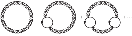
Figure 4.1: Sum of the gluon ring diagrams.

In Eq. (4.14) we have the following contribution from the quarks,

$$\mathcal{S}_{(\mathrm{q})}=-4NN_{f}\int{d^{4}K\over(2\pi)^{4}}{\partial n_{f}(k_{0}-\mu)\over\partial T}$$

$$\qquad\qquad\times\bigg{[}\mathrm{Im}\log\left(-k_{0}+k+\Sigma_{+}\right)-\mathrm{Im}\Sigma_{+}\,\mathrm{Re}{1\over-k_{0}+k+\Sigma_{+}}\bigg{]}$$

$$\,\qquad\simeq-{1\over\pi^{3}}NN_{f}\int_{0}^{\infty}dk\,k^{2}\int_{-\infty}^{\infty}dk_{0}{\partial n_{f}(k_{0}-\mu)\over\partial T}$$

$$\qquad\qquad\times\bigg{[}\mathrm{Im}\log\left(-k_{0}+k\right)+\mathrm{Re}\Sigma_{+}\,\mathrm{Im}{1\over-k_{0}+k}\bigg{]},\quad$$ (4.15)

where we have performed an expansion with respect to $\Sigma_{+}$, keeping only the free term and the term corresponding to a single quark self energy insertion. Diagrammatically, the latter part corresponds to the sum of the gluon ring diagrams, see Fig. 4.1. The free term gives the particle contribution to the free fermionic entropy density,

$$\mathcal{S}_{(\mathrm{q})}^{\mathrm{free}}\simeq NN_{f}{\mu^{2}T\over 3}.$$ (4.16)

In the last term in Eq. (4.15) the factor $\mathrm{Im}\,1/(-k_{0}+k)$ forces the self energy to be on the light cone. From Eq. (3.67) we obtain the following approximation of $\mathrm{Re}\Sigma_{+}$ at leading order

$$\mathrm{Re}\Sigma_{+}\simeq-{g^{2}C_{f}\over 12\pi^{2}}(k_{0}-\mu)\left[\log\left({M\over|k_{0}-\mu|}\right)+h\left({k_{0}-\mu\over T}\right)\right],$$ (4.17)

with $M\propto g_{\rm eff}\mu$, and $h$ is some function. From the Fermi-Dirac distribution in Eq. (4.15) we see that $k_{0}-\mu$ is of the order $T$. At leading logarithmic order we may therefore drop $h$ in Eq. (4.17), since it gives only a $\mathcal{O}(1)$ contribution to the result. This contribution would fix the scale under the logarithm, but this scale will be determined anyway in Sec. 4.5 using a slightly different approach. Thus we get

$$\mathcal{S}_{(\mathrm{q})}^{NLO}={N_{g}\over\pi^{2}}\int_{0}^{\infty}dk\,k^{2}{\partial n_{f}(k-\mu)\over\partial T}{g_{\rm eff}^{2}\over 12\pi^{2}}(k-\mu)\log\left({M\over|k-\mu|}\right).$$ (4.18)

We make the substitution $k=Tz+\mu$. The integral is dominated by small values of $z$, therefore we may send the lower integration limit to $-\infty$. Then we obtain at order $T\log T$

$$\mathcal{S}_{(\mathrm{q})}^{NLO}={g_{\rm eff}^{2}N_{g}\mu^{2}T\over 36\pi^{2}}\log\left({M\over T}\right).$$ (4.19)

This result agrees with the one of Holstein et al. [103] after correcting a factor of $4$ therein, as done previously in [104].

4.3.2 Gluon part

The gluon part $\mathcal{S}_{({\rm g})}$ is given by the first line of Eq. (4.14). It can again be interpreted in terms of ring diagrams, Fig. 4.1. Using the relation [24]

$$\mathrm{Im}\log D^{-1}=\arctan\left({\mathrm{Im}\Pi\over\mathrm{Re}D^{-1}}\right)-\pi\epsilon(q_{0})\theta\left(-\mathrm{Re}D^{-1}\right),$$ (4.20)

we write $\mathcal{S}_{({\rm g})}=\mathcal{S}_{(\mathrm{cut})}+\mathcal{S}_{(\Pi)}+\mathcal{S}_{(\mathrm{pole})}$, with

$$\mathcal{S}_{(\mathrm{cut})}=2N_{g}\int{d^{4}Q\over(2\pi)^{4}}{\partial n_{b}(q_{0})\over\partial T}\arctan\left({\mathrm{Im}\Pi_{T}\over q_{0}^{2}-q^{2}-\mathrm{Re}\Pi_{T}}\right),$$ (4.21)

$$\mathcal{S}_{(\Pi)}=-2N_{g}\int{d^{4}Q\over(2\pi)^{4}}{\partial n_{b}(q_{0})\over\partial T}\mathrm{Im}\Pi_{T}\,\mathrm{Re}{1\over q_{0}^{2}-q^{2}-\Pi_{T}},$$ (4.22)

$$\mathcal{S}_{(\mathrm{pole})}=2N_{g}\int{d^{4}Q\over(2\pi)^{4}}{\partial n_{b}(q_{0})\over\partial T}\pi\epsilon(q_{0})\theta\left(q_{0}^{2}-q^{2}-\mathrm{Re}\Pi_{T}\right).$$ (4.23)

For the cut term we use the approximation $q_{0}\ll q$, because it can be checked that including terms of higher order in $q_{0}$ would only produce terms of higher order than $T\log T$ (see Sec. 4.5). In this region we have from Eqs. (3.29) and (3.31)

$$\Pi_{T}\simeq-i{g_{\rm eff}^{2}\mu^{2}q_{0}\over 4\pi q}.$$ (4.24)

Introducing an UV-cutoff $q_{c}$ for the moment, we obtain

$$\mathcal{S}_{(\mathrm{cut})}\simeq{N_{g}\over 2\pi^{3}}\int_{-\infty}^{\infty}dq_{0}\int_{q_{0}}^{q_{c}}dq\,q^{2}\,{\partial n_{b}(q_{0})\over\partial T}\arctan\left({g_{\rm eff}^{2}\mu^{2}q_{0}\over 4\pi q^{3}}\right).$$ (4.25)

In order to evaluate this integral we make the substitution $y=q_{0}/T$, $x=4\pi q^{3}/(g_{\rm eff}^{2}\mu^{2}T)$. Keeping only the term of order $T\log T$, we get the (finite) result

$$\mathcal{S}_{(\mathrm{cut})}\simeq{g_{\rm eff}^{2}N_{g}\mu^{2}T\over 36\pi^{2}}\log\left(M^{\prime}\over T\right).$$ (4.26)

The determination of the constant $M^{\prime}$ would require a more accurate calculation including the longitudinal mode (see Sec. 4.5), which would show that $M^{\prime}\propto g_{\rm eff}\mu$.

Next let us evaluate $\mathcal{S}_{(\Pi)}$. Following similar steps as in the computation of $\mathcal{S}_{(\mathrm{cut})}$, we find

$$\mathcal{S}_{(\Pi)}\simeq 2N_{g}\int_{-\infty}^{\infty}{dq_{0}\over 2\pi}\int_{q_{0}}^{q_{c}}{dq\,q^{2}\over 2\pi^{2}}{\partial n_{b}(q_{0})\over\partial T}\left(-{g_{\rm eff}^{2}\mu^{2}q_{0}\over 4\pi q}\right){q^{2}\over q^{4}+\left({g_{\rm eff}^{2}\mu^{2}q_{0}\over 4\pi q}\right)^{2}}$$

$$\qquad\simeq-{g_{\rm eff}^{2}N_{g}\mu^{2}T\over 36\pi^{2}}\log\left(M^{\prime}\over T\right).$$ (4.27)

We observe that at order $T\log T$ this expression just cancels the contribution from Eq. (4.26).

Figure 4.2: Illustration of the inequality (4.31), with the plasma frequency $\omega_{p}$ normalized to $1$. Continuous line: $\omega_{T}(q)$, dashed line: $\Theta(\omega_{p}-q)+q\Theta(q-\omega_{p})$, dash-dotted line: $\omega_{p}+q$.

Finally let us consider the pole part. In the HDL approximation we have at low temperature $\mu{\partial\tilde{\Pi}_{T}\over\partial\mu}\simeq 2\tilde{\Pi}_{T}$, and therefore

$$\!\!\!\!\!\!\!\mu{\partial\mathcal{S}_{(\mathrm{pole})}\over\partial\mu}=-2N_{g}\int{d^{4}Q\over(2\pi)^{4}}{\partial n_{b}(q_{0})\over\partial T}\pi\epsilon(q_{0})\,\delta\left(q_{0}^{2}-q^{2}-\mathrm{Re}\tilde{\Pi}_{T}\right)2\,\mathrm{Re}\tilde{\Pi}_{T}$$

$$\,\quad\qquad=-4\pi N_{g}\int{d^{4}Q\over(2\pi)^{4}}{\partial n_{b}(q_{0})\over\partial T}(q_{0}^{2}-q^{2})\epsilon(q_{0})\,\delta\left(q_{0}^{2}-q^{2}-\mathrm{Re}\tilde{\Pi}_{T}\right),\qquad$$ (4.28)

where we have discarded contributions $\sim T^{3}$ which are negligible in the low-temperature limit. Using [76]

$$\epsilon(q_{0})\,\delta\left(\mathrm{Re}\tilde{D}_{T}^{-1}\right)=Z_{T}(q)\left(\delta(q_{0}-\omega_{T}(q))-\delta(q_{0}+\omega_{T}(q))\right)$$ (4.29)

we find

$$\mu{\partial\mathcal{S}_{(\mathrm{pole})}\over\partial\mu}=-{2N_{g}\over\pi^{2}}\int_{0}^{\infty}dq\,q^{2}{\partial n_{b}(\omega_{T}(q))\over\partial T}(\omega_{T}(q)^{2}-q^{2})Z_{T}(q).$$ (4.30)

We would like to give an estimate for this integral. With the plasma frequency $\omega_{p}=g_{\rm eff}\mu/(\pi\sqrt{3})$ we have the inequalities

$$\Theta(\omega_{p}-q)+q\Theta(q-\omega_{p})<\omega_{T}(q)<\omega_{p}+q$$ (4.31)

(see Fig. 4.2), and

$$Z_{T}(q)<{1\over 2q}$$ (4.32)

(see Fig. B.2). Since we assume $T\ll\omega_{p}\propto g_{\rm eff}\mu$, we can therefore estimate

$$\int_{0}^{\infty}dq\,q^{4}{\partial n_{b}(\omega_{T}(q))\over\partial T}Z_{T}(q)<\int_{0}^{\infty}dq\,q^{4}{\partial n_{b}(\omega_{T}(q))\over\partial T}{1\over 2q}$$

$$\qquad<{1\over 2}\int_{0}^{\omega_{p}}dq\,q^{3}{\partial n_{b}(\omega_{p})\over\partial T}+{1\over 2}\int_{\omega_{p}}^{\infty}dq\,q^{3}{\partial n_{b}(q)\over\partial T}\simeq{\omega_{p}^{5}\over 8T^{2}}e^{-\omega_{p}/T},\qquad\qquad$$ (4.33)

and

$$\int_{0}^{\infty}dq\,q^{2}{\partial n_{b}(\omega_{T}(q))\over\partial T}\omega_{T}(q)^{2}Z_{T}(q)<\int_{0}^{\infty}dq\,q^{2}{\partial n_{b}(\omega_{T}(q))\over\partial T}(\omega_{p}+q)^{2}{1\over 2q}$$

$$\qquad<{1\over 2}\int_{0}^{\omega_{p}}dq\,q(\omega_{p}+q)^{2}{\partial n_{b}(\omega_{p})\over\partial T}+{1\over 2}\int_{\omega_{p}}^{\infty}dq\,q(\omega_{p}+q)^{2}{\partial n_{b}(q)\over\partial T}$$

$$\qquad\simeq{17\omega_{p}^{5}\over 24T^{2}}e^{-\omega_{p}/T}.$$ (4.34)

Apart from terms $\sim T^{3}$ which are dropped in the derivative with respect to $\mu$, this crude estimate (which we shall refine in Sec. 4.5.5) shows that the pole contribution is exponentially suppressed (essentially because of $\omega_{T}\geq\omega_{p}$).

4.3.3 Result

From the previous subsections we find the following result for the entropy density at low temperature,

$$\mathcal{S}=\mathcal{S}_{(\mathrm{g})}+\mathcal{S}_{(\mathrm{q})}\simeq NN_{f}{\mu^{2}T\over 3}+{g_{\rm eff}^{2}N_{g}\mu^{2}T\over 36\pi^{2}}\log\left({M\over T}\right).$$ (4.35)

From Eq. (4.26) we see that the $T\log T$ term can also be obtained by starting only with

$$\mathcal{S}\simeq NN_{f}{\mu^{2}T\over 3}-2N_{g}\int{d^{4}Q\over(2\pi)^{4}}{\partial n_{b}(q_{0})\over\partial T}\mathrm{Im}\log D_{T}^{-1}.$$ (4.36)

This formula corresponds to integrating out the fermions, as has indeed been done in the approach of [100, 105]. On the other hand, we see from Eqs. (4.15) and (4.19) that one also gets the correct result by using the purely fermionic expression

$$\mathcal{S}\simeq-4NN_{f}\int{d^{4}K\over(2\pi)^{4}}{\partial n_{f}(k_{0}-\mu)\over\partial T}\mathrm{Im}\log(-k_{0}+k+\mathrm{Re}\Sigma_{+}),$$ (4.37)

which justifies the starting point of [103].

4.3.4 A note on the Sommerfeld expansion

Since the inverse group velocity diverges on the Fermi surface, one might wonder whether the coefficient of the linear power of temperature in the specific heat should also diverge. Of course we have seen from explicit calculations that this is not the case. In order to see in which way a straightforward application of Fermi liquid techniques goes wrong in our case, let us consider again the entropy density. From Eq. (4.15) we have

$$\mathcal{S}^{NLO}=-{1\over\pi^{2}}NN_{f}\int_{0}^{\infty}dk_{0}\,k_{0}^{2}{\partial n_{f}(k_{0}-\mu)\over\partial T}\mathrm{Re}\Sigma_{+}|_{T=0}.$$ (4.38)

A naive Sommerfeld expansion, assuming (erroneously) that $\mathrm{Re}\Sigma_{+}|_{T=0}$ is analytic at $k_{0}=\mu$, would lead to

$$\mathcal{S}^{NLO}\simeq-NN_{f}{T\over 3}{\partial\over\partial k_{0}}\left(k_{0}^{2}\mathrm{Re}\Sigma_{+}\right)\Big{|}_{T=0,\,k_{0}=\mu}={\rm"}g^{2}\mu^{2}T\times\infty{\rm"}.$$ (4.39)

Then we would have for the part of the entropy density which is linear in temperature

$$\mathcal{S}_{lin.}\sim NN_{f}{\mu^{2}T\over 3}(1+{\rm"}g^{2}\infty{\rm"}),$$ (4.40)

Of course this equation is wrong, since the assumption that $\mathrm{Re}\Sigma_{+}|_{T=0}$ is analytic at $k_{0}=\mu$ is incorrect. The explicit calculation (see above) shows that instead of a linear term with a singular coefficient, one obtains a $T\log T$ term with a finite coefficient.

4.4 Specific heat from the energy density

The energy density can be obtained from the expectation value of the energy momentum tensor,

$$\mathcal{U}={1\over V}\int d^{3}x\,\langle T^{00}(x)\rangle,$$ (4.41)

and the specific heat is then given by

$$\mathcal{C}_{v}=\left({d\mathcal{U}\over dT}\right)_{\mathcal{N}}.$$ (4.42)

Here the temperature derivative has to be taken at constant particle number density, in contrast to the calculation of the low temperature specific heat in the previous section, where all temperature derivatives had to be taken at constant chemical potential, see Eqs. (4.12), (4.14). Of course, both methods will ultimately yield the same result.

In [92] the specific heat is computed using the following formula for the total energy density,

$$\mathcal{U}=2\int dk_{0}\int{d^{3}k\over(2\pi)^{3}}n_{f}(k_{0}-\mu)\,k_{0}\,\rho_{+}(k_{0},k),$$ (4.43)

where $\rho_{+}$ is the spectral density of the positive energy component of the quark propagator (see below). It should be noted that this formula is incorrect even for a theory with only instantaneous interactions of the type

$$H_{int}={1\over 2}\int d^{3}x\,d^{3}x^{\prime}\,\psi_{\alpha}^{\dagger}({\bf x},t)\psi_{\beta}^{\dagger}({\bf x^{\prime}},t)V_{\alpha\alpha^{\prime},\beta\beta^{\prime}}({\bf x}-{\bf x^{\prime}})\psi_{\beta^{\prime}}({\bf x^{\prime}},t)\psi_{\alpha^{\prime}}({\bf x},t),$$ (4.44)

in which case the correct formula reads [106]

$$\mathcal{U}=2\int dk_{0}\int{d^{3}k\over(2\pi)^{3}}n_{f}(k_{0}-\mu)\,{1\over 2}(k_{0}+k)\rho_{+}(k_{0},k).$$ (4.45)

The anomalous behavior of the specific heat comes from dynamically screened interactions, whose non-instantaneous character cannot be neglected. It would be rather difficult to generalize Eq. (4.45) directly for non-instantaneous interactions, because one would have to use an effective Hamiltonian which is nonlocal in time. If one naively tries to compute the anomalous specific heat from Eq. (4.45), the coefficient of the logarithmic term turns out to be wrong by a factor ${1\over 2}$. Therefore, we will follow a slightly different approach, using the energy momentum tensor of QCD without integrating out the gluons.

The energy momentum tensor can be written as a sum of three pieces,

$$T^{\mu\nu}=T^{\mu\nu}_{(\mathrm{q})}+T^{\mu\nu}_{(\rm{g})}+T^{\mu\nu}_{(\mathrm{int.})},$$ (4.46)

corresponding to the quark part, the gluon part, and the interaction part. The contributions of these parts will be evaluated in the following subsections. We will neglect gluon self interactions and ghost contributions, since they give only higher order corrections at low temperature.

4.4.1 Quark part

The quark part is given by

$$T^{00}_{(\mathrm{q})}=i\sum_{f}\bar{\psi}_{f}\gamma^{0}\partial^{0}\psi_{f},$$ (4.47)

where we have written explicitly the sum over flavor space. This is the (only) contribution which is taken into account by Boyanovsky and de Vega [92]. Let us repeat their calculation, but for simplicity without the renormalization group improvement of the quark propagator proposed in [107]. As for the entropy density is is sufficient to take into account only the positive energy component of the quark propagator. Thus we find

$$\mathcal{U}_{(\mathrm{q})}=2NN_{f}\int dk_{0}\int{d^{3}k\over(2\pi)^{3}}n_{f}(k_{0}-\mu)\,k_{0}\,\rho_{+}(k_{0},k),$$ (4.48)

where the spectral density is defined as $\rho_{+}\equiv{1\over\pi}\mathrm{Im}S_{+}$.

In order to obtain the specific heat from Eq. (4.42), we have to determine first the temperature dependence of the chemical potential from the condition

$${d\mathcal{N}\over dT}\equiv{\partial\mathcal{N}\over\partial T}+{d\mu\over dT}{\partial\mathcal{N}\over\partial\mu}=0,$$ (4.49)

where the particle number density $\mathcal{N}$ is given by

$$\mathcal{N}=2NN_{f}\int dk_{0}\int{d^{3}k\over(2\pi)^{3}}n_{f}(k_{0}-\mu)\,\rho_{+}(k_{0},k)$$ (4.50)

(up to anti-particle contributions). We expand $\mathcal{N}$ with respect to $g$,

$$\mathcal{N}=\mathcal{N}_{0}+g_{\rm eff}^{2}\mathcal{N}_{2}+\ldots$$ (4.51)

The free contribution $\mathcal{N}_{0}$ is given by

$$\mathcal{N}_{0}=NN_{f}\left({\mu^{3}\over 3\pi^{2}}+{\mu T^{2}\over 3}\right).$$ (4.52)

In $\mathcal{N}_{2}$ we are only interested in contributions which contain $\log(M/T)$. Such terms arise from infrared singularities from the gluon propagator, which are dynamically screened. This corresponds to scattering processes of quarks which are close to the Fermi surface. Therefore the anomalous terms come from the region $k\sim k_{0}\sim\mu$, where $\Sigma_{+}$ is given by (4.17) at leading order. At leading logarithmic order we may again neglect the function $h$ in Eq. (4.17). Subtracting the temperature independent part, we find then

$$g_{\rm eff}^{2}\mathcal{N}_{2}=2NN_{f}\int dk_{0}\int{d^{3}k\over(2\pi)^{3}}\left(n_{f}(k_{0}-\mu)-\Theta(\mu-k_{0})\right)\delta(k_{0}-k-\mathrm{Re}\Sigma_{+})\bigg{|}_{\mathcal{O}(g_{\rm eff}^{2})},$$ (4.53)

where we have approximated the spectral density with a delta function, since the imaginary part of $\Sigma_{+}$ is negligible compared to its real part. The integration can be performed easily, with the result

$$g_{\rm eff}^{2}\mathcal{N}_{2}\simeq{g_{\rm eff}^{2}N_{g}\mu T^{2}\over 36\pi^{2}}\log\left(M\over T\right).$$ (4.54)

We notice that this result is consistent with the result for the entropy density, Eq. (4.35). Now we can solve Eq. (4.49) at low temperature,

$${d\mu\over dT}=-{2\pi^{2}T\over 3\mu}-{g^{2}C_{f}T\over 18\mu}\log\left(M\over T\right).$$ (4.55)

The approximate solution to this differential equation is given by

$$\mu(T)\simeq\mu(0)\left(1-{\pi^{2}T^{2}\over 3\mu(0)^{2}}-{g^{2}C_{f}T^{2}\over 36\mu(0)^{2}}\log\left({M\over T}\right)\right).$$ (4.56)

Eqs. (4.55) and (4.56) correctly reproduce the beginning of the perturbative expansions of Eqs. (2.37) and (2.38) in Ref. [92].

For the specific heat we obtain from Eq. (4.48), following the same steps as in the calculation of $d\mathcal{N}/dT$,

$$\mathcal{C}_{v(\mathrm{q})}\simeq NN_{f}\mu^{2}T+NN_{f}{\mu^{3}\over\pi^{2}}{d\mu\over dT}+{g_{\rm eff}^{2}N_{g}\mu^{2}T\over 18\pi^{2}}\log\left({M\over T}\right).$$ (4.57)

Using Eqs. (4.55) and (4.56) we find that the $T\log T$-terms cancel,

$$\mathcal{C}_{v(\mathrm{q})}\simeq NN_{f}{\mu^{2}T\over 3},$$ (4.58)

as stated in [92]. We should emphasize that this cancellation has nothing to do with the nonperturbative renormalization group method which is employed in [92]. It should also be noted that this renormalization group method has been criticized recently [108], because the neglect of the $\beta$-function in the renormalization group equation used in [92, 107] does not seem to be justified.

4.4.2 Gluon part

We now turn to the gluon part of the energy density, which has been explicitly neglected in Ref. [92]. This is given by

$$T^{00}_{({\rm g})}={1\over 2}\left({\bf E}^{a}\cdot{\bf E}^{a}+{\bf B}^{a}\cdot{\bf B}^{a}\right).$$ (4.59)

Neglecting gluon self interactions, and keeping only the transverse part of the gluon propagator, we obtain

$$\mathcal{U}_{({\rm g})}\simeq 2N_{g}\int{d^{4}Q\over(2\pi)^{4}}n_{b}(q_{0})\,\mathrm{Im}\left(\left(q_{0}^{2}+q^{2}\right)D_{T}\right).$$ (4.60)

The pole contribution to this integral is again exponentially suppressed, therefore we only have to consider the cut contribution. At low temperature we may neglect the temperature dependence of the gluon self energy. Subtracting a less infrared sensitive contribution not involving the Bose distribution (corresponding to the non-$n_{b}$-part in Sec. 4.5), we find

$$\mathcal{U}_{({\rm g})}\simeq 2N_{g}\int{d^{4}Q\over(2\pi)^{4}}\left(n_{b}(q_{0})+\Theta(-q_{0})\right)(q_{0}^{2}+q^{2}){{g_{\rm eff}^{2}\mu^{2}q_{0}\over 4\pi q}\over\left(q_{0}^{2}-q^{2}\right)^{2}+\left({g_{\rm eff}^{2}\mu^{2}q_{0}\over 4\pi q}\right)^{2}}.$$ (4.61)

After the substitution $q_{0}=Ty$, $q^{3}=g_{\rm eff}^{2}\mu^{2}Tx/(4\pi)$ the integral can be readily done, with the result

$$\mathcal{U}_{({\rm g})}\simeq{g_{\rm eff}^{2}N_{g}\mu^{2}T^{2}\over 72\pi^{2}}\log(M/T),$$ (4.62)

which gives the following contribution to the specific heat at order $T\log T$,

$$\mathcal{C}_{v({\rm g})}\simeq{g_{\rm eff}^{2}N_{g}\mu^{2}T\over 36\pi^{2}}\log(M/T).$$ (4.63)

Again the determination of the constant $M$ would require a more accurate calculation, similar to the one in Sec. 4.5.

4.4.3 Interaction part

The interaction part is given by

$$T^{00}_{(\mathrm{int})}=g\sum_{f}\bar{\psi}_{f}\gamma^{0}A^{0}_{a}T_{a}\psi_{f}.$$ (4.64)

The expectation value of this term is essentially given by the resummed gluon ring diagram as in Fig. 4.1. However, here only the longitudinal component of the gluon propagator appears in the loop. This mode is subject to Debye screening, so it can contribute only to the normal Fermi liquid part of the specific heat.

4.4.4 Result

From the previous subsections we see that the only contribution to the specific heat at order $g^{2}T\log T$ when calculated along the lines of Ref. [92] comes from the gluon part, Eq. (4.63). While this confirms the observation of Ref. [92] that the quark contribution of order $g^{2}T\log T$ cancels against a similar term from the temperature dependence of the chemical potential at fixed number density, it shows that the neglect of the gluon contribution to the energy density in [92] is not justified.

Our result for the specific heat from the energy density is consistent with the result for the entropy density in Sec. 4.4. For the entropy density we found at leading logarithmic order that it was sufficient to take into account only the contribution of fermionic quasiparticles. For the energy density, on the other hand, the purely fermionic formula (4.48) is not sufficient to give the correct result.

4.5 Higher orders in the specific heat

In this section we will evaluate higher terms in the low temperature specific heat which go beyond the leading logarithmic approximation. A convenient starting point is the following expression for the pressure, which becomes exact in the limit of large flavor number $N_{f}$ [109, 110, 111],

$$\!\!\!\!\!\!\!\!\!\!\!\!P=NN_{f}\left({\mu^{4}\over 12\pi^{2}}+{\mu^{2}T^{2}\over 6}+{7\pi^{2}T^{4}\over 180}\right)$$

$$-N_{g}\int{d^{3}q\over(2\pi)^{3}}\int_{0}^{\infty}{dq_{0}\over\pi}\bigg{[}2\left([n_{b}(q_{0})+{1\over 2}]\mathrm{Im}\log D_{T}^{-1}-{1\over 2}\mathrm{Im}\log D_{\rm vac}^{-1}\right)$$

$$\quad+\left([n_{b}(q_{0})+{1\over 2}]\mathrm{Im}\log{D_{L}^{-1}\over q^{2}-q_{0}^{2}}-{1\over 2}\mathrm{Im}\log{D_{\rm vac}^{-1}\over q^{2}-q_{0}^{2}}\right)\bigg{]}+{\cal O}(g^{4}\mu^{4}),$$ (4.65)

where the inverse gauge boson propagators are given by $D_{T}^{-1}=q^{2}-q_{0}^{2}+\Pi_{T}+\Pi_{\rm vac}$, $D_{L}^{-1}=q^{2}-q_{0}^{2}+\Pi_{L}+\Pi_{\rm vac}$, and $D_{\rm vac}^{-1}=q^{2}-q_{0}^{2}+\Pi_{\rm vac}$. The first line of Eq. (4.65) is simply the pressure of a free fermionic quantum gas, and the remaining part is essentially given by the sum of gluon ring diagrams in Fig. 4.1. At finite $N_{f}$, Eq. (4.65) with $\Pi$ including also the leading contributions from gluon loops still collects all infrared-sensitive contributions up to and including three-loop order [112, 113]. We shall however find that all contributions from gluon loops to $\Pi$ are suppressed with $(T/\mu)^{2}$ in the specific heat, and will thus be negligible for $T\ll\mu$ compared to the terms we shall keep.

In the following we will always drop temperature independent terms in the pressure, since they do not contribute to the specific heat at low temperature. We will refer to terms involving the bosonic distribution function $n_{b}$ as “$n_{b}$-parts”, and to the remaining ones as “non-$n_{b}$-parts”.

From the explicit form of the self energy (see Sec. 3.2 and [77]) we see that the $q$-integration naturally splits into three regions: $q<q_{0}$, $q_{0}<q<2\mu-q_{0}$, and $2\mu-q_{0}<q<2\mu+q_{0}$. We will consider these regions separately in the following.

4.5.1 Transverse contribution, region II

The $n_{b}$-part of the contribution of the transverse gluons to the pressure is given by

$${P_{T}\over N_{g}}=-2\int{d^{3}q\over(2\pi)^{3}}\int_{0}^{\infty}{dq_{0}\over\pi}\,n_{b}(q_{0})\mathrm{Im}\log(q^{2}-q_{0}^{2}+\Pi_{T}+\Pi_{\rm vac}).$$ (4.66)

The cut contribution from region II is given by

$${P_{T}^{\mathrm{II}}\over N_{g}}=-2\int_{0}^{\infty}{dq_{0}\over\pi}\int_{q_{0}}^{2\mu-q_{0}}{dq\,q^{2}\over 2\pi^{2}}\,n_{b}(q_{0})\arctan{\mathrm{Im}\Pi_{T}\over q^{2}-q_{0}^{2}+\mathrm{Re}\Pi_{T}+\mathrm{Re}\Pi_{\rm vac}}.$$ (4.67)

As long as $T\ll\mu$ it is sufficient to take the self energy at zero temperature.

The Bose-Einstein factor and the leading term in the gluon self energy set the characteristic scales,

$$q_{0}\sim T,\qquad q\sim(g_{\rm eff}^{2}\mu^{2}T)^{1/3}.$$ (4.68)

We want to perform an expansion with respect to a parameter $b$ defined as

$$b:=\left({T\over g_{\rm eff}\mu}\right)^{1/3}.$$ (4.69)

It turns out that the following approximation of the gluon self energy is sufficient through order $T^{3}\log T$ in the entropy density,

$$\mathrm{Re}\Pi_{T}(q_{0},q)\simeq{g_{\rm eff}^{2}\over\pi^{2}}\left({\mu^{2}q_{0}^{2}\over q^{2}}-{\mu^{2}q_{0}^{4}\over 3q^{4}}\right),$$ (4.70)

$$\mathrm{Im}\Pi_{T}(q_{0},q)\simeq{g_{\rm eff}^{2}\over 4\pi}\left(-{\mu^{2}q_{0}\over q}+{\mu^{2}q_{0}^{3}\over q^{3}}-{qq_{0}\over 4}\right).$$ (4.71)

The first two terms in both lines are the leading terms of an expansion of the HDL self energy in powers of $q_{0}$. Naively counting powers of $b$ in the integrand one would conclude that only these terms are responsible for the coefficients of the expansion in $b$, while the other terms in the self energy should give only terms which are suppressed with additional powers of $g$ in the pressure. In principle this is correct, but it turns out that it is necessary to keep also the last term in Eq. (4.71), which is beyond the HDL approximation. As we well see in Sec. 4.5.3 this term gives a contribution in the hard region, where the approximation $q\ll\mu$ is not justified.

Introducing dimensionless integration variables $x$ and $y$ via

$$q_{0}=b^{3}g_{\rm eff}\mu y,\quad q=bg_{\rm eff}\mu(x/(4\pi))^{1/3},$$ (4.72)

we find after expanding the integrand with respect to $b$,

$${P_{T}^{\mathrm{II}}\over N_{g}}\simeq{g_{\rm eff}^{4}\mu^{4}\over 12\pi^{4}}\int_{0}^{\infty}dy{1\over e^{y}-1}\int_{x_{min}}^{x_{max}}dx\bigg{[}b^{6}\arctan\left({y\over x}\right)$$

$$+{y(g_{\rm eff}^{2}x^{2}-64y^{2})\over 8(2\pi^{2}x)^{1/3}(x^{2}+y^{2})}b^{8}+{32(2x)^{1/3}y^{5}\over\pi^{4/3}(x^{2}+y^{2})^{2}}b^{10}$$

$$-{32y^{5}(24x^{2}y^{2}-8y^{4}+\pi^{2}(x^{2}+y^{2})^{2})\over 3\pi^{2}x(x^{2}+y^{2})^{3}}b^{12}+{\cal O}(b^{14})\bigg{]},$$ (4.73)

with $x_{min}=4\pi b^{6}y^{3}$ and $x_{max}=4\pi(2-b^{3}g_{\rm eff}y)^{3}/(bg_{\rm eff})^{3}$. In the coefficients of this expansion we have written down only those terms which do not ultimately lead to terms that are suppressed by explicit positive powers of $g_{\rm eff}$. The integrations are now straightforward, and we find

$$\!\!\!\!\!\!\!\!\!{P_{T}^{\mathrm{II}}\over N_{g}}\simeq g_{\rm eff}^{4}\mu^{4}\bigg{[}{b^{6}\over 72\pi^{2}}\left(\log\left({32\pi\over(bg_{\rm eff})^{3}}\right)+\gamma_{E}-{6\over\pi^{2}}\zeta^{\prime}(2)+{3\over 2}\right)-{2^{2/3}\Gamma\left({8\over 3}\right)\zeta\left({8\over 3}\right)\over 3\sqrt{3}\pi^{11/3}}b^{8}$$

$$\quad+{8\,2^{1/3}\Gamma\left({10\over 3}\right)\zeta\left({10\over 3}\right)\over 9\sqrt{3}\pi^{13/3}}b^{10}+{16(\pi^{2}-8)\over 45\pi^{2}}b^{12}\log b+\tilde{c}_{T}b^{12}+\mathcal{O}(b^{14})\bigg{]}.$$ (4.74)

The evaluation of the constant $\tilde{c}_{T}$ is a bit more involved because one has to sum up an infinite series of contributions from the infrared region. This will be done in Sec. 4.5.7.

4.5.2 Longitudinal contribution, region II

The $n_{b}$-part of the contribution of the longitudinal gluons to the pressure is given by

$${P_{L}\over N_{g}}=-\int{d^{3}q\over(2\pi)^{3}}\int_{0}^{\infty}{dq_{0}\over\pi}\,n_{b}(q_{0})\mathrm{Im}\log\left({q^{2}-q_{0}^{2}+\Pi_{L}+\Pi_{\rm vac}\over q^{2}-q_{0}^{2}}\right).$$ (4.75)

As in the previous section the $q$-integration decomposes into three parts. In the second region ($q_{0}<q<2\mu-q_{0}$) the characteristic scales are now

$$q_{0}\sim T,\qquad q\sim g_{\rm eff}\mu.$$ (4.76)

In a similar way as in the previous section, the gluon self energy can be approximated as

$$\mathrm{Re}\Pi_{L}(q_{0},q)\simeq{g_{\rm eff}^{2}\over\pi^{2}}\left(\mu^{2}-{2\mu^{2}q_{0}^{2}\over q^{2}}\right),$$ (4.77)

$$\mathrm{Im}\Pi_{L}(q_{0},q)\simeq{g_{\rm eff}^{2}\over 2\pi}\left({\mu^{2}q_{0}\over q}-{\mu^{2}q_{0}^{3}\over q^{3}}-{qq_{0}\over 4}\right).$$ (4.78)

We introduce dimensionless integration variables $y$ and $z$ via

$$q_{0}=b^{3}g_{\rm eff}\mu y,\quad q=g_{\rm eff}\mu z/\pi.$$ (4.79)

Then we find after expanding the integrand with respect to $b$,

$$\!\!\!\!\!\!\!\!\!\!\!\!\!\!\!\!\!{P_{L}^{\mathrm{II}}\over N_{g}}\simeq{g_{\rm eff}^{4}\mu^{4}\over 16\pi^{2}}\int_{0}^{\infty}dy{1\over e^{y}-1}\int_{z_{min}}^{z_{max}}dz$$

$$\!\!\!\!\!\!\!\!\!\!\!\!\!\!\!\!\!\times\bigg{[}b^{6}{yz(-4\pi^{2}(1+z^{2})+g_{\rm eff}^{2}z^{4})\over\pi^{4}(1+z^{2})^{2}}+b^{12}{y^{3}(\pi^{2}-12(z^{2}+1))\over 3z(1+z^{2})^{3}}+{\cal O}(b^{18})\bigg{]},\quad$$ (4.80)

with $z_{min}=b^{3}y\pi$ and $z_{max}=(2/g_{\rm eff}-b^{3}y)\pi$. In the coefficients of this expansion we have written down only those terms which do not ultimately lead to terms that are suppressed by explicit positive powers of $g_{\rm eff}$. The integrations are now straightforward, and we find

$${P_{L}^{\mathrm{II}}\over N_{g}}\simeq g_{\rm eff}^{4}\mu^{4}\Bigg{[}{b^{6}\over 48\pi^{2}}\left(1+\log\left({g_{\rm eff}^{2}\over 4\pi^{2}}\right)\right)$$

$$\qquad\quad+{\pi^{2}(12-\pi^{2})\over 240}b^{12}\log b+\tilde{c}_{L}b^{12}+\mathcal{O}(b^{18}\log b)\Bigg{]}.$$ (4.81)

As in the transverse sector, the determination of the constant $\tilde{c}_{L}$ requires summation of contributions from the infrared region, which will be done in Sec. 4.5.7.

4.5.3 Contributions from the upper integration limit

In this subsection we will show that the HDL approximation for the gluon self energy is sufficient to produce the series in $b$, apart from the order $b^{6}$, where precisely two additional terms in the gluon the self energy are necessary, one in the transverse part and one in the longitudinal part.

First let us focus on the transverse part. It is convenient to multiply the denominator and the numerator of the argument of the arctangent in Eq. (4.67) with a factor $x^{1/3}/(g_{\rm eff}^{2}\mu^{2}b^{2})$. Dropping numerical factors, and also powers of $y$, we have then the following effective power counting rules:

$$\!\!\!q^{2}\!\!\! \to \!\!\!x,$$ (4.82)

$$\!\!\!q_{0}^{2}\!\!\! \to \!\!\!x^{1/3}b^{4},$$ (4.83)

$$\!\!\!g_{\rm eff}^{2}\mu^{2}\left({q_{0}\over q}\right)^{n}\!\!\! \to \!\!\!\left({b^{2}\over x^{1/3}}\right)^{n-1},$$ (4.84)

$$\!\!\!g_{\rm eff}^{2}\mu^{2}\left({q_{0}\over q}\right)^{n}\left({q\over\mu}\right)^{r}\left({q_{0}\over\mu}\right)^{s}\left({T\over\mu}\right)^{2t}\!\!\! \to \!\!\!\left({b^{2}\over x^{1/3}}\right)^{n-1+{r+3s+6t\over 2}}\left(g_{\rm eff}^{2}x\right)^{r+s+2t\over 2},\qquad$$ (4.85)

where $n,r,s,t\in\mathbbm{N}_{0}$. Here the third line corresponds to a HDL contribution, and the last line corresponds to terms beyond the HDL approximation. At first sight, we would expect that contributions from the last line (when $r+s+t>0$) could only produce terms which are suppressed with powers of $g_{\rm eff}$ in the pressure. A more careful analysis is required, however, since the upper integration limit is proportional to $1/g_{\rm eff}^{3}$, which might invalidate the naive power counting in the integrand.

After the Taylor expansion with respect to $b$, the term of order $b^{6+2M}$ in the integrand will have the following general structure for $M\geq 1$,

$$g_{\rm eff}^{4}\mu^{4}b^{6}{\mathsf{P}_{2M}\over(x^{2}+y^{2})^{M}},$$ (4.86)

where $\mathsf{P}_{2M}$ is of the order $b^{2M}$. We note that $\mathsf{P}_{2M}$ is a polynomial of degree $2M$ in the expressions on the right hand sides of Eqs. (4.82)-(4.85). This can be seen from expanding first $\mathrm{Re}\Pi_{T}$ and $\mathrm{Im}\Pi_{T}$, and then the arctangent, with respect to $b$. Each term in this polynomial contains at least one factor which comes from $\mathrm{Im}\Pi_{T}$, and at least one factor which comes from $q^{2}-q_{0}^{2}+\mathrm{Re}\Pi_{T}$. Explicitly, we find contributions to the pressure of the following type from the region of large $x$ in (4.86),

$$U_{M}:=g_{\rm eff}^{4}\mu^{4}\int^{1/(bg_{\rm eff})^{3}}dx{b^{6+2M}\over x^{2M}}x^{\alpha+{\beta\over 3}}\prod_{i=1}^{\gamma}x^{-{c_{i}\over 3}}(g_{\rm eff}^{2}x)^{d_{i}}\prod_{j=1}^{\delta}x^{-{e_{j}\over 3}}(g_{\rm eff}^{2}x)^{f_{j}},$$ (4.87)

where $x^{\alpha+{\beta\over 3}}$ comes from the free gluon propagator, the first product comes from $\mathrm{Re}\Pi_{T}$, and the second one from $\mathrm{Im}\Pi_{T}$. The parameters $\alpha$, $\beta$, $\gamma$, $\delta$, $c_{i}$, $d_{i}$, $e_{j}$, and $f_{j}$ are natural numbers (including zero). The properties of $\mathsf{P}_{2M}$ listed above lead to the following set of restrictions for these parameters,

$$4\beta+2\sum_{i=1}^{\gamma}c_{i}+2\sum_{j=1}^{\delta}e_{j} = 2M,$$ (4.88)

$$\alpha+\beta+\gamma+\delta = 2M,$$ (4.89)

$$\alpha+\beta+\gamma \geq 1,$$ (4.90)

$$\delta \geq 1.$$ (4.91)

We can eliminate $\alpha$ and $\beta$ in Eq. (4.87) with the help of Eqs. (4.88) and (4.89). After performing the integration we obtain

$$U_{M}\sim b^{v}g_{\rm eff}^{w},$$ (4.92)

where the exponents are given by

$$v=3\Big{(}1+M+\gamma+\delta-\sum_{i=1}^{\gamma}d_{i}-\sum_{j=1}^{\delta}f_{j}\Big{)},$$ (4.93)

$$w=-3+M+3\gamma+3\delta-\sum_{i=1}^{\gamma}d_{i}-\sum_{j=1}^{\delta}f_{j}.$$ (4.94)

We are interested in contributions with $w\leq 0$. Therefore we obtain from (4.91) and (4.94)

$${1\over 3}\Big{(}3-M-3\gamma+\sum_{i=1}^{\gamma}d_{i}+\sum_{j=1}^{\delta}f_{j}\Big{)}\geq\delta\geq 1.$$ (4.95)

Furthermore we get from $\beta\geq 0$ using Eq. (4.88)

$$M-\sum_{i=1}^{\gamma}c_{i}-\sum_{j=1}^{\delta}e_{j}\geq 0.$$ (4.96)

Combining the inequalities (4.95) and (4.96) we get

$$3\gamma+\sum_{i=1}^{\gamma}(c_{i}-d_{i})+\sum_{j=1}^{\delta}(e_{j}-f_{j})\leq 0.$$ (4.97)

Comparing (4.85) and (4.87) we find $c_{i}-d_{i}\geq-1$, and therefore

$$\sum_{i=1}^{\gamma}(c_{i}-d_{i})\geq-\gamma.$$ (4.98)

In order to proceed we have to take a closer look at the structure of $\mathrm{Im}\Pi_{T}$. In the explicit zero temperature expression

$$\mathrm{Im}\Pi_{T}={g_{\rm eff}^{2}\over 48\pi}\left(-{12\mu^{2}q_{0}\over q}-3qq_{0}+{12\mu^{2}q_{0}^{3}\over q}+{2q_{0}^{3}\over q}+{q_{0}^{5}\over q^{3}}\right)$$ (4.99)

we have $e_{j}=f_{j}=0$ for the first term, $e_{j}=f_{j}=1$ for the second one, and $e_{j}-f_{j}>0$ for the three remaining ones. Finite temperature corrections to $\mathrm{Im}\Pi_{T}$ also have $e_{j}-f_{j}>0$. Because of (4.98) and $\gamma\geq 0$ we conclude that the inequality (4.97) can only be satisfied for $\gamma=0$ and for contributions which come from the first two terms of $\mathrm{Im}\Pi_{T}$ in Eq. (4.99). We write

$$\delta=\delta_{1}+\delta_{2},$$ (4.100)

where $\delta_{1}$ and $\delta_{2}$ denote the numbers of factors in Eq. (4.87) which come from the first and the second term of $\mathrm{Im}\Pi_{T}$, respectively. We note that

$$\sum_{j=1}^{\delta}e_{j}=\sum_{j=1}^{\delta}f_{j}=\delta_{2}.$$ (4.101)

Therefore the inequalities (4.95) and (4.96) are reduced to

$${1\over 3}(3-M+\delta_{2})\geq\delta_{1}+\delta_{2}\geq 1,\quad M-\delta_{2}\geq 0.$$ (4.102)

The condition $\alpha\geq 0$ gives with the help of Eqs. (4.88), (4.89) and (4.101)

$$3M-2\delta_{1}-\delta_{2}\geq 0.$$ (4.103)

The last inequality to be satisfied is (4.90), which gives (using Eq. (4.89))

$$2M-\delta_{1}-\delta_{2}\geq 1.$$ (4.104)

The only solution of the system (4.102)-(4.104) with non-negative $\delta_{1}$ and $\delta_{2}$ is

$$M=\delta_{2}=1,\quad\delta_{1}=0.$$ (4.105)

We conclude that the only contribution from the upper integration limit that is not suppressed with powers of $g_{\rm eff}$ arises from the following set of parameters in Eq. (4.87),

$$(M,\alpha,\beta,\gamma,\delta)=(1,1,0,0,1),\quad(e_{1},f_{1})=(1,1),$$ (4.106)

which gives $v=6$ and $w=0$ for the exponents in Eq. (4.92). Explicitly, we have the following contribution to the pressure in this case,

$$g_{\rm eff}^{4}\mu^{4}\int^{1/(bg_{\rm eff})^{3}}dx\,b^{8}g_{\rm eff}^{2}x^{-1/3}\sim g_{\rm eff}^{4}\mu^{4}b^{6}.$$ (4.107)

We have thus shown that this is the only contribution in the whole series in $b$ (for $M\geq 1$) which comes from the upper integration limit and which is not suppressed with powers of $g_{\rm eff}$. We conclude that the naive power counting, as inferred from (4.82)-(4.85), is almost correct, which means that HDL self energy is sufficient to produce the series in $b$, with the sole exception of the term of order $b^{6}$. At this order we get a contribution from a term in $\mathrm{Im}\Pi_{T}$ which is beyond the HDL approximation [the second term in Eq. (4.99)], as shown in Eq. (4.107).

The conclusions of this section can also be understood in a more direct way. With the definition $\Pi_{T}^{(2)}:=\Pi_{T}-\tilde{\Pi}_{T}$ we have

$$\mathrm{Im}\Pi_{T}^{(2)}\simeq-{g_{\rm eff}^{2}qq_{0}\over 16\pi},\qquad q\gg q_{0},$$ (4.108)

$$\mathrm{Im}\Pi_{T}^{(2)}\to 0,\quad\qquad\qquad q\to q_{0}.$$ (4.109)

The expression in the first line is precisely the second term in Eq. (4.99). It gives the following hard (two-loop) contribution to the pressure,

$$\!\!\!\!\!\!\!\!\!\!\!\!\!\!{1\over N_{g}}\biggr{[}P^{\mathrm{II,non-HDL}}_{T}-P^{\mathrm{II,non-HDL}}_{T}\Big{|}_{T=0}\biggr{]}$$

$$=-{1\over\pi^{3}}\int_{0}^{\infty}dq_{0}\,n_{b}(q_{0})\int_{q_{0}}^{2\mu}dq\,q^{2}\,{\mathrm{Im}\Pi_{T}^{(2)}\over q^{2}-q_{0}^{2}}\simeq{g_{\rm eff}^{2}\mu^{2}T^{2}\over 48\pi^{2}}.$$ (4.110)

This is precisely the contribution which comes from the term proportional to $g_{\rm eff}^{2}$ in Eq. (4.73). Since this two-loop expression is sensitive to hard scales, it is not surprising that the HDL approximation is not sufficient in this case. On the other hand, we see from the power counting rules (4.82)-(4.85) that the HDL approximation is certainly good enough to produce all the terms in the series in $b$ that come from soft scales. Of course one has to resum diagrams at soft scales, as we have done it in Sec. 4.5.1.

The arguments of the preceding paragraph can also be applied to the longitudinal case. As in the transverse case the only contribution that is sensitive to hard momenta appears at the two-loop level. Again we define $\Pi_{L}^{(2)}:=\Pi_{L}-\tilde{\Pi}_{L}$, which gives

$$\mathrm{Im}\Pi_{L}^{(2)}\simeq-{g_{\rm eff}^{2}qq_{0}\over 8\pi},\qquad q\gg q_{0},$$ (4.111)

$$\mathrm{Im}\Pi_{L}^{(2)}\to 0,\quad\qquad\qquad q\to q_{0}.$$ (4.112)

We have the following two-loop contribution from hard momenta,

$$\!\!\!\!\!\!\!\!\!\!\!\!\!\!{1\over N_{g}}\biggl{[}P^{\mathrm{II,non-HDL}}_{L}-P^{\mathrm{II,non-HDL}}_{L}\Big{|}_{T=0}\biggr{]}$$

$$=-{1\over 2\pi^{3}}\int_{0}^{\infty}dq_{0}\,n_{b}(q_{0})\int_{q_{0}}^{2\mu}dq\,q^{2}\,{\mathrm{Im}\Pi_{L}^{(2)}\over q^{2}-q_{0}^{2}}\simeq{g_{\rm eff}^{2}\mu^{2}T^{2}\over 48\pi^{2}}.$$ (4.113)

All the other terms in the series in $b$ are generated by the HDL approximation.

4.5.4 Cut contributions from regions I and III

In the first region the imaginary parts of the complete self energies ($\Pi_{T}+\Pi_{\rm vac}$ and $\Pi_{L}+\Pi_{\rm vac}$) vanish, therefore there is no cut contribution to the specific heat.

In the third region we have $q_{0}\sim T$, $q\sim 2\mu$ and $dq\sim q_{0}\sim T$. If we take the gluon self energy at zero temperature we can therefore make the following estimates for the transverse part,

$${P_{T}^{\rm III}\over N_{g}}=-{1\over\pi^{3}}\int_{0}^{\infty}dq_{0}\int_{2\mu-q_{0}}^{2\mu+q_{0}}dq\,q^{2}n_{b}(q_{0})\arctan{\mathrm{Im}\Pi_{T}(q_{0},q)\over q^{2}-q_{0}^{2}+\mathrm{Re}\Pi_{T}(q_{0},q)}$$

$$\qquad\sim\mu^{2}T^{2}\arctan{g_{\rm eff}^{2}\mu T\over\mu^{2}}\sim g_{\rm eff}^{4}\mu^{4}\times g_{\rm eff}b^{9}.$$ (4.114)

and for the longitudinal part,

$${P_{L}^{\rm III}\over N_{g}}\sim\mu^{2}T^{2}\arctan{g_{\rm eff}^{2}T^{2}\over\mu^{2}}\sim g_{\rm eff}^{4}\mu^{4}\times g_{\rm eff}^{2}b^{12}.$$ (4.115)

These are contributions which are suppressed by explicit powers of $g_{\rm eff}$. If one takes the gluon self energy at finite temperature, the sharp boundaries of region III will be smeared by an amount of order $\Delta q\sim T$, but this does not modify the above estimates.

4.5.5 Pole part

The pole contribution comes from region I, i.e. $q\leq q_{0}$. In this region the HDL propagator has single poles for $q_{0}\geq\omega_{p}$ at real $q_{0}=\omega_{T,L}(q)$, which allows us to carry out the $q_{0}$-integration. For the $n_{b}$-part we find

$$\!\!\!\!\!\!\!\!\!\!\!\!\!\!\!{1\over N_{g}}\left[P^{\mathrm{I}}-P^{\mathrm{I}}\Big{|}_{T=0}\right]$$

$$=-{T\over 2\pi^{2}}\int_{0}^{\infty}dqq^{2}\left[2\log\left(1-e^{-\omega_{T}(q)/T}\right)+\log\left({1-e^{-\omega_{T}(q)/T}\over 1-e^{-q/T}}\right)\right].\qquad$$ (4.116)

For $q\ll\omega_{p}$ we have

$$\omega_{T}(q)=\omega_{p}\left(1+{3q^{2}\over 5\omega_{p}^{2}}-{9q^{4}\over 35\omega_{p}^{4}}+{\cal O}\left({q^{6}\over\omega_{p}^{6}}\right)\right).$$ (4.117)

Inserting this expression into the Bose factor, we find the characteristic scale $q\sim\sqrt{\omega_{p}T}$, which is indeed consistent with $q\ll\omega_{p}$ for small temperatures. The logarithm in Eq. (4.116) can be expanded as

$$\log\left(1-e^{-\omega_{T}(q)/T}\right)\simeq-e^{-\omega_{T}(q)/T}-{1\over 2}e^{-2\omega_{T}(q)/T}+\ldots$$ (4.118)

After the substitution $q=s\sqrt{\omega_{p}T}$ we obtain for the leading contribution of the transverse part

$${1\over N_{g}}\left[P^{\mathrm{I}}_{T}-P^{\mathrm{I}}_{T}\Big{|}_{T=0}\right]\simeq{1\over\pi^{2}}\sqrt{\omega_{p}^{3}T^{5}}e^{-\omega_{p}/T}\int_{0}^{\infty}ds\,s^{2}e^{-3s^{2}/5}$$

$$\qquad\qquad\qquad={5\over 12}\sqrt{5\omega_{p}^{3}T^{5}\over 3\pi^{3}}e^{-\omega_{p}/T}.$$ (4.119)

Using

$$\omega_{L}(q)=\omega_{p}\left(1+{3q^{2}\over 10\omega_{p}^{2}}-{3q^{4}\over 280\omega_{p}^{4}}+{\cal O}\left({q^{6}\over\omega_{p}^{6}}\right)\right)$$ (4.120)

an analogous calculation for the longitudinal part gives

$${1\over N_{g}}\left[P^{\mathrm{I}}_{L}-P^{\mathrm{I}}_{L}\Big{|}_{T=0}\right]\simeq-{\pi^{2}\over 90}T^{4}+{5\over 6}\sqrt{5\omega_{p}^{3}T^{5}\over 6\pi^{3}}e^{-\omega_{p}/T}.$$ (4.121)

We observe that all pole contributions are exponentially suppressed for $T\ll\omega_{p}$, with the only exception of a $T^{4}$ contribution from the term $\mathrm{Im}\log(q^{2}-q_{0}^{2})$ in the longitudinal sector, which contributes the equivalent of an ideal-gas pressure of one bosonic degree of freedom, but with negative sign.

4.5.6 Non-$n_{b}$ contribution

Integrals without $n_{b}$ are less IR singular than the corresponding integrals with $n_{b}$, since the Bose distribution behaves like $T/q_{0}$ for small $q_{0}$. This means that within our perturbative accuracy no resummation is necessary for the non-$n_{b}$ terms, and it is sufficient to consider the strictly perturbative two-loop expression for $\mathcal{S}_{\rm non-n_{b}}$. We can determine this contribution by the observation that at two-loop order also the $n_{b}$ part is IR safe and given by

$$\!\!\!\!\!\!\!\!\!\!\!\!\!\!\!\!\!\!\!\!\!\!\!\!{P_{n_{b}}^{\rm 2-loop}\over N_{g}}=-\int{d^{3}q\over(2\pi)^{3}}\int_{0}^{\infty}{dq_{0}\over\pi}n_{b}(q_{0})\mathrm{Im}\left({2\Pi_{T}+\Pi_{L}\over q^{2}-q_{0}^{2}}\right)=$$

$$\!\!\!\!\!\!\!\!\!\!\!=-\int{d^{3}q\over(2\pi)^{3}}\int_{0}^{\infty}{dq_{0}\over\pi}n_{b}(q_{0})\Big{[}{\pi\over 2q}\delta(q-q_{0})\mathrm{Re}\Pi_{G}+{\cal P}{1\over q^{2}-q_{0}^{2}}\mathrm{Im}\Pi_{G}\Big{]},$$ (4.122)

where $\Pi_{G}=2\Pi_{T}+\Pi_{L}$. In order to evaluate Eq. (4.122) we need $\mathrm{Re}\Pi_{G}$ on the light cone. From Eq. (3.10) we find

$$\mathrm{Re}\Pi_{G}|_{q_{0}=q}={4g_{\rm eff}^{2}\over\pi^{2}}\int_{0}^{\infty}dk\,k\,n(k)=g_{\rm eff}^{2}\left({\mu^{2}\over\pi^{2}}+{T^{2}\over 3}\right).$$ (4.123)

Therefore we get the following contribution from the real part of the gluon self energy,

$${P_{n_{b}}^{\rm 2-loop,\,\mathrm{Re}}\over N_{g}}=-{g_{\rm eff}^{2}\mu^{2}T^{2}\over 24\pi^{2}}+{\cal O}(T^{4}).$$ (4.124)

Next we want to evaluate the contribution with $\mathrm{Im}\Pi_{G}$ in Eq. (4.122). First we approximate the gluon self energy with its zero zero temperature version. (We will check the validity of this approximation below.) The main contribution comes from region II, where

$${1\over q^{2}-q_{0}^{2}}\mathrm{Im}\Pi_{G}=-{g_{\rm eff}^{2}q_{0}\over 4\pi q}.$$ (4.125)

Inserting this expression into Eq. (4.122) we find

$${P_{n_{b}}^{\rm 2-loop,\,\mathrm{Im}}\over N_{g}}={g_{\rm eff}^{2}\mu^{2}T^{2}\over 24\pi^{2}}.$$ (4.126)

At this point we are able to check explicitly that at this order including finite temperature corrections into the gluon self energy does not change the result. From the integral representation of $\mathrm{Im}\Pi_{G}$ [Eqs. (3.13)-(3.16)] we find

$$\!\!\!\!\!\!\!\!\!\!\!\!\!\!\!\!\!{P_{n_{b}}^{\rm 2-loop,\,\mathrm{Im}}\over N_{g}}=-{g_{\rm eff}^{2}\over 4\pi^{4}}\int_{0}^{\infty}dq_{0}\int_{0}^{\infty}dq\,q\,n_{b}(q_{0})$$

$$\quad\times\left[\Theta(q-q_{0})\int_{q+q_{0}\over 2}^{q-q_{0}\over 2}dk\,n(k)-\Theta(q_{0}-q)\int_{q_{0}-q\over 2}^{q_{0}+q\over 2}dk\,n(k)\right].$$ (4.127)

(Here we have dropped the vacuum contribution in $\mathrm{Im}\Pi_{G}$, since it would give no contribution in the following.) After doing the $k$-integration we find for the second order susceptibility

$$\!\!\!\!\!\!\!\!\!\!\!\!\!\!\!\!\!\!\!\!\!\!\!\!\!\!\!\!\!\!\!\!\!\!\!\!\!\!\!{1\over N_{g}}{\partial^{2}P_{n_{b}}^{\rm 2-loop,\,\mathrm{Im}}\over\partial\mu^{2}}\bigg{|}_{\mu=0}={g_{\rm eff}^{2}\over 4\pi^{4}T}\int_{0}^{\infty}dq_{0}\int_{0}^{\infty}dq\,q\,n_{b}(q_{0})$$

$$\qquad\qquad\times{\sinh\left(q\over 2T\right)\sinh\left(q_{0}\over 2T\right)\over\left[\cosh\left(q\over 2T\right)+\cosh\left(q_{0}\over 2T\right)\right]^{2}}.$$ (4.128)

We substitute $q=2T\log\alpha$ and $q_{0}=2T\log\beta$, which gives

$${1\over N_{g}}{\partial^{2}P_{n_{b}}^{\rm 2-loop,\,\mathrm{Im}}\over\partial\mu^{2}}\bigg{|}_{\mu=0}={2g_{\rm eff}^{2}T^{2}\over\pi^{4}}\int_{1}^{\infty}d\alpha\int_{1}^{\infty}d\beta{(\beta^{2}-1)\log\beta\over(\alpha+\beta)^{2}(1+\alpha\beta)^{2}}={g_{\rm eff}^{2}T^{2}\over 12\pi^{2}}.$$ (4.129)

Comparing Eqs. (4.126) and (4.129) we see that at this order the gluon self energy at zero temperature is sufficient to give the correct result. This could have been expected, of course, since finite temperature corrections to the gluon self energy are suppressed with $(T/\mu)^{2}$.

Adding up the two contributions (4.124) and (4.126), we find that they cancel precisely at the order $g_{\rm eff}^{2}\mu^{2}T^{2}$, which means that

$$P_{n_{b}}^{\rm 2-loop}\simeq 0.$$ (4.130)

Therefore the two-loop non-$n_{b}$ contribution is equal to the standard perturbative result at order $g_{\rm eff}^{2}\mu^{2}T^{2}$ [114, 115],

$${P_{{\rm non-}n_{b}}\over N_{g}}=-{g_{\rm eff}^{2}\mu^{2}T^{2}\over 16\pi^{2}}+{\cal O}\left(g_{\rm eff}^{2}\mu^{4},g_{\rm eff}^{2}T^{4}\right).$$ (4.131)

4.5.7 Evaluation of the coefficient of $T^{4}$

In this section we want to compute the complete coefficient of $T^{4}$ in the pressure. To this end we will perform a systematic summation of IR enhanced contributions, in a similar way as in Sec. 3.4.2.

First let us consider the transverse part. From the terms which are explicitly shown in Eq. (4.73) we find the following contribution to the coefficient of $b^{12}$ in the pressure,

$$\!\!\!\!\!\!\!\!\!\!\!\!\tilde{c}_{T}^{(1)}={1\over 810\pi^{2}}\Big{[}-36\pi^{2}+$$

$$\qquad(\pi^{2}-8)\Big{(}248-96\gamma_{E}-9\pi^{2}+48\log(4\pi)+8640{\zeta^{\prime}(4)\over\pi^{4}}\Big{)}\Big{]}.$$ (4.132)

Evaluating explicitly the next few terms in the expansion of the integrand, one finds additional contributions of order $b^{12}$. They arise from the fact that the $x$-integrations would be IR divergent, were it not for the cutoff $x_{min}\propto b^{6}$. Therefore also terms which are formally of higher order in the integrand contribute to the order $b^{12}$ in the pressure.

Since $x_{min}$ depends on $g_{\rm eff}$ only through $b$, and since we are not interested in terms in $P_{T}$ which contain $g_{\rm eff}$ explicitly, it is sufficient to take the HDL self energy in the following. With the substitution (4.72) the transverse gluon self energy can be written as

$$\tilde{\Pi}_{T}=g_{\rm eff}^{2}\mu^{2}H_{T}\left({b^{2}y\over x^{1/3}}\right),$$ (4.133)

with some function $H_{T}$. In this section we may neglect the term $q^{2}-q_{0}^{2}$ from the free propagator in Eq. (4.67), because this term does not become singular for small $x$. After expansion of the integrand with respect to $b$ we get then integrals of the type

$$b^{6}\int_{x_{min}}dx\left({b^{2}y\over x^{1/3}}\right)^{n}\sim{b^{12}y^{3}\over{n-3}}.$$ (4.134)

Now we see clearly that from arbitrary powers of $b$ in the integrand we get contributions to the order $b^{12}$ in $P_{T}$. The case $n=3$ corresponds to the term of order $b^{12}\log b$, which we have evaluated already above. As we are interested only in contributions from the IR region, we may take $\infty$ as upper integration limit in Eq. (4.134), since for $n>3$ we get then no contribution from the upper integration limit. [The cases $n<3$ have been evaluated explicitly in Eq. (4.132).] Furthermore we see from Eq. (4.134) that from the $y$-integration we always get a factor

$$\int_{0}^{\infty}{dy\,y^{3}\over{e^{y}-1}}={\pi^{4}\over 15}.$$ (4.135)

The complete coefficient can thus be written as

$$\tilde{c}_{T}=\tilde{c}_{T}^{(1)}-{\pi^{4}\over 15}{1\over 12\pi^{4}b^{12}}\int_{4\pi b^{6}}^{\infty}dx\sum_{n=14}^{\infty}{b^{n}\over n!}\left(\left[{\partial^{n}\over\partial b^{n}}b^{6}\arctan\left({\mathrm{Im}\tilde{\Pi}_{T}\over\mathrm{Re}\tilde{\Pi}_{T}}\right)\right]\bigg{|}_{b=0,y=1}\right).$$ (4.136)

This expression is in fact independent of $b$ (see Eq. (4.134)). Therefore we may set simply $b=1$. Summing up the (Taylor) series, we find after the substitution $x=4\pi z^{3}$

$$\tilde{c}_{T}=\tilde{c}_{T}^{(1)}-{\pi\over 15}\int_{1}^{\infty}dz\Bigg{(}{128+3\pi^{4}z^{3}-8\pi^{2}(2+3z^{2})\over 6\pi^{3}z}$$

$$\qquad+z^{2}\arctan\bigg{[}{\pi(1-z^{2})\over 2z+(z^{2}-1)\log\left({z+1\over z-1}\right)}\bigg{]}\Bigg{)}.$$ (4.137)

From this expression we see that the complete HDL self energy is necessary for this coefficient (and not only the expansion for small $q_{0}$, which is sufficient for the fractional powers and the logarithmic terms). The remaining integral over the parameter $z$ can probably not be done analytically. Numerically one finds

$$\tilde{c}_{T}=-0.00178674305\ldots$$ (4.138)

The computation of the longitudinal part proceeds in a similar way. With the substitution (4.79) the longitudinal gluon self energy can be written as

$$\tilde{\Pi}_{L}=g_{\rm eff}^{2}\mu^{2}H_{L}\left({b^{3}y\over x}\right),$$ (4.139)

with some function $H_{L}$. In a similar way as in Eq. (4.134) we can make the estimate

$$b^{3}\int_{x_{min,L}}dx\,x^{2}\left({b^{3}y\over x}\right)^{n}\sim{b^{12}y^{3}\over{n-3}}.$$ (4.140)

In a similar way as above we obtain

$$\tilde{c}_{L}=\tilde{c}_{L}^{(1)}-{\pi^{4}\over 15}{1\over 2\pi^{6}b^{12}}\int_{\pi b^{3}}^{\infty}dx\sum_{n=14}^{\infty}{b^{n}\over n!}\left(\left[{\partial^{n}\over\partial b^{n}}b^{3}x^{2}\arctan\left({\mathrm{Im}\tilde{\Pi}_{L}\over\mathrm{Re}\tilde{\Pi}_{L}}\right)\right]\bigg{|}_{b=0,y=1}\right)$$ (4.141)

with

$$\tilde{c}_{L}^{(1)}={1\over 8640}\left(3\pi^{4}-2\pi^{2}(12-\pi^{2})\left(-17+6\gamma_{E}-6\log(\pi)-540{\zeta^{\prime}(4)\over\pi^{4}}\right)\right).$$ (4.142)

We have to be careful when summing up the Taylor series in Eq. (4.141) for the following reason. The function $\mathrm{Re}\tilde{\Pi}_{L}$ has a zero at $b^{3}\simeq 0.2653x$, and therefore $\sigma(b):=\arctan(\mathrm{Im}\tilde{\Pi}_{L}/\mathrm{Re}\tilde{\Pi}_{L})$ is not an analytic function of $b$. We have to replace $\sigma(b)$ with $\tilde{\sigma}(b):=-\arctan(\mathrm{Re}\tilde{\Pi}_{L}/\mathrm{Im}\tilde{\Pi}_{L})+{\pi\over 2}$. $\sigma(b)$ and $\tilde{\sigma}(b)$ have the same Taylor expansion around $b=0$, but only $\tilde{\sigma}$ is an analytic function of $b$. In this way we arrive at

$$\tilde{c}_{L}=\tilde{c}_{L}^{(1)}-{\pi\over 30}\int_{1}^{\infty}dz\Bigg{(}{\pi(\pi^{2}+12(-1-z^{2}+z^{3}))\over 24z}$$

$$\qquad+z^{2}\arctan\bigg{[}-{2z\over\pi}+{1\over\pi}\log\left({z+1\over z-1}\right)\bigg{]}\Bigg{)}\simeq 0.11902569216\ldots\qquad$$ (4.143)

For the complete $T^{4}$ coefficient we also have to take into account the $\mathcal{O}(T^{4})$ contribution from Eq. (4.121). Thus we get finally

$$\!\!\!\!\!\!\!\!\!\!\tilde{c}=\tilde{c}_{T}+\tilde{c}_{L}-{\pi^{2}\over 90}$$

$$\!\!\!\!\!={2048-256\pi^{2}-36\pi^{4}+3\pi^{6}\over 2160\pi^{2}}\left(\gamma_{E}-90{\zeta^{\prime}(4)\over\pi^{4}}\right)$$

$$\!\!\!\!-{63488-9088\pi^{2}-648\pi^{4}+93\pi^{6}\over 25920\pi^{2}}+{3\pi^{4}(12-\pi^{2})\log\pi+128(\pi^{2}-8)\log(4\pi)\over 2160\pi^{2}}$$

$$\!\!\!\!-{\pi\over 30}\int_{1}^{\infty}dz\Bigg{\{}{1024+\pi^{6}-64\pi^{2}(2+3z^{2})-12\pi^{4}(1+z^{2}-3z^{3})\over 24\pi^{3}z}$$

$$\!\!\!\!+2z^{2}\arctan\left[{\pi\left(1-z^{2}\right)\over 2z+\left(z^{2}-1\right)\log\left({z+1\over z-1}\right)}\right]+z^{2}\arctan\left[-{2z\over\pi}+{1\over\pi}\log\left({z+1\over z-1}\right)\right]\Bigg{\}}$$

$$\!\!\!\!\!\!\simeq 0.0075766779858\ldots$$ (4.144)

4.5.8 How to compute higher order coefficients

Using the methods described above one can compute the coefficients of higher terms in the expansion of ${\cal C}_{v}$ with respect to $b$. This is straightforward for the coefficients of the fractional powers and the logarithmic terms, where one only has to include higher orders in the expansion of the HDL gluon self energy with respect to $q_{0}$, see Eqs. (4.70), (4.71), (4.77) and (4.78). In this way one finds for the coefficients of $b^{14}$, $b^{16}$ and $b^{18}\log b$ in the pressure

$$c_{14}\! = \!{128\ 2^{2/3}(-70+9\pi^{2})\Gamma\left({14\over 3}\right)\zeta\left({14\over 3}\right)\over 243\sqrt{3}\pi^{17/3}}\simeq 0.21345\ldots,$$ (4.145)

$$c_{16}\! = \!{8\ 2^{1/3}(197120-28800\pi^{2}+729\pi^{4})\Gamma\left({16\over 3}\right)\zeta\left({16\over 3}\right)\over 3645\sqrt{3}\pi^{19/3}}$$ (4.146)

$$\simeq -0.75413\ldots,$$

$$c_{18,\log}\! = \!{-94371840+15728640\pi^{2}-606208\pi^{4}-7920\pi^{8}+2160\pi^{10}-135\pi^{12}\over 22680\pi^{2}}$$ (4.147)

$$\simeq 18.61898\ldots.$$

We note in passing that the origin of the $b^{6}\log b$ term is quite different from the origin of the $b^{6n}\log b$ terms with $n>1$: the former arises from dynamical screening, while all the remaining logarithmic terms come from integrals of the type $\int_{x_{min}}{dx\over x}$.

For the terms of the order $b^{12+6r}$, with $r\in\mathbbm{N}_{0}$ one has to sum up again IR enhanced contributions, in a manner similar to the evaluation of the $b^{12}$-coefficient described above. In order to see how these IR enhanced terms come about, let us make again an estimate of the type (4.134), but now taking into account also the explicit $q^{2}$ and $q_{0}^{2}$ from the inverse free propagator in Eq. (4.67). Using the fact that $q/(g_{\rm eff}\mu)\propto bx^{1/3}$ and $q_{0}/(g_{\rm eff}\mu)\propto b^{3}y$, we find in the transverse sector contributions of the type

$$b^{6}\int_{x_{min,T}}dx\left({b^{2}y\over x^{1/3}}\right)^{n}\left(b\,x^{1/3}\right)^{2p}\left(b^{3}y\right)^{2s}\sim{b^{12+6(p+s)}y^{3+2(p+s)}\over n-2p-3}.$$ (4.148)

When the denominator on the right hand side vanishes, the integrand on the left hand side is equal to $b^{12+2(p+s)}y^{3+2(p+s)}/x$, which gives logarithmic terms upon integration with respect to $x$ (which are not IR enhanced). The important point is, however, that arbitrarily high powers of $b$ in the integrand produce terms of the order $b^{12+6r}$, where $r$ is the total number of $q^{2}$ and $q_{0}^{2}$ insertions in the integrand.

For the longitudinal part, the situation is completely analogous, as can be seen from the estimate

$$b^{3}\int_{x_{min,L}}dx\,x^{2}\left({b^{3}y\over x}\right)^{n}x^{2p}(b^{3}y)^{2s}\sim{b^{12+6(p+s)}y^{3+2(p+s)}\over n-2p-3}.$$ (4.149)

As an illustration let us compute the coefficient of $b^{18}$. From Eq. (4.148) we see that we get contributions from $(p,s)=(1,0)$ and $(p,s)=(0,1)$. Instead of simply setting the explicit $q^{2}$ and $q_{0}^{2}$ to zero as in Eq. (4.136), we have to consider now the object

$$\left(q^{2}{\partial\over\partial\bar{q}^{2}}+q_{0}^{2}{\partial\over\partial\bar{q}_{0}^{2}}\right)\arctan\left({\mathrm{Im}\tilde{\Pi}_{T}(q_{0},q)\over\bar{q}^{2}+\bar{q}_{0}^{2}+\mathrm{Re}\tilde{\Pi}_{T}(q_{0},q)}\right)\bigg{|}_{\bar{q}=\bar{q}_{0}=0}$$

$$\qquad=-{(q^{2}-q_{0}^{2})\mathrm{Im}\tilde{\Pi}_{T}(q_{0},q)\over\mathrm{Im}\tilde{\Pi}_{T}(q_{0},q)^{2}+\mathrm{Re}\tilde{\Pi}_{T}(q_{0},q)^{2}}.$$ (4.150)

Therefore we obtain in place of Eq. (4.136)

$$\!\!\!\!\!\!\!\!\!\!\!\!\!\!c_{18,T}=c_{18,T}^{(1)}+{8\pi^{6}\over 63}{1\over 12\pi^{4}b^{18}}\int_{4\pi b^{6}}^{\infty}dx$$

$$\times\sum_{n=20}^{\infty}{b^{n}\over n!}\left(\left[{\partial^{n}\over\partial b^{n}}{b^{6}g_{\rm eff}^{2}\mu^{2}\left(b^{2}(x/(4\pi))^{2/3}-b^{6}\right)\mathrm{Im}\tilde{\Pi}_{T}\over\mathrm{Im}\tilde{\Pi}_{T}^{2}+\mathrm{Re}\tilde{\Pi}_{T}^{2}}\right]\Bigg{|}_{b=0,y=1}\right),\qquad$$ (4.151)

where

$$c_{18,T}^{(1)}={16\over 127575\pi^{2}}\Big{[}960(5760-960\pi^{2}+37\pi^{4})\Big{(}2\gamma_{E}-1890{\zeta^{\prime}(6)\over\pi^{6}}-\log(4\pi)\Big{)}$$

$$\quad\qquad-8(4158720-715680\pi^{2}+29921\pi^{4})+675\pi^{6}\Big{]}.$$ (4.152)

In a similar way as in Eq. (4.137), we can write Eq. (4.151) explicitly as

$$c_{18,T}=c_{18,T}^{(1)}+{32\pi^{4}\over 63}\int_{1}^{\infty}dz\Bigg{[}{1\over 45\pi^{6}z}\big{(}-184320+30720\pi^{2}-1184\pi^{4}$$

$$\qquad\qquad+11520\pi^{2}z^{2}-960\pi^{4}z^{2}-720\pi^{4}z^{4}+45\pi^{6}z^{6}\big{)}$$

$$\qquad\qquad-{\pi^{2}z^{5}(z^{2}-1)^{2}\over\pi^{2}(z^{2}-1)^{2}+\left(2z+(z^{2}-1)\log\left({z+1\over z-1}\right)\right)^{2}}\Bigg{]}.$$ (4.153)

Numerically, one finds readily

$$c_{18,T}=7.97457343372231\ldots.$$ (4.154)

For the longitudinal part, we find in a similar way

$$\!\!\!\!\!c_{18,L}=c_{18,L}^{(1)}+{8\pi^{6}\over 63}{1\over 2\pi^{6}b^{18}}\int_{\pi b^{3}}^{\infty}dx$$

$$\qquad\times\sum_{n=20}^{\infty}{b^{n}\over n!}\left(\left[{\partial^{n}\over\partial b^{n}}{b^{3}x^{2}g_{\rm eff}^{2}\mu^{2}\left((x/\pi)^{2}-b^{6}\right)\mathrm{Im}\tilde{\Pi}_{L}\over\mathrm{Im}\tilde{\Pi}_{L}^{2}+\mathrm{Re}\tilde{\Pi}_{L}^{2}}\right]\Bigg{|}_{b=0,y=1}\right),\quad$$ (4.155)

where

$$c_{18,L}^{(1)}={\pi^{6}\over 181440}\Big{[}120(176-48\pi^{2}+3\pi^{4})\Big{(}\gamma_{E}-945{\zeta^{\prime}(6)\over\pi^{6}}-\log(\pi)\Big{)}$$

$$\quad\qquad-63584+16992\pi^{2}-1053\pi^{4}\Big{]}.$$ (4.156)

Thus we obtain

$$c_{18,L}=c_{18,L}^{(1)}+{8\pi^{4}\over 63}\int_{1}^{\infty}dz\Bigg{[}-{\pi^{2}\over 192z}\big{(}176-48\pi^{2}+3\pi^{4}+96z^{2}$$

$$\qquad\quad-12\pi^{2}z^{2}+48z^{4}\big{)}+{\pi^{2}z^{5}\over\pi^{2}+\left(2z-\log\left({z+1\over z-1}\right)\right)^{2}}\Bigg{]}$$

$$\qquad\simeq 8.59505395976\ldots.$$ (4.157)

To summarize, the temperature dependent part of the pressure at small temperature can be expanded in a series with coefficients of the orders $g^{4}\mu^{4}b^{6+n}$ and $g^{4}\mu^{4}b^{6(1+n)}\log b$, with $n\in\mathbbm{N}_{0}$. In this and the previous subsections we have described in detail how to compute the coefficients of this series. On the other hand, the computation of terms which are suppressed by explicit powers of $g_{\rm eff}$ would be much more involved. In particular one would have to include also diagrams beyond the large-$N_{f}$ formula (4.65).

4.5.9 Specific heat

Neglecting terms which are explicitly suppressed with powers of $g_{\rm eff}$, the pressure can be written as

$$P=P_{free}+g_{\rm eff}^{4}\mu^{4}f\left({T\over g_{\rm eff}\mu}\right)+{\cal O}(g^{2}\mu^{4})$$ (4.158)

with some function $f$. The specific heat (4.11) can be written as a sum of two terms, $\mathcal{C}_{v}=\mathcal{C}_{v,1}+\mathcal{C}_{v,2}$, where

$$\mathcal{C}_{v,1}=T{\partial^{2}P\over\partial T^{2}},$$ (4.159)

and

$$\mathcal{C}_{v,2}=-T\left({\partial^{2}P\over\partial\mu\partial T}\right)^{2}\Big{/}{\partial^{2}P\over\partial\mu^{2}}.$$ (4.160)

Using the expression (4.158) for the pressure, and setting $T=b^{3}g_{\rm eff}\mu$, we find

$$(\mathcal{C}_{v,1}-\mathcal{C}_{v,1,free})/(g_{\rm eff}^{3}\mu^{3})=b^{3}f^{\prime\prime}(b^{3})$$ (4.161)

and

$$(\mathcal{C}_{v,2}-\mathcal{C}_{v,2,free})/(g_{\rm eff}^{3}\mu^{3})=O(g_{\rm eff}^{2}).$$ (4.162)

This means that beyond the free contribution $\mathcal{C}_{v,2}$ only contains contributions which are suppressed with explicit powers of $g_{\rm eff}$. Within our accuracy we may therefore neglect $\mathcal{C}_{v,2}$ in the interaction part of the specific heat.

Adding the transverse cut contribution [Eq.(4.74)], the longitudinal cut contribution [Eq. (4.81)], the part of the pole contribution [Eq. (4.121)] which is not exponentially suppressed, and the non-$n_{b}$ contribution [Eq. (4.131)], we arrive at our final result the the specific heat at low temperature,

$$\!\!\!\!\!\!\!\!\!\!\!\!{\mathcal{\mathcal{C}}_{v}-\mathcal{\mathcal{C}}_{v}^{0}\over N_{g}}={g_{\rm eff}^{2}\mu^{2}T\over 36\pi^{2}}\left(\log\left({4g_{\rm eff}\mu\over\pi^{2}T}\right)+\gamma_{E}-{6\over\pi^{2}}\zeta^{\prime}(2)-3\right)$$

$$-40{2^{2/3}\Gamma\left({8\over 3}\right)\zeta\left({8\over 3}\right)\over 27\sqrt{3}\pi^{11/3}}T^{5/3}(g_{\rm eff}\mu)^{4/3}+560{2^{1/3}\Gamma\left({10\over 3}\right)\zeta\left({10\over 3}\right)\over 81\sqrt{3}\pi^{13/3}}T^{7/3}(g_{\rm eff}\mu)^{2/3}$$

$$+{2048-256\pi^{2}-36\pi^{4}+3\pi^{6}\over 180\pi^{2}}T^{3}\left[\log\left({g_{\rm eff}\mu\over T}\right)+c\right]$$

$$+{O}(T^{11/3}/(g_{\rm eff}\mu)^{2/3})+{O}(g_{\rm eff}^{4}\mu^{2}T\log T),$$ (4.163)

where the constant $c$ is given by

$$c={2160\pi^{2}\tilde{c}\over 2048-256\pi^{2}-36\pi^{4}+3\pi^{6}}-{7\over 12}\simeq-0.7300145937831\ldots,$$ (4.164)

with $\tilde{c}$ given in Eq. (4.144). We note that for sufficiently small temperatures there is a significant excess of the specific heat over its ideal-gas value, whereas ordinary perturbation theory [114, 115] would have resulted in a low-temperature limit of $\mathcal{C}_{v}/\mathcal{C}_{v}^{0}=1-2\alpha_{s}/\pi$.

4.5.10 HDL resummation

As we have seen in the previous subsections, the nonanalytic terms in the low-temperature expansion of the entropy density are determined by HDL contributions to the gluon self energy. Terms beyond the HDL approximation are relevant for contributions from hard momenta $q\sim\mu$, yielding a term of order $g_{\rm eff}^{2}\mu^{2}T^{2}$ in the temperature-dependent part of the pressure, as shown in Eqs. (4.110) and (4.113). In order to retain all contributions that are nonanalytic in $T$ at $T=0$, the HDL self energies need to be kept unexpanded in

$$\!\!\!\!\!\!\!\!\!\!\!\!\!\!\!\!\!\!\!\!\!\!\!\!\!\!{1\over N_{g}}\left[P^{\mathrm{HDL}}-P^{\mathrm{HDL}}\Big{|}_{T=0}\right]=-{1\over 2\pi^{3}}\int_{0}^{\infty}dq_{0}\,n_{b}(q_{0})\int_{0}^{2\mu}dq\,q^{2}$$

$$\times\left[2\mathrm{Im}\log\left(q^{2}-q_{0}^{2}+\tilde{\Pi}_{T}\right)+\mathrm{Im}\log\left({q^{2}-q_{0}^{2}+\tilde{\Pi}_{L}\over q^{2}-q_{0}^{2}}\right)\right].$$ (4.165)

The sum of the transverse and longitudinal contribution decays like $q^{-3}$ for large $q$, therefore we may send the upper integration limit of the $q$-integration to infinity. This just amounts to dropping terms that are suppressed by explicit powers of $g_{\rm eff}$.

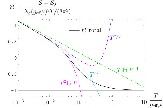
Figure 4.3: The first few orders of the low-temperature series for the entropy density in comparison with the full HDL-resummed result (from [113]).

In Eq. (4.165) we have neglected terms like $g_{\rm eff}^{2}b^{6}\equiv(T/\mu)^{2}$ in $P/(g_{\rm eff}^{4}\mu^{4})$, therefore we have to assume $T\ll\mu$. This is however a weaker condition for the temperature than the condition $T\ll g_{\rm eff}\mu$ which we had in the previous subsections. The weaker condition is sufficient now, because we do not perform an expansion in $b$ in this subsection. Adding the soft contribution from Eq. (4.165), the hard contribution from Eqs. (4.110) and (4.113), and the non-$n_{b}$ contribution from Eq. (4.131), we arrive at the following result for the entropy density [113],

$$\!\!\!\!\!\!\!\!\!\!{1\over N_{g}}\left(\mathcal{S}-\mathcal{S}^{0}\right)=-{g_{\rm eff}^{2}\mu^{2}T\over 24\pi^{2}}-{1\over 2\pi^{3}}\int_{0}^{\infty}dq_{0}{\partial n_{b}(q_{0})\over\partial T}\int_{0}^{2\mu}dq\,q^{2}$$

$$\times\left[2\mathrm{Im}\log\left(q^{2}-q_{0}^{2}+\tilde{\Pi}_{T}\right)+\mathrm{Im}\log\left({q^{2}-q_{0}^{2}+\tilde{\Pi}_{L}\over q^{2}-q_{0}^{2}}\right)\right]+\mathcal{O}(g_{\rm eff}^{4}\mu^{2}T),$$

(4.166)

where $\mathcal{S}^{0}$ is the ideal-gas entropy density. The right hand side of Eq. (4.166) is essentially given by one universal function of the dimensionless variable $T/(g_{\rm eff}\mu)$, which we define through [113]

$${8\pi^{2}\over N_{g}g_{\rm eff}^{2}\mu^{2}T}\left(\mathcal{S}-\mathcal{S}^{0}\right)=:\mathfrak{S}\left({T\over g_{\rm eff}\mu}\right)+\mathcal{O}(g_{\rm eff}^{2}).$$ (4.167)

and which we have normalized such that the ordinary perturbative two-loop result [114, 115] for the low-temperature entropy density corresponds to $\mathfrak{S}=-1$. The function $\mathfrak{S}$ can be evaluated numerically. Fig 4.3 shows a comparison of the first few orders of the low-temperature series with the full HDL result taken from [113]. Further numerical results, in particular a comparison with non-perturbative large-$N_{f}$ results, can be found in [100, 113].

4.6 Some remarks on neutrino emission from ungapped quark matter

A young neutron star loses energy mainly via neutrino emission from the bulk [33, 57]. One generally distinguishes fast processes, which lead to neutrino emissivities proportional to $T^{6}$, and slow processes which lead to neutrino emissivities proportional to $T^{8}$, see e.g. [33] and references therein. The dominant process for neutrino emission from ungapped quark matter is the quark analogon of the direct Urca process [57, 116, 117],

$$d \to u+e^{-}+\bar{\nu}_{e},$$ (4.168)

$$u+e^{-} \to d+\nu_{e}.$$ (4.169)

The cooling behavior is governed by the cooling equation

$$\mathcal{C}_{v}(T){\partial T\over\partial t}=-\epsilon(T),$$ (4.170)

where $\epsilon(T)$ is the neutrino emissivity, which is given by [57, 116, 117]

$$\epsilon(T)=3\sum_{\sigma_{u},\sigma_{d},\sigma_{e}}\int{d^{3}p_{d}\over(2\pi)^{3}}{1\over 2E_{d}}\int{d^{3}p_{u}\over(2\pi)^{3}}{1\over 2E_{u}}\int{d^{3}p_{e}\over(2\pi)^{3}}{1\over 2E_{e}}\int{d^{3}p_{\nu}\over(2\pi)^{3}}{1\over 2E_{\nu}}E_{\nu}$$

$$\qquad\times\bigg{[}|M_{\beta}|^{2}(2\pi)^{4}\delta^{4}(P_{d}-P_{u}-P_{e}-P_{\nu})$$

$$\qquad\qquad\times n_{f}(E_{d}-\mu_{d})[1-n_{f}(E_{u}-\mu_{u})][1-n_{f}(E_{e}-\mu_{e})]$$

$$\qquad\quad+|M_{ec}|^{2}(2\pi)^{4}\delta^{4}(p_{u}+p_{e}-p_{d}-p_{\nu})$$

$$\qquad\qquad\times n_{f}(E_{u}-\mu_{u})n_{f}(E_{e}-\mu_{e})[1-n_{f}(E_{d}-\mu_{d})]\bigg{]},$$ (4.171)

where $\sigma_{i}$ are the fermion helicities, $E_{i}$ are the energies of the fermionic quasiparticles as determined from the poles of the propagators (neglecting the imaginary parts of the self energies), $M_{\beta}$ is the matrix element for the reaction (4.168), and $M_{ec}$ is the matrix element for the reaction (4.169).

In [57] it is shown that the emissivity through leading logarithmic order can be written as

$$\!\!\!\!\!\!\!\!\!\!\!\!\!\!\!\!\!\!\!\!\!\!\!\!\!\!\!\epsilon(T)={2g^{2}G_{F}^{2}\cos^{2}\theta_{c}\over\pi^{7}}\mu_{e}\mu_{q}^{2}T^{6}\int_{-\infty}^{\infty}dx_{d}\int_{-\infty}^{\infty}dx_{u}\int_{0}^{\infty}dx_{\nu}\,x_{\nu}^{3}$$

$$\!\!\!\!\!\!\!\!\!\!\!\!\!\!\!\!\!\!\times n_{f}(Tx_{d})n_{f}(-Tx_{u})n_{f}(T(x_{u}-x_{d}+x_{\nu}))\,v_{g}^{-1}(E_{d})\,v_{g}^{-1}(E_{u})\Big{|}_{E_{i}\to\mu_{i}+Tx_{i}},$$ (4.172)

where $G_{F}$ is the Fermi coupling, $\theta_{c}$ is the Cabibbo angle, and $\mu_{q}\simeq\mu_{u}\simeq\mu_{d}$. The inverse group velocity $v_{g}^{-1}$, as defined in Eq. (3.103), contains non-Fermi-liquid contributions, which we have discussed in chapter 3. As shown in [57] the non-Fermi-liquid corrections to the specific heat and the emissivity lead to a (modest) reduction of the temperature at late times.

If one wants to go beyond the leading logarithmic accuracy of Ref. [57], at least the following ingredients will be required. First, there will be corrections to the emissivity from gluonic corrections to the weak interaction vertex [57]. It might also be necessary to generalize the formula (4.171) for the emissivity in a way that takes into account the finite lifetime of the fermionic quasiparticles, since the imaginary part of the quark self energy is of the same order as the term which fixes the scale under the logarithm in the real part.

As a first step towards a more complete computation of the emissivity, let us take the scale under the leading logarithm of the group velocity as given by Eqs. (3.67) and (3.68), and simply insert the resulting expression for the group velocity into Eq. (4.172). Using the integral

$$\int_{-\infty}^{\infty}dx_{1}\int_{-\infty}^{\infty}dx_{1}\int_{0}^{\infty}dx_{3}\,n_{f}(Tx_{1})n_{f}(-Tx_{2})n_{f}(T(x_{2}-x_{1}+x_{3}))$$

$$\qquad\times{\partial\over\partial\alpha}\left(\mathrm{Li}_{\alpha}(-e^{-x_{1}})+\mathrm{Li}_{\alpha}(-e^{x_{1}})\right)\Big{|}_{\alpha=0}=-105.303\ldots$$ (4.173)

we would then find

$$\epsilon(T)\simeq{457\over 2520\pi}g^{2}G_{F}^{2}\cos^{2}\theta_{c}\,\mu_{q}^{2}\mu_{e}T^{6}\left(1+{2g^{2}\over 9\pi^{2}}\log\left({4.295m\over T}\right)\right).$$ (4.174)

While the constant under the logarithm will certainly be modified in a more complete computation as discussed above, it is already interesting to note that this constant is about an order of magnitude larger than the corresponding constant in the specific heat, which we find to be approximately equal to $0.282$ from Eq. (4.163).

Chapter 5 Color superconductivity

5.1 Basics of superconductivity

Since its experimental discovery in 1911, superconductivity has been extensively studied both in experimental and theoretical condensed matter physics. The first microscopic theory of superconductivity was developed by Bardeen, Cooper and Schrieffer (BCS) in 1957 [118], see e.g. [106, 119, 120] for pedagogical reviews. The key observation is that the electron-phonon interaction induces an effective electron-electron interaction which is attractive. This leads to the formation of Cooper pairs. The ground state, which is different from the ground state of a normal Fermi liquid, is then given by

$$|\Psi\rangle=\prod_{\bf k}\left(u_{\bf k}+v_{\bf k}c_{{\bf k}\uparrow}^{\dagger}c_{-{\bf k}\downarrow}^{\dagger}\right)|0\rangle,$$ (5.1)

where $c_{{\bf k}\uparrow}^{\dagger}$ and $c_{{\bf k}\downarrow}^{\dagger}$ are creation operators for electrons with spin up and spin down, respectively. The coefficients $u_{\bf k}$ and $v_{\bf k}$ are determined by minimization of the free energy. The state (5.1) can be characterized by a non-vanishing “di-electron” condensate,

$$\langle\psi\psi\rangle\neq 0,$$ (5.2)

which leads to a gap in the fermionic quasiparticle spectrum. A condensate like (5.2) breaks spontaneously the $U(1)$ invariance of electrodynamics. Therefore the photon will acquire a mass via the Higgs mechanism. This leads to the Meissner effect, namely the screening of magnetic fields inside a superconductor.

5.2 Basics of color superconductivity

Let us begin with an ensemble of free quarks. At finite density the ground state of this system is simply given by a Fermi sphere. Now let us turn on interactions. At asymptotic densities at first sight a purely perturbative treatment might seem appropriate because the interactions are “weak” due to asymptotic freedom. However, it is important to note that single gluon exchange is attractive in the color antitriplet channel. This has dramatic consequences, since an arbitrarily weak attractive interaction leads to the Cooper instability of the Fermi surface, and the ground state will contain diquark condensates,

$$\Phi^{ij,fg,\alpha\beta}\sim\langle\psi_{c}^{i,f,\alpha}({\bf p})\bar{\psi}^{i,g,\beta}(-{\bf p})\rangle\neq 0,$$ (5.4)

where $i$, $j$ are fundamental color indices, $f$, $g$ are flavor indices, $\alpha$, $\beta$ are spinor indices, and $\psi_{c}$ denotes the charge conjugated spinor, $\psi_{c}=C\bar{\psi}^{T}$. By virtue of its similarity to superconductivity in ordinary condensed matter physics, this phenomenon was termed color superconductivity.

In the usual notation for the irreducible SU(3) representations one has

$${\bf 3}\otimes{\bf 3}={\bf 6}\oplus{\bf\bar{3}}.$$ (5.5)

Therefore one cannot construct a color singlet from the expectation value (5.4). This means that global color symmetry is spontaneously broken by the diquark condensate.

Quarks have color, flavor and spin as internal degrees of freedom. Therefore quite many different color superconducting phases could be possible, depending on the color, flavor and spin structure of the expectation value (5.4). At very high densities the phase with the lowest free energy is the so-called color flavor locked (CFL) phase [123, 124, 125, 126], where up, down and strange quarks contribute to the pairing on an equal footing,

$$\Phi_{\mathrm{CFL}}\propto\varepsilon^{ijA}\varepsilon^{fgA}=\delta^{if}\delta^{jg}-\delta^{ig}\delta^{jf}.$$ (5.6)

The symmetry breaking pattern of the CFL phase is (neglecting electromagnetism and quark masses for the moment)

$$SU(3)_{c}\times SU(3)_{L}\times SU(3)_{R}\times U(1)_{B}\to SU(3)_{c+L+R}\times{\mathbbm{Z}}_{2}.$$ (5.7)

Here $SU(3)_{c}$ corresponds to global color symmetry, $SU(3)_{R,L}$ correspond to right and left handed flavor symmetry, and $U(1)_{B}$ corresponds to baryon number conservation. These symmetries are broken down to the diagonal subgroup $SU(3)_{c+L+R}$ times a ${\mathbbm{Z}}_{2}$ group that corresponds to $\psi\to-\psi$. In the CFL phase all eight gluons acquire a mass through the Higgs mechanism [127, 128, 129]. The electromagnetic $U(1)$ symmetry is also broken, but there remains an unbroken $\tilde{U}(1)$ [123, 130], whose generator is given by $\tilde{Q}_{\mathrm{CFL}}=Q+{2\over\sqrt{3}}T_{8}$, with $Q=\mathrm{diag}(-{1\over 3},-{1\over 3},{2\over 3})$ in flavor space, and $T_{8}={1\over 2\sqrt{3}}\mathrm{diag}(1,1,-2)$ in color space.

As in every field theoretical model with spontaneous symmetry breaking, Nambu-Goldstone bosons appear in the CFL phase [127, 131, 132, 133, 134, 135]. Because of the symmetry breaking pattern (5.7) there are 17 broken generators, which would lead to 17 Nambu-Goldstone bosons. Eight of these, corresponding to the breaking of $SU(3)_{c}$, are “eaten” by the gluons. The “surviving” Nambu-Goldstone bosons are an octet corresponding to flavor symmetry breaking and a singlet corresponding to baryon number breaking. While this singlet boson is strictly massless, the octet bosons become massive if finite quark masses are taken into account. Furthermore there is a light singlet from $U(1)_{A}$ breaking.

At lower densities, the strange quark will eventually decouple, which should lead to a two-flavor color superconducting (2SC) phase [38, 39, 40], where only up and down quarks participate in the pairing,

$$\Phi_{\mathrm{2SC}}\propto\varepsilon^{ij3}\varepsilon^{fg3}.$$ (5.8)

In the 2SC phase the global color symmetry group $SU(3)_{c}$ is broken down to $SU(2)_{c}$, but flavor symmetry remains unbroken. Therefore there are five would-be Nambu-Goldstone bosons [136, 137, 138], which are “eaten” by the gluons. The gluons with adjoint colors $1$-$3$ are massless, while the gluons with adjoint colors $4$-$8$ acquire a mass through the Higgs mechanism [139, 140]. As in the CFL phase the electromagnetic $U(1)$ symmetry is broken, but again an unbroken $\tilde{U}(1)$ survives [136, 141], whose generator is now given by $\tilde{Q}_{\mathrm{2SC}}={1\over 3\sqrt{2}}({\bf 1}-2\sqrt{3}T_{8})$.

In Ref. [142] it was argued that the 2SC phase will be disfavored if one takes into account the constraints from color and electric charge neutrality at finite strange quark mass $m_{s}$. To date a completely reliable description of the phase structure of QCD at densities below the CFL regime is still lacking. In the following we will list some of the phases that have been proposed in the literature.

Computing the meson masses from the low energy effective Lagrangian in the CFL phase, one finds that the masses of the $K^{+}$ and $K^{0}$ become imaginary if $m_{s}$ exceeds a certain value. This indicates the formation of a kaon condensate [44, 143, 144, 145].

The charge neutrality condition and the finite strange quark mass lead to a mismatch of the Fermi momenta of the different quark flavors. This might give rise to so-called gapless superconducting phases (g2SC [47, 48, 146, 147] and gCFL [148, 149, 150, 151]), where the fermionic quasiparticle dispersion laws are modified, some of them corresponding to gapless excitations. In Refs. [152, 153, 154] however, it was found that the Meissner masses are imaginary in these phases. This would indicate that the gapless phases are unstable, if no mechanism can be found which makes the Meissner masses real quantities.

So far we have assumed only spin zero diquark condensates. The gaps resulting from spin one condensates are much smaller than in the spin zero case. Nevertheless spin one condensates might play a certain role at intermediate densities, since they may be formed from quarks of the same flavor, see Refs. [38, 155, 156, 157, 158, 159].

The mismatch of the Fermi momenta might also induce a so-called LOFF (Larkin-Ovchinnikov-Fulde-Ferrell) pairing [56, 160, 161, 162, 163]. The LOFF state is characterized by Cooper pairs with non-zero total momentum, and therefore translational and rotational symmetry are spontaneously broken. This leads to crystalline structures that might have relevant consequences for astrophysics [41].

5.3 The color superconductivity gap equation

The gap equation for a color superconducting phase can be derived from the Schwinger-Dyson equation for the quark two-point function, allowing for a non-vanishing expectation value (5.4). At this point it is convenient to introduce a Nambu-Gor’kov basis for the quark spinors, which is given by $\Psi=(\psi,\psi_{c})^{T}$, $\bar{\Psi}=(\bar{\psi},\bar{\psi}_{c})$. The inverse quark propagator in this basis is given by [38, 164, 165]

$$S^{-1}=\left(\begin{array}[]{cc}\not{Q}+\mu\gamma_{0}+\Sigma&\Phi^{-}\\ \Phi^{+}&\not{Q}-\mu\gamma_{0}+\bar{\Sigma}\end{array}\right),$$ (5.9)

where $\Phi^{\pm}$ are the gap functions, related by $\Phi^{-}(Q)=\gamma_{0}[\Phi^{+}(Q)]^{\dagger}\gamma_{0}$, and $\Sigma(Q)$ is the quark self energy, with $\bar{\Sigma}(Q)=C[\Sigma(-Q)]^{T}C^{-1}$. Flavor and fundamental color indices are suppressed in Eq. (5.9).

In order to solve the Schwinger-Dyson equation a suitable approximation scheme has to be chosen. To date only the exponent and the leading contribution to the prefactor of the gap [see Eq. (5.13) below] have been determined consistently, where the following set of approximations turned out to suffice:

• replace the full quark-gluon vertex with its tree level counterpart (at least in Coulomb gauge) [166],

• replace the full gluon propagator with its HDL approximation [167],

• replace the quark self energy with the leading logarithmic result of the normal phase (see Eq. (3.67)) [164].

A rather lengthy calculation [45, 156, 164] then yields the following gap equation for the 2SC phase (neglecting the gauge dependent part)

$$\phi^{+}(\epsilon_{\bf k},k)={g^{2}\over 18\pi^{2}}\int_{0}^{\delta}d(q-\mu)Z(\epsilon_{\bf q}){\phi^{+}(\epsilon_{\bf q},q)\over\epsilon_{\bf q}}\tanh\left({\epsilon_{\bf q}\over 2T}\right){1\over 2}\log\left({b^{2}\mu^{2}\over|\epsilon_{\bf q}^{2}-\epsilon_{\bf k}^{2}|}\right),$$ (5.10)

where $\epsilon_{\bf k}=\sqrt{(k-\mu)^{2}+|\phi^{+}|^{2}}$, $\delta\sim\mathcal{O}(g\mu)$ is a cutoff, $b=256\pi^{4}(2/(N_{f}g^{2}))^{5/2}$, and

$$Z(E-\mu)=\left[1-{\partial\mathrm{Re}\Sigma_{+}\over\partial(E-\mu)}\right]^{-1}$$ (5.11)

is usually called “wave function renormalization factor” in this context (in the previous chapters we referred to this quantity as group velocity). With the definition

$$x={g\over 3\sqrt{2}\pi}\log\left({2b\mu\over k-\mu+\epsilon_{\bf k}}\right)$$ (5.12)

the solution of the gap equation at zero temperature can be written as [86, 156, 164, 168, 169, 170, 171]

$$\phi^{+}=2bb_{0}^{\prime}\mu\exp\left(-{3\pi^{2}\over\sqrt{2}g}\right)F(x),$$ (5.13)

where $b_{0}^{\prime}=\exp[-(\pi^{2}+4)/8]$. $F(x)$ is quite a complicated function, which is given explicitly in [164]. At the Fermi surface $F(x)$ is equal to $1+\mathcal{O}(g^{2})$, and away from the Fermi surface it decreases rapidly.

The parametric dependence of the gap on the coupling constant as shown in Eq. (5.13) was first derived by Son [168] using renormalization group techniques. It is different from the BCS result $\phi^{+}\sim\exp(-1/g^{2})$, which is a consequence of the fact that quasistatic chromomagnetic interactions are only dynamically screened.

The result for the gap can also be derived within the framework of high density effective theory (HDET), in which the only relevant fermionic degrees of freedom are those in the vicinity of the Fermi surface [43, 172, 173, 174, 175].

In the literature also the possible gauge dependence of the prefactor of the gap, which would indicate an inconsistent approximation scheme, has been discussed. In [176] the gap equation was solved numerically in a general covariant gauge, with the result that large gauge dependences occur for $g>g_{c}\sim 0.8$. In Ref. [177], however, it was argued that in a covariant gauge one has to include the quark gluon vertex correction in order to obtain a gauge independent result. In [178] it was shown that the prefactor of the gap is gauge independent in a general Coulomb gauge, if the gap is evaluated on the quasiparticle mass shell. In the next section we will give a general proof that the fermionic quasiparticle dispersion laws in a color superconductor are gauge independent [179].

5.4 Gauge independence of fermionic dispersion laws

The inverse quark propagator in the Nambu-Gor’kov basis, as shown in Eq. (5.9), is the momentum space version of the second derivative of the effective action,

$${\delta^{2}\Gamma\over\delta\bar{\Psi}(x)\delta\Psi(y)}\Big{|}_{\psi=\bar{\psi}=A_{i}^{a}=0,A_{0}^{a}=\bar{A}_{0}^{a}},$$ (5.14)

where $\Psi=(\psi,\psi_{c})^{T}$, $\bar{\Psi}=(\bar{\psi},\bar{\psi}_{c})$, and $\bar{A}_{0}^{a}$ is the expectation value of $A_{0}^{a}$, which is in general non-vanishing (see Sec. 5.6).

It should be noted that the doubling of fermionic fields in terms of $\Psi$ and $\bar{\Psi}$ is just a notational convenience here; the effective action itself should be viewed as depending only on either $(\psi,\bar{\psi})$ or the set $\Psi=(\psi,\psi_{c})^{T}$.

The gauge dependence identity for the effective action [Eq. (2.12)] can be written as

$$\!\!\!\!\!\!\!\!\!\!\!\!\!\!\!\!\delta\Gamma=\int d^{4}x\left({\delta\Gamma\over\delta\psi(x)}\delta X_{(\psi)}(x)-\delta X_{(\bar{\psi})}(x){\delta\Gamma\over\delta\bar{\psi}(x)}+{\delta\Gamma\over\delta A^{a\mu}(x)}\delta X_{(A)}^{a\mu}(x)\right)$$

$$\!\!\!\!\!\!\!\equiv\int d^{4}x\left({\delta\Gamma\over\delta\psi(x)}\delta X_{(\psi)}(x)+{\delta\Gamma\over\delta\psi_{c}(x)}\delta X_{(\psi_{c})}(x)+{\delta\Gamma\over\delta A^{a\mu}(x)}\delta X_{(A)}^{a\mu}(x)\right),\quad$$ (5.15)

Eq. (5.15) can be cast in a more compact form using the DeWitt notation, but now only for the fermions,

$$\delta\Gamma=\Gamma_{,i}\delta X^{i}+\int d^{4}x{\delta\Gamma\over\delta A^{a\mu}(x)}\delta X_{(A)}^{a\mu}(x),$$ (5.16)

where $i=(\psi(x),\psi_{c}(x))^{T}$, $\bar{i}=(\bar{\psi}(x),\bar{\psi}_{c}(x))$, and the comma denotes functional derivation. Taking the second derivative of (5.16), setting $\psi=\bar{\psi}=A^{a}_{i}=0$, $A^{a}_{0}=\bar{A}^{a}_{0}$, and using the fact that

$${\delta\Gamma\over\delta A^{a}_{0}}\Big{|}_{\psi=\bar{\psi}=A^{a}_{i}=0,A^{a}_{0}=\bar{A}^{a}_{0}}=0,$$ (5.17)

we obtain a gauge dependence identity for the inverse propagator (5.14),

$$\delta\Gamma_{i\bar{j}}=-\Gamma_{k\bar{j}}\delta X^{k}_{\,,i}+\Gamma_{ki}\delta X^{k}_{\,,\bar{j}}+\int d^{4}x{\delta\Gamma_{i\bar{j}}\over\delta A^{a0}(x)}\delta X_{(A)}^{a0}(x).$$ (5.18)

Up to this point, our functional relations are completely general and apply also to the case of inhomogeneous color superconducting phases. We do not attempt to cover the complications this case may add to the question of gauge independence, but continue by assuming translational invariance. This allows us to introduce $\delta\bar{A}^{a0}:=-\delta X_{(A)}^{a0}(x=0)$ and to write (5.18) as

$$\delta\Gamma_{i\bar{j}}=-\Gamma_{k\bar{j}}\delta X^{k}_{\,,i}-\delta X^{\bar{k}}_{\,,\bar{j}}\Gamma_{i\bar{k}}-{\partial\Gamma_{i\bar{j}}\over\partial\bar{A}^{a0}}\delta\bar{A}^{a0}.$$ (5.19)

Furthermore, we can transform Eq. (5.19) into momentum space,

$$\delta\Gamma_{i\bar{j}}(Q)+\delta\bar{A}^{a0}{\partial\Gamma_{i\bar{j}}(Q)\over\partial\bar{A}^{a0}}=-\Gamma_{k\bar{j}}(Q)\delta X^{k}_{\,,i}(Q)-\delta X^{\bar{k}}_{\,,\bar{j}}(Q)\Gamma_{i\bar{k}}(Q),$$ (5.20)

where the indices $i$ and $\bar{i}$ from now on comprise only color, flavor, Dirac and Nambu-Gor’kov indices. Using Eq. (C.1) we obtain

$$\delta\det(\Gamma_{i\bar{j}})+\delta\bar{A}^{a0}{\partial\over\partial\bar{A}^{a0}}\det(\Gamma_{i\bar{j}})\equiv\delta_{\rm tot}\det(\Gamma_{i\bar{j}})=-\det(\Gamma_{i\bar{j}})[\delta X^{k}_{\,,k}+\delta X^{\bar{k}}_{\,,\bar{k}}].$$ (5.21)

The left hand side of this identity is the total variation [62, 63] of the determinant of the inverse quark propagator, with the first term corresponding to the explicit variation of the gauge fixing function, and the second term coming from the gauge dependence of $\bar{A}_{0}^{a}$.

Since the determinant is equal to the product of the eigenvalues, Eq. (5.21) implies that the location of the singularities of the quark propagator is gauge independent, provided that the singularities of $\delta X^{k}_{\,,k}$ do not coincide with those of the quark propagator. The singularity structure of $\delta X$ may be discussed in a similar way as in the case of the Higgs model, see Sec. 2.3.3. The quantity $\delta X$ is 1PI up to a full ghost propagator, and up to gluon tadpole insertions (see Ref. [60] for the explicit diagrammatic structure) . As in [60, 64] one may argue that the singularities of the ghost propagator are not correlated to the singularities of the quark propagator. Gauge independence of the zeros of the inverse fermion propagator then follows provided that also the 1PI parts of $\delta X$ have no singularities coinciding with the singularities of the fermion propagator. An important caveat in fact comes from massless poles in the unphysical degrees of freedom of the gauge boson propagator, which are typical in covariant gauges and which can give rise to spurious mass shell singularities as encountered in the case of hot QCD in [73]. But, as was pointed out in [74], these apparent gauge dependences are avoided if the quasiparticle mass-shell is approached with a general infrared cut-off such as finite volume, and this cut-off lifted only in the end, i.e., after the mass-shell limit has been taken.

The determinant which appears in (5.21) is taken with respect to color, flavor, Dirac and Nambu-Gor’kov indices. The determinant in Nambu-Gor’kov space may be evaluated explicitly using Eq. (C.2). From Eq. (5.9) we obtain in this way

$$\det(\Gamma_{i\bar{j}}) = \det\big{[}(\not{Q}-\mu\gamma_{0}+\bar{\Sigma})(\not{Q}+\mu\gamma_{0}+\Sigma)$$ (5.22)

$$\qquad-(\not{Q}-\mu\gamma_{0}+\bar{\Sigma})\Phi^{-}(\not{Q}-\mu\gamma_{0}+\bar{\Sigma})^{-1}\Phi^{+}\big{]}.\qquad$$

The inverse of the matrix of which the determinant is taken here appears, of course, in the ordinary quark propagator, which is obtained by inverting (5.9),

$$\!\!\!\!\!\!\!\!\!\mathcal{G}^{+}(Q)=\big{[}(\not{Q}-\mu\gamma_{0}+\bar{\Sigma})(\not{Q}+\mu\gamma_{0}+\Sigma)$$

$$\qquad\quad-(\not{Q}-\mu\gamma_{0}+\bar{\Sigma})\Phi^{-}(\not{Q}-\mu\gamma_{0}+\bar{\Sigma})^{-1}\Phi^{+}\big{]}^{-1}(\not{Q}-\mu\gamma_{0}+\bar{\Sigma}).\qquad$$ (5.23)

At leading order, when the quark self energy $\Sigma$ can be neglected, (5.22) can be approximated by

$$\det(\Gamma_{i\bar{j}})\simeq\det\left[(\not{Q}-\mu\gamma_{0})(\not{Q}+\mu\gamma_{0})-(\not{Q}-\mu\gamma_{0})\Phi^{-}(\not{Q}-\mu\gamma_{0})^{-1}\Phi^{+}\right].$$ (5.24)

This expression can be rewritten as

$$\det(\Gamma_{i\bar{j}}) \simeq \det\Big{[}\left(q_{0}^{2}-(q-\mu)^{2}-(\phi_{r+}^{+})^{\dagger}\phi_{r+}^{+}\right)\mathcal{P}_{r+}^{+}$$ (5.25)

$$\quad\ +\left(q_{0}^{2}-(q-\mu)^{2}-(\phi_{l-}^{+})^{\dagger}\phi_{l-}^{+}\right)\mathcal{P}_{l-}^{+}$$

$$\quad\ +\left(q_{0}^{2}-(q+\mu)^{2}-(\phi_{r-}^{-})^{\dagger}\phi_{r-}^{-}\right)\mathcal{P}_{r-}^{-}$$

$$\quad\ +\left(q_{0}^{2}-(q+\mu)^{2}-(\phi_{l+}^{-})^{\dagger}\phi_{l+}^{-}\right)\mathcal{P}_{l+}^{-}\Big{]},$$

where the projection operators introduced in [180] are given by

$$\mathcal{P}_{r,l\pm}^{\pm}=\mathcal{P}_{r,l}\mathcal{P}_{\pm}({\bf q})\Lambda^{\pm}({\bf q}),$$ (5.26)

where $\mathcal{P}_{r,l}={1\over 2}(1\pm\gamma_{5})$ is the chirality projector, $\mathcal{P}_{\pm}({\bf q})={1\over 2}(1\pm\gamma_{5}\gamma_{0}\gamma^{i}\hat{q}^{i})$ is the helicity projector, and $\Lambda^{\pm}({\bf q})$ is the energy projector given in Eq. (3.42). (Note that $\mathcal{P}^{+}_{r-}=\mathcal{P}^{+}_{l+}=\mathcal{P}^{-}_{r+}=\mathcal{P}^{-}_{l-}=0$ in the massless limit which we are considering here [180].) If we assume for simplicity that $\phi^{\dagger}\phi$ is diagonal with respect to color and flavor indices, the determinant in Eq. (5.25) can be readily evaluated,

$$\det(\Gamma_{i\bar{j}}) \simeq \prod_{f}\left(q_{0}^{2}-(q-\mu)^{2}-|\phi_{r+}^{+(f)}|^{2}\right)\left(q_{0}^{2}-(q-\mu)^{2}-|\phi_{l-}^{+(f)}|^{2}\right)$$ (5.27)

$$\!\!\times\left(q_{0}^{2}-(q+\mu)^{2}-|\phi_{r-}^{-(f)}|^{2}\right)\left(q_{0}^{2}-(q+\mu)^{2}-|\phi_{l+}^{-(f)}|^{2}\right),\qquad$$

giving the well known branches of the quasiparticle excitation spectrum for each value of the color-flavor index $f$ [180].

At leading order, when the quark self energy can be neglected, Eqs. (5.21) and (5.22) imply that the gap function is gauge independent on the quasiparticle mass shell. It should be noted, however, that at higher orders only dispersion relations obtained from (5.22), which also include the quark self energy $\Sigma$, can be expected to be gauge independent.

We note furthermore that for $\Phi^{\pm}\to 0$ the determinant (5.22) becomes

$$\det\left[(\not{Q}+\mu\gamma_{0}+\Sigma)(\not{Q}-\mu\gamma_{0}+\bar{\Sigma})\right]=\det(\mathcal{G}^{+}_{0}(Q)^{-1})\times\det(\mathcal{G}^{+}_{0}(-Q)^{-1}),$$ (5.28)

where $\mathcal{G}^{+}_{0}(Q)=[\not{Q}+\mu\gamma_{0}+\Sigma]^{-1}$. Therefore, in this case the gauge independence proof, of course, boils down to the gauge independence proof for the singularities of the quark propagator without diquark condensates.

5.5 Computation of $\delta X$

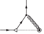
Figure 5.1: Feynman diagram for $\delta X_{(1)}$ (see Eq. (5.29)).

The aim of this subsection is the evaluation of $\delta X^{k}_{\,,k}$ for the 2SC phase in covariant gauge. This is interesting because the existing calculations in the literature give gauge dependent results for the gap in this gauge.

We will focus on possible singularities of $\delta X^{k}_{\,,k}$, since they might invalidate the above proof of gauge independence. At one-loop level $\delta X^{k}_{\,,k}$ contains terms like

$$\delta X_{(1)}(K):=g^{2}\int{d^{4}Q\over i(2\pi)^{4}}\mathrm{Tr}_{D,c,f}\bigg{[}T_{a}{1\over P^{2}}{1\over\sqrt{2\xi}}P^{\mu}D_{\mu\nu}(P)\mathcal{G}^{+}(Q)\gamma^{\nu}T_{a}$$

$$\qquad\qquad\qquad+T_{a}^{T}{1\over P^{2}}{1\over\sqrt{2\xi}}P^{\mu}D_{\mu\nu}(P)\mathcal{G}^{-}(Q)\gamma^{\nu}T_{a}^{T}\bigg{]},$$ (5.29)

where $P=K-Q$, $D_{\mu\nu}$ is the gluon propagator, $\mathcal{G}^{\pm}$ is the quark propagator (see below), and we have used

$$D^{i}_{\alpha} \rightarrow -igT_{a}\psi,\ igT_{a}^{T}\psi_{c}$$ (5.30)

$$\mathcal{G}^{\alpha}_{\ \beta} \rightarrow {1\over P^{2}}\delta^{ab},$$ (5.31)

$$\delta F^{\alpha}\propto F^{\alpha} \rightarrow {1\over\sqrt{2\xi}}P^{\mu}A_{\mu}^{a}.$$ (5.32)

Eq. (5.29) corresponds to the diagram in Fig. 5.1, where the vertex with a circle denotes $\delta F^{\alpha}$ and the small triangle denotes $D_{\alpha}^{i}$.

In the 2SC phase the gap matrix is given by [39, 156]

$$[\Phi^{+}]_{ij}^{fg}=\varepsilon^{fg}\varepsilon_{ij3}(\phi^{+}(\mathcal{P}^{+}_{r+}-\mathcal{P}^{+}_{l-})+\phi^{-}(\mathcal{P}^{-}_{r-}-\mathcal{P}^{-}_{l+})),$$ (5.33)

where $f$, $g$ are flavor indices and $i$, $j$ are fundamental color indices. The $\mathcal{P}$’s are the projection operators defined in Eq. (5.26). We have assumed for simplicity that the right-handed and the left-handed gap functions are equal up to a sign [156]. For the quark propagator $\mathcal{G}^{\pm}(Q)$ one finds then [139]

$$[\mathcal{G}^{\pm}]_{ij}^{fg}=\delta^{fg}\left[(\delta_{ij}-\delta_{i3}\delta_{j3})G^{\pm}+\delta_{i3}\delta_{j3}G^{\pm}_{0}\right],$$ (5.34)

with [139]

$$G^{\pm}(Q) = \sum_{e=\pm}{q_{0}\mp(\mu-eq)\over q_{0}^{2}-(\mu-eq)^{2}-|\phi^{e}|^{2}}\Lambda^{\pm e}({\bf q})\gamma_{0},$$ (5.35)

$$G^{\pm}_{0}(Q) = \sum_{e=\pm}{q_{0}\mp(\mu-eq)\over q_{0}^{2}-(\mu-eq)^{2}}\Lambda^{\pm e}({\bf q})\gamma_{0},$$ (5.36)

where $\Lambda^{\pm}$ are the energy projectors given in Eq. (3.42). We shall consider only the part of $\delta X_{(1)}$ which contains the propagator $G^{\pm}$, because it is this part which depends on the condensate. We will call this part $\delta X_{(11)}$. In the HDL approximation the gluon propagator obeys the following Ward identity,

$$P^{\mu}D_{\mu\nu}(P)=\xi{P_{\nu}\over P^{2}}.$$ (5.37)

Thus we obtain after taking the color trace, neglecting the antiparticle propagator and the imaginary part of the gap function [156], and dropping an irrelevant prefactor

$$\!\!\!\!\!\!\!\!\delta X_{(11)}(K)=2g^{2}\sqrt{\xi}\int{d^{4}Q\over i(2\pi)^{4}}{1\over(P^{2})^{2}}{q_{0}\over q_{0}^{2}-(\mu-q)^{2}-(\phi^{+})^{2}}\mathrm{Tr}_{D}[\Lambda^{+}_{\bf q}\gamma_{0}\gamma_{\nu}]P^{\nu}$$

$$\!\!\!\!=4g^{2}\sqrt{\xi}\int{d^{4}Q\over i(2\pi)^{4}}{1\over(p_{0}^{2}-p^{2})^{2}}{q_{0}(p_{0}-{\bf p}\cdot{\bf\hat{q}})\over q_{0}^{2}-(\mu-q)^{2}-(\phi^{+})^{2}}=$$

$$\!\!\!\!=4g^{2}\sqrt{\xi}\int{d^{4}Q\over i(2\pi)^{4}}{-iq_{4}(i(k_{4}-q_{4})-kt+q)\over[(k_{4}-q_{4})^{2}+(k^{2}+q^{2}-2kqt)]^{2}(q_{4}^{2}+(\mu-q)^{2}+(\phi^{+})^{2})},\quad$$

where $t=\cos\theta$ and $q_{4}=-iq_{0}$. The integral is dominated by $\theta\simeq 0$, therefore we may set $t=1$ in the numerator. We set $k=\mu$ and define $\zeta=q-\mu$. After carrying out the $q_{4}$-integration (assuming that $\phi^{+}$ is almost independent of $q_{4}$) we perform the analytical continuation $k_{4}\to ik_{0}$ and take the on-shell limit, $k_{0}\to\phi^{+}$. Then the $\zeta$-integral (with UV cutoff $\pm\mu$) gives terms proportional to $\log(k_{0}^{2}-(\phi^{+})^{2})$. Thus there may be indeed a mass shell singularity in $\delta X$, at least within our approximations. It is however only a logarithmic singularity, which is harmless because on the right hand side of the gauge dependence identity we have expressions like

$$(k_{0}^{2}-(\phi^{+})^{2})\left(\log(k_{0}^{2}-(\phi^{+})^{2})+\mathrm{finite}\right),$$ (5.39)

which vanish for $k_{0}\rightarrow\phi$. We conclude that no IR cutoff should be necessary to assure gauge independence of the dispersion laws (at zero temperature).

An explicit calculation shows indeed that a simple IR cutoff for the gauge dependent part of the gluon propagator in the gap equation is not sufficient to remove the gauge dependence of the gap in covariant gauge. In Ref. [177] it has been argued that this gauge dependence will only disappear after the inclusion of vertex corrections in the gap equation.

5.6 Gluon tadpoles

In a color superconductor global color symmetry is dynamically broken by the diquark condensate. Therefore there is no symmetry which forbids the existence of gluon tadpoles, cf. the discussion in Sec. 2.2. This section is devoted to a detailed analysis of the tadpole diagrams.

5.6.1 Leading order tadpole diagram (2SC)

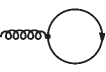
Figure 5.2: Leading order tadpole diagram.

Let us consider the one-loop tadpole diagram as shown in Fig. 5.2,

$$\mathcal{T}^{a}=-{g\over 2}\int{d^{4}Q\over i(2\pi)^{4}}\mathrm{Tr}_{D,c,f,NG}[\hat{\Gamma}_{0}^{a}S(Q)].$$ (5.40)

Here $S(Q)$ is the quark propagator in the Nambu-Gor’kov basis, which is given by Eq. (5.9). At leading order we may neglect the quark self energy $\Sigma$. The quark-gluon vertex $\hat{\Gamma}_{0}^{a}$ is given by

$$\hat{\Gamma}_{0}^{a}=\left(\begin{array}[]{cc}\Gamma_{0}^{a}&0\\ 0&\bar{\Gamma}_{0}^{a}\end{array}\right),$$ (5.41)

with $\Gamma_{0}^{a}=\gamma_{0}T^{a}$ and $\bar{\Gamma}_{0}^{a}=-\gamma_{0}(T^{a})^{T}$. The trace in (5.40) has to be taken with respect to Dirac, color, flavor and Nambu-Gor’kov indices. First we evaluate the trace over Nambu-Gor’kov space which gives

$$\mathcal{T}^{a}=-{g\over 2}\int{d^{4}Q\over i(2\pi)^{4}}\mathrm{Tr}_{D,c,f}[\Gamma_{0}^{a}\mathcal{G}^{+}(Q)+\bar{\Gamma}_{0}^{a}\mathcal{G}^{-}(Q)],$$ (5.42)

where $\mathcal{G}^{\pm}$ is given in Eq. (5.34) for the 2SC phase. Evaluating the trace over flavor and color space we get

$$\mathcal{T}^{a}=g(T^{a})_{33}\int{d^{4}Q\over i(2\pi)^{4}}\mathrm{Tr}_{D}[\gamma_{0}(G^{+}-G^{-}-G_{0}^{+}+G_{0}^{-})].$$ (5.43)

Assuming that $\phi^{-}\simeq 0$ [156] and that $\phi^{+}$ has negligible four-momentum dependence in the vicinity of the quasiparticle pole we obtain

$$\mathcal{T}^{a} \!\simeq\! -4g(T^{a})_{33}\int{d^{4}Q\over i(2\pi)^{4}}\left({\mu-q\over q_{0}^{2}-(\mu-q)^{2}-|\phi^{+}|^{2}}-{\mu-q\over q_{0}^{2}-(\mu-q)^{2}}\right)$$ (5.44)

$$\!\simeq\! {g\over\pi^{2}}(T^{a})_{33}\int_{0}^{\infty}dq\,q^{2}(\mu-q)\left({1\over\sqrt{(\mu-q)^{2}+|\phi^{+}|^{2}}}-{1\over|\mu-q|}\right).\qquad$$

In order to obtain an order of magnitude estimate, we make the approximation $\phi^{+}(q)\simeq\phi^{+}_{0}\Theta(2\mu-q)$ with $\phi^{+}_{0}=const.$ [139]. Then the $q$-integration can be readily performed, with the result

$$\mathcal{T}^{a}\simeq-{2g\over\pi^{2}}(T^{a})_{33}\,\mu\,(\phi_{0}^{+})^{2}\,\mathrm{log}\left({\phi^{+}_{0}\over 2\mu}\right)+{\mathcal{O}}((g\mu\phi_{0}^{+})^{2}),\quad(T^{a})_{33}=-\delta^{a8}/\sqrt{3}.$$ (5.45)

This result is in fact of order $\mu(\phi_{0}^{+})^{2}$, because $\mathrm{log}(\phi_{0}^{+}/(2\mu))$ is of order $1/g$ [see Eq. (5.13)].

5.6.2 Gluon tadpoles for CFL with $m_{s}\neq 0$

We would like to evaluate the gluon tadpole in the CFL phase with a non-vanishing strange quark mass $m_{s}$. The inverse Nambu-Gor’kov propagator takes the same form as in Eq. (5.9) (with $\Sigma\to 0$ at leading order), where the free inverse propagators are now given by

$$([\mathcal{G}^{+}_{0}]^{-1})^{rs}_{ij}=[(\not{Q}+\mu\gamma_{0})(\delta^{rs}-\delta^{r3}\delta^{s3})+(\not{Q}+\mu\gamma_{0}-m_{s})\delta^{r3}\delta^{s3}]\delta_{ij},$$ (5.46)

$$([\mathcal{G}^{-}_{0}]^{-1})^{rs}_{ij}=[(\not{Q}-\mu\gamma_{0})(\delta^{rs}-\delta^{r3}\delta^{s3})+(\not{Q}-\mu\gamma_{0}-m_{s})\delta^{r3}\delta^{s3}]\delta_{ij},\qquad\qquad$$ (5.47)

Again the lower indices are color indices and the upper ones are flavor indices. At finite $m_{s}$ the Dirac structure of the gap is more complicated than in the massless case [180], but for $m_{s}\ll\mu$ we may assume that the additional terms are suppressed at least with $m_{s}/\mu$ [182],

$$[\Phi^{+}]^{rs}_{ij}\simeq\phi^{+}\Lambda^{+}_{\bf q}\gamma_{5}(\delta_{i}^{r}\delta_{j}^{s}-\delta_{j}^{r}\delta_{i}^{s})+\mathcal{O}\left(\frac{m_{s}}{\mu}\right).$$ (5.48)

As usual we have $\Phi^{-}=\gamma_{0}[\Phi^{+}]^{\dagger}\gamma_{0}$. The inverse full quark propagator can be written as

$$[\mathcal{G}^{+}]^{-1}=[\mathcal{G}^{+}_{0}]^{-1}-\Phi^{-}\mathcal{G}^{-}_{0}\Phi^{+}=\left(\begin{array}[]{ccccccccc}b_{1}&&&&b_{2}&&&&b_{3}\\ &b_{4}&&&&&&&\\ &&b_{5}&&&&&&\\ &&&b_{4}&&&&&\\ b_{2}&&&&b_{1}&&&&b_{3}\\ &&&&&b_{5}&&&\\ &&&&&&b_{6}&&\\ &&&&&&&b_{6}&\\ b_{3}&&&&b_{3}&&&&b_{7}\end{array}\right).$$ (5.49)

The nine rows and columns of this matrix correspond to color and flavor indices, namely (color, flavor)=(1,1),(1,2),(1,3),(2,1),(2,2),(2,3),(3,1),(3,2), (3,3). The $b_{i}$ are matrices in Dirac space, given explicitly by

$$b_{1} = \not{Q}+\mu\gamma_{0}+\gamma_{0}\phi^{\dagger}\gamma_{0}[\not{Q}-\mu\gamma_{0}]^{-1}\phi+\gamma_{0}\phi^{\dagger}\gamma_{0}[\not{Q}-\mu\gamma_{0}-m_{s}]^{-1}\phi,$$

$$b_{2} = \gamma_{0}\phi^{\dagger}\gamma_{0}[\not{Q}-\mu\gamma_{0}-m_{s}]^{-1}\phi,$$

$$b_{3} = \gamma_{0}\phi^{\dagger}\gamma_{0}[\not{Q}-\mu\gamma_{0}]^{-1}\phi,$$

$$b_{4} = \not{Q}+\mu\gamma_{0}+\gamma_{0}\phi^{\dagger}\gamma_{0}[\not{Q}-\mu\gamma_{0}]^{-1}\phi,$$

$$b_{5} = \not{Q}+\mu\gamma_{0}-m_{s}+\gamma_{0}\phi^{\dagger}\gamma_{0}[\not{Q}-\mu\gamma_{0}]^{-1}\phi,$$

$$b_{6} = \not{Q}+\mu\gamma_{0}+\gamma_{0}\phi^{\dagger}\gamma_{0}[\not{Q}-\mu\gamma_{0}-m_{s}]^{-1}\phi,$$

$$b_{7} = \not{Q}+\mu\gamma_{0}-m_{s}+2\gamma_{0}\phi^{\dagger}\gamma_{0}[\not{Q}-\mu\gamma_{0}]^{-1}\phi,$$ (5.50)

with $\phi=\phi^{+}\Lambda^{+}_{\bf q}\gamma_{5}$. The full quark propagator is obtained by inverting the matrix in (5.49),

$$\!\!\!\!\!\!\!\mathcal{G}^{+}=\left(\begin{array}[]{ccccccccc}a_{1}&&&&a_{2}&&&&a_{3}\\ &a_{5}&&&&&&&\\ &&a_{6}&&&&&&\\ &&&a_{5}&&&&&\\ a_{2}&&&&a_{1}&&&&a_{3}\\ &&&&&a_{6}&&&\\ &&&&&&a_{7}&&\\ &&&&&&&a_{7}&\\ a_{4}&&&&a_{4}&&&&a_{8}\end{array}\right),\qquad$$ (5.51)

with

$$a_{1} = (b_{1}-b_{2})^{-1}+a_{2},$$

$$a_{2} = (-2b_{3}+b_{7}b_{3}^{-1}(b_{1}+b_{2}))^{-1}(b_{3}-b_{7}b_{3}^{-1}b_{2})(b_{1}-b_{2})^{-1},$$

$$a_{3} = (2b_{3}-b_{7}b_{3}^{-1}(b_{1}+b_{2}))^{-1},$$

$$a_{4} = -b_{3}^{-1}(b_{2}(b_{1}-b_{2})^{-1}+(b_{1}+b_{2})a_{2}),$$

$$a_{5} = b_{4}^{-1},$$

$$a_{6} = b_{5}^{-1},$$

$$a_{7} = b_{6}^{-1},$$

$$a_{8} = -b_{3}^{-1}(b_{1}+b_{2})a_{3}.$$ (5.52)

Similar expressions can be obtained for $\mathcal{G}^{-}:=[[\mathcal{G}^{-}_{0}]^{-1}-\Phi^{+}\mathcal{G}^{+}_{0}\Phi^{-}]^{-1}$.

The gluon tadpole is given by

$$\mathcal{T}^{a}:=-{g\over 2}\int{d^{4}Q\over i(2\pi)^{4}}\mathrm{Tr_{D}}\gamma_{0}\left([\mathcal{G}^{+}]_{ij}^{rs}(T^{a})_{ji}-[\mathcal{G}^{-}]_{ij}^{rs}(T^{a})_{ij}\right)\delta^{rs}.$$ (5.53)

Taking the trace over color and flavor space we find that the only non-vanishing tadpole is $\mathcal{T}^{8}$,

$$\mathcal{T}^{8}=-{g\over 2\sqrt{3}}\int{d^{4}Q\over i(2\pi)^{4}}\mathrm{Tr_{D}}\gamma_{0}(a_{1}+a_{5}+a_{6}-2a_{7}-a_{8})-(\textrm{similar terms from }G^{-}).$$ (5.54)

We perform a Taylor expansion in $m_{s}$, keeping only the leading term which is of order $m_{s}^{2}$. With the approximation $\phi^{-}\simeq 0$ we get

$$\!\!\!\!\!\!\!\!\!\!\!\!\!\!\!\!\!\!\!\!\!\!\mathcal{T}^{a}\simeq\delta^{a8}\frac{gm_{s}^{2}}{2\sqrt{3}\pi^{3}}\int_{-\infty}^{\infty}dq_{4}\int_{0}^{\infty}dq$$

$$\times\frac{q\,(\phi^{+})^{2}\left(q_{4}^{2}-3(q-\mu)^{2}-8(\phi^{+})^{2}\right)}{\left(q_{4}^{2}+(q-\mu)^{2}+(\phi^{+})^{2}\right)^{2}\left(q_{4}^{2}+(q-\mu)^{2}+4(\phi^{+})^{2}\right)}.$$ (5.55)

This integral seems to be proportional to $(\phi^{+})^{2}$. It turns out, however, that the factor $(\phi^{+})^{2}$ cancels against a factor $1/(\phi^{+})^{2}$ from the result of the integration. This is related to the fact that for $\phi^{+}\rightarrow 0$ the integral would contain an infrared singularity, which is regulated by the gap [183].

We make the approximation $\phi^{+}\simeq\phi^{+}_{0}\Theta(2\mu-q)$. After the integration we take the limit $\phi^{+}_{0}\rightarrow 0$, since we assume $m_{s}\gg\phi^{+}_{0}$. This leads to [184]

$$\mathcal{T}^{8}\simeq-\mu m_{s}^{2}{4g\over 9\sqrt{3}\pi^{2}}(21-8\log 2).$$ (5.56)

5.6.3 Color neutrality

To address the question of color neutrality [142, 146, 185, 186, 187, 188] we consider the partition function

$$\exp(-\Omega/T)=\int\mathcal{D}\varphi\,\exp(-S[\varphi]),$$ (5.57)

where $\varphi$ denotes the set of all fields, and $S[\varphi]$ is the QCD action (including gauge fixing terms and ghosts). Following the argument given in [189] it is easy to see that the system described by this partition function is color neutral, at least if one chooses a gauge fixing which does not involve $A_{0}^{a}$, for instance Coulomb gauge: The fields $A_{0}^{a}$ appear in the action as Lagrange multipliers for the Gauss law constraint [190]. Therefore in the path integral the integration over the zero-momentum modes $A_{0,{\bf p}=0}^{a}$ produces delta functions, $\delta(N_{a})$, where $N_{a}$ are the color charges. This means that only color neutral field configurations contribute to the partition function, q.e.d.

The gluon tadpole in the 2SC phase [Eq. (5.45)] induces a non-vanishing expectation value for the gluon field $A_{0}^{8}$,

$$\bar{A}^{0}_{8}\sim m_{D}^{-2}\mu(\phi^{+})^{2}\sim(\phi^{+})^{2}/(g^{2}\mu),\qquad\mathrm{(2SC)}$$ (5.58)

where $m_{D}$ is the corresponding leading-order Debye mass [139]. This expectation value acts as an effective chemical potential for the color number 8,

$$\mu_{8}=g\bar{A}^{0}_{8}\sim(\phi^{+})^{2}/(g\mu).\qquad\mathrm{(2SC)}$$ (5.59)

It may be noted that the chemical potential $\mu_{8}$ which has been found by requiring color neutrality in an NJL model is also proportional to $\phi^{2}$ [187]. In a similar way one finds in the CFL phase from Eq. (5.56)

$$\mu_{8}\sim{m_{s}^{2}/\mu},\qquad\mathrm{(CFL)}$$ (5.60)

which agrees again qualitatively with the result of the NJL model calculation [187]. One should emphasize, however, that whereas in NJL models color neutrality has to be imposed as an additional condition, color neutrality is guaranteed automatically in QCD by the integration over the $A_{0}^{a}$ zero-momentum modes.

The tadpole diagrams we computed above correspond to the first derivative of the effective action at vanishing mean field,

$$\mathcal{T}^{a}\sim\frac{\delta\Gamma}{\delta A_{0}^{a}}\bigg{|}_{A=0}.$$ (5.61)

In [191] the expectation value of $A_{0}^{8}$ is computed self-consistently from the Yang-Mills equation,

$$\frac{\delta\Gamma}{\delta A_{0}^{a}}\bigg{|}_{A=\bar{A}}=0.$$ (5.62)

This approach is completely equivalent to our approach, which can be seen from the Taylor expansion

$$\frac{\delta\Gamma}{\delta A_{0}^{a}}\bigg{|}_{A=0}=\frac{\delta\Gamma}{\delta A_{0}^{a}}\bigg{|}_{A=\bar{A}}-\frac{\delta^{2}\Gamma}{\delta A_{0}^{a}\delta A_{0}^{b}}\bigg{|}_{A=\bar{A}}\bar{A}_{0}^{b}+\ldots$$ (5.63)

On the right hand side the first term vanishes, while the second term is essentially the inverse gluon propagator at zero momentum times the expectation value of $A$.

The tadpole diagram in Fig. 5.2 which we evaluated above corresponds to the fermionic part of the color charge density,

$$\rho^{a}_{(q)}=\sum_{f=1}^{N_{f}}\bar{\psi}_{f}T^{a}\gamma_{0}\psi_{f}.$$ (5.64)

One might ask whether the gluons could also contribute to the charge density. In Ref. [142] it was argued that the gluonic contribution should vanish, since the gluonic part of the charge density

$$\rho^{a}_{(gl)}=f^{abc}A^{b}_{i}F^{c}_{i0}$$ (5.65)

contains the chromoelectric field strength, which vanishes in any (super-)conducting system. The aim of the next subsection is to corroborate this argument by analyzing the tadpole diagram with a gluon loop (Fig. 5.3) [192].

5.6.4 Gluon self energy and gluon loop tadpole (2SC)

Figure 5.3: Tadpole diagram with resummed gluon propagator.

Let us consider the tadpole diagram in Fig. 5.3, where the rhombus indicates a resummed gluon propagator. In [139] integral representations for the various components of the gluon self energy in the 2SC phase have been derived. (The Feynman diagram for the gluon self energy at leading order looks like the second one of Fig. 3.1, with the normal fermion propagators now replaced by Nambu-Gor’kov propagators.) It turns out the the gluon self energy in the 2SC phase has some off-diagonal components with respect to the color indices, therefore the tadpole diagram in Fig. 5.3 does not vanish a priori. The non-vanishing components of the gluon self energy in the 2SC phase are

$$\Pi_{11}=\Pi_{22}=\Pi_{33},\quad\Pi_{44}=\Pi_{55}=\Pi_{66}=\Pi_{77},\quad\Pi_{45}=-\Pi_{54}=\Pi_{67}=-\Pi_{76}.$$ (5.66)

In Ref. [139] the gluon self energy is diagonalized by a unitary transformation in color space. For our purposes it is more convenient not to perform this transformation, since we want to keep the structure constants totally antisymmetric. For the $44$ and $45$ components of the self energy analytical results can be obtained rather easily, as we will demonstrate in the following. We shall always assume that the energy and the momentum of the gluon are much smaller than $\mu$, because if there is any contribution to the tadpole diagrams, it will come from soft gluons. In the notation of Ref. [139] we have

$$\!\!\!\!\!\!\!\!\!\!\!\!\!\!\!\!\!\!\!\!\!\!\Pi_{44}^{00}=-{1\over 2}g^{2}\int{d^{3}k\over(2\pi)^{3}}\sum_{e_{1},e_{2}=\pm}(1+e_{1}e_{2}\,{\bf\hat{k}}_{1}\cdot{\bf\hat{k}}_{2})$$

$$\!\!\!\!\!\!\!\!\!\!\!\!\times\left(n_{1}^{0}(1-n_{2})+(1-n_{1}^{0})n_{2}\right)\left[{1\over p_{0}+\epsilon_{1}^{0}+\epsilon_{2}+i\eta}-{1\over p_{0}-\epsilon_{1}^{0}-\epsilon_{2}+i\eta}\right],$$ (5.67)

and

$$\!\!\!\!\!\!\!\!\!\!\!\!\!\!\!\!\!\!\!\!\!\!-i\Pi_{45}^{00}\equiv\hat{\Pi}^{00}=-{1\over 2}g^{2}\int{d^{3}k\over(2\pi)^{3}}\sum_{e_{1},e_{2}=\pm}(1+e_{1}e_{2}\,{\bf\hat{k}}_{1}\cdot{\bf\hat{k}}_{2})$$

$$\!\!\!\!\!\!\!\!\!\!\!\!\times\left(n_{1}^{0}(1-n_{2})-(1-n_{1}^{0})n_{2}\right)\left[{1\over p_{0}+\epsilon_{1}^{0}+\epsilon_{2}+i\eta}-{1\over p_{0}-\epsilon_{1}^{0}-\epsilon_{2}+i\eta}\right].$$ (5.68)

Here we have used the notations of Ref. [139],

$$\epsilon_{i}=\sqrt{(\mu-e_{i}k_{i})^{2}+|\phi_{i}|^{2}},$$ (5.69)

$$n_{i}={\epsilon_{i}+\mu-e_{i}k_{i}\over 2\epsilon_{i}},$$ (5.70)

where $\phi_{i}\equiv\phi^{e_{i}}(\epsilon_{i},k_{i})$ is the on-shell gap function. The superscript “0” means $\phi_{i}\to 0$. First let us evaluate $\mathrm{Im}\Pi_{44}^{00}$. Without loss of generality we assume $p_{0}>0$. For $p_{0}<\mu$ the only contribution arises from $e_{1}=e_{2}=+$. With ${\bf k}_{1}={\bf k}+{\bf p}$, ${\bf k}_{2}={\bf k}$, ${\bf\hat{k}}\cdot{\bf\hat{p}}=t$, $k_{1}=\sqrt{k^{2}+p^{2}+2pt}$, $\xi=k-\mu$, $\phi:=\phi_{2}$ we find

$$\!\!\!\!\!\!\!\!\mathrm{Im}\Pi_{44}^{00}=-{g^{2}\over 8\pi}\int_{-\mu}^{\infty}d\xi\,(\mu+\xi)^{2}\int_{-1}^{1}dt\,\Theta(p_{0}-\phi)\left(1+{\mu+\xi+pt\over k_{1}}\right)$$

$$\quad\times\Theta\!\left(p_{0}-\sqrt{\xi^{2}+\phi^{2}}\right)\bigg{[}{\sqrt{\xi^{2}+\phi^{2}}+\xi\over 2\sqrt{\xi^{2}+\phi^{2}}}\,\delta\left(p_{0}-\mu+k_{1}-\sqrt{\xi^{2}+\phi^{2}}\right)$$

$$\qquad+{\sqrt{\xi^{2}+\phi^{2}}-\xi\over 2\sqrt{\xi^{2}+\phi^{2}}}\,\delta\left(p_{0}+\mu-k_{1}-\sqrt{\xi^{2}+\phi^{2}}\right)\bigg{]}.$$ (5.71)

Because of the step function in the second line we have $\xi\ll\mu$ for $p_{0}\ll\mu$. Therefore it is sufficient to approximate $\phi$ with its value at the Fermi surface, which we denote with $\phi_{0}$. Rewriting the delta functions as $\delta(t-\ldots)$, we find for $p\ll\mu$

$$\!\!\!\!\!\!\!\!\!\!\!\mathrm{Im}\Pi_{44}^{00}=-\Theta(p_{0}-\phi_{0}){g^{2}\over 16\pi p}\int_{-\sqrt{p_{0}^{2}-\phi_{0}^{2}}}^{\sqrt{p_{0}^{2}-\phi_{0}^{2}}}d\xi\,(\mu+\xi)^{2}\int_{-1}^{1}dt$$

$$\!\!\!\!\!\!\!\!\!\!\times\bigg{[}{\left(\kappa+\xi\right)\left(2\mu-p_{0}+pt+\xi+\kappa\right)\over\kappa\left(\mu+\xi\right)}\Theta\!\left(p+p_{0}+\xi-\kappa\right)\Theta\!\left(p-p_{0}-\xi+\kappa\right)\delta(t-{\bar{t}}_{1})$$

$$\!\!\!\!\!\!\!\!\!+{\left(\kappa-\xi\right)\left(2\mu+p_{0}+pt+\xi-\kappa\right)\over\kappa\left(\mu+\xi\right)}\Theta\!\left(p+p_{0}-\xi-\kappa\right)\Theta\!\left(p-p_{0}+\xi+\kappa\right)\delta(t-{\bar{t}}_{2})\bigg{]}$$

with $\kappa=\sqrt{\xi^{2}+\phi_{0}^{2}}$ and

$${\bar{t}}_{1}={2\mu\left(-p_{0}-\xi+\kappa\right)+\phi_{0}^{2}-p^{2}+p_{0}^{2}-2p_{0}\kappa\over 2p(\mu+\xi)},$$ (5.73)

$${\bar{t}}_{2}={2\mu\left(p_{0}-\xi-\kappa\right)+\phi_{0}^{2}-p^{2}+p_{0}^{2}-2p_{0}\kappa\over 2p(\mu+\xi)}.$$ (5.74)

We make the substitution $\xi\to-\xi$ in the term with ${\bar{t}}_{1}$, which leads to

$$\!\!\!\!\!\!\!\!\mathrm{Im}\Pi_{44}^{00}=-\Theta(p_{0}-\phi_{0}){g^{2}\over 16\pi p}\int_{-\sqrt{p_{0}^{2}-\phi_{0}^{2}}}^{\sqrt{p_{0}^{2}-\phi_{0}^{2}}}d\xi\,\Theta\!\left(p+p_{0}-\xi-\kappa\right)\Theta\!\left(p-p_{0}+\xi+\kappa\right)$$

$$\times{1\over\kappa}\left[(4\mu^{2}-p^{2}+(p_{0}+2\xi)^{2})(-\xi+\kappa)-\phi_{0}^{2}(2p_{0}+3\xi-\kappa)\right].$$ (5.75)

The $\xi$-integration is now straightforward, and we find

$$\!\!\!\!\!\!\!\!\!\!\!\!\!\!\!\!\!\!\!\mathrm{Im}\Pi_{44}^{00}=-\Theta(p_{0}-\phi_{0})\Theta(-p_{0}+\sqrt{p^{2}+\phi_{0}^{2}})$$

$$\qquad\times{g^{2}\over 24\pi p}\sqrt{p_{0}^{2}-\phi_{0}^{2}}\left(12\mu^{2}-3p^{2}+p_{0}^{2}-\phi_{0}^{2}\right)$$

$$\quad-\Theta(p_{0}-\sqrt{p^{2}+\phi_{0}^{2}}){g^{2}\mu^{2}\phi_{0}^{2}\over 2\pi(p_{0}^{2}-p^{2})}$$

$$\qquad\times\left[1+{-6\phi_{0}^{2}p_{0}^{2}(p_{0}^{2}-p^{2})+3(p_{0}^{2}-p^{2})^{3}+\phi_{0}^{4}(p^{2}+3p_{0}^{2})\over 12\mu^{2}(p_{0}^{2}-p^{2})^{2}}\right].$$ (5.76)

This result is a generalization of the one-loop gluon self energy at zero temperature in the normal phase given in [77] (see also Sec. 3.2). As in the normal phase, the leading part of the gluon self energy is of the order $g^{2}\mu^{2}$ (for $p_{0},p\ll\mu$). In order to maintain consistency in the following, we shall keep only these leading terms, since contributions from lower powers of $\mu$ might mix with contributions from diagrams with a higher number of loops. Denoting this approximation with a tilde, we have

$$\mathrm{Im}\tilde{\Pi}_{44}^{00}=-\Theta(p_{0}-\phi_{0}){g^{2}\mu^{2}\over 2\pi}\bigg{[}\Theta(-p_{0}+\sqrt{p^{2}+\phi_{0}^{2}}){\sqrt{p_{0}^{2}-\phi_{0}^{2}}\over p}$$

$$\quad\qquad\qquad+\Theta(p_{0}-\sqrt{p^{2}+\phi_{0}^{2}}){\phi_{0}^{2}\over p_{0}^{2}-p^{2}}\bigg{]}.$$ (5.77)

In the following we will refer to this analogon of the HDL approximation as the “leading order” approximation. $\mathrm{Im}\Pi^{00}_{44}$ is an odd function of $p_{0}$, therefore the real part can be calculated with the following dispersion relation [167]

$$\mathrm{Re}\tilde{\Pi}_{44}^{00}(p_{0},p)={1\over\pi}{\mathcal{P}}\int_{0}^{\infty}d\omega\,\mathrm{Im}\tilde{\Pi}_{44}^{00}(\omega,p)\left({1\over\omega+p_{0}}+{1\over\omega-p_{0}}\right).$$ (5.78)

In contrast to the $11$, $22$, $33$ and $88$ components of the gluon self energy, the principal value integral can be performed analytically in this case,

$$\!\!\!\!\!\!\!\!\!\!\!\!\!\!\!\!\!\!\!\!\mathrm{Re}\tilde{\Pi}_{44}^{00}=-{g^{2}\mu^{2}\over\pi^{2}}\Bigg{[}\Theta\left(\phi_{0}^{2}-p_{0}^{2}\right)\left(1-{\sqrt{\phi_{0}^{2}-p_{0}^{2}}\over p}\arctan{p\over\sqrt{\phi_{0}^{2}-p_{0}^{2}}}\right)$$

$$+\Theta\left(p_{0}^{2}-\phi_{0}^{2}\right)\left(1+{\sqrt{p_{0}^{2}-\phi_{0}^{2}}\over 2p}\log\bigg{|}{\sqrt{p_{0}^{2}-\phi_{0}^{2}}-p\over\sqrt{p_{0}^{2}-\phi_{0}^{2}}+p}\bigg{|}\right)$$

$$+{\phi_{0}^{2}\over 2(p^{2}-p_{0}^{2})}\log\bigg{|}{\phi_{0}^{2}+p^{2}-p_{0}^{2}\over\phi_{0}^{2}}\bigg{|}\Bigg{]}.$$ (5.79)

As a consistency check, we may extract the Debye mass in the normal and in the superconducting phase,

$$-\lim_{p\to 0}\lim_{p_{0}\to 0}\lim_{\phi_{0}\to 0}\mathrm{Re}\tilde{\Pi}_{44}^{00}(p_{0},p)\!\!\! = \!\!\!{g^{2}\mu^{2}\over\pi^{2}},$$ (5.80)

$$-\lim_{p\to 0}\lim_{p_{0}\to 0}\mathrm{Re}\tilde{\Pi}_{44}^{00}(p_{0},p)\!\!\! = \!\!\!{g^{2}\mu^{2}\over 2\pi^{2}},$$ (5.81)

which are the standard results for $N_{f}=2$ [139]. For the other Lorentz components of the self energy one finds following the same steps as above

$$\!\!\!\!\!\!\!\!\mathrm{Im}\tilde{\Pi}_{44}^{0i}=-\Theta(p_{0}-\phi_{0}){g^{2}\mu^{2}\over 4\pi p^{2}}\hat{p}^{i}\bigg{[}\Theta(p-\upsilon)\left(2p_{0}\upsilon+\phi_{0}^{2}\log{p_{0}-\upsilon\over p_{0}+\upsilon}\right)$$

$$\ \qquad\qquad+\Theta(\upsilon-p)\,\phi_{0}^{2}\left({2pp_{0}\over p_{0}^{2}-p^{2}}+\log{p_{0}-p\over p_{0}+p}\right)\bigg{]},$$ (5.82)

$$\!\!\!\!\!\!\!\!\mathrm{Im}\tilde{\Pi}_{44}^{ij}=\Theta(p_{0}-\phi_{0}){g^{2}\mu^{2}\over 4\pi p^{3}}$$

$$\times\bigg{[}(\delta^{ij}-\hat{p}^{i}\hat{p}^{j})\bigg{(}\Theta(p-\upsilon)\left(\upsilon(p_{0}^{2}-p^{2}+\phi_{0}^{2})+\phi_{0}^{2}p_{0}\log{p_{0}-\upsilon\over p_{0}+\upsilon}\right)$$

$$\qquad+\Theta(\upsilon-p)\phi_{0}^{2}\left(2p+p_{0}\log{p_{0}-p\over p_{0}+p}\right)\bigg{)}$$

$$\quad-2\hat{p}^{i}\hat{p}^{j}\bigg{(}\Theta(p-\upsilon)\left(\upsilon(p_{0}^{2}+\phi_{0}^{2})+\phi_{0}^{2}p_{0}\log{p_{0}-\upsilon\over p_{0}+\upsilon}\right)$$

$$\qquad+\Theta(\upsilon-p)\phi_{0}^{2}\left({(2p_{0}^{2}-p^{2})p\over p_{0}^{2}-p^{2}}+p_{0}\log{p_{0}-p\over p_{0}+p}\right)\bigg{)}\bigg{]},$$ (5.83)

where $\upsilon=\sqrt{p_{0}^{2}-\phi_{0}^{2}}$. Again the real parts could be obtained analytically via dispersion relations, but the resulting expressions are rather unwieldy and we shall refrain from writing them down here.

The off-diagonal components of the gluon self energy can be evaluated in an analogous way. In place of Eq. (5.75) we find

$$\!\!\!\!\!\!\!\!\mathrm{Im}\hat{\Pi}^{00}=-\Theta(p_{0}-\phi_{0}){g^{2}\over 4\pi p}\int_{-\sqrt{p_{0}^{2}-\phi_{0}^{2}}}^{\sqrt{p_{0}^{2}-\phi_{0}^{2}}}d\xi\,\Theta\!\left(p+p_{0}-\xi-\kappa\right)\Theta\!\left(p-p_{0}+\xi+\kappa\right)$$

$$\times{\mu\over\kappa}\left(\phi_{0}^{2}-(p_{0}+2\xi)(\kappa-\xi)\right),$$ (5.84)

which gives

$$\mathrm{Im}\hat{\Pi}^{00}=-\Theta(p_{0}-\sqrt{p^{2}+\phi_{0}^{2}})g^{2}\mu{p_{0}\phi_{0}^{2}(\phi_{0}^{2}+p^{2}-p_{0}^{2})\over 2\pi(p_{0}^{2}-p^{2})^{2}}.$$ (5.85)

We observe that in this one-loop result there is a term which is linear in $\mu$, but there is no term of order $g^{2}\mu^{2}$. Therefore we have at our order of accuracy

$$\mathrm{Im}\tilde{\hat{\Pi}}^{\raisebox{-5.0pt}{\scriptsize{00}}}=0.$$ (5.86)

In fact this can be seen rather directly from the ($e_{1}=e_{2}=+$)-component of Eq. (5.68): if we set $d^{3}k\to 2\pi\mu^{2}d\xi dt$ we find at the order $g^{2}\mu^{2}$ that the integrand is odd with respect to $\xi\to-\xi$, $t\to-t$, and therefore the integral vanishes at this order. This argument also holds for the real part, $\mathrm{Re}\tilde{\hat{\Pi}}^{\raisebox{-5.0pt}{\scriptsize{00}}}=0$. In the same way it can be shown that $\tilde{\hat{\Pi}}^{\raisebox{-5.0pt}{\scriptsize{0i}}}=0$ and $\tilde{\hat{\Pi}}^{\raisebox{-5.0pt}{\scriptsize{ij}}}=0$.

This implies that the resummed gluon propagator is diagonal in the color indices at leading order. Since the three-gluon vertex is antisymmetric in the color indices at tree level, we conclude that the tadpole diagram of Fig. (5.3) vanishes at the order of our computation. This means that at this order the expectation value of the gluon field, Eq. (5.58), is not changed by the tadpole diagram in Fig. (5.3). Therefore the effective chemical potential is determined completely by the quark part of the color charge density at the order of our computation, whereas the gluonic part is negligible at this order.

We note that there is no contribution from the tadpole diagram with a ghost loop. The reason is that there is no direct coupling between quarks and ghosts in the QCD Lagrangian, therefore the ghost self energy vanishes at the order $g^{2}\mu^{2}$, and the ghost propagator is proportional to the unit matrix in color space at leading order. Furthermore we remark that e.g. in covariant or Coulomb gauge in particular the gauge dependent part of the gluon propagator is diagonal in the color indices at leading order. Therefore the effective chemical potential is gauge independent at this order.

5.6.5 Gluon vertex correction (2SC)

Figure 5.4: Tadpole diagram with resummed gluon propagator and three-gluon vertex correction.

We would like to check whether the above result is modified if one replaces the tree level gluon vertex with the one-loop vertex correction, as shown in Fig. 5.4. We remark that the tadpole diagram in Fig. 5.4 corresponds to a higher order correction to the fermionic part of the charge density [Eq. (5.64)]. Let us evaluate the one-loop three-gluon vertex of Fig. 5.4 in the limit where one of the gluon momenta approaches zero. After taking the trace with respect to Nambu-Gor’kov, color and flavor indices we find

$$\!\!\!\!\!\!\!\!\!\!\!\!\!\!\!\!\!\!\!\!\!\Gamma_{485}^{\mu 0\nu}=-{ig^{3}\over\sqrt{3}}\int{d^{4}K\over i(2\pi)^{4}}\mathrm{Tr}_{D}\bigg{[}-\gamma^{\mu}G^{+}(K_{1})\gamma^{0}G^{+}(K_{1})\gamma^{\nu}G_{0}^{+}(K_{2})$$

$$-2\gamma^{\mu}G_{0}^{+}(K_{1})\gamma^{0}G_{0}^{+}(K_{1})\gamma^{\nu}G^{+}(K_{2})-\gamma^{\mu}G^{-}(K_{1})\gamma^{0}G^{-}(K_{1})\gamma^{\nu}G_{0}^{-}(K_{2})$$

$$-2\gamma^{\mu}G_{0}^{-}(K_{1})\gamma^{0}G_{0}^{-}(K_{1})\gamma^{\nu}G^{-}(K_{2})+\gamma^{\mu}\Xi^{+}(K_{1})\gamma^{0}\Xi^{-}(K_{1})\gamma^{\nu}G_{0}^{-}(K_{2})$$

$$+\gamma^{\mu}\Xi^{-}(K_{1})\gamma^{0}\Xi^{+}(K_{1})\gamma^{\nu}G_{0}^{+}(K_{2})\bigg{]},$$ (5.87)

$$\!\!\!\!\!\!\!\!\!\!\!\!\!\!\!\!\!\!\!\!\!\Gamma_{181}^{\mu 0\nu}=-{2g^{3}\over\sqrt{3}}\int{d^{4}K\over i(2\pi)^{4}}\mathrm{Tr}_{D}\bigg{[}\gamma^{\mu}G^{+}(K_{1})\gamma^{0}G^{+}(K_{1})\gamma^{\nu}G^{+}(K_{2})$$

$$-\gamma^{\mu}G^{-}(K_{1})\gamma^{0}G^{-}(K_{1})\gamma^{\nu}G^{-}(K_{2})+\gamma^{\mu}\Xi^{+}(K_{1})\gamma^{0}\Xi^{-}(K_{1})\gamma^{\nu}G^{-}(K_{2})$$

$$-\gamma^{\mu}\Xi^{-}(K_{1})\gamma^{0}\Xi^{+}(K_{1})\gamma^{\nu}G^{+}(K_{2})+\gamma^{\mu}\Xi^{+}(K_{1})\gamma^{0}G^{+}(K_{1})\gamma^{\nu}\Xi^{-}(K_{2})$$

$$-\gamma^{\mu}\Xi^{-}(K_{1})\gamma^{0}G^{-}(K_{1})\gamma^{\nu}\Xi^{+}(K_{2})-\gamma^{\mu}G^{-}(K_{1})\gamma^{0}\Xi^{+}(K_{1})\gamma^{\nu}\Xi^{-}(K_{2})$$

$$+\gamma^{\mu}G^{+}(K_{1})\gamma^{0}\Xi^{-}(K_{1})\gamma^{\nu}\Xi^{+}(K_{2})\bigg{]},$$ (5.88)

$$\!\!\!\!\!\!\!\!\!\!\!\!\!\!\!\!\!\!\!\!\!\Gamma_{484}^{\mu 0\nu}=-{g^{3}\over\sqrt{3}}\int{d^{4}K\over i(2\pi)^{4}}\mathrm{Tr}_{D}\bigg{[}\gamma^{\mu}G^{+}(K_{1})\gamma^{0}G^{+}(K_{1})\gamma^{\nu}G_{0}^{+}(K_{2})$$

$$-2\gamma^{\mu}G_{0}^{+}(K_{1})\gamma^{0}G_{0}^{+}(K_{1})\gamma^{\nu}G^{+}(K_{2})-\gamma^{\mu}G^{-}(K_{1})\gamma^{0}G^{-}(K_{1})\gamma^{\nu}G_{0}^{-}(K_{2})$$

$$+2\gamma^{\mu}G_{0}^{-}(K_{1})\gamma^{0}G_{0}^{-}(K_{1})\gamma^{\nu}G^{-}(K_{2})+\gamma^{\mu}\Xi^{+}(K_{1})\gamma^{0}\Xi^{-}(K_{1})\gamma^{\nu}G_{0}^{-}(K_{2})$$

$$-\gamma^{\mu}\Xi^{-}(K_{1})\gamma^{0}\Xi^{+}(K_{1})\gamma^{\nu}G_{0}^{+}(K_{2})\bigg{]},$$ (5.89)

$$\!\!\!\!\!\!\!\!\!\!\!\!\!\!\!\!\!\!\!\!\!\Gamma_{888}^{\mu 0\nu}=-{2g^{3}\over 3\sqrt{3}}\int{d^{4}K\over i(2\pi)^{4}}\mathrm{Tr}_{D}\bigg{[}\gamma^{\mu}G^{+}(K_{1})\gamma^{0}G^{+}(K_{1})\gamma^{\nu}G^{+}(K_{2})$$

$$-4\gamma^{\mu}G_{0}^{+}(K_{1})\gamma^{0}G_{0}^{+}(K_{1})\gamma^{\nu}G_{0}^{+}(K_{2})-\gamma^{\mu}G^{-}(K_{1})\gamma^{0}G^{-}(K_{1})\gamma^{\nu}G^{-}(K_{2})$$

$$+4\gamma^{\mu}G_{0}^{-}(K_{1})\gamma^{0}G_{0}^{-}(K_{1})\gamma^{\nu}G_{0}^{-}(K_{2})+\gamma^{\mu}\Xi^{+}(K_{1})\gamma^{0}\Xi^{-}(K_{1})\gamma^{\nu}G^{-}(K_{2})$$

$$-\gamma^{\mu}\Xi^{-}(K_{1})\gamma^{0}\Xi^{+}(K_{1})\gamma^{\nu}G^{+}(K_{2})-\gamma^{\mu}\Xi^{+}(K_{1})\gamma^{0}G^{+}(K_{1})\gamma^{\nu}\Xi^{-}(K_{2})$$

$$+\gamma^{\mu}\Xi^{-}(K_{1})\gamma^{0}G^{-}(K_{1})\gamma^{\nu}\Xi^{+}(K_{2})+\gamma^{\mu}G^{-}(K_{1})\gamma^{0}\Xi^{+}(K_{1})\gamma^{\nu}\Xi^{-}(K_{2})$$

$$-\gamma^{\mu}G^{+}(K_{1})\gamma^{0}\Xi^{-}(K_{1})\gamma^{\nu}\Xi^{+}(K_{2})\bigg{]},$$ (5.90)

where $K_{1}=K+P$ and $K_{2}=K$. Furthermore one finds the relations

$$\!\!\!\!\!\!\!\!\!\!\!\!\!\!\!\!\!\!\Gamma_{485}=-\Gamma_{584}=\Gamma_{687}=-\Gamma_{786},\quad\Gamma_{181}=\Gamma_{282}=\Gamma_{383},$$

$$\Gamma_{484}=\Gamma_{585}=\Gamma_{686}=\Gamma_{787}.$$ (5.91)

The propagators $G^{\pm}$ and $G^{\pm}_{0}$ in Eqs. (5.87)-(5.90) are defined in Eqs. (5.35) and (5.36), and $\Xi^{\pm}$ is given by [139]

$$\Xi^{+}(K)=-\sum_{h=r,l}\sum_{e=\pm}{\phi^{e}_{h}(K)\over k_{0}^{2}-(\mu-ek)^{2}-|\phi_{h}^{e}|^{2}}\mathcal{P}_{-h}\Lambda^{-e}_{\bf k},$$ (5.92)

$$\Xi^{-}(K)=-\sum_{h=r,l}\sum_{e=\pm}{[\phi^{e}_{h}(K)]^{*}\over k_{0}^{2}-(\mu-ek)^{2}-|\phi_{h}^{e}|^{2}}\mathcal{P}_{h}\Lambda^{e}_{\bf k}.$$ (5.93)

(In the following we will assume again $|\phi_{r}^{e}|=|\phi_{l}^{e}|=\phi^{e}$ [139].) In order to evaluate Eqs. (5.87)-(5.90) we need the following Dirac traces,

$$T_{(1)}^{\mu\nu} = \mathrm{Tr}_{D}\left[\gamma^{\mu}\Lambda^{e_{1}}_{{\bf k}_{1}}\gamma^{0}\gamma^{0}\Lambda^{e_{2}}_{{\bf k}_{1}}\gamma^{0}\gamma^{\nu}\Lambda^{e_{3}}_{{\bf k}_{2}}\gamma^{0}\right],$$ (5.94)

$$T_{(2)}^{\mu\nu} = \mathrm{Tr}_{D}\left[\gamma^{\mu}\mathcal{P}_{-h_{1}}\Lambda^{-e_{1}}_{{\bf k}_{1}}\gamma^{0}\mathcal{P}_{h_{2}}\Lambda^{e_{2}}_{{\bf k}_{1}}\gamma^{\nu}\Lambda^{-e_{3}}_{{\bf k}_{2}}\gamma^{0}\right],$$ (5.95)

$$T_{(3)}^{\mu\nu} = \mathrm{Tr}_{D}\left[\gamma^{\mu}\mathcal{P}_{-h_{1}}\Lambda^{-e_{1}}_{{\bf k}_{1}}\gamma^{0}\Lambda^{e_{2}}_{{\bf k}_{1}}\gamma^{0}\gamma^{\nu}\mathcal{P}_{h_{2}}\Lambda^{e_{3}}_{{\bf k}_{2}}\right],$$ (5.96)

$$T_{(4)}^{\mu\nu} = \mathrm{Tr}_{D}\left[\gamma^{\mu}\Lambda^{e_{1}}_{{\bf k}_{1}}\gamma^{0}\gamma^{0}\mathcal{P}_{h_{1}}\Lambda^{e_{2}}_{{\bf k}_{1}}\gamma^{\nu}\mathcal{P}_{-h_{2}}\Lambda^{-e_{3}}_{{\bf k}_{2}}\right].$$ (5.97)

One finds

$$T^{00}_{(1)}=\delta_{e_{1}e_{2}}\left(1+e_{1}e_{3}{\bf\hat{k}}_{1}\cdot{\bf\hat{k}}_{2}\right),$$ (5.98)

$$T^{0i}_{(1)}=T^{io}_{(1)}=\delta_{e_{1}e_{2}}\left(e_{1}{\hat{k}}^{i}_{1}+e_{3}{\hat{k}}^{i}_{2}\right),$$ (5.99)

$$T^{ij}_{(1)}=\delta_{e_{1}e_{2}}\left[\delta^{ij}\left(1-e_{1}e_{3}{\bf\hat{k}}_{1}\cdot{\bf\hat{k}}_{2}\right)+e_{1}e_{3}\left(\hat{k}^{i}_{1}\hat{k}^{j}_{2}+\hat{k}^{i}_{2}\hat{k}^{j}_{1}\right)\right].$$ (5.100)

$T_{(2)}$,$T_{(3)}$ and $T_{(4)}$ contain a common factor ${1\over 2}\delta_{h_{1}h_{2}}$, which we do not write in the following. Then we find

$$T^{00}_{(1)}=T^{00}_{(2)}=T^{00}_{(3)}=T^{00}_{(4)},$$ (5.101)

$$T^{0i}_{(1)}=-T^{0i}_{(2)}=T^{0i}_{(3)}=-T^{0i}_{(4)},$$ (5.102)

$$T^{i0}_{(1)}=T^{i0}_{(2)}=-T^{i0}_{(3)}=T^{i0}_{(4)},$$ (5.103)

$$T^{ij}_{(1)}=T^{ij}_{(2)}=-T^{ij}_{(3)}=-T^{ij}_{(4)}.$$ (5.104)

After performing the energy integration one finds for instance

$$\!\!\!\!\!\!\!\!\!\Gamma^{000}_{485}(P,0,-P)={ig^{3}\over 2\sqrt{3}}\int{d^{3}k\over(2\pi)^{3}}\sum_{e_{1},e_{2}=\pm}(1+e_{1}e_{2}\,{\bf\hat{k}}_{1}\cdot{\bf\hat{k}}_{2})$$

$$\!\!\!\!\!\times\bigg{[}\bigg{(}{1\over\left(p_{0}-\epsilon_{1}-\epsilon_{2}^{0}+i\eta\right)^{2}}+{1\over\left(p_{0}+\epsilon_{1}+\epsilon_{2}^{0}+i\eta\right)^{2}}\bigg{)}{2\phi_{1}^{2}+3\xi_{1}^{2}-3\xi_{1}\epsilon_{1}\mathrm{sgn}(\xi_{2})\over\epsilon_{1}^{2}}$$

$$\ \ +\bigg{(}{1\over p_{0}-\epsilon_{1}-\epsilon_{2}^{0}+i\eta}-{1\over p_{0}+\epsilon_{1}+\epsilon_{2}^{0}+i\eta}\bigg{)}{\phi_{1}^{2}\over\epsilon_{1}^{3}}\bigg{]},$$ (5.105)

$$\!\!\!\!\!\!\!\!\!\Gamma^{000}_{484}(P,0,-P)=-{g^{3}\over 2\sqrt{3}}\int{d^{3}k\over(2\pi)^{3}}\sum_{e_{1},e_{2}=\pm}(1+e_{1}e_{2}\,{\bf\hat{k}}_{1}\cdot{\bf\hat{k}}_{2})$$

$$\!\!\!\!\!\times\bigg{[}\bigg{(}{1\over\left(p_{0}-\epsilon_{1}-\epsilon_{2}^{0}+i\eta\right)^{2}}+{1\over\left(p_{0}+\epsilon_{1}+\epsilon_{2}^{0}+i\eta\right)^{2}}\bigg{)}{-\mathrm{sgn}(\xi_{2})(2\phi_{1}^{2}+3\xi_{1}^{2})+3\xi_{1}\epsilon_{1}\over\epsilon_{1}^{2}}$$

$$\ \ -\bigg{(}{1\over p_{0}-\epsilon_{1}-\epsilon_{2}^{0}+i\eta}-{1\over p_{0}+\epsilon_{1}+\epsilon_{2}^{0}+i\eta}\bigg{)}{\mathrm{sgn}(\xi_{2})\phi_{1}^{2}\over\epsilon_{1}^{3}}\bigg{]},$$ (5.106)

where ${\bf k}_{1}={\bf k}+{\bf p}$, ${\bf k}_{2}={\bf k}$, and $\xi_{i}=e_{i}k_{i}-\mu$. The integrals can be evaluated in a similar way as in the previous section. It is easy to see that $\Gamma^{\mu 0\nu}_{484}(P,0,-P)$ vanishes at the order $g^{3}\mu^{2}$. In general (see also [140]) one finds that $\Gamma^{\mu 0\nu}_{abc}(P,0,-P)$ is non-vanishing at the order $g^{3}\mu^{2}$ only for those combinations of color indices where $f_{abc}$ is non-vanishing. In the previous section we have seen that the gluon propagator is diagonal in the color indices at leading order. Therefore the tadpole diagram in Fig. 5.4 also vanishes at this order.

5.6.6 Mixing with Nambu-Goldstone bosons (2SC)

The symmetry breaking pattern of the 2SC phase is $SU(3)_{c}\times U(1)_{B}\to SU(2)\times\tilde{U}(1)_{B}$ [39]. Therefore five massless (would-be) Nambu-Goldstone (NG) bosons appear in this phase, which correspond to fluctuations of the diquark condensate. As shown in [136, 137, 138], one finds the following effective action for gluons, ghosts and NG bosons after integrating out the quarks,

$$\!\!\!\!\!\!\!\!\Gamma=\int d^{4}x\,\mathcal{L}_{\mathrm{(g)}}+{1\over 2}\mathrm{Tr}\log\left({\mathcal{S}}^{-1}+\gamma_{\mu}\Omega^{\mu}\right)$$

$$=\int d^{4}x\,\mathcal{L}_{\mathrm{(g)}}+{1\over 2}\mathrm{Tr}\log{\mathcal{S}}^{-1}+{1\over 2}\mathrm{Tr}\left({\mathcal{S}}\gamma_{\mu}\Omega^{\mu}\right)-{1\over 4}\mathrm{Tr}\left({\mathcal{S}}\gamma_{\mu}\Omega^{\mu}{\mathcal{S}}\gamma_{\nu}\Omega^{\nu}\right)$$

$$\quad+{1\over 6}\mathrm{Tr}\left({\mathcal{S}}\gamma_{\mu}\Omega^{\mu}{\mathcal{S}}\gamma_{\nu}\Omega^{\nu}{\mathcal{S}}\gamma_{\rho}\Omega^{\rho}\right)+\ldots,{}$$ (5.107)

where the gluonic part of the Lagrangian is e.g. in covariant gauge given by

$$\mathcal{L}_{\mathrm{(g)}}=-{1\over 4}F_{\mu\nu}^{a}F^{\mu\nu a}+{1\over 2\lambda}(\partial^{\mu}A_{\mu}^{a})^{2}-\bar{c}^{a}\partial^{\mu}D_{\mu}^{ab}c^{b},$$ (5.108)

where $F^{\mu\nu}_{a}$ is the usual field strength of the gluons, $c$ and $\bar{c}$ are the (anti-)ghost fields, and $D_{\mu}^{ab}$ is the covariant derivative in the adjoint representation (see e.g. [190]). The quark propagator $S$ reads, in the notation of Ref. [138],

$$S=\left(\begin{array}[]{cc}[G_{0}^{+}]^{-1}&\Phi^{-}\\ \Phi^{+}&[G_{0}^{-}]^{-1}\end{array}\right)^{-1},$$ (5.109)

and $\Omega_{\mu}$ is given by

$$\Omega^{\mu}(x,y)=-i\left(\begin{array}[]{cc}\omega^{\mu}(x)&0\\ 0&-(\omega^{\mu})^{T}(x)\end{array}\right)\delta^{4}(x-y).$$ (5.110)

Here $\omega^{\mu}$ is the (Lie algebra valued) Maurer-Cartan one-form introduced in [136],

$$\omega^{\mu}={\mathcal{V}}^{\dagger}\left(i\partial^{\mu}+gA_{a}^{\mu}T_{a}\right){\mathcal{V}},$$ (5.111)

where

$${\mathcal{V}}=\exp\left[i\left(\sum_{a=4}^{7}\varphi_{a}T_{a}+{1\over\sqrt{3}}\varphi_{8}B\right)\right]$$ (5.112)

parametrizes the coset space $SU(3)_{c}\times U(1)_{B}/SU(2)\times\tilde{U}(1)_{B}$ [137], $B=({\bf 1}+\sqrt{3}T_{8})/3$ is a generator orthogonal to the one of $\tilde{U}(1)_{B}$, and $\varphi_{a}$ are the NG bosons. We may expand $\omega^{\mu}$ in powers of the fields,

$$\!\!\!\!\!\!\!\!\!\!\omega^{\mu}=-{1\over\sqrt{3}}\partial^{\mu}\varphi_{8}B+\bigg{[}gA^{\mu}_{a}-\partial^{\mu}\tilde{\varphi}_{a}-gf_{abc}A^{\mu}_{b}\tilde{\varphi}_{c}-{g\over 3}f_{ab8}A^{\mu}_{b}\varphi_{8}-{1\over 2}f_{abc}\tilde{\varphi}_{b}\partial^{\mu}\tilde{\varphi}_{c}$$

$$\qquad-{1\over 6}f_{a8c}\varphi_{8}\partial^{\mu}\tilde{\varphi}_{c}-{1\over 6}f_{ab8}\tilde{\varphi}_{b}\partial^{\mu}\varphi_{8}+\ldots\bigg{]}T_{a}$$ (5.113)

where $\tilde{\varphi}_{a}\equiv\varphi_{a}$ for $a=4,5,6,7$ and $\tilde{\varphi}_{a}\equiv 0$ otherwise.

Let us examine the various terms in the effective action (5.107). First consider the term linear in $\Omega$, which contains the one-loop gluon tadpole (Fig. 5.2). In principle this term also gives contributions to higher $n$-point functions, since $\Omega$ contains arbitrarily high powers of $\varphi$. In particular, there is a contribution to the bosonic self energy, but this effect is negligible at leading order since the one-loop tadpole [Eq. (5.45)] is only linear in $\mu$.

The term quadratic in $\Omega$ contains the bosonic self energy. As in section 5.6.5 one finds that at leading order the self energy is diagonal in the color indices. There are mixed terms between gluons and NG bosons, which could be eliminated by choosing a suitable t’Hooft gauge [138]. This is not necessary for our purposes, but we note that choosing this t’Hooft gauge would not alter our conclusion, since also in the t’Hooft gauge of Ref. [138] the gluon, NG and ghost propagators are diagonal in the color indices at leading order. The gluon and NG propagators in the t’Hooft gauge are given explicitly in Eqs. (54) and (55) of Ref. [138]. At leading order the propagators (and in particular the gauge dependent parts of the propagators) are diagonal in the color indices also without the unitary transformation in color space that is employed in Ref. [138].

The term quadratic in $\Omega$ also contains new types of three-boson vertices proportional to $f_{abc}$, which involve at least one NG boson.

The term cubic in $\Omega$ is only non-vanishing at the order $g^{3}\mu^{2}$ for those color indices where $f_{abc}\neq 0$. In this thesis we do not consider vertices with more than three legs, since these would appear only in two-loop tadpole diagrams.

To summarize, we find at leading order as in the previous subsections that the bosonic propagators are diagonal in the color indices, and that three-boson vertices of the type $V^{\mu 0\nu}_{abc}(P,0,-P)$ are non-zero only for those combinations of color indices where $f_{abc}\neq 0$. We conclude that the tadpole diagram in Fig. (5.4) vanishes at the order of our computation, even if we take into account NG bosons.

5.6.7 Tadpoles with bosonic loops in the CFL phase

In the case $m_{s}=0$ the situation for the diagrams in Figs. (5.3), (5.4) is similar to the 2SC phase. In the CFL phase the one-loop gluon self energy is proportional to the unit matrix in color space [128] (as in the normal phase). Therefore the diagram in Fig. 5.3 vanishes identically. For the gluon vertex correction one finds after taking the trace with respect to Nambu-Gor’kov, color and flavor indices

$$\!\!\!\!\!\!\!\!\!\!\!\!\!\!\!\Gamma^{\mu 0\nu}_{abc}(P,0,-P)=-{g^{3}\over 24}\int{d^{4}K\over i(2\pi)^{4}}\mathrm{Tr}_{D}\bigg{\{}if_{abc}\bigg{[}\gamma^{\mu}G_{1}^{+}(K_{1})\gamma^{0}G_{2}^{+}(K_{1})\gamma^{\nu}G_{2}^{+}(K_{2})$$

$$+\gamma^{\mu}G_{1}^{-}(K_{1})\gamma^{0}G_{2}^{-}(K_{1})\gamma^{\nu}G_{2}^{-}(K_{2})+\gamma^{\mu}G_{2}^{+}(K_{1})\gamma^{0}G_{1}^{+}(K_{1})\gamma^{\nu}G_{2}^{+}(K_{2})$$

$$+\gamma^{\mu}G_{2}^{-}(K_{1})\gamma^{0}G_{1}^{-}(K_{1})\gamma^{\nu}G_{2}^{-}(K_{2})+\gamma^{\mu}G_{2}^{+}(K_{1})\gamma^{0}G_{2}^{+}(K_{1})\gamma^{\nu}G_{1}^{+}(K_{2})$$

$$+\gamma^{\mu}G_{2}^{-}(K_{1})\gamma^{0}G_{2}^{-}(K_{1})\gamma^{\nu}G_{1}^{-}(K_{2})+6\gamma^{\mu}G_{2}^{+}(K_{1})\gamma^{0}G_{2}^{+}(K_{1})\gamma^{\nu}G_{2}^{+}(K_{2})$$

$$+6\gamma^{\mu}G_{2}^{-}(K_{1})\gamma^{0}G_{2}^{-}(K_{1})\gamma^{\nu}G_{2}^{-}(K_{2})+\gamma^{\mu}\Xi_{2}^{+}(K_{1})\gamma^{0}\Xi_{2}^{-}(K_{1})\gamma^{\nu}G_{1}^{-}(K_{2})$$

$$+\gamma^{\mu}\Xi_{2}^{-}(K_{1})\gamma^{0}\Xi_{2}^{+}(K_{1})\gamma^{\nu}G_{1}^{+}(K_{2})-\gamma^{\mu}\Xi_{2}^{+}(K_{1})\gamma^{0}\Xi_{2}^{-}(K_{1})\gamma^{\nu}G_{2}^{-}(K_{2})$$

$$-\gamma^{\mu}\Xi_{2}^{-}(K_{1})\gamma^{0}\Xi_{2}^{+}(K_{1})\gamma^{\nu}G_{2}^{+}(K_{2})+\gamma^{\mu}\Xi_{1}^{-}(K_{1})\gamma^{0}\Xi_{2}^{+}(K_{1})\gamma^{\nu}G_{2}^{+}(K_{2})$$

$$+\gamma^{\mu}\Xi_{1}^{+}(K_{1})\gamma^{0}\Xi_{2}^{-}(K_{1})\gamma^{\nu}G_{2}^{-}(K_{2})+\gamma^{\mu}\Xi_{2}^{-}(K_{1})\gamma^{0}\Xi_{1}^{+}(K_{1})\gamma^{\nu}G_{2}^{+}(K_{2})$$

$$+\gamma^{\mu}\Xi_{2}^{+}(K_{1})\gamma^{0}\Xi_{1}^{-}(K_{1})\gamma^{\nu}G_{2}^{-}(K_{2})+2\gamma^{\mu}\Xi_{2}^{-}(K_{1})\gamma^{0}\Xi_{2}^{+}(K_{1})\gamma^{\nu}G_{2}^{+}(K_{2})$$

$$+2\gamma^{\mu}\Xi_{2}^{+}(K_{1})\gamma^{0}\Xi_{2}^{-}(K_{1})\gamma^{\nu}G_{2}^{-}(K_{2})+\gamma^{\mu}\Xi_{1}^{+}(K_{1})\gamma^{0}G_{2}^{+}(K_{1})\gamma^{\nu}\Xi_{2}^{-}(K_{2})$$

$$+\gamma^{\mu}\Xi_{1}^{-}(K_{1})\gamma^{0}G_{2}^{-}(K_{1})\gamma^{\nu}\Xi_{2}^{+}(K_{2})+\gamma^{\mu}\Xi_{2}^{+}(K_{1})\gamma^{0}G_{2}^{+}(K_{1})\gamma^{\nu}\Xi_{1}^{-}(K_{2})$$

$$+\gamma^{\mu}\Xi_{2}^{-}(K_{1})\gamma^{0}G_{2}^{-}(K_{1})\gamma^{\nu}\Xi_{1}^{+}(K_{2})+2\gamma^{\mu}\Xi_{2}^{+}(K_{1})\gamma^{0}G_{2}^{+}(K_{1})\gamma^{\nu}\Xi_{2}^{-}(K_{2})$$

$$+2\gamma^{\mu}\Xi_{2}^{-}(K_{1})\gamma^{0}G_{2}^{-}(K_{1})\gamma^{\nu}\Xi_{2}^{+}(K_{2})+\gamma^{\mu}\Xi_{2}^{-}(K_{1})\gamma^{0}G_{1}^{-}(K_{1})\gamma^{\nu}\Xi_{2}^{+}(K_{2})$$

$$+\gamma^{\mu}\Xi_{2}^{+}(K_{1})\gamma^{0}G_{1}^{+}(K_{1})\gamma^{\nu}\Xi_{2}^{-}(K_{2})-\gamma^{\mu}\Xi_{2}^{-}(K_{1})\gamma^{0}G_{2}^{-}(K_{1})\gamma^{\nu}\Xi_{2}^{+}(K_{2})$$

$$-\gamma^{\mu}\Xi_{2}^{+}(K_{1})\gamma^{0}G_{2}^{+}(K_{1})\gamma^{\nu}\Xi_{2}^{-}(K_{2})+\gamma^{\mu}G_{1}^{-}(K_{1})\gamma^{0}\Xi_{2}^{+}(K_{1})\gamma^{\nu}\Xi_{2}^{-}(K_{2})$$

$$+\gamma^{\mu}G_{1}^{+}(K_{1})\gamma^{0}\Xi_{2}^{-}(K_{1})\gamma^{\nu}\Xi_{2}^{+}(K_{2})-\gamma^{\mu}G_{2}^{-}(K_{1})\gamma^{0}\Xi_{2}^{+}(K_{1})\gamma^{\nu}\Xi_{2}^{-}(K_{2})$$

$$-\gamma^{\mu}G_{2}^{+}(K_{1})\gamma^{0}\Xi_{2}^{-}(K_{1})\gamma^{\nu}\Xi_{2}^{+}(K_{2})+\gamma^{\mu}G_{2}^{+}(K_{1})\gamma^{0}\Xi_{1}^{-}(K_{1})\gamma^{\nu}\Xi_{2}^{+}(K_{2})$$

$$+\gamma^{\mu}G_{2}^{-}(K_{1})\gamma^{0}\Xi_{1}^{+}(K_{1})\gamma^{\nu}\Xi_{2}^{-}(K_{2})+\gamma^{\mu}G_{2}^{+}(K_{1})\gamma^{0}\Xi_{2}^{-}(K_{1})\gamma^{\nu}\Xi_{1}^{+}(K_{2})$$

$$+\gamma^{\mu}G_{2}^{-}(K_{1})\gamma^{0}\Xi_{2}^{+}(K_{1})\gamma^{\nu}\Xi_{1}^{-}(K_{2})+2\gamma^{\mu}G_{2}^{+}(K_{1})\gamma^{0}\Xi_{2}^{-}(K_{1})\gamma^{\nu}\Xi_{2}^{+}(K_{2})$$

$$+2\gamma^{\mu}G_{2}^{-}(K_{1})\gamma^{0}\Xi_{2}^{+}(K_{1})\gamma^{\nu}\Xi_{2}^{-}(K_{2})\bigg{]}$$

$$\!\!\!\!\!\!\!\!\!\!\!\!\!+d_{abc}\bigg{[}\gamma^{\mu}G_{1}^{+}(K_{1})\gamma^{0}G_{2}^{+}(K_{1})\gamma^{\nu}G_{2}^{+}(K_{2})$$

$$-\gamma^{\mu}G_{1}^{-}(K_{1})\gamma^{0}G_{2}^{-}(K_{1})\gamma^{\nu}G_{2}^{-}(K_{2})+\gamma^{\mu}G_{2}^{+}(K_{1})\gamma^{0}G_{1}^{+}(K_{1})\gamma^{\nu}G_{2}^{+}(K_{2})$$

$$-\gamma^{\mu}G_{2}^{-}(K_{1})\gamma^{0}G_{1}^{-}(K_{1})\gamma^{\nu}G_{2}^{-}(K_{2})+\gamma^{\mu}G_{2}^{+}(K_{1})\gamma^{0}G_{2}^{+}(K_{1})\gamma^{\nu}G_{1}^{+}(K_{2})$$

$$-\gamma^{\mu}G_{2}^{-}(K_{1})\gamma^{0}G_{2}^{-}(K_{1})\gamma^{\nu}G_{1}^{-}(K_{2})+6\gamma^{\mu}G_{2}^{+}(K_{1})\gamma^{0}G_{2}^{+}(K_{1})\gamma^{\nu}G_{2}^{+}(K_{2})$$

$$-6\gamma^{\mu}G_{2}^{-}(K_{1})\gamma^{0}G_{2}^{-}(K_{1})\gamma^{\nu}G_{2}^{-}(K_{2})+\gamma^{\mu}\Xi_{2}^{+}(K_{1})\gamma^{0}\Xi_{2}^{-}(K_{1})\gamma^{\nu}G_{1}^{-}(K_{2})$$

$$-\gamma^{\mu}\Xi_{2}^{-}(K_{1})\gamma^{0}\Xi_{2}^{+}(K_{1})\gamma^{\nu}G_{1}^{+}(K_{2})-\gamma^{\mu}\Xi_{2}^{+}(K_{1})\gamma^{0}\Xi_{2}^{-}(K_{1})\gamma^{\nu}G_{2}^{-}(K_{2})$$

$$+\gamma^{\mu}\Xi_{2}^{-}(K_{1})\gamma^{0}\Xi_{2}^{+}(K_{1})\gamma^{\nu}G_{2}^{+}(K_{2})+\gamma^{\mu}\Xi_{1}^{-}(K_{1})\gamma^{0}\Xi_{2}^{+}(K_{1})\gamma^{\nu}G_{2}^{+}(K_{2})$$

$$-\gamma^{\mu}\Xi_{1}^{+}(K_{1})\gamma^{0}\Xi_{2}^{-}(K_{1})\gamma^{\nu}G_{2}^{-}(K_{2})+\gamma^{\mu}\Xi_{2}^{-}(K_{1})\gamma^{0}\Xi_{1}^{+}(K_{1})\gamma^{\nu}G_{2}^{+}(K_{2})$$

$$-\gamma^{\mu}\Xi_{2}^{+}(K_{1})\gamma^{0}\Xi_{1}^{-}(K_{1})\gamma^{\nu}G_{2}^{-}(K_{2})+2\gamma^{\mu}\Xi_{2}^{-}(K_{1})\gamma^{0}\Xi_{2}^{+}(K_{1})\gamma^{\nu}G_{2}^{+}(K_{2})$$

$$-2\gamma^{\mu}\Xi_{2}^{+}(K_{1})\gamma^{0}\Xi_{2}^{-}(K_{1})\gamma^{\nu}G_{2}^{-}(K_{2})+\gamma^{\mu}\Xi_{1}^{+}(K_{1})\gamma^{0}G_{2}^{+}(K_{1})\gamma^{\nu}\Xi_{2}^{-}(K_{2})$$

$$-\gamma^{\mu}\Xi_{1}^{-}(K_{1})\gamma^{0}G_{2}^{-}(K_{1})\gamma^{\nu}\Xi_{2}^{+}(K_{2})+\gamma^{\mu}\Xi_{2}^{+}(K_{1})\gamma^{0}G_{2}^{+}(K_{1})\gamma^{\nu}\Xi_{1}^{-}(K_{2})$$

$$-\gamma^{\mu}\Xi_{2}^{-}(K_{1})\gamma^{0}G_{2}^{-}(K_{1})\gamma^{\nu}\Xi_{1}^{+}(K_{2})+2\gamma^{\mu}\Xi_{2}^{+}(K_{1})\gamma^{0}G_{2}^{+}(K_{1})\gamma^{\nu}\Xi_{2}^{-}(K_{2})$$

$$-2\gamma^{\mu}\Xi_{2}^{-}(K_{1})\gamma^{0}G_{2}^{-}(K_{1})\gamma^{\nu}\Xi_{2}^{+}(K_{2})+\gamma^{\mu}\Xi_{2}^{-}(K_{1})\gamma^{0}G_{1}^{-}(K_{1})\gamma^{\nu}\Xi_{2}^{+}(K_{2})$$

$$-\gamma^{\mu}\Xi_{2}^{+}(K_{1})\gamma^{0}G_{1}^{+}(K_{1})\gamma^{\nu}\Xi_{2}^{-}(K_{2})-\gamma^{\mu}\Xi_{2}^{-}(K_{1})\gamma^{0}G_{2}^{-}(K_{1})\gamma^{\nu}\Xi_{2}^{+}(K_{2})$$

$$+\gamma^{\mu}\Xi_{2}^{+}(K_{1})\gamma^{0}G_{2}^{+}(K_{1})\gamma^{\nu}\Xi_{2}^{-}(K_{2})+\gamma^{\mu}G_{1}^{-}(K_{1})\gamma^{0}\Xi_{2}^{+}(K_{1})\gamma^{\nu}\Xi_{2}^{-}(K_{2})$$

$$-\gamma^{\mu}G_{1}^{+}(K_{1})\gamma^{0}\Xi_{2}^{-}(K_{1})\gamma^{\nu}\Xi_{2}^{+}(K_{2})-\gamma^{\mu}G_{2}^{-}(K_{1})\gamma^{0}\Xi_{2}^{+}(K_{1})\gamma^{\nu}\Xi_{2}^{-}(K_{2})$$

$$+\gamma^{\mu}G_{2}^{+}(K_{1})\gamma^{0}\Xi_{2}^{-}(K_{1})\gamma^{\nu}\Xi_{2}^{+}(K_{2})+\gamma^{\mu}G_{2}^{+}(K_{1})\gamma^{0}\Xi_{1}^{-}(K_{1})\gamma^{\nu}\Xi_{2}^{+}(K_{2})$$

$$-\gamma^{\mu}G_{2}^{-}(K_{1})\gamma^{0}\Xi_{1}^{+}(K_{1})\gamma^{\nu}\Xi_{2}^{-}(K_{2})+\gamma^{\mu}G_{2}^{+}(K_{1})\gamma^{0}\Xi_{2}^{-}(K_{1})\gamma^{\nu}\Xi_{1}^{+}(K_{2})$$

$$-\gamma^{\mu}G_{2}^{-}(K_{1})\gamma^{0}\Xi_{2}^{+}(K_{1})\gamma^{\nu}\Xi_{1}^{-}(K_{2})+2\gamma^{\mu}G_{2}^{+}(K_{1})\gamma^{0}\Xi_{2}^{-}(K_{1})\gamma^{\nu}\Xi_{2}^{+}(K_{2})$$

$$-2\gamma^{\mu}G_{2}^{-}(K_{1})\gamma^{0}\Xi_{2}^{+}(K_{1})\gamma^{\nu}\Xi_{2}^{-}(K_{2})\bigg{]}\bigg{\}},$$ (5.114)

where $K_{1}=K+P$, $K_{2}=K$, and [128]

$$G^{\pm}_{n}(K) = \sum_{e=\pm}{k_{0}\mp(\mu-ek)\over k_{0}^{2}-(\mu-ek)^{2}-\phi^{e}_{(n)}(K)^{2}}\Lambda^{\pm e}({\bf k})\gamma_{0},$$ (5.115)

$$\Xi^{\pm}_{n}(K) = \mp\sum_{e=\pm}{\phi^{e}_{(n)}(K)\over k_{0}^{2}-(\mu-ek)^{2}-\phi^{e}_{(n)}(K)^{2}}\Lambda^{\mp e}({\bf k})\gamma_{5}.$$ (5.116)

(As in the 2SC case we have assumed that right-handed and left-handed gap functions are real and equal up to a minus sign [128].) Here $\phi_{(1)}$ is the singlet gap and $\phi_{(2)}(={1\over 2}\phi_{(1)})$ is the octet gap [128, 134]. It is straightforward to show that in the three-gluon vertex correction $\Gamma_{abc}^{\mu 0\nu}(P,0,-P)$ only the term proportional to $f_{abc}$ is non-vanishing at the order $g^{3}\mu^{2}$.

The structure of effective action for gluons and NG bosons is similar to the 2SC phase [127, 131, 133, 134]. Thus we find that all the three-boson vertices are proportional to $f_{abc}$ at leading order, and all the boson propagators are proportional to $\delta_{ab}$. Therefore the tadpole diagram in Fig. 5.4 vanishes also in the CFL phase.

5.7 Some remarks on the specific heat (outlook)

We would like to conclude this chapter with some remarks on the specific heat of color superconducting phases. First let us consider the contribution of a fermionic mode to the specific heat. We assume that the imaginary part of the fermion self energy is negligible. In a similar way as in Eq. (4.14) one finds then the following contribution to the entropy density,

$$\mathcal{S}_{\mathrm{ferm.}}=-2\int{d^{3}q\over(2\pi)^{3}}\int_{-\infty}^{\infty}{dq_{0}\over 2\pi}{\partial n_{f}(q_{0})\over\partial T}\mathrm{Im}\log S(q_{0}+i\eta,q)^{-1},$$ (5.117)

where $S$ is the propagator of the corresponding fermionic mode. Since we neglect the imaginary part of the fermion self energy, the imaginary part of the logarithm in Eq. (5.117) gives essentially a step function $\Theta(q_{0}-\omega(q))$, where $\omega(q)$ is the solution of the dispersion relation $S^{-1}(\omega(q),q)=0$. For the specific heat we find then [see Eq. (4.12)]

$$\!\!\!\!\!\!\!\!\!\!\!\!\!\!\mathcal{C}_{v,\mathrm{ferm.}}\simeq T\left(\partial\mathcal{S}\over\partial T\right)_{\mu}=T\int{d^{3}q\over(2\pi)^{3}}\int_{\omega(q)}^{\infty}dq_{0}\,{\partial^{2}n_{f}(q_{0})\over\partial T^{2}}$$

$$\qquad=\int{d^{3}q\over(2\pi)^{3}}\omega(q){\partial n_{f}\left(\omega(q)\right)\over\partial T}\equiv\int{d^{3}q\over(2\pi)^{3}}\epsilon(q){\partial n_{f}\left(\epsilon(q)\right)\over\partial T},$$ (5.118)

with $\epsilon(q)=|\omega(q)|$. For a gapped fermionic mode we have $\epsilon(q)=\!\sqrt{(q-\mu)^{2}+\phi^{2}}$. Then one finds that the corresponding contribution to the specific heat is exponentially suppressed, $\propto\exp(-\phi/T)$. For an ungapped mode one finds the usual Fermi liquid result, $\mathcal{C}_{v}\propto\mu^{2}T$, provided that $\omega(q)$ is analytic in $q-\mu$.

For a bosonic mode one finds in a similar way (again neglecting the imaginary part of the bosonic self energy)

$$\mathcal{C}_{v,\mathrm{bos.}}\simeq\int{d^{3}q\over(2\pi)^{3}}\tilde{\omega}(q){\partial n_{b}\left(\tilde{\omega}(q)\right)\over\partial T},$$ (5.119)

where $\tilde{\omega}(q)$ is the solution of the respective bosonic dispersion law. For massless bosons one finds $\mathcal{C}_{v}\propto T^{3}$, whereas for massive bosons ($m\gg T$) the contribution is exponentially suppressed, $\propto\exp(-m/T)$.

In the CFL phase all fermionic quasiparticles are gapped. Therefore the specific heat is is at low temperature dominated by light bosonic excitations [52], leading to a specific heat proportional to $T^{3}$. Other color superconducting phases discussed in the literature have also ungapped fermionic quasiparticles, leading to a specific heat proportional to $\mu^{2}T$ [57]. E.g., in the 2SC phase the quarks of color $3$ are ungapped. Since they have only couplings with massive gluons [139], one expects that there will be no anomalous $\mu^{2}T\log T$ contribution to the specific heat [57]. Also for the LOFF phase the specific heat is linear in $T$, at least in the NJL model approach [193]. Only for the gapless CFL phase the specific heat is of the order $\mu^{2}\sqrt{\phi T}$ as a consequence of an (almost) quadratic dispersion relation of one of the fermionic quasiparticles [151].

These results for the specific heat will receive corrections from the energy-momentum dependence and from the non-vanishing imaginary parts of the self energies and the gap. These issues certainly deserve further studies, since the specific heat is of central importance for the cooling behavior of compact stars.

Chapter 6 Conclusions and outlook

In this thesis we have investigated properties of cold dense quark matter. The initial motivation was the fact that in the core of (some) neutron stars the density may be high enough for deconfinement of quarks at comparatively small temperatures.

In chapters 3 and 4 we have computed the quark self energy and the specific heat in ultradegenerate QCD. At high density and zero temperature the chromomagnetic screening mass vanishes, and quasistatic chromomagnetic fields are only dynamically screened. These long-range interactions lead to a non-Fermi-liquid behavior at high density and small temperature. In the quark self energy the leading result at zero temperature is proportional to $g_{\rm eff}^{2}(E-\mu)\log(g_{\rm eff}\mu/(E-\mu))$ [see Eq. (3.77)]. Correspondingly, the leading term in the interaction part of the specific heat is of the order $g_{\rm eff}^{2}\mu^{2}T\log(g_{\rm eff}\mu/T)$ [see Eq. (4.163)]. We have corrected an error in a recent paper [92], in which it was claimed that the leading term in the interaction part of the specific heat should instead be of the order $g^{2}T^{3}\log(g_{\rm eff}\mu/T)$. Furthermore we have performed a perturbative expansion of the quark self energy and the specific heat in powers of $T/(g_{\rm eff}\mu)$. These expansions contain fractional powers which come from the dynamical screening scale $q\sim(g_{\rm eff}^{2}\mu^{2}q_{0})^{1/3}$. An important application of the results for the specific heat and the quark self energy is neutrino emission from ungapped quark matter in neutron stars [57].

Chapter 5 of the thesis has been devoted to color superconductivity. Using a general gauge dependence identity we have given a formal proof of gauge independence for the fermionic quasiparticle dispersion relations in a color superconductor. As long as the gauge dependence of the quark self energy can be neglected, this implies gauge independence of the gap function on the quasiparticle mass shell. The application of gauge dependence identities for gauge theories with spontaneous symmetry breaking at finite temperature has also been demonstrated in chapter 2 for the Abelian and a non-Abelian Higgs model. We found furthermore that the spontaneous breaking of global color symmetry induces a non-vanishing expectation value for the gluon field in a color superconductor. This expectation value acts as an effective chemical potential for the color charge. As shown explicitly in [191] this mechanism ensures color neutrality of the color superconducting system. The expectation value of the gluon field can be computed from the gluon tadpole diagram. We have computed the leading order tadpole diagrams, both for the 2SC phase and for the CFL phase, where we have also included a small, but non-vanishing strange quark mass in the latter case. We have also shown that the expectation value of the gluon field is at leading order not modified by one-loop tadpole diagrams with resummed gluon or Nambu-Goldstone boson propagators.

There are several natural continuations of the present work, some of which I would like to sketch briefly. As mentioned already in Sec. 4.6 one could use the results of chapters 3 and 4 to compute the cooling behavior of a neutron star with a normal quark matter component beyond the leading logarithmic accuracy of Ref. [57]. Still a lot of work has to be done in the field of color superconductivity. We have computed the gluon tadpole diagrams only for the 2SC and CFL phases. A straightforward exercise would be the computation of gluon tadpoles for other color superconducting phases, and at finite temperature. It would certainly be more challenging to compute higher order corrections to the tadpole diagram. Probably such a computation will only be possible after higher order corrections to the gap have been determined consistently. Another important subject is the specific heat of color superconducting phases, which we briefly discussed at the end of chapter 5. Also the inhomogeneous color superconducting (LOFF) phases deserve further studies. In particular it would be interesting to compute the neutrino emissivity of neutron stars which contain quark matter in the LOFF phase [57].

It is fair to say that at present our understanding of cold dense quark matter is still very incomplete. As discussed in the Introduction, the major obstacle is the fact that lattice simulations at large chemical potential are not possible so far. In view of this situation the (semi-)perturbative methods which we have used in this thesis provide an extremely valuable tool for an (at least) approximate description of the properties of cold dense quark matter.

Appendix A Matsubara sums

Figure A.1: Integration contours for bosonic Matsubara sums.

In this appendix we shall briefly review some standard techniques for the evaluation of Matsubara sums.

For the computation of Feynman diagrams at finite temperature in the imaginary time formalism [76, 115] we need the following Matsubara sum in the bosonic case,

$$J_{b}:=T\sum_{n\in\mathbbm{Z}}f(k_{0}=2\pi inT).$$ (A.1)

One can rewrite this sum as a contour integral using the residue theorem. Assuming that $f(k_{0})$ is regular along the imaginary axis, one gets

$$J_{b}={T\over 2\pi i}\oint_{\mathcal{C}}dk_{0}\,f(k_{0}){\beta\over 2}\coth{\beta k_{0}\over 2},$$ (A.2)

where we have used the relation

$$\!\!\!\!\begin{array}[]{c}\raisebox{-8.5pt}{Res}\\ {\scriptstyle\ \!\!\!\!k_{0}=2\pi inT}\end{array}\!\!\!\!\left[{\beta\over 2}\coth{\beta k_{0}\over 2}\right]=1.$$ (A.3)

The contour ${\mathcal{C}}$ consists of the small circles shown in Fig. A.1, which enclose the singularities of the $\coth$ at $k_{0}=2\pi inT$. The contour can be deformed to two vertical lines enclosing the imaginary axis, see Fig. A.1. In this way we arrive at

$$J_{b}={1\over 2\pi i}\int_{-i\infty}^{i\infty}dk_{0}\,f(k_{0})+{1\over 2\pi i}\int_{-i\infty+\epsilon}^{i\infty+\epsilon}dk_{0}\left(f(k_{0})+f(-k_{0})\right)n_{b}(k_{0}).$$ (A.4)

Here the first term on the right hand side is the vacuum contribution, and the second term is the thermal contribution involving the Bose-Einstein distribution,

$$n_{b}(k_{0})={1\over e^{k_{0}/T}-1}.$$ (A.5)

The sum (A.1) can be evaluated in a slightly different way by considering instead of (A.2) the object

$$J_{b}(\tau):={1\over 2\pi i}\oint_{\mathcal{C}}dk_{0}\,f(k_{0})e^{k_{0}\tau}n_{b}(k_{0}),$$ (A.6)

which fulfills $\lim_{\tau\to 0}J_{b}(\tau)=J_{b}.$ Since we have for $0<\tau<\beta$

$$\lim_{k_{0}\to\pm\infty}e^{k_{0}\tau}n_{b}(k_{0})=0,$$ (A.7)

we can add arcs at infinity (loosely speaking) which give no contribution, assuming that $f(k_{0})$ decays sufficiently fast at infinity. In this way we obtain a new integration contour that pinches the real axis, as shown by the dashed lines in Fig. A.1. Taking the limit $\tau\to 0+$ and assuming that

$$f(k_{0}-i\eta)=f^{*}(k_{0}+i\eta)$$ (A.8)

(Schwarz reflection principle), we find

$$J_{b}={1\over\pi}\int_{-\infty}^{\infty}dk_{0}\,n_{b}(k_{0})\mathrm{Im}f(k_{0}+i\eta).$$ (A.9)

If the function $f(k_{0})$ fulfills $f(-k_{0})=f(k_{0})$, we can rewrite Eq. (A.9) as

$$J_{b}={1\over\pi}\int_{0}^{\infty}dk_{0}\,(1+2n_{b}(k_{0}))\mathrm{Im}f(k_{0}+i\eta).$$ (A.10)

We refer to the part of Eq. (A.10) which contains $n_{b}$ as the “$n_{b}$-part”, and to the other part as the “non-$n_{b}$-part”.

For fermions one finds in place of (A.4)

$$\!\!\!\!\!\!\!\!\!\!\!\!J_{f}:=T\sum_{n\in\mathbbm{Z}}f\left(k_{0}=2\pi i(n+{\textstyle{1\over 2}})T\right)$$

$$\!\!={1\over 2\pi i}\int_{-i\infty}^{i\infty}dk_{0}\,f(k_{0})-{1\over 2\pi i}\int_{-i\infty+\epsilon}^{i\infty+\epsilon}dk_{0}\big{(}f(k_{0})+f(-k_{0})\big{)}n_{f}(k_{0}),\qquad$$ (A.11)

and in place of (A.9)

$$J_{f}=-{1\over\pi}\int_{-\infty}^{\infty}dk_{0}\,n_{f}(k_{0})\mathrm{Im}f(k_{0}+i\eta),$$ (A.12)

where $n_{f}(k_{0})$ is the Fermi-Dirac distribution,

$$n_{f}(k_{0})={1\over e^{k_{0}/T}+1}.$$ (A.13)

At finite chemical potential one has to replace $n_{f}(k_{0})$ with $n_{f}(k_{0}-\mu)$.

Appendix B HDL/HTL gluon spectral densities

In this appendix we review the spectral densities of the gluon propagator in the HDL/ HTL approximation, as given in [76]. From Eq. (3.37) one finds for the transverse spectral density

$${1\over 2\pi}\rho_{T}(q_{0},q)=Z_{T}(q)\left[\delta(q_{0}-\omega_{T}(q))-\delta(q_{0}+\omega_{T}(q))\right]+\beta_{T}(q_{0},q).$$ (B.1)

Here the dispersion law $\omega_{T}(q)$ is determined from the pole of the propagator,

$$\omega_{T}(q)^{2}-q^{2}-\mathrm{Re}\Pi_{T}^{\rm HDL/HTL}(\omega_{T}(q),q)=0,$$ (B.2)

and the residue $Z_{T}(q)$ is given by

$$Z_{T}(q)={\omega_{T}(\omega_{T}^{2}-q^{2})\over 3\omega_{p}^{2}\omega_{T}^{2}-(\omega_{T}^{2}-q^{2})^{2}},$$ (B.3)

with the plasma frequency

$$\omega_{p}=\sqrt{2/3}m,$$ (B.4)

where $m$ is defined in Eq. (3.32). For the cut contribution $\beta_{T}(q_{0},q)$ one finds

$$\!\!\!\!\!\!\!\!\!\!\!\!\!\!\!\!\!\!\!\!\!\!\!\!\!\!\!\!\!\beta_{T}(q_{0},q)=m^{2}x\big{(}1-x^{2}\big{)}\theta\big{(}1-x^{2}\big{)}/2$$

$$\times\Bigg{[}\left(q^{2}\big{(}x^{2}-1\big{)}-m^{2}\left(x^{2}+{x\big{(}1-x^{2}\big{)}\over 2}\log\bigg{|}{x+1\over x-1}\bigg{|}\right)\right)^{2}$$

$$\quad+\pi^{2}m^{4}x^{2}{\big{(}1-x^{2}\big{)}^{2}\over 4}\Bigg{]}^{-1},$$ (B.5)

where $x=q_{0}/q$. For the longitudinal spectral density one finds from Eq. (3.38)

$${1\over 2\pi}\rho_{L}(q_{0},q)=Z_{L}(q)\left[\delta(q_{0}-\omega_{L}(q))-\delta(q_{0}+\omega_{L}(q))\right]+\beta_{L}(q_{0},q).$$ (B.6)

Again the dispersion law $\omega_{L}(q)$ is determined from the pole of the propagator [see Eqs. (3.9), (3.38)],

$$q^{2}+\mathrm{Re}\Pi_{H}^{\rm HDL/HTL}(\omega_{L}(q),q)=0,$$ (B.7)

and the residue $Z_{L}(q)$ is given by

$$Z_{L}(q)={\omega_{L}(\omega_{L}^{2}-q^{2})\over q^{2}\left(q^{2}+3\omega_{p}^{2}-\omega_{T}^{2}\right)}.$$ (B.8)

For the cut contribution $\beta_{L}(q_{0},q)$ one finds

$$\!\!\!\!\!\!\!\!\!\!\!\!\!\!\!\!\!\!\!\!\!\!\!\!\!\!\!\!\!\beta_{L}(q_{0},q)=m^{2}x\,\theta\big{(}1-x^{2}\big{)}$$

$$\times\Bigg{[}\left(q^{2}+2m^{2}\left(1-{x\over 2}\log\bigg{|}{x+1\over x-1}\bigg{|}\right)\right)^{2}+\pi^{2}m^{4}x^{2}\Bigg{]}^{-1},$$ (B.9)

with $x=q_{0}/q$.

Figure B.1: The dispersion laws $\omega_{T}(q)$ (upper curve) and $\omega_{L}(q)$ (lower curve) for $\omega_{p}=1$. (Dotted line: light cone).

Figure B.2: The residues $Z_{T}(q)$ and $Z_{L}(q)$ for $\omega_{p}=1$. (Dotted line in the left panel: ${1\over 2q}$, dotted line in the right panel: ${\omega_{p}\over 2q^{2}}$).

Fig. B.1 shows the dispersion laws $\omega_{T}(q)$ and $\omega_{L}(q)$, as determined from Eqs. (B.2) and (B.7). Fig. B.2 shows the residues $Z_{T}(q)$ and $Z_{L}(q)$ which are given by Eqs. (B.3) and (B.8).

Appendix C Matrix identities

In order to be complete, we give here the proof for two matrix identities which are needed in the main text.

Proposition 1: For the variation of the determinant of an invertible matrix $\mathcal{M}$ one has

$$\delta\det{\bf M}=(\det{\bf M})\,{\rm Tr}[\delta\log{\bf M}]=(\det{\bf M})\,{\rm Tr}[{\bf M}^{-1}\delta{\bf M}].$$ (C.1)

Proof: Using

$$\det{\bf M}=\exp\left({\rm Tr}\log{\bf M}\right)$$

we find

$$\delta\det{\bf M}=(\det{\bf M})\,\delta\left({\rm Tr}\log{\bf M}\right)=(\det{\bf M})\,{\rm Tr}[\delta\log{\bf M}].$$

$\log{\bf M}$ can be expanded in a series, for instance about the unit matrix. Under the trace cyclic permutations of a product of matrices are allowed. Therefore one has

$$\qquad\qquad\qquad\qquad\qquad{\rm Tr}[\delta\log{\bf M}]={\rm Tr}[{\bf M}^{-1}\delta{\bf M}].\qquad\qquad\qquad\qquad\qquad\raisebox{3.0pt}{\framebox{missing}}{}$$

Proposition 2: For any $n\times n$ matrices ${\bf A}$, ${\bf B}$, ${\bf C}$, ${\bf D}$ (with ${\bf D}$ invertible) one has

$$\det\left(\begin{array}[]{cc}{\bf A}&{\bf B}\\ {\bf C}&{\bf D}\end{array}\right)=\det({\bf D}{\bf A}-{\bf D}{\bf B}{\bf D}^{-1}{\bf C}).$$ (C.2)

Proof: With the definition

$${\bf E}:=({\bf A}-{\bf B}{\bf D}^{-1}{\bf C})^{-1}$$

we can write the inverse matrix as

$$\left(\begin{array}[]{cc}{\bf A}&{\bf B}\\ {\bf C}&{\bf D}\end{array}\right)^{-1}=\left(\begin{array}[]{cc}{\bf E}&\-{\bf E}{\bf B}{\bf D}^{-1}\\ {\bf D}^{-1}{\bf C}{\bf E}&{\bf B}^{-1}{\bf A}{\bf E}{\bf B}{\bf D}^{-1}\end{array}\right).$$

A short calculation using this relation shows that

$$\det\left[\left(\begin{array}[]{cc}{\bf D}{\bf E}^{-1}&{\bf 0}\\ {\bf D}^{-1}{\bf C}&{\bf 1}\end{array}\right)\cdot\left(\begin{array}[]{cc}{\bf A}&{\bf B}\\ {\bf C}&{\bf D}\end{array}\right)^{-1}\right]=\det\left(\begin{array}[]{cc}{\bf D}&-{\bf D}{\bf B}{\bf D}^{-1}\\ {\bf 0}&{\bf D}^{-1}\end{array}\right)=1,$$

where $\bf 0$ and $\bf 1$ denote the $n\times n$ zero and unit matrices, respectively. Therefore we have

$$\qquad\qquad\qquad\det\left(\begin{array}[]{cc}{\bf A}&{\bf B}\\ {\bf C}&{\bf D}\end{array}\right)=\det\left(\begin{array}[]{cc}{\bf D}{\bf E}^{-1}&{\bf 0}\\ {\bf D}^{-1}{\bf C}&{\bf 1}\end{array}\right)=\det\left({\bf D}{\bf E}^{-1}\right).\qquad\quad\ \ \raisebox{3.0pt}{\framebox{missing}}{}$$

Bibliography

• [1] H. Fritzsch, M. Gell-Mann, and H. Leutwyler, Phys. Lett. B47, 365 (1973).
• [2] S. Weinberg, Phys. Rev. Lett. 31, 494 (1973).
• [3] R. A. Bertlmann, Anomalies in quantum field theory, International series of monographs on physics No.  91 (Clarendon, Oxford, UK, 1996).
• [4] G. ’t Hooft, Nucl. Phys. B33, 173 (1971).
• [5] G. ’t Hooft and M. J. G. Veltman, Nucl. Phys. B44, 189 (1972).
• [6] C. Becchi, A. Rouet, and R. Stora, Annals Phys. 98, 287 (1976).
• [7] T. van Ritbergen, J. A. M. Vermaseren, and S. A. Larin, Phys. Lett. B400, 379 (1997), hep-ph/9701390.
• [8] D. J. Gross and F. Wilczek, Phys. Rev. Lett. 30, 1343 (1973).
• [9] H. D. Politzer, Phys. Rev. Lett. 30, 1346 (1973).
• [10] Particle Data Group, S. Eidelman et al., Phys. Lett. B592, 1 (2004).
• [11] J. Gasser and H. Leutwyler, Ann. Phys. 158, 142 (1984).
• [12] J. Gasser and H. Leutwyler, Nucl. Phys. B250, 465 (1985).
• [13] J. C. Collins and M. J. Perry, Phys. Rev. Lett. 34, 1353 (1975).
• [14] CP-PACS Collaboration, A. Ali Khan et al., Phys. Rev. D63, 034502 (2001), hep-lat/0008011.
• [15] F. Karsch, E. Laermann, and A. Peikert, Nucl. Phys. B605, 579 (2001), hep-lat/0012023.
• [16] K. Kajantie, M. Laine, K. Rummukainen, and Y. Schröder, Phys. Rev. D67, 105008 (2003), hep-ph/0211321.
• [17] A. D. Linde, Phys. Lett. B96, 289 (1980).
• [18] D. J. Gross, R. D. Pisarski, and L. G. Yaffe, Rev. Mod. Phys. 53, 43 (1981).
• [19] J. P. Blaizot, E. Iancu, and A. Rebhan, Phys. Rev. D68, 025011 (2003), hep-ph/0303045.
• [20] J. O. Andersen, E. Braaten, and M. Strickland, Phys. Rev. Lett. 83, 2139 (1999), hep-ph/9902327.
• [21] J. O. Andersen, E. Braaten, and M. Strickland, Phys. Rev. D61, 014017 (2000), hep-ph/9905337.
• [22] J. P. Blaizot, E. Iancu, and A. Rebhan, Phys. Rev. Lett. 83, 2906 (1999), hep-ph/9906340.
• [23] J. P. Blaizot, E. Iancu, and A. Rebhan, Phys. Lett. B470, 181 (1999), hep-ph/9910309.
• [24] J. P. Blaizot, E. Iancu, and A. Rebhan, Phys. Rev. D63, 065003 (2001), hep-ph/0005003.
• [25] J.-P. Blaizot and E. Iancu, Phys. Rept. 359, 355 (2002), hep-ph/0101103.
• [26] F. Karsch, Lect. Notes Phys. 583, 209 (2002), hep-lat/0106019.
• [27] J.-P. Blaizot, E. Iancu, and A. Rebhan, in: Quark Gluon Plasma 3, eds. R. C. Hwa and X. N. Wang (World Scientific, Singapore, 2004), 60-122, hep-ph/0303185.
• [28] E. Laermann and O. Philipsen, Ann. Rev. Nucl. Part. Sci. 53, 163 (2003), hep-ph/0303042.
• [29] U. Kraemmer and A. Rebhan, Rept. Prog. Phys. 67, 351 (2004), hep-ph/0310337.
• [30] STAR Collaboration, J. Adams et al., Experimental and theoretical challenges in the search for the quark gluon plasma: The STAR collaboration’s critical assessment of the evidence from RHIC collisions, nucl-ex/0501009.
• [31] N. K. Glendenning, Compact stars: Nuclear physics, particle physics, and general relativity (Springer, New York, 1997).
• [32] M. Prakash, J. M. Lattimer, J. A. Pons, A. W. Steiner, and S. Reddy, Lect. Notes Phys. 578, 364 (2001), astro-ph/0012136.
• [33] D. G. Yakovlev and C. J. Pethick, Ann. Rev. Astron. Astrophys. 42, 169 (2004), astro-ph/0402143.
• [34] Y. Nambu and G. Jona-Lasinio, Phys. Rev. 122, 345 (1961).
• [35] Y. Nambu and G. Jona-Lasinio, Phys. Rev. 124, 246 (1961).
• [36] M. Buballa, Phys. Rept. 407, 205 (2005), hep-ph/0402234.
• [37] B. C. Barrois, Nucl. Phys. B129, 390 (1977).
• [38] D. Bailin and A. Love, Phys. Rept. 107, 325 (1984).
• [39] M. G. Alford, K. Rajagopal, and F. Wilczek, Phys. Lett. B422, 247 (1998), hep-ph/9711395.
• [40] R. Rapp, T. Schäfer, E. V. Shuryak, and M. Velkovsky, Phys. Rev. Lett. 81, 53 (1998), hep-ph/9711396.
• [41] K. Rajagopal and F. Wilczek, in: At the Frontier of Particle Physics / Handbook of QCD, ed. M. Shifman (World Scientific, Singapore, 2001), 2061-2151, hep-ph/0011333.
• [42] M. G. Alford, Ann. Rev. Nucl. Part. Sci. 51, 131 (2001), hep-ph/0102047.
• [43] G. Nardulli, Riv. Nuovo Cim. 25N3, 1 (2002), hep-ph/0202037.
• [44] T. Schäfer, Quark matter, hep-ph/0304281.
• [45] D. H. Rischke, Prog. Part. Nucl. Phys. 52, 197 (2004), nucl-th/0305030.
• [46] H.-c. Ren, Color superconductivity of QCD at high baryon density, hep-ph/0404074.
• [47] M. Huang, Color superconductivity at moderate baryon density, hep-ph/0409167.
• [48] I. A. Shovkovy, Two lectures on color superconductivity, nucl-th/0410091.
• [49] D. Blaschke, T. Klahn, and D. N. Voskresensky, Astrophys. J. 533, 406 (2000), astro-ph/9908334.
• [50] D. Page, M. Prakash, J. M. Lattimer, and A. Steiner, Phys. Rev. Lett. 85, 2048 (2000), hep-ph/0005094.
• [51] S. Reddy, M. Sadzikowski, and M. Tachibana, Nucl. Phys. A714, 337 (2003), nucl-th/0203011.
• [52] P. Jaikumar, M. Prakash, and T. Schafer, Phys. Rev. D66, 063003 (2002), astro-ph/0203088.
• [53] J. Kundu and S. Reddy, Phys. Rev. C70, 055803 (2004), nucl-th/0405055.
• [54] J. Madsen, Phys. Rev. Lett. 85, 10 (2000), astro-ph/9912418.
• [55] C. Manuel, A. Dobado, and F. J. Llanes-Estrada, Shear viscosity in a CFL quark star, hep-ph/0406058.
• [56] M. G. Alford, J. A. Bowers, and K. Rajagopal, Phys. Rev. D63, 074016 (2001), hep-ph/0008208.
• [57] T. Schäfer and K. Schwenzer, Phys. Rev. D70, 114037 (2004), astro-ph/0410395.
• [58] B. W. Lee and J. Zinn-Justin, Phys. Rev. D7, 1049 (1973).
• [59] R. Fukuda and T. Kugo, Phys. Rev. D13, 3469 (1976).
• [60] R. Kobes, G. Kunstatter, and A. Rebhan, Nucl. Phys. B355, 1 (1991).
• [61] B. S. DeWitt, Phys. Rev. 162, 1195 (1967).
• [62] N. K. Nielsen, Nucl. Phys. B101, 173 (1975).
• [63] I. J. R. Aitchison and C. M. Fraser, Ann. Phys. 156, 1 (1984).
• [64] R. Kobes, G. Kunstatter, and A. Rebhan, Phys. Rev. Lett. 64, 2992 (1990).
• [65] D. A. Kirzhnits and A. D. Linde, Phys. Lett. B42, 471 (1972).
• [66] L. Dolan and R. Jackiw, Phys. Rev. D9, 3320 (1974).
• [67] S. Weinberg, Phys. Rev. D9, 3357 (1974).
• [68] P. Arnold and O. Espinosa, Phys. Rev. D47, 3546 (1993), hep-ph/9212235.
• [69] W. Buchmüller, T. Helbig, and D. Walliser, Nucl. Phys. B407, 387 (1993).
• [70] W. Buchmüller, Z. Fodor, T. Helbig, and D. Walliser, Ann. Phys. 234, 260 (1994), hep-ph/9303251.
• [71] W. Buchmüller and O. Philipsen, Nucl. Phys. B443, 47 (1995), hep-ph/9411334.
• [72] A. K. Rebhan, in: Proceedings of the NATO Advanced Research Workshop on Electroweak Physics and the Early Universe, Sintra, Portugal, 23-25 March 1994, eds. J. C. Romão and F. Freire, 397, hep-ph/9404292.
• [73] R. Baier, G. Kunstatter, and D. Schiff, Phys. Rev. D45, 4381 (1992).
• [74] A. Rebhan, Phys. Rev. D46, 4779 (1992), hep-ph/9204210.
• [75] E. Braaten and R. D. Pisarski, Nucl. Phys. B337, 569 (1990).
• [76] M. Le Bellac, Thermal Field Theory (Cambridge University Press, Cambridge, UK, 1996).
• [77] A. Ipp, Quantum corrections to thermodynamic properties in the large $N_{f}$ limit of the quark gluon plasma, PhD thesis, TU Vienna, 2003, hep-ph/0405123.
• [78] H. A. Weldon, Phys. Rev. D26, 1394 (1982).
• [79] T. Altherr and U. Kraemmer, Astropart. Phys. 1, 133 (1992).
• [80] H. Vija and M. H. Thoma, Phys. Lett. B342, 212 (1995), hep-ph/9409246.
• [81] C. Manuel, Phys. Rev. D53, 5866 (1996), hep-ph/9512365.
• [82] C. Manuel, Phys. Rev. D62 (6009), hep-ph/0005040.
• [83] E. Braaten and T. C. Yuan, Phys. Rev. Lett. 66, 2183 (1991).
• [84] J.-P. Blaizot and E. Iancu, Phys. Rev. D55, 973 (1997), hep-ph/9607303.
• [85] L. Griguolo, D. Seminara, and R. J. Szabo, Instantons, fluxons and open gauge string theory, hep-th/0411277.
• [86] W. E. Brown, J. T. Liu, and H.-c. Ren, Phys. Rev. D61, 114012 (2000), hep-ph/9908248.
• [87] M. Le Bellac and C. Manuel, Phys. Rev. D55, 3215 (1997), hep-ph/9609369.
• [88] B. Vanderheyden and J.-Y. Ollitrault, Phys. Rev. D56, 5108 (1997), hep-ph/9611415.
• [89] A. Gerhold and A. Rebhan, Fermionic dispersion relations in ultradegenerate relativistic plasmas beyond leading logarithmic order, hep-ph/0501089, to appear in Phys. Rev. D.
• [90] J. M. Luttinger, Phys. Rev. 119, 1153 (1960).
• [91] C. M. Varma, P. B. Littlewood, S. Schmitt-Rink, E. Abrahams, and A. E. Ruckenstein, Phys. Rev. Lett. 63, 1996 (1989).
• [92] D. Boyanovsky and H. J. de Vega, Phys. Rev. D63, 114028 (2001), hep-ph/0011354.
• [93] L. D. Landau, Zh. Eksp. Teor. Fiz. 30, 1058 (1956), English translation: Sov. Phys. JETP 3, 920 (1957).
• [94] L. D. Landau, Zh. Eksp. Teor. Fiz. 32, 59 (1957), English translation: Sov. Phys. JETP 5, 101 (1957).
• [95] P. Nozières, Theory of Interacting Fermi Systems (W. A. Benjamin, Inc., New York, 1964).
• [96] J. W. Negele and H. Orland, Quantum Many-Particle Systems (Addison-Wesley Publishing Company, 1988).
• [97] G. Baym and S. A. Chin, Nucl. Phys. A262, 527 (1976).
• [98] J. J. Quinn and R. A. Ferrell, Phys. Rev. 112, 812 (1958).
• [99] L. D. Landau and E. M. Lifshitz, Statistical Physics (Pergamon Press, London, 1958).
• [100] A. Ipp, A. Gerhold, and A. Rebhan, Phys. Rev. D69, 011901 (2004), hep-ph/0309019.
• [101] J. M. Luttinger and J. C. Ward, Phys. Rev. 118, 1417 (1960).
• [102] B. Vanderheyden and G. Baym, J. Stat. Phys. 93, 843 (1998), hep-ph/9803300.
• [103] T. Holstein, R. E. Norton, and P. Pincus, Phys. Rev. B8, 2649 (1973).
• [104] S. Chakravarty, R. E. Norton, and O. F. Syljuåsen, Phys. Rev. Lett. 74, 1423 (1995).
• [105] J. Gan and E. Wong, Phys. Rev. Lett. 71, 4226 (1993).
• [106] A. L. Fetter and J. D. Walecka, Quantum Theory of Many-Particle Systems (McGraw-Hill, 1971).
• [107] D. Boyanovsky and H. J. de Vega, Phys. Rev. D63, 034016 (2001), hep-ph/0009172.
• [108] T. Schäfer and K. Schwenzer, Phys. Rev. D70, 054007 (2004), hep-ph/0405053.
• [109] G. D. Moore, JHEP 10, 055 (2002), hep-ph/0209190.
• [110] A. Ipp, G. D. Moore, and A. Rebhan, JHEP 01, 037 (2003), hep-ph/0301057.
• [111] A. Ipp and A. Rebhan, JHEP 06, 032 (2003), hep-ph/0305030.
• [112] A. Vuorinen, Phys. Rev. D68, 054017 (2003), hep-ph/0305183.
• [113] A. Gerhold, A. Ipp, and A. Rebhan, Phys. Rev. D70, 105015 (2004), hep-ph/0406087.
• [114] J. I. Kapusta, Nucl. Phys. B148, 461 (1979).
• [115] J. I. Kapusta, Finite-Temperature Field Theory (Cambridge University Press, Cambridge, UK, 1989).
• [116] N. Iwamoto, Phys. Rev. Lett. 44, 1637 (1980).
• [117] N. Iwamoto, Ann. Phys 141, 1 (1982).
• [118] J. Bardeen, L. N. Cooper, and J. R. Schrieffer, Phys. Rev. 108, 1175 (1957).
• [119] J. R. Schrieffer, Theory of Superconductivity (W. A. Benjamin, Inc., 1964).
• [120] G. D. Mahan, Many Particle Physics (Plenum Press, 1981).
• [121] K. G. Wilson and J. B. Kogut, Phys. Rept. 12, 75 (1974).
• [122] J. Polchinski, Lectures presented at TASI 92, hep-th/9210046.
• [123] M. G. Alford, K. Rajagopal, and F. Wilczek, Nucl. Phys. B537, 443 (1999), hep-ph/9804403.
• [124] T. Schäfer, Nucl. Phys. B575, 269 (2000), hep-ph/9909574.
• [125] I. A. Shovkovy and L. C. R. Wijewardhana, Phys. Lett. B470, 189 (1999), hep-ph/9910225.
• [126] N. J. Evans, J. Hormuzdiar, S. D. H. Hsu, and M. Schwetz, Nucl. Phys. B581, 391 (2000), hep-ph/9910313.
• [127] D. T. Son and M. A. Stephanov, Phys. Rev. D61, 074012 (2000), hep-ph/9910491, Erratum ibid. D62, 059902 (2000), hep-ph/0004095.
• [128] D. H. Rischke, Phys. Rev. D62, 054017 (2000), nucl-th/0003063.
• [129] R. Casalbuoni, R. Gatto, and G. Nardulli, Phys. Lett. B498, 179 (2001), hep-ph/0010321, Erratum ibid. B517, 483 (2001).
• [130] M. G. Alford, J. Berges, and K. Rajagopal, Nucl. Phys. B571, 269 (2000), hep-ph/9910254.
• [131] R. Casalbuoni and R. Gatto, Phys. Lett. B464, 111 (1999), hep-ph/9908227.
• [132] M. Rho, A. Wirzba, and I. Zahed, Phys. Lett. B473, 126 (2000), hep-ph/9910550.
• [133] C. Manuel and M. H. G. Tytgat, Phys. Lett. B479, 190 (2000), hep-ph/0001095.
• [134] K. Zarembo, Phys. Rev. D62, 054003 (2000), hep-ph/0002123.
• [135] S. R. Beane, P. F. Bedaque, and M. J. Savage, Phys. Lett. B483, 131 (2000), hep-ph/0002209.
• [136] R. Casalbuoni, Z.-y. Duan, and F. Sannino, Phys. Rev. D62, 094004 (2000), hep-ph/0004207.
• [137] V. A. Miransky, I. A. Shovkovy, and L. C. R. Wijewardhana, Phys. Rev. D64, 096002 (2001), hep-ph/0104194.
• [138] D. H. Rischke and I. A. Shovkovy, Phys. Rev. D66, 054019 (2002), nucl-th/0205080.
• [139] D. H. Rischke, Phys. Rev. D62, 034007 (2000), nucl-th/0001040.
• [140] R. Casalbuoni, R. Gatto, M. Mannarelli, and G. Nardulli, Phys. Lett. B524, 144 (2002), hep-ph/0107024.
• [141] T. Schäfer and F. Wilczek, Phys. Rev. D60, 074014 (1999), hep-ph/9903503.
• [142] M. Alford and K. Rajagopal, JHEP 06, 031 (2002), hep-ph/0204001.
• [143] T. Schäfer, Phys. Rev. Lett. 85, 5531 (2000), nucl-th/0007021.
• [144] P. F. Bedaque and T. Schäfer, Nucl. Phys. A697, 802 (2002), hep-ph/ 0105150.
• [145] D. B. Kaplan and S. Reddy, Phys. Rev. D65, 054042 (2002), hep-ph/ 0107265.
• [146] I. Shovkovy and M. Huang, Phys. Lett. B564, 205 (2003), hep-ph/0302142.
• [147] M. Huang and I. Shovkovy, Nucl. Phys. A729, 835 (2003), hep-ph/ 0307273.
• [148] M. Alford, C. Kouvaris, and K. Rajagopal, Phys. Rev. Lett. 92, 222001 (2004), hep-ph/0311286.
• [149] M. Alford, C. Kouvaris, and K. Rajagopal, Phys. Rev. D71, 054009 (2005), hep-ph/0406137.
• [150] K. Fukushima, C. Kouvaris, and K. Rajagopal, Phys. Rev. D71, 034002 (2005), hep-ph/0408322.
• [151] M. Alford, P. Jotwani, C. Kouvaris, J. Kundu, and K. Rajagopal, A hot water bottle for aging neutron stars, astro-ph/0411560.
• [152] M. Huang and I. A. Shovkovy, Phys. Rev. D70, 051501 (2004), hep-ph/0407049.
• [153] M. Huang and I. A. Shovkovy, Phys. Rev. D70, 094030 (2004), hep-ph/0408268.
• [154] R. Casalbuoni, R. Gatto, M. Mannarelli, G. Nardulli, and M. Ruggieri, Phys. Lett. B605, 362 (2005), hep-ph/0410401.
• [155] R. D. Pisarski and D. H. Rischke, Phys. Rev. D61, 051501 (2000), nucl-th/9907041.
• [156] R. D. Pisarski and D. H. Rischke, Phys. Rev. D61, 074017 (2000), nucl-th/9910056.
• [157] T. Schäfer, Phys. Rev. D62, 094007 (2000), hep-ph/0006034.
• [158] A. Schmitt, Q. Wang, and D. H. Rischke, Phys. Rev. D66, 114010 (2002), nucl-th/0209050.
• [159] A. Schmitt, Spin-one color superconductivity in cold and dense quark matter, PhD thesis, Frankfurt University, 2004, nucl-th/0405076.
• [160] P. Fulde and R. A. Ferrell, Phys. Rev. 135, A559 (1964).
• [161] A. I. Larkin and Y. N. Ovchinnikov, Zh. Eksp. Teor. Fiz. 47, 1136 (1964), English translation: Sov. Phys. JETP 20, 762 (1965).
• [162] J. A. Bowers and K. Rajagopal, Phys. Rev. D66, 065002 (2002), hep-ph/0204079.
• [163] R. Casalbuoni and G. Nardulli, Rev. Mod. Phys. 76, 263 (2004), hep-ph/0305069.
• [164] Q. Wang and D. H. Rischke, Phys. Rev. D65, 054005 (2002), nucl-th/0110016.
• [165] C. Manuel, Phys. Rev. D62, 114008 (2000), hep-ph/0006106.
• [166] W. E. Brown, J. T. Liu, and H.-c. Ren, Phys. Rev. D62, 054013 (2000), hep-ph/0003199.
• [167] D. H. Rischke, Phys. Rev. D64, 094003 (2001), nucl-th/0103050.
• [168] D. T. Son, Phys. Rev. D59, 094019 (1999), hep-ph/9812287.
• [169] T. Schäfer and F. Wilczek, Phys. Rev. D60, 114033 (1999), hep-ph/9906512.
• [170] D. K. Hong, V. A. Miransky, I. A. Shovkovy, and L. C. R. Wijewardhana, Phys. Rev. D61, 056001 (2000), hep-ph/9906478.
• [171] S. D. H. Hsu and M. Schwetz, Nucl. Phys. B572, 211 (2000), hep-ph/9908310.
• [172] D. K. Hong, Phys. Lett. B473, 118 (2000), hep-ph/9812510.
• [173] D. K. Hong, Nucl. Phys. B582, 451 (2000), hep-ph/9905523.
• [174] T. Schäfer, Nucl. Phys. A728, 251 (2003), hep-ph/0307074.
• [175] P. T. Reuter, Q. Wang, and D. H. Rischke, Phys. Rev. D70, 114029 (2004), nucl-th/0405079.
• [176] K. Rajagopal and E. Shuster, Phys. Rev. D62, 085007 (2000), hep-ph/ 0004074.
• [177] D.-f. Hou, Q. Wang, and D. H. Rischke, Phys. Rev. D69, 071501 (2004), hep-ph/0401152.
• [178] R. D. Pisarski and D. H. Rischke, Nucl. Phys. A702, 177 (2002), nucl-th/0111070.
• [179] A. Gerhold and A. Rebhan, Phys. Rev. D68, 011502 (2003), hep-ph/ 0305108.
• [180] R. D. Pisarski and D. H. Rischke, Phys. Rev. D60, 094013 (1999), nucl-th/9903023.
• [181] D. K. Hong, T. Lee, D.-P. Min, D. Seo, and C. Song, Phys. Lett. B565, 153 (2003), hep-ph/0303181.
• [182] T. D. Fugleberg, Phys. Rev. D67, 034013 (2003), hep-ph/0206033.
• [183] A. Kryjevski, Phys. Rev. D68, 074008 (2003), hep-ph/0305173.
• [184] A. Gerhold, in: Proceedings of the 6th Conference on Strong and Electroweak Matter 2004 (SEWM04), Helsinki, Finland, 16-19 June 2004, hep-ph/0408224.
• [185] K. Iida and G. Baym, Phys. Rev. D63, 074018 (2001), hep-ph/0011229, Erratum ibid. D66, 059903 (2002).
• [186] P. Amore, M. C. Birse, J. A. McGovern, and N. R. Walet, Phys. Rev. D65, 074005 (2002), hep-ph/0110267.
• [187] A. W. Steiner, S. Reddy, and M. Prakash, Phys. Rev. D66, 094007 (2002), hep-ph/0205201.
• [188] F. Neumann, M. Buballa, and M. Oertel, Nucl. Phys. A714, 481 (2003), hep-ph/0210078.
• [189] S. Y. Khlebnikov and M. E. Shaposhnikov, Phys. Lett. B387, 817 (1996), hep-ph/9607386.
• [190] C. Itzykson and J. Zuber, Quantum Field Theory (McGraw-Hill, New York, 1985).
• [191] D. D. Dietrich and D. H. Rischke, Prog. Part. Nucl. Phys. 53, 305 (2004), nucl-th/0312044.
• [192] A. Gerhold, Phys. Rev. D71, 014039 (2005), hep-ph/0411086.
• [193] R. Casalbuoni et al., Phys. Lett. B575, 181 (2003), hep-ph/0307335, Erratum ibid. B582, 279 (2004).