Low lying axial-vector mesons as dynamically generated resonances

Abstract

We make a theoretical study of the s-wave interaction of the nonet of vector mesons with the octet of pseudoscalar mesons starting from a chiral invariant Lagrangian and implementing unitarity in coupled channels. By looking for poles in the unphysical Riemann sheets of the unitarized scattering amplitudes, we get two octets and one singlet of axial-vector dynamically generated resonances. The poles found can be associated to most of the low lying axial-vector resonances quoted in the Particle Data Book: $b_{1}(1235)$, $h_{1}(1170)$, $h_{1}(1380)$, $a_{1}(1260)$, $f_{1}(1285)$ and two poles to the $K_{1}(1270)$ resonance. We evaluate the couplings of the resonances to the $VP$ states and the partial decay widths in order to reinforce the arguments in the discussion.

1 Introduction

The realization that QCD at low energies can be studied by means of effective chiral Lagrangians using fields associated to the observables mesons and baryons [1, 2, 3, 4] has brought a substantial progress in hadronic physics by means of chiral perturbation theory. A further useful step in this direction has been given with the introduction of unitary techniques which have allowed to extend to higher energies the predictions of chiral perturbation theory, as well as to tackle new problems barred to a pure perturbative expansion [5, 6, 7, 8, 9, 10]. The unitary extensions of chiral perturbation theory, $U\chi PT$, have brought new light in the study of the meson meson and meson baryon interaction and have shown that some well known resonances qualify as dynamically generated, or in simpler words, they are quasibound states of meson meson or meson baryon. This is the case of the low lying scalar mesons $\sigma$, $f_{0}(980)$, $a_{0}(980)$, $\kappa(900)$ [8, 9, 10, 11, 12], which appear from the interaction of pseudoscalar mesons. Another case of successful application of these chiral unitary techniques is the interaction of mesons with baryons [6, 7, 13, 14, 15, 16] showing that the $\Lambda(1405)$ and the $N^{*}(1535)$ were dynamically generated resonances. A more systematic study of these latter interaction has shown that there are two octets and one singlet of resonances from the interaction of the octet of pseudoscalar mesons with the octet of stable baryons [17, 18]. Work along these lines has continued by studying the interaction of the octet of pseudoscalar mesons with the decuplet of baryons [19, 20] which has also led to the generation of many known resonances, like the $N^{*}(1520)$ and the $\Lambda(1520)$.

The studies of the meson meson and meson baryon interaction along these lines have also shown that some mesons or baryons are not dynamically generated, they are not consequence of the interaction between the meson or baryon components and they qualify better as genuine, or preexistent states, a word that can be substantiated as that they would remain in the limit of large $N_{c}$ where the loops of intermediate states vanish. This is the case of the vector mesons of the $\rho$ octet [10, 21].

A suggestive step forward in the direction of studying the meson meson interaction along these lines would be to study the interaction of the octet of pseudoscalar mesons with the octet of vector mesons (nonet including $\phi$ and $\omega$ with the standard mixing). Work in this direction has already been done in [22] and, interestingly, most of the low lying axial-vector mesons appear as dynamically generated resonances. If this were the case, this would have many practical as well as conceptual repercussions and, hence, extra efforts to corroborate these findings, looking also for uncertainties, are called for. In [22] the search for resonances was done by looking at the speed plots of the physical amplitudes. A search for poles of the amplitudes in the unphysical Riemann sheets in the complex plane is a more powerful tool to investigate resonances an a thorough study along these lines is called for. The present work goes in this last direction and we have done a thorough work investigating the following points: 1) The poles of the amplitudes have been systematically searched for in the complex energy plane following the trajectories in terms of an SU(3) breaking parameter. This has allowed us to make an SU(3) study of the problem as well as the effects of SU(3) symmetry breaking, very useful to understand the meaning of the poles and their number. 2) The study of the amplitudes around the poles has also allowed us to determine the coupling of the resonances to the different coupled channels and from there the partial decay widths into the different channels. This study has been useful to make an association of the resonances found with those of the Particle Data Group (PDG) [23], (see Table 1). 3) We have changed the association of the poles to the known resonances in some cases with respect to [22], in particular in the case of the $K_{1}(1270)$ resonance, which we claim comes from two distinct poles with very different properties. This has some practical consequences in the partial decay widths and the dominance of certain channels in different reactions, which would help clarifying the puzzle of these resonances. 4) At the same time, and in order to help new researchers in the field, we have substantially simplified the formalism of [22], making it more amenable and transparent.

The results obtained here support the bulk of the claims made in [22], but the larger amount of information on these resonance obtained here brings new elements that set on firmer grounds the association of these resonances with the experimental ones. This substantiates the idea that the low lying axial-vector resonances are dynamically generated, with the exception of the higher mass ones, the $f_{1}(1420)$ and the $K_{1}(1400)$, which do not fit easily in our scheme, while at the same time we suggest that the $K_{1}(1270)$ corresponds actually to two poles, which would have many experimental repercussions.

$J^{PC}$	$I=1$	$I=0$	$I=1/2$
$1^{+-}$	$b_{1}(1235)$	$h_{1}(1170)$, $h_{1}(1380)$	$K_{1B}$
				$K_{1}(1270),\,K_{1}(1400)$
$1^{++}$	$a_{1}(1260)$	$f_{1}(1285)$, $f_{1}(1420)$	$K_{1A}$

Table 1: $1^{+}$ resonances in the Particle Data Book [23]. The $K_{1}(1270)$ and $K_{1}(1400)$ are assumed to be a mixture of $K_{1A}$ and $K_{1B}$.

2 Pseudoscalar-vector meson interaction

2.1 Tree level potential

There is not a unique formulation to treat the vector mesons in an effective theory. The ambiguity comes from the freedom in considering the nature of the vector meson to be or not a gauge boson of a certain symmetry, and from the election of their transformation properties under a certain realization of chiral symmetry. For a review see, for example, Ref. [24]. Despite the differences between the treatments of vector mesons, the equivalence between the different approaches can be shown at lowest order [24]. Considering the vector mesons as fields transforming homogeneously under the nonlinear realization of chiral symmetry, the interaction of two vector and two pseudoscalar mesons at lowest order in the pseudoscalar fields can be obtained from the following interaction Lagrangian [24]

$${\cal L}_{I}=-\frac{1}{4}Tr\left\{\left(\nabla_{\mu}V_{\nu}-\nabla_{\nu}V_{\mu}\right)\left(\nabla^{\mu}V^{\nu}-\nabla^{\nu}V^{\mu}\right)\right\},$$ (1)

where $Tr$ means $SU(3)$ trace and $\nabla_{\mu}$ is the covariant derivative defined as

$$\nabla_{\mu}V_{\nu}=\partial_{\mu}V_{\nu}+[\Gamma_{\mu},V_{\nu}],$$ (2)

where $[,]$ stands for commutator and $\Gamma_{\mu}$ is the vector current

$$\Gamma_{\mu}=\frac{1}{2}(u^{\dagger}\partial_{\mu}u+u\partial_{\mu}u^{\dagger})$$ (3)

with

$$u^{2}=U=e^{i\frac{\sqrt{2}}{f}P}.$$ (4)

In the previous equations $f=92\textrm{ MeV}$ is the pion decay constant and $P$ and $V$ are the $SU(3)$ matrices containing the octet of pseudoscalar and the nonet of vector mesons respectively:

$$P\equiv\left(\begin{array}[]{ccc}\frac{1}{\sqrt{2}}\pi^{0}+\frac{1}{\sqrt{6}}\eta_{8}&\pi^{+}&K^{+}\\ \pi^{-}&-\frac{1}{\sqrt{2}}\pi^{0}+\frac{1}{\sqrt{6}}\eta_{8}&K^{0}\\ K^{-}&\bar{K}^{0}&-\frac{2}{\sqrt{6}}\eta_{8}\end{array}\right),\,\,V_{\mu}\equiv\left(\begin{array}[]{ccc}\frac{1}{\sqrt{2}}\rho^{0}+\frac{1}{\sqrt{2}}\omega&\rho^{+}&K^{*+}\\ \rho^{-}&-\frac{1}{\sqrt{2}}\rho^{0}+\frac{1}{\sqrt{2}}\omega&K^{*0}\\ K^{*-}&\bar{K}^{*0}&\phi\end{array}\right)_{\mu}.$$ (5)

The Lagrangian of Eq. (1) is invariant under the chiral transformations $SU(3)_{L}\otimes SU(3)_{R}$, since $\nabla_{\mu}V_{\nu}$ transforms as [25]

$$\nabla_{\mu}V_{\nu}\to h\nabla_{\mu}V_{\nu}h^{\dagger}.$$ (6)

We are interested in the two-vector–two-pseudoscalar amplitudes. Hence, expanding the Lagrangian of Eq. (1) up to two pseudoscalar meson fields we find

$${\cal L}_{VVPP}=-\frac{1}{4f^{2}}Tr\left([V^{\mu},\partial^{\nu}V_{\mu}][P,\partial_{\nu}P]\right),$$ (7)

which would account for the Weinberg-Tomozawa interaction for the $VP\to VP$ process [22, 24, 26, 27].

Note that in Eq. (5) in the pseudoscalar octet we are only considering the $\eta_{8}\equiv\eta$ and not the $\eta^{\prime}$. The inclusion of the $\eta^{\prime}$ effects in strong interactions can be accommodated in the higher order Lagrangians [28]. Since the meson decay constant, $f$, is different for different mesons, one could also use different values of $f$ for the different pseudoscalars, as done in [16, 13]. We shall comment on the results obtained when we take this into account.

In the vector meson multiplet we have assumed ideal $\omega_{1}-\omega_{8}$ mixing:

$$\phi=\omega_{1}/\sqrt{3}-\omega_{8}\sqrt{2/3},\quad\omega=\omega_{1}\sqrt{2/3}+\omega_{8}/\sqrt{3}.$$ (8)

(Throughout the work we will use the phase convention $|\pi^{+}>=-|1+1>$, $|\rho^{+}>=-|1+1>$, $|K^{-}>=-|1/2-1/2>$ and $|K^{*-}>=-|1/2-1/2>$ corresponding $|II_{3}>$ isospin states).

From the Lagrangian of Eq. (7) one obtains the full amplitude which we deduce in Appendix I, where we also make the projection over s-wave, which leads to

$$V_{ij}(s)=-\frac{\epsilon\cdot\epsilon^{\prime}}{8f^{2}}C_{ij}\left[3s-(M^{2}+m^{2}+M^{\prime 2}+m^{\prime 2})-\frac{1}{s}(M^{2}-m^{2})(M^{\prime 2}-m^{\prime 2})\right],$$ (9)

where $\epsilon$($\epsilon^{\prime}$) stands for the polarization four-vector of the incoming(outgoing) vector meson. The masses $M(M^{\prime})$, $m(m^{\prime})$ correspond to the initial(final) vector mesons and initial(final) pseudoscalar mesons respectively, and we use an averaged value for each isospin multiplet. The indices $i$ and $j$ represent the initial and final $VP$ states respectively.

We can identify the $VP$ channels by its strangeness ($S$) and isospin ($I$), $(S,I)=(1,1/2)$, $(0,0)$ and $(0,1)$. There are other possible $(S,I)$ combinations but since, advancing some results, we will not find poles there, we will not consider them in the discussion. For the $(0,0)$ channel the allowed isospin channels are $\bar{K}^{*}K$, $\phi\eta$, $\omega\eta$, $\rho\pi$ and $K^{*}\bar{K}$, for the $(0,1)$ channels they are $\bar{K}^{*}K$, $\phi\pi$, $\omega\pi$, $\rho\eta$, $\rho\pi$ and $K^{*}\bar{K}$, and for $(1,1/2)$ we have $\phi K$, $\omega K$, $\rho K$, $K^{*}\eta$ and $K^{*}\pi$. Note that for the $(0,0)$ and $(0,1)$ cases, the isospin states have well-defined $G-$parity except the $\bar{K}^{*}K$ and $K^{*}\bar{K}$ states, but the combinations $1/\sqrt{2}(|\bar{K}^{*}K>\pm|K^{*}\bar{K}>)$ are actually $G-$parity eigenstates with eigenvalues $\pm$.

In Tables 2, 3 and 4 we show the $C_{ij}$ coefficients in isospin base for $(S,I)=(1,1/2)$, $(0,0)$ and $(0,1)$, indicating also the $G-$parity in the $(0,0)$ and $(0,1)$ cases.

	$\phi K$	$\omega K$	$\rho K$	$K^{*}\eta$	$K^{*}\pi$
$\phi K$	$0$	$0$	$0$	$-\sqrt{\frac{3}{2}}$	$-\sqrt{\frac{3}{2}}$
$\omega K$	$0$	$0$	$0$	$\frac{\sqrt{3}}{2}$	$\frac{\sqrt{3}}{2}$
$\rho K$	$0$	$0$	$-2$	$-\frac{3}{2}$	$\frac{1}{2}$
$K^{*}\eta$	$-\sqrt{\frac{3}{2}}$	$\frac{\sqrt{3}}{2}$	$-\frac{3}{2}$	$0$	$0$
$K^{*}\pi$	$-\sqrt{\frac{3}{2}}$	$\frac{\sqrt{3}}{2}$	$\frac{1}{2}$	$0$	$-2$

Table 2: $C_{ij}$ coefficients in isospin base for $S=1$, $I=\frac{1}{2}$.

$G$		$\frac{1}{\sqrt{2}}(\bar{K}^{*}K+K^{*}\bar{K})$	$\phi\eta$	$\omega\eta$	$\rho\pi$	$\frac{1}{\sqrt{2}}(\bar{K}^{*}K-K^{*}\bar{K})$
$+$	$\frac{1}{\sqrt{2}}(\bar{K}^{*}K+K^{*}\bar{K})$	$-3$	$0$	$0$	$0$	$0$
$-$	$\phi\eta$	$0$	$0$	$0$	$0$	$\sqrt{6}$
$-$	$\omega\eta$	$0$	$0$	$0$	$0$	$-\sqrt{3}$
$-$	$\rho\pi$	$0$	$0$	$0$	$-4$	$\sqrt{3}$
$-$	$\frac{1}{\sqrt{2}}(\bar{K}^{*}K-K^{*}\bar{K})$	$0$	$\sqrt{6}$	$-\sqrt{3}$	$\sqrt{3}$	$-3$

Table 3: $C_{ij}$ coefficients in isospin base for $S=0$, $I=0$. The first column indicates the $G-$parity.

$G$		$\frac{1}{\sqrt{2}}(\bar{K}^{*}K+K^{*}\bar{K})$	$\phi\pi$	$\omega\pi$	$\rho\eta$	$\rho\pi$	$\frac{1}{\sqrt{2}}(\bar{K}^{*}K-K^{*}\bar{K})$
$+$	$\frac{1}{\sqrt{2}}(\bar{K}^{*}K+K^{*}\bar{K})$	$-1$	$-\sqrt{2}$	$1$	$\sqrt{3}$	$0$	$0$
$+$	$\phi\pi$	$-\sqrt{2}$	$0$	$0$	$0$	$0$	$0$
$+$	$\omega\pi$	$1$	$0$	$0$	$0$	$0$	$0$
$+$	$\rho\eta$	$\sqrt{3}$	$0$	$0$	$0$	$0$	$0$
$-$	$\rho\pi$	$0$	$0$	$0$	$0$	$-2$	$\sqrt{2}$
$-$	$\frac{1}{\sqrt{2}}(\bar{K}^{*}K-K^{*}\bar{K})$	$0$	$0$	$0$	$0$	$\sqrt{2}$	$-1$

Table 4: $C_{ij}$ coefficients in isospin base for $S=0$, $I=1$. The first column indicates the $G-$parity.

Let us now discuss an interesting consequence in the sign and strength of the potential obtained, which can give us an indication about whether this Lagrangian can produce pseudo-bound states with a suitable unitarization procedure. The interaction of two octets gives the following decomposition in irreducible representations of $SU(3)$:

$$8\otimes 8=1\oplus 8_{a}\oplus 8_{s}\oplus\bar{10}\oplus 10\oplus 27.$$ (10)

Note that although we shall work with a nonet of vector mesons (including the $\phi$ and $\omega$) the singlet component does not lead to an interaction term from Eq. (7).

The coefficients $C_{ij}$ of Eq. (9) can be expressed in any desired base: charge, isospin, SU(3), etc. Since the $SU(3)$ matrices are given in terms of the physical charge fields, the most easy way to express the $C_{ij}$ coefficients is in this base, but with the use of the $SU(3)$ Clebsch-Gordan coefficients it is straightforward to obtain the coefficients $C$ in the $SU(3)$ base, $\alpha$. They give

$$C_{\alpha\beta}=diag\{-6,-3,-3,0,0,2\}$$ (11)

in the order of $1$, $8_{a}$, $8_{s}$, $\bar{10}$, $10$ and $27$. As we shall see, a minus sign in a coefficient of Eq. (11) implies an attractive potential, which is needed to have a bound state. Therefore, in the $SU(3)$ limit, we should expect attraction in the singlet and the two octets, no interaction in the decuplets and repulsion in the $27-$plet. Therefore, a priori, one could expect, after the unitarization procedure that we will explain below, two octets and one singlet of dynamically generated axial-vector ($J^{P}=1^{+}$) resonances. In addition, in the exact $SU(3)$ symmetric case the two octets would be degenerate.

2.2 Unitarization procedure

In the literature several unitarization procedures have been used to obtain a scattering matrix fulfilling exact unitarity in coupled channels, like the Inverse Amplitude Method [5, 9] or the $N/D$ method [10]. In this latter work the equivalence with the Bethe-Salpeter equation used in [8] was established.

In the present work we make use of the Bethe-Salpeter equation to resum the diagrammatic series expressed in Fig. 1

Figure 1: Diagrammatic representation of the resummation of loops in the unitarization procedure.

There are some subtle differences with respect, for instance, to the pseudoscalar-pseudoscalar case, coming from the polarization vectors appearing in the potential and the particular form of the vector meson propagator in the loop. For the sake of clarity in the exposition we have relegated the explanation to Appendix II. From the reasons explained in Appendix II we can do the evaluation of the scattering matrix for transverse polarization modes of the external vector mesons, which leads to the following unitarized amplitude:

$$T=[1+V\hat{G}]^{-1}(-V)\,\vec{\epsilon}\cdot\vec{\epsilon}\,^{\prime},$$ (12)

where $\hat{G}=G(1+\frac{1}{3}\frac{q^{2}_{l}}{M_{l}^{2}})$ is a diagonal matrix with the $l-$th element, $G_{l}$, being the two meson loop function containing a vector and a pseudoscalar meson:

$$G_{l}(\sqrt{s})=i\,\int\frac{d^{4}q}{(2\pi)^{4}}\,\frac{1}{(P-q)^{2}-M_{l}^{2}+i\epsilon}\,\frac{1}{q^{2}-m^{2}_{l}+i\epsilon},$$ (13)

with $P$ the total incident momentum, which in the center of mass frame is $(\sqrt{s},0,0,0)$.

The structure of Eq. (12) explains why a minus sign in the $C_{\alpha\beta}$ coefficients of Eq. (11) together with Eq. (9), implies attraction, ($\textrm{Re}G$ is negative in the region of relevance and $1+V\hat{G}$ can lead to poles with $V$ positive).

In the dimensional regularization scheme the loop function of Eq. (13) gives

$$G_{l}(\sqrt{s}) = \frac{1}{16\pi^{2}}\left\{a(\mu)+\ln\frac{M_{l}^{2}}{\mu^{2}}+\frac{m_{l}^{2}-M_{l}^{2}+s}{2s}\ln\frac{m_{l}^{2}}{M_{l}^{2}}\right.$$

$$\phantom{\frac{1}{16\pi^{2}}}+\frac{q_{l}}{\sqrt{s}}\left[\ln(s-(M_{l}^{2}-m_{l}^{2})+2q_{l}\sqrt{s})+\ln(s+(M_{l}^{2}-m_{l}^{2})+2q_{l}\sqrt{s})\right.$$

$$\left.\phantom{\frac{1}{16\pi^{2}}+\frac{q_{l}}{\sqrt{s}}}\left.-\ln(s-(M_{l}^{2}-m_{l}^{2})-2q_{l}\sqrt{s})-\ln(s+(M_{l}^{2}-m_{l}^{2})-2q_{l}\sqrt{s})-2\pi i\right]\right\},$$

where $\mu$ is the scale of dimensional regularization. Changes in the scale are reabsorbed in the subtraction constant $a(\mu)$, so that the results remain scale independent. In Eq. (2.2), $q_{l}$ denotes the three-momentum of the vector or pseudoscalar meson in the center of mass frame and is given by

$$q_{l}=\frac{1}{2\sqrt{s}}\sqrt{[s-(M_{l}+m_{l})^{2}][s-(M_{l}-m_{l})^{2}]}$$ (15)

where $M_{l}$ and $m_{l}$ are the masses of the vector and pseudoscalar mesons respectively. For the evaluation of the loop in the physical, or first, Riemann sheet one has to take the solution for the square root with $\textrm{Im}(q_{l})$ positive. Note that in Eq. (2.2) there is an ambiguity in the imaginary part of the $\ln$ function coming from their multivaluedness. This ambiguity can be removed, for a generally complex $\sqrt{s}$, by comparing the result with the one obtained numerically by regularizing Eq. (13) by means of a cutoff of a natural size, of the order of $1000\textrm{ MeV}$. By doing this, we have checked that the prescription for the $\ln$ which gives a result in accordance with the cutoff method is to use the $\ln$ with its argument defined with a phase from $-\pi$ to $\pi$ with a cut in the negative real axis. On the other hand, this comparison with the cutoff method allows us also to determine the subtraction constant which turn out to be of $\sim-1.85$.

In [22] a different regularization procedure is used by choosing the $G$ function to vanish for $\sqrt{s}$ equal to the mass of the vector meson. A similar choice, making the $G$ function vanish at the mass of the baryon is shown to lead to realistic results in the meson baryon interaction case [18]. In the present work we will use both approaches in order to have an idea of the theoretical uncertainties in the results.

On the other hand, note that we do not include the width of the vector mesons in their propagators in Eq. (13). We shall take this into account in a coming section.

2.3 Comparison to perturbative expansion

This unitarization procedure can be understood as an analytical extrapolation of perturbation theory to higher energies in the same way as is done for ordinary chiral perturbation theory with pseudoscalar meson-meson or meson-baryon interaction [8, 11, 13, 15]. Perturbation theory with the Lagrangian of Eq. (7) would proceed like ordinary chiral perturbation theory for pseudoscalar meson-meson and meson-baryon interaction, with loop divergences canceled with higher order Lagrangians (see [24]) which are ordered in terms of increasing number of derivatives in the fields. The expansion appears as a power series of the momentum over one scale (expansion parameter), $\Lambda_{\chi}\sim 4\pi f\simeq 1.2\textrm{ GeV }$ (in the chiral limit of pseudoscalar masses going to zero). At one loop level one would need the next order Lagrangian to reabsorb the loop divergences and one would have the direct s-channel loop as well as the crossed loop term. The unitary amplitude should match the perturbative expansion at low energies, but our procedure only provides the s-channel loop and furthermore does not use information of higher order Lagrangians. The philosophy behind this is that the contribution of crossed loops generates a smooth energy dependence in the energy region of our concern and can be reabsorb in the subtraction constant, $a$, of the loop function $G$ [10]. Similarly, one is also assuming that the one loop calculation with the lowest order Lagrangian, with the use of a $G$ function with natural size subtraction constant, can account for the effect of the higher order Lagrangians. This is what characterizes the dynamically generated resonances, in contrast to cases like the $\rho$ meson (a genuine resonance of basically two constituent quarks) which require the explicit use of a higher order Lagrangian [10].

In order to illustrate the previous discussion, we shall now compare results for the amplitudes obtained with the unitarity amplitude of Eq. (12) and its perturbative expansion up to two loops. We choose as an example the $K^{*}\pi\to K^{*}\pi$ in $(S,I)=(1,1/2)$ and $\omega\pi\to\omega\pi$, $(S,I)=(0,1)$.

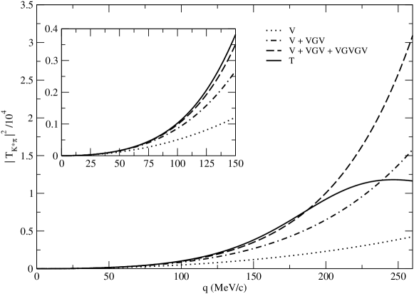
Figure 2: Comparison of the perturbative expansion to the unitarized amplitude for $K^{*}\pi\to K^{*}\pi$ with only one channel ($K^{*}\pi$) and in the chiral limit ($m_{\pi}=0$). All the lines represent the modulus square. Dotted line: tree level potential $(-V)$; dashed-dotted line: expansion of $T$ at one loop, $(-V)+(-V)G(-V)$; dashed line: expansion of $T$ at two loops, $(-V)+(-V)G(-V)+(-V)G(-V)G(-V)$; solid line: unitarized amplitude, $T$.

First we show, in Fig. 2, results for the $K^{*}\pi\to K^{*}\pi$ amplitude using only one channel ($K^{*}\pi$) and in the chiral limit ($m_{\pi}=0$). In Fig. 2 we can see the modulus squared of the amplitudes calculated with the approximations $(-V)$, $(-V)+(-V)G(-V)$, $(-V)+(-V)G(-V)+(-V)G(-V)G(-V)$ and the unitary amplitude. We can see that for low momenta there is a nice convergence of the perturbative series to the unitary result up to about $150\textrm{ MeV}/c$. However, the unitary amplitude has a resonant structure with a peak around $250\textrm{ MeV}/c$ where the perturbative expansion is seen to fail drastically. Note that the lowest order $(-V)$ (in the chiral limit) is of order $q$, as can be seen from Eq. (1) or expanding Eq. (7).

The real case has finite pseudoscalar masses and coupled channels ($\phi K$, $\omega K$, $\rho K$, $K^{*}\eta$, $K^{*}\pi$) and one has different thresholds for different channels. This case is shown in Fig. 3.

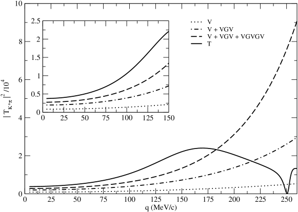
Figure 3: Same as Fig. 2 but with all the allowed $VP$ channels and with finite pseudoscalar masses

This fact changes the behavior of the amplitudes close to the $K^{*}\pi$ threshold, where they no longer vanish, and, although the perturbative expansion is seen to converge to the unitary amplitude, the convergence is now slower. Once more we see a lack of convergence when we get close to the resonance peak around $170\textrm{ MeV}/c$.

In Fig. 4 we show the same amplitudes as before for the $\omega\pi\to\omega\pi$ cases.

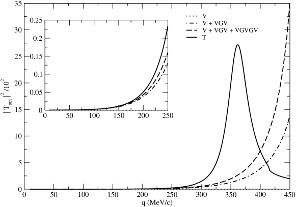
Figure 4: Same as Fig. 3 for the $\omega\pi\to\omega\pi$ case

Now, the tree level amplitude is zero, see Table 4, and the first resonance appears around $350\textrm{ MeV}/c$. We see that the convergence of the perturbative expansion extends up to higher momenta than in the previous case, up to about $250\textrm{ MeV}/c$. A combined conclusion from these two cases is that the perturbative expansion works well as far as we are not close to the lowest resonance, and of course, as far as $q$ is small compared to $\Lambda_{\chi}$. This reflects the mathematical theorem of complex variable that a series converges up to the first singularity, in our case the poles in the complex plane associated to the resonances. It is worth noting that what limits the convergence of the series expansion is the appearance of the lowest resonance, which in the present work appears at momenta much smaller than $\Lambda_{\chi}$. The unitary amplitude has no problems of convergence, based as it is in the $N/D$ method, as far as one used a proper interaction and included all relevant coupled channels. Up to energies of $\sqrt{s}\simeq 1.5\textrm{ GeV}$ we consider that we are taking into account the relevant channels. This is about a momentum of about $500\textrm{ MeV}/c$ for th $\rho\pi$ channel, which has the highest momentum. This momentum is still smaller than the $600\textrm{ MeV}/c$ of the $\pi\pi$ interaction, where the chiral unitary approach was shown to be rather successful in [10]. Nevertheless we shall comment in the results sections on possible consequences from the inclusion of channels other than $VP$.

Contrary to the perturbative expansion, the unitary amplitude allows for poles corresponding to bound states or resonances. In the next section we address this issue.

3 Search for poles

3.1 Unphysical Riemann sheets

The association of physical resonances to poles of the scattering matrix in unphysical Riemann sheets is a very powerful tool to identify the resonances. The results of the scattering theory say that bound states reflect as a pole for $\textrm{Im}(q)>0$ and $\textrm{Re}(q)=0$, with $q$ the momentum $q_{l}$ of Eq. (15), i.e., in the real $s$ axis below the lowest threshold. The resonances can appear only for $\textrm{Im}(q)<0$ which means $s$ with an argument larger than $2\pi$ and $\textrm{Re}(s)$ above the lowest threshold. This is what we will call second Riemann sheet (R2) for the function $T$ for the variable $s$. If these poles are not very far from the real axis they occur in $\sqrt{s}=(M\pm i\Gamma/2)\equiv\sqrt{s_{p}}$ with $M$ and $\Gamma$ the mass and width of the resonance respectively. Of course the only meaningful physical quantity is the value of the amplitudes for real $\sqrt{s}$, i.e., the reflexion of the pole on the real axis. Therefore, only poles not very far from the real axis would be easily identified experimentally as a resonance.

The effect of passing $s$ to R2 has consequences only for the $G$ functions. To evaluate $G$ in R2 we can use the Schwartz reflexion theorem which states that if a function $f(z)$ is analytic in a region of the complex plane including a portion of the real axis in which $f$ is real, then $[f(z^{*})]^{*}=f(z)$. The loop function $G_{l}$ satisfies these conditions, therefore, for $\textrm{Re}(\sqrt{s})>m_{l}+M_{l}$ we have

$$G_{l}(\sqrt{s}-i\epsilon)=[G_{l}(\sqrt{s}+i\epsilon)]^{*}=G_{l}(\sqrt{s}+i\epsilon)-i2\textrm{Im}G_{l}(\sqrt{s}+i\epsilon).$$ (16)

Since the beginning of R2 is equal to the end of R1 we have

$$G_{l}^{II}(\sqrt{s}+i\epsilon)=G_{l}^{I}(\sqrt{s}-i\epsilon)=G_{l}^{I}(\sqrt{s}+i\epsilon)-i2\textrm{Im}G_{l}^{I}(\sqrt{s}+i\epsilon).$$ (17)

where the superindices $I$ and $II$ refer to R1 and R2 respectively.

The imaginary part of the loop function can be very easily evaluated from Eq. (13), for instance with Cutkosky rules, giving $\textrm{Im}G_{l}^{I}(\sqrt{s}+i\epsilon)=-\frac{q}{8\pi\sqrt{s}}$.

In principle Eqs. (16) and (17) are true only very close to the real axis but, since the analytic continuation to general complex plane is unique we can write for a general $\sqrt{s}$

$$G_{l}^{II}(\sqrt{s})=G_{l}^{I}(\sqrt{s})+i\frac{q}{4\pi\sqrt{s}},$$ (18)

with $\textrm{Im}(q)>0$. In Eq. (18) one can use for $G_{l}^{I}$ either Eq. (2.2) or the result of the cutoff method.

One could also have gone to R2 by using Eq. (2.2) but with the solution of $q_{l}$ with $\textrm{Im}(q_{l})<0$, but again one finds the problem of the multivaluedness of the $\ln$ functions. We have checked, by comparing with the result obtained from Eq. (18), that one can use Eq. (2.2) as it is written with the prescription of the $\ln$ explained below Eq. (2.2) and using $\sqrt{s}$ in the form $a+ib$, $a$ and $b$ real.

When looking for poles we will use $G_{l}^{I}(\sqrt{s})$ for $\textrm{Re}(\sqrt{s})<m_{l}+M_{l}$ and $G_{l}^{II}(\sqrt{s})$ for $\textrm{Re}(\sqrt{s})>m_{l}+M_{l}$. This prescription gives the pole positions and half widths closer to those of the corresponding Breit-Wigner forms in the real axis. In this way, when being below the lowest threshold, we could also obtain possible pure bound states.

3.2 SU(3) symmetry breaking scan

The use of physical vector and pseudoscalar masses, both in the potential $V_{ij}$ as in the loop functions, allows for SU(3) symmetry breaking. By following a similar procedure to Refs. [20, 17], we are going to look for poles starting from the exact $SU(3)$ limit and breaking $SU(3)$ symmetry gradually. This can be accomplished by starting using a unique vector meson mass, $M_{0}$, and pseudoscalar mass, $m_{0}$, (obtained as an average of the physical masses inside each $SU(3)$ multiplet) and changing the masses in the following way:

$$M_{i}^{2}(x)=M_{0}^{2}+x(M_{i}^{2}-M_{0}^{2})$$

$$m_{i}^{2}(x)=m_{0}^{2}+x(m_{i}^{2}-m_{0}^{2}),$$ (19)

with $0\leq x\leq 1$. In this way, the masses used are the $SU(3)$ averaged masses for $x=0$ and the physical masses for $x=1$. In Fig. 5 we show the position of the poles for the $(S,I)$ channels $(0,0)$, $(0,1)$ and $(1,1/2)$, (the only $(S,I)$ channels for which we find poles), evaluating the loop functions with the subtraction constant method.

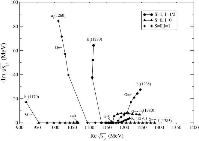
Figure 5: Trajectories of the poles in the scattering amplitudes obtained by increasing the $SU(3)$ breaking parameter, $x$, from $0$ to $1$. The loop functions are regularized by means of the subtraction constant method.

In the exact $SU(3)$ limit ($x=0$) we find two degenerate octet poles in all the $(S,I)$ channels at $\sqrt{s}=(1168+i0)\textrm{ MeV}$, and also a singlet pole for the $(0,0)$ channel at $\sqrt{s}=(1067+i0)\textrm{ MeV}$. Hence, our guess at the end of subsection 2.1 that there could be two octets and one singlet of dynamically generated resonances gets confirmed. As we break $SU(3)$ gradually, by increasing $x$, two branches for each $(S,I)$ channels of the octet and one for the singlet emerge. The branches end in the physical mass situation, $x=1$. Note that each branch for the $(0,0)$ and $(0,1)$ channels has well defined $G-$parity while this is not the case for $(1,1/2)$ since this corresponds to non-zero strangeness. In the plot we have also written for each pole our guess for the correspondence with physical $1^{+}$ resonances of the PDG. These assignments will be justified in the detailed discussion of section 4.

The plot in Fig. 5 is instructive but must be interpreted with caution. In principle, the real part of the pole position at $x=1$ should reflect the mass of the resonance while two times the imaginary part should be the width. One may wonder how stable are the results with respect to reasonable changes in the regularization scheme. An estimation of the uncertainties can be done by using the regularization method of fixing $G=0$ at the vector mass [22]. The results are qualitatively similar for the trajectories and the real part for the pole positions at $x=1$ differ in the worst of the cases in less than $100\textrm{ MeV}$ and in most cases by less than $30\textrm{ MeV}$. The imaginary part of the pole positions also differ in similar amounts, but relative to the absolute values of the mass and width of the resonances, the differences in the width are more significant. Yet, here we must observe that the width obtained so far is only a first approximation for the following reasons:

a) We have not considered other decay channels which are not made of a vector and a pseudoscalar. Other channels to which the resonance couples weakly can in practice give a sizeable partial decay width because of the large phase space available. For example, this would be the case of the $b_{1}(1235)$ going to four pions, where the phase space is favored with respect to our $VP$ channels. While including these extra channels in the coupled channels approach goes beyond the scope of the present work, it is important to note that the weaker strength of the couplings to these channels makes their repercussion on the real part of the pole positions less relevant since there are no restrictions of phase space for the real part of the amplitudes. Hence, we might expect small changes in he real part of the pole positions from these neglected sources, however, not altering the important fact that these poles appear for these quantum numbers.

b) The second reason is that so far we have not considered the width of the vector mesons in their propagators in the loop functions. For the case of the $\rho$ and the $K^{*}$ it is important to take this into consideration. We shall take this into account in the results section and we shall see that this modifies the width of the resonances but only very slightly their mass. We will also use another method to account for the width of the vector mesons by using the coupling of the resonances to the $VP$ channels and evaluating the partial decay widths by means of a convolution with the mass distribution of the vector and axial-vector mesons. This will be seen in the next chapter.

3.3 Couplings and partial decay widths

The physical interpretation of the poles comes clearer if we realize that close to a pole, and if it is not very close to a threshold, the amplitude takes the form of a Breit-Wigner structure. By looking at the structure of the covariant amplitude in the Appendix II Eq. (42) and the fact that the poles appear in the $Vb(1-b)$ term, close to a pole the amplitude has the form (in one channel for simplicity)

$$T\simeq\frac{Vb}{1-b}\left(g^{\mu\nu}-\frac{P^{\mu}P^{\nu}}{P^{2}}\right)\epsilon_{\mu}\epsilon^{\prime}_{\nu},$$ (20)

which has the structure of a resonant pole amplitude (see Fig. 6)

$$T\simeq g^{2}\frac{1}{P^{2}-M_{R}^{2}}\left(-g^{\mu\nu}+\frac{P^{\mu}P^{\nu}}{M_{R}^{2}}\right)\epsilon_{\mu}\epsilon^{\prime}_{\nu}.$$ (21)

Figure 6: Effective interpretation of the $PV\to PV$ scattering process close to a pole.

Generalizing to different channels and considering only the transverse polarizations, the amplitudes close to a pole in the second Riemann sheet can be expressed as

$$T_{ij}\simeq\frac{g_{i}g_{j}}{s-s_{p}},$$ (22)

where we have omitted the trivial $\vec{\epsilon}\cdot\vec{\epsilon}\,^{\prime}$ factor. Hence the factors $g_{i}$, which stand as the effective coupling of the dynamically generated axial-vector resonances to the channel $i$, can be calculated from the residues of the amplitudes at the complex poles.

With the values of the couplings we can evaluate the partial decay widths of the axial-vector mesons into each $VP$ channels, which reads

$$\Gamma_{A\to VP}=\frac{|g_{VP}|^{2}}{8\pi M_{A}^{2}}q.$$ (23)

In the case where there is little phase space for the decay or it takes place due to the width of the particles, we fold the expression for the width with the mass distribution of the particles as

$$\Gamma_{A\to VP} = \frac{1}{\pi^{2}}\int_{(M_{A}-2\Gamma_{A})^{2}}^{(M_{A}+2\Gamma_{A})^{2}}ds_{A}\int_{(M_{V}-2\Gamma_{V})^{2}}^{(M_{V}+2\Gamma_{V})^{2}}ds_{V}\,\,\Gamma_{AVP}(\sqrt{s_{A}},\sqrt{s_{V}})$$ (24)

$$\cdot Im\left\{\frac{1}{s_{A}-M_{A}^{2}+iM_{A}\Gamma_{A}}\right\}Im\left\{\frac{1}{s_{V}-M_{V}^{2}+iM_{V}\Gamma_{V}}\right\}$$

$$\cdot \Theta(\sqrt{s_{A}}-\sqrt{s_{V}}-M_{P})\Theta(\sqrt{s_{A}}-\sqrt{s_{A}^{th}})\Theta(\sqrt{s_{V}}-\sqrt{s_{V}^{th}}),$$

where $\Theta$ is the step function, $\Gamma_{AVP}=\frac{|g_{VP}|^{2}}{8\pi s_{A}}q$ with $q=\frac{1}{2\sqrt{s_{A}}}\lambda^{1/2}(s_{A},s_{V},M_{P}^{2})$, $\Gamma_{A}$ and $\Gamma_{V}$ are the axial and vector mesons total width and $\sqrt{s_{A}^{th}}$, $\sqrt{s_{V}^{th}}$, are the threshold energies for the dominant $A$ and $V$ decay channels.

In Eq. (24) the convolution is done using the masses and total widths of the particles taken from the PDG.

4 Detailed study of the $1^{+}$ resonances

4.1 $S=0$, $I=0$

In Fig. 7 we show the results for the diagonal $T_{ii}$ matrix elements as a function of the energy with the loop functions evaluated with the subtraction constant method (we will call it $a$ method) (left column), with the prescription of $G=0$ at the vector meson mass energy ($b$ method) (central column) and with the cutoff method including the widths of the vector mesons in the loops ($c$ method) (right column). This latter method evaluates Eq. (13) performing the $q^{0}$ integration analytically and the $\vec{q}$ integration with a cutoff $q_{max}=1000\textrm{ MeV}$ substituting $M_{l}^{2}\to M_{l}^{2}-iM_{l}\Gamma$.

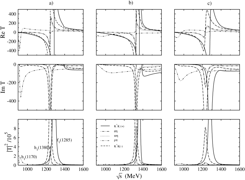
Figure 7: Amplitude for $S=0$, $I=0$, for the different allowed channels. Left column: subtraction constant method in the loop functions; central column: with the prescription of $G=0$ at the vector meson mass energy; right column: cutoff method considering vector meson width in the propagator.

We do not show the results with the cutoff method without widths in the vector meson propagator in the loops since they are very similar to the ones with the $a$ method (actually, the subtraction constant has been chosen to agree with the cutoff method). We can clearly see the reflexion on the real axis of the poles found in Fig. 5 in this $(0,0)$ channel, which corresponds to the $a$ method. The $a$ and $b$ methods give qualitative similar results but there are significant differences at low energies although not so large at higher energies. When we include the width in the vector meson propagators of the loops, we obtain a broadening of the amplitudes. All these discrepancies give an idea of the uncertainty we have in the model.

In Table 5 we show the position of the poles obtained with the $a$ method and the couplings to the different isospin channels.

$\sqrt{s_{p}}$	$919-i17$		$1245-i7$		$1288-i0$
	$g_{i}$	$|g_{i}|$	$g_{i}$	$|g_{i}|$	$g_{i}$	$|g_{i}|$
$\frac{1}{\sqrt{2}}(\bar{K}^{*}K+K^{*}\bar{K})$	$-$	$-$	$-$	$-$	$7230+i0$	$7230$
$\phi\eta$	$46-i13$	$48$	$-3311+i47$	$3311$	$-$	$-$
$\omega\eta$	$23-i28$	$36$	$3020-i22$	$3020$	$-$	$-$
$\rho\pi$	$-3453+i1681$	$3840$	$648-i959$	$1157$	$-$	$-$
$\frac{1}{\sqrt{2}}(\bar{K}^{*}K-K^{*}\bar{K})$	$781-i498$	$926$	$6147+i183$	$6150$	$-$	$-$

Table 5: Pole positions and couplings for $S=0$, $I=0$. (All the units are MeV.)

The pole at $919-i17\textrm{ MeV}$, which is found for the channels with negative $G-$parity, may be identified with the $h_{1}(1170)$ resonance. In the PDG the only decay channel seen so far is $\rho\pi$, although we find this pole in all the channels allowed by the quantum numbers, even if they are kinematically closed. However, in Fig. 7 these other channels are difficult to see since the amplitude is dominated in this region by the $\rho\pi$ channel.

The partial widths obtained for the axial-vector resonance decaying into $VP$ are presented in Table 6.

	$\Gamma_{tot}^{exp}$	$\Gamma_{i}^{exp}$	$\Gamma_{i}^{th}(a)$	$\Gamma_{i}^{th}(b)$
$h_{1}(1170)\to\bar{K}^{*}K+c.c.$	$360\pm 40$	$-$	$0.5$	$1.4$
$h_{1}(1170)\to\rho\pi$	′′	$seen$	$77$	$115$
$h_{1}(1170)\to\omega\eta$	′′	$-$	$0$	$0$
$h_{1}(1170)\to\phi\eta$	′′	$-$	$0$	$0$
$h_{1}(1380)\to\bar{K}^{*}K+c.c.$	$91\pm 30$	$seen$	$45$	$36$
$h_{1}(1380)\to\rho\pi$	′′	$-$	$9$	$4$
$h_{1}(1380)\to\omega\eta$	′′	$-$	$25$	$16$
$h_{1}(1380)\to\phi\eta$	′′	$-$	$0$	$0$
$f_{1}(1285)\to\bar{K}^{*}K+c.c.$	$24\pm 1$	$not\,seen$	$0.3$	$0.2$

Table 6: Partial decay widths for $S=0$, $I=0$. (All the units are MeV.)

The results that we obtain are compatible with the scarce experimental information in the sense that the only decay channel seen is the $\rho\pi$, which is the only relevant in our case. We can see that the widths for this channel calculated with the $a$ and $b$ methods are qualitatively similar. It is also instructive to see that with the $c$ method (see 3rd column of Fig. 7) we see the apparent full width of the resonance (around $90\textrm{ MeV}$), which is in reasonable agreement with the sum of all the partial decay widths in Table 6 for the $h_{1}(1170)$.

The $1245-i7\textrm{ MeV}$ pole can be assigned to the $h_{1}(1380)$ resonance. Note that in the PDG the isospin of this resonance is not given, although in the classification schemes it is assumed to have $I=0$. Our assignment, as well as suggested in [22], is also $I=0$.

The only experimentally observed decay channel of the $h_{1}(1380)$ is $\bar{K}^{*}K$ (with $G-$parity negative). In Table 6 we see our results for the different partial decay widths. It is difficult to extract conclusions from Table 6 given the scarce experimental data, but we should stress that the only channel experimentally seen is precisely the dominant one in our calculations. In this case the sum of our partial $VP$ decay channels is compatible with the total experimental width. We also see that method $c$ gives a width (around $40\textrm{ MeV}$) qualitatively similar to the sum of the partial decay widths in Table 6.

The pole at $1288-i0\textrm{ MeV}$ is below the $\bar{K}^{*}K$ threshold which is the only allowed $PV$ channel for positive $G-$parity, and therefore the pole appears as a bound state of $\bar{K}^{*}K+c.c.$. Actually, in Fig. 7 with the $a$ and $b$ methods $|T|^{2}$ goes to infinity at the pole position. It is reasonable to assign this pole to the $f_{1}(1285)$ resonance. The reason why we do not get width for this resonance, while in the PDG it is said to be $24\textrm{ MeV}$, is because there are other decay channels different to $VP$ that we are not obviously considering, (like $4\pi$ ($33$%), $\eta\pi\pi$ ($52$%) or $K\bar{K}\pi$ ($10$%)) . In fact the $\bar{K}^{*}K+c.c.$ is quoted in the PDG as ”not seen” which agrees, in a first approximation, with the result obtained here as a bound state. If we evaluate the partial decay width into this channel, with the coupling obtained and with the convolution of the widths we get about $0.3\textrm{ MeV}$ which justifies why this decay channel has so far not been seen. This small number is actually rather unstable since it can be made even an order of magnitude bigger by enlarging the limits in the convolution of Eq. (24). The apparent width from the $|T|^{2}$ plot when considering the vector meson width in the propagator of the loop functions is around $20\textrm{ MeV}$. With all these apparent instabilities in the widths, one should not lose the important point which is that, comparatively to the other resonances, the width for this resonance is very small. It is worth noting that the $f_{1}(1285)$ couples only to $K^{*}\bar{K}$ in our theory and with such a large strength qualifies strongly as a quasibound $K^{*}\bar{K}$ or $\bar{K}^{*}K$ state. The small experimental total width indicates a small coupling to other channels which are kinematically open and barely change the nature of the resonance as a bound system of $K^{*}\bar{K}$.

When arriving to this point it is important to note that there is experimentally another resonance, the $f_{1}(1420)$, which is assigned by the PDG to the $1^{++}$ nonet. However, in our scheme this resonance has no counterpart. This is because, as explained in subsections 2.1 and 3.2, the interaction of two octets give one singlet plus two octets (three poles), therefore there is no way, with the interaction of one vector and one pseudoscalar mesons, to generate dynamically one more pole in this channel and, therefore, there is no room for one more resonance like the $f_{1}(1420)$. Therefore, in our scheme, the $f_{1}(1420)$ cannot be considered as a dynamically generated resonance from the $PV$ interaction.

On the other hand, the $h_{1}(1170)$ state that we generate (the original singlet in Fig. 5) has the same quantum numbers as the isoscalar member of the octet of the $b_{1}(1235)$, the $h_{1}(1380)$, and hence the set of the $b_{1}(1235)$, $h_{1}(1170)$ and $h_{1}(1380)$, together with the strange partners that we will discuss below, agree with the association of a nonet to all these states of the PDG.

4.2 $S=0$, $I=1$

In Fig. 8 we show the results for the $|T|^{2}$ with the same three methods used in the previous subsection.

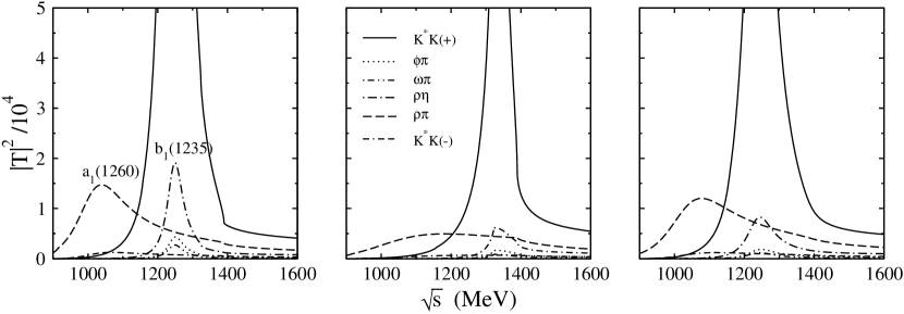
Figure 8: Amplitude for $S=0$, $I=1$, for the different channels. Left plot: subtraction constant method in the loop functions; central plot: with the prescription of $G=0$ at the vector meson mass energy; right plot: cutoff method considering vector meson width in the propagator.

We clearly see the reflexions in the real axis of the poles found in the complex plane, (shown in Table 7).

$\sqrt{s_{p}}$	$1011-i84$		$1247-i28$
	$g_{i}$	$|g_{i}|$	$g_{i}$	$|g_{i}|$
$\frac{1}{\sqrt{2}}(\bar{K}^{*}K+K^{*}\bar{K})$	$-$	$-$	$6172-i75$	$6172$
$\phi\pi$	$-$	$-$	$2087-i385$	$2122$
$\omega\pi$	$-$	$-$	$-1869+i300$	$1893$
$\rho\eta$	$-$	$-$	$-3041+i498$	$3082$
$\rho\pi$	$-3795+i2330$	$4453$	$-$	$-$
$\frac{1}{\sqrt{2}}(\bar{K}^{*}K-K^{*}\bar{K})$	$1872-i1486$	$2390$	$-$	$-$

Table 7: Pole positions and couplings for $S=0$, $I=1$.

The pole at $1247-i28\textrm{ MeV}$, which is found for the channels with positive $G-$parity, may be assigned to the $b_{1}(1235)$ resonance. In the PDG the full width is quoted to be $142\textrm{ MeV}$ and the decay channels are quoted as $\omega\pi$ (dominant), $\rho\eta$ (seen), $4\pi$ ($<50$%), $K\bar{K}\pi$ ($<14$%) and $\phi\pi$ ($<1.5$%), (See Table 8).

	$\Gamma_{tot}^{exp}$	$\Gamma_{i}^{exp}$	$\Gamma_{i}^{th}(a)$	$\Gamma_{i}^{th}(a)$
$b_{1}(1235)\to\bar{K}^{*}K+c.c.$	$142\pm 9$	$-$	$7$	$10$
$b_{1}(1235)\to\phi\pi$	′′	$<1.5$%	$12$	$13$
$b_{1}(1235)\to\omega\pi$	′′	$dominant$	$25$	$25$
$b_{1}(1235)\to\rho\eta$	′′	$seen$	$8$	$9$
$a_{1}(1260)\to\rho\pi$	$250-600$	$seen(60$%$?)$	$106$	$156$
$a_{1}(1260)\to\bar{K}^{*}K+c.c.$	′′	$seen(<10$%$?)$	$6$	$11$

Table 8: Partial decay widths for $S=0$, $I=1$. (All the units are MeV.)

Therefore one could expect that the $VP$ decay channels would account for around $50$% of the total width. This is compatible with what we obtain, as can be seen in Table 8. Note also that the channel quoted as dominant in the PDG is indeed the dominant one in our results. It is also interesting to call the attention to the fact that the strongest coupling of the $b_{1}(1235)$ is to $K^{*}\bar{K}$ as it was the case of the $h_{1}(1380)$, consistently with the fact that they belong to the same $SU(3)$ octet in the $SU(3)$ limit. It is interesting to see that this feature remains in spite of the $SU(3)$ breaking. The method $c$ provides an apparent total width of about $80\textrm{ MeV}$.

The pole at $1011-i84\textrm{ MeV}$, which is found for the channels with negative $G-$parity, could be assigned to the $a_{1}(1260)$ resonance. Note that the values for the mass and width quoted for this resonance in the PDG, $1230\pm 40$ and $250-600\textrm{ MeV}$ respectively, have a large uncertainty. This can justify the discrepancy in the position of the pole we obtain. For the partial decays widths there is no good data quoted in the PDG (every one of the many decay channels are just quoted as ”seen”). However, in the detailed explanation in the PDG, some experiment gives for $\rho\pi$ $60$% and for $\bar{K}^{*}K+c.c.$ $8-15\textrm{ MeV}$%, what would be in reasonable agreement with what we obtain. The method $c$ provides an apparent width of about $300\textrm{ MeV}$ which is tied to he slow fall down of $|T|^{2}$ at the right of the peak, which differ from a typical Breit-Wigner shape.

It is interesting to note that the octet of the $a_{1}(1260)$ resonance has been considered as one of the fundamental fields in chiral theories which deal explicitly with spin-1 fields [25]. In this latter work the $L_{i}$ parameters of [28] have been derived assuming exchange of these vector mesons (and scalars). The comment is worth making because the use of the chiral interaction between the pseudoscalar and vector mesons used here, together with the unitarization procedure, generates dynamically the $a_{1}(1260)$ resonance and, hence, introducing it further as an explicit degree of freedom would lead to doublecounting.

There is another observation worth making which is the fact that there is another $a_{1}$ resonance in the PDG at higher energies, the $a_{1}(1640)$, which we do not generate dynamically and is more likely to be a genuine $q\bar{q}$ meson. At the same time there is another observation to make which is the fact that no other $b_{1}$ resonance is quoted in the PDG.

4.3 $S=1$, $I=1/2$

In Fig. 9 we show the results for the amplitudes with the same three methods considered in the other channels.

Figure 9: Amplitude for $S=1$, $I=1/2$, for the different channels. Left plot: subtraction constant method in the loop functions; central plot: with the prescription of $G=0$ at the vector meson mass energy; right plot: cutoff method considering vector meson width in the propagator.

In Table 9 we show the pole positions and the couplings obtained.

$\sqrt{s_{p}}$	$1112-i64$		$1216-i4$
	$g_{i}$	$|g_{i}|$	$g_{i}$	$|g_{i}|$
$\phi K$	$1587-i872$	$1811$	$1097-i400$	$1168$
$\omega K$	$-1860+i649$	$1970$	$-1033+i375$	$1099$
$\rho K$	$-1524+i1154$	$1912$	$5274+i297$	$5282$
$K^{*}\eta$	$27+i155$	$157$	$3459-i95$	$3460$
$K^{*}\pi$	$4187-i2098$	$4683$	$340-i984$	$1041$

Table 9: Pole positions and couplings for $S=1$, $I=1/2$.

The lowest pole couples strongly to $K^{*}\pi$, very weakly to $K^{*}\eta$ and moderately to the rest of channels. On the contrary, the higher pole couples strongly to $\rho K$ and $K^{*}\eta$ while moderately to the other channels.

In Fig. 10 we plot, as an illustrative example, the modulus squared of the scattering matrix in the second Riemann sheet for three different channels. The pole structure can be clearly seen as well as the relative strength of each channel in the two different poles (similar plots can be obtained for the rest of channels).

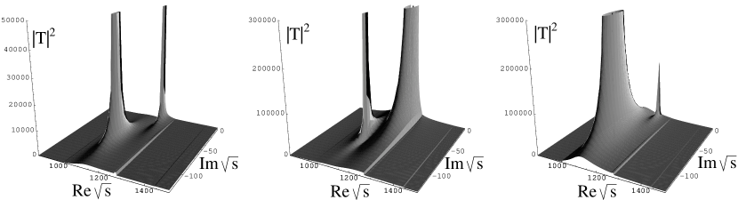
Figure 10: $|T|^{2}$ in the second Riemann sheet for $\phi K$, $\rho K$ and $K^{*}\pi$ channels for $S=1$, $I=1/2$.

In the PDG there are two physical $S=1$, $I=1/2$, resonances with $J^{P}=1^{+}$, which are the $K_{1}(1270)$ and the $K_{1}(1400)$. Actually these two resonances have been usually considered to be a mixture of the $K_{1}$ members of the $1^{++}$ and $1^{+-}$ octets, called $K_{1A}$ and $K_{1B}$ respectively. At this point we have difficulty assigning the poles found to these resonances. In order to have a feeling of which reasonable assignment to make we study the partial decay widths of these two resonances. This is shown in Table 10. In the table we have assumed for convolution purposes and phase space the mass of the resonance to be $1270\textrm{ MeV}$ and in the last column we show the expected partial decay width coming from the poles in Table 9. We can see that the resonance at $1112\textrm{ MeV}$ couples strongly to the $K^{*}\pi$ and leads to a partial decay width in this channel of $113\textrm{ MeV}$ (around $150\textrm{ MeV}$ should we considered the mass to be $1400\textrm{ MeV}$). On the other hand, the $1216\textrm{ MeV}$ resonance couples dominantly to $\rho K$. In view of this, one would be tempted to assign the $1112\textrm{ MeV}$ pole to the $K_{1}(1400)$ resonance and the $1216\textrm{ MeV}$ pole to the $K_{1}(1270)$ since this is the experimental case. Yet, the difference of $300\textrm{ MeV}$ in the mass in the case of the $K_{1}(1400)$ is not an appealing feature, since this difference is much larger than the $K_{1}(1400)$ width ($174\textrm{ MeV}$). There is another possible scenario which we find more appealing. The detailed explanation of the PDG on the determination of the decay widths shows a clear discrepancy between different methods of determination of the $K_{1}(1270)$ width. In particular, a set of experiments using $K$ beams leads to much larger widths (about a factor three) than another set that uses pion beams. This could find an explanation if one assumed that the experimental $K_{1}(1270)$ resonance is a superposition of two resonances that couple with different strength to a particular channel. This is indeed the case for the two poles that we find, one of them coupling strongly to $K^{*}\pi$ and the other one to $\rho K$. Different experiments which favor mechanisms that give a bigger weight to one of these channels would lead to very different widths of the resonance. This is the case with the recent findings that the $\Lambda(1405)$ resonance corresponds to actually two poles and different experiments favor one or the other pole, leading to different visible widths of the resonance [17, 18, 29].

There are some experimental features in the different experiments that could be understood within the two pole structure that we obtain. Indeed, some experiments provide a dominance of the $K_{1}(1270)$ decay into $\rho K$ [30, 31, 32] while other experiments show a clear dominance of the $K^{*}\pi$ decay mode [33]. In our theoretical approach the dominance of the $\rho K$ decay in a reaction has to be interpreted as a sign that the dynamics of the reaction favours the second pole (which couples mostly to $\rho K$) and this would have a small width. This is indeed the case experimentally, and the total width is about $60\textrm{ MeV}$ (similar to our results). On the other hand, the dominance of the $K^{*}\pi$ decay channel in another experiment would have to be interpreted as the dynamics of this reaction favouring the coupling to the first resonance. In this case the total width would be large and indeed this is what is seen in the experiment of [33] where the total width is about $190\textrm{ MeV}$ (we obtain $125\textrm{ MeV}$ with the $a$ method or $200\textrm{ MeV}$ with the $b$ method).

In Ref. [22] a broad bump in the speed plot was associated to the $K_{1}(1400)$ resonance but we find no pole in that amplitude in that region.

	$\Gamma_{tot}^{exp}$	$\Gamma_{i}^{exp}$	$\Gamma_{i}^{th}(a)$	$\Gamma_{i}^{th}(b)$
$K_{1}(1270)\to\phi K$	$90\pm 20$	$-$	$(0,0)$	$(0,0)$
$K_{1}(1270)\to\omega K$	′′	$11$%	$(5,2)$	$(10,0.1)$
$K_{1}(1270)\to\rho K$	′′	$42$%	$(7,52)$	$(5,12)$
$K_{1}(1270)\to K^{*}\eta$	′′	$-$	$(0,0)$	$(0,0)$
$K_{1}(1270)\to K^{*}\pi$	′′	$16$%	$(113,6)$	$(194,1)$

Table 10: Partial decay widths for $S=1$, $I=1/2$. In the last column, the first element is the value obtained with the coupling to the lower pole and the second element is the result with the coupling to the higher pole. (All the units are MeV.)

It is interesting to see that, when breaking the $SU(3)$ symmetry, the $S=0$ states of the two octets in Fig. 5 do not mix because they have well defined $G-$parity (this is opposite to the case of the meson baryon interaction [17] where one did not have this constraint). However, when we go to $S\neq 0$, then the states are no longer eigenstates of $G-$parity and the octets mix. This is a well known case for the $K_{1}$ axial-vectors where there is much discussion about the mixing in the literature.

We next proceed to see which is the mixing angle for the two poles in $S=1$, $I=1/2$, that we find. We write

$$|K_{1}(1270),1> = \sin\theta|K_{1A}>+\cos\theta|K_{1B}>,$$

$$|K_{1}(1270),2> = \cos\theta|K_{1A}>-\sin\theta|K_{1B}>,$$ (25)

where $|K_{1}(1270),1>$ is the state associated to the lower mass pole and $|K_{1}(1270),2>$ to the upper mass pole. In Eq. (25) $|K_{1A}>$ corresponds to the $SU(3)$ $|8_{a},1,1/2,+1/2>$ state and $|K_{1B}>$ to the $|8_{s},1,1/2,+1/2>$ state, (in the notation $|irrep,Y,I,I_{3}>$, with $irrep$ being the name of the irreducible representation of $SU(3)$, $Y$ the hypercharge, $I$ the total isospin and $I_{3}$ the third component of $I$). (Note that we have chosen $I_{3}=+1/2$ although the following discussion works obviously for any allowed $I_{3}$).

Figure 11: Schematic interpretation of the coupling of the dynamically generated axial-vector resonance to a $PV$ state.

The couplings considered so far are (see Fig. 11), by definition,

$$g_{i}\equiv<R|t|i(I=1/2,I_{3}=+1/2)>,$$ (26)

where $|R>$ is the generic name for the physical resonance associated to either pole. By making use of $SU(3)$ Clebsch-Gordan coefficients, we can obtain the relation of the couplings in isospin base to the ones in $SU(3)$ base, giving

$$\left(\begin{array}[]{c}\vspace{0.13cm}g_{\phi K}\\ \vspace{0.13cm}g_{\rho K}\\ \vspace{0.13cm}g_{K^{*}\eta}\\ \vspace{0.13cm}g_{K^{*}\pi}\\ \end{array}\right)=\left(\begin{array}[]{cccc}\vspace{0.1cm}-\sqrt{\frac{3}{10}}&\frac{1}{\sqrt{6}}&\frac{1}{\sqrt{30}}&\frac{1}{\sqrt{6}}\\ \vspace{0.1cm}-\frac{1}{2\sqrt{5}}&-\frac{1}{2}&-\frac{3}{2\sqrt{5}}&\frac{1}{2}\\ \vspace{0.1cm}\frac{3}{2\sqrt{5}}&\frac{1}{2}&-\frac{1}{2\sqrt{5}}&\frac{1}{2}\\ \vspace{0.1cm}\frac{1}{2\sqrt{5}}&-\frac{1}{2}&\frac{3}{2\sqrt{5}}&\frac{1}{2}\\ \end{array}\right)\cdot\left(\begin{array}[]{c}\vspace{0.13cm}g_{27}\\ \vspace{0.13cm}g_{\bar{10}}\\ \vspace{0.13cm}g_{8_{s}}\\ \vspace{0.13cm}g_{8_{a}}\\ \end{array}\right)$$ (27)

By using in the left hand side of Eq. (27) the values obtained in Table 9 we get the results shown in Table 11.

	$1112-i64$	$1216-i4$
$g_{27}$	$-8+i94$	$316-i21$
$g_{\bar{10}}$	$-346+i15$	$-406+i51$
$g_{8_{s}}$	$4259-i2455$	$-3783-i947$
$g_{8_{a}}$	$2317-i928$	$5208-i636$

Table 11: Couplings for $S=1$, $I=1/2$, in SU(3) base.

As mentioned after Eq. (10), the singlet component of the $\phi$ and $\omega$ (see Eq. (8)) does not lead to an interaction term, and this is already assumed in Eq. (27) where only the octet component of the $\phi$ is taken. We could as well have taken instead of $g_{\phi K}$ in Eq. (27) the coupling $-\sqrt{2}g_{\omega K}$ and in the exact $SU(3)$ limit this would lead to the same results. When $SU(3)$ is broken, the use of either coupling in the Eqs. (27) will give us an idea about the uncertainties in this $SU(3)$ decomposition.

In Table 11 we can see that the couplings to the $27-$plet and the decuplet are almost negligible in comparison to the two octets, in fact, they are compatible with zero within the uncertainties we can assume in our model. This means that the two poles found are essentially a mixing of the antisymmetric and symmetric octets. The above reasoning is more than qualitative since it allows us to quantify the weight of the $SU(3)$ components of the resonance and therefore the mixing angle defined in Eq. (25). In order to obtain this mixing angle let us write Eq. (25) in a more generic way:

$$|R>=a_{27}|27,R>+a_{\bar{10}}|\bar{10},R>+a_{8_{s}}|8_{s},R>+a_{8_{a}}|8_{a},R>$$ (28)

where we have used the short notation $|27,R>\equiv|27,1,1/2,+1/2,R>$ and so on for the rest. The $a_{j}$ coefficients must satisfy $\sum|a_{j}|^{2}=1$. To obtain the mixing angle $\theta$ we have to evaluate $a_{8_{s}}$ and $a_{8_{a}}$ since, by definition, they are $a_{8_{s}}=\cos\theta$ and $a_{8_{a}}=\sin\theta$ for $|K_{1}(1270),1>$.

On the other hand, up to lowest order in $SU(3)$ breaking, we have

$$g_{8_{s}} \equiv <R|t|8_{s}>\simeq a^{*}_{8_{s}}<8_{s},R|t|8_{s}>\equiv a^{*}_{8_{s}}t_{8_{s}}\qquad a),$$

$$g_{8_{a}} \equiv <R|t|8_{a}>\simeq a^{*}_{8_{a}}<8_{a},R|t|8_{a}>\equiv a^{*}_{8_{a}}t_{8_{a}}\qquad b).$$ (29)

Therefore, had we know $t_{8_{s}}$, $t_{8_{a}}$, we would know $a_{8_{s}}$, $a_{8_{a}}$, by using $g_{8_{s}}$, $g_{8_{a}}$, from Table 11. To evaluate $t_{8_{s}}$ and $t_{8_{a}}$ we can go to the $SU(3)$ limit, which by virtue of Eq. (11) should be the same. In this limit the two octet poles are in the same place. The couplings $t_{8_{s}}$, $t_{8_{a}}$, are easily evaluated since the matrix elements of the potential in the $SU(3)$ base are already known in Eq. (11). Hence, by performing the Bethe-Salpeter resummation in this base, we readily obtain the poles corresponding to each $SU(3)$ irreducible representations and the couplings. The amplitudes behave in the pole as

$$<8_{s}|T|8_{s}>=\frac{t_{8_{s}}^{2}}{s-s_{p}},$$ (30)

and analogously for $8_{a}$ and singlet, the only channels where there are poles. We find $t_{8_{s}}=t_{8_{a}}=5568\textrm{ MeV}$.

In the case of physical masses, $x=1$, using the same values for $t_{8_{s}}$ and $t_{8_{a}}$ that we have obtained in the $SU(3)$ limit and the couplings $g_{8_{s}}$, $g_{8_{a}}$, of Table 11, we obtain the following results: for the pole $1112-i64\textrm{ MeV}$ we get from Eq. (29a) $\theta\simeq 28^{o}$, and from Eq. (29b) $\theta\simeq 27^{o}$. Should we have used $-\sqrt{2}g_{\omega K}$ instead of $g_{\phi K}$ in the calculations we would get $\theta\simeq 22^{o}$ from Eq. (29a) and $\theta\simeq 34^{o}$ from Eq. (29b). These discrepancies give an idea of the uncertainties in our calculations.

For the pole $1216-i4\textrm{ MeV}$, we get from Eq. (29a) $44^{o}$, and from Eq. (29b) $20^{o}$. And with $g_{\omega K}$ $43^{o}$ and $11^{o}$ respectively, which implies that we have a larger uncertainty in this case. In fact, for the pole $1112-i64\textrm{ MeV}$ we get $\sum|a_{j}|^{2}=0.98$ by using $g_{\phi K}$ and $1.17$ by using $g_{\omega K}$, and for the pole $1216-i4\textrm{ MeV}$, $1.38$ and $1.43$. The deviation of these numbers with respect to $1$ gives an idea of the uncertainties.

I summary, we get a mixing angle of the order of $30^{o}$ with an uncertainty of about $40$%. We should however refrain from making any association of the mixing angle found here with the mixing angle of $K_{1A}$, $K_{1B}$, mentioned in the literature since this latter one is used to produce the $K_{1}(1270)$ and $K_{1}(1400)$ resonances and here we are mixing $K_{1A}$, $K_{1B}$, to produce $|K_{1}(1270),1>$ and $|K_{1}(1270),2>$.

Along this work we have devoted some attention to uncertainties in the theory. We would like to call the attention to another source of uncertainties which would affect all channels. So far we have used only the pion decay constant, $f=f_{\pi}=92\textrm{ MeV}$, in the Lagrangian. We could have used different values for $f_{\pi}$, $f_{K}$, $f_{\eta}$. In order to estimate uncertainties from this source we have proceeded as in [13] and taken an average $f=1.15f_{\pi}$. We find that all the poles obtained so far still appear but the pole positions are somewhat changed. The trajectories of the poles in the complex plane are essentially the same but with real parts shifted about $50\textrm{ MeV}$ to higher energies (using the same subtraction constant). The imaginary parts are accordingly increased since there is now more phase space. The most significant changes in the imaginary part of the pole positions are for the poles associated to the $h_{1}(1170)$ ($100$% increase), $a_{1}(1260)$ ($40$% increase) and $K_{1}(1270;1)$ ($50$% increase) and small changes in the rest. These increases are mostly tied to the increased phase space. However, we have so far evaluated the partial decay widths of the resonances, using the couplings obtained and the physical masses of the resonances. We have checked that the couplings of the resonances barely change with the use of the new $f$ constant (less than $10$% change in general and less than $5$% in the dominant channels) and hence, within the uncertainties discussed along the work, the results and the conclusions are unchanged from this new source of uncertainty.

The overall conclusion of all these tests is that the existence of the poles and their basic properties are very solid and not contingent to the difference sources of uncertainties discussed along the paper.

5 Conclusions

In this work we have done a systematic search for possible $J^{PC}=1^{++},1^{+-}$, dynamically generated resonances through the interaction of vector and pseudoscalar mesons. The starting point has been a chiral Lagrangian which, by expanding up to two pseudoscalar fields, leads to a Weinberg-Tomozawa term which accounts for the two-vectors and two-pseudoscalar meson interaction. From this Lagrangian we have argued, by going to the $SU(3)$ limit that from the interaction of the two octets we could expect attraction for one singlet and two octets. After that, we have implemented unitarity in coupled channels to account for the resummation of $VP$ loops in $L=0$. This resummation has been accounted for by means of a Bethe-Salpeter like equation in coupled channels, where some subtleties in the evaluation of the loop functions coming from the use of vector mesons have been discussed. The regularization of the loops has been done with dimensional regularization by means of a subtraction constant fixed to agree with the numerical result obtained performing the integration with a cutoff of natural size. We also compare our method with another one where the loop functions are fixed to zero when $\sqrt{s}$ is equal to the vector meson mass. This served to have an idea of uncertainties in the theory.

We have looked for poles of the scattering amplitudes in the second Riemann sheet. In the $SU(3)$ symmetric case, considered by taking equal masses for the vectors and equal masses for the pseudoscalars, we found two poles in the same position corresponding to two degenerate octets and one pole corresponding to the singlet. As $SU(3)$ symmetry is gradually broken, the two degenerate poles split apart in trajectories (different for each $(S,I)$ channel) ending in the physical situation, when the physical masses are used.

By evaluating the residues of the amplitudes in the poles, we have obtained the couplings of the axial-vector dynamically generated resonances to each $VP$ channel, which has allowed us to evaluate the different partial decay widths. In view of the information supplied by the pole positions, couplings and partial widths, we have done a correspondence of the poles found to the $h_{1}(1170)$, $h_{1}(1380)$, $f_{1}(1285)$, $b_{1}(1235)$, $a_{1}(1260)$ and $K_{1}(1270)$. For this latter case we found actually two poles coupled strongly to $K^{*}\pi$ and $K\rho$ respectively which also differed appreciably in the width. We suggested that different experiments give different weight to each of these resonances and this could explain the discrepancies in the widths obtained in different reactions. This would also explain the correlation found between experiments finding a dominance of the $\rho K$ decay (which produce a small width) and those finding a dominance of the $K^{*}\pi$ decay mode (which produce a large width). We also evaluated the couplings of our two $K_{1}(1270)$ states, finding a reasonable mixing of around $30^{o}$.

The only axial-vector resonances for which we do not find poles are the $f_{1}(1420)$ and the $K_{1}(1400)$ for different reasons: from the interaction of two octets one can only generate one singlet and two octets, therefore there is no room for more poles apart from those discussed above. Actually we only found a pole with the $f_{1}$ quantum numbers which suits better to the $f_{1}(1285)$. In the two poles that we find in the $S=1$, $I=1/2$, channel there are no clues to identify one of them to the $K_{1}(1400)$ resonance.

The conclusions reached in this paper about the dynamical nature of these axial-vector mesons should have experimental repercussions in the sense that, with the information obtained in the present work, one can make predictions for production of these resonances in different reactions, which are amenable of experimental search. This has been the case for other dynamically generated resonances and we hope the present paper encourages work in this direction.

References

- [1] S. Weinberg, PhysicaA 96 (1979) 327.
- [2] J. Gasser and H. Leutwyler, Nucl. Phys. B250 (1985) 465, 517, 539.
- [3] U. G. Meissner, Rep. Prog. Phys. 56 (1993) 903; V. Bernard, N. Kaiser and U. G. Meissner, Int. J. Mod. Phys. E4 (1995) 193.
- [4] G. Ecker, Prog. Part. Nucl. Phys. 35 (1995) 1.
- [5] A. Dobado and J. R. Pelaez, Phys. Rev. D 56 (1997) 3057.
- [6] N. Kaiser, P. B. Siegel and W. Weise, Phys. Lett. B 362 (1995) 23
- [7] N. Kaiser, T. Waas and W. Weise, Nucl. Phys. A 612 (1997) 297.
- [8] J. A. Oller and E. Oset, Nucl. Phys. A 620 (1997) 438 [Erratum-ibid. A 652 (1999) 407].
- [9] J. A. Oller, E. Oset and J. R. Pelaez, Phys. Rev. D 59 (1999) 074001 [Erratum-ibid. D 60 (1999) 099906].
- [10] J. A. Oller and E. Oset, Phys. Rev. D 60 (1999) 074023.
- [11] N. Kaiser, Eur. Phys. J. A 3 (1998) 307.
- [12] V. E. Markushin, Eur. Phys. J. A 8 (2000) 389.
- [13] E. Oset and A. Ramos, Nucl. Phys. A 635 (1998) 99.
- [14] J. C. Nacher, A. Parreno, E. Oset, A. Ramos, A. Hosaka and M. Oka, Nucl. Phys. A 678 (2000) 187.
- [15] J. A. Oller and U. G. Meissner, Phys. Lett. B 500 (2001) 263.
- [16] T. Inoue, E. Oset and M. J. Vicente Vacas, Phys. Rev. C 65 (2002) 035204.
- [17] D. Jido, J. A. Oller, E. Oset, A. Ramos and U. G. Meissner, Nucl. Phys. A 725 (2003) 181.
- [18] C. Garcia-Recio, M. F. M. Lutz and J. Nieves, Phys. Lett. B 582 (2004) 49.
- [19] E. E. Kolomeitsev and M. F. M. Lutz, Phys. Lett. B 585 (2004) 243.
- [20] S. Sarkar, E. Oset and M. J. Vicente Vacas, Nucl. Phys. A in print, arXiv:nucl-th/0407025.
- [21] J. R. Pelaez, Phys. Rev. Lett. 92 (2004) 102001.
- [22] M. F. M. Lutz and E. E. Kolomeitsev, Nucl. Phys. A 730 (2004) 392.
- [23] S. Eidelman et al. [Particle Data Group], Phys. Lett. B 592 (2004) 1.
- [24] M. C. Birse, Z. Phys. A 355 (1996) 231.
- [25] G. Ecker, J. Gasser, A. Pich and E. de Rafael, Nucl. Phys. B 321 (1989) 311.
- [26] S. Weinberg, Phys. Rev. Lett. 17 (1966) 616.
- [27] Y. Tomozawa, Nuovo Cim. 46A (1966) 707.
- [28] J. Gasser and H. Leutwyler, Annals Phys. 158 (1984) 142.
- [29] T. Hyodo, A. Hosaka, E. Oset, A. Ramos and M. J. Vicente Vacas, Phys. Rev. C 68 (2003) 065203.
- [30] P. Gavillet et al. [Amsterdam-CERN-Nijmegen-Oxford Collaboration], Phys. Lett. B 76 (1978) 517.
- [31] S. Rodeback et al. [CERN-College de France-Madrid-Stockholm Collaboration], Z. Phys. C 9 (1981) 9.
- [32] D. J. Crennell, H. A. Gordon, K. W. Lai and J. M. Scarr, Phys. Rev. D 6 (1972) 1220.
- [33] A. Firestone, G. Goldhaber, D. Lissauer and G. H. Trilling, Phys. Rev. D 5 (1972) 505.
- [34] L. Roca, J. E. Palomar and E. Oset, Phys. Rev. D 70 (2004) 094006.
- [35] D. Cabrera, E. Oset and M. J. Vicente Vacas, Nucl. Phys. A 705 (2002) 90.