CLNS 05/1913

FERMILAB-PUB-05-032-T

SLAC-PUB-11045

hep-ph/0503263
March 25, 2005

Factorization in $B\to V\gamma$ Decays

T. Becher^(a), R.J. Hill^(b), and M. Neubert^(c)
(a)Fermi National Accelerator Laboratory,
P. O. Box 500, Batavia, IL 60510, U.S.A.

^(b)Stanford Linear Accelerator Center, Stanford University
Stanford, CA 94309, U.S.A.

^(c)Institute for High-Energy Phenomenology
Newman Laboratory for Elementary-Particle Physics, Cornell University
Ithaca, NY 14853, U.S.A.

The factorization properties of the radiative decays $B\to V\gamma$ are analyzed at leading order in $1/m_{b}$ using the soft-collinear effective theory. It is shown that the decay amplitudes can be expressed in terms of a $B\to V$ form factor evaluated at $q^{2}=0$, light-cone distribution amplitudes of the $B$ and $V$ mesons, and calculable hard-scattering kernels. The renormalization-group equations in the effective theory are solved to resum perturbative logarithms of the different scales in the decay process. Phenomenological implications for the $B\to K^{*}\gamma$ branching ratio, isospin asymmetry, and CP asymmetries are discussed, with particular emphasis on possible effects from physics beyond the Standard Model.

1 Introduction

In the Standard Model, the radiative $b\rightarrow s\gamma$ transition is suppressed and it is therefore a sensitive probe for the effects of New Physics. The total $B\to X_{s}\gamma$ decay rate can be calculated in an expansion about the heavy-quark limit using the operator product expansion (OPE). At leading order in the heavy-quark expansion, the total rate can be calculated in perturbation theory and it is therefore known rather precisely.

However, the OPE is only valid for sufficiently inclusive observables. It cannot be used if the photon energy in the inclusive process is restricted to the endpoint region, much less to analyze the exclusive decay $B\rightarrow K^{*}\gamma$. Restricted to the region of large photon energy, the $b\rightarrow s$ transition involves non-perturbative strong-interaction physics, even in the heavy-quark limit. The factorization analysis retains predictive power by organizing these non-perturbative contributions in a universal and process-independent manner. An efficient way to study these decays in the heavy-quark expansion is to use soft-collinear effective theory (SCET) [1, 2, 3, 4, 5, 6]. In this approach, the relevant momentum regions in the pertinent Feynman diagrams are represented by fields in the effective theory, and the expansion of the diagrams in momentum space translates into a derivative expansion of the effective Lagrangian. The use of a Lagrangian makes the structure of the interactions and the resulting factorization properties of the amplitudes more transparent and allows identification of the remaining non-perturbative parts of a given process at the operator level. It provides a simple way to resum large perturbative logarithms associated with the different scales in the problem, by solving the renormalization-group (RG) equations obeyed by the effective-theory operators. For inclusive decay distributions in the endpoint region, SCET has been used to obtain a factorization theorem for the decay at next-to-leading order in the heavy-quark expansion [7, 8, 9], an analysis which seems prohibitively difficult on a purely diagrammatic level.

In the present paper, we use SCET to analyze the exclusive decay $B\to K^{*}\gamma$, or more generally $B\to V\gamma$, where $V$ is a light vector meson. We demonstrate that, at leading order in $1/m_{b}$ and to all orders in $\alpha_{s}$, the matrix elements of the operators $Q_{i}$ in the effective weak Hamiltonian governing the decay obey the generalized factorization formula

$$\langle V\gamma|\,Q_{i}\,|B\rangle=T^{I}_{i}\,F^{B\to V_{\perp}}+\int_{0}^{\infty}{d\omega\over\omega}\,\phi_{B}(\omega)\,\int_{0}^{1}\,du\,\phi_{V_{\perp}}(u)\,T^{II}_{i}(\omega,u)\,.$$ (1)

The quantities $T^{I}$ and $T^{II}$ are perturbatively calculable functions, appearing as Wilson coefficients of effective-theory operators. $F^{B\to V_{\perp}}$ is a form factor evaluated at maximum recoil ($q^{2}=0$), and $\phi_{B}$, $\phi_{V_{\perp}}$ are light-cone distribution amplitudes (LCDAs) for the heavy and light mesons, respectively.

As is manifest from the factorization theorem (1), the $B\to V$ form factors at large recoil energy are an important ingredient in the analysis of rare exclusive $B\to V\gamma$ decays. These form factors have been analyzed in the effective theory in [10, 11, 12]. It was found that the form factors in this energy regime contain a non-factorizable piece, which however is independent of the Dirac structure of the current in the heavy-quark limit. A single function $\zeta_{V_{\perp}}(E)$ then suffices to describe all $B\rightarrow V_{\perp}$ form factors up to factorizable corrections [13, 14]. The proof of the factorization theorem (1) is achieved after showing that the non-factorizable piece of the $B\to V\gamma$ decay amplitude is given by the same function. We will show that diagrams in which the photon is emitted from one of the current quarks have the same structure as those encountered in the study of heavy-to-light form factors. Using the SCET formalism and the results from the form-factor analysis, it is then straightforward to establish (1) for these contributions. Photon emission from the $B$-meson spectator quark has a more complicated structure. Diagrams of this type develop singularities for momentum configurations where some of the quarks and gluons are collinear to the photon (instead of being collinear to the meson $V$). Such configurations do not appear in the form-factor analysis, and to describe them it is necessary to include additional collinear fields in the effective theory. We introduce a counting scheme to systematically list all operators that may contribute at a given order in the power counting, and show that at leading power the operator matrix elements obey (1). The matching of QCD onto the effective theory is performed in two steps: at the hard scale $\mu\sim m_{b}$ the operators are matched onto an intermediate theory, SCET_I. The matching of SCET_I onto the final effective theory, SCET_II, is then performed at the hard-collinear scale $\mu\sim\sqrt{\Lambda m_{b}}$, where $\Lambda$ is a typical hadronic scale. The two-step matching procedure makes it simpler to identify the operators appearing in SCET_II and to separate the part proportional to the form factor from the remainder. Such a two-step matching is also required in order to resum large logarithms in perturbative expansions involving both the hard and the hard-collinear scales. The term $T^{I}$ in (1) involves only the hard scale, so that large logarithms are avoided by taking the scale $\mu\sim m_{b}$. The term $T^{II}$ however involves both the hard and hard-collinear scales. In this case no scale choice is possible that avoids all large logarithms, and we perform the necessary resummation for this term.

Operators describing spectator emission in radiative $B$ decays appear at leading power in the effective theory, but in the Standard Model, the corresponding matrix elements between pseudoscalar $B$ mesons and transversely-polarized vector mesons vanish. Such operators would contribute at leading power to the radiative decay $B^{*}\to P\gamma$ of $B^{*}$ into light pseudoscalar mesons. While this decay mode is not of phenomenological importance, it is interesting to note that, as we will show, the formula (1) extends without essential modification to the general case of radiative $B$ or $B^{*}$ decay to a flavor non-singlet light meson $M$:

$$\langle M\gamma|\,Q_{i}\,|B^{(*)}\rangle=T^{I}_{i}\,F^{B\to M}+\int_{0}^{\infty}{d\omega\over\omega}\,\phi_{B}(\omega)\,\int_{0}^{1}\,du\,\phi_{M}(u)\,T^{II}_{i}(\omega,u)\,.$$ (2)

Note that the form factors and heavy-quark LCDAs for the $B$ and $B^{*}$ mesons are related in the heavy-quark limit. In the presence of New Physics operators with a chirality structure different from those of the Standard Model, the $B\rightarrow V\gamma$ decay amplitude receives leading-power contributions associated with spectator photon emission [15], with both left- and right-circular photon polarization. We consider a general class of such operators and show that they also obey the factorization formula (1). Even at leading power in $1/m_{b}$, these operators break isospin symmetry, and they can give rise to a non-vanishing time-dependent CP asymmetry. Measurements of these asymmetries in exclusive radiative $B$ decays can thus provide useful constraints on the Wilson coefficients of the associated New Physics effective operators. For completeness, we consider also the case of flavor-singlet final-state mesons. Here we find new classes of operators not appearing in the form-factor analysis. These operators have vanishing matrix elements between pseudoscalar $B$ mesons and transversely-polarized final-state vector mesons, but would in principle contribute to radiative $B^{*}$ decays to pseudoscalar final states. One class of new operators is non-factorizable. Since these contributions cannot be related to form factors, we conclude that a factorization formula such as (2) does not hold for flavor singlet $B^{*}\to P\gamma$ decays.

For the case of $B\to K^{*}\gamma$, we assess the impact of strange-quark mass effects on the predictions of the factorization theorem (1). We first demonstrate the theorem for the massless case, and then consider the perturbation caused by a small but finite strange-quark mass, $m_{s}$. We argue that the leading corrections, linear in $m_{s}/\Lambda$, simply contribute to the universal LCDA $\phi_{K^{*}_{\perp}}$ and non-factorizable form factor $\zeta_{K^{*}_{\perp}}$, breaking the SU(3) flavor symmetry that one obtains for the purely massless case. Possible corrections to the form of the factorization formula (1) itself could only appear starting at quadratic order, $(m_{s}/\Lambda)^{2}$.

Factorization for the $B\to V\gamma$ decay process has received considerable attention in the literature. Extending the QCD factorization formalism [16] to the case of exclusive radiative decays, the formula (1) was proposed in [17, 18], where $T^{I}$ and $T^{II}$ were calculated through ${\cal O}(\alpha_{s})$. Diagrams contributing one-loop matching corrections to $T^{II}$ were studied in [19], and (1) was shown to hold for such spectator interactions through one-loop order. Other studies include [20], and recent updates in [21, 22, 23]. Such explicit demonstrations give important insight into the structure of the decay process. However, an all orders proof of the validity of (1) is still lacking, an issue we address in this paper using the language of SCET. In addition to this formal aspect of establishing factorization, the effective field-theory language has the advantage of systematically separating higher-order perturbative corrections that contribute to $T^{I}$ or $T^{II}$. SCET achieves this simplification by identifying the separate contributions on the operator level, a feature which also allows the resummation of large logarithms appearing in the perturbative kernels. A previous analysis of radiative $B\to V\gamma$ decay using SCET [24] identified the SCET_I operators corresponding to the contributions calculated in [17, 18]. However, to establish factorization one needs to construct a complete basis of effective-theory operators that can contribute to the process under consideration in the heavy-quark limit, an issue that was not addressed in [24]. Furthermore, this analysis suffers from an incomplete treatment of the low-energy theory, SCET_II. As we will emphasize, a demonstration of factorization must deal with the soft-collinear messenger modes that can potentially spoil factorization [25]. In particular, the decoupling of soft gluons from hard-collinear fields in SCET_I is not sufficient to ensure factorization; for example, the matrix element of the operator $T_{0}^{F}$ in [10, 24] is “factorizable” in this sense, but it cannot be written as a convergent convolution of a perturbative kernel with meson LCDAs [12].

The paper is organized as follows. In Section 2, we discuss the diagrammatic analysis of the decay. After identifying the necessary momentum regions we introduce the corresponding fields and set up the effective Lagrangian. In Section 3, we then find the SCET operators needed to analyze the decay at leading power. This point needs special consideration, since the matching of SCET_I onto SCET_II involves inverse derivatives counting as negative powers of the expansion parameter. The most general operator at a given power is determined by dimensional analysis and longitudinal boost invariance. Aside from the contribution of messenger modes, which communicate between the soft and collinear sectors, this issue was addressed by Beneke and Feldmann in their analysis of heavy-to-light form factors [11]. We will extend their discussion to cover the more complicated case of photon emission from the spectator quark, involving two different types of collinear fields defined with respect to opposite light-cone directions. Using the same power-counting arguments we analyze the infrared messenger modes that can potentially spoil factorization in the matrix elements defining the second term of (1). In Section 4, we match the effective weak Hamiltonian onto the list of operators derived in Section 3. The resulting $B\to V\gamma$ matrix elements can be written in the form of the factorization theorem (1). We show that the infrared messenger modes cannot contribute to the matrix elements defining the second term of (1), thus demonstrating that the hard-scattering kernels are free of infrared divergences to all orders in perturbation theory. In Section 5 we consider the phenomenological implications of our analysis by computing the $B\to K^{*}\gamma$ branching fraction, isospin asymmetry and CP asymmetry. We include the first complete treatment of the hard-scattering terms at leading order in RG improved perturbation theory. We discuss the phenomenological impact of the resummation of the leading single and double logarithms and of the inclusion of one-loop matching corrections to the hard-scattering kernel. In Section 6 we summarize our results and present our conclusions.

2 Perturbative analysis of $B\to V\gamma$

In the Standard Model, the effective weak Hamiltonian mediating flavor-changing neutral current (FCNC) transitions of the type $b\rightarrow s$ has the form

$${\cal H}_{W} ={G_{F}\over\sqrt{2}}\sum_{p=u,c}V^{*}_{ps}V_{pb}\,\bigg{[}{C}_{1}Q_{1}^{p}+{C}_{2}Q_{2}^{p}+\sum_{i=3}^{8}{C}_{i}Q_{i}\bigg{]}\,,$$ (3)

with

$$Q^{p}_{1} =\bar{s}\gamma^{\mu}(1-\gamma_{5})p\,\,\bar{p}\gamma_{\mu}(1-\gamma_{5})b\,, Q^{p}_{2} =\bar{s}^{i}\gamma^{\mu}(1-\gamma_{5})p^{j}\,\,\bar{p}^{j}\gamma_{\mu}(1-\gamma_{5})b^{i}\,,$$ (4)

$$Q_{3} =\bar{s}\gamma^{\mu}(1-\gamma_{5})b\sum_{q}\bar{q}\gamma_{\mu}(1-\gamma_{5})q\,, Q_{4} =\bar{s}^{i}\gamma^{\mu}(1-\gamma_{5})b^{j}\sum_{q}\bar{q}^{j}\gamma_{\mu}(1-\gamma_{5})q^{i}\,,$$

$$Q_{5} =\bar{s}\gamma^{\mu}(1-\gamma_{5})b\sum_{q}\bar{q}\gamma_{\mu}(1+\gamma_{5})q\,, Q_{6} =\bar{s}^{i}\gamma^{\mu}(1-\gamma_{5})b^{j}\sum_{q}\bar{q}^{j}\gamma_{\mu}(1+\gamma_{5})q^{i}\,,$$

$$Q_{7} =-{e\over 8\pi^{2}}m_{b}\bar{s}\sigma^{\mu\nu}(1+\gamma_{5})b\,F_{\mu\nu}\,, Q_{8} =-{g\over 8\pi^{2}}m_{b}\bar{s}\sigma^{\mu\nu}(1+\gamma_{5})T^{a}b\,G^{a}_{\mu\nu}\,.$$

Here $i$ and $j$ are color indices. The effective weak Hamiltonian for $b\rightarrow d$ transitions is obtained by replacing $s\rightarrow d$ in the above expressions. Our sign conventions are such that the covariant derivative acting on a down-type quark is $iD_{\mu}=i\partial_{\mu}-\frac{1}{3}eA_{\mu}+gT^{a}A_{\mu}^{a}$.

Our task is to analyze the factorization properties of the matrix elements involving the above operators. The factorization theorem (1) holds trivially for the operator $Q_{7}$, which directly maps onto the QCD tensor current. The goal of the present paper is to show that the matrix elements of the remaining operators can also be brought into this form. To analyze the factorization properties of these matrix elements, we use the reduction formula

$$\int\!d^{4}x\int\!d^{4}y\,e^{ip_{V}\cdot x-ip_{B}\cdot y}\langle\gamma(p_{\gamma},\lambda)\,|\,T\left\{J^{\dagger}_{B}(x)Q_{i}(0)J_{V}^{\mu}(y)\right\}\,|\,0\rangle\\ =\sum_{\lambda^{\prime}}\frac{if_{B}^{(J)}}{p_{B}^{2}-m_{B}^{2}}\frac{if_{V}^{(J)}\epsilon_{\lambda^{\prime}}^{\mu}}{p_{V}^{2}-m_{V}^{2}}\,\langle V(p_{V},\lambda^{\prime})\,\gamma(p_{\gamma},\lambda)|\,Q_{i}(0)\,|B(p_{B})\rangle+\dots\,,$$ (5)

where the currents $J_{B}$ and $J_{V}$ have the quantum numbers of the $B$ meson and the vector meson, respectively, with associated decay constants $f_{B}^{(J)}$ and $f_{V}^{(J)}$. The ellipsis stands for terms that do not have a pole at $p_{V}^{2}=m_{V}^{2}$ with $p_{V}^{0}>0$ and at $p_{B}^{2}=m_{B}^{2}$ with $p_{B}^{0}>0$. We then analyze the correlator on the left-hand side perturbatively. In this analysis, we assume that the external momenta are close to their mass shell, $p_{B}^{2}-m_{b}^{2}\sim m_{b}\Lambda$ and $p_{V}^{2}\sim\Lambda^{2}$, and that the momentum transfers scale as $p_{B}\cdot p_{V}\sim p_{B}\cdot p_{\gamma}\sim p_{V}\cdot p_{\gamma}\sim m_{b}^{2}$, where $\Lambda$ remains fixed in the heavy-quark limit. The correlator is then expanded about the heavy-quark limit. Perturbative factorization relies on the assumption that if one finds that the double spectral density of the correlator in (5) with respect to the variables $p_{B}^{2}$ and $p_{V}^{2}$ has certain factorization properties to a given order in $\Lambda/m_{b}$ and to all orders in perturbation theory, then the same is true of the amplitude on the right-hand side of the reduction formula. For operators such as $Q_{1,2}^{c}$ containing charm quarks, we need to specify how the charm-quark mass is treated in the heavy-quark limit. We take the limit holding the ratio $m_{c}/m_{b}$ fixed.

2.1 Diagrammatic analysis and momentum regions

The correlator in (5) is a function of Lorentz-invariant scalar products of the external momenta. However, to obtain its expansion in powers of $1/m_{b}$ it is advantageous to introduce reference vectors. We introduce a unit four-vector $v_{\mu}$ in the direction of the $B$ meson and a light-like vector $n_{\mu}$ in the direction of the outgoing vector meson, and define

$$\bar{n}^{\mu}={1\over n\cdot v}\left(2v^{\mu}-{n^{\mu}\over n\cdot v}\right)\,,$$ (6)

so that $n^{2}=\bar{n}^{2}=0$ and $n\cdot\bar{n}=2$. We decompose all momenta into their light-cone components,

$$p^{\mu}=n\cdot p\,\frac{\bar{n}^{\mu}}{2}+\bar{n}\cdot p\,\frac{n^{\mu}}{2}+p^{\mu}_{\perp}\,=p_{+}^{\mu}+p_{-}^{\mu}+p_{\perp}^{\mu}\,.$$ (7)

Note that our definition implies $v_{\perp}=0$. Working in dimensional regularization, we then employ the strategy of regions [26, 27] to expand diagrams about the heavy-quark limit. With this technique, the integrands are expanded in a number of different momentum regions. The expansion of the full integral is recovered after integrating the expanded integrands and summing the contributions from the different regions.

The momenta in the relevant regions differ by the scaling of their components $(p_{+},p_{-},p_{\perp})$. Not surprisingly, momentum regions in which a loop momentum has the same scaling as an external momentum give a non-zero contribution. These regions are:

soft:	$(\lambda,\lambda,\lambda)\,m_{b}$ ,
$n$-collinear:	$(\lambda^{2},1,\lambda)\,m_{b}$ ,

where we introduce a dimensionless expansion parameter $\lambda\sim\Lambda/m_{b}$. The loop momentum scales like $p_{B}-m_{b}v$ in the soft region, and in the same way as $p_{V}$ in the $n$-collinear region. An $\bar{n}$-collinear region does not appear, since $p_{\gamma}^{2}=0$ (it would be present for $B\rightarrow K^{*}\ell^{+}\ell^{-}$ if $q^{2}\sim\Lambda^{2}$). In addition to these scalings, regions with $p^{2}\gg\Lambda^{2}$ arise:

hard:	$(1,1,1)\,m_{b}$ ,
$n$-hard-collinear:	$(\lambda,1,\sqrt{\lambda})\,m_{b}$ ,
$\bar{n}$-hard-collinear:	$(1,\lambda,\sqrt{\lambda})\,m_{b}$ .

The presence of two large perturbative scales — the hard scale $p^{2}\sim m_{b}^{2}$ and the hard-collinear scale $p^{2}\sim m_{b}\Lambda$ — manifests itself in the factorization formula: the hard-scattering kernels have the schematic form $T\sim C\otimes J$, where $C$ and $J$ include hard and hard-collinear contributions, respectively, and the symbol “$\otimes$” denotes a convolution over momentum fractions. The $\bar{n}$-hard-collinear region arises in diagrams where the photon attaches to the spectator. Offshell propagators also appear; for example, a momentum scaling $(\lambda,1,\lambda)m_{b}$ arises when a soft and $n$-collinear momentum flow into the same vertex. This will be discussed in more detail in Section 2.3. Finally, the following low-energy region appears in the expansion of the diagrams [25]:

$n$-soft-collinear:

$(\lambda^{2},\lambda,\lambda^{3/2})\,m_{b}$ .

This momentum region appears in interactions with soft and collinear lines. The scaling of its components is the largest compatible with both the soft and the collinear scaling: $(p_{s}+p_{sc})^{2}\sim p_{s}^{2}$ and $(p_{c}+p_{sc})^{2}\sim p_{c}^{2}$. Note that $(p_{s}+p_{c})^{2}\sim p_{hc}^{2}$ so that collinear lines cannot emit or absorb soft momenta and remain collinear, or vice versa. Since it is the only low-energy interaction connecting the soft and collinear sectors, proving factorization to a given order in $\lambda$ amounts to showing that there is no contribution from the soft-collinear region to this order.

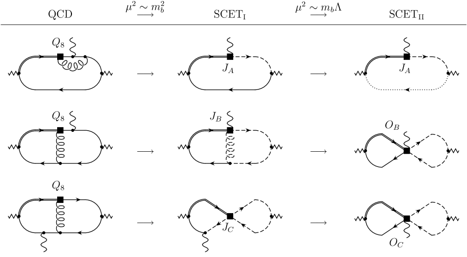
Figure 1: Three QCD Feynman diagrams for the contributions of $Q_{8}$ and their leading-order representation in the effective theory. The double line denotes the heavy-quark field. The dashed lines denote hard-collinear fields in SCET_I and collinear fields in SCET_II. Solid lines in the effective-theory diagrams denote soft fields and the dotted line denotes a soft-collinear field.

Figure 1 shows three typical contributions to the decomposition of the correlator (5), for the chromomagnetic operator $Q_{8}$. The three rows in the figure illustrate the soft-overlap ($A$), hard-scattering ($B$), and spectator-emission ($C$) mechanisms. The two-step matching procedure QCD $\to$ SCET_I $\to$ SCET_II is described in the following Sections 2.2 and 2.3.

Note that the soft-collinear region has $p^{2}\sim\Lambda^{3}/m_{b}\ll\Lambda^{2}$. It has sometimes been argued that it is “unphysical” to allow for momentum regions with $p^{2}$ parametrically below $\Lambda^{2}$, since non-perturbative effects would modify physics below this scale, and that it would therefore be more natural to perform the perturbative factorization analysis with a hard infrared cut-off in QCD. Since the key point in factorization proofs is precisely to show that such infrared regions are either absent or cancel in the sum over diagrams, simply ignoring such modes is clearly not an option. If one chooses to introduce an infrared cut-off in QCD, the proof of factorization becomes equivalent to the demonstration of insensitivity to this regulator. However, it is difficult to introduce such a cut-off in a gauge invariant way, and it is also doubtful whether the diagrammatic analysis with a cut-off can be reformulated in effective-theory language. Since the messenger fields do not contribute (by definition) to factorizable quantities, and since non-factorizable quantities are categorized as non-perturbative, nothing is gained by removing these fields in favor of an infrared cut-off. One of the advantages of the effective-theory approach in dimensional regularization is precisely that the analysis can be performed without explicit momentum cut-offs.

While it is easy to see that all of the above regions are required to obtain the expansion of the correlator diagrams, we do not have a proof that they are sufficient. Two-loop applications in similar kinematic situations [28] suggest that no additional regions are needed. The above list of momentum scalings is natural in that it contains all onshell modes whose components $n\cdot p$ and $\bar{n}\cdot p$ scale with powers of $\lambda$ equal to the scaling of the components of external momenta.

Finally, let us note that the analysis of regions presented above assumes exactly massless light quarks. A systematic inclusion of quark mass terms presents a challenge, since the mode structure in the low-energy theory is then drastically altered. For instance, including ${\cal O}(\Lambda)$ masses would eliminate the soft-collinear mode, but the resulting diagrams for the soft and collinear regions would no longer be separately well-defined in dimensional regularization, requiring additional unconventional (e.g., analytic) regulators. We will return to this issue in Section 4.3 and address the more modest question of the leading corrections for light-quark masses $m_{q}\ll\Lambda$. We argue that contributions linear in the light mass may be absorbed into the hadronic parameters appearing in the factorization formula, while any terms that could potentially spoil factorization appear first at quadratic order.

2.2 Intermediate effective theory: SCET_I

In the construction of the SCET Lagrangian, an effective-theory field is introduced for each momentum region. The integrands of the QCD Feynman diagrams expanded in the various regions are then reinterpreted as arising from the Feynman rules of the effective theory. Furthermore, in order to ensure that the amplitudes are appropriately expanded in momentum space, a derivative (“multipole”) expansion is performed in the effective action.

Note that if we had chosen the momentum of the vector meson to be $n$-hard-collinear, then only the hard, $n$-hard-collinear, $\bar{n}$-hard-collinear, and the soft region would appear in the expansion of (5). It is simpler to first consider the situation where we count the external momenta in this way and to introduce fields only for these regions. This is illustrated by the middle column of Figure 1. The corresponding effective theory, called SCET_I, describes QCD at or below the hard-collinear scale, and contains the quark and gluon fields

$$\xi_{hc} \sim\lambda^{1/2}, A_{hc}^{\mu} \sim(\lambda,1,\sqrt{\lambda}), \xi_{\overline{hc}} \sim\lambda^{1/2}, A_{\overline{hc}}^{\mu} \sim(1,\lambda,\sqrt{\lambda})\,,$$ (8)

$$q_{s} \sim\lambda^{3/2}, A_{s}^{\mu} \sim(\lambda,\lambda,\lambda)\,, h \sim\lambda^{3/2}.$$

The hard-collinear quarks are described by two-component spinors satisfying $n\!\!\!/\,\xi_{hc}=\bar{n}\!\!\!/\,\xi_{\overline{hc}}=0$. We have indicated in (8) the scaling of the field components, which can be derived from the scaling of the corresponding propagators. No field is introduced for the hard region, as this contribution will be absorbed into the Wilson coefficients of operators in the effective theory. As was shown in [5], for diagrams involving only a single type of hard-collinear field, in dimensional regularization there is no hard contribution in the pure QCD sector, since the corresponding diagrams are scaleless and vanish. The effective Lagrangian can then be constructed exactly, to all orders in perturbation theory. This was done to next-to-next-to-leading power in [29]. The same may be done in our case with two types of hard-collinear fields, which we denote generically as $\phi_{hc}$ and $\phi_{\overline{hc}}$. In fact, the Lagrangian for this case is simply

$${\cal L}={\cal L}_{hc}+{\cal L}_{\overline{hc}}+{\cal L}_{s}$$ (9)

where ${\cal L}_{s}$ is given by the HQET Lagrangian for heavy quarks, and by the restriction of the QCD Lagrangian to soft momentum modes for light quarks and gluons. ${\cal L}_{hc}$ denotes the remainder containing the hard-collinear fields and their interactions with the soft fields, and ${\cal L}_{\overline{hc}}$ is obtained from ${\cal L}_{hc}$ by interchanging $n$ and $\bar{n}$.

Figure 2: Example of an exceptional momentum configuration giving rise to an interaction in SCET_I involving $hc$ and $\overline{hc}$ fields.

Note that we did not write down a Lagrangian containing interactions with both $n$- and $\bar{n}$-hard-collinear fields. By the Coleman-Norton theorem [30], pinch singularities can only occur in momentum configurations that can be interpreted as classical scattering processes. By momentum conservation, this cannot occur in interactions with both $n$-hard-collinear and $\bar{n}$-hard-collinear particles unless both types of particles are present in the initial and final states. An example is illustrated in Figure 2, where the momentum $k$ is restricted to the region $k\sim(\lambda,\lambda,\sqrt{\lambda})$. When this skeleton diagram is inserted into loop diagrams, an integration over $k$ in this region involves denominators of the form $(p_{hc\perp}+k_{\perp})^{2}+\bar{n}\cdot p_{hc}n\cdot k$ and $(p_{\overline{hc}\perp}+k_{\perp})^{2}+n\cdot p_{\overline{hc}}\,\bar{n}\cdot k$. The contour integrals in $n\cdot k$ ($\bar{n}\cdot k$) vanish if the external particles all have the same sign of $\bar{n}\cdot p_{hc}$ ($n\cdot p_{\overline{hc}}$), and such exceptional configurations are therefore not relevant in cases where collinear particles are present only in the final state. The absence of such exceptional momentum configurations is encoded automatically in the usual strategy of regions applied to the perturbative expansion of the correlator (5) in dimensional regularization. For an $N$-loop diagram, this strategy assigns onshell momentum scaling to $N$ internal lines, with the scaling of all remaining lines fixed by momentum conservation. The full amplitude is recovered by performing this assignment in all possible ways, with an unrestricted integration over the $N$ onshell loop momenta. With these rules, an isolated offshell line such as in Figure 2 (with momentum $p_{hc}+p_{\overline{hc}}+k$) cannot occur.

It is convenient to use the SCET_I operators to classify the different mechanisms through which the decay $B\rightarrow V\gamma$ can proceed. In contrast to the Lagrangian interactions, there are hard matching corrections to the weak-interaction operators in the effective theory. After performing the matching of QCD onto SCET_I, the remaining problem is to examine in each case all possible SCET_II operators that can result. We now turn to this problem and discuss the issues involved in integrating out the hard-collinear components of the SCET_I fields.

2.3 Final effective theory: SCET_II

Counting the external momenta as collinear, instead of hard-collinear, the full list of regions in Section 2.1 needs to be considered. The dynamical fields in this case are the collinear and soft fields

$$\xi_{c} \sim\lambda\,, A_{c}^{\mu} \sim(\lambda^{2},1,\lambda)\,, q_{s} \sim\lambda^{3/2}, A_{s}^{\mu} \sim(\lambda,\lambda,\lambda)\,, h \sim\lambda^{3/2},$$ (10)

as well as the soft-collinear quark and gluon fields

$$\theta \sim\lambda^{2}, A_{sc}^{\mu} \sim(\lambda^{2},\lambda,\lambda^{3/2})\,.$$ (11)

The collinear and soft-collinear fields are again described by two-component spinors satisfying $\hbox to0.0pt{\hskip 0.56917pt/\hss}{n}\,\xi_{c}=\hbox to0.0pt{\hskip 0.56917pt/\hss}{n}\,\theta=0$. The small-component projection of the soft-collinear fermion field, satisfying $\hbox to0.0pt{\hskip 0.56917pt/\hss}{\bar{n}}\sigma=0$, is given by

$$\sigma=-\frac{\bar{n}\!\!\!/}{2}\frac{1}{i\bar{n}\cdot D_{sc}}{iD\!\!\!\!/}_{sc\perp}\theta\,.$$ (12)

In SCET_II, both the hard and hard-collinear contributions are absorbed into the Wilson coefficients of the operators built from the above fields. The hard-collinear contributions appear in the matching step from SCET_I onto SCET_II. As in the first matching step, the pure QCD part of the effective Lagrangian can be obtained exactly. It was constructed at next-to-leading power in [25].

\psfrag{s}[r]{$(\lambda,\lambda,\lambda)$}\psfrag{c}[l]{$(\lambda^{2},1,\lambda)$}\psfrag{o}[l]{$(\lambda,1,\lambda)$}\includegraphics[width=119.50159pt]{figure3.ps}

Figure 3: Example of a SCET_I diagram relevant for $B\to V\gamma$ decay with an offshell-collinear gluon. The same contribution is also depicted in the second line of Figure 1.

In preparation for the discussion of general operator bases to be considered in Section 3, we review here the procedure employed in integrating out the fields at the hard-collinear scale. We begin by restricting attention to the sector of the SCET_I Lagrangian (9) involving $n$-hard-collinear and soft fields. Just as matching QCD to SCET_I involved decomposing the QCD fields into their hard, hard-collinear, and soft components, so matching onto SCET_II involves the decomposition of SCET_I fields. In particular, a generic hard-collinear field is decomposed as

$$\phi_{hc}\to\phi_{hc}+\phi_{c}+\phi_{oc}\,,$$ (13)

where the hard-collinear, collinear and offshell-collinear momenta scale as $(\lambda,1,\sqrt{\lambda})$, $(\lambda^{2},1,\lambda)$, and $(\lambda,1,\lambda)$, respectively. The latter momentum scaling arises from the combination of onshell soft and collinear momenta, see Figure 3. The hard-collinear and offshell-collinear fields are integrated out in passing from SCET_I to SCET_II, just as the hard components of the QCD fields were integrated out in passing from QCD to SCET_I. Similarly, a generic soft field is decomposed as

$$\phi_{s}\to\phi_{s}+\phi_{sc}\,,$$ (14)

where the soft and soft-collinear momenta scale as $(\lambda,\lambda,\lambda)$ and $(\lambda^{2},\lambda,\lambda^{3/2})$. In contrast to SCET_I, where the soft fields are defined to contain all modes below the soft scale, the soft fields in SCET_II are defined to contain strictly soft, and not soft-collinear modes. This interpretation is mandated by the appearance of a new region in SCET_II. If we were to work with explicit cut-offs, the soft fields would be required to have $n\cdot p_{s}$ of order $\lambda$ (thus excluding modes with $n\cdot p_{s}$ of order $\lambda^{2}$), and collinear fields would be required to have $\bar{n}\cdot p_{c}$ of order unity (excluding modes with $\bar{n}\cdot p_{c}$ of order $\lambda$). The situation is analogous to the passage from QCD to SCET_I, where the hard-collinear region is defined to contain strictly hard-collinear, and not soft, modes.

We now expand the SCET_I Lagrangian (9) using the decompositions (13) and (14). We split the Lagrangian into two parts, one containing the “light” degrees of freedom present in the low-energy theory, and one containing “heavy” modes that are to be integrated out. In the first part, ${\cal L}_{\rm light}$, we collect all terms that contain only fields that are part of SCET_II: soft, collinear, and soft-collinear fields. ${\cal L}_{\rm light}$ has been derived in [25] and is required through ${\cal O}(\lambda)$:

$${\cal L}_{\rm light} = {\cal L}_{s}+{\cal L}_{c}+{\cal L}_{sc}+{\cal L}_{s+sc}^{\rm int}+{\cal L}_{c+sc}^{\rm int}+\dots$$ (15)

$$= {\cal L}_{\rm light}^{(0)}+{\cal L}_{\rm light}^{(1/2)}+{\cal L}_{\rm light}^{(1)}+\dots\,.$$

Terms with both soft and collinear fields appear at subleading power in the decomposition of the SCET_I Lagrangian, both directly in ${\cal L}_{\rm light}$, and via induced interactions after integrating out offshell modes in ${\cal L}_{{\rm heavy}}$ below, as discussed in [6]. However, such interactions are not relevant to our analysis, as they do not appear in the expansion of the correlator (5). More generally, they are absent in cases where collinear particles are present only in the final state, by the same reasoning as for the terms with both $n$-hard-collinear and $\bar{n}$-hard-collinear fields in the decomposition of the QCD Lagrangian in Section 2.2.

In the remaining part of the Lagrangian, ${\cal L}_{{\rm heavy}}$, we collect all terms that involve at least one hard-collinear or offshell-collinear field, which will be integrated out in the construction of SCET_II. For simplicity, in the discussion of Lagrangian terms involving such “heavy” modes, we work in light-cone gauge $\bar{n}\cdot A=0$ for the fields descending from $A_{hc}$ (i.e., hard-collinear, collinear, offshell-collinear), and $n\cdot A=0$ for the fields descending from $A_{s}$ (i.e., soft and soft-collinear). To fully separate the different scales, interactions involving fields with different momentum scaling must be multipole-expanded and the offshell-collinear fields $\xi_{oc}$ and $A_{oc}$ integrated out. The remaining onshell fields can be assigned a definite power counting, and the offshell fields are expressed in terms of a series (ordered in $\lambda$) giving the possible branchings into these onshell fields. For interactions of collinear with hard-collinear fields we have

$$\phi_{hc}(x)\phi_{c}(x)=\phi_{hc}(x)\bigg{[}\phi_{c}(x_{+})+x_{\perp}^{\mu}\partial_{\mu}\phi_{c}(x_{+})+\big{(}{x_{-}^{\mu}\partial_{\mu}}+{1\over 2}x_{\perp}^{\mu}x_{\perp}^{\nu}\partial_{\mu}\partial_{\nu}\big{)}\phi_{c}(x_{+})+\dots\bigg{]}\,.$$ (16)

Similarly, for soft and hard-collinear fields $\phi_{hc}(x)\phi_{s}(x)\approx\phi_{hc}(x)\phi_{s}(x_{-})$, while for soft and collinear fields, $\phi_{s}(x)\phi_{c}(x)\approx\phi_{s}(x_{-}+x_{\perp})\phi_{c}(x_{+}+x_{\perp})$.

We first expand ${\cal L}_{{\rm heavy}}$ in powers of $\lambda$. We begin with the tree level case (i.e., neglecting interactions involving onshell hard-collinear fields), where we will find that the solutions for the offshell fields scale as $\xi_{oc}\sim\lambda^{3/2}$, $A_{oc\perp}^{\mu}\sim\lambda^{3/2}$, and $n\cdot A_{oc}\sim\lambda^{2}$. We will then consider the inclusion of hard-collinear fields, finding that the solutions for the offshell fields in this case start at one power lower in $\lambda$:

$$\xi_{oc} =\big{(}\xi_{oc}^{(1/2)}+\xi_{oc}^{(1)}\big{)}+\xi_{oc}^{(3/2)}+\dots\,,$$ (17)

$$A_{oc\perp} =\big{(}A_{oc\perp}^{(1/2)}+A_{oc\perp}^{(1)}\big{)}+A_{oc\perp}^{(3/2)}+\dots\,,$$

$$n\cdot A_{oc} =\big{(}n\cdot A_{oc}^{(1)}+n\cdot A_{oc}^{(3/2)}\big{)}+n\cdot A_{oc}^{(2)}+\dots\,.$$

The terms in parentheses only appear when branchings into hard-collinear fields are included.

The tree-level Lagrangian begins at ${\cal O}(\lambda)$, and for a complete matching at leading power we require terms through ${\cal O}(\lambda^{3})$. With the inclusion of hard-collinear fields, the Lagrangian begins at one power lower in $\lambda$:

$${\cal L}_{{\rm heavy}}=\left({\cal L}_{{\rm heavy}}^{(0)}+{\cal L}_{{\rm heavy}}^{(1/2)}\right)+{\cal L}_{{\rm heavy}}^{(1)}+\dots\,.$$ (18)

Omitting the terms involving hard-collinear fields for the moment, the leading fermion Lagrangian reads

$${\cal L}_{{\rm heavy}}^{(1)}=\bar{\xi}_{oc}^{(3/2)}{\hbox to0.0pt{\hskip 0.56917pt/\hss}{\bar{n}}\over 2}in\cdot\partial\,\xi_{oc}^{(3/2)}+\big{\{}\bar{\xi}_{oc}^{(3/2)}g\hbox to0.0pt{\hskip 1.9919pt/\hss}{A}_{c\perp}q_{s}+\bar{\xi}_{c}g\hbox to0.0pt{\hskip 1.9919pt/\hss}{A}_{oc\perp}^{(3/2)}q_{s}+\mbox{h.c.}\big{\}}\,,$$ (19)

and solving the equation of motion yields

$$\xi_{oc}^{(3/2)}={-1\over in\cdot\partial}{\hbox to0.0pt{\hskip 0.56917pt/\hss}{n}\over 2}g\hbox to0.0pt{\hskip 1.9919pt/\hss}{A}_{c\perp}q_{s}\,.$$ (20)

Similarly, from the gluon terms in ${\cal L}_{{\rm heavy}}^{(1)}$ we find

$$A_{oc\perp}^{(3/2)\mu} = {g\over i\bar{n}\cdot\partial\,in\cdot\partial}\big{\{}T^{a}\bar{q}_{s}\gamma_{\perp}^{\mu}T^{a}\xi_{c}+\mbox{h.c.}\big{\}}\,,$$

$$n\cdot A_{oc}^{(2)} = {2g\over i\bar{n}\cdot\partial}[A_{c\perp\mu},A_{s\perp}^{\mu}]\,.$$ (21)

Having found the leading terms, these solutions may be substituted back into ${\cal L}_{{\rm heavy}}$, and the process iterated at the next power in $\lambda$. The complete list of SCET_II operators at leading power requires also $\xi_{oc}^{(2)}$ and $\xi_{oc}^{(5/2)}$; these terms themselves involve $A_{oc\perp}^{(2)}$ and $n\cdot A_{oc}^{(5/2)}$. The tree-level expressions were obtained in [11].

Beyond tree level, we must consider the branching of offshell-collinear fields into two or more onshell hard-collinear modes. At each order in $\lambda$, we expand in powers of the coupling constant $g$. Only factors of $g$ associated with hard-scale (i.e., hard-collinear and offshell-collinear) gluons are included in this expansion. Anticipating that $\xi_{oc}^{(1/2)}\sim g$ and $A_{oc\perp}^{(1/2)}\sim g$, contributions to ${\cal L}_{\rm heavy}$ involving offshell-collinear fields begin at ${\cal O}(g^{2})$. For the fermion Lagrangian,

$${\cal L}_{{\rm heavy}}^{(0)} = {\cal L}_{hc}+\bar{\xi}_{oc}^{(1/2)}{\hbox to0.0pt{\hskip 0.56917pt/\hss}{\bar{n}}\over 2}in\cdot\partial\xi_{oc}^{(1/2)}+\bigg{\{}\bar{\xi}_{oc}^{(1/2)}{\hbox to0.0pt{\hskip 0.56917pt/\hss}{\bar{n}}\over 2}\left(g\,n\cdot A_{hc}+g{\hbox to0.0pt{\hskip 1.9919pt/\hss}{A}}_{hc\perp}{1\over i\bar{n}\cdot\partial}i\hbox to0.0pt{\hskip 0.56917pt/\hss}{\partial}_{\perp}\right)\xi_{hc}+\mbox{h.c.}\bigg{\}}$$ (22)

$$\quad+\bar{\xi}_{hc}{\hbox to0.0pt{\hskip 0.56917pt/\hss}{\bar{n}}\over 2}\left(g\,n\cdot A_{oc}^{(1)}+i\hbox to0.0pt{\hskip 0.56917pt/\hss}{\partial}_{\perp}{1\over i\bar{n}\cdot\partial}g\hbox to0.0pt{\hskip 1.9919pt/\hss}{A}_{oc\perp}^{(1/2)}+g\hbox to0.0pt{\hskip 1.9919pt/\hss}{A}_{oc\perp}^{(1/2)}{1\over i\bar{n}\cdot\partial}i\hbox to0.0pt{\hskip 0.56917pt/\hss}{\partial}_{\perp}\right)\xi_{hc}+{\cal O}(g^{3})\,.$$

Solving the equation of motion yields

$$\xi_{oc}^{(1/2)}={-g\over in\cdot\partial}\left(n\cdot A_{hc}+{\hbox to0.0pt{\hskip 1.9919pt/\hss}{A}}_{hc\perp}{1\over i\bar{n}\cdot\partial}i\hbox to0.0pt{\hskip 0.56917pt/\hss}{\partial}_{\perp}\right)\xi_{hc}+{\cal O}(g^{2})\,.$$ (23)

From the gluon terms in ${\cal L}_{{\rm heavy}}^{(0)}$ we find in the same manner

$$A_{oc\perp}^{(1/2)\mu} ={g\over i\bar{n}\cdot\partial\,in\cdot\partial}\bigg{\{}T^{a}\bar{\xi}_{hc}{\hbox to0.0pt{\hskip 0.56917pt/\hss}{\bar{n}}\over 2}\bigg{(}\gamma_{\perp}^{\mu}T^{a}{1\over i\bar{n}\cdot\partial}i\hbox to0.0pt{\hskip 0.56917pt/\hss}{\partial}_{\perp}+i\overleftarrow{\hbox to0.0pt{\hskip 0.56917pt/\hss}{\partial}}_{\perp}{1\over i\bar{n}\cdot\overleftarrow{\partial}}\gamma_{\perp}^{\mu}T^{a}\bigg{)}\xi_{hc}$$

$$\!\!+{1\over 2}[A_{hc\perp}^{\mu},i\bar{n}\cdot\partial n\cdot A_{hc}]-[n\cdot A_{hc},i\bar{n}\cdot\partial A_{hc\perp}^{\mu}]-[A_{hc\perp\nu},i\partial_{\perp}^{\nu}A_{hc\perp}^{\mu}-i\partial_{\perp}^{\mu}A_{hc\perp}^{\nu}]\bigg{\}}+{\cal O}(g^{2})\,,$$

$$n\cdot A_{oc}^{(1)} ={-4g\over(i\bar{n}\cdot\partial)^{2}}\bigg{\{}\frac{1}{2}\left[A_{hc\perp}^{\mu},i\bar{n}\cdot\partial A_{hc\perp\mu}\right]+T^{a}\bar{\xi}_{hc}{\hbox to0.0pt{\hskip 0.56917pt/\hss}{\bar{n}}\over 2}T^{a}\xi_{hc}\bigg{\}}+{\cal O}(g^{2})\,.$$ (24)

Note that the hard-collinear fields appearing on the right-hand side in (23) and (2.3) must have total transverse momentum of order $\lambda$, even though the individual fields have transverse momentum of order $\lambda^{1/2}$. This constraint is automatically enforced by the scaling of external soft and collinear momenta in the evaluation of diagrams corresponding to these interactions. Having derived $\xi_{oc}^{(1/2)}$, $A_{oc\perp}^{(1/2)}$, and $n\cdot A_{oc}^{(1)}$ to the desired order in $g$, these solutions can be substituted back into ${\cal L}_{{\rm heavy}}$, and the procedure iterated at the next order in $\lambda$. This process can be carried out to any order in the power expansion. For offshell-collinear fields branching into hard-collinear fields, the complete list of SCET_II operators at leading power requires also $\xi_{oc}^{(1)}$ and $\xi_{oc}^{(3/2)}$, which themselves involve $A_{oc\perp}^{(1)}$ and $n\cdot A_{oc}^{(3/2)}$. Since further subleading Lagrangian interactions are required to convert the remaining onshell hard-collinear fields into soft and collinear partons, such operators are required only up to one power in $\lambda$ lower than in the tree-level case.

Substituting the expressions (17) for the offshell fields into ${\cal L}_{{\rm heavy}}$ in (18), and inserting appropriate gauge strings to relate the expressions in light-cone gauge to those valid in an arbitrary gauge, yields the final result for the decomposition of the SCET_I Lagrangian in the $n$-hard-collinear sector. The sector of SCET_I involving $\bar{n}$-hard-collinear modes may be treated similarly. It is convenient to treat the photon as being an $\bar{n}$-hard-collinear field in the intermediate effective theory and as an $\bar{n}$-collinear field, $A^{\rm(em)}_{\bar{c}\perp}\sim\lambda$, in SCET_II. The final results are independent of any power counting assigned to this field, since we work to first order in the electromagnetic coupling. As discussed in Section 2.1, no other $\bar{n}$-collinear fields appear in the $B\to V\gamma$ analysis. The decomposition of the SCET_I Lagrangian in this sector is obtained from (18) simply by replacing $n\leftrightarrow\bar{n}$ and dropping all other $\bar{n}$-collinear fields. The same manipulations as in the previous case yield the final result for the explicitly gauge-invariant and multipole-expanded Lagrangian in the sector involving $\bar{n}$-hard-collinear and soft fields. The matching of SCET_I onto SCET_II is completed by substituting the solutions for the offshell fields into external current operators, and integrating out the remaining onshell hard-collinear fields. The hard-collinear modes do not contribute additional renormalizations to the relevant part of the low-energy QCD Lagrangian, but result in non-trivial matching conditions for external currents. This matching is discussed in detail in Section 3.

As an illustration of the passage from SCET_I to SCET_II, we may consider the representation of operators contributing to form-factor matrix elements. The leading-power SCET_I current operators are of the schematic form $\bar{\xi}_{hc}h$. Using the decomposition (13) and enforcing momentum conservation to drop the term involving a single hard-collinear ($hc$) field, the mapping onto SCET_II operators is given by:

$$\bar{\xi}_{hc}h \to\bar{\xi}_{c}h+\bar{\xi}_{oc}h\,.$$ (25)

Expanding the solution of the equation of motion for the field $\bar{\xi}_{oc}$ as in (17), we then have diagrammatically at tree-level:

$$\bar{\xi}_{oc}^{(3/2)}h =\parbox{65.44133pt}{\epsfbox{eqnfig1a.ps}} \equiv\parbox{65.44133pt}{\epsfbox{eqnfig1b.ps}}$$ (26)

$$\bar{\xi}_{oc}^{(2)}h =\parbox{65.44133pt}{\epsfbox{eqnfig2a.ps}} \equiv\parbox{65.44133pt}{\epsfbox{eqnfig2b.ps}}+\parbox{65.44133pt}{\epsfbox{eqnfig2c.ps}}+\parbox{65.44133pt}{\epsfbox{eqnfig2d.ps}}+\parbox{65.44133pt}{\epsfbox{eqnfig2e.ps}}$$

$$\bar{\xi}_{oc}^{(5/2)}h =\parbox{65.44133pt}{\epsfbox{eqnfig3a.ps}} \equiv\parbox{65.44133pt}{\epsfbox{eqnfig3b.ps}}+\quad\parbox{65.44133pt}{\epsfbox{eqnfig3c.ps}}+\parbox{65.44133pt}{\epsfbox{eqnfig3d.ps}}\quad+\quad\dots$$

The contribution of the leading operator $\bar{\xi}_{c}h\sim\lambda^{5/2}$ receives an additional suppression when inserted into correlator diagrams (analogous to Figure 1) for the form factor, because these diagrams will always involve soft-collinear quark lines. For example

$$\bar{\xi}_{c}h =\parbox{65.44133pt}{\epsfbox{eqnfig4a.ps}} \to\parbox{122.34685pt}{\epsfbox{eqnfig4b.ps}}+\parbox{122.34685pt}{\epsfbox{eqnfig4c.ps}}+\quad\dots$$ (27)

With the additional $\lambda^{3/2}$ suppression from subleading Lagrangians terms in ${\cal L}_{\rm light}$ describing the coupling to soft-collinear quarks, the contribution ends up being of order $\lambda^{4}$, the same order as the contribution of $\bar{\xi}_{oc}^{(5/2)}h$. Another example of this additional suppression relating to $B\rightarrow V\gamma$ is illustrated by the first row in Figure 1, where the operator $\bar{\xi}_{c}h$ appears in combination with subleading interpolating current operators for the initial- and final-state mesons that contain soft-collinear quarks. We will discuss this in more detail in Section 3.

The operators from $\bar{\xi}_{oc}^{(5/2)}h\sim\lambda^{4}$ and their leading-order matching coefficients were given in [12]. Additional terms arise at leading power from $\bar{\xi}_{oc}^{(5/2)}h$ for flavor-singlet final-state mesons and have not been shown in (26). As discussed in more detail in Section 3, these terms contain collinear gluon fields in place of the collinear fermion bilinear. For the remaining terms, $\bar{\xi}_{oc}^{(3/2)}h\sim\lambda^{3}$ gives rise to soft-overlap contributions in the flavor-singlet case, connected with terms arising from $\bar{\xi}_{oc}^{(5/2)}h$. Similar to $\bar{\xi}_{c}h$, the operators in $\bar{\xi}_{oc}^{(2)}h\sim\lambda^{7/2}$ receive an ${\cal O}(\lambda^{3/2})$ endpoint suppression, and as a result do not contribute at leading power.

The subleading SCET_I operator $\bar{\xi}_{hc}\overleftarrow{\partial}_{\!\perp}h$ may be decomposed in a similar way:

$$\bar{\xi}_{hc}\overleftarrow{\partial}_{\!\perp}h \to\bar{\xi}_{c}\overleftarrow{\partial}_{\!\perp}h+\bar{\xi}_{oc}\overleftarrow{\partial}_{\!\perp}h\,.$$ (28)

However, in each case the $\partial_{\perp}$ derivative gives an additional ${\cal O}(\lambda)$ suppression relative to the operators in (25). The remaining form-factor contributions of leading power arise from subleading SCET_I operators of the form $\bar{\xi}_{hc}A_{hc\perp}h$. The decomposition in this case is

$$\bar{\xi}_{hc}A_{hc\perp}h \to\bar{\xi}_{hc}A_{hc\perp}h+\bar{\xi}_{c}A_{oc\perp}h+\bar{\xi}_{oc}A_{c\perp}h+\bar{\xi}_{c}A_{c\perp}h+\bar{\xi}_{oc}A_{oc\perp}h\,.$$ (29)

Again, from the expansions (17) we find at tree-level:

$$\bar{\xi}_{c}A_{oc\perp}^{(3/2)}h =\parbox{65.44133pt}{\epsfbox{eqnfig5a.ps}}\quad\equiv\quad\parbox{65.44133pt}{\epsfbox{eqnfig5b.ps}}$$

$$\bar{\xi}_{oc}^{(3/2)}A_{c\perp}h =\parbox{65.44133pt}{\epsfbox{eqnfig6a.ps}}\quad\equiv\quad\parbox{65.44133pt}{\epsfbox{eqnfig6b.ps}}$$

$$\bar{\xi}_{c}A_{c\perp}h =\parbox{65.44133pt}{\epsfbox{eqnfig7.ps}}$$

$$\bar{\xi}_{oc}^{(3/2)}A_{oc\perp}^{(3/2)}h ={\cal O}(\lambda^{9/2})$$ (30)

The operator $\bar{\xi}_{c}A_{oc\perp}^{(3/2)}h\sim\lambda^{4}$ contributes hard-scattering contributions of leading power, while $\bar{\xi}^{(3/2)}_{oc}A_{c\perp}h\sim\lambda^{4}$ contributes only for flavor-singlet final-state mesons. Because of an additional $\lambda^{3/2}$ endpoint suppression, $\bar{\xi}_{c}A_{c\perp}h\sim\lambda^{7/2}$ cannot contribute at leading power. Likewise, the contributions of $\bar{\xi}_{oc}^{(3/2)}A_{oc\perp}^{(3/2)}h\sim\lambda^{9/2}$ are also power-suppressed.

This procedure can be extended beyond tree-level by integrating out the (onshell) hard-collinear modes. For instance, for the first term on the right-hand side of (29),

$$\bar{\xi}_{hc}A_{hc\perp}h=\parbox{65.44133pt}{\epsfbox{eqnfig8a.ps}}\to\parbox{122.34685pt}{\epsfbox{eqnfig8b.ps}}+\quad\dots\quad=\parbox{65.44133pt}{\epsfbox{eqnfig8c.ps}}$$ (31)

There are also contributions where offshell-collinear fields branch into hard-collinear modes. For instance, from the second term on the right-hand side of (25),

$$\bar{\xi}_{oc}^{(1/2)}h=\parbox{65.44133pt}{\epsfbox{eqnfig9.ps}} \to\raisebox{-4.26773pt}{\parbox{122.34685pt}{\epsfbox{eqnfig9a.ps}}}\!\!\!+\dots$$ (32)

$$=\!\!\raisebox{2.84544pt}{\parbox{122.34685pt}{\epsfbox{eqnfig9b.ps}}}\!\!\!+\dots\,\,=\raisebox{0.0pt}{\parbox{65.44133pt}{\epsfbox{eqnfig9c.ps}}}$$

In (32) we have displayed a contribution involving the solution for the offshell-collinear gluon field $A_{oc\perp}^{(1/2)}$ substituted back into ${\cal L}_{\rm heavy}^{(0)}$ in (22). While straightforward in principle, these examples illustrate the nontrivial nature of the SCET_I to SCET_II matching. Instead of explicitly integrating out the hard-collinear modes, in Section 3 we will arrive at the complete SCET_II operator basis using only general properties of the decomposition of SCET_I operators. The general form is required both for explicit computations, and to demonstrate factorization properties, such as the decoupling of leading-power soft-collinear interactions. In contrast to SCET_I, the power counting for operators in SCET_II cannot be deduced simply by inspection of the field content. This is illustrated by the third line of (26): the two operators with an additional gluon field turn out to be of the same order as the four-quark operator, due to the non-localities introduced by integrating out the hard-collinear modes, of virtuality $p^{2}\sim m_{b}\Lambda$. These non-localities manifest themselves as inverse partial derivatives, counting like $\lambda^{-1}$ [6]. The appearance of these derivatives is manifest in (20) and (2.3), the solution of the equations of motion for the offshell-collinear fields. In order to proceed, we require a set of rules that can restrict the appearance of such factors and, more generally, allows us to write down the most general SCET_II operators.

3 SCET representation of the weak Hamiltonian

As discussed in the previous section, the QCD part of the low-energy effective theory does not receive matching corrections and can be constructed exactly. This is not true for the operators in the weak Hamiltonian. For this case we proceed in the usual way: we write down all operators with the correct quantum numbers built from the available fields, and perform perturbative matching to the desired order. Our goal in this section is two-fold: to find the SCET_II operators that contribute to $B\to V\gamma$ decay at leading power, and to construct the SCET_I operators which match onto these SCET_II operators. The utility in identifying the SCET_I operators lies in the fact that the soft-overlap contributions can be isolated already at this stage, before further decomposition into SCET_II fields. The two-step matching procedure is also required for the resummation of large perturbative logarithms, which we address in Section 5. Using building blocks defined below, it is straightforward to write down all SCET_I operators that can contribute up to a given order in $\lambda$. The situation is more complicated for the SCET_II operators: when integrating out hard-collinear modes, inverse derivatives $n\cdot\partial$ on the soft fields appear [6], counting as $\lambda^{-1}$. Despite the presence of such derivatives, we will see that only a finite number of operators can appear to a given order in $\lambda$. A second, practical difficulty is that the leading SCET_II operators are of a much higher order in $\lambda$ than the leading SCET_I operators. For example, treating the photon field as a hard-collinear field in SCET_I and as a collinear field in SCET_II, the leading operator in the intermediate theory contributing to $B\to V\gamma$ counts as $\lambda^{5/2}$, while the leading operators in the final effective theory count as $\lambda^{5}$. Power counting alone does not strongly constrain the possible SCET_I operators, and would leave us with a very large number of operators in the intermediate theory, most of which would turn out to be irrelevant upon matching onto SCET_II. We will find that counting the mass dimension of the SCET_I operators leads to much stronger restrictions.

3.1 Building blocks

A characteristic feature of SCET is that derivatives of the (hard-)collinear fields corresponding to large momentum components are unsuppressed, and operators with an arbitrary number of such derivatives can appear at the same order in the power counting. To account for this, the operators are allowed to be non-local along a light ray: for example, the SCET_I representation of a QCD operator at position $x$ can contain the hard-collinear fields $\phi_{hc}(x+s\bar{n})$, $\phi_{\overline{hc}}(x+rn)$. The Wilson coefficients of the operators are then functions of the light-ray variables ($r$ and $s$ in our example).

To obtain gauge-invariant operators, the fields at different points on the light-ray must be connected by light-like Wilson lines (deviations of such Wilson lines from the light cone can be expanded and appear as power-suppressed operators). Instead of inserting these Wilson lines for each operator, it is simpler to work with building blocks [6, 31] obtained by multiplying the fields by Wilson lines which run along the light-ray to infinity. These building blocks will be invariant under hard-collinear gauge transformations in SCET_I, and under soft and collinear gauge transformations in SCET_II. We choose to work with building blocks that have simple transformations, but are not invariant, under soft and soft-collinear gauge transformations in SCET_I and SCET_II, respectively. Purely gauge-invariant quantities may be obtained by introducing additional soft or soft-collinear Wilson lines, but this will not be necessary for our arguments, and would require the appearance of residual Wilson-line factors in SCET current operators. The building blocks defined here are also easier to work with when performing explicit loop calculations. Thus, for SCET_I, we introduce the fields

$${\mathcal{X}}_{hc}(x) =W^{\dagger}_{hc}(x)\xi_{hc}(x)\,,$$ (33)

$${\mathcal{A}}_{hc}^{\mu}(x) =W^{\dagger}_{hc}(x)\big{[}iD^{\mu}_{hc}(x)\,W_{hc}(x)\big{]}+\frac{\bar{n}^{\mu}}{2}\big{[}W^{\dagger}_{hc}(x)gn\cdot A_{s}(x_{-})W_{hc}(x)-gn\cdot A_{s}(x_{-})\big{]}\,,$$

with $iD^{\mu}_{hc}=i\partial_{\mu}+gA_{hc}$ and Wilson line

$$W_{hc}(x)={\rm\bf P}\,\exp\left(ig\int_{-\infty}^{0}\!ds\,\bar{n}\cdot A_{hc}(x+s\bar{n})\right).$$ (34)

Note that $\bar{n}\cdot{\mathcal{A}}_{hc}^{\mu}(x)=0$. The building blocks for the hard-collinear fields in the opposite direction, $\xi_{\overline{hc}}(x)$ and $A_{\overline{hc}}(x)$, are obtained by interchanging $n$ and $\bar{n}$ (and $x_{-}\to x_{+}$) in the above expressions.

The building blocks of SCET_II are defined in an analogous way. In this case the role of the soft fields is played by the soft-collinear fields, and both the soft and the collinear fields are supplied with Wilson lines:

$${\mathcal{X}}_{c}(x) =W^{\dagger}_{c}(x)\xi_{c}(x)\,,$$ (35)

$${\mathcal{A}}_{c}^{\mu}(x) =W^{\dagger}_{c}(x)\big{[}iD^{\mu}_{c}(x)\,W_{c}(x)\big{]}+\frac{\bar{n}^{\mu}}{2}\big{[}W^{\dagger}_{c}(x)gn\cdot A_{sc}(x_{-})W_{c}(x)-gn\cdot A_{sc}(x_{-})\big{]}\,,$$

$${\mathcal{Q}}_{s}(x) =S^{\dagger}_{s}(x)q_{s}(x)\,,\hskip 56.9055pt{\mathcal{H}}_{s}(x)=S^{\dagger}_{s}(x)h(x)\,,$$

$${\mathcal{A}}_{s}^{\mu}(x) =S^{\dagger}_{s}(x)\big{[}iD^{\mu}_{s}(x)\,S_{s}(x)\big{]}+\frac{n^{\mu}}{2}\big{[}S^{\dagger}_{s}(x)g\bar{n}\cdot A_{sc}(x_{+})S_{s}(x)-g\bar{n}\cdot A_{sc}(x_{+})\big{]}\,.$$

The collinear Wilson line $W_{c}(x)$ is defined in the same way as $W_{hc}(x)$ in (34), except that it is constructed with the collinear instead of the hard-collinear gluon field. The soft Wilson line is

$$S_{s}(x)={\rm\bf P}\,\exp\left(ig\int_{-\infty}^{0}\!dt\,n\cdot A_{s}(x+tn)\right).$$ (36)

For a detailed discussion of the gauge transformation properties of the SCET_II fields and the construction of gauge-invariant building blocks, we refer the reader to [25]. Similar to the building blocks for the $\bar{n}$-hard-collinear fields, ${\mathcal{X}}_{\overline{hc}}(x)$ and ${\mathcal{A}}_{\overline{hc}}(x)$, we will also need SCET_II building blocks for which $n$- and $\bar{n}$-directions are interchanged. The only collinear field in the $\bar{n}$-direction is the photon field. However, we will need the associated soft building blocks with Wilson lines in the $\bar{n}$-direction and will denote them by ${\mathcal{Q}}_{{\bar{s}}}(x)$, ${\mathcal{H}}_{{\bar{s}}}(x)$ and ${\mathcal{A}}_{{\bar{s}}}(x)$.

Arbitrary SCET operators are obtained by combining the above building blocks. In products involving different momentum modes, a derivative expansion of the fields has to be performed [5, 25]. The expansion for fields in SCET_I is as in (16), and for SCET_II we have

$$\phi_{s}(x)\phi_{c}(x)\rightarrow\phi_{s}(x_{-}+x_{\perp})\phi_{c}(x_{+}+x_{\perp})\\ +x_{+}\cdot\partial_{s}\phi_{s}(x_{-}+x_{\perp})\phi_{c}(x_{+}+x_{\perp})+\phi_{s}(x_{-}+x_{\perp})x_{-}\cdot\partial_{c}\phi_{c}(x_{+}+x_{\perp})+\dots\,,$$ (37)

and similarly $\phi_{s}(x)\phi_{sc}(x)\approx\phi_{s}(x)\phi_{sc}(x_{+})$, $\phi_{c}(x)\phi_{sc}(x)\approx\phi_{c}(x)\phi_{sc}(x_{-})$. For our leading-power analysis the derivative terms can be dropped, and we will suppress the $x$-dependence of the various fields in the following.

3.2 Operators in SCET

We now present a general procedure for matching generic SCET_I operators onto SCET_II. The SCET_I operators are products of soft fields and hard-collinear fields in the $n$- and $\bar{n}$-directions; schematically we may write

$${\cal O}=[\text{``soft''}]\times[\text{``$n$-hard-collinear''}]\times[\text{``$\bar{n}$-hard-collinear''}]\,.$$ (38)

Because the SCET_I Lagrangian (9) decomposes into the two hard-collinear sectors, each of the three brackets can be treated separately and they match as follows:

$$\begin{matrix}[\text{``$n$-hard-collinear''}]&\longrightarrow&[\text{``$n$-collinear''}]\times[\text{``soft''}]\times[\text{``soft-collinear''}],\\ [\text{``$\bar{n}$-hard-collinear''}]&\longrightarrow&A_{\bar{c}\perp}^{\rm(em)}\times[\text{``soft''}]\times[\text{``soft-collinear''}],\\ [\text{``soft''}]&\longrightarrow&[\text{``soft''}]\times[\text{``soft-collinear''}].\end{matrix}$$ (39)

Physically, the reason that the sectors match separately can be understood by picturing the decay process: at a certain time, the heavy-quark decays into two energetic partons flying in opposite directions. Each of these two particles can subsequently emit soft and collinear particles, but the energetic particles from opposite directions cannot annihilate each other. This physical picture is formalized by the Coleman-Norton theorem. The fact that the soft sector matches separately follows because the soft fields are not integrated out in the transition to SCET_II. Each soft field in SCET_I is simply replaced by the sum of a soft and a soft-collinear field in SCET_II, see (14).

One complication is that the individual sectors are generally not invariant under soft gauge transformations, while our SCET_II building blocks are invariant. In most cases we can avoid matching non-invariant operators by grouping the “soft” bracket together with either the “$n$-hard-collinear” or “$\bar{n}$-hard-collinear” bracket. In the general case, we can introduce soft Wilson lines to make each sector gauge invariant and remove them after the matching is completed. We shall come back to this point in Section 3.2.2.

3.2.1 Current operators

We first discuss the simplest case, namely SCET_I operators of the form

$${\cal O}=[\text{``soft''}]\times[\text{``$n$-hard-collinear''}]\times A_{\overline{hc}\perp}^{\rm(em)}\,,$$ (40)

where we use the schematic notation of (38) for the special case where only the photon field appears in the “$\bar{n}$-hard-collinear” bracket. These operators arise when the photon is emitted from one of the current quarks, but our discussion does not depend on this fact. The analysis for this case is identical to that for the current operators defining heavy-to-light form factors. The construction of the general SCET_II operator basis relevant at leading power has been performed in [11, 12]. We now rederive these results as a preparation for the general case, and to introduce our method. We start by writing out a list of the lowest-dimension current operators in SCET_I. By momentum conservation, the operators must contain at least one hard-collinear field. We will see below that it is most convenient to classify SCET_I operators according to mass dimension, rather than power counting in $\lambda$. Up to dimension five, we find:

$$d=3:\;\; \bar{\mathcal{X}}_{hc}\,\Gamma^{\prime}\,h\quad(J^{A})\,,$$

$$d=4:\;\; \bar{\mathcal{X}}_{hc}\,{\mathcal{A}}_{hc\perp}\,\Gamma^{\prime}\,h\quad(J^{B})\,,\;\;\;\bar{q}_{s}\,{\mathcal{A}}_{hc\perp}\,\Gamma^{\prime\prime}\,h\,,$$

$$\bar{\mathcal{X}}_{hc}\,{\partial}_{hc\perp}\,\Gamma^{\prime}\,h\,,\;\;\;\bar{\mathcal{X}}_{hc}\,D_{s\perp}\,\Gamma^{\prime}\,h\,,$$

$$d=5:\;\; \bar{\mathcal{X}}_{hc}\,{\mathcal{A}}_{hc\perp}\,{\mathcal{A}}_{hc\perp}\,\Gamma^{\prime}\,h\,,\;\;\;\bar{q}_{s}\,{\mathcal{A}}_{hc\perp}\,{\mathcal{A}}_{hc\perp}\,\,\Gamma^{\prime\prime}\,h\,,$$

$$\bar{\mathcal{X}}_{hc}\,\bar{n}\cdot\partial_{hc}\,n\cdot{\mathcal{A}}_{hc}\,\Gamma^{\prime}\,h\,,\;\;\;\bar{\mathcal{X}}_{hc}\,{1\over\bar{n}\cdot\partial_{hc}}{\hbox to0.0pt{\hskip 0.56917pt/\hss}{\bar{n}}\over 2}\Gamma^{\prime}\,{\mathcal{X}}_{hc}\,\,\bar{\mathcal{X}}_{hc}\,\Gamma^{\prime}\,h\,,$$ (41)

$$\bar{\mathcal{X}}_{hc}\,{1\over\bar{n}\cdot\partial_{hc}}{\hbox to0.0pt{\hskip 0.56917pt/\hss}{\bar{n}}\over 2}\Gamma^{\prime}\,{\mathcal{X}}_{hc}\,\,\bar{q}_{s}\,\Gamma^{\prime\prime}\,h\,,\;\;\;\bar{q}_{s}\,\bar{n}\cdot\partial_{hc}\,n\cdot{\mathcal{A}}_{hc}\,\Gamma^{\prime\prime}\,h\,,$$

$$\bar{q}_{s}\,\bar{n}\cdot\partial_{hc}\,{\mathcal{A}}_{hc\perp}\,\frac{\hbox to0.0pt{\hskip 0.56917pt/\hss}{n}}{2}\Gamma^{\prime}\,h\,,\;\dots\,.$$

The symbols in parentheses, $J^{A}$ and $J^{B}$, anticipate the notation to be introduced in Section 4 for the relevant SCET_I operators. We do not display transverse Lorentz indices or color indices; the former may be contracted with the metric and epsilon tensor in the transverse plane,

$$g_{\perp}^{\mu\nu}=g^{\mu\nu}-\frac{1}{2}(\bar{n}^{\mu}n^{\nu}+n^{\mu}\bar{n}^{\nu})\,,\qquad\epsilon_{\perp}^{\mu\nu}=\frac{1}{2}\epsilon^{\mu\nu\alpha\beta}\,{\bar{n}}_{\alpha}n_{\beta}\,.$$ (42)

We use the convention $\epsilon^{0123}=-1$. In the schematic notation of (3.2.1), it is understood that hard-collinear derivatives can act on any of the hard-collinear fields in the operators, and similarly for soft derivatives. We do indicate the Dirac structures that can occur in the above expressions, using the following Dirac matrices that are invariant under the “boost” $n_{\mu}\rightarrow\alpha n_{\mu}$ and $\bar{n}_{\mu}\rightarrow\alpha^{-1}\bar{n}_{\mu}$:

$$\Gamma^{\prime} =\{1,\gamma_{5},\gamma_{\perp}^{\mu}\}\,,$$ (43)

$$\Gamma^{\prime\prime} =\Gamma^{\prime}\cup\{\bar{n}\!\!\!/\,n\!\!\!/,\gamma_{\perp}^{\mu}\gamma_{5},\gamma_{\perp}^{\mu}\gamma_{\perp}^{\nu}-\gamma_{\perp}^{\nu}\gamma_{\perp}^{\mu}\}\,.$$

The sixteen matrices $\hbox to0.0pt{\hskip 0.56917pt/\hss}{n}\Gamma^{\prime}$, $\hbox to0.0pt{\hskip 0.56917pt/\hss}{\bar{n}}\Gamma^{\prime}$, and $\Gamma^{\prime\prime}$ form a Dirac basis. We only consider boost-invariant operators; such a choice is always possible and is also natural because the operators we reproduce with the effective theory are independent of the reference vectors $n_{\mu}$ and $\bar{n}_{\mu}$. Operators that are not boost-invariant can be eliminated in favor of invariant operators obtained by multiplying them with an appropriate number of derivatives $\bar{n}\cdot\partial_{hc}$. The last five operators of dimension five are examples where such derivatives have been included. The presence of these derivatives can be compensated by the Wilson coefficients of the non-local operators, for example

$$\int ds\,C(s)\,\bar{n}\cdot\partial_{hc}\phi_{hc}(x+s\bar{n})\phi_{s}(x)=-\int ds\frac{\partial C(s)}{\partial s}\,\phi_{hc}(x+s\bar{n})\phi_{s}(x)\,.$$ (44)

We did not allow for operators which explicitly involve the vector $v_{\mu}$ in (3.2.1) because it can be eliminated in favor of $\bar{n}_{\mu}$, cf. (6). Furthermore, we have used the projection properties of the spinors $\hbox to0.0pt{\hskip 0.56917pt/\hss}{v}h=h$, $\hbox to0.0pt{\hskip 0.56917pt/\hss}{n}{\mathcal{X}}_{hc}=0$ to eliminate occurrences of $\hbox to0.0pt{\hskip 0.56917pt/\hss}{\bar{n}}\,h$. For instance, the third operator for $d=5$ is obtained by rearranging an operator with $d=4$:

$$\bar{\mathcal{X}}_{hc}\,\Gamma^{\prime}\,{\hbox to0.0pt{\hskip 0.56917pt/\hss}{\bar{n}}\over 2}\,n\cdot{\mathcal{A}}_{hc}\,h =\bar{\mathcal{X}}_{hc}\,\Gamma^{\prime}\,\left(\hbox to0.0pt{\hskip 0.56917pt/\hss}{v}-{\hbox to0.0pt{\hskip 0.56917pt/\hss}{n}\over 2n\cdot v}\right){1\over n\cdot v}\,n\cdot{\mathcal{A}}_{hc}\,h=\frac{1}{n\cdot v}\bar{\mathcal{X}}_{hc}\,\Gamma^{\prime}\,n\cdot{\mathcal{A}}_{hc}\,h$$ (45)

$$\to\bar{\mathcal{X}}_{hc}\,i\bar{n}\cdot\partial_{hc}\,n\cdot{\mathcal{A}}_{hc}\,\Gamma^{\prime}\,h\,.$$

In the second line, we have absorbed a factor $(i\bar{n}\cdot\partial\,n\cdot v)^{-1}$ into the Wilson coefficient of the operators, as in (44). To minimize the list of possible SCET_I operators appearing with a given dimension, it is convenient to always make use of such rearrangements.

For contributions arising at leading power, the SCET_I operators should not contain soft fields in addition to those found in the final SCET_II operators. Such soft fields would not participate in the matching, and result in a power suppression relative to the corresponding operators without the additional soft fields. Similar arguments apply to power-suppressed soft or collinear derivatives; an explicit example of this effect was mentioned in (28) of Section 2.3. Thus only the first two operators for $d=4$ can be relevant for our leading-power analysis. We have also not listed operators of any dimension containing additional factors of $\bar{n}\cdot D_{s}/\bar{n}\cdot\partial_{hc}$. The ellipsis for $d=5$ denotes similarly irrelevant terms.

	$d$	$[\lambda]$
$\frac{1}{\bar{n}\cdot\partial_{c}}\,\bar{\mathcal{X}}_{c}\frac{\bar{n}\!\!\!/}{2}\Gamma^{\prime}{\mathcal{X}}_{c}$	2	2
$\frac{1}{n\cdot\partial_{s}}\,\bar{\mathcal{Q}}_{s}\frac{n\!\!\!/}{2}\Gamma^{\prime}{\mathcal{Q}}_{s}$	2	2
$\bar{\mathcal{Q}}_{s}\Gamma^{\prime\prime}{\mathcal{Q}}_{s}$	3	3
$\!\!{n\!\cdot\!\partial_{s}}\,\bar{\mathcal{Q}}_{s}\frac{\bar{n}\!\!\!/}{2}\Gamma^{\prime}{\mathcal{Q}}_{s}\!\!$	4	4

	$d$	$[\lambda]$
$g_{\perp}^{\mu\nu}$, $\epsilon_{\perp}^{\mu\nu}$	0	0
$\partial_{c\perp}^{\mu}$, ${\mathcal{A}}_{c\perp}^{\mu}$, $\partial_{s\perp}^{\mu}$, ${\mathcal{A}}_{s\perp}^{\mu}$	1	1
$\!\!{n\!\cdot\!\partial_{s}}\bar{n}\!\cdot\!\partial_{s}$, ${n\!\cdot\!\partial_{s}}\bar{n}\!\cdot\!{\mathcal{A}}_{s}\!\!$	2	2
$\!\!{\bar{n}\!\cdot\!\partial_{c}}n\!\cdot\!\partial_{c}$, ${\bar{n}\!\cdot\!\partial_{c}}\,n\!\cdot\!{\mathcal{A}}_{c}\!\!$	2	2
$\frac{1}{\bar{n}\cdot\partial_{c}\,n\cdot\partial_{s}}$	$-2$	$-1$

Table 1: Boost-invariant building blocks for SCET_II operators, with their dimension $d$ and order $[\lambda]$ in the power expansion. Soft derivatives $\partial_{s}$ can act on any soft field in the operator, collinear derivatives $\partial_{c}$ on any collinear field. $\Gamma^{\prime}$ and $\Gamma^{\prime\prime}$ are defined in (43), while $g_{\perp}^{\mu\nu}$ and $\epsilon_{\perp}^{\mu\nu}$ are defined in (42). Additional building blocks are obtained by hermitian conjugation or by replacing ${\mathcal{Q}}_{s}$ with ${\mathcal{H}}_{s}$.

In order to construct all SCET_II operators up to a given power, we work with the set of building blocks in Tables 1 and 2, which are invariant under soft and collinear gauge transformations. Again, we choose to work with boost-invariant quantities. We will begin by using Table 1 to describe the matching onto SCET_II operators corresponding to “typical” momentum configurations in which the partons in the initial- and final-state mesons all carry ${\cal O}(1)$ fractions of the total soft and collinear momenta, respectively. Such configurations are represented by operators with fermion content $\bar{{\mathcal{X}}}_{c}(\dots){\mathcal{X}}_{c}\bar{{\mathcal{Q}}}_{s}(\dots){\mathcal{H}}_{s}$. We will then consider “endpoint” configurations using the generalization in Table 2. These configurations occur when the momentum fraction carried by one of the partons tends to zero, so that the parton may be absorbed from the initial into the final state without hard momentum transfer. In particular, we will find configurations represented by operators with fermion content $\bar{\mathcal{X}}_{c}(\dots){\mathcal{H}}_{s}$. In both cases, using the counting rules for the building blocks containing soft-collinear fields described by the second column in Table 2, we will show that the operators representing the weak current at leading power do not contain soft-collinear modes. At leading power, soft-collinear modes appear only in time-ordered products of the weak current with subleading SCET_II Lagrangian interactions, and with subleading terms in the interpolating currents for the meson states.

The presence of the building block $(n\cdot\partial_{s}\,\bar{n}\cdot\partial_{c})^{-1}$, which counts as an inverse power of $\lambda$, is troubling at first sight. Naively, one could think that there would be infinitely many operators of a given dimension and order in $\lambda$. However, this is not the case: if an inverse derivative $(n\cdot\partial_{s}\,\bar{n}\cdot\partial_{c})^{-1}$ is added to a given operator, then it is necessary to also add two other building blocks with $d=1$ or one building block with $d=2$ at the same time to obtain an operator of the same dimension. As is evident from the tables, this inevitably makes the resulting operator at least one power in $\lambda$ higher than the operator without the inverse derivative. In fact, from Table 1 we see that for operators involving only soft and collinear fields, with zero fermion number in both the soft and collinear sectors, the difference between the dimension of the SCET_I operators and the order in SCET_II power counting is given precisely by the number of occurrences of the building block $(n\cdot\partial_{s}\,\bar{n}\cdot\partial_{c})^{-1}$.

We focus first on the case of flavor non-singlet final states and will then discuss the modifications necessary for the flavor-singlet case. We begin by considering SCET_II operators with fermion field content $\bar{\mathcal{X}}_{c}(\dots){\mathcal{X}}_{c}\,\bar{\mathcal{Q}}_{s}(\dots){\mathcal{H}}_{s}$, corresponding to “typical” partonic configurations inside the initial- and final-state soft and collinear mesons. Using Table 1, and the fact that SCET_I operators have dimension $d\geq 3$, it follows that leading-power contributions from these configurations are ${\cal O}(\lambda^{4})$. Later we will discuss other possible “endpoint” configurations, finding that they also appear at the same order in power counting. From Table 1 we see that with the exception of $(n\cdot\partial_{s}\,\bar{n}\cdot\partial_{c})^{-1}$, the building blocks satisfy $[\lambda]\geq d$, so that leading-power operators of a given dimension must be generated with the minimal number of occurrences of this building block. Starting with the SCET_I operator in (3.2.1) of dimension three, we find that the appropriate fermion field content cannot be obtained while remaining at $d=3$ without at least one occurrence of the inverse derivative. The two possibilities at ${\cal O}(\lambda^{4})$ are then

$$J^{A}\to\frac{1}{\bar{n}\cdot\partial_{c}\,n\cdot\partial_{s}}\,\bigg{[}{1\over\bar{n}\cdot\partial_{c}}\bar{\mathcal{X}}_{c}\frac{\bar{n}\!\!\!/}{2}\Gamma^{\prime}{\mathcal{X}}_{c}\bigg{]}\;\bigg{[}\frac{1}{n\cdot\partial_{s}}\,\bar{\mathcal{Q}}_{s}\frac{n\!\!\!/}{2}\Gamma^{\prime}{\mathcal{H}}_{s}\bigg{]}\,\big{\{}\partial_{c\perp}^{\mu},\;{\mathcal{A}}_{c\perp}^{\mu},\;\partial_{s\perp}^{\mu},\;{\mathcal{A}}_{s\perp}^{\mu}\big{\}}\,$$ (46)

and

$$J^{A}\to\frac{1}{\bar{n}\cdot\partial_{c}\,n\cdot\partial_{s}}\,\bigg{[}{1\over\bar{n}\cdot\partial_{c}}\bar{\mathcal{X}}_{c}\frac{\bar{n}\!\!\!/}{2}\Gamma^{\prime}{\mathcal{X}}_{c}\bigg{]}\;\bar{\mathcal{Q}}_{s}\Gamma^{\prime\prime}{\mathcal{H}}_{s}\,.$$ (47)

As in the tables, the notation is schematic: it is understood that the soft derivatives can act on any of the soft fields, and the collinear derivatives on any of the collinear fields. Using the equation of motion for the soft light-quark field, the above possibilities result in four independent operators, whose explicit forms are given in [12]. Their matrix elements can be expressed in terms of (endpoint divergent) convolution integrals involving twist-2 and twist-3, two- and three-particle LCDAs of the $B$ meson and the light meson. The matching relations (46) and (47) are represented by the term $\bar{\xi}_{oc}^{(5/2)}h$, shown at tree level in (26).

Next, let us consider the SCET_I current operators of dimension four. First, we observe that the operator $\bar{q}_{s}{\cal A}_{hc\perp}\Gamma^{\prime\prime}h$ does not match onto a leading order SCET_II operator. Its soft bracket $\bar{q}_{s}\Gamma^{\prime\prime}h$ is of order $\lambda^{3}$ and remains unchanged in the matching. The gluon field ${\cal A}_{hc\perp}$ must then match onto a $d=1$ operator with collinear field content $\bar{{\mathcal{X}}}_{c}(\dots){\mathcal{X}}_{c}$. Inspection of the table shows that such an operator is of order $\lambda^{2}$, making the overall operator subleading. The only possibility to obtain a leading SCET_II operator at $d=4$ is

$$J^{B}\to\bigg{[}{1\over\bar{n}\cdot\partial_{c}}\bar{\mathcal{X}}_{c}\frac{\bar{n}\!\!\!/}{2}\Gamma^{\prime}{\mathcal{X}}_{c}\bigg{]}\;\bigg{[}\frac{1}{n\cdot\partial_{s}}\,\bar{\mathcal{Q}}_{s}\frac{n\!\!\!/}{2}\Gamma^{\prime}{\mathcal{H}}_{s}\bigg{]}\,.$$ (48)

At tree level, the matching (48) is represented by the term $\bar{\xi}_{c}A_{oc\perp}^{(3/2)}h$ in (31). At dimension five there are no possibilities for leading-power SCET_II operators, due to the constraint $[\lambda]\geq d$. We thus need the SCET_I operators only through $d=4$ for leading-power matching. Finally, from the second column in Table 2, we note that replacing any of the soft or collinear fields in (46), (47), or (48) by soft-collinear fields results in power suppression.

	$d$	$[\lambda]$
${\mathcal{X}}_{c}$	$\frac{3}{2}$	$1$
${1\over\bar{n}\cdot\partial_{c}}{\not{\bar{n}}\over 2}$	$-1$	$0$
${\mathcal{Q}}_{s}$	$\frac{3}{2}$	$\frac{3}{2}$
${1\over n\cdot\partial_{s}}{\not{n}\over 2}$	$-1$	$-1$
$\Gamma^{\prime\prime}$	0	0

	$d$	$[\lambda]$
$\theta$	$\frac{3}{2}$	2
$\sigma$	$\frac{3}{2}$	$\frac{5}{2}$
$D_{sc\perp}^{\mu}\!\!$	1	$\frac{3}{2}$
${\bar{n}\!\cdot\!\partial_{c}}n\!\cdot\!D_{sc}$	2	2
${n\!\cdot\!\partial_{s}}\bar{n}\!\cdot\!D_{sc}$	2	2

Table 2: Boost-invariant building blocks for SCET_II operators containing non-zero fermion number and/or soft-collinear fields. The Dirac structures $\Gamma^{\prime\prime}$ are defined in (43). $\sigma$ is the small-component projection of the soft-collinear fermion, as in (12).

Our analysis has so far relied on the assumption that the field content of the SCET_II operator is $\bar{\mathcal{X}}_{c}(\dots){\mathcal{X}}_{c}\,\bar{\mathcal{Q}}_{s}(\dots){\mathcal{H}}_{s}$, corresponding to “typical” parton configurations. We now consider possible “endpoint”  contributions, corresponding to SCET_II operators with fermion field content $\bar{\mathcal{X}}_{c}(\dots){\mathcal{H}}_{s}$. For this purpose, we consider the building blocks in the first column of Table 2, which generalize the first column of Table 1 to allow the possibility of non-zero fermion number in the soft and collinear sectors. Starting with the SCET_I operator in (3.2.1) of dimension three, the leading SCET_II operator is

$$J^{A}\to\bar{\mathcal{X}}_{c}\Gamma^{\prime}{\mathcal{H}}_{s}\sim\lambda^{5/2}\,.$$ (49)

Again, from the second column in Table 2 we note that replacing any of the soft or collinear fields in (49) by soft-collinear fields results in power suppression. The operator in (49) can yield a leading-power contribution to the form-factor analogue of the correlator (5) when combined with leading-power meson currents and subleading Lagrangian interactions involving the soft-collinear modes [12]. Essentially, these interactions are summarized by the term $S^{\rm induced(3/2)}_{s+c}$ in the effective action of [25]. Leading contributions can also arise from subleading meson currents and leading Lagrangian interactions. A contribution of this type to the $B\to K^{*}\gamma$ amplitude is illustrated in the first line of Figure 1. The interpolating current for the $B$ meson takes the form

$$\bar{b}\gamma_{5}q\to \bar{{\mathcal{H}}}_{s}\Gamma^{\prime\prime}{\mathcal{Q}}_{s} + \bar{{\mathcal{H}}}_{s}\Gamma^{\prime\prime}\theta + \bar{{\mathcal{H}}}_{s}\Gamma^{\prime\prime}\sigma + \dots$$ (50)

$$\sim \quad\lambda^{3} + \lambda^{7/2} + \lambda^{4} + \dots\,,$$

where the small-component projection $\sigma$ of the soft-collinear fermion field is related to $\theta$ as in (12). Similarly for the light meson, taking for example the pseudoscalar case,

$$\bar{q}\gamma_{5}{\hbox to0.0pt{\hskip 0.56917pt/\hss}{\bar{n}}\over 2}q\to \bar{{\mathcal{X}}}_{c}{\hbox to0.0pt{\hskip 0.56917pt/\hss}{\bar{n}}\over 2}\Gamma^{\prime}{\mathcal{X}}_{c} + \bar{\theta}{\hbox to0.0pt{\hskip 0.56917pt/\hss}{\bar{n}}\over 2}\Gamma^{\prime}{\mathcal{X}}_{c} + \dots$$ (51)

$$\sim \quad\lambda^{2} + \lambda^{3} + \dots\,.$$

The subleading currents for both mesons suppress the contribution of $\bar{\mathcal{X}}_{c}\Gamma^{\prime}{\mathcal{H}}_{s}$ by $\lambda^{3/2}$, so that it ends up being of the same order as the contribution of the four-quark operators. Finally, mixed cases can also occur, where an ${\cal O}(\lambda^{1/2})$, or ${\cal O}(\lambda)$, suppressed meson current from (50) or (51) is combined with an ${\cal O}(\lambda)$, or ${\cal O}(\lambda^{1/2})$, suppressed Lagrangian interaction, respectively. The relevant Lagrangian interactions in this case are given by ${\cal L}_{c+sc}^{\rm int}$ and ${\cal L}_{s+sc}^{\rm int}$ in [25]. By the same reasoning, we find that all such endpoint configurations arising from the $d=4$ SCET_I operator $J^{B}$ in (3.2.1) are power suppressed.

Before ending our discussion of heavy-to-light form factors, we consider the case of flavor-singlet final states. Operators corresponding to “typical” partonic configurations again have zero collinear fermion number, but may contain collinear gluon degrees of freedom in place of the fermion bilinear $\bar{{\mathcal{X}}}_{c}(\dots){\mathcal{X}}_{c}$. Requiring also that the collinear fields carry the appropriate twist and color quantum numbers to have overlap with the final-state collinear meson, there must be at least two such collinear gluon fields. From Table 1 we see that the new operators are obtained by the replacements

$$\bigg{[}{1\over\bar{n}\cdot\partial_{c}}\bar{\mathcal{X}}_{c}\frac{\bar{n}\!\!\!/}{2}\Gamma^{\prime}{\mathcal{X}}_{c}\bigg{]}\big{\{}\partial_{c\perp}^{\mu},\;{\mathcal{A}}_{c\perp}^{\mu},\;\partial_{s\perp}^{\mu},\;{\mathcal{A}}_{s\perp}^{\mu}\big{\}}\to\left\{\begin{matrix}{\mathcal{A}}_{c\perp}{\mathcal{A}}_{c\perp}\big{\{}\partial_{c\perp}^{\mu},\;{\mathcal{A}}_{c\perp}^{\mu},\;\partial_{s\perp}^{\mu},\;{\mathcal{A}}_{s\perp}^{\mu}\big{\}}\,,\\ \bar{n}\cdot\partial_{c}n\cdot{\mathcal{A}}_{c}\,{\mathcal{A}}_{c\perp}\end{matrix}\right\}$$ (52)

in (46), and by the replacement

$$\bigg{[}{1\over\bar{n}\cdot\partial_{c}}\bar{\mathcal{X}}_{c}\frac{\bar{n}\!\!\!/}{2}\Gamma^{\prime}{\mathcal{X}}_{c}\bigg{]}\to{\mathcal{A}}_{c\perp}{\mathcal{A}}_{c\perp}$$ (53)

in (47) and (48). From the leading SCET_I current, there will also be new SCET_II operators that combine with subleading soft-collinear Lagrangian interactions and meson currents to yield leading-power contributions. From Tables 1 and 2, we find that at leading power the new operators are obtained by the replacement

$$\bar{\mathcal{X}}_{c}\to\bar{\mathcal{Q}}_{s}{1\over n\cdot\partial_{s}}{\hbox to0.0pt{\hskip 0.56917pt/\hss}{n}\over 2}{\mathcal{A}}_{c\perp}$$ (54)

in (49). Although the right-hand side of (54) scales as $\lambda^{3/2}$ (compared to the left-hand side, which scales as $\lambda$), leading contributions to form-factor matrix elements may still be obtained from subleading Lagrangian interactions involving the soft-collinear modes, which in this case are essentially summarized by the term $S_{s+c}^{{\rm induced}(1)}$ of the effective action in [25].

3.2.2 General operators

After this warm-up, we are ready to discuss the general case where the photon is not necessarily part of the SCET_I operator. The new operators appearing in this case correspond to photon emission from the spectator quark. The argumentation will be similar to the previous section; however, we will have to match also the $\bar{n}$-hard-collinear part in (39):

$$\begin{matrix}[\text{``$\bar{n}$-hard-collinear''}]\to A_{\bar{c}\perp}^{\rm(em)}\times[\text{``soft''}]\times[\text{``soft-collinear''}]\,.\end{matrix}$$ (55)

The building blocks needed in this case are obtained from Tables 1 and 2 by exchanging $n$ and $\bar{n}$, dropping the collinear quark fields, and replacing the collinear gluon with the photon field. Note that the definition of the soft fields then involves Wilson lines in the $\bar{n}$-direction. To distinguish them from the soft-fields appearing in conjunction with the $n$-collinear sector, we denote them by ${\mathcal{H}}_{\bar{s}}$, ${\mathcal{Q}}_{\bar{s}}$, and ${\mathcal{A}}_{\bar{s}}$. We also recall that the SCET_I building blocks introduced in (33) are not invariant under soft gauge transformations; strictly gauge-invariant combinations are given by

$${\mathcal{X}}^{(0)}_{hc}(x)=S_{s}^{\dagger}(x_{-}){\mathcal{X}}_{hc}(x)\,,\quad{\mathcal{A}}_{hc}^{(0)\mu}(x)=S_{s}^{\dagger}(x_{-}){\mathcal{A}}_{hc}^{\mu}(x)S_{s}(x_{-})\,,$$ (56)

with the soft Wilson line defined in (36). In general, the fields contained in the “$n$-hard-collinear” and “$\bar{n}$-hard-collinear” brackets in (38) are not separately gauge-invariant. In order to match onto the building blocks in Tables 1 and 2 in the general case, we first translate to the gauge-invariant combinations appearing in (56).

Let us again start by writing down a list of the relevant SCET_I operators. By momentum conservation, they must have at least one $n$-hard-collinear and one $\bar{n}$-hard-collinear field in addition to the heavy-quark field, and therefore start with dimension $d=d_{n}+d_{\bar{n}}\,(+d_{s})=4$:

$$d=4 =\left\{\begin{matrix}\phantom{0}3+1:&&\phantom{123456789}\bar{\mathcal{X}}_{hc}\,{\mathcal{A}}_{\overline{hc}\perp}\,\Gamma^{\prime}\,h\quad(J^{A})\,,\\ \phantom{0}1+3:&&\phantom{123456789}\bar{\mathcal{X}}_{\overline{hc}}{\mathcal{A}}_{hc\perp}\,\Gamma^{\prime}\,h\quad(J^{D})\,,\end{matrix}\right.$$ (57)

$$d=5 =\left\{\begin{matrix}4+1:&\phantom{123456}\bar{\mathcal{X}}_{hc}\,{\mathcal{A}}_{hc\perp}\,{\mathcal{A}}_{\overline{hc}\perp}\,\Gamma^{\prime}\,h\quad(J^{B})\,,&\\[6.0pt] 3+2:&\bar{\mathcal{X}}_{hc}\,{\mathcal{A}}_{\overline{hc}\perp}\,{\mathcal{A}}_{\overline{hc}\perp}\,\Gamma^{\prime}\,h\,,&\bigg{[}{1\over n\cdot\partial_{\overline{hc}}}\bar{\mathcal{X}}_{\overline{hc}}\,\frac{\not{n}}{2}\,\Gamma^{\prime}\,{\mathcal{X}}_{\overline{hc}}\bigg{]}\,\,\bar{\mathcal{X}}_{hc}\,\Gamma^{\prime}\,h\,,\\[6.0pt] 2+3:&\bigg{[}{1\over\bar{n}\cdot\partial_{hc}}\bar{\mathcal{X}}_{hc}\,\frac{\not{\bar{n}}}{2}\,\Gamma^{\prime}\,{\mathcal{X}}_{hc}\bigg{]}\,\,\bar{\mathcal{X}}_{\overline{hc}}\,\Gamma^{\prime}\,h\quad(J^{C})\,,&\bar{\mathcal{X}}_{\overline{hc}}\,{\mathcal{A}}_{hc\perp}\,{\mathcal{A}}_{hc\perp}\,\Gamma^{\prime}\,h\quad(J^{E})\,,\\[6.0pt] 1+4:&\bar{\mathcal{X}}_{\overline{hc}}\,{\mathcal{A}}_{\overline{hc}\perp}\,{\mathcal{A}}_{hc\perp}\,\Gamma^{\prime}\,h\,,&\\[6.0pt] 1+1+3:&\bar{q}_{s}\,{\mathcal{A}}_{hc\perp}\,{\mathcal{A}}_{\overline{hc}\perp}\,\Gamma^{\prime\prime}\,h\,.&\end{matrix}\right.$$

The symbols $J^{A},\dots,J^{E}$ in parentheses anticipate the notation to be introduced for these operators in Section 4. In constructing this list, we made the same simplifications as in (3.2.1) for the form-factor case. In the above operators the field ${\mathcal{A}}_{\overline{hc}}$ stands for either the photon or a gluon field, which are treated on the same footing. In SCET_II, we treat the photon as a collinear field in the $\bar{n}$ direction, ${\mathcal{A}}_{{\bar{c}}\perp}^{(\rm em)}\sim\lambda$. Since it appears only once in each operator, we are free to make such a scaling assignment.

In the above list of operators, we have separately indicated the mass dimensions of fields in the $n$-hard-collinear, $\bar{n}$-hard-collinear, and soft brackets, respectively. In those cases where the only soft field is the heavy-quark field, we have included it in one of the hard-collinear sectors in such a way that both hard-collinear brackets carry zero fermion number. SCET_II operators with zero fermion number can be constructed from the building blocks in Table 1 which fulfill $[\lambda]\geq d$. Beyond $d=5$, operators appear which cannot be arranged to have zero fermion number in each hard-collinear sector. For example,

$$d=6:\qquad\bar{\mathcal{X}}_{hc}\,\Gamma^{\prime}\,{\mathcal{X}}_{\overline{hc}}\,\,\bar{\mathcal{X}}_{hc}\,\Gamma^{\prime}\,h\,,\qquad\bar{\mathcal{X}}_{\overline{hc}}\,\Gamma^{\prime}{\mathcal{X}}_{hc}\,\,\bar{\mathcal{X}}_{\overline{hc}}\,\Gamma^{\prime}\,h\,,\dots\,.$$ (58)

In Table 2 we have generalized the first column of Table 1 to include building blocks with non-zero fermion number, by splitting the various fermion bilinears in two halves in all possible boost-invariant ways. With the exception of ${\mathcal{X}}_{c}$, all building blocks again satisfy $[\lambda]\geq d$. In fact, since $\bar{{\mathcal{X}}}_{c}\Gamma^{\prime\prime}{\mathcal{X}}_{c}=0$, the operator constructed from the $n$- and $\bar{n}$-hard-collinear sectors must contain a factor $(\bar{n}\cdot\partial_{c})^{-1}\hbox to0.0pt{\hskip 0.56917pt/\hss}{\bar{n}}/2$, so that the bound $[\lambda]\geq d$ is recovered in the final operator. SCET_I operators with $d\geq 6$ are therefore not relevant to a leading-power analysis.

For the $n$-hard-collinear sector, we may use Table 1 to list the leading-order matching relations onto operators with minimal collinear field content $\bar{\mathcal{X}}_{c}(\dots){\mathcal{X}}_{c}$. This yields:

$$d_{n}=1:\;{\mathcal{A}}_{hc\perp} \to S_{s}\left(\frac{1}{\bar{n}\cdot\partial_{c}n\cdot\partial_{s}}\bigg{[}\frac{1}{\bar{n}\cdot\partial_{c}}\,\bar{\mathcal{X}}_{c}\frac{\bar{n}\!\!\!/}{2}\Gamma^{\prime}{\mathcal{X}}_{c}\bigg{]}{\mathcal{A}}_{s\perp}\right)S_{s}^{\dagger} \!\!\!\!\!\sim\lambda^{2}$$

$$d_{n}=2:\;\left\{\begin{matrix}{\mathcal{A}}_{hc\perp}{\mathcal{A}}_{hc\perp}\,,\\[6.0pt] {1\over\bar{n}\cdot\partial_{hc}}\bar{\mathcal{X}}_{hc}{{\not\bar{n}}\over 2}\Gamma^{\prime}{\mathcal{X}}_{hc}\end{matrix}\right\} \to{1\over\bar{n}\cdot\partial_{c}}\bar{\mathcal{X}}_{c}{\hbox to0.0pt{\hskip 0.56917pt/\hss}{\bar{n}}\over 2}\Gamma^{\prime}{\mathcal{X}}_{c} \!\!\!\!\!\sim\lambda^{2}$$

$$d_{n}=3:\;\bar{\mathcal{X}}_{hc}\Gamma^{\prime}h \to\left\{\begin{matrix}\frac{1}{\bar{n}\cdot\partial_{c}n\cdot\partial_{s}}\bigg{[}\frac{1}{\bar{n}\cdot\partial_{c}}\bar{\mathcal{X}}_{c}\frac{\bar{n}\!\!\!/}{2}\Gamma^{\prime}{\mathcal{X}}_{c}\bigg{]}\,\bar{{\mathcal{Q}}}_{s}\Gamma^{\prime\prime}{\mathcal{H}}_{s}\,,\\[12.0pt] \frac{1}{\bar{n}\cdot\partial_{c}\,n\cdot\partial_{s}}\bigg{[}\frac{1}{\bar{n}\cdot\partial_{c}}\bar{\mathcal{X}}_{c}\frac{\bar{n}\!\!\!/}{2}\Gamma^{\prime}{\mathcal{X}}_{c}\bigg{]}\bigg{[}\frac{1}{n\cdot\partial_{s}}\bar{\mathcal{Q}}_{s}\frac{n\!\!\!/}{2}\Gamma^{\prime}{\mathcal{H}}_{s}\bigg{]}\big{\{}\partial_{c\perp}^{\mu},\,{\mathcal{A}}_{c\perp}^{\mu},\,\partial_{s\perp}^{\mu},\,{\mathcal{A}}_{s\perp}^{\mu}\big{\}}\end{matrix}\right\} \!\!\!\!\!\sim\lambda^{4}$$

$$d_{n}=4:\;\bar{\mathcal{X}}_{hc}{\mathcal{A}}_{hc\perp}\Gamma^{\prime}h \to\bigg{[}\frac{1}{\bar{n}\cdot\partial_{c}}\,\bar{\mathcal{X}}_{c}\frac{\bar{n}\!\!\!/}{2}\Gamma^{\prime}{\mathcal{X}}_{c}\bigg{]}\;\bigg{[}\frac{1}{n\cdot\partial_{s}}\,\bar{{\mathcal{Q}}}_{s}\,{\hbox to0.0pt{\hskip 0.56917pt/\hss}{n}\over 2}\Gamma^{\prime}{\mathcal{H}}_{s}\bigg{]} \!\!\!\!\!\sim\lambda^{4}$$ (59)

Note the presence of the soft Wilson lines, $S_{s}(\dots)\,S_{s}^{\dagger}$, for the $d_{n}=1$ case in (3.2.2). These factors are required in order to preserve soft gauge invariance, and can be derived via the field redefinitions (56). For the case of flavor-singlet final states, we may again build additional operators using the replacements (52), (53). Also, in the cases $d_{n}=1$ and $d_{n}=3$, operators with collinear field content ${\mathcal{A}}_{c\perp}$ appear at one order lower in $\lambda$ than those listed in (3.2.2), and can combine with subleading Lagrangian interactions to yield leading-power contributions, cf. (54).

Similarly, in the $\bar{n}$-hard-collinear sector, using the analogue of Table 1, we find the leading operators with $\bar{n}$-collinear field content ${\mathcal{A}}_{{\bar{c}}\perp}^{(\rm em)}$:

$$d_{\bar{n}}=1: \quad{\mathcal{A}}_{\overline{hc}\perp} \to{\mathcal{A}}_{{\bar{c}}\perp}^{(\rm em)} \sim\lambda$$

$$d_{\bar{n}}=2: \quad\left\{\begin{matrix}{\mathcal{A}}_{\overline{hc}\perp}{\mathcal{A}}_{\overline{hc}\perp}\,,\\[6.0pt] {1\over n\cdot\partial_{\overline{hc}}}\bar{\mathcal{X}}_{\overline{hc}}{{\not n}\over 2}\Gamma^{\prime}{\mathcal{X}}_{\overline{hc}}\end{matrix}\right\} \to{\mathcal{A}}_{{\bar{c}}\perp}^{(\rm em)}{\mathcal{A}}_{{\bar{s}}\perp} \sim\lambda^{2}$$

$$d_{\bar{n}}=3: \quad\bar{\mathcal{X}}_{\overline{hc}}\Gamma^{\prime}h \to{\mathcal{A}}_{{\bar{c}}\perp}^{(\rm em)}\bigg{[}{1\over\bar{n}\cdot\partial_{s}}\bar{\mathcal{Q}}_{{\bar{s}}}{{\hbox to0.0pt{\hskip 0.56917pt/\hss}{\bar{n}}}\over 2}\Gamma^{\prime}{\mathcal{H}}_{\bar{s}}\bigg{]} \sim\lambda^{3}$$

$$d_{\bar{n}}=4: \quad\bar{\mathcal{X}}_{\overline{hc}}{\mathcal{A}}_{\overline{hc}\perp}\Gamma^{\prime}h \to{\mathcal{A}}_{{\bar{c}}\perp}^{(\rm em)}\bar{\mathcal{Q}}_{\bar{s}}\Gamma^{\prime}{\mathcal{H}}_{\bar{s}}\,,\quad{\mathcal{A}}_{{\bar{c}}\perp}^{(\rm em)}\bigg{[}{1\over\bar{n}\cdot\partial_{s}}\bar{\mathcal{Q}}_{\bar{s}}{\hbox to0.0pt{\hskip 0.56917pt/\hss}{\bar{n}}\over 2}\Gamma^{\prime}{\mathcal{H}}_{\bar{s}}\bigg{]}\big{\{}\partial_{s\perp}\,,{\mathcal{A}}_{{\bar{s}}\perp}\big{\}} \sim\lambda^{4}$$ (60)

Note that the soft Wilson lines appearing in the SCET_II building blocks in (3.2.2) are in the opposite direction compared to those in (3.2.2).

Returning now to (57), we find that dimension-four operators with $d=d_{n}+d_{\bar{n}}=3+1$ ($J^{A}$) or $d=1+3$ ($J^{D}$) can contribute at leading power. Similarly, at dimension five, those operators with $d=4+1$ ($J^{B}$) or $d=2+3$ ($J^{C}$, $J^{E}$) can contribute at leading power. The operators with $d=3+1$, $d=4+1$ and $d=1+1+3$ have been treated already in Section 3.2.1. They correspond to the case where the SCET_I operator contains the photon field. The remaining operators, with $d=1+3$ and $d=2+3$, represent new contributions corresponding to emission of the photon from the spectator quark.

4 Matching and factorization

In the previous section, we have found all effective-theory operators that can contribute to the decay amplitude at leading power. Our analysis was concerned with the field content of the operators and the occurrence of inverse derivatives in SCET_II, but we have not yet specified their color and Dirac structures. In this section, we present the relevant operators in all detail. We evaluate the Wilson coefficients necessary for the phenomenological discussion in Section 5 and show that the resulting matrix elements can be brought into the form of the factorization theorem (1).

4.1 SCET_I matching

We collect here the relevant SCET_I operators as derived in Section 3. Again, we first consider the operators representing photon emission from one of the current quarks and then discuss those operators corresponding to emission from the spectator quark. We initially restrict our attention to flavor non-singlet final-state mesons. The additional operators that arise for flavor-singlet final states are considered separately at the end.

4.1.1 Photon emission from the current quarks

Two SCET_I operators are relevant for the case of photon emission from the current quarks, given by the $d=3+1$ and $d=4+1$ entries in (57). For the first of these, we write

$$J^{A}(x,s,a)=\bar{\mathcal{X}}_{hc}(x_{+}+s\bar{n}+x_{\perp})\,(1+\gamma_{5})\,{\hbox to0.0pt{\hskip 2.27626pt/\hss}{{\mathcal{A}}}}^{{\rm(em)}}_{\overline{hc}\perp}(x_{-}+an+x_{\perp})\,h(0)\,e^{-im_{b}v\cdot x}\,.$$ (61)

In order not to overburden the notation, we refrain from indicating the flavor of the light-quark field. The dependence on the parameters $s$ and $a$ arises because the $n$-hard-collinear fields are allowed to live at arbitrary points on the $\bar{n}$-light-cone, and the $\bar{n}$-hard-collinear fields at arbitrary points on the $n$-light-cone (cf. the discussion in Section 3.1). Furthermore, the position arguments of the fields have been multipole expanded, as appropriate for a product of fields $\phi_{hc}\phi_{\overline{hc}}\phi_{s}$:

$$\phi_{hc}(x)\,\phi_{\overline{hc}}(x)\,\phi_{s}(x)=\phi_{hc}(x_{+}+x_{\perp})\,\phi_{\overline{hc}}(x_{-}+x_{\perp})\,\phi_{s}(0)+\dots\,,$$ (62)

yielding the peculiar $x$ dependence of the fields in (61).

We use translational invariance to set $x=0$ and suppress the position argument in the following. The representation of the weak Hamiltonian for photon emission from the current quarks reads

$${\cal H}_{W}^{\rm current}\to\int\!ds\int\!da\,\tilde{C}^{A}(s,a)J^{A}(s,a)+\sum_{j=1,2}\int\!ds\int\!dr\int\!da\,\tilde{C}_{j}^{B}(s,r,a)J_{j}^{B}(s,r,a)+\dots\,,$$ (63)

with the ellipsis denoting terms not relevant to a leading-power analysis. Here

$$J^{A}(s,a) =\bar{{\mathcal{X}}}_{hc}(s\bar{n})(1+\gamma_{5})\,{\hbox to0.0pt{\hskip 2.27626pt/\hss}{{\mathcal{A}}}}^{{\rm(em)}}_{\overline{hc}\perp}(an)\,h(0)\,,$$ (64)

$$J^{B}_{1}(s,r,a) =\bar{{\mathcal{X}}}_{hc}(s\bar{n})(1+\gamma_{5})\,{\hbox to0.0pt{\hskip 2.27626pt/\hss}{{\mathcal{A}}}}^{{\rm(em)}}_{\overline{hc}\perp}(an)\,\hbox to0.0pt{\hskip 2.27626pt/\hss}{{\mathcal{A}}}_{hc\perp}(r\bar{n})\,h(0)\,,$$

$$J^{B}_{2}(s,r,a) =\bar{{\mathcal{X}}}_{hc}(s\bar{n})(1+\gamma_{5})\,\hbox to0.0pt{\hskip 2.27626pt/\hss}{{\mathcal{A}}}_{hc\perp}(r\bar{n})\,{\hbox to0.0pt{\hskip 2.27626pt/\hss}{{\mathcal{A}}}}^{{\rm(em)}}_{\overline{hc}\perp}(an)\,h(0)\,.$$

We define Fourier-transformed Wilson coefficients as

$$C^{A}(E,E_{\gamma}) =\int\!ds\int\!da\,e^{is\bar{n}\cdot P}e^{ian\cdot P_{\gamma}}\tilde{C}^{A}(s,a)\,,$$ (65)

$$C_{i}^{B}(E,E_{\gamma},u) =\int\!ds\int\!dr\int\!da\,e^{i(us+\bar{u}r)\bar{n}\cdot P}e^{ian\cdot P_{\gamma}}\,\tilde{C}_{i}^{B}(s,r,a)\,,$$

where $E\equiv n\cdot v\bar{n}\cdot P/2$ and $E_{\gamma}\equiv n\cdot P_{\gamma}/(2n\cdot v)$. The quantity $\bar{n}\cdot P$ is the large component of the total outgoing $n$-hard-collinear momentum, and similarly $n\cdot P_{\gamma}$ is the large component of the outgoing photon momentum. We will suppress these quantities in the arguments of the Wilson coefficients in the following. The variable $u$ denotes the fraction of the large component of the $n$-hard-collinear momentum carried by the quark field, and $\bar{u}=1-u$ is the fraction carried by the gluon field. The Wilson coefficients receive contributions from different weak-interaction operators, and we give separate matching results, $\Delta_{i}C^{A}$ and $\Delta_{i}C^{B}_{1,2}$, for the different $Q_{i}$ in (3). For $b\to s$ transitions we have

$$C^{A}(\mu) ={G_{F}\over\sqrt{2}}\sum_{p=u,c}V^{*}_{ps}V_{pb}\bigg{[}\sum_{i=1,2}{C}_{i}(\mu_{\mbox{\tiny{QCD}}})\Delta_{i}^{p}C^{A}(\mu_{\mbox{\tiny{QCD}}},\mu)+\sum_{i=3}^{8}{C}_{i}(\mu_{\mbox{\tiny{QCD}}})\Delta_{i}C^{A}(\mu_{\mbox{\tiny{QCD}}},\mu)\bigg{]}\,.$$ (66)

The same expression with $s\to d$ gives the coefficient for $b\to d$ transitions. Analogous expressions define $\Delta_{i}C^{B}_{1,2}$. We will concentrate on the phenomenologically most relevant operators, which are $Q_{7}$, $Q_{1}$, and $Q_{8}$. The scale $\mu_{\mbox{\tiny{QCD}}}$ is the scale at which QCD and the effective weak Hamiltonian are matched onto SCET_I, and $\mu$ is the renormalization scale in the effective theory.

The matching coefficients for $Q_{7}$ are obtained directly from the form-factor analysis and are given as

$$\Delta_{7}C^{A} ={e\,\overline{m}_{b}\,E_{\gamma}\over 4\pi^{2}}\left(-2C_{T1}^{A}+{1\over 2}C_{T2}^{A}+C_{T3}^{A}\right),$$ (67)

$$\Delta_{7}C_{1}^{B} ={e\,\overline{m}_{b}\,E_{\gamma}\over 8\pi^{2}E}\left({1\over 2}C_{T6}^{B^{\prime}}+C_{T7}^{B^{\prime}}\right),$$

$$\Delta_{7}C_{2}^{B} ={e\,\overline{m}_{b}\,E_{\gamma}\over 8\pi^{2}E}\left({1\over 2}C_{T2}^{B^{\prime}}+C_{T3}^{B^{\prime}}\right).$$

The tensor-current Wilson coefficients have been calculated through one-loop order, for $C_{Ti}^{A}(E)$ in [2, 33], and for $C_{Ti}^{B}(E,u)$ in [33, 34]. Explicit expressions for the combinations appearing in (67) are listed in Appendix A. In the above expressions, the $\overline{\rm MS}$ quark mass must be evaluated at the QCD matching scale, i.e., $\overline{m}_{b}\equiv\overline{m}_{b}(\mu_{\mbox{\tiny{QCD}}})$. For the process $B\rightarrow V\gamma$, we have $2E_{\gamma}=m_{B}(1-m_{V}^{2}/m_{B}^{2})$ and $2E=m_{B}$, with $E_{\gamma}$ and $E$ defined after (65).

\psfrag{q}{$Q_{1}$}\includegraphics[width=86.03764pt]{figure4a.ps}

\psfrag{q}{$Q_{1}$}\includegraphics[width=86.03764pt]{figure4a2.ps}

\psfrag{q}{$Q_{8}$}\includegraphics[width=114.72415pt]{figure4b.ps}

Figure 4: Leading-order QCD diagrams for the matching of $Q_{1}$ and $Q_{8}$ onto $J^{B}_{i}$. Other diagrams are power suppressed or vanish.

For the operators $Q_{1}^{q}$ ($q=u,c$) and $Q_{8}$, we may deduce the one-loop matching onto $A$-type operators from results available in the literature [35, 36]. We find

$$\Delta_{1}^{q}C^{A}={\alpha_{s}C_{F}\over 4\pi}G_{1}(x_{q})\Delta_{7}C^{A}\,,\qquad\Delta_{8}C^{A}={\alpha_{s}C_{F}\over 4\pi}G_{8}\Delta_{7}C^{A}\,,$$ (68)

where $x_{q}=\overline{m}_{q}^{2}/m_{b}^{2}$ (we set $m_{u}=0$). The expressions for $G_{1}(x)$ and $G_{8}$ are the same as those in [18], and for convenience are reproduced in Appendix A. The $B$-type matching is obtained from the diagrams in Figure 4, from which we find

$$\mbox{Figure~{}\ref{fig:figQ1}:}\qquad\Delta_{1}^{q}C_{1}^{B}(u) ={E_{\gamma}\over 4\pi^{2}}\,\frac{2e}{3}\,f\!\left({\overline{m}_{q}^{2}\over 4\bar{u}EE_{\gamma}}\right)\,,\quad \Delta_{1}^{q}C_{2}^{B}(u) =-\Delta_{1}^{q}C_{1}^{B}(u)\,,$$ (69)

$$\mbox{Figure~{}\ref{fig:figQ8}:}\qquad\Delta_{8}C_{1}^{B}(u) ={\overline{m}_{b}\over 4\pi^{2}}\,\frac{e}{3}\,{\bar{u}\over u}\,, \Delta_{8}C_{2}^{B}(u) =0\,.$$

The expression for $f(x)$ is also given in Appendix A.

4.1.2 Photon emission from the spectator quark

From Section 3, we also find leading-power SCET_I operators corresponding to photon emission from the spectator quark. These contributions arise from dimension-two operators in the $n$-hard-collinear sector mapping onto purely collinear fields, cf. (3.2.2). The $n$-hard-collinear fields must therefore transform as a color singlet in order for the resulting operators to have non-zero matrix elements with the physical meson states. Also, for the chirality structure appearing in the Standard Model, only a single Dirac structure is relevant. Absorbing a factor $1/(2E)$ into the Wilson coefficients, and using the projection properties $\hbox to0.0pt{\hskip 0.56917pt/\hss}{v}h=h$, $\bar{{\mathcal{X}}}_{\overline{hc}}\hbox to0.0pt{\hskip 0.56917pt/\hss}{\bar{n}}=0$, the resulting four-quark operator takes the form

$$J^{C}_{1}(s,r,a) =\bar{{\mathcal{X}}}_{hc}(s\bar{n})(1+\gamma_{5}){\hbox to0.0pt{\hskip 0.56917pt/\hss}{\bar{n}}\over 2}{\mathcal{X}}_{hc}(r\bar{n})\,\bar{{\mathcal{X}}}_{\overline{hc}}(an)(1+\gamma_{5}){\hbox to0.0pt{\hskip 0.56917pt/\hss}{n}\over 2}h(0)\,.$$ (70)

\psfrag{q}{$Q_{1}$}\includegraphics[width=76.48276pt]{figure5a.ps}

\psfrag{q}{$Q_{8}$}\includegraphics[width=76.48276pt]{figure5b.ps}

\psfrag{q}{$Q^{u}_{1,2}$}\includegraphics[width=76.48276pt]{figure5c.ps}

Figure 5: Leading-order QCD diagrams for the matching of $Q_{1,2}^{p}$ and $Q_{8}$ onto $J^{C}_{i}$.

In the presence of New Physics, additional operators can appear in the effective weak Hamiltonian. The class of non-standard operators includes four-quark operators with scalar, pseudoscalar, or tensor structures in place of the usual vector and axial-vector structures [37]. In addition to $J^{C}_{1}$ in (70), the following operators can then appear:

$$J^{C}_{2} =\bar{{\mathcal{X}}}_{hc}(1+\gamma_{5}){\hbox to0.0pt{\hskip 0.56917pt/\hss}{\bar{n}}\over 2}{\mathcal{X}}_{hc}\,\bar{{\mathcal{X}}}_{\overline{hc}}(1-\gamma_{5}){\hbox to0.0pt{\hskip 0.56917pt/\hss}{n}\over 2}h\,, J^{C}_{3} =\bar{{\mathcal{X}}}_{hc}(1-\gamma_{5}){\hbox to0.0pt{\hskip 0.56917pt/\hss}{\bar{n}}\over 2}{\mathcal{X}}_{hc}\,\bar{{\mathcal{X}}}_{\overline{hc}}(1+\gamma_{5}){\hbox to0.0pt{\hskip 0.56917pt/\hss}{n}\over 2}h\,,\quad$$

$$J^{C}_{4} =\bar{{\mathcal{X}}}_{hc}(1-\gamma_{5}){\hbox to0.0pt{\hskip 0.56917pt/\hss}{\bar{n}}\over 2}{\mathcal{X}}_{hc}\,\bar{{\mathcal{X}}}_{\overline{hc}}(1-\gamma_{5}){\hbox to0.0pt{\hskip 0.56917pt/\hss}{n}\over 2}h\,, J^{C}_{5} =\bar{{\mathcal{X}}}_{hc}(1+\gamma_{5})\gamma_{\perp}^{\mu}{\hbox to0.0pt{\hskip 0.56917pt/\hss}{\bar{n}}\over 2}{\mathcal{X}}_{hc}\,\bar{{\mathcal{X}}}_{\overline{hc}}(1+\gamma_{5}){\hbox to0.0pt{\hskip 0.56917pt/\hss}{n}\over 2}\gamma_{\perp\mu}h\,,\quad$$

$$J^{C}_{6} =\bar{{\mathcal{X}}}_{hc}(1-\gamma_{5})\gamma_{\perp}^{\mu}{\hbox to0.0pt{\hskip 0.56917pt/\hss}{\bar{n}}\over 2}{\mathcal{X}}_{hc}\,\bar{{\mathcal{X}}}_{\overline{hc}}(1-\gamma_{5}){\hbox to0.0pt{\hskip 0.56917pt/\hss}{n}\over 2}\gamma_{\perp\mu}h\,.$$ (71)

The representation of the weak Hamiltonian for spectator-quark photon emission is then

$${\cal H}_{W}^{\rm spectator} \to\sum_{k=1}^{6}\int\!ds\int\!dr\int\!da\,\tilde{C}^{C}_{k}(s,r,a)J^{C}_{k}(s,r,a)+\dots\,.$$ (72)

In analogy with (65) for the $B$-type operators, it is convenient to introduce the Fourier-transformed coefficients

$$C_{k}^{C}(u)=\int\!ds\int\!dr\int\!da\,e^{i(us+\bar{u}r)\bar{n}\cdot P}e^{ian\cdot P_{\gamma}}\,\tilde{C}_{k}^{C}(s,r,a)\,.$$ (73)

The notation $n\cdot P_{\gamma}=2E_{\gamma}n\cdot v$ anticipates that the $\bar{n}$-hard-collinear quark field matches onto the photon (and a soft quark) in SCET_II, see Figure 6. Clearly, $Q_{7}$ does not contribute to the matching onto $C$-type operators, and hence

$$\Delta_{7}C^{C}_{1}=0\,.$$ (74)

Evaluating the first two diagrams shown in Figure 5 for the operators $Q_{1}^{q}$ and $Q_{8}$ yields

$$\mbox{Figure~{}\ref{fig:Q1spectator}:}\qquad\Delta^{q}_{1}C^{C}_{1} ={2C_{F}\over N}{\alpha_{s}\over 4\pi}\left[{2\over 3}+{2\over 3}\ln{4EE_{\gamma}\over\mu_{\mbox{\tiny{QCD}}}^{2}}-G\!\left(\frac{\overline{m}_{q}^{2}}{4EE_{\gamma}},\bar{u}\right)\right],$$ (75)

$$\mbox{Figure~{}\ref{fig:Q8spectator}:}\qquad\Delta_{8}C^{C}_{1} =-{C_{F}\over N}{\overline{m}_{b}\over 2E}{\alpha_{s}\over\pi}{1\over\bar{u}}\,.$$

The function $G(x,u)$ can be taken from [38] and is reproduced in Appendix A. For the charged decay mode $B^{-}\to V^{-}\gamma$, the third diagram in Figure 5 also contributes:

$$\mbox{Figure~{}\ref{fig:Q1ann}:}\qquad\Delta^{u}_{1}C^{C}_{1}=2\,\delta_{qu}\,,$$ (76)

where $q$ refers to the flavor of the spectator quark inside the $B$ meson.

4.1.3 Flavor-singlet final states

From (57) we find two new types of SCET_I operators that can give rise to leading contributions. For the chirality structure appearing in the Standard Model, the following operators are relevant:

$$J^{D}(s,a) =\bar{{\mathcal{X}}}_{\overline{hc}}(an)(1+\gamma_{5})\,\hbox to0.0pt{\hskip 2.27626pt/\hss}{{\mathcal{A}}}_{hc\perp}(s\bar{n})\,h(0)\,,$$ (77)

$$J^{E}(s,r,a) =\bar{{\mathcal{X}}}_{\overline{hc}}(an)(1+\gamma_{5})\,h(0)\,(g_{\perp}^{\mu\nu}+i\epsilon_{\perp}^{\mu\nu})\,{\mathcal{A}}^{a}_{hc\perp\mu}(s\bar{n}){\mathcal{A}}_{hc\perp\nu}^{a}(r\bar{n})\,,$$

with $g_{\perp}^{\mu\nu}$ and $\epsilon_{\perp}^{\mu\nu}$ as defined in (42). In writing the operator $J^{E}$ we have used the fact that at leading power the $n$-hard-collinear fields match onto purely collinear fields (and no soft fields) in SCET_II, so that we may restrict attention to color-singlet operators in both the $n$- and $\bar{n}$-hard-collinear sectors. Note that the relative sign of the $\epsilon_{\perp}^{\mu\nu}$-term in the operator $J^{E}$ is without significance. The operator with the flipped sign is equivalent, if one also replaces $\tilde{C}^{E}(s,r,a)\rightarrow\tilde{C}^{E}(r,s,a)$. Since the outgoing hadron is generated from gluonic degrees of freedom, the operators $J^{D}$ and $J^{E}$ can only contribute for flavor-singlet final-state hadrons.

As usual, we define

$$C^{D} =\int\!ds\int\!da\,e^{is\bar{n}\cdot P}e^{ian\cdot P_{\gamma}}\,\tilde{C}^{D}(s,a)\,,$$ (78)

$$C^{E}(u) =\int\!ds\int\!dr\int\!da\,e^{i(us+\bar{u}r)\bar{n}\cdot P}e^{ian\cdot P_{\gamma}}\,\tilde{C}^{E}(s,r,a)\,.$$

$Q_{7}$ does not contribute to the matching onto $D$- or $E$-type operators, and hence

$$\Delta_{7}C^{D}=\Delta_{7}C^{E}=0\,.$$ (79)

The matching of the operator $Q_{1}$ onto $J^{D}$ and $J^{E}$ vanishes at zeroth order in $\alpha_{s}$, and hence

$$\Delta_{1}^{q}C^{D}=0\,,\qquad\Delta_{1}^{q}C^{E}=0\,.$$ (80)

For the matching of $Q_{8}$ onto $J^{D}$ and $J^{E}$, we find

$$\Delta_{8}C^{D}=-{E\overline{m}_{b}\over 2\pi^{2}}\,,\qquad\Delta_{8}C^{E}=0\,.$$ (81)

4.2 SCET_II matching

We now write down the operators in the final effective theory and perform the matching of SCET_I onto SCET_II. The matching coefficients for this second step are called jet functions. We begin again with the flavor non-singlet case, considering photon emission from the current quarks as well as from the spectator quark. We then discuss the new ingredients needed for the treatment of decays with flavor-singlet final states.

4.2.1 Photon emission from the current quarks

The analysis in Section 3 showed which operator structures $J^{A}$ matches onto. The explicit form of these operators and their leading-order jet functions are given in [12]. However, since the non-factorizable part of the form factor can be simply defined as the matrix element of the operator $J^{A}$, we do not need to perform this second matching step explicitly.

The current operators $J^{B}_{1}$ and $J^{B}_{2}$ match onto

$$O^{B}_{1}(x=0,s,t) =\bar{{\mathcal{X}}}_{c}(s\bar{n})\,(1+\gamma_{5})\,{\hbox to0.0pt{\hskip 2.27626pt/\hss}{{\mathcal{A}}}}^{{\rm(em)}}_{\bar{c}\perp}(0)\,{\hbox to0.0pt{\hskip 0.56917pt/\hss}{\bar{n}}\over 2}{\mathcal{X}}_{c}(0)\,\,\bar{{\mathcal{Q}}}_{s}(tn)\,(1-\gamma_{5})\,{\hbox to0.0pt{\hskip 0.56917pt/\hss}{n}\over 2}{\mathcal{H}}_{s}(0)\,,$$ (82)

$$O^{B}_{2}(x=0,s,t) =\bar{{\mathcal{X}}}_{c}(s\bar{n})\,(1+\gamma_{5})\,{\hbox to0.0pt{\hskip 0.56917pt/\hss}{\bar{n}}\over 2}\,{\mathcal{X}}_{c}(0)\,\,\bar{{\mathcal{Q}}}_{s}(tn)\,(1+\gamma_{5})\,{\hbox to0.0pt{\hskip 0.56917pt/\hss}{n}\over 2}\,{\hbox to0.0pt{\hskip 2.27626pt/\hss}{{\mathcal{A}}}}^{{\rm(em)}}_{\bar{c}\perp}(0)\,{\mathcal{H}}_{s}(0)\,,$$

and two operators with color structure $T^{a}\otimes T^{a}$, which have vanishing meson matrix elements. A consistent matching of SCET_I onto SCET_II beyond tree-level involves evanescent operators that mix with the operators in (82) [34]. Since we will be concerned primarily with an analysis at leading-order in RG-improved perturbation theory, and hence with matching coefficients only at tree-level, we do not list these operators here. The operators in (82) correspond to the $d=4+1$ case in (3.2.2), (3.2.2). At tree level, the inverse derivatives appearing in (3.2.2) are accounted for via the relation

$${1\over i\bar{n}\cdot\partial+i0}\phi(x)=-i\int_{-\infty}^{0}\!ds\,\phi(x+s\bar{n})\,,$$ (83)

and similarly for $n\leftrightarrow\bar{n}$. Beyond tree level, the Wilson coefficients of the operators in (82) also develop logarithmic dependence on the light-cone variables $s$ and $t$. As usual, we introduce the Fourier-transformed coefficient

$$D^{B}_{i}(\omega,u)\equiv\int\!ds\int\!dt\,e^{-i\omega n\cdot vt}e^{ius\bar{n}\cdot P}\tilde{D}^{B}_{i}(s,t)\,.$$ (84)

The Wilson coefficient of $O^{B}_{1}$ is a convolution of the SCET_I Wilson coefficient $C_{1}^{B}$ with a jet function ${\cal J}_{\perp}$,

$$D^{B}_{1}(\omega,u,\mu)={1\over\omega}\int_{0}^{1}\!dy\,{\cal J}_{\perp}\left(u,y,\ln{2E\omega\over\mu^{2}},\mu\right)C^{B}_{1}(y,\mu)\,.$$ (85)

The operator $O^{B}_{2}$ involves the jet function ${\cal J}_{\parallel}$. At tree level the two are identical,

$${\cal J}_{\parallel}(u,v)_{\rm tree}={\cal J}_{\perp}(u,v)_{\rm tree}=-{4\pi C_{F}\alpha_{s}\over N}{1\over 2E\bar{u}}\delta(u-v)\,.$$ (86)

The one-loop results for the two jet functions can be found in [34, 39]. We may recall that in the form-factor analysis the hard-scale matching coefficients are constant at tree level, independent of momentum fractions. In this case, up to hard-scale radiative corrections, expressions such as those appearing in (85) collapse into a simple integral over the jet function. Convolution with the meson LCDAs then yields a universal function $H_{M}$, identical for all form factors describing the same final-state meson $M$ [39]. In contrast, for the $B\to V\gamma$ analysis we see from (69) that even at tree level the coefficients are momentum-fraction dependent, so that the approximate universality represented by $H_{M}$ cannot be utilized in this case.

4.2.2 Photon emission from the spectator quark

\psfrag{q}{}\includegraphics[width=152.96553pt]{figure6.ps}

Figure 6: Matching of $J^{C}_{i}$ onto $O^{C}_{i}$. Dashed lines denote hard-collinear fields, full lines soft fields. Note that the quark that emits the photon is described by a hard-collinear field in the $\bar{n}$-direction, while the other two quarks are collinear with the $n$-direction.

For flavor non-singlet mesons, the only relevant SCET_I operators not already present in the form-factor analysis are $J^{C}_{i}$. For the operator $J^{C}_{1}$, the corresponding SCET_II operator is

$$O^{C}_{1}(x=0,s,t)=(n\cdot v)^{2}\,\bar{{\mathcal{X}}}_{c}(s\bar{n})\,(1+\gamma_{5})\,{\hbox to0.0pt{\hskip 0.56917pt/\hss}{\bar{n}}\over 2}{\mathcal{X}}_{c}(0)\,\,\bar{{\mathcal{Q}}}_{\bar{s}}(t\bar{n})\,(1+\gamma_{5})\,{\hbox to0.0pt{\hskip 2.27626pt/\hss}{{\mathcal{A}}}}^{{\rm(em)}}_{\bar{c}\perp}(0){\hbox to0.0pt{\hskip 0.56917pt/\hss}{\bar{n}}\over 2}{\mathcal{H}}_{\bar{s}}(0)\,.$$ (87)

The remaining $C$-type operators corresponding to non-standard interactions are

$$O^{C}_{2} =(n\cdot v)^{2}\,\bar{{\mathcal{X}}}_{c}\,(1+\gamma_{5})\,{\hbox to0.0pt{\hskip 0.56917pt/\hss}{\bar{n}}\over 2}{\mathcal{X}}_{c}\,\,\bar{{\mathcal{Q}}}_{\bar{s}}\,(1-\gamma_{5})\,{\hbox to0.0pt{\hskip 2.27626pt/\hss}{{\mathcal{A}}}}^{{\rm(em)}}_{\bar{c}\perp}{\hbox to0.0pt{\hskip 0.56917pt/\hss}{\bar{n}}\over 2}{\mathcal{H}}_{\bar{s}}\,,$$

$$O^{C}_{3} =(n\cdot v)^{2}\,\bar{{\mathcal{X}}}_{c}\,(1-\gamma_{5})\,{\hbox to0.0pt{\hskip 0.56917pt/\hss}{\bar{n}}\over 2}{\mathcal{X}}_{c}\,\,\bar{{\mathcal{Q}}}_{\bar{s}}\,(1+\gamma_{5})\,{\hbox to0.0pt{\hskip 2.27626pt/\hss}{{\mathcal{A}}}}^{{\rm(em)}}_{\bar{c}\perp}{\hbox to0.0pt{\hskip 0.56917pt/\hss}{\bar{n}}\over 2}{\mathcal{H}}_{\bar{s}}\,,$$ (88)

$$O^{C}_{4} =(n\cdot v)^{2}\,\bar{{\mathcal{X}}}_{c}\,(1-\gamma_{5})\,{\hbox to0.0pt{\hskip 0.56917pt/\hss}{\bar{n}}\over 2}{\mathcal{X}}_{c}\,\,\bar{{\mathcal{Q}}}_{\bar{s}}\,(1-\gamma_{5})\,{\hbox to0.0pt{\hskip 2.27626pt/\hss}{{\mathcal{A}}}}^{{\rm(em)}}_{\bar{c}\perp}{\hbox to0.0pt{\hskip 0.56917pt/\hss}{\bar{n}}\over 2}{\mathcal{H}}_{\bar{s}}\,,$$

$$O^{C}_{5} =(n\cdot v)^{2}\,\bar{{\mathcal{X}}}_{c}\,(1+\gamma_{5})\gamma_{\perp}^{\mu}{\hbox to0.0pt{\hskip 0.56917pt/\hss}{\bar{n}}\over 2}{\mathcal{X}}_{c}\,\,\bar{{\mathcal{Q}}}_{\bar{s}}\,(1+\gamma_{5})\,{\hbox to0.0pt{\hskip 2.27626pt/\hss}{{\mathcal{A}}}}^{{\rm(em)}}_{\bar{c}\perp}\gamma_{\perp\mu}{\hbox to0.0pt{\hskip 0.56917pt/\hss}{\bar{n}}\over 2}{\mathcal{H}}_{\bar{s}}\,,$$

$$O^{C}_{6} =(n\cdot v)^{2}\,\bar{{\mathcal{X}}}_{c}\,(1-\gamma_{5})\gamma_{\perp}^{\mu}{\hbox to0.0pt{\hskip 0.56917pt/\hss}{\bar{n}}\over 2}{\mathcal{X}}_{c}\,\,\bar{{\mathcal{Q}}}_{\bar{s}}\,(1-\gamma_{5})\,{\hbox to0.0pt{\hskip 2.27626pt/\hss}{{\mathcal{A}}}}^{{\rm(em)}}_{\bar{c}\perp}\gamma_{\perp\mu}{\hbox to0.0pt{\hskip 0.56917pt/\hss}{\bar{n}}\over 2}{\mathcal{H}}_{\bar{s}}\,.$$

Note that the soft building blocks in (82) involve Wilson lines in the $n$-direction and a factor $\hbox to0.0pt{\hskip 0.56917pt/\hss}{n}$ next to $\bar{{\mathcal{Q}}}_{s}$, while the soft fields in (87) and (4.2.2) involve Wilson lines in the $\bar{n}$-direction and a factor $\hbox to0.0pt{\hskip 0.56917pt/\hss}{\bar{n}}$ next to $\bar{{\mathcal{Q}}}_{{\bar{s}}}$. As a result, the matrix elements of the soft parts of the $C$-type operators will involve the same $B$-meson distribution amplitude as the matrix element of $O^{B}_{2}$. We define Fourier-transformed Wilson coefficients (recall that $\bar{n}\cdot v=1/n\cdot v$)

$$D^{C}_{i}(\omega,u)\equiv\int\!ds\int\!dt\,e^{-i\omega\bar{n}\cdot vt}e^{ius\bar{n}\cdot P}\tilde{D}^{C}_{i}(s,t)\,,$$ (89)

and

$$D^{C}_{i}(\omega,u,\mu)={e_{q}\over\omega}{\cal J}^{C}_{ij}\left(\ln{2E\omega\over\mu^{2}},\mu\right)C^{C}_{j}(u,\mu)\,,$$ (90)

where $e_{q}\equiv 2e/3$ for an up-type quark, and $e_{q}\equiv-e/3$ for a down-type quark. From the Feynman rules of SCET_I it follows that ${\cal J}^{C}_{ij}$ is proportional to the unit matrix,

$${\cal J}^{C}_{ij}=\delta_{ij}\,{\cal J}^{C}\,.$$ (91)

To see this, we recall that the $n$-hard-collinear and $\bar{n}$-hard-collinear parts of the operators $J^{C}_{i}$ match independently onto SCET_II. The different operators $J^{C}_{i}$, and also $O^{C}_{i}$, are distinguished only by the chirality of the fermion fields, and by the Dirac structure next to the heavy quark, both of which remain unchanged in the matching procedure. From the diagram in Figure 6, we then find

$${\cal J}^{C}=1+{\cal O}(\alpha_{s})\,.$$ (92)

4.2.3 Flavor-singlet final states

\psfrag{JD}[b]{$J_{D}$}\includegraphics[width=143.40337pt]{figure7a.ps}

\psfrag{JE}[b]{$J_{E}$}\includegraphics[width=143.40337pt]{figure7b.ps}

Figure 7: Leading-order SCET_I diagrams for the matching of the operators $J^{D}$ and $J^{E}$ onto SCET_II operators $O^{D}$ and $O^{E}$. Dashed lines denote hard-collinear fields, solid lines soft fields.

Finally, let us discuss the new ingredients involved when flavor-singlet final states are considered. The modifications in this case are of two types. Firstly, new operators appear in the matching of $A$- and $B$-type operators onto SCET_II, corresponding to new contributions to form factors [40]. The new $A$-type operators are related to those appearing already in the flavor non-singlet case by the replacements (52), (53) and (54) in (46), (47) and (49), respectively. Similarly, the new $B$-type contributions are given by the replacement (53) in (48). The symmetry relations obeyed by the $A$-type form-factor contributions remain unchanged in the flavor-singlet case; these contributions derive from SCET_I currents $J^{A}_{\Gamma}=\bar{{\mathcal{X}}}_{hc}\Gamma h$, and the symmetry relations follow directly from the projection properties of the spinor fields ${\mathcal{X}}_{hc}$ and $h$. The new $B$-type form-factor contributions are factorizable, involving the same $B$-meson LCDA, and the leading-twist two-gluon LCDA of the light meson. We concentrate here on the second new ingredient in the flavor-singlet case, namely the operators $J^{D}$ and $J^{E}$. These operators contribute only to flavor-singlet decays, and their contributions are unique to the radiative $B$-decay mode.

The operator $J^{D}$ matches onto operators with collinear field content $\bar{{\mathcal{X}}}_{c}(\dots){\mathcal{X}}_{c}$:

$$O^{D}_{1} =(n\cdot v)^{2}\,\bar{{\mathcal{X}}}_{c}(s\bar{n})(1+\gamma_{5}){\hbox to0.0pt{\hskip 0.56917pt/\hss}{\bar{n}}\over 2}{\mathcal{X}}_{c}(0)\,\,\bar{{\mathcal{Q}}}_{{\bar{s}}}(t^{\prime}\bar{n})(1+\gamma_{5})S_{{\bar{s}}}^{\dagger}(0)S_{s}(0){\hbox to0.0pt{\hskip 2.27626pt/\hss}{{\mathcal{A}}}}^{{\rm(em)}}_{\bar{c}\perp}(0)\hbox to0.0pt{\hskip 2.27626pt/\hss}{{\mathcal{A}}}_{s\perp}(tn){\hbox to0.0pt{\hskip 0.56917pt/\hss}{\bar{n}}\over 2}{\mathcal{H}}_{s}(0)\,,$$ (93)

$$O^{D}_{2} =(n\cdot v)^{2}\,\bar{{\mathcal{X}}}_{c}(s\bar{n})(1-\gamma_{5}){\hbox to0.0pt{\hskip 0.56917pt/\hss}{\bar{n}}\over 2}{\mathcal{X}}_{c}(0)\,\,\bar{{\mathcal{Q}}}_{{\bar{s}}}(t^{\prime}\bar{n})(1+\gamma_{5})S_{{\bar{s}}}^{\dagger}(0)S_{s}(0){\hbox to0.0pt{\hskip 2.27626pt/\hss}{{\mathcal{A}}}}^{{\rm(em)}}_{\bar{c}\perp}(0)\hbox to0.0pt{\hskip 2.27626pt/\hss}{{\mathcal{A}}}_{s\perp}(tn){\hbox to0.0pt{\hskip 0.56917pt/\hss}{\bar{n}}\over 2}{\mathcal{H}}_{s}(0)\,,$$

and also onto operators with purely gluonic collinear field content, given by the replacement (53). The matching conditions in this case take the form

$$D^{D}_{i}(\omega,\omega^{\prime},u,\mu)={e_{q}\over 2E\omega}{4\pi\alpha_{s}\over 2E\omega^{\prime}}\,{\cal J}^{D}_{i}\!\left(\ln{2E\omega\over\mu^{2}},\ln{2E_{\gamma}\omega^{\prime}\over\mu^{2}},u,\mu\right)C^{D}(\mu)\,,$$ (94)

where we define

$$D_{i}^{D}(\omega,\omega^{\prime},u)=\int ds\int dt\int dt^{\prime}e^{-i\omega n\cdot vt}e^{i\omega^{\prime}\bar{n}\cdot vt^{\prime}}e^{ius\bar{n}\cdot P}\tilde{D}^{C}_{i}(s,t,t^{\prime})\,.$$ (95)

The jet functions, obtained from the Feynman diagram in Figure 7, are given by

$${\cal J}^{D}_{1}={1\over uN}+{\cal O}(\alpha_{s})\,,\quad{\cal J}^{D}_{2}={1\over\bar{u}N}+{\cal O}(\alpha_{s})\,.$$ (96)

The operators $O^{D}_{i}$ are of leading power despite the fact that their soft part involves an additional gluon field. The matrix elements of the corresponding operators involve non-valence Fock states of the $B$ meson, but the presence of the extra gluon field is compensated by an additional inverse soft derivative. In a purely diagrammatic analysis, such a contribution can easily be missed, while the operator analysis performed in the previous section guarantees that all leading operators are included. As discussed after (3.2.2), $J^{D}$ also matches onto

$$O_{3}^{D} =(n\cdot v)\,\bar{{\mathcal{Q}}}_{{\bar{s}}}(t\bar{n})(1+\gamma_{5})S_{{\bar{s}}}^{\dagger}(0)S_{s}(0)\hbox to0.0pt{\hskip 2.27626pt/\hss}{{\mathcal{A}}}_{\bar{c}\perp}^{(\rm em)}(0)\hbox to0.0pt{\hskip 2.27626pt/\hss}{{\mathcal{A}}}_{c\perp}(0){\mathcal{H}}_{s}(0)\,,$$ (97)

which appears at one power in $\lambda$ lower than $O^{D}_{1}$ and $O^{D}_{2}$. Similar to the A-type current in (49), this operator describes an “endpoint” configuration of the two mesons where some of the partons carry very small momenta. It can combine with subleading terms in the SCET_II Lagrangian or subleading meson current operators involving soft-collinear fields. The time-ordered product of $O^{D}_{3}$ with the subleading Lagrangians ${\cal L}_{s+sc}$ and ${\cal L}_{c+sc}$ contains terms with the same field content as $O^{D}_{1}$ and $O^{D}_{2}$. The interactions with soft-collinear fields ${\cal L}_{s+sc}$ and ${\cal L}_{c+sc}$ [25] are both suppressed by $\lambda^{1/2}$ which makes the overall contribution leading power. Its presence signals an infrared divergence at $\omega\to 0$ in (94), when the soft gluon in (93) becomes soft-collinear. The analysis based on power counting of soft-collinear modes provides a systematic procedure to determine the presence or absence of such endpoint singularities. The $D$-type contribution cannot be expressed in factorized form in terms of a finite convolution integral over (generalized) meson LCDAs, and it is also not related to the non-perturbative quantities appearing in the form factor. Because these operators would contribute to $B^{*}\to P\gamma$, we conclude that for flavor-singlet final states this decay mode does not obey a factorization formula such as (2).

The operator $J^{E}$ is related to $J^{C}$ by the replacement

$$\bar{\mathcal{X}}_{hc}\frac{\bar{n}\!\!\!/}{2\bar{n}\cdot\partial_{hc}}\Gamma^{\prime}{\mathcal{X}}_{hc}\to{\mathcal{A}}_{hc\perp}{\mathcal{A}}_{hc\perp}\,.$$ (98)

It maps onto a SCET_II operator related to $O^{C}$ in (87) by the corresponding replacement in (53). The jet function in this case arises from the Feynman diagram in Figure 7, and is identical to ${\cal J}^{C}$ in (90).

4.3 Matrix elements and factorization

The analysis of Section 3 determined the SCET_II operator structures onto which the SCET_I current $J^{A}$ can be matched. Performing the matching explicitly and taking matrix elements yields expressions involving endpoint-divergent convolution integrals [12]. These infrared divergences indicate a sensitivity to endpoint momentum configurations, as verified by the presence of soft-collinear momentum regions at leading power. The contributions from such infrared momentum modes spoil factorization and cannot be calculated perturbatively. Since we cannot reduce the $A$-type contribution to simpler hadronic quantities, we simply define the SCET_I matrix elements

$$\langle M(p)|\bar{{\mathcal{X}}}_{hc}\Gamma h|B^{(*)}(v)\rangle=-2E\,\zeta_{M}(E)\,{\rm tr}\big{[}\overline{{\cal M}}_{M}(n)\Gamma{\cal M}_{B^{(*)}}(v)\big{]}\,,$$ (99)

where, as usual, $2E\equiv n\cdot v\,\bar{n}\cdot p$. We have used the spinor wave-functions appropriate to the heavy-quark and large-energy limits:

$${\cal M}_{B}(v)={1+\hbox to0.0pt{\hskip 0.56917pt/\hss}{v}\over 2}(-\gamma_{5})\,,\quad \quad{\cal M}_{B^{*}}(v)={1+\hbox to0.0pt{\hskip 0.56917pt/\hss}{v}\over 2}\hbox to0.0pt{\hskip 0.56917pt/\hss}{\eta}\,,$$ (100)

$${\cal M}_{P}(n)={\hbox to0.0pt{\hskip 0.56917pt/\hss}{n}\hbox to0.0pt{\hskip 0.56917pt/\hss}{\bar{n}}\over 4}(-\gamma_{5})\,,\quad\quad{\cal M}_{V_{\perp}}(n) ={\hbox to0.0pt{\hskip 0.56917pt/\hss}{n}\hbox to0.0pt{\hskip 0.56917pt/\hss}{\bar{n}}\over 4}\hbox to0.0pt{\hskip 0.56917pt/\hss}{\eta}_{\perp}\,,\quad\quad{\cal M}_{V_{\parallel}}(n)=-{\hbox to0.0pt{\hskip 0.56917pt/\hss}{n}\hbox to0.0pt{\hskip 0.56917pt/\hss}{\bar{n}}\over 4}\,,$$

where $\eta$ is the polarization vector in the case of vector mesons, and $\overline{\cal M}\equiv\gamma^{0}{\cal M}^{\dagger}\gamma^{0}$.

The same power-counting arguments in Section 3 showed that subleading soft-collinear interactions are absent from the matrix elements of $B$-type operators. Let us note, however, that the SCET_II Lagrangian still contains leading-power interactions of soft-collinear gluons with both soft and collinear fields. In analogy to the decoupling of the soft-gluons in SCET_I [31], it is possible to perform field redefinitions that remove the soft-collinear interactions from the leading-order soft and collinear Lagrangians [32]. Under the same field redefinitions, the soft-collinear interactions also decouple from the operators $O^{B}_{1}$ and $O^{B}_{2}$, and therefore the matrix elements of these operators factorize at leading power; the corresponding correlator diagrams consist of non-interacting soft and collinear parts (see Figure 1). The matrix elements of $O^{B}_{1}$ and $O^{B}_{2}$ can then be written as convergent convolution integrals over the meson LCDAs:

$$\langle 0|\bar{{\mathcal{Q}}}_{s}(tn)\,{\hbox to0.0pt{\hskip 0.56917pt/\hss}{n}\over 2}\Gamma{\mathcal{H}}_{s}(0)|{B}^{(*)}(v)\rangle =\frac{iF(\mu)}{2}\,\sqrt{m_{B^{(*)}}}\,{\rm tr}\bigg{[}{\hbox to0.0pt{\hskip 0.56917pt/\hss}{n}\over 2}\Gamma{\cal M}_{B^{(*)}}(v)\bigg{]}\int_{0}^{\infty}d\omega\,e^{-i\omega tn\cdot v}\,\phi_{B}(\omega,\mu)\,,$$ (101)

$${\langle M(p)|\bar{\mathcal{X}}_{c}(s\bar{n})\,\Gamma\,\frac{\bar{n}\!\!\!/}{2}{\mathcal{X}}_{c}(0)|0\rangle} =\frac{if_{M}(\mu)}{4}\bar{n}\cdot p\,{\rm tr}\bigg{[}\overline{\cal M}_{M}(n)\,\Gamma\bigg{]}\int_{0}^{1}\!du\,e^{ius\bar{n}\cdot p}\phi_{M}(u,\mu)\,.$$

Let us note that the soft-collinear interactions are present, and do not decouple, for the operators with color structure $T^{a}\otimes T^{a}$. The simple fact that an operator can be written as a product of soft and collinear fields does not guarantee factorization.

We now collect the various elements and write down the leading-power decay amplitudes. For the Standard Model prediction we have

$$\langle V\gamma_{L}|{\cal H}_{W}|B(v)\rangle =2m_{B}\,C^{A}(\mu)\,\zeta_{V_{\perp}}\!\!\left(\frac{m_{B}}{2},\mu\right)+\frac{m_{B}^{3/2}F(\mu)}{2}\int_{0}^{\infty}\!\frac{d\omega}{\omega}\,\phi_{B}(\omega,\mu)\int_{0}^{1}\!du\,f_{V_{\perp}}\!(\mu)\phi_{V_{\perp}}(u,\mu)$$

$$\qquad\times\int_{0}^{1}\!dv{\cal J}_{\perp}\!\left(u,v,\ln{m_{B}\omega\over\mu^{2}},\mu\right)\,C^{B}_{1}(v,\mu)$$

$$\equiv 2m_{B}\left[C^{A}\,\zeta_{V_{\perp}}+\frac{\sqrt{m_{B}}F}{4}\phi_{B}\otimes f_{V_{\perp}}\phi_{V_{\perp}}\otimes{\cal J}_{\perp}\otimes C^{B}_{1}\right],$$

$$\langle V\gamma_{R}|{\cal H}_{W}|B(v)\rangle =0\,,$$ (102)

$$\langle P\gamma_{L}|{\cal H}_{W}|B^{*}(v)\rangle =2m_{B^{*}}\left[C^{A}\zeta_{P}+\frac{\sqrt{m_{B^{*}}}F}{4}\phi_{B}\otimes f_{P}\phi_{P}\otimes e_{q}{\cal J}^{C}C^{C}_{1}\right],$$

$$\langle P\gamma_{R}|{\cal H}_{W}|B^{*}(v)\rangle =-\frac{m_{B^{*}}^{3/2}F}{2}\phi_{B}\otimes f_{P}\phi_{P}\otimes{\cal J}_{\parallel}\otimes C^{B}_{2}\,.$$

The factors of 2 appearing in the above matrix elements arise from evaluating the polarization sums. For example, in the decay $B\to V\gamma$ the prefactor is $\left(g_{\perp}^{\mu\nu}+i\epsilon_{\perp}^{\mu\nu}\right)\varepsilon^{*}_{\mu}\eta^{*}_{\nu}=-2$ if both the photon and the light meson have left-circular polarization, and zero otherwise. The metric and epsilon tensor in the transverse plane were introduced in (42). It is interesting to note that for right-circular photon polarization, the $B^{*}\to P\gamma$ amplitude is completely factorizable [42]. The same is not true for $B^{*}$ decays with left-handed photon polarization, and here spectator emission gives rise to isospin violation at leading power.

For flavor-singlet final states, new non-factorizable contributions, which are not already present in the form factors, arise from the $D$-type operators. These operators contribute to the process $B^{*}\to P\gamma$ for left-handed photon polarization, and we thus conclude that the amplitude for this process (in the flavor-singlet case) does not obey a factorization formula of the form (2). For right-handed photon polarization, on the other hand, the amplitude for $B^{*}\to P\gamma$ remains factorizable in the flavor-singlet case.

In the presence of New Physics operators with a chirality structure different from the Standard Model, one obtains additional contributions

$$\langle V\gamma_{L}|{\cal H}_{W}^{\rm NP}|B(v)\rangle =-m_{B}^{3/2}F\phi_{B}\otimes f_{V_{\perp}}\phi_{V_{\perp}}\otimes e_{q}{\cal J}^{C}C^{C}_{5}\,,$$ (103)

$$\langle V\gamma_{R}|{\cal H}_{W}^{\rm NP}|B(v)\rangle =+m_{B}^{3/2}F\phi_{B}\otimes f_{V_{\perp}}\phi_{V_{\perp}}\otimes e_{q}{\cal J}^{C}C^{C}_{6}\,.$$

A contribution to the non-standard Wilson coefficients $C_{5}$ and $C_{6}$ would give a leading-power isospin-violating contribution to the $B\to V\gamma$ decay amplitude, with left- and right-handed photon polarization, respectively [15].

The factorization formulas for the $B\rightarrow V$ (and $B^{*}\to P$) form factors at zero momentum transfer involve the same hadronic parameters as appear in (102), but with different Wilson coefficients $C^{A}$ and $C^{B}$. For example,

$$\langle V(p^{\prime},\eta)|\,\bar{s}\,\gamma^{\mu}\,b\,|{B}(p)\rangle =2i\,\epsilon^{\mu\nu\rho\sigma}\eta^{*}_{\nu}p^{\prime}_{\rho}p_{\sigma}\,\frac{V(q^{2})}{m_{B}+m_{V}}$$ (104)

$$=\frac{2i\epsilon^{\mu\nu\rho\sigma}\eta^{*}_{\nu}p^{\prime}_{\rho}p_{\sigma}}{m_{B}}\left[C^{A}_{V}\,\zeta_{V_{\perp}}(E)+\frac{\sqrt{m_{B}}F}{4}\phi_{B}\otimes f_{K^{*}_{\perp}}\phi_{K^{*}_{\perp}}\otimes{\cal J}_{\perp}\otimes C_{V}^{B}\right]\,,$$

where $q\equiv p-p^{\prime}$. Factorization theorems for all form factors are given in [39]. One can thus eliminate the non-factorizable piece $\zeta_{V_{\perp}}$ in (102) in favor of a form factor at $q^{2}=0$, and rewrite the resulting expression in the form of the factorization theorem (1). Note that any choice of the renormalization scale $\mu$ will lead to large perturbative logarithms: the coefficients $C^{A}$ and $C^{B}$ contain logarithms of the hard scale, $\ln(\mu^{2}/m_{b}^{2})$, and the jet function contains logarithms of the hard-collinear scale, $\ln(\mu^{2}/\omega m_{b})$. One can resum these logarithms by solving the RG equations for the Wilson coefficients and the jet functions [39]. The phenomenological impact of this resummation will be discussed in Section 5.

4.4 Light-quark masses

We have demonstrated factorization for $B\to V\gamma$ by expanding the weak Hamiltonian onto a complete basis of operators in the effective theory, and then isolating those contributions that cannot be absorbed into the $B\to V$ form factor. For these contributions, we demonstrated the insensitivity to infrared momentum regions that would signal endpoint divergences in the hard-scattering convolution integrals. This infrared insensitivity in turn was demonstrated by the decoupling of the soft-collinear messenger modes that could potentially communicate between the soft and collinear sectors of the theory to spoil factorization. An interesting question to ask is how light-quark mass terms can affect the conclusions drawn from analyzing the massless case.

Light quark masses of order $\Lambda$ can be expanded in the propagators of hard-collinear particles,

$${1\over p_{hc}^{2}-m_{q}^{2}}={1\over p_{hc}^{2}}\Big{(}1+{\cal O}(\lambda)\Big{)}\,,$$ (105)

so that the quark masses can be ignored at leading power for such momentum regions. In contrast, the propagators of collinear or soft particles,

$${1\over p_{c}^{2}-m_{q}^{2}}\,,\quad{1\over p_{s}^{2}-m_{q}^{2}}\,,$$ (106)

cannot be expanded, so that the quark masses appear at leading power in the low-energy theory. For the region of soft-collinear momentum we have

$${1\over p_{sc}^{2}-m_{q}^{2}}={1\over-m_{q}^{2}}\Big{(}1+{\cal O}(\lambda)\Big{)}\,,$$ (107)

so that in the presence of such a light-quark mass, no pinch singularities arise in the fermion propagators from this region. The absence of the soft-collinear mode does not imply that all quantities in the low-energy theory factorize, but rather that the question of factorization has become more subtle. Individual Feynman diagrams for the soft and collinear modes contain divergences that are no longer regulated by dimensional regularization. Additional regulators may be introduced to make the diagrams individually well-defined, but such regulators link the soft and collinear sectors. Demonstrating factorization then involves showing insensitivity to the additional regulator.

We restrict ourselves here to the more tractable case where $m_{q}\ll\Lambda$. We recall that the fundamental object under study, the correlator (5), is free of infrared singularities, and so has a smooth limit as $m_{q}\to 0$, keeping $\Lambda$ fixed. The dependence is not analytic, however, so that we cannot simply treat the mass term as a perturbation, and work systematically to arbitrary order. The non-analyticity is associated with new regions that appear in the presence of the mass term. Such non-analyticities arise only from the propagator denominators. In one-loop examples, we find that the leading nonanalyticities are quadratic in the fermion masses as long as $m_{q}\ll\Lambda$. Terms linear in the mass appear only from the numerator structure, with denominators described by the massless case. Assuming that this property persists at higher order in perturbation theory, it is straightforward to show that the soft-collinear fields decouple in the usual way from the new terms in the soft and collinear Lagrangians. Factorization properties of the decay amplitudes are therefore unchanged, except that the hadronic parameters ($\zeta_{V_{\perp}}$, $\phi_{V_{\perp}}$, $\phi_{B}$) are modified by quark-mass effects. Beyond linear order, the analysis may become more complicated. If the leading non-analyticities are quadratic in $m_{q}$, the factorization formula (1) holds at least up to terms of ${\cal O}(m_{q}^{2}/\Lambda^{2})$.

5 Phenomenology of $B\to K^{*}\gamma$

From the decay amplitude, we obtain the following result for the $B\to K^{*}\gamma$ branching fraction:

$${\rm Br}(B\to K^{*}\gamma)={\tau_{B}m_{B}\over 4\pi}\left(1-{m_{K^{*}}^{2}\over m_{B}^{2}}\right)\left|{\cal A}\right|^{2}\,,$$ (108)

where we introduce the notation

$${\cal A} \equiv C^{A}\zeta_{K^{*}_{\perp}}+\frac{\sqrt{m_{B}}F}{4}\phi_{B}\otimes f_{K^{*}_{\perp}}\phi_{K^{*}_{\perp}}\otimes{\cal J}_{\perp}\otimes C_{1}^{B}$$ (109)

$$\equiv{\cal A}_{\rm soft}+{\cal A}_{\rm hard}\,.$$

Neglecting contributions proportional to $V_{ub}$, the Wilson coefficients are

$$C^{A} =\frac{G_{F}}{\sqrt{2}}V_{cs}^{*}V_{cb}\left[C_{7}+\frac{C_{F}\alpha_{s}}{4\pi}\Big{(}C_{8}G_{8}+C_{1}G_{1}(x_{c})\Big{)}\right]\Delta_{7}C^{A}+{\cal O}(\alpha_{s}^{2})\,,$$ (110)

$$C_{1}^{B} =\frac{G_{F}}{\sqrt{2}}V_{cs}^{*}V_{cb}\left[C_{7}+C_{8}\frac{\bar{u}}{3u}+C_{1}\frac{1}{3}f\!\left(\frac{\overline{m}_{c}^{2}}{4\bar{u}EE_{\gamma}}\right)\right]\Delta_{7}C_{1}^{B}+{\cal O}(\alpha_{s})\,.$$ (111)

In the above equations, we have suppressed the scale dependence of the various quantities. The Wilson coefficients of the effective weak Hamiltonian, $C_{1}$, $C_{7}$, and $C_{8}$, depend on the renormalization scale $\mu_{\mbox{\tiny{QCD}}}$ in the “full theory” consisting of ordinary QCD and the operators $Q_{i}$. The quantity $\Delta_{7}C^{A}$ depends on $\mu_{\mbox{\tiny{QCD}}}$ as well as on the renormalization scale in SCET_I, $\mu$. This dependence on $\mu$ is canceled by the opposite dependence of $\zeta_{K^{*}_{\perp}}(\mu)$. Since we will determine the non-factorizable part ${\cal A}_{\rm soft}$ directly from a physical form factor, it is simplest to choose the scale $\mu_{\mbox{\tiny{QCD}}}=\mu\sim m_{b}$ in this part. This choice guarantees the absence of large logarithms in the perturbative expansion of $C^{A}$. Such a choice is not appropriate for the factorizable part, ${\cal A}_{\rm hard}$, but since the two parts are separately RG invariant, we are free to choose different scales in the two parts [39].

Since we have performed two matching steps for the factorizable part, a single choice for all renormalization scales inevitably leads to large perturbative logarithms: the SCET_I matching coefficients depend on the hard scale $m_{b}$, and the jet function on the hard-collinear scale $\sqrt{\omega m_{b}}\sim\sqrt{\Lambda m_{b}}\approx 1.5\,{\rm GeV}$. Also, the meson LCDAs are typically given at a low renormalization scale $\mu\approx 1\,{\rm\,GeV}$. By solving the RG equation for the Wilson coefficients, one can sum up perturbative logarithms of ratios of these scales, and match consistently onto the hadronic matrix elements at the low scale. Below we will give the result obtained after resummation and compare it to the fixed-order result.

5.1 Non-perturbative input

In order to evaluate the branching ratio, we need the value of $\zeta_{K^{*}_{\perp}}$ at the kinematical point $q^{2}=0$, corresponding to maximum recoil energy of the $K^{*}$ meson, as well as the meson LCDAs $\phi_{B}$ and $\phi_{K^{*}_{\perp}}$ to evaluate the factorizable part. Unfortunately, there is no direct experimental information on these quantities available, so that we will rely on sum-rule determinations. The value of $\zeta_{K^{*}_{\perp}}$ can be determined from any $B\rightarrow K^{*}_{\perp}$ form factor at zero momentum transfer, because all such form factors have the same non-factorizable part. We will use the vector form factor $V$, which fulfills the factorization theorem (104). This choice is convenient, since the factorizable part of $V$ is ${\cal O}(\alpha_{s})$ suppressed compared to other form factors, e.g. the tensor form factor $T_{1}$. In other words, $C^{B}_{V}$ vanishes at tree level, and we have

$$\frac{m_{B}}{m_{B}+m_{V}}\,V^{B\to K^{*}}(q^{2})=C^{A}_{V}(E,\mu)\,\zeta_{K^{*}_{\perp}}(E,\mu)+{\cal O}(\alpha_{s}(m_{b})\alpha_{s}(\sqrt{\Lambda m_{b}}))\,.$$ (112)

The $B\rightarrow K^{*}$ form factors have been determined from light-cone sum rules. The most recent evaluation gives $V(0)=0.411\pm 0.045$ [43]. This value is compatible with, but somewhat lower than the earlier result $V(0)=0.458\pm 0.069$ [44]. Using the known one-loop expression for $C^{A}_{V}$ [2, 33], the sum-rule determination yields

$$\zeta_{K^{*}_{\perp}}\equiv\zeta_{K^{*}_{\perp}}(E=\frac{m_{B}}{2},\mu=m_{b})=0.40\pm 0.04\,.$$ (113)

Let us check whether the sum-rule results for the axial form factor $A_{1}$ and the tensor form factor $T_{1}$ give the same value of $\zeta_{K^{*}_{\perp}}$, as required for consistency with the heavy-quark limit. The relations between the vector form factor $V$ and the axial form factor $A_{1}$ is especially simple, i.e.,

$$\frac{m_{B}^{2}}{(m_{B}+m_{V})^{2}}\,\frac{V(0)}{A_{1}(0)} =1+{\cal O}(1/m_{b})\,.$$ (114)

This form-factor relation does not receive perturbative corrections [39]. The sum-rule value for this ratio is very close to unity, and the value $\zeta_{K^{*}_{\perp}}=0.39\pm 0.05$ extracted from the axial form factor is consistent with the value obtained from $V$. The relation between the vector and tensor form factors is slightly more complicated, since their Wilson coefficients $C^{A}$ and $C^{B}$ are different. In particular, the factorizable piece is not suppressed in the case of the tensor form factor, for which the sum rule evaluation gives $T_{1}(0)=0.33\pm 0.04$ [43]. Evaluating the factorizable part using the hadronic input as given in Table 3, and including the resummation effects as discussed in Section 5.2, we obtain $\zeta_{K^{*}_{\perp}}=0.37\pm 0.04$, again consistent with the value from $V(0)$.

The $K^{*}$-meson LCDA is used as an input for the sum-rule evaluation of $V(0)$. Following [43], we parameterize this function in terms of the lowest two Gegenbauer moments as

$$\phi_{K^{*}_{\perp}}(u,\mu)=6u(1-u)\left[1+a_{1}(\mu)C_{1}^{3/2}(2u-1)+a_{2}(\mu)C_{2}^{3/2}(2u-1)\right],$$ (115)

and we use $a_{1}(1\,{\rm GeV})=0.1\pm 0.1$ [45], $a_{2}(1\,{\rm GeV})=0.1\pm 0.1$. For the $K^{*}$ decay constant we use $f_{K_{\perp}^{*}}(1\,{\rm GeV})=170\pm 10\,{\rm MeV}$. For the $B$ meson, we take the model [46] (see [47] for an alternative form)

$$\phi_{B}(\omega,\mu=1\,{\rm GeV})=\frac{4\lambda_{B}^{-1}}{\pi}\frac{\omega\mu}{\omega^{2}+\mu^{2}}\left[\frac{\mu^{2}}{\omega^{2}+\mu^{2}}-\frac{2(\sigma_{B}-1)}{\pi^{2}}\ln\frac{\omega}{\mu}\right]\,,$$ (116)

with parameters $\lambda_{B}=460\pm 110\,{\rm MeV}$ and $\sigma_{B}=1.4\pm 0.4$. To leading order in perturbation theory, and if no RG improvement is performed, the factorizable part depends only on the first inverse moment of the LCDA, defined as

$$\lambda_{B}^{-1}(\mu)=\int_{0}^{\infty}\frac{d\omega}{\omega}\phi_{B}(\omega,\mu)\,.$$ (117)

Note that in the model (116), $\lambda_{B}(\mu=1\,{\rm GeV})=\lambda_{B}$. The quantity $F$ defined in (101) is related to the $B$-meson decay constant, $\sqrt{m_{B}}f_{B}=K_{F}(\mu)F(\mu)$, up to higher orders in $1/m_{b}$, with [48]

$$K_{F}(\mu)=1+\frac{C_{F}\alpha_{s}(\mu)}{4\pi}\left(3\ln{m_{b}\over\mu}-2\right).$$ (118)

We use the value $f_{B}=200\pm 30\,{\rm MeV}$ for the $B$-meson decay constant, which lies in the ball park of lattice and sum-rule determinations of this quantity. For the $b$-quark mass in the $\overline{\rm MS}$ scheme, we use $\overline{m}_{b}(m_{b})=4.25\pm 0.1\,{\rm GeV}$ [49]. For the charm-quark mass we use $\overline{m}_{c}=1.1\pm 0.2\,{\rm GeV}$, a range of values that corresponds to an $\overline{\rm MS}$-mass with a scale between $m_{c}$ and $m_{b}$.

Note that the branching ratio depends only weakly on the value of the pole mass $m_{b}=4.8\,{\rm GeV}$, through the one-loop corrections to $C^{A}$. The pole mass can be eliminated in favor of a low-scale subtracted $b$-quark mass. For the $B$-meson lifetime, we use $\tau_{B}=1.60\,{\rm ps}$. We use three-loop running for $\alpha_{s}$ with $\Lambda_{\rm QCD}^{n_{f}=5}=217\,{\rm MeV}$ [49] and work with $n_{f}=4$ below the scale $\mu=m_{b}$ and $n_{f}=3$ below the intermediate scale $\mu=\sqrt{\Lambda_{h}m_{b}}=1.55\,{\rm GeV}\approx m_{c}$, where $\Lambda_{h}=0.5\,{\rm GeV}$ represents a typical hadronic scale. Numerically, using $n_{f}=3$ or $n_{f}=4$ makes very little difference in the results.

$m_{B}$	$5.28\,{\rm GeV}$	$\tau_{B}=(\tau_{B^{+}}+\tau_{B^{0}})/2$	$1.60\,{\rm ps}$
$\overline{m}_{b}(m_{b})$	$4.25\pm 0.1\,{\rm GeV}$	$m_{b}$	$4.8\,{\rm GeV}$
$f_{B}$	$200\pm 30\,{\rm MeV}$	$\zeta_{K^{*}_{\perp}}$	$0.41\pm 0.04$
$\lambda_{B}$	$460\pm 110\,{\rm MeV}$	$\sigma_{B}$	$1.4\pm 0.4$
$m_{K^{*}}$	$894\,{\rm MeV}$	$f_{K^{*}_{\perp}}(1\,{\rm GeV})$	$170\pm 10\,{\rm MeV}$
$a_{1}(1\,{\rm GeV})$	$0.1\pm 0.1$	$a_{2}(1\,{\rm GeV})$	$0.1\pm 0.1$
$\Lambda_{\rm QCD}^{n_{f}=5}$	$217\,{\rm MeV}$	$|V_{cs}^{*}\,V_{cb}|$	$0.040\pm 0.002$
$\overline{m}_{c}$	$1.1\pm 0.2\,{\rm GeV}$	$C_{1}(m_{b})$	$\phantom{-}1.108\;({\rm LL})$
$C_{7}^{({\rm eff})}(m_{b})$	$-0.320\;({\rm LL})$, $-0.311\;({\rm NLL})$	$C^{({\rm eff})}_{8}(m_{b})$	$-0.151\;({\rm LL})$

Table 3: Numerical input values and uncertainties. See [50] for the definition of $C^{({\rm eff})}_{7,8}$. Leading-log (LL) accuracy is sufficient for $C_{1}$ and $C^{({\rm eff})}_{8}$, while we need the next-to-leading-log (NLL) value for $C^{({\rm eff})}_{7}$ in $C^{A}$.

5.2 Resummation

The anomalous dimensions of the SCET_I current operators $J^{B}$ were calculated in [39]. The anomalous dimensions of the SCET_II four-quark operators are given by the anomalous dimensions of the meson LCDAs. In both SCET_I and SCET_II, the operators are non-local along one or more light-cone directions; their anomalous dimensions are distributions that describe how the operators at different light-cone coordinates mix among themselves. The necessary steps to solve the evolution equations were spelled out in detail in [39] and we refrain from repeating the discussion here. After resummation, the factorizable part of the amplitude takes the form

$${\cal A}_{\rm hard}=\frac{\sqrt{m_{B}}F(\mu)}{4}\phi_{B}(\mu)\otimes f_{K^{*}_{\perp}}(\mu)\phi_{K^{*}_{\perp}}(\mu)\otimes U_{\rm II}(\mu,\mu_{i})\otimes{\cal J}_{\perp}(\mu_{i})\otimes U_{\rm I}(\mu_{i},\mu_{h})\otimes C_{1}^{B}(\mu_{h})\,,\quad$$ (119)

where $U_{\rm I}$ evolves the coefficient $C^{B}_{1}$ from the hard scale to the intermediate, hard-collinear scale, and $U_{\rm II}$ describes the second evolution step down to the low scale of order $1\,{\rm GeV}$. ${\cal A}_{\rm hard}$ is independent of the scales $\mu_{\mbox{\tiny{QCD}}}$, $\mu_{h}$, $\mu_{i}$, and $\mu$, up to higher orders in $\alpha_{s}$ at these scales when evaluated at fixed order in perturbation theory. To estimate the uncertainty from higher-order perturbative contributions, we will independently vary the hard and the hard-collinear scales by a factor of $\sqrt{2}$ around their central values $\mu_{h}=m_{b}$ and $\mu_{i}=\sqrt{\Lambda_{h}m_{b}}$ with $\Lambda_{h}=0.5\,{\rm GeV}$. Throughout, we set $\mu_{\mbox{\tiny{QCD}}}=\mu_{h}$. Let us stress again that we count $m_{c}$ as a hard scale and therefore do not resum perturbative logarithms of ${m_{c}}/{m_{b}}$. In view of the fact that $m_{c}$ is numerically rather close to the intermediate scale it might be advantageous to count $m_{c}$ as hard-collinear instead of hard, which would allow one to also resum such logarithms. However, an effective-theory framework for such a treatment is not yet available.

To gauge the size of the corrections to the amplitude, we will express them in terms of the leading-order result

$${\cal A}^{(0)}=C^{A(0)}\,\zeta_{K^{*}_{\perp}}=-\frac{G_{F}V_{cs}^{*}V_{cb}}{\sqrt{2}}\,\frac{e\,}{2\pi^{2}}\,E_{\gamma}\,\overline{m}_{b}(m_{b})\,C_{7}^{LL}(m_{b})\,\zeta_{K^{*}_{\perp}}\,.$$ (120)

Including ${\cal O}(\alpha_{s})$ corrections, and normalizing with respect to the leading-order result, the contribution of the non-factorizable part is

$${\cal A}_{\rm soft}^{\rm NLL}=C^{A}\,\zeta_{K^{*}_{\perp}}={\cal A}^{(0)}\left[(1.091\mp 0.052\mp 0.027)+i(0.062\mp 0.014\mp 0.016)\right],$$ (121)

where the first uncertainty comes from varying $\mu_{\mbox{\tiny{QCD}}}=\mu_{h}$ and the second from the variation of $m_{c}$ in the contribution from $Q_{1}$. The larger values of ${\cal A}_{\rm soft}$ arise from the lower values of the scale $\mu_{h}$, which we indicate with the symbol “$\mp$”. The factorizable part of the amplitude is smaller, similar in size to the ${\cal O}(\alpha_{s})$ correction to the non-factorizable part. We find

$${\cal A}_{\rm hard}^{\rm LL}={\cal A}^{(0)}\left[(0.055\mp 0.010\mp 0.009\pm 0.019)+i(0.031\mp 0.005\mp 0.004\pm 0.011)\right].$$ (122)

The first uncertainty comes from varying the intermediate scale $\mu_{i}$, the second from varying the hard scale $\mu_{h}$. The third uncertainty is estimated by varying the hadronic input parameters within the ranges in Table 3. It is dominated by the uncertainty in the $B$-meson LCDA and in ${m_{c}}/{m_{b}}$, see Table 4.

Let us compare this result to what is obtained in a fixed-order calculation. Using a common scale $\mu_{h}=\mu_{i}=\sqrt{\Lambda_{h}m_{b}}$, we find

$${\cal A}_{\rm hard}={\cal A}^{(0)}\left(0.116+i0.062\right).$$ (123)

The above scale choice guarantees the absence of large logarithms in the jet function, but will lead to perturbative logarithms $\ln(\mu_{i}^{2}/m_{b}^{2})$ in $C^{B}$. We could instead use a large scale $\mu_{h}=\mu_{i}=m_{b}$, which eliminates the logarithms from $C^{B}$ but induces logarithms $\ln(\mu_{h}^{2}/\Lambda_{h}m_{b})$ in the jet function. This gives

$${\cal A}_{\rm hard}={\cal A}^{(0)}\left(0.032+i0.019\right).$$ (124)

With this scale choice, the result is more than a factor three smaller. The fixed-order calculation suffers from large scale uncertainties, which are greatly reduced by performing RG improvement.

	$f_{B}$	$\lambda_{B}$	$\sigma_{B}$	$f_{K^{*}_{\perp}}$	$a_{1}$	$a_{2}$	$m_{c}/m_{b}$
$10^{3}\Delta{\cal A}_{\rm hard}/{\cal A}^{(0)}$	$\pm 8\pm 5i$	$\mp 14\mp 8i$	$\mp 3\mp i$	$\pm 3\pm 2i$	$\pm 5\pm i$	$\pm 5\mp i$	${}^{\phantom{+0}5-7i}_{-10+5i}$

Table 4: Hadronic uncertainties in the evaluation of the factorizable part ${\cal A}_{\rm hard}$ in units of $10^{-3}\,{\cal A}^{(0)}$. The parameters are varied within the bounds given in Table 3. We add the symmetrized errors in quadrature to estimate the total hadronic uncertainty for which we obtain $\Delta{\cal A}_{\rm hard}={\cal A}^{(0)}(0.019\pm 0.011i)$.

The one-loop corrections to the jet function are beyond the accuracy of our calculation, since at the same order also the effect of the two-loop running and the ${\cal O}(\alpha_{s})$ corrections to $C^{B}$ would need to be included. However, to get an idea of the impact of these corrections, we evaluate ${\cal A}_{\rm hard}$ including the one-loop jet function on top of the leading-order evolution. The effect of perturbative corrections to the jet function are moderate:

$${\cal A}_{\rm hard}^{{\rm LL+1-loop}\,\,{\cal J}_{\perp}}={\cal A}^{(0)}\left[(0.063\mp 0.007\mp 0.010\pm 0.023)+i(0.034\mp 0.003\mp 0.004\pm 0.013)\right],$$ (125)

with the errors arising from the same sources as in (122). The uncertainty from varying the renormalization scales $\mu_{h}$ and $\mu_{i}$ in the factorizable part is very small, indicating that perturbative corrections to the above result are likely to be small.

Combining (121) and (125), we obtain from (108) the branching ratio

$${\rm Br}(B\rightarrow K^{*}\gamma) =\left[6.6\pm 1.3_{\zeta_{K^{*}_{\perp}}}\pm 1.3_{\Lambda/m_{b}}\pm 0.7_{\rm CKM}\pm 0.7_{\mu_{i},\mu_{h}}\pm 0.4\right]\times 10^{-5}\,.$$ (126)

We have isolated the uncertainties associated with $\zeta_{K^{*}_{\perp}}$, power corrections, the CKM prefactor, and the renormalization scale; the latter uncertainty is dominated by the soft term (121). The final uncertainty in (126) is associated with the remaining input parameters. If $\zeta_{K^{*}_{\perp}}$ is determined from the tensor form factor, as discussed after (113), the branching ratio comes out lower, with central value $5.7\times 10^{-5}$.

The uncertainties from power corrections are difficult to quantify. We have followed standard practice and estimated these corrections by assuming $\Lambda\approx 500\,{\rm MeV}$, which gives a $10\%$ uncertainty in the amplitude. In the case of charmless two-body decays classes of enhanced power corrections have been identified which are larger than this naive estimate [16, 38]. However, since these chirally enhanced and annihilation contributions are absent in our case we believe the power corrections are of natural size. In addition to the scale $m_{b}$, our results involve the hard-collinear scale $\mu_{hc}\sim\sqrt{\Lambda m_{b}}$ and the charm quark mass. The expansion of the amplitude in the inverse of the hard-collinear scale is quadratic, so that these contributions are of the same size as the $\Lambda/m_{b}$ corrections. The situation is similar for the power corrections associated with the charm quark. We have analyzed the diagram shown in Figure 4a and find that the corrections are $\Lambda^{2}/m_{c}^{2}$. Similar conclusions were reached in [18] based on the endpoint behavior of light-cone wavefunctions. While we do not have a formal proof that linear terms are always absent, this seems plausible since we are integrating out a heavy charm quark. At leading power in $\Lambda/m_{b}$, the charm quark corrections are furthermore suppressed by $\alpha_{s}$ at the hard or hard-collinear scale, which compensates for the fact that the Wilson coefficient $C_{1}$ multiplying these contributions is approximately 3 times larger than the dipole coefficient $C_{7}$.

Although we find agreement with previous analytic results in the literature [17, 18], there are some differences in the evaluation of the final branching fraction (126) due to hadronic input parameters and to our RG analysis. The largest difference comes from the overall normalization given by the input value of the form factor. The remaining difference in the soft contributions from $Q_{1}$ and $Q_{8}$ is due to our smaller value of the charm-quark mass, and to our use of $\zeta_{K^{*}_{\perp}}$ for the soft matrix element in place of $T_{1}$, which includes (higher-order) hard-scattering terms unrelated to $Q_{1}$ and $Q_{8}$. For the hard contributions, the difference is accounted for by $\sim 1\sigma$ variations in the input values of $m_{c}$, $\lambda_{B}$ and $a_{1}$, and by our inclusion of a complete leading-order RG analysis. 

The $B\rightarrow K^{*}\gamma$ branching ratio has been accurately measured by the CLEO [51], Belle [52], and BaBar [53] collaborations. An average of their results gives ${\rm Br}(B^{0}\rightarrow K^{*0}\gamma)=(4.03\pm 0.26)\times 10^{-5}$ and ${\rm Br}(B^{+}\rightarrow K^{*+}\gamma)=(4.01\pm 0.20)\times 10^{-5}$. At leading power, the factorization formula predicts that the branching ratios for the charged and neutral decay are identical. At subleading power, photon emission from the spectator quark breaks the isospin symmetry. This effect was estimated in [15].

Our result for the decay rate is 65% larger than the experimental result, or $1.2\,\sigma$ with the errors in (126). If we were to take such a discrepancy seriously, it would be difficult to attribute the difference in the exclusive decay to New Physics, given that the prediction for the inclusive $b\to s\gamma$ decay agrees well with the experimental result [54]. In principle, it is possible that New Physics affects the two decay modes differently: spectator emission is suppressed by $1/m_{b}^{3}$ in the inclusive decay, while it can be leading order in the exclusive decay if New Physics is present. However, the presence of such operators would typically lead to large isospin asymmetries, as we discuss below in Section 5.3. It is also not plausible that higher-order perturbative effects could account for the difference. Either the sum-rule result for $\zeta_{K^{*}_{\perp}}$ is $\sim 30\%$ too large, or there are power corrections of this size which violate the factorization theorem (or some combination of these possibilities). If we instead use the experimental result for the branching fraction to determine the non-factorizable part of the form factor, we obtain $\zeta_{K^{*}_{\perp}}=0.31\pm 0.02$.

5.3 Isospin and CP asymmetries from New Physics

We now consider the effect of the $C$-type operators, which arise from spectator emission. As discussed earlier, the two operators $O^{C}_{5}$ and $O^{C}_{6}$ that contribute to $B\rightarrow K^{*}\gamma$ have vanishing Wilson coefficients in the Standard Model. Consequently, spectator emission is power suppressed in the Standard Model, and the New Physics effects associated with these operators can lead to isospin and CP asymmetries that are enhanced over the Standard Model predictions.

Because the jet-functions of the $C$-type operators are proportional to the charge of the spectator quark, the presence of these operators induces an asymmetry between the charged and neutral decay modes:

$$\Gamma(B^{+}\rightarrow K^{*-}\gamma)-\Gamma(B^{0}\rightarrow K^{*0}\gamma)$$

$$\quad\approx{m_{B}^{3}f_{K^{*}_{\perp}}^{2}f_{B}^{2}\over 16\pi\lambda_{B}^{2}}\left[e_{u}^{2}(|\hat{C}^{u}_{5}|^{2}+|\hat{C}^{u}_{6}|^{2})-e_{d}^{2}(|\hat{C}^{d}_{5}|^{2}+|\hat{C}^{d}_{6}|^{2})\right]$$ (127)

$$\quad=\frac{1.5\times 10^{-3}}{\tau_{B}}\left(|\hat{C}^{u}_{5}|^{2}+|\hat{C}^{u}_{6}|^{2}-\frac{1}{4}|\hat{C}^{d}_{5}|^{2}-\frac{1}{4}|\hat{C}^{d}_{6}|^{2}\right)\times{\rm TeV}^{4}\,.$$

In general, the Wilson coefficients $C^{u,d}_{5,6}$ are functions of the light-cone momentum fraction of the light current quark and are convoluted with the LCDA of the light meson: ${\hat{C}}\equiv\int_{0}^{1}du\,\phi_{K^{*}_{\perp}}(u)C(u)$. If the New Physics takes the form of four-quark operators at the hard scale, the coefficients will be constant and ${\hat{C}}_{5,6}=C_{5,6}$. If the New Physics is isospin symmetric, then $C^{u}_{i}=C^{d}_{i}$ and the difference (5.3) is positive. However, in general the operators entering the charged and neutral decays can have different Wilson coefficients. Experimentally, the difference between the decay rates, normalized by the average lifetime $\tau_{B}$ as in (5.3), is $(-3\pm 3)\times 10^{-6}$, where we take a weighted average of the values from [51], [52] and [53]. The most recent estimate of the difference in the Standard Model is $(-5\pm 3)\times 10^{-6}$ [23]. From (5.3), we find that the Wilson coefficients evaluated at renormalization scale $\mu\sim m_{b}$ must obey $|\hat{C}_{5,6}|\lesssim 5\times 10^{-2}\,{\rm TeV}^{-2}$, meaning that even with present precision one is able to probe New Physics effects at scales of several TeV.

Let us now turn to the time-dependent CP asymmetry. The $B^{0}$ and $\bar{B}^{0}$ mesons can decay into $|K_{L}^{*}\,\gamma_{L}\rangle$ or $|K_{R}^{*}\,\gamma_{R}\rangle$. These two states can be combined into a CP-even and a CP-odd final state, and since the spins are not measured, the experiments give the sum of the two rates. Expressed in terms of the amplitudes ${\cal A}_{L,R}={\cal A}(B^{0}\rightarrow K^{*}\gamma_{L,R})$ and $\bar{\cal A}_{L,R}={\cal A}(\bar{B}^{0}\rightarrow K^{*}\gamma_{L,R})$, the time-dependent CP asymmetry is

$$A_{CP} =\frac{\Gamma(B^{0}(t)\rightarrow K^{*}\gamma)-\Gamma({\bar{B}}^{0}(t)\rightarrow K^{*}\gamma)}{\Gamma(B^{0}(t)\rightarrow K^{*}\gamma)+\Gamma({\bar{B}}^{0}(t)\rightarrow K^{*}\gamma)}$$ (128)

$$=\frac{\left[|{\cal A}_{L}|^{2}+|{\cal A}_{R}|^{2}-|\bar{\cal A}_{L}|^{2}-|\bar{\cal A}_{R}|^{2}\right]\cos(\Delta m_{B}t)-2\,{\rm Im}\left[\displaystyle\frac{q}{p}(\bar{\cal A}_{L}{\cal A}_{L}^{*}+\bar{\cal A}_{R}{\cal A}_{R}^{*})\right]\sin(\Delta m_{B}t)}{|{\cal A}_{L}|^{2}+|{\cal A}_{R}|^{2}+|\bar{\cal A}_{L}|^{2}+|\bar{\cal A}_{R}|^{2}}\,.$$

The coefficients $p$ and $q$ relate the mass to the flavor eigenstates: $|B_{H,L}\rangle=p|B^{0}\rangle\pm q|\bar{B}^{0}\rangle$. In deriving the above expression, we have assumed $|q/p|=1$. This holds to good approximation, since the width difference in the $B_{d}$ system is very small.

In the Standard Model ${\cal A}_{L}$ and $\bar{\cal A}_{R}$ vanish to leading power in $1/m_{b}$. The coefficient of $\sin(\Delta m_{B}t)$ is thus power suppressed. The prefactor of $\cos(\Delta m_{B}t)$ also happens to be small in the Standard Model. The reason is that, up to terms which are doubly Cabibbo suppressed, the $b\rightarrow s$ amplitude has only a single weak phase, so that there is no CP violation in the decay. The direct CP asymmetry from the Cabibbo suppressed terms is

$${|{\cal A}_{R}|^{2}-|\bar{\cal A}_{L}|^{2}\over|{\cal A}_{R}|^{2}+|\bar{\cal A}_{L}|^{2}} =2\,{\rm Im}\left({V_{ub}V_{us}^{*}\over V_{cb}V_{cs}^{*}}\right){\rm Im}\left({\langle K^{*}\gamma|\,{C}_{1}Q_{1}^{u}+{C}_{2}Q_{2}^{u}+\sum_{i=3}^{8}{C}_{i}Q_{i}|\bar{B}^{0}\rangle\over\langle K^{*}\gamma|\,{C}_{1}Q_{1}^{c}+{C}_{2}Q_{2}^{c}+\sum_{i=3}^{8}{C}_{i}Q_{i}|\bar{B}^{0}\rangle}\right)+{\cal O}(\lambda_{C}^{4})$$ (129)

$$=\eta\lambda_{C}^{2}\left[-0.14\pm 0.03_{\Lambda/m_{b}}\pm 0.03_{\mu_{i},\mu_{h}}\pm 0.04_{m_{c}}\pm 0.02\right]+{\cal O}(\lambda_{C}^{4})\,.$$

Power corrections are estimated as $20\%$ of the leading result. Uncertainties associated with scale variation and the charm-quark mass are indicated explicitly, and the final uncertainty is due to the remaining input parameters. At leading power, the asymmetry is identical for neutral and charged $B$ mesons. Here $\lambda_{C}=V_{us}\approx 0.22$ is the sine of the Cabibbo angle, and the Wolfenstein parameter $\eta$ is related to the imaginary part of $V_{ub}$. The CP violation in the Standard Model is thus negligible. New Physics can change these predictions rather dramatically. If the New Physics has operators that induce leading-order contributions to the decay amplitudes ${\cal A}_{L}$ and $\bar{\cal A}_{R}$, large CP-violation effects from the interference of mixing and decay can be observed, even if the New Physics operators do not have a new CP-violating phase [55]. In the presence of New Physics operators with additional phases, asymmetries in the decay can also occur. Note that the operators $O^{C}_{5}$ and $O^{C}_{6}$ can contribute in both cases. These operators are suppressed by $1/m_{b}^{3}$ in the inclusive decay. A difference in the exclusive and inclusive direct CP asymmetries could be explained by the presence of such operators.

Recently, both BaBar [56] and Belle [57] have performed measurements of the time-dependent CP asymmetry in the $B\rightarrow K^{*}\gamma$ decay. Within large errors, their results are consistent with a vanishing CP asymmetry.

6 Discussion and conclusions

We have established the factorization formula (1) for $B\to V\gamma$ decays, which provides the basis for the phenomenological analysis of the decays $B\to K^{*}\gamma$ and $B\to\rho\gamma$. To perform the diagrammatic analysis of the factorization properties of the amplitude, we studied a current correlation function from which the $B\to K^{*}\gamma$ amplitude can be extracted. The diagrams contributing to the correlator are expanded around the heavy-quark limit using the strategy of regions. The different momentum regions are represented by corresponding fields in the effective theory. Similar to the case of two-body decays, such as $B\to\pi\pi$, the decay $B\to K^{*}\gamma$ involves energetic partons propagating in two directions. It is then necessary to introduce collinear fields along the light-meson direction as well as the photon direction, making the effective theory analysis more involved than in the case of the heavy-to-light form factors. A large number of possible operator structures appear and it becomes crucial to have an efficient way of identifying the relevant operators both in SCET_I and SCET_II. There are three complications that make the construction of the operators non-trivial: (i) the power counting in the two effective theories is different and the power of an operator in SCET_II does not impose a strong constraint on the SCET_I operators that match onto it; (ii) the SCET_II operators can contain inverse soft derivatives which count as inverse powers of the expansion parameter, and (iii) two collinear sectors are present. We have set up an efficient formalism to construct the operators which addresses all three issues. We classify the SCET_I operators by their dimension instead of their power in $\lambda$ and derive a constraint on the maximum dimension of the SCET_I operators beyond which they cannot match onto leading SCET_II operators. We construct the SCET_II operators from gauge-covariant and boost-invariant building blocks. The use of these building blocks makes it simple to identify how many inverse soft derivatives can occur. Finally, we separately match the collinear fields from the two sectors to account for the structure of the SCET_I Lagrangian. Once the operators are identified, it becomes possible to make all-orders statements concerning factorization by identifying which classes of operators are insensitive to infrared momentum regions. Our analysis shows that the $B\to K^{*}\gamma$ amplitude indeed takes the form of the factorization formula (1).

The basis of effective-theory operators which we constructed for the factorization proof can be used to analyze the effects of New Physics in the decay $B\to V\gamma$. These operators also describe decays with a flavor-singlet final-state meson, and the related decay processes $B^{*}\rightarrow P\gamma$ of $B^{*}$ vector mesons. The New Physics operators yield calculable contributions at leading power to the isospin asymmetry and the time-dependent CP asymmetry in $B\to K^{*}\gamma$, so that measurements of these asymmetries provide useful constraints on the corresponding New Physics operators. For flavor non-singlet final-state mesons, we found that the $B^{*}\rightarrow P\gamma$ amplitudes obey the generalized factorization formula (2). For the flavor-singlet case, however, the $B^{*}\to P\gamma$ decay amplitude does not obey a factorization formula of the type (2), highlighting the non-trivial nature of the $B\to V\gamma$ factorization formula. More precisely, only the $B^{*}\to P\gamma_{L}$ mode violates the factorization formula. The power counting of soft-collinear fields makes apparent the sensitivity to infrared momentum regions at leading power, and consequently the breakdown of factorization in this case. In contrast, the $B^{*}\to P\gamma_{R}$ mode is completely factorizable, involving only the second term of (2), and the same power-counting arguments show that the entire amplitude in this case is perturbatively calculable as a convergent convolution integral over meson LCDAs.

The effective theory approach allows us to disentangle the different scales in these decay processes and to resum perturbative logarithms of these scales by solving the RG equations in the effective theory. We reanalyzed the $B\to K^{*}\gamma$ branching ratio with recent values for hadronic input parameters taken from light-cone sum rules, and presented the first analysis of the hard-scattering terms to leading-order in RG-improved perturbation theory. We also evaluated the impact of perturbative corrections to the jet function, which are potentially significant because they arise at a low scale $\mu\approx 1.5~{}{\rm GeV}$. Parts of these corrections were identified in the diagrammatic analysis of [19], which isolated large logarithms occurring in the hard-scattering kernels. The result for these logarithms is precisely reproduced by integrating the one-loop jet function ${\cal J}_{\perp}$ in [34, 39] over the tree-level hard-scale coefficient. In our analysis the leading logarithms are resummed and the remaining one-loop jet-function correction increases the factorizable part of the amplitude by approximately 15%. Depending on which QCD form factor is used to determine the SCET quantity $\zeta_{K^{*}_{\perp}}$, our result for the $B\to K^{*}\gamma$ branching fraction differs from the experimental value by $1\sigma-2\sigma$. The discrepancy is smaller than in earlier evaluations, mostly because the new sum-rule values for the $B\rightarrow K^{*}_{\perp}$ form factors are somewhat smaller than earlier results.

The jet function appearing in $B\to V\gamma$ is identical to that appearing in $B\to V_{\perp}$ form factors. The universality of the jet function gives rise to new symmetry relations between different form factors when perturbative corrections at the hard scale are neglected. The reason is that the SCET_I Wilson coefficients for the form factors are constant at tree level. In this approximation, the integral of the jet function over meson LCDAs yields a universal quantity, identical for all form factors describing the same final-state meson [39]. The same integral over the jet-function also appears in processes such as $B\to\pi\pi$ at the same level of approximation [58]. In contrast, for $B\to V\gamma$ the tree-level hard-scale coefficient is not a constant. Here, even in this leading-order approximation the universal hadronic parameters must be taken as the meson LCDAs, and the perturbative expansion of the jet function is essential to retain predictive power in the factorization formula.

In summary, we have presented the first factorization analysis for a charmless $B$ meson decay that addresses both the construction of the operator basis and the factorization properties of the matrix elements in a systematic way. The same techniques can be used to establish factorization for hadronic decays such as $B\to\pi\pi$.

Acknowledgments

We are grateful to Ben Pecjak for collaboration in the early stages of this work, and to Martin Beneke for useful discussions. We would like to thank the Institute for Advanced Study (Princeton, NJ) for hospitality and support during the fall term 2004. The research of M.N. is supported by the National Science Foundation under Grant PHY-0355005, and by the Department of Energy under Grant DE-FG02-90ER40542. Fermilab is operated by Universities Research Association Inc. under Contract No. DE-AC02-76CH03000 with the U.S. Department of Energy. The research of R.J.H. is supported by the Department of Energy under Grant DE-AC02-76SF00515.

Appendix A Matching coefficients

In the matching onto the SCET_I current operators, the following combinations of Wilson coefficients appear:

$$2C_{T1}^{A}-{1\over 2}C_{T2}^{A}-C_{T3}^{A} =$$

$$2+{\alpha_{s}C_{F}\over 4\pi}\, \bigg{[}-4\ln^{2}\!\!\frac{\mu}{x\,m_{b}}-10\ln\!\frac{\mu}{m_{b}}-4\ln\!\frac{\mu_{\mbox{\tiny{QCD}}}}{x\,m_{b}}-4{\rm Li}_{2}(1-x)-12-\frac{\pi^{2}}{6}\bigg{]}+{\mathcal{O}}(\alpha_{s}^{2})\,,$$

$${1\over 2}C_{T6}^{B^{\prime}}+C_{T7}^{B^{\prime}} =2x+{\mathcal{O}}(\alpha_{s})\,,$$ (130)

$${1\over 2}C_{T2}^{B^{\prime}}+C_{T3}^{B^{\prime}} ={\mathcal{O}}(\alpha_{s})\,,$$

where $x=2E/m_{b}$. The A-type coefficients can be found in [2, 33]. The ${\mathcal{O}}(\alpha_{s})$ term for the $B$-type coefficients are also known, see [33, 34]. However, they appear only at ${\mathcal{O}}(\alpha_{s}^{2})$ in the decay rate, since they are multiplied by the jet function, which is proportional to $\alpha_{s}$.

We collect the known results from the literature for the matching coefficients appearing in Section 4. For the matching of $Q_{1}$ and $Q_{8}$ onto A-type current operators, we need the functions

$$G_{8} =\frac{8}{3}\,\ln\frac{\mu_{\mbox{\tiny{QCD}}}}{m_{b}}+\frac{11}{3}+\frac{2\pi i}{3}-\frac{2\pi^{2}}{9}$$

$$G_{1}(x) =-\frac{104}{27}\ln\frac{\mu_{\mbox{\tiny{QCD}}}}{m_{b}}-\frac{833}{162}-\frac{20i\pi}{27}+\frac{8\pi^{2}}{9}x^{3/2}$$

$$+\frac{2}{9}\bigg{[}48+30i\pi-5\pi^{2}-2i\pi^{3}-36\zeta(3)+\left(36+6i\pi-9\pi^{2}\right)\ln x$$

$$\qquad\;\;\,+\left(3+6i\pi\right)\ln^{2}\!x+\ln^{3}\!x\bigg{]}x$$

$$+\frac{2}{9}\bigg{[}18+2\pi^{2}-2i\pi^{3}+\left(12-6\pi^{2}\right)\ln x+6i\pi\ln^{2}\!x+\ln^{3}\!x\bigg{]}x^{2}$$

$$+\frac{1}{27}\bigg{[}-9+112i\pi-14\pi^{2}+\left(182-48i\pi\right)\ln x-126\ln^{2}\!x\bigg{]}x^{3}+{\cal O}(x^{4})\,,$$ (131)

which were defined in [18] and deduced from the results of [35, 36]. Here $x$ is a ratio of squared masses, $x_{q}=m_{q}^{2}/m_{b}^{2}$, for a quark of flavor $q$. The matching of $Q_{1}$ onto $B$- and $C$-type operators involves the functions

$$f(x)=\left\{\begin{aligned} &1+4x\left[{\rm arctanh}(\sqrt{1-4x})-i\frac{\pi}{2}\right]^{2}\,;&&\text{ for }x<1/4\,,\\ &1-4x\,\arctan^{2}\frac{1}{\sqrt{4x-1}}\,;&&\text{ for }x\geq 1/4\,,\end{aligned}\right.$$ (132)

and [38]

$$G(x,u) =-4\int_{0}^{1}\!dv\,v(1-v)\ln[x-v(1-v)u]$$

$$=\frac{2(12x+5u-3u\ln x)}{9u}-\frac{4\sqrt{4x-u}\,(2x+u)}{3u^{3/2}}\arctan\sqrt{\frac{u}{4x-u}}\,.$$ (133)

References

• [1] C. W. Bauer, S. Fleming and M. E. Luke, Phys. Rev. D 63, 014006 (2001) [hep-ph/0005275].
• [2] C. W. Bauer, S. Fleming, D. Pirjol and I. W. Stewart, Phys. Rev. D 63, 114020 (2001) [hep-ph/0011336].
• [3] C. W. Bauer and I. W. Stewart, Phys. Lett. B 516, 134 (2001) [hep-ph/0107001].
• [4] J. Chay and C. Kim, Phys. Rev. D 65, 114016 (2002) [hep-ph/0201197].
• [5] M. Beneke, A. P. Chapovsky, M. Diehl and T. Feldmann, Nucl. Phys. B 643, 431 (2002) [hep-ph/0206152].
• [6] R. J. Hill and M. Neubert, Nucl. Phys. B 657, 229 (2003) [hep-ph/0211018].
• [7] K. S. M. Lee and I. W. Stewart, Nucl. Phys. B 721, 325 (2005) [hep-ph/0409045].
• [8] S. W. Bosch, M. Neubert and G. Paz, JHEP 0411, 073 (2004) [hep-ph/0409115]; M. Neubert, hep-ph/0411027.
• [9] M. Beneke, F. Campanario, T. Mannel and B. D. Pecjak, JHEP 0506, 071 (2005) [hep-ph/0411395].
• [10] C. W. Bauer, D. Pirjol and I. W. Stewart, Phys. Rev. D 67, 071502 (2003) [hep-ph/0211069].
• [11] M. Beneke and T. Feldmann, Nucl. Phys. B 685, 249 (2004) [hep-ph/0311335].
• [12] B. O. Lange and M. Neubert, Nucl. Phys. B 690, 249 (2004) [hep-ph/0311345].
• [13] J. Charles, A. Le Yaouanc, L. Oliver, O. Pene and J. C. Raynal, Phys. Rev. D 60, 014001 (1999) [hep-ph/9812358].
• [14] M. Beneke and T. Feldmann, Nucl. Phys. B 592, 3 (2001) [hep-ph/0008255].
• [15] A. L. Kagan and M. Neubert, Phys. Lett. B 539, 227 (2002) [hep-ph/0110078].
• [16] M. Beneke, G. Buchalla, M. Neubert and C. T. Sachrajda, Phys. Rev. Lett.  83, 1914 (1999) [hep-ph/9905312]; Nucl. Phys. B 591, 313 (2000) [hep-ph/0006124].
• [17] M. Beneke, T. Feldmann and D. Seidel, Nucl. Phys. B 612, 25 (2001) [hep-ph/0106067].
• [18] S. W. Bosch and G. Buchalla, Nucl. Phys. B 621, 459 (2002) [hep-ph/0106081].
• [19] S. Descotes-Genon and C. T. Sachrajda, Nucl. Phys. B 693, 103 (2004) [hep-ph/0403277].
• [20] A. Ali and A. Y. Parkhomenko, Eur. Phys. J. C 23, 89 (2002) [hep-ph/0105302].
• [21] A. Ali, E. Lunghi and A. Y. Parkhomenko, Phys. Lett. B 595, 323 (2004) [hep-ph/0405075].
• [22] S. W. Bosch and G. Buchalla, JHEP 0501, 035 (2005) [hep-ph/0408231].
• [23] M. Beneke, T. Feldmann and D. Seidel, Eur. Phys. J. C 41, 173 (2005) [hep-ph/0412400].
• [24] J. g. Chay and C. Kim, Phys. Rev. D 68, 034013 (2003) [hep-ph/0305033].
• [25] T. Becher, R. J. Hill and M. Neubert, Phys. Rev. D 69, 054017 (2004) [hep-ph/0308122].
• [26] M. Beneke and V. A. Smirnov, Nucl. Phys. B 522, 321 (1998) [hep-ph/9711391].
• [27] For a review see: V. A. Smirnov, “Applied asymptotic expansions in momenta and masses”, Springer tracts in modern physics 177 (Berlin, Germany, 2002).
• [28] V. A. Smirnov and E. R. Rakhmetov, Theor. Math. Phys.  120, 870 (1999) [Teor. Mat. Fiz.  120, 64 (1999)] [hep-ph/9812529].
• [29] M. Beneke and T. Feldmann, Phys. Lett. B 553, 267 (2003) [hep-ph/0211358].
• [30] S. Coleman and R. E. Norton, Nuovo Cim.  38, 438 (1965).
• [31] C. W. Bauer, D. Pirjol and I. W. Stewart, Phys. Rev. D 65, 054022 (2002) [hep-ph/0109045].
• [32] T. Becher, R. J. Hill, B. O. Lange and M. Neubert, Phys. Rev. D 69, 034013 (2004) [hep-ph/0309227].
• [33] M. Beneke, Y. Kiyo and D. s. Yang, Nucl. Phys. B 692, 232 (2004) [hep-ph/0402241].
• [34] T. Becher and R. J. Hill, JHEP 0410, 055 (2004) [hep-ph/0408344].
• [35] C. Greub, T. Hurth and D. Wyler, Phys. Rev. D 54, 3350 (1996) [hep-ph/9603404].
• [36] A. J. Buras, A. Czarnecki, M. Misiak and J. Urban, Nucl. Phys. B 611, 488 (2001) [hep-ph/0105160].
• [37] See, e.g., F. Borzumati, C. Greub, T. Hurth and D. Wyler, Phys. Rev. D 62, 075005 (2000) [hep-ph/9911245].
• [38] M. Beneke and M. Neubert, Nucl. Phys. B 675, 333 (2003) [hep-ph/0308039].
• [39] R. J. Hill, T. Becher, S. J. Lee and M. Neubert, JHEP 0407, 081 (2004) [hep-ph/0404217].
• [40] M. Beneke and M. Neubert, Nucl. Phys. B 651, 225 (2003) [hep-ph/0210085].
• [41] R. J. Hill, hep-ph/0505129.
• [42] B. Grinstein, Y. Grossman, Z. Ligeti and D. Pirjol, Phys. Rev. D 71, 011504 (2005) [hep-ph/0412019].
• [43] P. Ball and R. Zwicky, Phys. Rev. D 71, 014029 (2005) [hep-ph/0412079].
• [44] P. Ball and V. M. Braun, Phys. Rev. D 58, 094016 (1998) [hep-ph/9805422].
• [45] V. M. Braun and A. Lenz, Phys. Rev. D 70, 074020 (2004) [hep-ph/0407282].
• [46] V. M. Braun, D. Y. Ivanov and G. P. Korchemsky, Phys. Rev. D 69, 034014 (2004) [hep-ph/0309330].
• [47] A. G. Grozin and M. Neubert, Phys. Rev. D 55, 272 (1997) [hep-ph/9607366].
• [48] M. Neubert, Phys. Rept.  245, 259 (1994) [hep-ph/9306320].
• [49] S. Eidelman et al. [Particle Data Group], Phys. Lett. B 592, 1 (2004).
• [50] A. J. Buras, M. Misiak, M. Münz and S. Pokorski, Nucl. Phys. B 424, 374 (1994) [hep-ph/9311345].
• [51] T. E. Coan et al. [CLEO Collaboration], Phys. Rev. Lett.  84, 5283 (2000) [hep-ex/9912057].
• [52] M. Nakao et al. [Belle Collaboration], Phys. Rev. D 69, 112001 (2004) [hep-ex/0402042].
• [53] B. Aubert et al. [BaBar Collaboration], Phys. Rev. D 70, 112006 (2004) [hep-ex/0407003].
• [54] M. Neubert, Eur. Phys. J. C 40, 165 (2005) [hep-ph/0408179].
• [55] D. Atwood, M. Gronau and A. Soni, Phys. Rev. Lett.  79, 185 (1997) [hep-ph/9704272].
• [56] B. Aubert et al. [BaBar Collaboration], Phys. Rev. Lett.  93, 201801 (2004) [hep-ex/0405082].
• [57] Y. Ushiroda et al. [Belle Collaboration], Phys. Rev. Lett.  94, 231601 (2005) [hep-ex/0503008].
• [58] C. W. Bauer, D. Pirjol, I. Z. Rothstein and I. W. Stewart, Phys. Rev. D 70, 054015 (2004) [hep-ph/0401188].