LAPTH-1091/05

LPT-Orsay 04-53

New NLO Parametrizations of the Parton Distributions in Real Photons

P. Aurenche^(a), M. Fontannaz^(b), J. Ph. Guillet^(a)

^(a) LAPTH, UMR 5108 du CNRS associée à l’Université de Savoie,
BP 110, Chemin de Bellevue, 74941 Annecy-le-Vieux Cedex, France

^(b) Laboratoire de Physique Théorique, UMR 8627 CNRS,
Université Paris XI, Bâtiment 210, 91405 Orsay Cedex, France

We present new NLO sets of parton distributions in real photons based on a scheme invariant definition of the non-perturbative input. We compare the theoretical predictions with LEP data and a best fit allows us to constrain the parameters of the distributions. The shape of the gluon distribution is poorly constrained and we consider the possibility to measure it in photoproduction experiments. Three parametrizations which aim to take into account the scattering of LEP data are proposed. They are compared to other NLO parametrizations.

1 Introduction

Since the early days of QCD, the photon structure function has attracted much interest, and the pioneering work of Witten [1] triggered a large amount of theoretical and experimental studies [2]. Recent developments are nicely reviewed in ref. [3, 4]. The present situation is characterized by much recent data, essentially accumulated by LEP experiments, by the possibility to observe the photon structure function in photoproduction experiments at HERA [5], and by the necessity to have accurate predictions for the Next Linear Collider (NLC). These three reasons justify an upgrading of the AFG parametrization of quark and gluon distributions in the photon that we proposed ten years ago [6].

The NLO AFG parametrization was characterized by a non-perturbative input, defined in a factorization-scheme invariant way, and by a parameter $Q_{0}^{2}$ fixing the starting point of the $Q^{2}$-evolution of the perturbative component. With the choice $Q_{0}^{2}=.5$ GeV² (a value close to the $\rho$-mass squared) and a non-perturbative input determined within the framework of the Vector Dominance Model (VDM), we found good agreement with data.

Data on the photon structure function essentially determine the quark content of the photon. On the other hand the gluon content can be constrained in photoproduction reactions at HERA [5, 7] and the AFG gluon distribution appears to be in agreement with recent data on jet production [8]. However the latter lacks flexibility and a parametrization containing adjustable parameters should allow a better fit of the relevant data. In particular the VDM input used in the AFG parametrization rests on the $\pi^{0}$ structure function determined from prompt photon and Drell-Yan experiments [9] and the user is not allowed to modify this input. Moreover, the parametrization was only valid for $N_{f}=4$ ; the large energies reached in collider experiments now require that we take into account the bottom quark contribution.

The new AFG04 parametrization of the quark and gluon distributions in the real photon is valid for $N_{f}=5$. We work at the NLO approximation and within the massless, flavor changing scheme. However we keep $m_{q}^{2}/Q^{2}$ corrections ($q=c,b$) in the direct contribution in order to have smooth thresholds when calculating $F_{2}^{\gamma}(x,Q^{2})$. Asymptotically, when $m_{q}^{2}/Q^{2}$ goes to zero, we recover the usual $\overline{MS}$ factorization scheme for massless partons. The non-perturbative input, always inspired by the VDM approximation, has a flexible parametrization : the gluon and the sea normalization, as well as the gluon shape can be modified. The overall normalization of the non-perturbative input is also left free, and the perturbative parameter $Q_{0}^{2}$ can be varied. We study the effects on $F_{2}^{\gamma}$ of the variation of these parameters ; constraints are obtained from the confrontation of the theoretical predictions with LEP data. As expected data on $F_{2}^{\gamma}$ do not give access to the gluon content of the photon. A better determination of the latter should be obtained from large-$p_{\bot}$ photoproduction reactions that we briefly consider. A default parametrization results from these studies. Other parametrizations, which reflect the scattering of LEP data, are also proposed.

In section 2, we discuss the necessity to introduce a scheme-independent non-perturbative input. The method to reach this goal is detailed in section 3 and appendix A. In section 4, we present a specific non-perturbative input obtained from the Vector Dominance Model. Section 5 is devoted to the study of medium-$Q^{2}$ LEP data, which allows us to constrain the parametrization of the distributions. We propose three different distributions which take into account the scattering of LEP data, and compare our best fit parametrization to the GRS [10] and CJK [11] NLO parametrizations. Finally the gluon distribution is considered in detail in section 6. Appendix A presents a derivation of the scheme-invariant non-perturbative formalism, and Appendix B presents the parametrizations of the parton distributions available in the form of a FORTRAN code.

2 Scheme Invariant Non-Perturbative Input

In this section we recall the method we used [6] to study the link between the non-perturbative and the perturbative components of the photon structure function. Once this link is understood, a factorization scheme invariant non-perturbative component can be defined.

Let us start with a few definitions. The evolutions of the gluon distribution $G^{\gamma}(x,Q^{2})$, of the singlet distribution $\Sigma^{\gamma}(x,Q^{2})=\sum\limits_{f=1}^{N_{f}}(q_{f}^{\gamma}(x,Q^{2})+\bar{q}_{f}^{\gamma}(x,Q^{2}))\equiv\sum_{f}q_{f}^{(+)}(x,Q^{2})$ and of the non-singlet distributions $q_{f}^{NS}(x,Q^{2})=q_{f}^{(+)}-\Sigma^{\gamma}/N_{f}$ ($N_{f}$ is the number of flavors) are governed by the inhomogeneous DGLAP equations [12]

$${\partial\Sigma^{\gamma}\over\partial\log Q^{2}}=k_{q}+P_{qq}\otimes\Sigma^{\gamma}+P_{qg}\otimes G^{\gamma}$$ (2.1a)

$${\partial G^{\gamma}\over\partial\log Q^{2}}=k_{g}+P_{gq}\otimes\Sigma^{\gamma}+P_{gg}\otimes G^{\gamma}$$ (2.1b)

$${\partial q_{f}^{NS}\over\partial\log Q^{2}}=\sigma_{f}^{NS}k_{q}+P_{NS}\otimes q_{f}^{NS}$$ (2.2)

where $\sigma_{f}^{NS}=(e_{f}^{2}/<e^{2}>-1)/N_{f}$ with $<e^{m}>=\sum\limits_{f}e_{f}^{m}/N_{f}$. The convolution $\otimes$ is defined by

$$P\otimes q=\int_{x}^{1}{dz\over z}\ P\left({x\over z}\right)q(z)\ .$$ (2.3)

The homogeneous $(P_{ij})$ splitting functions were calculated in ref. [13, 14] at the NLO approximation. The inhomogeneous splitting functions

$$k_{q}={\alpha\over 2\pi}\ k_{q}^{(0)}+{\alpha\over 2\pi}\ {\alpha_{s}(Q^{2})\over 2\pi}\ k_{q}^{(1)}$$ (2.4)

$$k_{g}={\alpha\over 2\pi}\ {\alpha_{s}(Q^{2})\over 2\pi}\ k_{g}^{(1)}$$ (2.5)

may be derived from the $P_{ij}$ and are given in refs. [15, 16] ; the expression for the LO splitting function $k_{q}^{(0)}$ is $2N_{f}<e^{2}>\ 3[x^{2}+(1-x)^{2}]$.

In terms of the parton distributions, the photon structure function is written

$${\cal F}_{2}^{\gamma}(x,Q^{2})\equiv F_{2}^{\gamma}(x,Q^{2})/x=\sum_{f}e_{f}^{2}\ q_{f}^{(+)}\otimes C_{q}+G^{\gamma}\otimes C_{g}+C_{\gamma}\ .$$ (2.6)

The Wilson coefficients $C_{q}$ and $C_{g}$ may be found in ref. [21], and the direct term $C_{\gamma}$, in the $\overline{MS}$ scheme, is given by [22, 21]

$$C_{\gamma}={\alpha\over 2\pi}\ 2\sum_{f}e_{f}^{4}\ 3\left[\left(x^{2}+(1-x)^{2}\right)\ln\ {1-x\over x}+8x(1-x)-1\right]\ .$$ (2.7)

The physical quantity ${\cal F}_{2}^{\gamma}$ is factorization scheme independent. This means that it does not depend on the procedure (the factorization scheme) used to define the NLO splitting function $P_{ij}^{(n)}$ ($n\geq 1$) and $k_{i}^{(n)}$, and the function $C_{q}$, $C_{g}$ and $C_{\gamma}$. This is however true only if these functions were calculated to all orders in $\alpha_{s}$. If the truncated series (2.4) and (2.5) are used, the photon structure function is still scheme independent, but only at order ${\cal O}(\alpha_{s}^{0})$.

Let us consider, for the sake of simplicity, the non-singlet eq. (2.2). Its solution can be written, for moments of the quark distribution $q_{f}^{NS}(n)=\int_{0}^{1}dxx^{n-1}q_{f}^{NS}(x,Q^{2})$, as follows :

$$q_{f}^{NS}(n)=\sigma_{f}^{NS}\int^{Q^{2}}{dk^{2}\over k^{2}}k_{q}(n)e^{\int_{k^{2}}^{Q^{2}}{dk^{\prime 2}\over k^{\prime 2}}P_{NS}(n)}\ .$$ (2.8)

For small values of $k^{2}$, the perturbative approach is no longer valid. Let us assume that we can use this expression for $k^{2}\geq Q_{0}^{2}$ ; we then define the perturbative (Anomalous [1]) component

$$q_{AN}^{NS}(Q^{2},Q_{0}^{2})=\sigma^{NS}\int_{Q_{0}^{2}}^{Q^{2}}{dk^{2}\over k^{2}}k_{q}e^{\int_{k^{2}}^{Q^{2}}{dk^{\prime 2}\over k^{\prime 2}}P_{NS}}$$ (2.9)

(we have dropped the indices $f$ and $n$).

For $k^{2}$ smaller than $Q_{0}^{2}$, we are in the realm of non-perturbative QCD and we write the corresponding hadronic contribution (which behaves like a hadron structure function and is discussed in detail in appendix A)

$$q_{H}^{NS}(Q^{2},Q_{0}^{2})=q_{H}^{NS}(Q_{0}^{2})\ e^{\int_{Q_{0}^{2}}^{Q^{2}}{dk^{\prime 2}\over k^{\prime 2}}P_{NS}}\ ,$$ (2.10)

the total non-singlet distribution being the sum of the Anomalous and Hadronic component

$$q^{NS}(Q^{2})=q_{AN}^{NS}(Q^{2},Q_{0}^{2})+q_{H}^{NS}(Q^{2},Q_{0}^{2})\ .$$ (2.11)

Actually with (2.11) we have written the general solution of the inhomogeneous equation (2.2), the only assumption being that the scale $Q_{0}^{2}$ allows us to define a perturbative and a non-perturbative component. However this way of defining a non-perturbative component is too naive and factorization scheme dependent. Indeed let us consider the contribution of the HO inhomogeneous kernel ${\alpha\over 2\pi}{\alpha_{s}(k^{2})\over 2\pi}k_{q}^{(1)}$ to the anomalous component (2.9)

$$q_{AN}^{NS}(Q^{2},Q_{0}^{2})=\cdots-\left[1-\left({\alpha_{s}(Q^{2})\over\alpha_{s}(Q_{0}^{2}}\right)^{-2P_{qq}^{(0)}/\beta_{0}}\right]{\alpha\over 2\pi}\ {k_{q}^{(1)}\over P_{qq}^{(0)}}\sigma^{NS}+\cdots$$ (2.12)

where we used the running coupling constant defined by

$${\partial\alpha_{s}(Q^{2})\over\partial\log Q^{2}}=-\alpha_{s}\left({\alpha_{s}\over 4\pi}\beta_{0}+\left({\alpha_{s}\over 4\pi}\right)^{2}\beta_{1}\right)\ .$$ (2.13)

When similar expressions for $q_{f}^{(+)}$ are introduced in (2.6), one obtains for ${\cal F}_{2}^{\gamma}$ a contribution proportional to $\alpha_{s}^{0}$ (besides the Leading Logarithm contribution)

$${\cal F}_{2}^{\gamma}\sim-{\alpha\over 2\pi}\ {k_{q}^{(1)}\over P_{qq}^{(0)}}\ {<e^{4}>\over<e^{2}>}+C_{\gamma}$$ (2.14)

which is factorization scheme independent, and a contribution which verifies the homogeneous LO DGLAP equation

$${\cal F}_{2}^{\gamma}\sim\sum_{f}e_{f}^{2}\left[{\alpha\over 2\pi}\ {k_{q}^{(1)}\over P_{qq}^{(0)}}\ {e_{f}^{2}\over N_{f}<e>^{2}}+q_{H,f}^{(+)}(Q_{0}^{2})\right]\left({\alpha_{s}(Q^{2})\over\alpha_{s}(Q_{0}^{2})}\right)^{-2P_{qq}^{(0)}/\beta_{0}}\ ,$$ (2.15)

which must be also scheme independent. Now it is clear from (2.15) that $q_{H,f}^{(+)}$ is not scheme invariant with respect to the “photon factorization” scheme which defines the inhomogeneous kernel $k_{q}^{(1)}$. Therefore it cannot be, for instance, the same in the $\overline{MS}$ scheme or the $DIS_{\gamma}$ scheme defined in [16]. Of course, $q_{H}^{(+)}$ is also non-invariant with respect to the usual hadronic factorization scheme which defines $P_{ij}^{(1)}$. Thus the assumption that the hadronic input could be described by a VDM-type input is clearly too naive. It may however be true in a specific factorization scheme and we explore this possibility in the next section and in appendix A.

3 The Non-Perturbative Input at Lowest Order

In order to better understand the content of $q_{H}(Q_{0}^{2})$, let us consider the lowest order contribution to ${\cal F}_{2}^{\gamma}$ coming from the imaginary part of the box diagram, Fig. 1, which shows how the virtual photon $q$ probes the quark content of the real photon $p$. The lower part $G(k,p)/(-k^{2})$ (it includes the quark propagators) represents the coupling of the real photon to a $q\bar{q}$ pair and includes non-perturbative effects.

Figure 1: The box diagram

Actually our only assumption is that $G(k,p)$ tends to the pointlike term for large $|k^{2}|$.

$$\lim_{|k^{2}|\gg\Lambda^{2}}G(k,p)=G^{P}(k,p)\sim\delta\left((p-k)^{2}\right)\left[z^{2}+(1-z)^{2}\right]$$ (3.1)

where $z$ is the fraction of the longitudinal $p$ momentum carried away by $k$. When $k^{2}$ goes to zero, $G(k,\rho)/(-k^{2})$ must be integrable, because ${\cal F}_{2}^{\gamma}$ is a physical finite quantity. This means that we must have $\lim\limits_{k^{2}\to 0}G(k,p)\sim(-k^{2})^{\alpha}$ with $\alpha>0$.

We make the pointlike content of $G(k,p)$ explicit by writing

$${G(k,p)\over-k^{2}}={G^{P}(k,p)\over-k^{2}}+{G(k,p)-\theta(|k^{2}|-Q_{0}^{2})G^{P}(k,p)\over-k^{2}}\ -\ {\theta(Q_{0}^{2}-|k^{2}|)G^{P}(k,p)\over-k^{2}}\ .$$ (3.2)

The first term on the RHS of (3.2), without cut on $k^{2}$, corresponds to the perturbative expression of the box diagram.

Its contribution, in the collinear approximation, is easily calculated [6] and is equal to

$${\cal F}_{2}^{\gamma}\sim 3e_{f}^{4}\ {\alpha\over\pi}\left[(x^{2}+(1-x)^{2})\left(-{1\over\bar{\varepsilon}}\left({Q^{2}\over\mu^{2}}\right)^{-\varepsilon}\right)+(x^{2}+(1-x)^{2})\ln(1-x)+2x(1-x)\right]$$

$$\equiv 3e_{f}^{4}\ {\alpha\over\pi}\left(-{1\over\bar{\varepsilon}}+\ln{Q^{2}\over\mu^{2}}\right)(x^{2}+(1-x)^{2})+C_{\gamma,c}^{f}$$ (3.3)

in which we add a quark $f$ and an antiquark $\bar{f}$ contribution. We define $Q^{2}=-q^{2}$ and $x=Q^{2}/2p\cdot q$. Note that we took the upper bound of the integral over $|k^{2}|$ equal to $Q^{2}$. (The actual bound is $Q^{2}/x$, but this $x$-dependence is beyond the collinear approximation).

This expression for the box diagram has been obtained with the dimensional regularization $({1\over\bar{\varepsilon}}={1\over\varepsilon}-\gamma_{E}+\ln\ 4\pi)$; it is the one used to define the $\overline{MS}$ factorization scheme which consists in subtracting the term proportional to $(Q^{2}/\mu^{2})^{-\varepsilon}/\bar{\varepsilon}$. This procedure defines the scheme-dependent direct term $C_{\gamma,c}^{f}$ in the collinear approximation (or $C_{\gamma}$ given in (2.7) when we take into account the non-collinear terms).

${\cal F}_{2}^{\gamma}(x)$ being a physical quantity, it cannot contain the $1/\varepsilon$ pole, and it is here that the third term of the RHS of (3.2) plays its part. We obtain from this last term

$${\cal F}_{2}^{\gamma,c}=-3e_{f}^{4}\ {\alpha\over\pi}\left(-{1\over\bar{\varepsilon}}+\ln{Q_{0}^{2}\over\mu^{2}}\right)(x^{2}+(1-x)^{2})-C_{\gamma,c}^{f}\ .$$ (3.4)

This term has no anomalous $\ln Q^{2}$ behavior. Actually it is independent of $Q^{2}$, when QCD is not switched on. When the part of ${\cal F}_{2}^{\gamma,c}$ proportional to $(-{1\over\bar{\varepsilon}}+\ln{Q_{0}^{2}\over\mu^{2}})$ is added to (3.3), the $1/\bar{\varepsilon}$ poles cancel each other and $\ln Q^{2}/\mu^{2}$ is changed into

$$\ln\ {Q^{2}\over Q_{0}^{2}}=\ln\ {Q^{2}\over\Lambda^{2}}-\ln\ {Q_{0}^{2}\over\Lambda^{2}}={4\pi\over\beta_{0}\alpha_{s}(Q^{2})}\left(1-\left({\alpha_{s}(Q^{2})\over\alpha_{s}(Q_{0}^{2})}\right)\right)\ .$$ (3.5)

This $Q^{2}$-dependence corresponds to the LO part of (2.9) with $P_{qq}^{(0)}=0$.

Let us now consider the second term of (3.2). The $\theta$-function cuts the $1/k^{2}$ perturbative behavior of this contribution. The integration over $k^{2}$ is therefore controlled by the non-perturbative behavior of $G(k,p)/(-k^{2})$ and we obtain a result which does not depend on $Q^{2}$. The value of $Q_{0}^{2}$ must of course be chosen such as $G^{NP}(p,k,Q_{0}^{2})\equiv G(k,p)-\theta(|k^{2}|-Q_{0}^{2})G^{P}(k,p)$ represents the non-perturbative input. For instance an overly large value of $Q_{0}^{2}$ would conduce to a perturbative tail in $G^{NP}(p,k,Q_{0}^{2})$.

We now define the non-perturbative quark content of the real photon by

$$\int d^{4}k\ \delta\left(z-{k\cdot n\over p\cdot n}\right){G^{NP}(p,k,Q_{0}^{2})\over(-k^{2})}=q^{NP}(z,Q_{0}^{2})$$ (3.6)

($n$ is a light-cone vector such as $k\cdot n\sim k^{0}+k^{z}$). With (3.6) we have defined a non-perturbative input (if $Q_{0}^{2}$ is correctly chosen) which is invariant with respect to the photon factorization scheme. Indeed it does not depend on the regularization used to calculate (3.3) nor on the subtraction defining the $\overline{MS}$ scheme. When the QCD evolution is switched on (all order QCD expressions are discussed in appendix A), both $q^{NP}$ and $C_{\gamma,c}^{f}$ acquire a hadronic $Q^{2}$-dependence and we obtain a hadronic contribution (which behaves like a hadronic structure function) to ${\cal F}_{2}^{\gamma}$

$$q_{f}^{H}(Q^{2})=\left({\alpha_{s}(Q^{2})\over\alpha_{s}(Q_{0}^{2})}\right)^{-2P_{qq}^{(0)}/\beta_{0}}\left(q_{f}^{NP}(Q_{0}^{2})-{C_{\gamma,c}^{f}\over 2e_{f}^{2}}\right)\ .$$ (3.7)

This hadronic contribution is scheme dependent because of the presence of $C_{\gamma,c}^{f}$, but $q_{f}^{NP}(Q_{0}^{2})$ is not. Therefore, in the $\overline{MS}$ factorization scheme, the hadronic input is given by expression (3.7), and, at $Q^{2}=Q_{0}^{2}$, we have

$${\cal F}_{2}^{\gamma}(x,Q_{0}^{2})=C_{\gamma}(x)+\sum_{f=1}^{N_{f}}\left[e_{f}^{2}\left(q_{f}^{NP}(Q_{0}^{2})+\bar{q}_{f}^{NP}(Q_{0}^{2})\right)-C_{\gamma,c}^{f}\right]\ .$$ (3.8)

In the above expression, we only studied the part of ${\cal F}_{2}^{\gamma}$ associated with the quark contributions. (Nor did we write the convolution with the Wilson coefficient). Similar considerations applied to the gluon distribution lead to modifications of the input starting at order ${\cal O}(\alpha_{s})$. The NNLO corrections are not considered in this paper.

These results are different from those obtained by the authors of ref. [16, 23, 10] who work in a factorization scheme called $DIS_{\gamma}$ in which

$${\alpha\over 2\pi}\ {<e^{4}>\over<e^{2}>}\ k_{q}^{(1)}(DIS_{\gamma})={\alpha\over 2\pi}\ {<e^{4}>\over<e^{2}>}\ k_{q}^{(1)}(\overline{MS})-C_{\gamma}P_{qq}^{(0)}\ ,$$ (3.9)

so that $C_{\gamma}(DIS_{\gamma})=0$. In this case, the structure function is written

$${\cal F}_{2}^{\gamma}(x,Q_{0}^{2})=\sum_{f=1}^{N_{f}}e_{f}^{2}\left(q^{NP}_{f,DIS_{\gamma}}(Q_{0}^{2})+\overline{q}^{NP}_{f,DIS_{\gamma}}(Q_{0}^{2})\right)$$ (3.10)

where $q^{NP}_{f,DIS_{\gamma}}(Q^{2})$ is the non-perturbative input in this particular factorization scheme.

Let us finish this discussion by emphasizing the fact that the parton distributions defined by (2.11) and (3.7) are universal (independent of the particular reaction studied here, namely the DIS on a real photon). Of course they are factorization scheme dependent and here we work in the $\overline{MS}$ scheme.

4 The Vector Dominance Model

The non-perturbative contribution defined in (3.6) is not known. This is why we could proceed as in the pure hadronic case by defining a parameter-dependent input and by determining the parameters by a fit to data. Here we prefer to follow another path and to try to constrain the non-perturbative input by assuming that it can be described by the quark and gluon distributions in Vector Mesons. This assumption, the Vector Dominance Model, is known to work well in the non-perturbative domain and to correctly describe how photons couple to quarks. We used this assumption in our preceding paper [6], which led to the AFG parametrization. Here we keep this approach, but we make it more flexible by varying the non-perturbative normalization of the gluon and sea quarks. We also consider modifications of the gluon $x$-shape.

In ref. [6] we considered the photon as a coherent superposition of vector mesons

$$\gamma={g\over\sqrt{2}}\left(\rho+{\omega\over 3}-{\sqrt{2}\over 3}\phi\right)=g\left({2\over 3}u\bar{u}-{1\over 3}d\bar{d}-{1\over 3}s\bar{s}\right)$$ (4.1)

with a coupling constant $g$ determined from the $\sigma_{tot}(\gamma p)$ and $\sigma_{tot}(\pi p)$ cross sections

$$g^{2}\simeq\alpha\ .$$ (4.2)

Assuming that the parton distributions in the $q\bar{q}$ “bound states” of (4.1) are similar to those of the pion, observed in Drell-Yan and direct photon reactions [9], we can write

$$u_{valence}^{\gamma}(x,Q^{2})=g^{2}\ {4\over 9}\ u_{valence}^{\pi}$$ (4.3a)

$$u_{sea}^{\gamma}(x,Q^{2})=g^{2}\left({4\over 9}+{1\over 9}+{1\over 9}\right)u_{sea}^{\pi}=g^{2}{2\over 3}u_{sea}^{\pi}$$ (4.3b)

$$G^{\gamma}(x,Q^{2})=g^{2}{2\over 3}g^{\pi}(x,Q^{2})$$ (4.3c)

and so on for the parton distributions of the non-perturbative component of the real photon (we assume a SU(3) flavor symmetry).

This rough approach leads to a reasonable agreement with data [6]. Here we would like to make it more flexible. Let us start from the parametrization of the pion structure function at $Q^{2}=2$ GeV² taken from ref. [9] and used in ref. [6]

$$xu_{valence}^{\pi}=C_{v}\ x^{p_{2}}(1-x)^{p_{3}}\quad(p_{2}=.48\ ,\ p_{3}=.85)$$ (4.4a)

$$xq_{sea}^{\pi}=C_{s}(1-x)^{p_{8}}\quad(p_{8}=7.5\ ,\ C_{s}=1.2)$$ (4.4b)

$$xg^{\pi}=C_{g}(1-x)^{p_{10}}\quad(p_{10}=1.9)$$ (4.4c)

with $C_{v}=1/B(p_{2},1+p_{3})$ ($B(x,y)$ is the beta-function) and $C_{g}=(1+p_{10})(1-{C_{s}\over 1+p_{8}}-{2p_{2}\over 1+p_{3}+p_{2}})=.447(1+p_{10})$, $C_{g}$ being determined in such a way that

$$\int_{0}^{1}dx\ x\left[2u_{valence}^{\pi}+q_{sea}^{\pi}+g^{\pi}\right]=1\ .$$ (4.5)

This input is in good agreement with ${\cal F}_{2}^{\gamma}(x,Q^{2})$ data which mainly constrain the quark distributions. Therefore we leave the quark distributions fixed and we take $p_{10}$ as a free parameter. As we shall see below, ${\cal F}_{2}^{\gamma}$ is not sensitive to variations of $p_{10}$, a parameter which should be constrained by photoproduction data. We also leave some freedom in the normalization of the distributions. First of all the overall normalization is allowed to vary around the value fixed in (4.2) and we write

$$g^{2}=C_{np}\cdot\alpha\ .$$ (4.6)

Then we also consider the possibility of having a different coupling of the photon to the valence distributions and to the sea and gluon distributions (this extra coupling could proceed through a quark loop). We parametrize this possibility by a modification of $C_{s}$ and $C_{g}$

$$C_{s}=C_{mom}\cdot 1.2$$ (4.7a)

$$C_{g}=C_{mom}\cdot 0.447\ (1+p_{10})\ ,$$ (4.7b)

the default value being $C_{mom}=1.0$.

Let us end this section by discussing another input, the quark masses. Threshold effects due to the charm quark may be important in ${\cal F}_{2}^{\gamma}(x,Q^{2})$ at large $x$. To study this problem, let us again consider the box diagram and the massive quark contribution to ${\cal F}_{2}^{\gamma}$. Dropping all inessential factors and neglecting terms of order ${\cal O}(m^{2}/Q^{2})$, one obtains [24]

$${\cal F}_{2,m}^{\gamma}\sim\theta(1-\beta)\Big{\{}(x^{2}+(1-x)^{2})\ln{Q^{2}\over m_{q}^{2}}+(x^{2}+(1-x)^{2})\ln\left(\left({1+\sqrt{1-\beta}\over 2}\right)^{2}{s\over Q^{2}}\right)$$

$$+(8x(1-x)-1)\sqrt{1-\beta}\Big{\}}\ ,$$ (4.8)

with $s=(p+q)^{2}$ and $\beta=4m_{q}^{2}/s$. Subtracting the term proportional to $\log{Q^{2}\over m_{q}^{2}}$, we define a massive direct term

$$C_{\gamma}(x,m_{q})=e_{c}^{4}{\alpha\over\pi}3\theta(1-\beta)\Big{[}(x^{2}+(1-x)^{2})\ln\left(\left({1-x\over x}\right)\left({1+\sqrt{1-\beta}\over 2}\right)^{2}\right)$$

$$+(8x(1-x)-1)\sqrt{1-\beta}\Big{]}$$ (4.9)

which has the massless limit (2.7) when $\beta=0$.

Then the term proportional to $\ln{Q^{2}\over m_{q}^{2}}$ is replaced by the one generated by the massless evolution equations (2) and (2.2) with the boundary conditon $q(x,Q^{2}=m_{q}^{2})=0$. This evolution exactly reproduces, at the lowest order in $\alpha_{s}$, the $\ln{Q^{2}\over m_{q}^{2}}$-term of (4.8). Therefore, close to the threshold $Q^{2}=m_{q}^{2}$, ${\cal F}_{2}^{\gamma}$ of expression (2.6) reproduces the behavior (4.8) of the box diagram contribution. Let us also note that we keep in $C_{\gamma}(x,m_{q})$ the terms of order ${\cal O}(m^{2}/Q^{2})$ when $Q^{2}\sim m_{q}^{2}$.

The effect of the massive direct term (4.9) is important when $x$ goes to $x_{th}=1/(1+4m_{q}^{2}/Q^{2})$. One then gets $\ln{(1+\sqrt{1-\beta})^{2}\over\beta}\sim 2\sqrt{1-\beta}$ and ${\cal F}_{2,q}^{\gamma}$ given by (4.8) goes to zero, whereas the use of the massless limit (2.7) (without cut on $x$) leads to a negative contribution when $x$ goes to 1.

However one must keep in mind that in most applications, we are far from the threshold and the massless evolution of the charm distribution is a good approximation which allows us to take into account the effects of the QCD evolution, not present in (4.8). But this is not true for the bottom distribution as long as $m_{b}^{2}/Q^{2}$ is large. The distributions presented in this paper are obtained by solving eq. (2) and (2.2) with $N_{f}=3$ for $Q_{0}^{2}\leq Q^{2}\leq m_{c}^{2}$, $N_{f}=4$ for $m_{c}^{2}<Q^{2}<m_{b}^{2}$ ($m_{c}=1.41$ GeV) and $N_{f}=5$ for $m_{b}^{2}<Q^{2}$ ($m_{b}=4.5$ GeV).

5 Analysis of LEP data

In this section we analyze data on ${\cal F}_{2}^{\gamma}$ in the light of the parametrization discussed in sections 3 and 4. Once we assume that the non-perturbative input can be determined within the framework of the Vector Dominance Model as explained in the preceding section, the number of free parameters is considerably reduced. ${\cal F}_{2}$ is barely sensitive to the gluon distribution parameters $C_{mom}$ and $p_{10}$ that we shall discuss in relation to photoproduction reactions and, for the time being, we keep these parameters equal to their default values $C_{mom}=1.0$ and $p_{0}=1.9$. Therefore only two free parameters remain, $C_{np}$ which fixes the overall normalization of the non perturbative input (expression (4.6)) and $Q_{0}^{2}$ which fixes the boundary between the perturbative and the non-perturbative model.

If data were precise enough, it should be possible to constrain $C_{np}$ and $Q_{0}^{2}$ separately. In fact the VDM contribution decreases rapidly with $x$ and the perturbative contribution is dominant at large $x$. Therefore in this kinematical domain, it should be possible to determine $Q_{0}^{2}$ by the means of medium $Q^{2}$ data (indeed for overly large $Q^{2}$, ${\cal F}_{2}^{\gamma}$ is no longer sensitive to $Q_{0}^{2})$. At small values of $x$ on the contrary the non-perturbative input is large and data should constrain $C_{np}$. As we shall see this ideal situation is not realized, because the data existing at large values of $x$ are very poor, and we are led to fit low-$x$ data where $C_{np}$ and $Q_{0}^{2}$ are correlated.

First let us concentrate on LEP data at small and medium $Q^{2}$, an overall comparison with all existing data will be conducted at the end of this section. The data that we analyze are in the range $3.7\leq Q^{2}\leq 17.3$ GeV² and belong to the four LEP experiments. ALEPH [26] LEP2 data at 17.3 GeV², DELPHI [27] LEP1 data at 12.7 GeV² and 5.2 GeV², L3 [28] LEP2 data at 15.3 GeV², and OPAL [29] LEP1 ($Q^{2}=3.7$ GeV²) and LEP2 ($Q^{2}=10.7$ GeV²) data. The comparison between NLO theory and data is done in Figs. 2 and 3 where we show the theoretical curves obtained for $Q_{0}^{2}=.3$ GeV² and for $Q_{0}^{2}=1.0$ GeV² with $C_{np}=1$. We work in the $\overline{\rm MS}$ scheme and use $\Lambda_{\overline{MS}}^{(4)}=300$ MeV, a value which is in agreement with the world average and a determination obtained by fitting photon structure function data [25]. The coupling $\alpha_{s}(Q^{2})$ is obtained by exactly solving eq. (2.13).

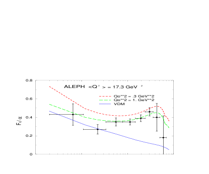
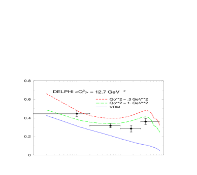
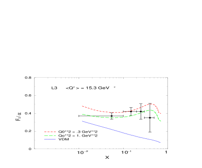
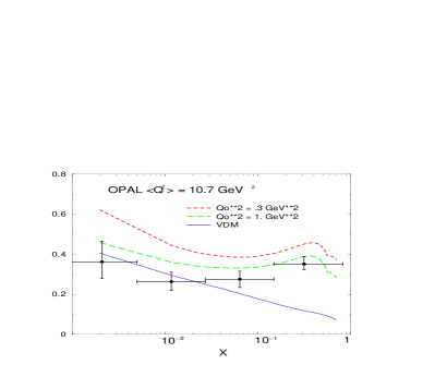
Figure 2: Theory confronted with ALEPH [26], DELPHI [27], L3 [28] and OPAL [29] data in the range 10 GeV${}^{2}\ \raise 1.29167pt\hbox{$<$\kern-7.5pt\raise-4.73611pt\hbox{$\sim$}}\ <\!Q^{2}\!>\ \raise 1.29167pt\hbox{$<$\kern-7.5pt\raise-4.73611pt\hbox{$\sim$}}$ 18 GeV².

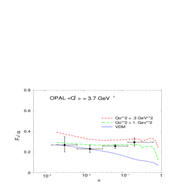
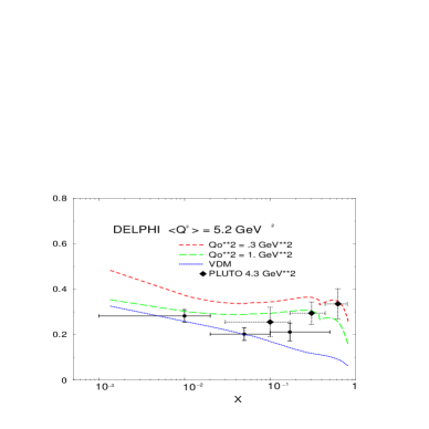
Figure 3: Theory confronted with low-$Q^{2}$ data from OPAL, DELPHI and PLUTO [30].

In Fig. 2, we see that large-$x$ data are poor. Either they have large error bars (ALEPH, L3), or they correspond to large $x$-bins (DELPHI, OPAL). Therefore they cannot accurately constrain $Q_{0}^{2}$ and do not allow us to check the predicted $x$-dependence of $F_{2}^{\gamma}(x,Q^{2})$. On the other hand, all large-$x$ data points ($x\ \raise 1.29167pt\hbox{$>$\kern-7.5pt\raise-4.73611pt\hbox{$\sim$}}\ .2$) favor a value of $Q_{0}^{2}$ close to 1 GeV² ; the choice $Q_{0}^{2}=.3$ GeV² leads to predictions well above the experimental points. This is also true for smaller values of $x$ where the VDM contribution is large. However in this $x$-region we expect a strong correlation between $Q_{0}^{2}$ and $C_{np}$.

The low-$Q^{2}$ data of Fig. 3 lead us to the same conclusion. However whereas the agreement between OPAL data and theory is good, suggesting a slightly smaller contribution of the VDM component, DELPHI data on the contrary suggest a very large suppression, by some 30 %, of the VDM component. It is worth noting that the DELPHI points at $x=.05$ and $x=.17$ are below the corresponding OPAL points, although the $Q^{2}$ value is larger. Other data at low $Q^{2}$ do not clarify the situation. PLUTO data [30] are close to the OPAL points, but the error bars are very large. L3 data [31] ($Q^{2}=5$ GeV², not shown) are noticeably above OPAL data at small-$x$, $x\sim 10^{-2}$, and TPC-2$\gamma$ [32] data at $Q^{2}=5.1$ GeV² (not shown) have large error bars.

In order to determine the values of $Q_{0}^{2}$ and $C_{np}$, we proceed to a best fit of the LEP data displayed in Figs. 2 and 3. The theoretical values are calculated with all parameters kept fixed, except $Q_{0}^{2}$ and $C_{np}$, and they are averaged over the corresponding experimental $x$-bins. For a given value of $Q_{0}^{2}$, we look at the value of $C_{np}$ which minimizes the $\chi^{2}$ value, and we obtain the results shown in Fig. 4 for the ALEPH and DELPHI experiments. At the minimum of the curves, the corresponding values of the non-perturbative normalization are respectively $C_{np}$=.60 and $C_{np}$=1.05.

Figure 4: $\chi^{2}$-values as a function of $Q_{0}^{2}$

We obtain very different shapes of the $\chi^{2}$-curves. In fact, L3 and OPAL data lead to $\chi^{2}$-curves very similar to the one displayed in Fig. 4 for ALEPH. Only DELPHI data lead to a false minimum at $Q_{0}^{2}$=1.5 GeV² and $C_{np}$=1.05; there is no true minimum for $Q_{0}^{2}\geq.2$ GeV². It is easy to find the reason for this behavior. The first point at small-$x$ of DELPHI data is high with respect to the next point. This configuration, associated with small errors, drives the fit to small $Q_{0}^{2}$ and $C_{np}$ values and reproduces the steep slope of $F_{2}^{\gamma}(x,Q^{2})$ at small-$x$. Such an effect is not present in the other sets of data. The small errors of the DELPHI data give an important weight to this experiment in a fit of all the data sets shown in Fig. 2 and 3. Therefore when we perform such a fit, we find (Fig. 5 (left)) a result similar to the DELPHI fit of Fig. 4.

Figure 5: $\chi^{2}$-values of the overall fit. Without modification of the DELPHI errors (left) and with modification (right)

As explained in the beginning of this section, we selected medium and low-$Q^{2}$ LEP data in order to constrain the value of $Q_{0}^{2}$. This led us to consider the LEP1 data from DELPHI. However in the LEP2 data from the same experiment, the small-$x$ behavior observed in the LEP1 data is less marked. The DELPHI collaboration, using different Monte Carlo generators, noticed a strong model dependence of the resulting data on $F_{2}^{\gamma}(x,Q^{2})$. For instance the small-$x$ data at $Q^{2}=19$ GeV² show a sizeable dependence on these generators and moreover, two (over three) of the values obtained for $F_{2}^{\gamma}(x,Q^{2})$ are smaller than the one obtained at LEP1 ($Q^{2}=12.7$ Gev²). Therefore, in order to take this scattering into account, we change the errors in the first $x$-bin of the LEP1 DELPHI preliminary data by a factor two. After this modification, we obtain the $\chi^{2}$-curve shown in Fig. 5 (right). The minimum value of the curve at $Q_{0}^{2}\simeq.7$ GeV² is obtained for $C_{np}\simeq.78$, and the $\chi^{2}$ by degree of freedom is $\chi^{2}_{df}=1.03$.

This result demonstrates the good agreement between our theoretical input (3.8) and LEP data. However, as already discussed, these data do not well constrain the large-$x$ behaviour of $F_{2}^{\gamma}$ and the good $\chi^{2}$ shown in Fig. 5 cannot be seen as a confirmation of our large-$x$ theoretical expression. On the other hand we must note that some LEP data are marginally compatible. This is shown in Fig. 6 in which we display the $\Delta\chi^{2}=1$ contour in the $Q_{0}^{2}$ and $C_{np}$ plane. The best fits to the individual data sets are also exhibited and are scattered outside the contour. For instance the L3 data compared to theory calculated with the overall best fit parameters ($Q_{0}^{2}=.7$, $C_{np}=.78$) lead to $\chi^{2}=4.4$ which must be compared to the value obtained at the L3 best fit point ($.7,1.1$) $\chi^{2}=.85$. For OPAL (10.7) we obtain $\chi^{2}=1.76$ compared to $\chi^{2}=.072$.

Figure 6: The $\Delta\chi^{2}=1$ contour in the $Q_{0}^{2}-C_{np}$ plane with the individual best fits of the LEP data. The DELPHI (12.7) point ($Q_{0}^{2}=1.5$ GeV², $C_{np}=1.05$) is outside the figure and DELPHI (3.7) has no minimum for $Q_{0}^{2}<1.9$ GeV².

In order to partially take into account this scattering, we provide three parametrizations compatible with the contour of Fig. 6, corresponding to three different values of $Q_{0}^{2}$ : $Q_{0}^{2}=.34$ GeV², $Q_{0}^{2}=.70$ GeV² (best-fit parametrization) and $Q_{0}^{2}=.97$ GeV². We use the notation AFG04 $(Q_{0}^{2},C_{np},p_{10})$ and the short-hand notations AFG04_BF = AFG04(.7, .78, 1.9), AFG04_LW = AFG04(.34, .6, 1.9) and AFG04_HG = AFG04(.97, .84, 1.9) for the parametrizations presented in Appendix B.

We would obtain similar results from the world data on $F_{2}^{\gamma}$, but with a larger scattering of the various experiments. This can be observed from Figs. 7, 8 and 9 in which we compare our best fit prediction with these data [26]-[46]. Whereas the overall agreement is good, some data are clearly outside the general trend represented by the best fit. Therefore a general fit leading to a single parametrization has not a clear meaning. It is why we prefer to “frame” the data by several parametrizations, as we did after the analysis of recent low and medium $Q^{2}$ data sensitive to $Q_{0}^{2}$ and $C_{np}$.

Figure 7: Comparison between the best fit structure function and the world data with 3.7 GeV${}^{2}<\ \ <\!Q^{2}\!>\ \ <11$ GeV².

Figure 8: Comparison between the best fit structure function and the world data with 11 GeV${}^{2}<\ <\!Q^{2}\!>\ <29$ GeV².

Figure 9: Comparison between the best fit structure function and the world data with 29 GeV${}^{2}<\ <\!Q^{2}\!>\ <700$ GeV².

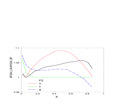
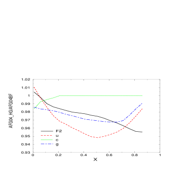
Figure 10: The Low-$Q_{0}^{2}$ (left) and the High-$Q_{0}^{2}$ (right) parametrizations compared to the best-fit parametrization.

Let us now compare, in Fig. 10, the Low-$Q_{0}^{2}$ and High-$Q_{0}^{2}$ AFG04 parametrizations to the best-fit parametrization. Let us consider the figure at the left. At small values of $x$ where the non-perturbative component is large, the ratio partly reflects the values of $C_{np}$ used in AFG04_BF and AFG04_LW. At very small values of $x$, the perturbative contribution becomes dominant and the ratio reflects the effect of the $Q^{2}$-evolution which is larger for AFG04_LW. At $x\sim.5$, the non-perturbative contribution is smaller and the ratio also reflects the effect of the $Q^{2}$-evolution of the perturbative component. For large-$x$ values, the $u$-quark distribution contains a term proportionnal to $\ln(1-x)$. Adding the contribution from $k_{q}^{(1)}$ (2.12) to the $C_{\gamma,c}^{f}$ contribution (3.7), we obtain a term proportionnal to $\displaystyle{{\ln n\over n}}(1+(\alpha_{s}(Q^{2})/\alpha_{s}(Q_{0}^{2}))^{-2P_{qq}^{(0)}/\beta_{0}})$ which is large for a small evolution $(P_{qq}^{(0)}(n)$ being negative at large $n$). The $u$-quark ratio reflects this behavior. Finally we note that the variations in the distribution functions never exceed 10 %.

We end this section by a few words on other NLO parametrizations. Let us start with the AFG one. In fact the AFG parametrization is very close to the parametrization AFG04(.5, 1., 1.9). The only differences come from the values of $\Lambda_{\overline{MS}}^{(4)}$ (300 MeV in AFG04 and 200 MeV in AFG) and from the absence of bottom quark distribution in AFG. The comparison is done at $Q^{2}=50$ GeV², a scale which is in the range of those used in large-$p_{\bot}$ photoproduction. The ratio of the best-fit distribution AFG04_BF to the AFG distribution is displayed in Fig. 11. The smaller normalization of the non-perturbative component of AFG04_BF compared to the one used in AFG explains the pattern at small-$x$ values. However, at very small values of $x$, the inhomogeneous kernels $k_{q}^{(1)}$ and $k_{g}^{(1)}$ (2.4 and 2.5) have a singular behavior ($k_{q}^{(1)}\sim\ln^{2}x$ and $k_{g}^{(1)}\sim{1\over x}$) and the behavior of the perturbative gluon and sea components reflect a faster evolution of AFG04 with $Q^{2}$ due to the larger value of $\Lambda_{\overline{MS}}$. At large-$x$ values the perturbative contributions are important and the ratio of the $u$-quark distribution is close to the ratio $r=\alpha_{s}(AFG)/\alpha_{s}(AFG04)$ at $Q^{2}=50.$ GeV², namely $r\sim.9$. The difference in the predictions for $F_{2}^{\gamma}$ are illustrated in the figure on the right. It is not very large, and could be distinguishable only at large values of $x$ where data are poor. Comparisons between AFG04_BF and AFG predictions are given for OPAL (3.7), OPAL (10.7) and ALEPH (67.2) in Figs. 7 and 9.

A comparison with the GRS [10] parametrization can also be performed on the basis of Figs. 7 and 8. In the second reference of [10], a comparison is made between OPAL data and the GRS predictions which can hardly be distinguished from our best fit curves at $Q^{2}=3.7$, 10.7 and 17.8 GeV². However note that the large-$x$ behaviors of $F_{2}^{\gamma}$ (outside the data range) are quite different between the GRS and the AFG04_BF parametrizations. This behavior comes from the different factorization schemes used ($\overline{MS}$ versus $DIS_{\gamma}$ [10]), associated with different non perturbative inputs (compare (3.8) and (3.10)).

In a recent publication, the authors of ref. [11] proposed new 5 flavor NLO parametrizations and did detailed comparisons with world data, and other (AFG and GRS) parametrizations. On the basis of Figs. 7, 8 and 9, and of similar figures in ref. [11], we can easily observe several differences between the parametrizations. At small $x$ ($x\ \raise 1.29167pt\hbox{$<$\kern-7.5pt\raise-4.73611pt\hbox{$\sim$}}\ 10^{-2}$) and for $Q^{2}\ \raise 1.29167pt\hbox{$>$\kern-7.5pt\raise-4.73611pt\hbox{$\sim$}}\ 5$ GeV² the parametrizations of ref. [11] are higher than AFG04_BF (which is very close to GRS). This trend increases with $Q^{2}$. At medium $x$ in the charm threshold region and at larger values of $x$ ($x\ \raise 1.29167pt\hbox{$>$\kern-7.5pt\raise-4.73611pt\hbox{$\sim$}}\ .6$), the differences between AFG04_BF, and the FFNS${}_{\rm CJK}1$ and CJK NLO parametrizations of ref. [11] are also noteworthy. Here also the origin of this difference is the different non perturbative inputs associated with the $\overline{MS}$ scheme (expression (3.8)) and the $DIS_{\gamma}$ scheme used in ref. [11]. In all cases data are not accurate enough to enable to distinguish between the models.

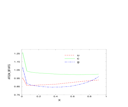
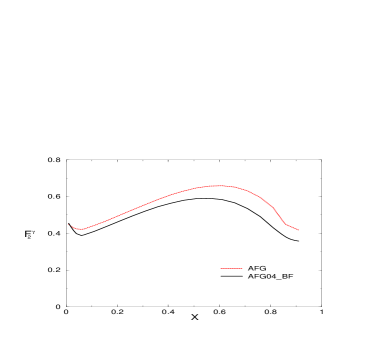
Figure 11: The ratios AFG04_BF/AFG at $Q^{2}=50.$ GeV²(left) and the structure functions $F_{2}^{\gamma}(x,Q^{2})$ (right).

6 The gluon content of the photon

In this section we study other possible options for the parametrization of the parton distributions in the photon. First we study a modification of the sea quark distributions. Then we investigate the effect of changing the normalization of the sea quark and gluon distributions. And finally we modify the large-$x$ shape of the gluon distribution. As we shall see, these modifications are poorly constrained by $F_{2}^{\gamma}$ data, but some of them could be visible in photoproduction experiments.

The small-$x$ behavior of the sea quark distribution (4.4b) that we used until now is less steep than those of some recent parton distributions in the proton [48, 49, 50]. For instance we have $x(\overline{u}+\overline{d})\sim.061/x^{.3}$ at $x<10^{-3}$ for the CTEQ6M distribution at $Q_{0}^{2}=1.69$ GeV². In order to explore the effect of such a steep behavior, we modify our sea distribution (4.4b), while keeping fixed the momentum carried by the sea quarks ($\int_{0}^{1}dx\ x\ q_{sea}^{\pi}(x,Q_{0}^{2}=2$ GeV${}^{2})=.14$)

$$xq_{sea}^{\pi}=.48(1-x)^{7.5}/x^{.3}\ .$$ (6.1)

This ansatz corresponds to quite a large sea at small-$x$, larger by more than a factor 2 than the corresponding CTEQ6M parametrization for the proton. Therefore (6.1) must be considered as an extreme parametrization.

The resulting $\chi^{2}$ is less satisfactory than the one obtained in the preceding section. With the exception of DELPHI, the individual $\chi^{2}$ deteriorate. The total best fit now corresponds to $\chi^{2}=34.3$ (without DELPHI-errors modification), close to the value of section 5. If we modify the errors, we obtain $\chi^{2}=31.4$, instead of 25.8 in section 5. From these results, we see that there is no compelling reason to modify the small-$x$ behavior of the sea distributions we used in the preceding section.

Figure 12: Correlation between the parameters $C_{mom}$ and $C_{np}$. The numbers are the $\chi^{2}$-values.

Let us now study the effects of the parameter $C_{mom}$ which modifies the normalization of the sea quark and gluon distributions according to (4.7a, 4.7b) (at small-$x$ values, sea quark and gluon distributions are strongly coupled and we modify their normalizations by the same parameter $C_{mom}$). If we keep $Q_{0}^{2}$ and $C_{np}$ at the best fit values established in section 5, $C_{mom}$ is quite constrained by $F_{2}^{\gamma}$ data and the $\chi^{2}$-value varies by less than one unit if we stay in the domain $.92\ \raise 1.29167pt\hbox{$<$\kern-7.5pt\raise-4.73611pt\hbox{$\sim$}}\ C_{mom}\ \raise 1.29167pt\hbox{$<$\kern-7.5pt\raise-4.73611pt\hbox{$\sim$}}\ 1.08$. However it is clear that we can partially compensate the $C_{mom}$ variations by also varying $C_{np}$. Keeping $Q_{0}^{2}=.7$ GeV², we first observe a strong correlation between $C_{np}$ and $C_{mom}$ (Fig. 12). By playing with the values of $C_{mom}$ and $C_{np}$, for instance, we can enhance the importance of the valence compared to the sea quark. But it is unlikely that photoproduction experiment could better constrain $C_{np}$ and $C_{mom}$ and we do not pursue this study in detail.

Figure 13: $\chi^{2}$ variation as a function of the gluon parameter $p_{10}$.

Finally we consider the modification of the gluon distribution and we vary the parameter $p_{10}$ of expression (4.4c). As expected $F_{2}^{\gamma}$ is not sensitive to the gluon distribution and LEP data do not constrain the value of $p_{10}$. We display in Fig. 13 the dependence of the $\chi^{2}$ on $p_{10}$ which is weak ($Q_{0}^{2}$ and $C_{np}$ being fixed at the best fit values). In a large range in $p_{10}$, $\chi^{2}$ varies by less than one unit. In Fig. 14 we show the behaviour of the distributions obtained with $p_{10}=1.0$ (hard gluon) and $p_{10}=4.0$ (soft gluon) at $Q^{2}=50.$ GeV², the other parameters being kept fixed at the best-fit values. The behavior at small values of $x$ is due to the normalization factor $C_{g}$ (4.4c) ; at large values of $x$ the non-perturbative inputs vanish and the ratios go to one.

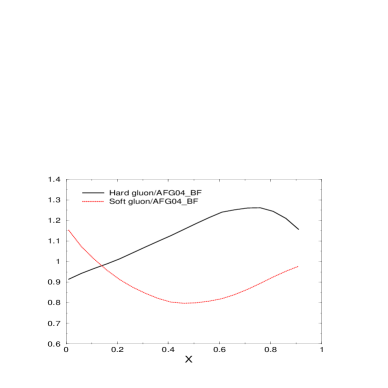
Figure 14: Ratios of the gluon distributions with $p_{10}=4.0$ (soft gluon) and $p_{10}=1.0$ (hard gluon) to the best-fit gluon at $Q^{2}=50.$ GeV².

On the other hand photoproduction reactions [51] are sensitive to the gluon distribution since an initial gluon can interact with a parton from the initial proton producing two large-$p_{\bot}$ jets in the final state. Jet production in photon-photon collisions is also a reaction allowing to observe the gluon distribution in the range $0<x\ \raise 1.29167pt\hbox{$<$\kern-7.5pt\raise-4.73611pt\hbox{$\sim$}}\ .4$ [52]. A particularly interesting reaction is the photoproduction of large-$p_{\bot}$ photon and jet, which has been studied in ref. [7] in detail. The interest of this reaction comes from the fact that the scale dependence of the cross section is well under control, and therefore, the theoretical predictions are reliable. We quote here one result of this paper, referring the interested reader to the original publication [7]. Fig. 15 displays the cross sections $d\sigma/dx_{LL}$, where $x_{LL}=p_{\bot}^{\gamma}$ ($e^{-\eta_{\gamma}}+e^{-\eta_{jet}})/2E_{\gamma}$, for various cuts on the rapidities $\eta^{\gamma}$ and $\eta^{jet}$ ($E_{\gamma}$ is the energy of the initial photon). In the forward region where the rapidities $\eta^{\gamma}$, $\eta^{jet}$ are large, the cross section is dominated by the resolved contribution. For some cuts, half of the cross section is due to the gluon distribution in the photon. But the observable range in $x$ is small ($x\ \raise 1.29167pt\hbox{$<$\kern-7.5pt\raise-4.73611pt\hbox{$\sim$}}\ .2$) and the cross sections fairly small. However this type of data could be used to constrain the poorly known $G^{\gamma}(x,Q^{2})$.

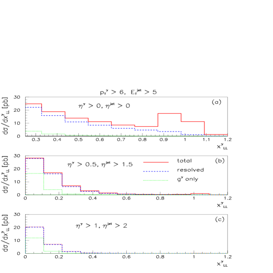
Figure 15: The enhancement of the gluon contribution to the reaction $\gamma+p\to\gamma+jet+X$ due to cuts on the rapidities $\eta_{\gamma}$ and $\eta_{jet}$.

7 Conclusions

We have proposed a new set of next-to-leading order parton distributions for real photons. We work in the $\overline{MS}$ scheme with a variable number of massless flavors, keeping however the massive correction terms for charm and beauty quarks, in the direct contribution to the ${\cal{F}}_{2}^{\gamma}$ structure function. The perturbative contribution is assumed to vanish below a $Q_{0}^{2}$ value and a VDM type parametrisation is used for the non-perturbative input at this value. We give a detailed discussion on how to isolate the scheme invariant piece of the structure function to which the physical VDM input should be applied. The distributions are set up such that various input parameters can be easily changed: these are the value of $Q_{0}^{2}$, the overall normalisation of the non-perturbative input and the x-dependence of the gluon which is poorly constrained by the photon structure function data. Using the LEP data, an attempt to decorrelate the perturbative contribution, controlled by $Q_{0}^{2}$, from the non-perturbative one is made. It turns out that the error bars are too large to determine unambiguously the value of $Q_{0}^{2}$. A best fit to low and medium-$Q^{2}$ LEP data is then done which is also shown to yield a good agreement with the world data. A large dispersion in the value of the best fit parameters is observed when a minimum $\chi^{2}$ fit is performed for each set of LEP data independently. We therefore propose several sets of parton distributions to “frame” the data. Since the gluon distribution cannot be constrained from the deep inelastic data, we suggest to consider the photoproduction of photons, hadrons or jets at large transverse momentum.

Appendix A - Appendix A

In this appendix, we give a derivation of expression (3.7). We start from the reaction in which the target photon, instead of being real, has a small virtuality $p^{2}$ $(-p^{2}\equiv P^{2}\ll Q^{2})$, but large enough for the perturbative approach to be valid. This allows us to study the structure of the HO corrections to ${\cal F}_{2}^{\gamma}$ and to understand how to take the real photon limit $p^{2}\to 0$. The transverse structure function ${\cal F}_{2}^{T}(Q^{2},P^{2},n)$ (transverse with respect to the polarisation of the target photon) can be written

$${\cal F}_{2}^{T}(Q^{2},P^{2},n)=\sum_{f}e_{f}^{2}\ C_{q}(n)\ q_{f}^{NS}(Q^{2},P^{2},n)+C_{\gamma}^{NS}(n)$$ (A.1)

where, for simplicity, we only consider the Non Singlet contribution.

This expression is obtained in resumming all the $\ln(Q^{2}/P^{2})$ in the quark distribution $q_{f}^{NS}(Q^{2},P^{2},n)$, whereas $C_{q}(n)$ and $C_{\gamma}^{NS}(n)$ are expansions in power of $\alpha_{s}(Q^{2})$. This procedure defines a factorization scheme called “Virtual Factorization Scheme” in ref. [53]. In this scheme the Wilson coefficient $C_{q}(n)$ and the direct term $C_{\gamma}^{NS}(n)$ are known since the work of Uematsu and Walsh [54].

The quark distribution is a solution of eq. (2.2) (we drop the index NS and the moment variable $n$)

$$q_{f}(Q^{2},P^{2})=\sigma_{f}\int_{\alpha_{s}(P^{2})}^{\alpha_{s}(Q^{2})}{d\lambda\over\beta(\lambda)}\ k_{q}(\lambda)\ e^{\int_{\lambda}^{\alpha_{s}(Q^{2})}{d\lambda^{\prime}\over\beta(\lambda^{\prime})}\ P_{qq}(\lambda)}\ .$$ (A.2)

To simplify the notation further, we consider one quark species and drop the charge factors which are present in $\sigma_{f}k_{q}(\lambda)$ of (A.2) (that we shall note $k(\lambda)$) and in $C_{\gamma}^{NS}$. With this convention, the direct term is written [54]

$$C_{\gamma}(x) = {\alpha\over 2\pi}\ 6\Big{\{}\left[(x^{2}+(1-x)^{2})\ln{1\over x}+2x(1-x)-1\right]$$ (A.3)

$$+\left(x^{2}+(1-x)^{2}\right)\ln{1\over x}+6x(1-x)-1\Big{\}}\ .$$

It is worth noting the following points. First $C_{\gamma}(x)$ is scheme dependent and different from the $\overline{\rm MS}$ expression (2.7). However it is easy to move from the Virtual Scheme to the $\overline{\rm MS}$ scheme by keeping in mind that expression (2.14) must be scheme invariant, which leads to

$${\alpha\over 2\pi}\left({k^{(1)^{\overline{MS}}}(n)\over P_{qq}^{(0)}(n)}-{k^{(1)}(n)\over P_{qq}^{(0)}(n)}\right)=C_{\gamma}^{\overline{MS}}(n)-C_{\gamma}(n)\equiv\Delta C(n)$$ (A.4)

where, from (2.7) and (A.3)

$$\Delta C(x)={\alpha\over 2\pi}6\left\{\left(x^{2}+(1-x)^{2}\right)\ln\ x(1-x)+1\right\}$$ (A.5)

in the $x$-space.

Second, the direct terms $C_{\gamma}$ are target dependent and depend on the regularization used to avoid a collinear divergence in the calculation of the box diagram. For instance, in dimensional regularization, the target dependent part has been calculated in section 3, and is given by $C_{\gamma,c}^{f}$ (3.4) (in which $e_{f}^{4}$ is dropped). For a virtual photon, we obtain the first line of (A.3) [53], whereas the second line is universal and equal to the equivalent $\overline{\rm MS}$ expression. Therefore we can write in general

$$C_{\gamma}(x)=C_{\gamma}^{col}(x)+C_{\gamma}^{U}(x)\ .$$ (A.6)

With the notation “col”, we indicate that the target dependent part of $C_{\gamma}$ comes from the lower limit of the integration over $k^{2}$ (cf. expression 3.2 and 3.3). A similar decomposition exists for $k^{(1)}$

$$k^{(1)}=k^{(1)^{col}}+k^{(1)^{U}}$$ (A.7)

because the target dependent terms, which are present in $C_{\gamma}(x)$, also appear in the course of the calculation of $k^{(1)}$ under the form $C_{\gamma}^{col}(n)$ $P_{qq}^{(0)}(n)$ (this point has been discussed in detail in ref. [53]). Therefore the combination

$$-{\alpha\over 2\pi}\ {k^{(1)}(n)\over P_{qq}^{(0)}(n)}+C_{\gamma}(n)=-{\alpha\over 2\pi}\ {k^{(1)^{U}}(n)\over P_{qq}^{(0)}(n)}+C_{\gamma}^{U}(n)$$ (A.8)

and consequently ${\cal F}_{2}(Q^{2},P^{2},n)$ (when $Q^{2}$ is very large) does not depend on the details of the target.

We are now ready to study the limit $P^{2}\to 0$ of expression (A.2). With this aim in view, we introduce an intermediate scale $Q_{0}^{2}$ which allows us to isolate the $P^{2}$-dependent part of (A.2)

$$q(Q^{2},P^{2})=q(Q^{2},Q_{0}^{2})+\int_{\alpha_{s}(P^{2})}^{\alpha_{s}(Q_{0}^{2})}{d\lambda\over\beta(\lambda)}\ k({\lambda})\ e^{\int_{\lambda}^{\alpha_{s}(Q^{2})}{d\lambda^{\prime}\over\beta(\lambda^{\prime})}P_{qq}(\lambda^{\prime})}\ ,$$ (A.9)

where $q(Q^{2},Q_{0}^{2})$ is given by (A.2) in which $P^{2}$ is replaced by $Q_{0}^{2}$ (in section 3, $Q_{0}^{2}$ is the limit between the perturbative and the non-perturbative domains). Using the notation

$$k(\lambda)={\alpha\over 2\pi}\left\{k^{(0)}+{\lambda\over 2\pi}\ k^{(1)^{U}}+{\lambda\over 2\pi}\ k^{(1)^{col}}\right\}=k^{U}(\lambda)+{\alpha\over 2\pi}\ {\lambda\over 2\pi}\ k^{(1)^{col}}$$ (A.10)

we rewrite the integral in (A.9)

$$\left\{\int_{P^{2}}^{Q_{0}^{2}}{dk^{2}\over k^{2}}k^{U}(\lambda)\ e^{\int_{k^{2}}^{Q_{0}^{2}}{dk^{\prime 2}\over k^{\prime 2}}P_{qq}}-{\alpha\over 2\pi}\ {k^{(1)^{col}}\over P_{qq}^{(0)}}\left(1-\left({\alpha_{s}(Q_{0}^{2})\over\alpha_{s}(P^{2})}\right)^{-2{P_{qq}^{(0)}\over\beta_{0}}}\right)\right\}\cdot e^{\int_{\alpha(Q_{0}^{2})}^{\alpha(Q^{2})}{d\lambda^{\prime}\over\beta(\lambda^{\prime})}\ P_{qq}(\lambda^{\prime})}\ .$$ (A.11)

After extracting from (A.11) the $P^{2}$-independent, but target dependent term $k^{(1)^{col}}/P_{qq}^{(0)}$, we define

$$H(Q_{0}^{2},P^{2})=\int_{P^{2}}^{Q_{0}^{2}}{dk^{2}\over k^{2}}\ k^{U}\ e^{\int_{k^{2}}^{Q_{0}^{2}}{dk^{\prime 2}\over k^{\prime 2}}P_{qq}}+{\alpha\over 2\pi}\ {k^{(1)^{col}}\over P_{qq}^{(0)}}\left({\alpha_{s}(Q_{0}^{2})\over\alpha_{s}(P^{2})}\right)^{-2{P_{qq}^{(0)}\over\beta_{0}}}$$ (A.12)

and rewrite ${\cal F}^{T}_{2}$ as

$${\cal F}_{2}^{T}(Q^{2},P^{2},n)=C_{q}\ q(Q^{2},Q_{0}^{2})+C_{q}\left[H(Q_{0},P^{2})-C_{\gamma}^{col}\right]e^{\int_{\alpha_{s}(Q_{0}^{2})}^{\alpha_{s}(Q^{2})}{d\lambda\over\beta(\lambda)}P_{qq}}+C_{\gamma}^{U}+C_{\gamma}^{col}\ ,$$ (A.13)

because $C_{\gamma}^{col}={\alpha\over 2\pi}{k^{(1)^{col}}\over P_{qq}^{(0)}}$. Let us now consider the limit $P^{2}\to 0$ with $Q_{0}^{2}$ being the scale below which the perturbative approach has no meaning. As a consequence, the perturbative expression (A.12) of $H(Q_{0}^{2},P^{2})$ is no longer valid and we can only say that $H(Q_{0}^{2},P^{2})$ contains all the non-perturbative contributions needed to define ${\cal F}_{2}^{\gamma}$ in the real limit. Now we recognize in (A.13) the structure of the input proposed in formula (3.7) if we identify $H(Q_{0}^{2})=\displaystyle{\lim_{P^{2}\to 0}}H(Q_{0}^{2},P^{2})$ to $q^{NP}(Q_{0}^{2})+\overline{q}^{NP}(Q_{0}^{2})$.

Expression (A.13) has been established in the virtual factorization scheme. But we can easily obtain a similar expression in the $\overline{\rm MS}$ scheme by writing $k^{(1)}=k^{(1)^{\overline{MS}}}+\Delta k^{(1)}$ in the expression (A.2) for $q(Q^{2},Q_{0}^{2})$. This change generates a $\overline{\rm MS}$ distribution $q^{\overline{MS}}(Q^{2},Q_{0}^{2})$ and a term (cf. (2.12))

$$-{\Delta k^{(1)}\over P_{qq}^{(0)}}\left(1-\left({\alpha_{s}(Q^{2})\over\alpha_{s}(Q_{0}^{2})}\right)^{-2P_{qq}^{(0)}/\beta_{0}}\right)$$ (A.14)

which is combined with $C_{\gamma}^{col}\left(1-\left({\alpha_{s}(Q^{2})\over\alpha_{s}(Q_{0}^{2})}\right)^{-2P_{qq}^{(0)}/\beta_{0}}\right)$ of (A.13) to give

$$C_{\gamma}^{col,\overline{MS}}\left(1-\left({\alpha_{s}(Q^{2})\over\alpha_{s}(Q_{0}^{2})}\right)^{-2P_{qq}^{(0)}/\beta_{0}}\right)$$

so that (A.13) can be written in terms of $\overline{MS}$ perturbative expressions, together with a non-perturbative contribution $H(Q_{0}^{2})$ which remains invariant under this change.

Appendix B - Appendix B

The parametrizations discussed in this paper are available in the form of a FORTRAN code allowing the users to select the parton distributions they are interested in. The conventions we use are described in table 1 which displays abbreviations of the general notation AFG04($Q_{0}^{2},C_{np},p_{10}$).

	$Q_{0}^{2}=.34$ GeV2	$Q_{0}^{2}=.70$ GeV2	$Q_{0}^{2}=.97$ GeV2
$p_{10}=1.0$		AFG04_BF_1.0
(hard gluon)		($C_{np}=.78$)
$p_{10}=1.9$	AFG04_LW	AFG04_BF	AFG04_HG
(default)	($C_{np}=.60$)	($C_{np}=.78$)	($C_{np}=.84$)
$p_{10}=4.0$		AFG04_BF_4.0
(soft gluon)		($C_{np}=.78$)

Table 1

The values of $C_{np}$ indicated in brackets are the default values ; the users can choose other values (after carefully reading section 5). These parametrizations can be downloaded from the site http://www.lapp.in2p3.fr/lapth/PHOX_FAMILY/main.html.

References

- [1] E. Witten, Nucl. Phys. B120, 189 (1977).
-
[2]
H. Kolanoski, Springer Tract in Modern Physics 105, 187 (1984) ;
Ch. Berger and W. Wagner, Phys. Rep. C146, 1 (1987). - [3] R. Nisius, Phys. Rep. 332, 165 (2000).
- [4] M. Krawczyk, M. Staszel and A. Zembrzuski, Phys. Rep. 345, 265 (2001).
- [5] M. Klasen, Rev. Mod. Phys. 74, 1221 (2002).
- [6] P. Aurenche, M. Fontannaz, J. Ph. Guillet, Z. Phys. C64, 621 (1994).
- [7] M. Fontannaz and G. Heinrich, Eur. Phys. J. C34, 191 (2004).
- [8] H1 Collaboration, C. Adloff et al., hep-ex/0302034.
- [9] P. Aurenche et al., Phys. Lett. B233, 517 (1989).
- [10] M. Glück, E. Reya and I. Schienbein, Phys. Rev. D60, 054019 (1999), Erratum-ibid. D62, 019902 (2000) ; Phys. Rev. D64, 01750 (2001).
- [11] F. Cornet, P. Jankowski, M. Krawczyk, Phys. Rev. D70, 093004 (2004).
- [12] R. De Witt et al., Phys. Rev. D19, 2046 (1979) ; (E) 20, 1751 (1979).
- [13] E. G. Floratos, D. A. Ross, C. T. Sachrajda, Nucl. Phys. B129, 66 (1977) ; E B139, 545 (1978) ; Nucl. Phys. B152, 493 (1979).
-
[14]
G. Curci, W. Furmanski, R. Petronzio, Nucl. Phys.
B175, 27 (1980).
W. Furmanski, R. Petronzio, Phys. Lett. 97B, 437 (1980). - [15] M. Fontannaz and E. Pilon, Phys. Rev. D45, 382 (1992).
- [16] M. Glück, E. Reya and A. Vogt, Phys. Rev. D45, 3986 (1992).
- [17] NLO FORTRAN codes for large- photoproduction reactions can be downloaded from http://www.lapp.in2p3.fr/lapth/PHOX_FAMILY/main.html.
- [18] E. B. Zijlstra and W. L. van Neerven, Nucl. Phys. B383, 525 (1992).
- [19] S. Moch, J. A. M. Vermaseren, A. Vogt, Nucl. Phys. B621, 413 (2002).
-
[20]
S. Moch, J. A. M. Vermaseren, A. Vogt, Nucl. Phys.
B688, 101 (2004).
A. Vogt, S. Moch, J. A. M. Vermaseren, Nucl. Phys. B691, 129 (2004). -
[21]
W. A. Bardeen, A. J. Buras, D. W. Duke and T. Muta,
Phys. Rev. D18, 3998 (1978).
G. Altarelli, R. K. Ellis and G. Martinelli, Nucl. Phys. B157, 461 (1979). - [22] W. A. Bardeen, A. J. Buras, Phys. Rev. D20, 166 (1979) ; D21, 2041 (1980)E.
- [23] M. Glück, E. Reya and A. Vogt, Phys. Rev. D46, 1973 (1992).
-
[24]
E. Witten, Nucl. Phys. B104, 445 (1976) ;
C. T. Hill and G. C. Ross, Nucl. Phys. B148, 373 (1979) ;
M. Glück and E. Reya, Phys. Lett. B83, 98 (1979). - [25] S. Albino, M. Klasen and S. Söldner-Rembold, Phys. Rev. Lett. 89, 122004 (2002).
- [26] ALEPH Collaboration, A. Heister et al., Eur. Phys. J. C30, 145 (2003).
- [27] DELPHI Collaboration, preprint DELPHI 2003-025 CONF 645, contributed paper for EPS 2003 (Aachen) and LP 2003 (FNAL).
- [28] L3 Collaboration, M. Acciarri et al., Phys. Lett. B447, 147 (1999).
- [29] OPAL Collaboration, G. Abbienchi et al., Eur. Phys. J. C18, 15 (2000).
- [30] PLUTO Collaboration, Ch. Berger et al., Phys. Lett. B142, 111 (1984).
- [31] L3 Collaboration, M. Acciarri et al., Phys. Lett. B436, 403 (1998).
- [32] TPC-2 Collaboration, H. Aihara et al., Z. Phys. C34, 1 (1987).
- [33] L3 Collaboration, M. Acciarri et al., Phys. Lett. B483, 373 (2000).
- [34] AMY Collaboration, Sasaki et al., Phys. Lett. 252B, 491 (1990).
- [35] AMY Collaboration, Sahu et al., Phys. Lett. 346B, 208 (1995).
- [36] AMY Collaboration, Kojima et al., Phys. Lett. B400, 395 (1997).
- [37] DELPHI Collaboration, Abreu et al., Zeit. Phys. C69, 223 (1996).
- [38] JADE Collaboration, Bartel et al., Zeit. Phys. C24, 231 (1984) ; Phys. Lett. B121, 203 (1983).
- [39] OPAL Collaboration, Akers et al., Zeit. Phys. C61, 199 (1994).
- [40] OPAL Collaboration, Ackerstaff et al., Zeit. Phys. C74, 33 (1997).
- [41] OPAL Collaboration, Ackerstaff et al., Phys. Lett. B411, 387 (1997).
- [42] OPAL Collaboration, Ackerstaff et al., Phys. Lett. B412, 225 (1997).
- [43] OPAL Collaboration, Abbiendi et al., Phys. Lett. B533, 207 (2002).
- [44] PLUTO Collaboration, Ch. Berger et al., Nucl. Phys. B281, 365 (1987).
- [45] TASSO Collaboration, Althoff et al., Zeit. Phys. C31, 527 (1986).
- [46] TOPAZ Collaboration, Muramatsu et al., Phys. Lett. 332B, 477 (1994).
- [47] M. Fontannaz, J. Ph. Guillet, G. Heinrich, Eur. Phys. J C26, 209 (2002).
- [48] V. Barone, C. Pascaud, F. Zomer, Eur. Phys. J C12, 243 (2000).
- [49] CTEQ Collaboration, J. Pumplin et al., JHEP 0207, 012 (2002).
- [50] MRST Collaboration, A. D. Martin et al., Eur. Phys. J C23, 73 (2002).
- [51] P. Aurenche, L. Bourhis, M. Fontannaz, J. Ph. Guillet, Eur. Phys. J C17, 413 (2000).
- [52] OPAL Collaboration, G. Abbiendi et al., Eur. Phys. J. C31, 307 (2003).
- [53] M. Fontannaz, Eur. Phys. J. C38, 297 (2004).
- [54] T. Uematsu and T. F. Walsh, Nucl. Phys. B199, 93 (1982).