hep-ph/0503246 IFUP–TH/2005–06

Implications of neutrino data circa 2005

Alessandro Strumia

Dipartimento di Fisica dell’Università di Pisa and INFN

Francesco Vissani

INFN, Laboratori Nazionali del Gran Sasso, Theory Group, I-67010 Assergi (AQ), Italy

Abstract

Adopting the 3 neutrino framework, we present an updated determination of the oscillation parameters. We perform a global analysis and develop simple arguments that give essentially the same result. We also discuss determinations of solar neutrino fluxes, capabilities of future experiments, tests of CPT, implications for neutrino-less double-$\beta$ decay, $\beta$ decay, cosmology.

$$\begin{array}[]{|lrlc|}\hline\cr\hbox{Oscillation parameter}&\lx@intercol\hfil\hbox{central value}\hfil\lx@intercol&\hbox{$99\%$ CL range}\\ \hline\cr\color[rgb]{0.45,0,0}\hbox{solar mass splitting}&\color[rgb]{0.45,0,0}\Delta m^{2}_{12}~{}=&\color[rgb]{0.45,0,0}(8.0\pm 0.3)\,10^{-5}{\rm eV}^{2}&\color[rgb]{0.45,0,0}(7.2\div 8.9)\,10^{-5}{\rm eV}^{2}\\ \color[rgb]{0,0,0.4}\hbox{atmospheric mass splitting~{}}&\color[rgb]{0,0,0.4}|\Delta m^{2}_{23}|~{}=&\color[rgb]{0,0,0.4}~{}(2.5\pm 0.3)\,10^{-3}{\rm eV}^{2}{}&\color[rgb]{0,0,0.4}(1.7\div 3.3)\,10^{-3}{\rm eV}^{2}\\ \color[rgb]{0.45,0,0}\hbox{solar mixing angle}&\color[rgb]{0.45,0,0}\tan^{2}\theta_{12}~{}=&\color[rgb]{0.45,0,0}0.45\pm 0.05&\color[rgb]{0.45,0,0}30^{\circ}<\theta_{12}<38^{\circ}\\ \color[rgb]{0,0,0.4}\hbox{atmospheric mixing angle}&\color[rgb]{0,0,0.4}\sin^{2}2\theta_{23}~{}=&\color[rgb]{0,0,0.4}1.02\pm 0.04&36^{\circ}<\theta_{23}<54^{\circ}\\ \color[rgb]{0,0.6,0.01}\hbox{`CHOOZ' mixing angle}&\color[rgb]{0,0.6,0.01}\sin^{2}2\theta_{13}~{}=&\color[rgb]{0,0.6,0.01}0\pm 0.05&\color[rgb]{0,0.6,0.01}\theta_{13}<10^{\circ}\\ \hline\cr\end{array}$$

$$\begin{array}[]{|ccc|cc|}\hline\cr\hbox{non-oscillation}&\hbox{probed}&\hbox{experimental}&\hbox{$99\%$ CL range}&\hbox{$99\%$ CL range}\\ \hbox{parameter}&\hbox{by}&\hbox{limit at $99\%$ CL}&\hbox{normal hierarchy}&\hbox{inverted hierarchy}\\ \hline\cr\hbox{$ee$-entry of $m$}&\hbox{$0\nu 2\beta$}&m_{ee}<0.38\,h\,{\rm eV}&(1.1\div 4.5)\,{\rm meV}&(12\div 57)\,{\rm meV}\\ \hbox{$(m^{\dagger}m)^{1/2}_{ee}$}&\hbox{$\beta$-decay}&m_{\nu_{e}}<2.0\,{\rm eV}&(4.6\div 10)\,{\rm meV}&(42\div 57)\,{\rm meV}\\ \hbox{$m_{1}+m_{2}+m_{3}$}&\hbox{cosmology}&m_{\rm cosmo}<0.94\,{\rm eV}&(51\div 66)\,{\rm meV}&(83\div 114)\,{\rm meV}\\ \hline\cr\end{array}$$

Table 1: Summary of present information on neutrino masses and mixings from oscillation data (upper rows) and inferences and limits on non-oscillation probes (lower rows) A $99\%$ C.L. range is a $2.58\sigma$ range. Some $0\nu 2\beta$ data are controversial, and $h\sim 1$ parameterizes uncertain nuclear matrix elements.

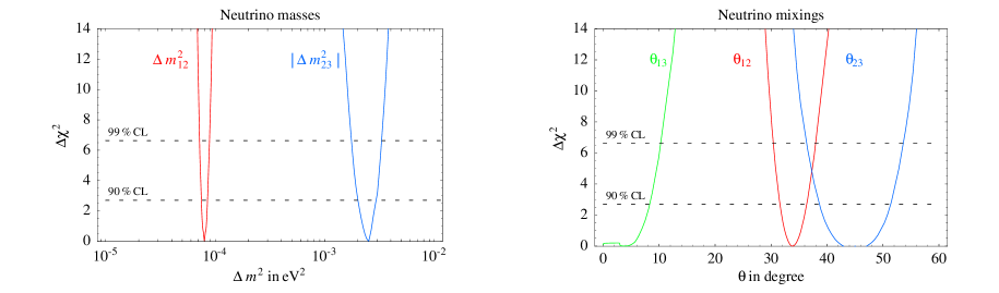
Figure 1: Summary of present information on neutrino masses and mixings from oscillations.

The most plausible extension of the Standard Model that allows to interpret a wealth of neutrino data [1, 2, 3, 4, 5, 6, 7, 8, 9, 10, 11] consists in adding a Majorana mass term for neutrinos,

$$\mathscr{L}=\mathscr{L}_{\rm SM}+\frac{1}{2}({\nu}\cdot m\cdot\nu+\hbox{h.c.})\,\qquad m=V^{*}\cdot\mbox{diag}(m_{1},\ m_{2}\ e^{2i\alpha},\ m_{3}\ e^{2i\beta})\cdot V^{\dagger}.$$ (1)

For normal mass hierarchy we order the neutrino masses $m_{1,2,3}\geq 0$ as $m_{1}<m_{2}<m_{3}$, whereas for inverted mass hierarchy we choose $m_{3}<m_{1}<m_{2}$. The neutrino mixing matrix is

$$V=R_{23}(\theta_{23})\ \mbox{diag}(1,e^{i\phi},1)\ R_{13}(\theta_{13})\ R_{12}(\theta_{12}).$$ (2)

A similar result holds in the case of Dirac masses, with the difference that the number of physical parameters decreases from 9 to 7: the Majorana phases $\alpha$ and $\beta$ can be reabsorbed by field redefinitions.

Data on neutrino oscillations fix $\theta_{12},\theta_{23},\Delta m^{2}_{12}$ and $|\Delta m^{2}_{23}|$ where $\Delta m^{2}_{ij}\equiv m_{j}^{2}-m_{i}^{2}$. As discussed later (sections 1 and 2) our present knowledge of oscillation parameters is approximatively summarized in the upper rows of table 1. The uncertainties are almost Gaussian in the chosen variables; fig. 1 shows the full $\chi^{2}$ functions. Correlations among parameters are ignored because negligible, with the exception that the upper bound on $\theta_{13}$ depends on $|\Delta m^{2}_{23}|$. While $\theta_{12}$ is rather precisely measured, the other 2 mixing angles have large uncertainties. Planned long-baseline oscillation experiments can strongly improve on $\Delta m^{2}_{23}$ and (if $\theta_{13}\,\raise 1.29167pt\hbox{$>$\kern-7.5pt\lower 4.30554pt\hbox{$\sim$}}\,1^{\circ}$) measure $\theta_{13}$, the phase $\phi$, and determine which type of mass hierarchy is realized in nature.

Oscillation experiments, however, are insensitive to the absolute neutrino mass scale (say, the mass of the lightest neutrino) and to the 2 Majorana phases $\alpha$ and $\beta$. Other types of experiments can study some of these quantities and the nature of neutrino masses. They are: $\beta$-decay experiments, that in good approximation probe $m_{\nu_{e}}^{2}\equiv(m\cdot m^{\dagger})_{ee}=\sum_{i}|V_{ei}^{2}|m_{i}^{2}$; neutrino-less double-beta decay ($0\nu 2\beta$) experiments, that probe the absolute value of the Majorana mass $m_{ee}\equiv\sum_{i}V_{ei}^{2}m_{i}$; cosmological observations (Large Scale Structures and anisotropies in the Cosmic Microwave Background), that in good approximation probe $m_{\rm cosmo}\equiv\Omega_{\nu}h^{2}\cdot 93.5{\rm eV}=\sum_{i}m_{i}$. Only neutrinoless double beta decay ($0\nu 2\beta$) probes the Majorana nature of the mass. The values $|m_{ee}|,m_{\nu_{e}},m_{\rm cosmo}$ are unknown, but can be partially inferred from oscillation data. Table 1 shows our results, discussed in section 3, in the limit where the mass of the lightest neutrino is negligible. In the opposite limit neutrinos are quasi-degenerate and $|m_{ee}|,m_{\nu_{e}},m_{\rm cosmo}$ can be arbitrarily large.

From the point of view of 3 massive neutrinos, it is natural to divide in three parts a discussion of the present situation and of the perspectives of improvements, namely:

• Oscillations with ‘solar’ frequency, that tell $\Delta m^{2}_{12}$ and $\theta_{12}$ and give a sub-dominant constraint on $\theta_{13}$. In section 1 we discuss solar and reactor neutrino experiments, showing that the program of measurement of parameters is well under way (if not accomplished), and discussing other interesting related goals.

• Oscillations with ‘atmospheric’ frequency, that tell $\Delta m^{2}_{23}$, $\theta_{23}$ and $\theta_{13}$, are discussed in section 2.

• Non-oscillation experiments, that can tell the absolute neutrino mass. In section 3 we discuss the present status and assess the implications of the existing information on neutrino oscillations for these experiments, particularly for $0\nu 2\beta$. We conclude by commenting on the recent claim of evidence for this transition [12, 13].

We assume the 3 neutrino framework because it is plausible, well defined, restrictive and compatible with data. However it is just an assumption, and before proceeding we recall some alternatives. The most plausible one is the presence of extra light fermions (‘sterile neutrinos’) or bosons, which can manifest in many ways. Going to rather exotic scenarios, Lorentz or CPT invariance (here studied in fig. 3) might be violated in neutrinos, that might have anomalous interactions (gauge couplings, or magnetic moments, or else), might not obey the Pauli principle, etc, etc, etc. Present solar and atmospheric data cannot be explained by these alternatives, which however might be present as sub-leading effects on top of oscillations among active neutrinos, such that our determinations of active oscillation parameters would need model-dependent modifications. The present data do not give any clear indication for extra effects, but contain some anomalous hints. Most notably, the LSND anomaly [14] is not compatible with the 3 neutrino context we assume.

1 Oscillations with solar frequency

A few years ago the solar anomaly rested on global fits that combined solar model predictions with a few measurements of solar neutrino rates. In recent times, the situation changed. As prospected in [15] (written a few years ago, while sub-MeV solar experiments were discussed as a tool for discriminating LMA from LOW, SMA, QVO,…), SNO, KamLAND, Borexino had in any case the capability to identify the true solution of the solar anomaly and make precision measurements of the oscillation parameters. This is where we are now. From the point of view of the determination of the oscillation parameters, solar neutrino experiments are in a more advanced stage than atmospheric experiments, as clear from fig. 1. KamLAND and SNO play the key rôle in the determination for $\Delta m^{2}_{12}$ and $\theta_{12}$ respectively, and almost achieved the $2.5\%$ and $10\%$ accuracy prospected in [15]. In section 1.1 we present a global solar fit, and in section 1.2 we show that it is dominated by very simple and robust inputs. In section 1.3 we extract from data the survival probability of low-energy neutrinos, and use it to study how solar data mildly restrict $\theta_{13}$. In section 1.4 we reassess the interest in proceeding with low-energy solar neutrino experiments. In section 1.5 we discuss how well present solar data determine solar neutrino fluxes and discuss the impact of Borexino. In all cases we extract from simple arguments the main general results, that we compare with ‘exact’ results of global fits performed in specific cases.

1.1 Updated fit of solar and reactor neutrino data

We begin by presenting a global fit of solar and reactor neutrino data assuming oscillations among active neutrinos with negligible $\theta_{13}$. We include

• The final SNO CC, NC, ES rates measured during day and during night without [6] and with [7] salt, that gives enhanced NC sensitivity.

• The Super-Kamiokande ES spectra [5].

• The Gallium rate, $R_{\rm Ga}=(68.1\pm 3.7)\,{\rm SNU}$, obtained averaging the most recent SAGE data with the final Gallex and GNO data [2, 3, 4].

• The Chlorine rate [1], $R_{\rm Cl}=(2.56\pm 0.23)\,{\rm SNU}$.

• The KamLAND reactor anti-neutrino data with prompt energy higher than $2.6\,{\rm MeV}$ [8].

Solar model predictions and uncertainties [16] are revised including the recent measurement of the ¹⁴N$(p,\gamma)^{15}$O nuclear cross section [17], which reduces the predicted CNO fluxes by roughly $50\%$.

The result of our oscillation fit is shown in fig. 2a, where the best fit point is marked with a dot. The $1\sigma$ (i.e. $68\%$ C.L.) and the $99\%$ C.L. (i.e. $2.58\sigma$) ranges for the single parameters (1 dof) are summarized in table 1. The total evidence for an effect is now about 12$\sigma$ in solar $\nu$ data and about 6$\sigma$ in KamLAND $\bar{\nu}$ data. Fig. 2a also shows separately the fit of solar data (dashed red contours) and the fit of KamLAND data (dotted blue contours).

We note in passing that, according to the Pearson $\chi^{2}$ goodness-of-fit (gof) employed by many old global analyses, today the LOW solution (with $\Delta m^{2}_{12}\approx 10^{-7}{\rm eV}^{2}$) still has a good gof. This does not mean that LOW is compatible with data, but happens because the Pearson test is not a statistically powerful gof test when $\hbox{dof}\gg 1$ [18]: global fits of solar data input roughly $100$ experimental inputs. As we now discuss, the output depend almost only on a few pieces of data.

      

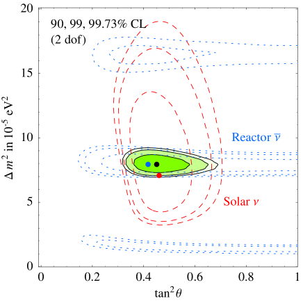
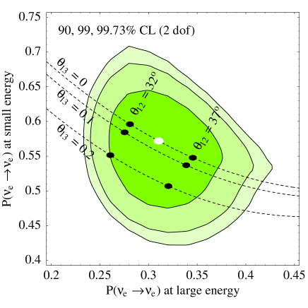
Figure 2: Best-fit regions at $90,~{}99$ and $99.73\%$ CL. Fig. 2a assumes CPT invariance and combines solar $\nu$ data (dashed red contours) with reactor $\bar{\nu}$ data (dotted blue contours). In fig. 2a we show how data determine the high- and low-energy limits of $P(\nu_{e}\to\nu_{e})$, as precisely described in the text,

      

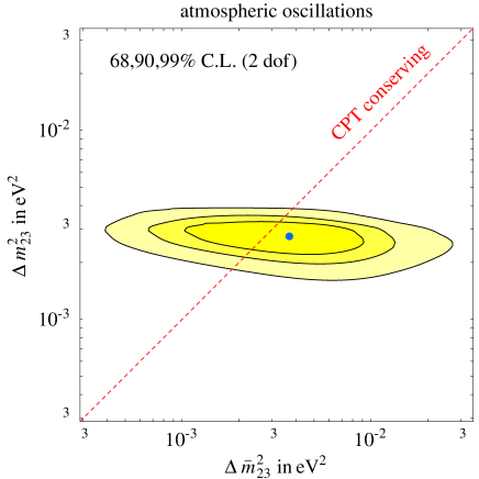
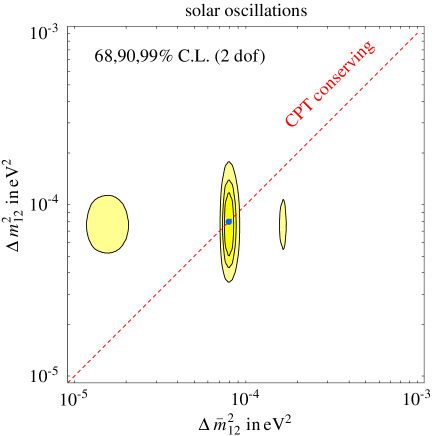
Figure 3: Test of CPT-violating neutrino masses. We show the separate fit for $\Delta m^{2}$ in neutrinos and $\Delta\bar{m}^{2}$ in anti-neutrinos, marginalized with respect to the mixing angles $\theta_{12}$ and $\theta_{23}$. The atmospheric fit includes data from SK, K2K, Macro. The solar fit includes data from SNO, SK, Gallex, Sage, Homestake, KamLAND. These plots update the original results in fig.s 5 and 6 of [19]

1.2 The meaning of ‘global fits’

Our results are based on a careful global fit. We now point out how a simple approximate analysis is sufficient to get results practically equivalent to those of global fits.

The solar mass splitting $\Delta m^{2}_{12}$ is directly determined by the position of the oscillation dips at KamLAND, with negligible contribution from solar experiments. (More precisely, this will be rigorously true in the future. For the moment solar data are needed to eliminate spurious solutions mildly disfavored by KamLAND data, as illustrated in fig. 2a. Solar data have practically no impact around the global minimum of the $\chi^{2}$, and consequently on the determination of $\Delta m^{2}_{12}$ as reported in table 1).

The solar mixing angle is directly determined by SNO measurements of NC and CC solar Boron rates. Assuming flavour conversions among active neutrinos, SNO implies

$$\langle P(\nu_{e}\to\nu_{e})\rangle\equiv{\Phi(\nu_{e})}/{\Phi(\nu_{e,\mu,\tau})}=0.357\pm 0.030.$$

This should be compared with the theoretical prediction for $\langle P(\nu_{e}\to\nu_{e})\rangle$, given by a simple expressions that does not depend on the solar density profile because LMA oscillations are almost completely adiabatic. At $E_{\nu}\gg\,{\rm MeV}$ matter effects dominate such that $\nu_{e}$ produced around the center of the sun coincide with the $\nu_{2}$ eigenstate in matter and exit as the $\nu_{2}$ eigenstate in vacuum, so that $P(\nu_{e}\to\nu_{e})\simeq\sin^{2}\theta_{12}$. In the energy range explored by SNO, matter effects at the production region are not fully dominant, such that the above approximation gets slightly corrected to

$$\langle P(\nu_{e}\to\nu_{e})\rangle\approx 1.15\sin^{2}\theta_{12}\qquad\hbox{so that}\qquad\tan^{2}\theta_{12}=0.45\pm 0.05$$ (3)

which agrees with the results of the global analysis in table 1, both in the central value and in its uncertainty.

Notice that the only solar model input that enters our approximate determination of solar oscillation parameters is the solar density around the center of the sun, that controls the $15\%$ correction to $\langle P(\nu_{e}\to\nu_{e})\rangle$ in eq. (3). This correction factor is comparable to the $1\sigma$ uncertainty in $\langle P(\nu_{e}\to\nu_{e})\rangle$: indeed the associated increase of $P(\nu_{e}\to\nu_{e})$ at smaller $E_{\nu}$ has not been observed in SNO and SK spectra. For the reasons explained above the ‘solar model independent fit’ of [20] gives now a result almost identical to the standard fit, so that we do not show the update of this result.

Global fits remain still useful for testing if the pieces of data not included in our simplified analysis (that have a minor impact in the standard fit) contain statistically significant indications for new physics beyond LMA oscillations. At the moment the answer is no. E.g., fig. 3b updates the CPT-violating solar fit of [19]: the best-fit region includes the CPT-conserving limit (diagonal dotted line).

1.3 Effects of $\theta_{13}$ and low-energy neutrinos

At low $E_{\nu}$ matter effects are negligible and the survival probability is given by averaged vacuum oscillations. LMA oscillations with $\theta_{13}=0$ predict the low-energy limit of $P(\nu_{e}\to\nu_{e})$ in terms of its high-energy limit as

$$P(\nu_{e}\to\nu_{e},\hbox{small $E_{\nu}$})=1-2P(\nu_{e}\to\nu_{e},\hbox{large $E_{\nu}$})+2P(\nu_{e}\to\nu_{e},\hbox{large $E_{\nu}$})^{2}.$$ (4)

A non zero $\theta_{13}$ as well as new physics beyond neutrino masses allow to avoid this prediction. It is therefore interesting to extract these two ideal observables from data. As discussed in the previous section $P(\nu_{e}\to\nu_{e},\hbox{large $E_{\nu}$})$ is presently dominantly determined by SNO. The low energy limit of $P(\nu_{e}\to\nu_{e})$ is presently dominantly determined by Gallium data and can be extracted by a simple approximate argument [15, 4]. Subtracting from the total Gallium rate

$$(68.1\pm 3.7)\,\hbox{SNU}=R_{\rm Ga}=R_{pp,pep}^{\rm Ga}+R_{\rm CNO}^{\rm Ga}+R_{{}^{7}{\rm Be}}^{\rm Ga}+R_{{}^{8}{\rm B}}^{\rm Ga}$$ (5)

its ⁸B contribution (as directly measured by SNO via CC, $R_{{}^{8}{\rm B}}^{\rm Ga}=4.3\pm 1\,\hbox{SNU}$) and regarding all remaining fluxes as low energy ones, suppressed by $P(\nu_{e}\to\nu_{e},\hbox{small $E_{\nu}$})$, determines it to be $0.57\pm 0.03$. Alternatively, by subtracting also the intermediate-energy CNO and Beryllium fluxes, one gets $P(\nu_{e}\to\nu_{e},\hbox{small $E_{\nu}$})=0.58\pm 0.05$. We here included only the error on the Gallium rate, which is the dominant error. This rough analysis shows that the result only mildly depends on how one deals with intermediate energy neutrinos, and on model-dependent details of the intermediate region, thereby suggesting the following general result:

$$P(\nu_{e}\to\nu_{e},\hbox{large $E_{\nu}$})=0.31\pm 0.03,\qquad P(\nu_{e}\to\nu_{e},\hbox{small $E_{\nu}$})=0.58\pm 0.04.$$ (6)

As illustrated in fig. 5 at $E_{\nu}=1\,{\rm MeV}$ ($10\,{\rm MeV}$) the difference between the exact LMA profile of $P(\nu_{e}\to\nu_{e})$ and its low energy (high energy) limit is smaller than the $1\sigma$ uncertainties in eq. (6). High energy neutrinos have been dominantly measured by SNO at energies around $10\,{\rm MeV}$.

In order to establish the validity of eq. (6) we compare it with the ‘exact’ result of a global analysis of solar data: to perform it we must abandon generality and focus on a specific mechanism that allows to avoid the LMA prediction of eq. (4). We consider the case of a non vanishing $\theta_{13}$ (see also [21]), which gives

$$\halign to=0.0pt{\@eqnsel\hskip\@centering$\displaystyle{#}$&\global\@eqcnt\@ne\hskip 2\arraycolsep\hfil${#}$\hfil& \global\@eqcnt\tw@\hskip 2\arraycolsep$\displaystyle{#}$\hfil&\llap{#}\cr 0.0pt plus 1000.0pt$\displaystyle{ P(\nu_{e}\to\nu_{e},\hbox{large $E_{\nu}$}) &10.0pt\hfil${=&10.0pt$\displaystyle{\sin^{4}\theta_{13}+\cos^{4}\theta_{13}\sin^{2}\theta_{12},\\ P(\nu_{e}\to\nu_{e},\hbox{small $E_{\nu}$}) &\hbox to0.0pt{\hss=&\sum_{i}|V_{ei}|^{4}=\sin^{4}\theta_{13}+\cos^{4}\theta_{13}\bigg{[}1-\frac{1}{2}\sin^{2}2\theta_{12}\bigg{]}.&(7)\cr}}}}}$$

In this way the equality in eq. (4) gets replaced by a $\leq$ inequality. In order to access also the other region we analytically continue to imaginary $\theta_{13}$, where $\cos^{2}\theta_{13}>1$. (This is analogous but less usual than allowing $\sin^{2}2\theta_{23}>1$ in the atmospheric fit). The global fit is performed by keeping fixed $\Delta m^{2}_{12}$ at the central value suggested by KamLAND, because a variation of $\Delta m^{2}_{12}$ within the range in table 1 negligibly affects solar data. This is the key extra input provided by KamLAND; a more complicated solar plus KamLAND global fit would give the same result.

The result of the global solar fit performed in this specific context is shown in fig. 2b, and agrees with the semi-quantitative general result of eq. (6). We see that the LMA prediction in eq. (4) is well compatible with data. The constraint on $\theta_{13}$ provided by solar data (subdominant with respect to the constraint from CHOOZ and atmospheric data) is included in the global analysis summarized in table 1 and fig. 1.

We performed more global fits considering a few other ways of avoiding the LMA prediction of eq. (4): in each case the allowed region looks like a potato similar to the one in fig. 2b. Different fits give allowed regions with sizes and shapes that vary roughly as much as potatoes vary. For example we tried to linearly distort the $P(\nu_{e}\to\nu_{e},E_{\nu})$ profile predicted by LMA for $\theta_{13}=0$ as $P(\nu_{e}\to\nu_{e},E_{\nu})=\sin^{2}\theta_{12}+\lambda[P_{\rm LMA}(\nu_{e}\to\nu_{e},E_{\nu})-\sin^{2}\theta_{12}]$. This is somewhat different than considering a $\theta_{13}\neq 0$, because matter effects depend on $\theta_{13}$, that therefore does not act as a linear distortion.

The main point is that the approximate general result of eq. (6) fairly summarizes the variety of exact results obtained by performing global fits in presence of different mechanism that distort the prediction of eq. (4) without introducing new notable features at intermediate energies. Therefore eq. (4) is a useful semi-quantitative way of summarizing our present knowledge of $P(\nu_{e}\to\nu_{e})$. Its behavior at intermediate energies $1\,{\rm MeV}\,\raise 1.29167pt\hbox{$<$\kern-7.5pt\lower 4.30554pt\hbox{$\sim$}}\,E_{\nu}\,\raise 1.29167pt\hbox{$<$\kern-7.5pt\lower 4.30554pt\hbox{$\sim$}}\,10\,{\rm MeV}$ is basically unknown.

            

Figure 4: The energy-dependent survival probability predicted by LMA, and how experimental data restrict the low-energy and high-energy limits of $P(\nu_{e}\to\nu_{e},E_{\nu})$.

Figure 5: Best-fit regions at $90,~{}99\%$ CL (2 dof) for Boron and Beryllium fluxes from a global solar-model-independent fit of solar data. The horizontal ellipse shows solar model predictions.

1.4 Low energy neutrinos and BOREXINO

Can future sub-MeV solar neutrino experiments improve on oscillation parameters? This question was answered in [15], and we do not have much to add; for recent works on the subject see [22]. We recall here the main points. Low energy solar neutrinos do not experience the MSW resonance in the sun: their survival probability is therefore given by the averaged vacuum oscillations expression of eq. (1.3). This means that, in first approximation, sub-MeV experiments have nothing to tell about $\Delta m^{2}_{12}$, but could give information on $\theta_{12}$ by measuring $P(\nu_{e}\to\nu_{e},\hbox{small $E_{\nu}$})$. Within the 3 neutrino context this same survival probability of eq. (1.3) is also directly measured by reactor $\bar{\nu}_{e}$ experiments, such as KamLAND. KamLAND can achieve a determination of $P(\nu_{e}\to\nu_{e},\hbox{small $E_{\nu}$})$ competitive with the solar result in eq. (6). A future reactor experiment with baseline $\sim 50{\rm km}$ appropriate for observing the first oscillation dip could achieve an error $(2\div 3)$ times lower than the present error in eq. (6). Such reduced uncertainty is already achieved today, if one trusts the LMA prediction of eq. (4) and employs it to infer the low-energy limit of $P(\nu_{e}\to\nu_{e})$ from SNO data:

$$P(\nu_{e}\to\nu_{e},\hbox{small $E_{\nu}$})=1-\frac{1}{2}\sin^{2}2\theta_{12}=0.57\pm 0.02\qquad\hbox{(LMA prediction)}.$$ (8)

For simplicity we here assumed $\theta_{13}=0$, because its value is not a relevant issue: if $\theta_{13}$ is large enough to have a sizable effect, long-baseline experiments will see and measure it so well that only the central value of eq. (8) (but not its uncertainty) has to be changed.

The precision of sub-MeV experiments is ultimately limited by the $1\%$ solar model uncertainty on the $pp$ flux. Although it presently seems unrealistic to aim at measuring the $pp$ rate with this level of accuracy, the above discussion shows that such ultimate precision should be achieved, if sub-MeV experiments want to contribute significantly to the determination of $\theta_{12}$. Going beyond the $3\nu$ framework, sub-MeV experiments can make important searches for new physics beyond neutrino masses. The reason is that high energy solar neutrinos, detected by SNO, are almost pure $\nu_{2}$ (the neutrino mass eigenstate with mass $m_{2}$), so that low energy experiments are needed to probe new physics that dominantly affects $\nu_{1}$. This argument applies e.g. in presence of an extra sterile neutrino in wide ranges of its oscillation parameters [23].

If LMA is the end of the story the near-future experiment Borexino will not improve the determination of oscillation parameters and should observe no anomalous day/night nor seasonal variation. (KamLAND can also be converted into a solar neutrino experiment). We comment on the impact of Borexino (and eventually KamLAND) from the point of view of new physics. As discussed below, in presence of generic new physics, existing data poorly constrain the Beryllium rate, so that large deviations from the LMA prediction are possible. The rate measured by Borexino can be modified by new physics that mostly affects intermediate energy neutrino. Rather than performing a detailed analysis of one specific source of new physics, out purpose will be to study this possibility in an approximate but sufficiently general way. To this end, we notice that in Borexino the effects of unspecified new physics dominantly manifest as an anomalous flux of Beryllium neutrinos (Borexino also has a minor sensitivity to $pep$ neutrinos [24]). Therefore, in the next section we study how well present data restrict the Beryllium rate.

1.5 Solar neutrino fluxes

An eventual deviation of solar neutrino fluxes from solar model LMA predictions could be due to new physics in neutrinos beyond LMA, or to (new) physics not included in solar models. For concreteness we focus on the second case, and study how well present solar neutrino data determine solar neutrino fluxes, updating the results of [20]. Apparently a detailed global fit seems needed to address this issue, but — once again — one can answer to this question in a simple way. Following [20] the main points to consider are the following ones:

• The luminosity constraint allows to precisely predict the $pp$ fluxes. Since no experiment so far is sensitive to deviations compatible with the luminosity constraint, we can essentially set $pp$ fluxes to their solar model value.

• SNO measured the Boron flux.

• Only two kind of experiments, Gallium and Chlorine, have measured low-energy neutrino fluxes. Therefore, data only constrain two linear combinations of low-energy fluxes.

• The Chlorine experiment has a poor sensitivity to low energy neutrinos: after subtracting the $\sim 80\%$ Boron contribution to the Chlorine rate, as directly measured by SNO via CC, the residual low-energy contributions to the Chlorine rate is just about $2\sigma$ above zero.

Therefore the Chlorine rate carries so little information on low energy fluxes, that our present knowledge on low-energy fluxes is well summarized by a single number: their contribution to the Gallium rate. Restarting from eq. (5), we now subtract from the total Gallium rate $R_{\rm Ga}$ its ⁸B contribution and its $pp,pep$ contributions (as predicted by solar models and LMA oscillations, see eq. (6): $R_{pp,pep}^{\rm Ga}=41.3\pm 1.5$), obtaining

$$(22.5\pm 4)\,\hbox{SNU}=R_{\rm CNO}^{\rm Ga}+R_{{}^{7}{\rm Be}}^{\rm Ga}=\frac{4.0\Phi_{{}^{7}{\rm Be}}+4.6\Phi_{\rm CNO}}{10^{9}/{\rm cm}^{2}{\rm s}}\,\hbox{SNU}.$$ (9)

We have taken into account that LMA oscillations suppress both rates by about $0.55\pm 0.02$ — a value negligibly different from the low-energy limit of $P(\nu_{e}\to\nu_{e})$ of eq. (8).

In order to show the accuracy of our simplified analysis, we now compare its results with the ‘exact’ results of a solar-model-independent global analyses of solar and KamLAND data, performed as described in [20]. To perform such comparison we need to consider a well defined, simple and relevant sub-case: we assume a non standard Beryllium flux but a standard CNO flux, $\Phi_{\rm CNO}\approx 0.6\cdot 10^{9}/{\rm cm}^{2}{\rm s}$. As previously discussed, this choice is motivated by the fact that Beryllium neutrinos are more important, that Borexino should study them, and that according to solar models the CNO contribution to any measured solar neutrino rates is smaller than its experimental error. In this way eq. (9) reduces to $\Phi_{{}^{7}{\rm Be}}=(4.9\pm 1.1)\cdot 10^{9}/{\rm cm}^{2}{\rm s}$. This can be directly compared with the result of the global analysis, shown in fig. 5, that can be approximatively summarized as

$$\halign to=0.0pt{\@eqnsel\hskip\@centering$\displaystyle{#}$&\global\@eqcnt\@ne\hskip 2\arraycolsep\hfil${#}$\hfil& \global\@eqcnt\tw@\hskip 2\arraycolsep$\displaystyle{#}$\hfil&\llap{#}\cr 0.0pt plus 1000.0pt$\displaystyle{\Phi_{{}^{8}\rm B} &10.0pt\hfil${=&10.0pt$\displaystyle{(5.0\pm 0.2)\cdot 10^{6}/{\rm cm}^{2}{\rm s},\\ \Phi_{{}^{7}\rm Be}&\hbox to0.0pt{\hss=&(4.1\pm 1.1)\cdot 10^{9}/{\rm cm}^{2}{\rm s}.&(10)\cr}}}}}$$

The global fit also includes the Chlorine rate, which has a central value about $2\sigma$ lower than the LMA prediction, and consequently somewhat reduces $\Phi_{{}^{7}\rm Be}$. From these numbers, we see that the determinations of the Boron and Beryllium fluxes that follow from our simplified analysis are quite adequate. Borexino will significantly improve over the present determination of $\Phi_{{}^{7}{\rm Be}}$.

The simplified analysis also determines our present knowledge of the CNO flux. As previously discussed solar neutrino experiments basically measured the linear combination of CNO and Beryllium fluxes of eq. (9), that directly implies an upper bound on the CNO flux:

$$\Phi_{\rm CNO}<6\cdot 10^{9}/{\rm cm}^{2}{\rm s}\qquad\hbox{ at $3\sigma$ (1 dof),}$$ (11)

which is one order of magnitude above solar model predictions. Eq. (11) updates the value first obtained in [20] (section 4). This constraint was also re-derived in [25], emphasizing that the result of eq. (9) or of eq. (11) proves that the CNO cycle does not give the dominant contribution to the total solar luminosity $L_{\odot}$. Indeed by converting the neutrino flux $\Phi_{\rm CNO}$ into the corresponding energy flux $L_{\rm CNO}$, eq. (11) reads $L_{\rm CNO}\,\raise 1.29167pt\hbox{$<$\kern-7.5pt\lower 4.30554pt\hbox{$\sim$}}\,0.1~{}L_{\odot}$.

2 Oscillations with atmospheric frequency

Present data do not precisely determine $|\Delta m^{2}_{23}|$ nor $\theta_{23}$ (see table 1 or fig. 1), give an upper bound on $\theta_{13}$ and do not determine the sign of $\Delta m^{2}_{23}$ (i.e. if neutrinos have ‘normal’ or ‘inverted’ mass hierarchy). Several experimental programs using long-baseline and reactor neutrinos plan to to confirm the SK evidence and to improve on $\Delta m^{2}_{23}$, $\theta_{23}$ and $\theta_{13}$, possibly measuring a non-zero value of the latter angle. From the point of view of the 3 neutrino framework these experimental programs seem adequately complete [26], thanks in particular to JHF [27], possibly complemented with a new reactor neutrino experiment [28]. Here, we discuss the present determination of atmospheric parameters and other implications of the existing data.

The global fit.

The atmospheric fit includes the final SKI data [9], the final Macro data [10] and the latest K2K [11] data. As in other similar analyses, the SK and K2K fits are extracted from the latest SK and K2K papers by ‘graphical reduction’ (i.e. using a scale and a pencil) because this procedure guarantees a more accurate result than an independent reanalysis. We employ the ‘standard’ analysis of final SKI data. The SK collaboration also performs an alternative analysis, by selecting the data which have the best resolution in $L/E_{\nu}$, obtaining similar central values and somewhat different uncertainties. (The CPT-violating fit of fig. 3a is instead based on an independent reanalysis of atmospheric data, so its CPT-conserving limit can slightly differ from the CPT-conserving fit of fig. 1).

The parameter $\theta_{23}$.

The value of this parameter can be obtained from a simple physics argument. It is dominantly determined by SK multi-GeV $\mu$-like events as $\sin^{2}2\theta_{23}\simeq 2(1-N_{\uparrow}/N_{\downarrow})=1.02\pm 0.08$, where $N_{\downarrow}\approx 400$ ($N_{\uparrow}\approx 200$) are the number of down-ward (up-ward) going $\mu$ events, that experience roughly no oscillation (averaged oscillations). A detailed analysis is needed to include the rest of the SK, K2K, Macro data, which however only mildly improve on the determination of $\sin^{2}2\theta_{23}$. An improved measurement of $\sin^{2}2\theta_{23}$ from the up/down ratio of atmospheric neutrinos could be performed at a future Mton-scale atmospheric detector. Future long-baseline experiments with very intense conventional neutrino beams [27] will also lead to progress.

The parameter $|\Delta m^{2}_{23}|$.

The present situation concerning $|\Delta m^{2}_{23}|$ is quite different: SK cannot precisely measure it and cannot see a clear oscillation dip, and a detailed analysis is necessary to extract its central value and error. Long-baseline experiments should significantly reduce the uncertainty on $|\Delta m^{2}_{23}|$ by identifying the energy at which neutrinos experience the first oscillation dip. This measurement has been already performed by K2K, but with poor statistics: K2K achieves [11] a determination of $|\Delta m^{2}_{23}|$ with central value and error close to the one of SK [9].

The parameter $\theta_{13}$.

The CHOOZ constraint on $\theta_{13}$ is strongly correlated with the determination of $|\Delta m^{2}_{23}|$. As discussed in section 1.3 solar data have a subdominant impact on the determination of $\theta_{13}$, comparable to the effect of changing the kind of analysis of SK atmospheric data (we used the ‘standard’ SK analysis). The statistically insignificant hint for a $\theta_{13}>0$ in fig. 1 is mainly due to a small deficit of events in CHOOZ data at lowest energies.

Other effects?

Data show no significant hint for new effects beyond three massive neutrinos. For example fig. 3a shows a global fit performed without assuming that neutrinos and anti-neutrinos have the same atmospheric mass splitting and mixing angle. We see that the best-fit lies close to the CPT-conserving limit, and that the atmospheric mass splitting in anti-neutrinos is poorly determined. Nevertheless, this is enough to strongly disfavor a CPT-violating interpretation of the LSND anomaly [19]. Near-future long-baseline experiments will probably study only $\nu$ rather than $\bar{\nu}$.

3 Non-oscillation experiments

In this section we discuss non-oscillation experiments and consider the 3 non-oscillation parameters mentioned in the introduction. Making reference to experimental sensitivities, the 3 probes should be ordered as follows: cosmology, $0\nu 2\beta$ and finally $\beta$ decay. Ordering them according to reliability would presumably result into the reverse list: cosmological results are based on untested assumptions, and $0\nu 2\beta$ suffers from severe uncertainties in the nuclear matrix elements. Even more, there is an interesting claim that the $0\nu 2\beta$ transition has been detected [12] (see section 3.3 for some remarks), there is a persisting anomaly in TROITSK $\beta$ decay, and even in cosmology, there is one (weak) claim for a positive effect. None of these hints can be considered as a discovery of neutrino masses. Several existing or planned experiments will lead to progress in a few years.

In this section, we assume three massive Majorana neutrinos and study the ranges of neutrino mass signals expected on the basis of oscillation data, updating and extending the results of [30]. Our inferences are summarized in table 1 and obtained by marginalizing the full joint probability distribution for the oscillation parameters, using the latest results discussed in the previous sections.

            

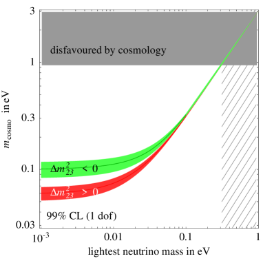
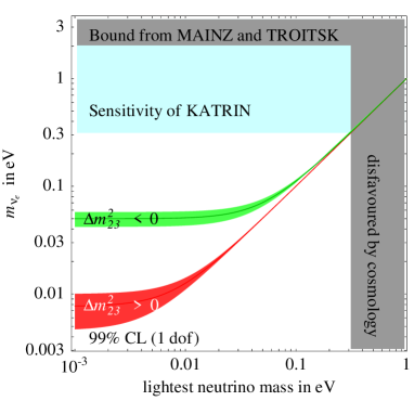
Figure 6: $99\%$ CL expected ranges for the parameters $m_{\rm cosmo}=m_{1}+m_{2}+m_{3}$ probed by cosmology (fig. 6a) and $m_{\nu_{e}}\equiv(m\cdot m^{\dagger})^{1/2}_{ee}$ probed by $\beta$-decay (fig. 6b) as function of the lightest neutrino mass. The darker lines show how the ranges would shrink if the present best-fit values of oscillation parameters were confirmed with negligible error.

3.1 Cosmology

Cosmological observations are mostly sensitive to the sum of neutrino masses: $m_{\rm cosmo}=m_{1}+m_{2}+m_{3}$, that according to standard cosmology controls the energy fraction $\Omega_{\nu}$ in non relativistic neutrinos as $\Omega_{\nu}h^{2}=m_{\rm cosmo}/93.5{\rm eV}$ where as usual $h$ parameterizes the present value of the Hubble constant as $h\equiv H_{\rm today}/(100\hbox{km/s\,Mpc})$. Cosmology does not distinguish Majorana from Dirac neutrino masses.

In order to convert CMB and LSS data into a constraint on neutrino masses one needs to assume a cosmological model. The “WMAP constraint” [31] assumes that the observed structures are generated by Gaussian adiabatic primordial scalar fluctuations with flat spectral index $n$ evolved in presence of the known SM particles, of cold dark matter and of a cosmological constant. This standard model of cosmology seems consistent with all observations. Furthermore, it is assumed that observed luminous matter tracks the dark matter density up to a scale-independent bias factor. The data-set includes Lyman-$\alpha$ data about structures on scales so small that perturbations are no longer a minor correction to a uniform background. These data are sensitive to neutrino masses (and thereby somewhat affect the global cosmological fit) but might be affected by non linear evolution effects, which are not fully understood. In summary, cosmology presently gives the dominant constraint, which however rests on untested assumptions and on risky systematics.

In the future the sensitivity to neutrino oscillations will improve thanks to better CMB data and to new LSS measurements less plagued by potential systematic effects. If cosmology were simple (e.g. a spectral index $n=1$, no tensor fluctuations,…) then it seems possible to detect even neutrino masses as small as allowed by oscillation data [32]. The expected ranges of $m_{\rm cosmo}$ are reported in the lowest row of table 1 in the limiting case where the lightest neutrino is massless, and in fig. 6a in the general case.

3.2 Direct search via $\beta$ decay

$\beta$-decay experiments dominantly probe the quantity $m_{\nu_{e}}\equiv(m\cdot m^{\dagger})_{ee}^{1/2}$. If neutrinos are quasi-degenerate, $m_{\nu_{e}}$ is their common mass. The MAINZ and TROITSK experiments obtained comparable limits: $m_{\nu_{e}}^{2}=-1.2\pm 2.2\pm 2.1$ eV² [33] and $m_{\nu_{e}}^{2}=-2.3\pm 2.5\pm 2.0$ eV² [34] respectively. The 95% bounds quoted by the experimental collaborations agree with the values obtained in Gaussian approximation. Thus, we combine the two measurements by summing errors in quadrature and get

$$m_{\nu_{e}}^{2}=-1.7\pm 2.2\mbox{ eV}^{2}\qquad\hbox{i.e.}\qquad m_{\nu_{e}}<2.0\,{\rm eV}\hbox{ at 99 \% C.L.}$$ (12)

In order to study what oscillation data imply on the value of $m_{\nu_{e}}$ we write it in terms of the neutrino masses $m_{i}$ and of the mixing angles $\theta_{ij}$ as

$$m_{\nu_{e}}=\bigg{[}\cos^{2}\theta_{13}(m_{1}^{2}\cos^{2}\theta_{12}+m_{2}^{2}\sin^{2}\theta_{12})+m_{3}^{2}\sin^{2}\theta_{13}\bigg{]}^{1/2}.$$ (13)

In the case of normal mass hierarchy, $m_{1}\ll m_{2}\ll m_{3}$ oscillation data imply the 99% CL range $m_{\nu_{e}}=(4.6\div 10)\,{\rm meV}$. In the case of inverted hierarchy, $m_{3}\ll m_{1}<m_{2}$ one gets $m_{\nu_{e}}=(42\div 57)\,{\rm meV}$. The last number if a factor 5 below the planned sensitivity of Katrin [35].

It is immediate to obtain the ranges corresponding to the generic case of a non vanishing lightest neutrino mass $m_{\rm lightest}$ (where $m_{\rm lightest}=m_{1}$ in the case of normal hierarchy and $m_{\rm lightest}=m_{3}$ in the case of inverted hierarchy). As clear from the definition $m_{\nu_{e}}^{2}\equiv(m\cdot m^{\dagger})_{ee}$ or from the more explicit expression in eq. (13) one just needs to add $m_{\rm lightest}^{2}$ to $m_{\nu_{e}}^{2}$. The resulting bands at $99\%$ C.L.  are plotted in fig. 6b.

3.3 Neutrino-less double-beta decay

Updating the results of [30], in the 3 neutrino framework we discuss the connection with oscillations, the bound from $0\nu 2\beta$ on neutrino masses and the possible hint of a signal.

IGEX, CUORICINO and nuclear uncertainties.

First, we recall that recently two experiments produced new relevant data. The first is IGEX [36], now terminated, which used 86% enriched ⁷⁶Ge (with exposure $7\cdot 10^{25}$ nuclei$\cdot$yr). The second is Cuoricino [37], now running, which uses 34% natural ¹³⁰Te (with exposure $1.4\cdot 10^{24}$ nuclei$\cdot$yr, and the plan to collect 10 times more data in about 6 years). Both experiments reached a good level of background (about $0.18/\rm keV\cdot kg\cdot yr$), good detection efficiencies of 70% and 84%, and respectable energy resolutions, the full width at half maximum being 4 keV and 7 keV respectively. For comparison, the Heidelberg–Moscow (HM) data-set with pulse-shape-discrimination [38] has exposure $2.5\cdot 10^{26}$ nuclei$\cdot$yr and background $0.06/\rm(keV\cdot kg\cdot yr)$.

As in [30] we quote the limits on $|m_{ee}|$ adopting the $0\nu 2\beta$ nuclear matrix elements ${\cal M}_{0}$ computed in [39]. To use a different calculation with matrix element ${\cal M}$, just rescale by the factor $h={\cal M}_{0}/{\cal M}$, which depends on the nucleus studied. We always explicit the factors $h$ when quoting an experimental result on $0\nu 2\beta$. We prefer to show such uncertainty explicitly rather than attempting to evaluate the theoretical error on matrix elements. Different published computations find $h$ in the following ranges

$$0.3~{}\cite[cite]{[\@@bibref{}{staudt92}{}{}]}<h({}^{76}{\rm Ge})<2.4~{}\cite[cite]{[\@@bibref{}{caurier96}{}{}]},\qquad 0.4~{}\cite[cite]{[\@@bibref{}{staudt92}{}{}]}<h({}^{130}{\rm Te})<2.7~{}\cite[cite]{[\@@bibref{}{rodin03}{}{}]}.$$ (14)

When comparing two results on $|m_{ee}|$ obtained with different nuclei one needs to consider the ratios of $h$, e.g., $h(^{130}\mbox{Te})/h(^{76}\mbox{Ge})$. This quantity is also uncertain, spanning the following range:

$$0.3~{}\cite[cite]{[\@@bibref{}{engel88}{}{}]}<h(^{130}\mbox{Te})/h(^{76}\mbox{Ge})<1.7~{}\cite[cite]{[\@@bibref{}{rodin03}{}{}]}.$$ (15)

Nucleus and		observed	background	expected	99% C.L. bound
experiment		events, $n$	events, $b$	signal	on $|m_{ee}|/h$
76Ge	HM [38]	21	$20.4\pm 1.6$	76 $\,|m_{ee}/{\rm eV}|^{2}/h^{2}$	0.44 eV
76Ge	IGEX [36, 44]	9.6	$17.2\pm 2\phantom{.0}$	23.5$|m_{ee}/{\rm eV}|^{2}/h^{2}$	0.55 eV
130Te	Cuoricino [45, 37]	24	$35.2\pm 4\phantom{.0}$	21.5$|m_{ee}/{\rm eV}|^{2}/h^{2}$	0.62 eV

Table 2: Numbers of observed events, expected background and predicted signal in the most sensitive $0\nu 2\beta$ experiments. The last column shows the $99\%$ C.L. constraint on $|m_{ee}|/h$, where $h\sim 1$ parameterizes the uncertain $0\nu 2\beta$ nuclear matrix element and depends on the nucleus studied.

Now we convert $0\nu 2\beta$ data into a constraint on $|m_{ee}|$ following the same simple procedure employed by the HM collaboration [38]: the Poisson likelihood of having $s$ signal events is ${\cal L}(s)\propto e^{-s}(b+s)^{n}$, where $n$ and $b$ are the numbers of observed and expected background events in the 3$\sigma_{E}$ window around the $Q$ value of the $0\nu 2\beta$, and $\sigma_{E}$ is the energy resolution of the apparatus. We therefore evaluate $n$ and $b$ in the 10 keV region around $Q=2039$ keV for IGEX [36, 44] and in the 18 keV region around $Q=2529$ keV for Cuoricino [45, 37]. Results are collected in table 2. For both experiments the observed number of events is slightly below the expected background. In this paper we systematically employ the Gaussian approximation: the $99\%$ constraint (2.58$\sigma$) on $|m_{ee}|$ is computed by defining $\chi^{2}\equiv-2\ln{\cal L}$, marginalizing it with respect to the uncertainty in the background, and finally quoting the value of $|m_{ee}|$ such that $\chi^{2}(m_{ee})-\chi^{2}(m_{ee}=0)=2.58^{2}$. Different approaches to statistical inference give slightly different constraints.

Since HM and IGEX are both based on ⁷⁶Ge, it is possible to obtain a more stringent combined bound, $|m_{ee}|<0.38\ h$ eV.

         

         

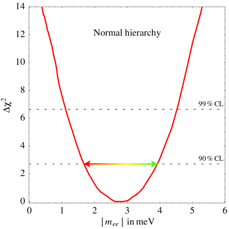
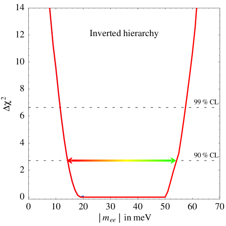
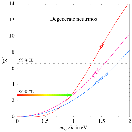
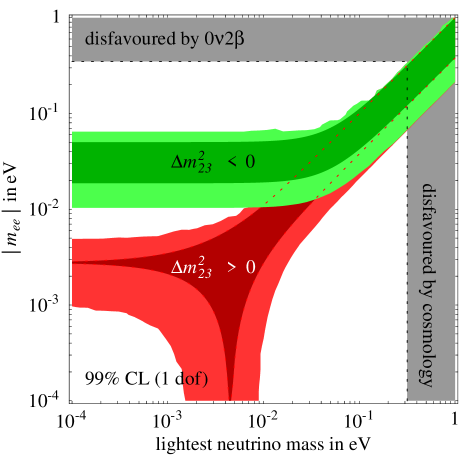
Figure 7: Predictions for $|m_{ee}|$ assuming a hierarchical (fig. 7a) and inverted (fig. 7b) neutrino spectrum. In fig. 7c we update the upper bound on the mass of quasi-degenerate neutrinos implied by $0\nu 2\beta$ searches. The factor $h\approx 1$ parameterizes the uncertainty in the nuclear matrix element (see sect. 2.1). In fig. 7d we plot the $99\%$ CL range for $m_{ee}$ as function of the lightest neutrino mass, thereby covering all spectra. The darker regions show how the $m_{ee}$ range would shrink if the present best-fit values of oscillation parameters were confirmed with negligible error.

Inference on $|\mbox{\normalsize\boldmath$m$}_{ee}|$ from oscillations.

Using the latest oscillation data, we study the expected range of $|m_{ee}|$. We follow the procedure described in [30]. Assuming three CPT-invariant massive Majorana neutrinos we get:

• In the case of normal hierarchy (i.e. $m_{1}\ll m_{2}\ll m_{3}$, or $\Delta m^{2}_{23}>0$) the $ee$ element of the neutrino mass matrix probed by $0\nu 2\beta$ decay experiments can be written as $|m_{ee}|=|e^{2i\alpha}m_{ee}^{\rm sun}+e^{2i\beta}m_{ee}^{\rm atm}|$ where $\alpha,\beta$ are unknown Majorana phases and the ‘solar’ and ‘atmospheric’ contributions can be predicted from oscillation data. The solar contribution to $m_{ee}$ is $m_{ee}^{\rm sun}=(\Delta m^{2}_{12})^{1/2}\sin^{2}\theta_{12}\cos^{2}\theta_{13}=(2.78\pm 0.22)~{}\,\hbox{meV}$. The bound on $\theta_{13}$ implies $m_{ee}^{\rm atm}=(\Delta m^{2}_{23})^{1/2}\sin^{2}\theta_{13}<1.7\,\hbox{meV}$ at 99% CL. By combining these two contributions we get the range reported in table 1. The precise prediction is shown in fig. 7a. Unlike in our previous results [30], a non zero contribution is now guaranteed at high confidence level, because data now tell that the ‘solar’ contribution is larger than the ‘atmospheric’ contribution, so that a cancellation is not possible.

• In the case of inverted hierarchy (i.e. $m_{3}\ll m_{1}\approx m_{2}$, or $\Delta m^{2}_{23}<0$), from the prediction $|m_{ee}|\approx|\Delta m^{2}_{23}|^{1/2}\times|\cos^{2}\theta_{12}+e^{2i\alpha}\sin^{2}\theta_{12}|\cos^{2}\theta_{13}$ we get the range reported in table 1 (see also [46]). The precise prediction is shown in fig. 7b. The main uncertainty on $|m_{ee}|$ is due to the Majorana phase $\alpha$, rather than to the oscillation parameters. If the present central values were confirmed with infinite precision we would still have the loose range $|m_{ee}|=(19\div 50)\,{\rm meV}$ at any C.L.

The $|m_{ee}|$ ranges for normal and inverted hierarchy do not overlap. Values of $|m_{ee}|$ outside these ranges are possible if the lightest neutrino mass is not negligible, as shown in fig. 7d. In the inverted hierarchy case ($\Delta m^{2}_{23}<0$) a non zero lightest neutrino mass can only make $|m_{ee}|$ larger than in case b). The darker regions in fig. 7d show how the predicted range of $|m_{ee}|$ would shrink if the present best-fit values of oscillation parameters were confirmed with infinite precision. The two funnels present for $\Delta m^{2}_{23}>0$ have an infinitesimal width because we assume $\theta_{13}=0$ and would have a finite width if $\theta_{13}\neq 0$.

• The case of quasi-degenerate neutrinos with mass $m_{\nu_{e}}$ corresponds to the upper region of fig. 7d. $|m_{ee}|$ and $m_{\rm cosmo}$ are related to $m_{\nu_{e}}$ as

  $$m_{\rm cosmo}=3m_{\nu_{e}}\qquad\hbox{and}\qquad 0.24\,m_{\nu_{e}}<|m_{ee}|<m_{\nu_{e}}\hbox{ at $99\%$ C.L.}$$ (16)

  The lower bound on $|m_{ee}|$ holds thanks to the fact that solar data exclude a maximal solar mixing and that CHOOZ requires a small $\theta_{13}$.

Upper bound on neutrino masses from $0\nu 2\beta$.

The above result means that by combining oscillation data with the $0\nu 2\beta$ upper bound on $|m_{ee}|$ implies an upper bound on the parameter $m_{\nu_{e}}$ probed by $\beta$ decay experiments [30]. In view of present values, such $m_{\nu_{e}}$ corresponds to the common mass of quasi-degenerate neutrinos. This bound is shown in fig. 7c, and depends on the $0\nu 2\beta$ nuclear matrix elements, parameterized by the uncertain factors $h\sim 1$. Therefore the results of Cuoricino, obtained with a nucleus different than HM and IGEX, add confidence in the result. For $h=1$ the combined constraint is $m_{\nu_{e}}/h<1.0\,{\rm eV}$ at $99\%$ C.L. This constraint is stronger than the $\beta$-decay constraint (but holds under the additional assumption that neutrinos are Majorana particles) and is weaker than the cosmological constraint (but needs no assumptions about cosmology).

In all above discussions we employed the bound on $|m_{ee}|$ from HM data, as published by the HM collaboration [38].

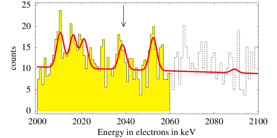
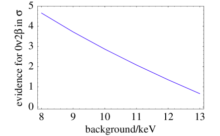
Figure 8: Fig. 8a: the latest HM data [13] ($71.7{\rm kg}\cdot{\rm yr}$) used to claim a $4.2\sigma$ evidence for $0\nu 2\beta$. Fig. 8b: the statistical significance of the $0\nu 2\beta$ signal, as function of the assumed flat component of the background.

Remarks on the hint for $0\nu 2\beta$.

While the HM collaboration used their data to set a bound on $|m_{ee}|$, some members of the HM collaboration reinterpreted the data as an evidence for $0\nu 2\beta$ [12]. According to this claim, the latest HM data [13] plotted in fig. 8a contain a $4.2\sigma$ evidence for a $0\nu 2\beta$ peak (indicated by the arrow). In these latest results the peak is more visible than in latest published HM data [38], partly thanks to higher statistics (increased from 53.9 to 71.7 kg yr) and partly thanks to an ‘improved analysis’ [13]).

This claim is controversial, mainly because one needs to fully understand the background before being confident that a signal has been seen. In order to allow a better focus on this key issue, we present fig. 8b, which should be uncontroversial. It shows the statistical significance of the $0\nu 2\beta$ signal as a function of the true background level $b$, assumed to be quasi-flat close to the $Q$-value of $0\nu 2\beta$, $Q\approx 2039\,{\rm keV}$. The crucial issue is: how large is $b$? The HM collaboration earlier claimed [38] $b=(13.6\pm 0.7){\rm events}/(71.7\,{\rm kg}\,{\rm yr}\cdot{\rm keV})$. In such a case the statistical significance of the signal would be less than $1\sigma$, see fig. 8b. This can be considered as the upper bound on $b$ computed assuming that all events in a wider range around $Q$ come from a quasi-flat background.

A statistically significant hint for $0\nu 2\beta$ is obtained if one can show that $b$ is lower. The continuous line in fig. 8a shows a fit of HM data using a tentative model of the background [12], assumed to have a quasi-flat component $b$ (mainly due to ‘natural’ and ‘cosmogenic’ radioactivity) plus some peaks due to faint $\gamma$ lines of ²¹⁴Bi, which is a radioactive impurity present in the apparatus (from the ²³⁸U decay chain). Their positions and intensities can be estimated from tables of nuclear decays; however they are modified by ${\cal O}(1)$ factors by detector-related effects which depend on the unknown localization of ²¹⁴Bi (see [13] and ref.s therein). The fit in fig. 8a is performed by allowing the intensity of each line to freely vary. In this way part of the background is interpreted as ²¹⁴Bi peaks, thereby reducing the quasi-flat component $b$. Proceeding in this way, we find that the statistical significance of the $0\nu 2\beta$ signal is about $2.7\sigma$. This is the best we can do with the data at our disposal. This kind of analysis was proposed in [30] and has been adopted in [13].

However, some details in its implementation prevent this analysis from fully reaching its goal, which is determining $b$ from regions with no peaks. 1) The latest data have been published only below 2060 keV. (Above 2060 keV in fig. 8a we plotted HM data artificially rescaled to account for the larger statistics). Below 2060 keV there are little energy ranges with no peaks. Including the old data above 2060 keV in the fit would reduce the significance of the signal down to about $2.2\sigma$. 2) HM data contain hints of extra unidentified spurious peaks at specific energies (at 2030 keV and above 2060 keV). Fitting data assuming that these extra peaks can be present at arbitrary energies with arbitrary intensities reduces $b$ and enhances the statistical significance of the signal.

Various future experiments plan to test the claim of [12]. The most direct test requires using the same technique (germanium detectors) but in the worst case, when the observed hint of a signal is due to some irreducible (hypothetical) background, a safe test requires a different type of detector. As previously discussed Cuoricino employs a different nucleus: its capabilities relative to HM and IGEX depend on the uncertain relative nuclear matrix element. For instance, with the lowest value in eq. (15) Cuoricino is already testing the claim of [12]; for intermediate values new data of Cuoricino will significantly test the claim; for the highest value Cuoricino will be not sufficient.

In our view, a discussion of what should be considered as a convincing evidence for $0\nu 2\beta$, is anyway useful or necessary, because any experiment (past and future) needs to confront with this issue.

4 Conclusions

Assuming oscillations of three active massive neutrinos we updated the determination of the oscillations parameters, at the light of latest experimental data. Results are shown in table 1 and in fig. 1. We notice that the parameters $\Delta m^{2}_{12},\theta_{12},\theta_{23}$ are now dominantly determined by simple and robust sub-sets of data, such that simple arguments give the same final result as global analyses. Pieces of data that play a sub-dominant rôle in parameter determination allow to test our assumptions: e.g. allowing neutrinos and anti-neutrinos to have different masses and mixings gives the CPT-violating fit of fig. 3. Present data do not contain evidence for extra effects.

We also tried to study in a simple and general way related topics, such as the determination of the limiting survival probability of solar neutrinos at small and large energies, the present knowledge of solar neutrino fluxes, etc. Approximated general results have been compared with ‘exact’ results of global fits performed in specific cases.

Finally, updating the results of [30], we studied how oscillation data allow to infer the combination of neutrino masses probed by cosmology, $\beta$-decay and $0\nu 2\beta$-decay experiments, and discussed the present experimental situation.

References

- [1] The results of the Homestake experiment are reported in B.T. Cleveland et al., Astrophys. J. 496 (1998) 505.
- [2] Latest Gallex and SAGE data have been presented in a talk by C. Cattadori at the ‘Neutrino 2004’ conference (Paris, 14-19 June), web site neutrino2004.in2p3.fr.
- [3] Gallex collaboration, Phys. Lett. B447 (1999) 127.
- [4] SAGE Collaboration, J. Exp. Theor. Phys. 95 (2002) 181 [astro-ph/0204245].
- [5] Super-Kamiokande collaboration, hep-ex/0205075.
- [6] SNO collaboration, nucl-ex/0204008 and nucl-ex/0204009.
- [7] SNO collaboration, nucl-ex/0502021.
- [8] KamLAND collaboration, hep-ex/0406035.
- [9] SuperKamiokande collaboration, hep-ex/0501064.
- [10] MACRO collaboration, Phys. Lett. B566 (2003) 35 [hep-ex/0304037].
- [11] K2K collaboration, hep-ex/0411038.
- [12] H. V. Klapdor-Kleingrothaus, A. Dietz, H. L. Harney and I. V. Krivosheina, Mod. Phys. Lett. A 16 (2001) 2409 [hep-ph/0201231].
- [13] H. V. Klapdor-Kleingrothaus, A. Dietz, I. V. Krivosheina and O. Chkvorets, Nucl. Instrum. Meth. A 522 (2004) 371 [hep-ph/0403018].
- [14] LSND collaboration, Phys. Rev. D64 (2001) 112007 [hep-ex/0104049].
- [15] A. Strumia and F. Vissani, JHEP 0111 (2001) 048 [hep-ph/0109172].
- [16] J.N. Bahcall, S. Basu, M.H. Pinsonneault, Astrophys. J. 555 (2001) 990 [astro-ph/0010346].
- [17] LUNA collaboration, nucl-ex/0312015.
- [18] P. Creminelli et al., J. HEP 05 (052) 2001 [hep-ph/0102234]. Its e-print version, has been updated including the recent data from SNO.
- [19] A. Strumia, hep-ph/0201134. The solar CPT-violating fit has been re-emphasized in H. Murayama, Phys. Lett. B 597 (2004) 73 [hep-ph/0307127] and in A. de Gouvea, C. Peña-Garay, hep-ph/0406301. The atmospheric CPT-violating fit has been also studied by the SK collaboration, see the talk by E. Kearns at the Neutrino 2004 conference (Paris, 14-19 June), web site neutrino2004.in2p3.fr. See also M. C. Gonzalez-Garcia, M. Maltoni and T. Schwetz, Phys. Rev. D 68 (2003) 053007.
- [20] A. Strumia and R. Barbieri, JHEP 12 (2000) 016. Its e-print version, hep-ph/0011307, contains updates and additional discussions not present in the published version.
- [21] S. Goswami, A. Bandyopadhyay and S. Choubey, Nucl. Phys. Proc. Suppl. 143 (2005) 121 [hep-ph/0409224]. B. S. Koranga, M. Narayan and S. Uma Sankar, hep-ph/0503092.
- [22] J.N. Bahcall, C. Peña-Garay, JHEP 004 (2003) 0311. A. Bandyopadhyay, S. Choubey, S. Goswami, S.T. Petcov, hep-ph/0410283.
- [23] For a recent extensive study see M. Cirelli et al, Nucl. Phys. B708 (2005) 215 [hep-ph/0403158]. For short summaries see A. Strumia, Nucl. Phys. Proc. Suppl. 143 (2005) 144 [hep-ph/0407132] and M. Cirelli, astro-ph/0410122.
- [24] C. Galbiati, A. Pocar, D. Franco, A. Ianni, L. Cadonati, S. Schonert, hep-ph/0411002.
- [25] J. N. Bahcall, M. C. Gonzalez-Garcia and C. Pena-Garay, Phys. Rev. Lett. 90 (2003) 131301.
- [26] For a recent summary of capabilities of neutrino beam experiments see M. Lindner, hep-ph/0503101. If it seems practically impossible to discriminate the kind of neutrino mass hierarchy with oscillation experiments, as recently discussed in A. de Gouvea, J. Jenkins and B. Kayser, hep-ph/0503079.
- [27] Y. Itow et al., “The JHF-Kamioka neutrino project”, hep-ex/0106019
- [28] P. Huber, M. Lindner, T. Schwetz and W. Winter, Nucl. Phys. B 665 (2003) 487 [hep-ph/0303232].
- [29] O.L.G. Peres, A.Yu. Smirnov, Nucl. Phys. B680 (2004) 479 [hep-ph/0309312].
- [30] F. Feruglio, A. Strumia and F. Vissani, Nucl. Phys. B 637 (2002) 345 [addendum-ibid. B 659 (2003) 359] [hep-ph/0201291].
- [31] C.L. Bennett et al., astro-ph/0302207 and D.N. Spergel et al., astro-ph/0302209. The WMAP constraint is similar to previous analyses, e.g. A. Lewis, S. Bridle, Phys. Rev. D66 (2002) 103511. Other (sometimes more conservative) analysis find similar (sometimes weaker) bounds: S. Hannestad, JCAP 0305 (2003) 004 [astro-ph/0303076], S.W. Allen, R.W. Schmidt, S.L. Bridle, Mon. Not. Roy. Astron. Soc. 346 (2003) 593 [astro-ph/0306386], M. Tegmark et al. [SDSS Collaboration], Phys. Rev. D69 (2004) 103501 [astro-ph/0310723] V.Barger et al., Phys. Lett. B595 (2004) 55 [hep-ph/0312065], P. Crotty, J. Lesgourgues, S. Pastor, Phys. Rev. D69 (2004) 123007 [hep-ph/0402049], U. Seljak et al., astro-ph/0407372.
- [32] For recent discussions see S. Hannestad, Phys. Rev. D 67 (2003) 085017 [astro-ph/0211106]; J. Lesgourgues, S. Pastor and L. Perotto, Phys. Rev. D 70 (2004) 045016 [hep-ph/0403296].
- [33] MAINZ collaboration, hep-ex/0412056.
- [34] TROITSK collaboration, Phys. Lett. B 460 (1999) 227. The latest results have been presented in a talk by V. Lobashev at the XI International Workshop on “Neutrino Telescopes” (Venezia, Feb. 22-25 2005).
- [35] KATRIN web site: www-ik1.fzk.de/tritium.
- [36] IGEX collaboration, Phys. Rev. C 59 (1999) 2108.
- [37] Cuoricino collaboration, hep-ex/0501034.
- [38] Heidelberg-Moscow collaboration, Eur. Phys. J. A 12 (2001) 147 [hep-ph/0103062].
- [39] A. Staudt et al., Europh. Lett 13 (1990) 31.
- [40] A. Staudt et al., Phys. Rev. C46 (1992) 871.
- [41] E. Caurier, Phys. Rev. Lett. 77 (1996) 1954.
- [42] V.A. Rodin et al., Phys. Rev. C68 (2003) 044302.
- [43] J. Engel et al., Phys. Rev. C37 (1988) 871.
- [44] C. E. Aalseth et al., Mod. Phys. Lett. A 17 (2002) 1475 [hep-ex/0202018].
- [45] Cuoricino collaboration, Phys. Lett. B 584 (2004) 260.
- [46] H. Murayama and C. Pena-Garay, Phys. Rev. D 69 (2004) 031301 emphasized that the lower bound on in the case of inverted hierarchy is ‘robust’ and found a value in agreement with results in [30].