Nonperturbative renormalization for
2PI effective action techniques

Nonperturbative approximation schemes based on two-particle irreducible (2PI) effective actions provide an important means for our current understanding of (non-)equilibrium quantum field theory. A remarkable property is their renormalizability, since these approximations involve selective summations to infinite perturbative orders. In this paper we show how to renormalize all $n$-point functions of the theory, which are given by derivatives of the 2PI-resummed effective action $\Gamma[\phi]$ for scalar fields $\phi$. This provides a complete description in terms of the generating functional for renormalized proper vertices, which extends previous prescriptions in the literature on the renormalization for 2PI effective actions. The importance of the 2PI-resummed generating functional for proper vertices stems from the fact that the latter respect all symmetry properties of the theory and, in particular, Goldstone’s theorem in the phase with spontaneous symmetry breaking. This is important in view of the application of these techniques to gauge theories, where Ward identities play a crucial role.

1 Introduction

Selective summations to infinite order in perturbation theory often play an important role in vacuum, thermal equilibrium or nonequilibrium quantum field theory. A prominent example concerns theories with bosonic field content such as QCD, QED or scalar theories at high temperature, where standard perturbative expansions are plagued by infrared singularities. Screening effects can be taken into account e.g. by resumming so-called hard thermal loops [1]. The resulting resummed perturbation theory, however, can reveal a poor convergence behavior and typically requires further summations [2]. It has been pointed out that improved behavior may be based on expansions of the two-particle irreducible (2PI) effective action [3]. This has recently been demonstrated for scalar theories, where a dramatically improved convergence behavior is observed once systematic loop- or coupling-expansions of the 2PI effective action are employed without further assumptions [4]. These 2PI approximation schemes also play a crucial role for our understanding of quantum fields out-of-equilibrium [5, 6]. There, infinite summations are needed to obtain approximations which are uniform in time. 2PI techniques provide for the first time the link between far-from-equilibrium dynamics at early times and late-time thermalization in quantum field theory [7, 8, 9, 10, 11]. The good convergence properties of the approach have also been observed in the context of classical statistical field theories, where comparisons with exact results are possible [12], or in applications to universal properties of critical phenomena [13].

The 2PI expansions are known to be consistent with global symmetries [14, 15, 16]. However, Ward identities may not be manifest at intermediate calculational steps of a 2PI resummation scheme. To obtain the correct symmetry properties for physical results requires a consistent renormalization procedure for the 2PI-resummed effective action $\Gamma[\phi]$. The latter is the generating functional for the proper vertices by derivatives with respect to the field $\phi$. Very important progress in this direction has been made in Refs. [16, 17]. It has been shown, in particular, that the resummation equation for the two-point function in the context of scalar $\varphi^{4}$-theories can be made finite by adjusting a finite number of local counterterms. A similar analysis [20] has recently been performed for the 2PI $1/N$-expansion [8, 21]. Although this allows one to compute various physical quantities such as the thermodynamic pressure, we emphasize that the renormalization presented in these works is not sufficient to fix all counterterms needed to compute the proper vertices encoded in $\Gamma[\phi]$. The aim of this work is to provide this missing prescription for general approximations schemes, including systematic loop-, coupling- or $1/N$-expansions. We exemplify these techniques using scalar field theories for simplicity. Very similar techniques as those employed here can be used for more complicated systems, including fermionic or gauge degrees of freedom, or for higher $n$PI effective actions. The importance of the 2PI-resummed generating functional $\Gamma[\phi]$ for proper vertices stems from the fact that the latter respect all symmetry properties of the theory and, in particular, Goldstone’s theorem in the phase with spontaneous symmetry breaking. This is a crucial step towards the renormalization for 2PI-resummed effective actions in gauge theories, where Ward identities play a particularly important role. The application of our techniques to the latter will be presented in a separate work [22].

It is a remarkable property that 2PI approximations schemes are renormalizable, since they involve selective summations to infinite perturbative orders. The proof requires to show that all $n$-point functions of the theory, which are given by derivatives of the effective action, can be renormalized. This is exemplified in the present work for scalar field theories with quartic self-interactions. The non-trivial character of this result is two-fold: firstly, the divergences due to the infinite selective summation can be absorbed in a finite number of counterterms and, secondly, the procedure involves only standard “local” counterterms despite the non-local character of the 2PI summation. Furthermore, the renormalization procedure is medium-independent. Thus no temperature, chemical potential or even time-dependence is hidden in the counterterms. We have published previously a first application of our methods to resolve the convergence problems of perturbative expansions at high temperature in Ref. [4]. The aim was to demonstrate the applicability for practical calculations, before presenting in detail the discussion of the somewhat contrived foundations. We mention that a summary of the present work was presented in [23].

The paper is organized as follows: Sec. 2 describes basics of the 2PI approach required for the present discussion. In Sec. 2.2, we explicitly construct the $n$-point functions of the theory in terms of functional derivatives of the 2PI effective action. These derivatives involve summations of infinite series of diagrams, which can be all conveniently generated by a single four-point vertex-function through an integral, Bethe-Salpeter–type equation. Once expressed in terms of the solution of this equation, the renormalization analysis for $n$-point functions is considerably simplified. Sec. 3 presents a comprehensive discussion of the nonperturbative renormalization to be performed here and will be of interest for readers who are not interested in going through the technical details of the proof, which we present in Sec. 4. We discuss in Sec. 5 that once the theory has been renormalized in the symmetric phase, no new divergences appear for a non-vanishing field expectation value. Various aspects concerning symmetries and renormalization for the case of multiple scalar field components and the application to the 2PI $1/N$-expansion are discussed in Sec. 6. We end with a summary and conclusions in Sec. 7. Appendix LABEL:sec:appcorrel is devoted to the derivation of useful identities between the various functional derivatives of the 2PI effective action, and Appendix LABEL:2PItop discusses some of their topological properties for diagrammatics.

2 The 2PI-resummed effective action

2.1 Definition

All information about the quantum theory can be obtained from the (1PI) effective action $\Gamma[\phi]$, which is the generating functional for proper vertex functions. This effective action is represented as a functional of the field expectation value or one-point function $\phi$ only. In contrast, the 2PI effective action $\Gamma_{\rm 2PI}[\phi,G]$ is written as a functional of $\phi$ and the connected two-point function $G$ by introducing an additional bilinear source in the defining functional integral [14, 18]. Higher functional representations, so-called $n$PI effective actions $\Gamma_{\rm nPI}[\phi,G,V_{3},\ldots,V_{n}]$, are constructed accordingly and include in addition the three-point, four-point, …, and $n$-point functions or the corresponding proper vertices $V_{3},\ldots,V_{n}$ [14, 24, 25]. The different functional representations of the effective action are equivalent in the sense that they agree for the exact theory in the absence of additional sources:

$$\Gamma[\phi]=\Gamma_{\rm 2PI}[\phi,G=\bar{G}(\phi)]=\cdots=\Gamma_{\rm nPI}[\phi,G=\bar{G}(\phi),\ldots,V_{n}=\bar{V}_{n}(\phi)]\,.$$ (2.1)

The absence of additional sources corresponds to the stationarity conditions [14, 24]

$$\frac{\delta\Gamma_{\rm nPI}}{\delta G}\Big{|}_{G=\bar{G}}=0\quad,\ldots,\quad\frac{\delta\Gamma_{\rm nPI}}{\delta V_{n}}\Big{|}_{V_{n}=\bar{V}_{n}}=0\,,$$ (2.2)

by which the $n$-point functions are determined self-consistently and become implicit functions of the field: $G=\bar{G}(\phi)$, $V_{3}=\bar{V}_{3}(\phi)$, …, $V_{n}=\bar{V}_{n}(\phi)$.

The importance of different functional representations for the effective action stems from the fact that one typically cannot solve the theory exactly. Higher $n$PI effective actions turn out to provide a very efficient tool to build systematic nonperturbative approximation schemes. For instance, a loop expansion of the 1PI effective action to a given order differs in general from an expansion of $\Gamma_{\rm 2PI}[\phi,G]$ to the same number of loops. The 2PI loop-expansion truncated at a given order can be seen to resum an infinite series of contributions for the 1PI loop-expansion. More generally, any systematic e.g. loop-, coupling-, or $1/N$-expansion of higher effective actions at a given order resums infinitely many contributions in the corresponding expansion of lower effective actions. Higher effective actions, therefore, provide a powerful tool to devise systematic nonperturbative approximation schemes for the calculation of $\Gamma[\phi]$. In the following we concentrate on the 2PI effective action since this has been the most frequently used so far.

In the following we use the abbreviated notation $\phi_{1}\equiv\phi(x_{1})$ and $G_{12}\equiv G(x_{1},x_{2})$, where indices denote the space-time arguments. For theories with more than one field these labels can denote the various field-components as well. We consider a real scalar field theory with classical action for the fluctuating field $\varphi$

$$S[\varphi]=S_{0}[\varphi]+S_{\mbox{\scriptsize int}}[\varphi]\,,$$ (2.3)

with the free (quadratic) part

$$S_{0}[\varphi]=\frac{1}{2}\varphi_{a}\,iG_{0,ab}^{-1}\,\varphi_{b}\,,$$ (2.4)

and where $S_{\mbox{\scriptsize int}}[\varphi]$ represents the interaction part. Here $G_{0}$ is the free field theory propagator and the expectation value of $\varphi$ is denoted by $\phi$. Summation/integration over repeated indices is implied. The corresponding 2PI generating functional can be written as

$$\Gamma_{\mbox{\scriptsize 2PI}}[\phi,G]=S_{0}[\phi]+\frac{i}{2}\,\hbox{Tr }\!\ln G^{-1}+\frac{i}{2}\,\hbox{Tr }G_{0}^{-1}G+\Gamma_{\mbox{\scriptsize int}}[\phi,G]\,,$$ (2.5)

where $\Gamma_{\mbox{\scriptsize int}}$ is given by all closed two-particle-irreducible graphs times an overall factor $(-i)$, with lines representing the (auxiliary) two-point function $G$ [14, 18]. The vertices are obtained in the same way as for the 1PI effective action from the shifted action $S_{\mbox{\scriptsize int}}[\phi+\varphi]$ by collecting all terms higher than quadratic in the fluctuating field $\varphi$ [18]. This provides a functional representation of the theory in terms of the one-point and two-point fields, $\phi$ and $G$. The effective action $\Gamma[\phi]$ is obtained from (2.5) by taking $G$ to be at its physical value, given by the stationarity condition

$$\frac{\delta\Gamma_{\mbox{\scriptsize 2PI}}}{\delta G_{12}}\Big{|}_{{\bar{G}}}=0\,.$$ (2.6)

Using Eq. (2.5), this condition can be rewritten as

$${\bar{G}}_{12}^{-1}(\phi)=G_{0,12}^{-1}-\bar{\Sigma}_{12}(\phi)\,,$$ (2.7)

with the self-energy

$$\bar{\Sigma}_{12}(\phi)\equiv 2i\frac{\delta\Gamma_{\mbox{\scriptsize int}}}{\delta G_{21}}\Big{|}_{{\bar{G}}}\,.$$ (2.8)

The equation for the two-point function (2.7) can be rewritten as an infinite series in terms of the free field theory propagator $G_{0}$:

$${\bar{G}}_{12}(\phi)=G_{0,12}+G_{0,1a}\,\bar{\Sigma}_{ab}(\phi)\,G_{0,b2}+G_{0,1a}\,\bar{\Sigma}_{ab}(\phi)\,G_{0,bc}\,\bar{\Sigma}_{cd}(\phi)\,G_{0,d2}+\ldots$$ (2.9)

Each 2PI diagram with propagator lines associated to $G$ that contributes to $\Gamma_{\rm 2PI}[\phi,G]$, therefore, encodes a selective summation of an infinite series of perturbative diagrams. The effective action $\Gamma[\phi]$ is obtained from a given approximation of the 2PI effective action according to

$$\Gamma[\phi]=\Gamma_{\mbox{\scriptsize 2PI}}[\phi,{\bar{G}}(\phi)]\,.$$ (2.10)

This defines the 2PI-resummed effective action. Equation (2.10) yields an efficient starting point for systematic nonperturbative approximations of the (1PI) effective action. The resummation enters through the solution of the stationarity equation (2.6), which leads to the self-consistent equation (2.7) for ${\bar{G}}(\phi)$. We will use the symbols $\Gamma[\phi]$ and $\Gamma_{\mbox{\scriptsize 2PI}}[\phi,{\bar{G}}(\phi)]$ synonymously in the following.

In order to be able to renormalize all $n$-point functions it is important that all approximations are done on the level of the effective action. Once an approximate $\Gamma_{\mbox{\scriptsize 2PI}}[\phi,G]$ is specified, there are no further approximations involved on the level of the equation of motion (2.7) for ${\bar{G}}(\phi)$. We emphasize that this last property is crucial for the program of renormalization in these self-consistent resummation schemes.

2.2 2PI-resummed $n$-point functions

The functional derivatives of the 2PI-resummed effective action (2.10),

$$\Gamma^{(n)}_{12\ldots n}\equiv\frac{\delta^{n}\Gamma[\phi]}{\delta\phi_{1}\cdots\delta\phi_{n}}\Big{|}_{\bar{\phi}}\,,$$ (2.11)

provide a complete description of the theory in terms of $n$-point functions $\Gamma^{(n)}_{12\ldots n}$ for a given approximation. Here $\phi=\bar{\phi}$ is determined by the stationarity condition

$$\Gamma^{(1)}_{1}\equiv\frac{\delta\Gamma[\phi]}{\delta\phi_{1}}\Big{|}_{\bar{\phi}}=0\,.$$ (2.12)

We emphasize that the functions $\Gamma^{(n)}_{12\ldots n}$ reflect all symmetry properties of the theory. In particular, aspects such as Goldstone’s theorem in the phase with spontaneous symmetry breaking are fulfilled to any order in a systematic 2PI expansion such as loop-, coupling- or $1/N$-expansions [21, 16].

The functions (2.11) are related to derivatives of the 2PI effective action, $\Gamma_{\rm 2PI}[\phi,G]$, through Eq. (2.10). One has, for instance,

$$\frac{\delta\Gamma}{\delta\phi_{1}}=\frac{\delta\Gamma_{\mbox{\scriptsize 2PI}}}{\delta\phi_{1}}\Big{|}_{{\bar{G}}}+\frac{\delta\Gamma_{\mbox{\scriptsize 2PI}}}{\delta G_{ab}}\Big{|}_{{\bar{G}}}\frac{\delta{\bar{G}}_{ab}}{\delta\phi_{1}}=\frac{\delta\Gamma_{\mbox{\scriptsize 2PI}}}{\delta\phi_{1}}\Big{|}_{{\bar{G}}}\,.$$ (2.13)

The last equality arises from Eq. (2.6). Using the representation (2.5) one finds:

$$\frac{\delta\Gamma}{\delta\phi_{1}}=iG_{0,1a}^{-1}\,\phi_{a}+\frac{\delta\Gamma_{\mbox{\scriptsize int}}}{\delta\phi_{1}}\Big{|}_{{\bar{G}}}\,.$$ (2.14)

The functional derivatives of $\Gamma_{\mbox{\scriptsize int}}$, which we call 2PI kernels, play a central role in what follows. In particular, an important feature concerns their two-particle-irreducibility properties. This is discussed in Appendix LABEL:2PItop. It is useful to express the function $\delta{\bar{G}}/\delta\phi$ in terms of 2PI kernels. One has

$$\frac{\delta{\bar{G}}_{12}}{\delta\phi_{3}}=-{\bar{G}}_{1a}{\bar{G}}_{b2}\frac{\delta{\bar{G}}^{-1}_{ab}}{\delta\phi_{3}}={\bar{G}}_{1a}{\bar{G}}_{b2}\frac{\delta\bar{\Sigma}_{ab}}{\delta\phi_{3}}\,,$$ (2.15)

where we have used Eq. (2.7) for the second equality. With this, one obtains for the second derivative of the 2PI resummed effective action:

$$\frac{\delta^{2}\Gamma}{\delta\phi_{1}\delta\phi_{2}} = iG_{0,12}^{-1}+\frac{\delta^{2}\Gamma_{\mbox{\scriptsize int}}}{\delta\phi_{1}\delta\phi_{2}}\Big{|}_{{\bar{G}}}+\frac{\delta^{2}\Gamma_{\mbox{\scriptsize int}}}{\delta\phi_{1}\delta G_{ab}}\Big{|}_{{\bar{G}}}{\bar{G}}_{ac}{\bar{G}}_{db}\frac{\delta\bar{\Sigma}_{cd}}{\delta\phi_{2}}\,.$$ (2.16)

Taking the field derivative of Eq. (2.8) and using Eq. (2.15), one obtains the following integral equation for $\delta\bar{\Sigma}/\delta\phi$:

$$\frac{\delta\bar{\Sigma}_{12}}{\delta\phi_{3}} = \frac{2i\delta^{2}\Gamma_{\mbox{\scriptsize int}}}{\delta G_{12}\delta\phi_{3}}\Big{|}_{{\bar{G}}}+\frac{2i\delta^{2}\Gamma_{\mbox{\scriptsize int}}}{\delta G_{12}\delta G_{ab}}\Big{|}_{{\bar{G}}}{\bar{G}}_{ac}{\bar{G}}_{db}\frac{\delta\bar{\Sigma}_{cd}}{\delta\phi_{3}}\,.$$ (2.17)

The above equation resums the infinite series of “ladder” graphs made of “rungs” $2i\delta^{2}\Gamma_{\mbox{\scriptsize int}}/\delta G^{2}|_{\bar{G}}$ connected by lines ${\bar{G}}$ and “ended” by the kernel $2i\,\delta^{2}\Gamma_{\mbox{\scriptsize int}}/\delta G\delta\phi|_{\bar{G}}$. In the following, we will explain the diagrammatic representation of this equation.

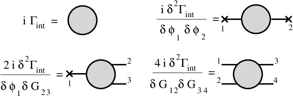
Figure 1: Diagrammatic representation of $\Gamma_{\mbox{\scriptsize int}}$ and its derivatives. Note that external legs do not represent propagators. An overall $i$ and a factor $2$ per each derivative with respect to $G$ are factored out such that the diagrams contributing to the kernels correspond to the standard Feynman rules.

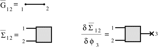
Figure 2: Diagrammatic representations of the functions ${\bar{G}}_{12}$, $\bar{\Sigma}_{12}$ and $\delta\bar{\Sigma}_{12}/\delta\phi_{3}$.

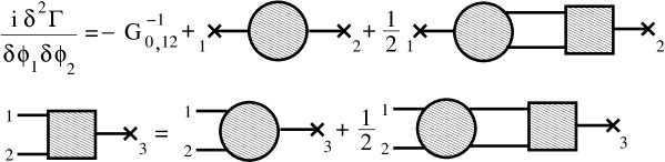
Figure 3: Diagrammatic representation of equations (2.16) and (2.17).

All higher order derivatives can be obtained by differentiating the two equations (2.16) and (2.17). For this purpose, it is useful to introduce the following diagrammatic notation: We represent the 2PI kernels $\sim\delta^{m+n}\Gamma_{\mbox{\scriptsize int}}/\delta\phi^{m}\delta G^{n}\big{|}_{{\bar{G}}}$ having $m+2n$ external legs by dashed circles. Legs ended by crosses represent derivatives with respect to the field $\phi$ and pairs of legs (without crosses) represent derivatives with respect to $G$. For each derivative with respect to $G$ we add a symmetry factor of two. This is illustrated in Fig. 1. Kernels can connect to other structures with lines representing the two-point function ${\bar{G}}$ (cf. Fig. 2). It is useful to introduce a notation for the self-energy $\bar{\Sigma}_{12}$, defined in Eq. (2.8): We use a square box with a pair of legs, which follows the above notation since $\bar{\Sigma}_{12}$ is obtained as a derivative with respect to $G_{12}$. A leg with a cross is added to this box for each derivative with respect to the field $\phi$, as illustrated in Fig. 2. The diagrammatic representation of Eqs. (2.16) and (2.17) is shown in Fig. 3.

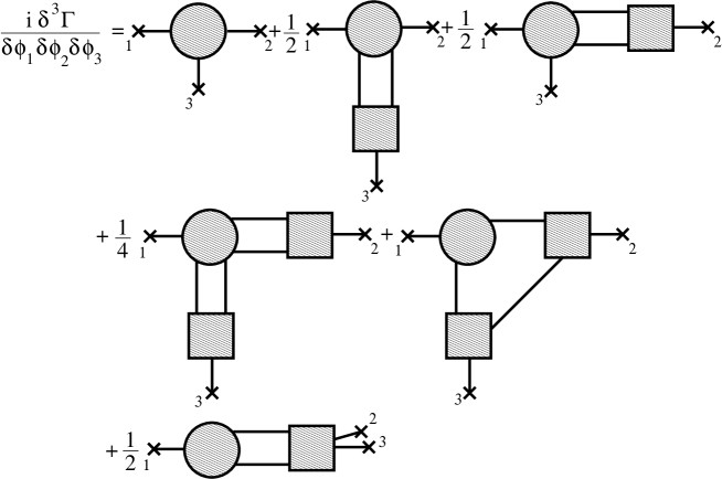
Figure 4: Diagrammatic representation of the third derivative $\delta^{3}\Gamma/\delta\phi_{1}\delta\phi_{2}\delta\phi_{3}$ of the 2PI-resummed effective action. The last graph contains the function $\delta^{2}\bar{\Sigma}/\delta\phi^{2}$, which sums an infinite series of terms described by the integral equation shown in Fig. 5.

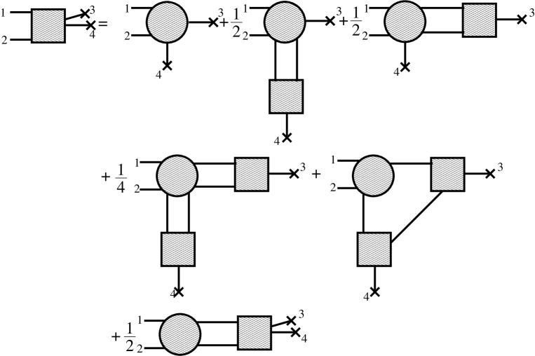
Figure 5: Diagrammatic representation of the integral equation for $\delta^{2}\bar{\Sigma}_{12}/\delta\phi_{3}\delta\phi_{4}$.

Using this diagrammatic notation we show the three-point function $\delta^{3}\Gamma/\delta\phi_{1}\delta\phi_{2}\delta\phi_{3}$ in Fig. 4. One observes the appearance of the function $\delta^{2}\bar{\Sigma}/\delta\phi^{2}$ in the last graph of that figure. By differentiating Eq. (2.17) once, one sees that the latter satisfies an integral equation represented in Fig. 5. Note that these expressions have a very similar structure as those appearing already for the two-point function: According to Eq. (2.16), the expression $\Gamma^{\rm(2)}$ involves a finite number of terms and a term containing the derivative $\delta\bar{\Sigma}/\delta\phi$. The latter is the solution of the linear integral equation (2.17), represented in Fig. 3. By taking further derivatives of Eqs. (2.16) and (2.17) one observes that a similar structure appears for all higher $n$-point functions: $\Gamma^{(n)}$ involves derivatives $\delta^{p}\bar{\Sigma}/\delta\phi^{p}$ with $1\leq p\leq n-1$ and the latter satisfy linear integral equations of the form:

$$\frac{\delta^{p}\bar{\Sigma}_{ab}}{\delta\phi_{1}\cdots\delta\phi_{p}}=\mathcal{A}^{ab}_{1\ldots p}+\frac{2i\delta^{2}\Gamma_{\mbox{\scriptsize int}}}{\delta G_{ab}\delta G_{cd}}\Big{|}_{{\bar{G}}}{\bar{G}}_{ce}{\bar{G}}_{fd}\frac{\delta^{p}\bar{\Sigma}_{ef}}{\delta\phi_{1}\cdots\delta\phi_{p}}\,.$$ (2.18)

Here the function $\mathcal{A}$ involves a finite number of 2PI kernels including lower derivatives $\delta^{k}\bar{\Sigma}/\delta\phi^{k}$ with $1\leq k\leq p-1$. Similarly to Eq. (2.17), the above equation resums an infinite series of ladder graphs with rungs given by $2i\,\delta^{2}\Gamma_{\mbox{\scriptsize int}}/\delta G^{2}|_{\bar{G}}$ and where each ladder is ended by the function $\mathcal{A}$. This general structure is most easily seen by a diagrammatic analysis, using the rules for derivation with respect to the field depicted in Fig. 6 (see the comments in the caption).

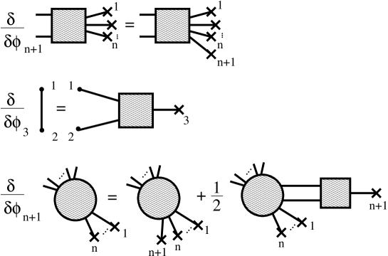
Figure 6: Rules for obtaining the diagrammatic representation of proper vertices: A field derivative can act on three different objects, the self-energy $\bar{\Sigma}(\phi)$, the propagator ${\bar{G}}(\phi)$ and the various derivatives of $i\Gamma_{\rm int}$ represented by circles. The first rule represents the fact that, by definition, adding a leg with a cross to a square box corresponds to taking a derivative with respect to the field. The second rule essentially corresponds to Eq. (2.15). Finally the third rule arises from the fact that a given kernel has both an explicit field-dependence and an implicit one through the function ${\bar{G}}(\phi)$. Thus to the usual explicit derivative with respect to the field, one must add an explicit derivative with respect to $G$ convoluted with a total derivative of the function ${\bar{G}}(\phi)$, hence the additional square box.

As emphasized in Eq. (2.18), all these ladder resummations are generated by the kernel

$$\bar{\Lambda}_{12,34}\equiv 4\frac{\delta^{2}\Gamma_{\mbox{\scriptsize int}}}{\delta G_{12}\delta G_{34}}\Big{|}_{{\bar{G}}}\,.$$ (2.19)

It is therefore useful to introduce the infinite series of ladder graphs, denoted as $\bar{V}_{12,34}$, which satisfies the following integral, Bethe-Salpeter–like equation:

$$\bar{V}_{12,34}=\bar{\Lambda}_{12,34}+\frac{i}{2}\,\bar{\Lambda}_{12,ab}\,{\bar{G}}_{ac}{\bar{G}}_{db}\,\bar{V}_{cd,34}\,.$$ (2.20)

In terms of this vertex-function the set of integral equations (2.18) (cf. also Eq. (2.17)) can be solved explicitly:

$$\frac{\delta^{p}\bar{\Sigma}_{ab}}{\delta\phi_{1}\cdots\delta\phi_{p}}=\mathcal{A}^{ab}_{1\ldots p}+\frac{i}{2}\,\bar{V}_{ab,cd}\,{\bar{G}}_{ce}{\bar{G}}_{fd}\,\mathcal{A}^{ef}_{1\ldots p}\,.$$ (2.21)

When expressed in terms of $\bar{V}$, the $n$-point functions (2.11) only involve a finite number of contributions. This considerably simplifies the analysis of UV singularities.

2.3 Vertex functions for vanishing field expectation value

In the following we present some relevant equations for $\bar{\phi}\equiv 0$, since for the purpose of renormalization it is sufficient to consider the symmetric phase (see Sec. 5). To be explicit, we specify the above general considerations to a four-dimensional $Z_{2}$-symmetric theory with $\varphi^{4}$-interaction. As a consequence all functions made of an odd number of field derivatives of the 2PI effective action vanish. We will make frequent use of the symmetry properties $G_{12}=G_{21}$, $\bar{\Lambda}_{12,34}=\bar{\Lambda}_{21,34}=\bar{\Lambda}_{12,43}=\bar{\Lambda}_{34,12}$ (cf. Eq. (2.19)) and equivalently for the vertex-function $\bar{V}_{12,34}$ given in Eq. (2.20). The two- and four-point functions then read:

$$\Gamma^{(2)}_{12} = iG_{0,12}^{-1}+\frac{\delta^{2}\Gamma_{\mbox{\scriptsize int}}}{\delta\phi_{1}\delta\phi_{2}}\Big{|}_{{\bar{G}}}\,,$$ (2.22)

$$\Gamma^{(4)}_{1234} = \frac{\delta^{4}\Gamma_{\mbox{\scriptsize int}}}{\delta\phi_{1}\cdots\delta\phi_{4}}\Big{|}_{{\bar{G}}}+\left(\frac{\delta^{3}\Gamma_{\mbox{\scriptsize int}}}{\delta\phi_{1}\delta\phi_{2}\delta G_{ab}}\Big{|}_{{\bar{G}}}\,{\bar{G}}_{ac}{\bar{G}}_{db}\,\frac{\delta^{2}\bar{\Sigma}_{cd}}{\delta\phi_{3}\delta\phi_{4}}+{\rm perm.}\right)\,,$$

where ’perm.’ denotes possibe permutations of the indices $(2,3,4)$. The second derivative of the self-energy appearing on the RHS of Eq. (2.3) satisfies the integral equation

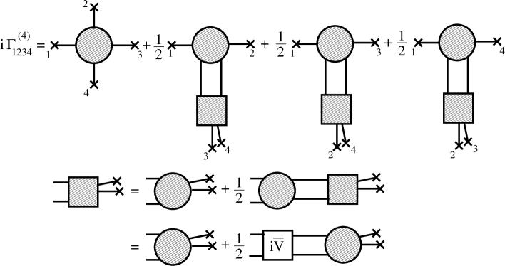
Figure 7: Diagrammatic representation of the fourth derivative of the resummed 2PI effective action in the symmetric phase. It involves the function $\delta^{2}\bar{\Sigma}/\delta\phi^{2}$ which equation can be solved in terms of $\bar{V}$.

$$\frac{\delta^{2}\bar{\Sigma}_{12}}{\delta\phi_{3}\delta\phi_{4}}=\frac{2i\delta^{3}\Gamma_{\mbox{\scriptsize int}}}{\delta G_{12}\delta\phi_{3}\delta\phi_{4}}\Big{|}_{{\bar{G}}}+\frac{i}{2}\bar{\Lambda}_{12,ab}\,{\bar{G}}_{ac}{\bar{G}}_{db}\,\frac{\delta^{2}\bar{\Sigma}_{cd}}{\delta\phi_{3}\delta\phi_{4}}\,.$$ (2.24)

This equation is the one depicted in Fig. 5 for the symmetric phase, where $\bar{\phi}=0$. Equations (2.3) and (2.24) are represented in Fig. 7. As described above, the integral equation (2.24) can be solved explicitely in terms of the vertex-function $\bar{V}$ (cf. Eq. (2.20) and Fig. 7):

$$\frac{\delta^{2}\bar{\Sigma}_{12}}{\delta\phi_{3}\delta\phi_{4}}=\frac{2i\delta^{3}\Gamma_{\mbox{\scriptsize int}}}{\delta G_{12}\delta\phi_{3}\delta\phi_{4}}\Big{|}_{{\bar{G}}}+\frac{i}{2}\,\bar{V}_{12,ab}\,{\bar{G}}_{ac}{\bar{G}}_{db}\,\frac{2i\delta^{3}\Gamma_{\mbox{\scriptsize int}}}{\delta G_{cd}\delta\phi_{3}\delta\phi_{4}}\Big{|}_{{\bar{G}}}\,.$$ (2.25)

Inserting this expression in Eq. (2.3) for the four-point function, one obtains a closed expression in terms of $\bar{V}$ and 2PI kernels. This is represented in Fig. 8 (cf. also Eq. (2.3) below).

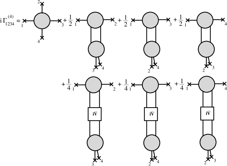
Figure 8: Diagrammatic representation of the fourth derivative of the resummed 2PI effective action in the symmetric phase.

In order to summarize the set of relevant equations to be used in the following, we define:

$$\Sigma_{12}\equiv i\frac{\delta^{2}\Gamma_{\mbox{\scriptsize int}}}{\delta\phi_{1}\delta\phi_{2}}\Big{|}_{{\bar{G}}}\,,$$ (2.26)

as well as

$$\Lambda_{12,34}\equiv 2\frac{\delta^{3}\Gamma_{\mbox{\scriptsize int}}}{\delta\phi_{1}\delta\phi_{2}\delta G_{34}}\Big{|}_{{\bar{G}}}\,,$$ (2.27)

with symmetry properties $\Lambda_{12,34}=\Lambda_{21,34}=\Lambda_{12,43}$. In analogy with the vertex function $\bar{V}$, we introduce the notation:

$$V_{12,34}\equiv-i\frac{\delta^{2}\bar{\Sigma}_{34}}{\delta\phi_{1}\delta\phi_{2}}\,.$$ (2.28)

Leaving space-time indices implicit, the integral equation (2.20) takes the following compact form:

$$\bar{V}=\bar{\Lambda}+\frac{i}{2}\,\bar{\Lambda}\,{\bar{G}}^{2}\,\bar{V}=\bar{\Lambda}+\frac{i}{2}\,\bar{V}\,{\bar{G}}^{2}\,\bar{\Lambda}\,,$$ (2.29)

where the second equality follows from the symmetry properties of the functions $\bar{\Lambda}$ and $\bar{V}$. Similarly, the integral equation (2.24) and its solution (2.25) in terms of $\bar{V}$ now read:

$$V=\Lambda+\frac{i}{2}\,V\,{\bar{G}}^{2}\,\bar{\Lambda}=\Lambda+\frac{i}{2}\,\Lambda\,{\bar{G}}^{2}\,\bar{V}\,.$$ (2.30)

It is important to realize that all the quantities we define are, up to an overall factor, made of a resummation of perturbative diagrams, with no extra factors other than the standard symmetry factors. This is useful in order to discuss renormalization in a diagrammatic way. Finally, it is useful to define the functions $\Lambda^{\dagger}$ and $V^{\dagger}$, such that $\Lambda^{\dagger}_{12,34}\equiv\Lambda_{34,12}$ and similarly for $V^{\dagger}$.

With these notations, the two- and four-point functions read:

$$\Gamma^{(2)} = iG_{0}^{-1}-i\Sigma\,,$$ (2.31)

$$\Gamma^{(4)} = \frac{\delta^{4}\Gamma_{\mbox{\scriptsize int}}}{\delta\phi^{4}}\Big{|}_{{\bar{G}}}+\frac{i}{2}\,\Big{(}\Lambda\,{\bar{G}}^{2}\,V^{\dagger}+{\rm perm.}\Big{)}\,.$$ (2.32)

Using the explicit expression of the function $V$, Eq. (2.30), the four-point function is given by (cf. Fig. 8):

$$\Gamma^{(4)}=\frac{\delta^{4}\Gamma_{\mbox{\scriptsize int}}}{\delta\phi^{4}}\Big{|}_{{\bar{G}}}+\frac{i}{2}\,\Big{(}\Lambda\,{\bar{G}}^{2}\,\Lambda^{\dagger}+\frac{i}{2}\,\Lambda\,{\bar{G}}^{2}\,\bar{V}\,{\bar{G}}^{2}\,\Lambda^{\dagger}+{\rm perm.}\Big{)}\,.\\$$

As emphasized previously, we are left with closed expressions involving only 2PI kernels and the vertex function $\bar{V}$, appearing in a finite number of loop integrals. The same is true for higher $n$-point functions as well. This property will simplify considerably the discussion of renormalization in the next sections.

We point out that a simplification occurs for approximations where the following relation between two-point 2PI kernels is satisfied:

$$\frac{\delta^{2}\Gamma_{\mbox{\scriptsize int}}}{\delta\phi_{1}\delta\phi_{2}}\Big{|}_{\phi=0}=2\frac{\delta\Gamma_{\mbox{\scriptsize int}}}{\delta G_{12}}\Big{|}_{\phi=0}\,.$$ (2.33)

As shown in Appendix LABEL:sec:appcorrel, this implies, in particular, that $\bar{\Sigma}=\Sigma$, $\bar{\Lambda}=\Lambda$ and, consequently, $\bar{V}=V$. Using the integral equation (2.29), the expressions (2.31) and (2.32) for the two- and four-point functions simplify to:

$$\Gamma^{(2)} = i{\bar{G}}^{-1}\,,$$ (2.34)

$$\Gamma^{(4)} = \frac{\delta^{4}\Gamma_{\mbox{\scriptsize int}}}{\delta\phi^{4}}\Big{|}_{{\bar{G}}}+\Big{(}\bar{V}-\bar{\Lambda}+{\rm perm.}\Big{)}\,.$$ (2.35)

Obviously, the renormalization of $\Gamma^{(2)}$ and $\Gamma^{(4)}$ is greatly simplified in that case.

Finally, we mention that in the exact theory, the various two- and four-point functions introduced above satisfy the relations: $\Gamma^{(2)}=i{\bar{G}}^{-1}$ and $\bar{V}=V=\Gamma^{(4)}$, as shown in Appendix LABEL:sec:appcorrel. Although such relations are generally not respected anymore once approximations are introduced, they are important when imposing renormalization conditions as is discussed below.

3 Renormalization

The diagrammatic tools introduced in the previous section allow one to analyze the origin of UV divergences in a very efficient way. As exemplified in Fig. 4 for the case of the three-point function, all diagrammatic contributions to a given proper vertex share a common generic structure: They involve particular 2PI kernels (represented by circles) and field derivatives of the self-energy $\bar{\Sigma}$ (represented by boxes), which enter loops with lines associated to the two-point function ${\bar{G}}$. The 2PI kernels, self-energy derivatives and ${\bar{G}}$ generally contain divergences. Furthermore, the loops they enter may also be divergent. Our renormalization program thus aims at making kernels, self-energy derivatives and ${\bar{G}}$ finite and at removing the remaining divergences in the loop integrals involving these objects. In order to do so, we make extensive use of the techniques put forward in Refs. [16, 17], where the BPHZ subtraction procedure is applied to 2PI diagrams with lines associated to the resummed two-point function ${\bar{G}}$. As a consequence of the two-particle irreducibility of the diagrams, this “2PI” BPHZ analysis automatically gives the correct mass and field-strength counterterms. Moreover, it enables one to identify the counterterms needed to renormalize all kernels $\delta^{m+2n}\Gamma_{\mbox{\scriptsize int}}/\delta G^{m}\delta\phi^{2n}|_{\bar{G}}$ with $2(m+n)\geq 4$ external legs. The two-point kernels $\delta\Gamma_{\mbox{\scriptsize int}}/\delta G|_{\bar{G}}$ and $\delta^{2}\Gamma_{\mbox{\scriptsize int}}/\delta\phi^{2}|_{\bar{G}}$, however, require a more careful analysis: In contrast to standard perturbation theory, the BPHZ procedure applied to resummed diagrams actually misses an infinite number of coupling sub-divergences hidden in the resummed two-point function ${\bar{G}}$. This problem was investigated in detail in Refs. [16, 17] for the case of the kernel $\delta\Gamma_{\mbox{\scriptsize int}}/\delta G|_{\bar{G}}$ in the symmetric phase. There, it has been shown that the hidden sub-divergences are all generated by successive iterations of the Bethe-Salpeter–type equation (2.29) and that they can in fact be absorbed in the renormalization of the function $\bar{V}$. This in turn amounts to a single subtraction, which corresponds to an infinite shift of the tree-level contribution to $\delta^{2}\Gamma_{\mbox{\scriptsize int}}/\delta G^{2}|_{\bar{G}}$, i.e. to a simple coupling counterterm. Here, we apply a similar analysis to the kernel $\delta^{2}\Gamma_{\mbox{\scriptsize int}}/\delta\phi^{2}|_{\bar{G}}$. We show that the corresponding coupling sub-divergences are in fact generated by successive iterations of the integral equation (2.30) and can be absorbed by a shift of the tree-level contribution to the four-point kernel $\delta^{3}\Gamma_{\mbox{\scriptsize int}}/\delta G\delta\phi^{2}|_{\bar{G}}$. This nonperturbative shift renormalizes the function $V$.

Once the two-point kernels have been renormalized, a careful analysis of the expressions derived in the previous section for proper vertices reveals that all potential sub-divergences in the latter can be absorbed in the renormalization of the four-point functions $\bar{V}$ and $V$ and of 2PI kernels with two, six, or more than six legs. In fact, after the latter have been made finite, there remains only an overall divergence in the four-point function $\Gamma^{(4)}$, which can be eliminated by a standard counterterm. The latter corresponds to a shift of the tree-level contribution to the third four-point 2PI kernel $\delta^{4}\Gamma_{\mbox{\scriptsize int}}/\delta\phi^{4}|_{\bar{G}}$. The remarkable result is that the only modifications to the 2PI BPHZ analysis described above reduce to a redefinition of the tree-level contributions to each of the four-point 2PI kernels $\delta^{2}\Gamma_{\mbox{\scriptsize int}}/\delta G^{2}|_{\bar{G}}$, $\delta^{3}\Gamma_{\mbox{\scriptsize int}}/\delta G\delta\phi^{2}|_{\bar{G}}$ and $\delta^{4}\Gamma_{\mbox{\scriptsize int}}/\delta\phi^{4}|_{\bar{G}}$. This is the main result of the present paper. With these counterterms being determined, all proper vertices $\Gamma^{(n)}$ are finite. Furthermore, the zero-point function is finite up to an irrelevant field-independent constant [16].

3.1 Counterterms

We consider a quantum field theory with classical action

$$S[\varphi]=-\int_{x}\,\left\{\frac{1}{2}\,\varphi\left(\square+m^{2}\right)\varphi+\frac{\lambda}{4!}\varphi^{4}\right\}\,,$$ (3.36)

employing the notation $\int_{x}\equiv\int_{\Lambda}d^{4}x$, where the subscript $\Lambda$ refers to some given regularization procedure such as, for instance, cutoff or dimensional regularization. Introducing the renormalized field

$$\varphi_{R}=Z^{-1/2}\varphi\,,$$ (3.37)

the action reads:

$$S[\varphi_{R}] = -\int_{x}\,\left\{\frac{1}{2}\,\varphi_{R}\left(\square+m_{R}^{2}\right)\varphi_{R}+\frac{\lambda_{R}}{4!}\varphi_{R}^{4}\right.$$ (3.38)

$$\left.\hskip 28.45274pt+\,\frac{1}{2}\,\varphi_{R}\left(\delta Z\,\square+\delta m^{2}\right)\varphi_{R}+\frac{\delta\lambda}{4!}\varphi_{R}^{4}\right\},$$

with the standard definitions

$$\delta Z = Z-1\,,$$

$$Zm^{2} = m_{R}^{2}+\delta m^{2}\,,$$ (3.39)

$$Z^{2}\lambda = \lambda_{R}+\delta\lambda\,.$$

Including the counterterms $\sim\delta Z$, $\delta m^{2}$ and $\delta\lambda$ into the interaction part of the action, we define

$$S_{0R}[\varphi_{R}]=-\frac{1}{2}\,\int_{x}\,\varphi_{R}\left(\square+m_{R}^{2}\right)\varphi_{R}\equiv\frac{1}{2}\,\int_{xy}\,\varphi_{R}(x)iG_{0R}^{-1}(x,y)\varphi_{R}(y)\,,$$ (3.40)

where $G_{0R}$ denotes the renormalized free propagator. It follows with Eq. (2.4) that

$$ZG_{0}^{-1}=G_{0R}^{-1}+\delta G_{0}^{-1}\,,$$ (3.41)

where we introduced the notation

$$i\delta G_{0}^{-1}(x,y)=-(\delta Z\,\square+\delta m^{2})\,\delta^{4}(x-y)\,.$$ (3.42)

The corresponding 2PI effective action in terms of the fields $\phi$ and $G$ is given by Eq. (2.5). In terms of the renormalized fields

$$\phi_{R}=Z^{-1/2}\phi\quad,\quad G_{R}=Z^{-1}G\,,$$ (3.43)

it can be written, up to an irrelevant constant, as

$$\Gamma_{\mbox{\scriptsize 2PI}}[\phi_{R},G_{R}] = S_{0R}[\phi_{R}]+\frac{i}{2}\,\hbox{Tr }\ln G_{R}^{-1}+\frac{i}{2}\,\hbox{Tr }G_{0R}^{-1}G_{R}$$ (3.44)

$$+\Gamma_{\mbox{\scriptsize int}}^{R}[\phi_{R},G_{R};\lambda_{R}+\delta\lambda,\delta Z,\delta m^{2}]\,,$$

where we defined the “interaction” functional $\Gamma_{\mbox{\scriptsize int}}^{R}$ in terms of renormalized fields as (note that $\delta G_{0}^{-1}$ is treated as part of the interaction):

$$\Gamma_{\mbox{\scriptsize int}}^{R}[\phi_{R},G_{R};\lambda_{R}+\delta\lambda,\delta Z,\delta m^{2}] = \frac{i}{2}\,\int_{xy}\,\phi_{R}(x)\delta G_{0}^{-1}(x,y)\phi_{R}(y)$$

$$+\frac{i}{2}\,\hbox{Tr }\!\delta G_{0}^{-1}G_{R}+\Gamma_{\mbox{\scriptsize int}}[\phi_{R},G_{R};\lambda_{R}+\delta\lambda]\,.$$

Here, we have used the fact that

$$\Gamma_{\mbox{\scriptsize int}}[\phi,G;\lambda]=\Gamma_{\mbox{\scriptsize int}}[\phi_{R},G_{R};\lambda_{R}+\delta\lambda]\,,$$ (3.46)

which follows from the standard relation between the number of vertices $v$ and the number of external and internal lines, $e$ and $i$, of a given diagram: $4v=e+2i$. Alternatively, one can construct the 2PI effective action in terms of renormalized fields directly from the defining functional integral with action (3.38), treating the counterterms as part of the interaction. The coupling counterterm merely shifts the coupling constant to be used in the vertices of 2PI diagrams whereas the quadratic counterterms $\delta Z$ and $\delta m^{2}$ give new (two-legs) vertices. There are only two 2PI diagrams one can construct with such vertices, which are represented in Fig. 9. These correspond to the first two terms on the RHS of Eq. (LABEL:eq:gammaint_ren).

Figure 9: Diagrammatic representation of the mass and field-strength counterterms. The black dots denote indistinctly the mass counterterm $\delta m^{2}$ or field-strength counterterm $\delta Z$ appearing in the first two terms on the RHS of Eq. (LABEL:eq:gammaint_ren). The line of the closed loop represents $G_{R}$, while a circled cross denotes $\phi_{R}$.

3.2 Conditions for renormalizability

As for perturbative renormalizability, 2PI approximations are typically only renormalizable for systematic expansions. In such cases, each new order of the expansion involves a new selective summation of an infinite series of perturbative contributions and it is non-trivial that such approximations turn out to be renormalizable order by order. There may also be cases where a suitable expansion parameter is missing and one would like to retain only specific 2PI diagrams while dropping others. In this subsection, we give a set of necessary conditions which any 2PI approximation has to fulfill in order to be renormalizable. We will see in the next subsection that these necessary conditions are actually sufficient.

For this it is useful to write $\Gamma_{\mbox{\scriptsize int}}^{R}[\phi_{R},G_{R}]$ as a power series in $\phi_{R}$:

$$\Gamma_{\mbox{\scriptsize int}}^{R}[\phi_{R},G_{R}] = \Gamma_{\mbox{\scriptsize int}}^{(0)}[G_{R}]+\sum_{n=1}^{\infty}\frac{1}{(2n)!}\int_{x_{1},\ldots,x_{2n}}\,\Gamma_{\mbox{\scriptsize int}}^{(2n)}(x_{1},\ldots,x_{2n};G_{R})\,$$ (3.47)

$$\times\,\phi_{R}(x_{1})\cdots\phi_{R}(x_{2n})\,,$$

with zero-field part $\Gamma_{\mbox{\scriptsize int}}^{(0)}[G_{R}]\equiv\Gamma_{\mbox{\scriptsize int}}^{R}[\phi_{R}=0,G_{R}]$ and where

$$\Gamma_{\mbox{\scriptsize int}}^{(2n)}(x_{1},\ldots,x_{2n};G_{R})\equiv\left.\frac{\delta^{2n}\Gamma_{\mbox{\scriptsize int}}^{R}[\phi_{R},G_{R}]}{\delta\phi_{R}(x_{1})\cdots\delta\phi_{R}(x_{2n})}\right|_{\phi_{R}=0}\,.$$ (3.48)

The number of fields is even because of the $Z_{2}$-symmetry of the $\varphi^{4}$-theory.

If $\Gamma_{\mbox{\scriptsize int}}^{(2n)}(G_{R})$ is finite, all the kernels generated from it by taking derivatives with respect to $G_{R}$ are automatically finite. In Fig. 10 we display possible contribution to each of the $\Gamma_{\mbox{\scriptsize int}}^{(2n)}$ for illustration, with the notation introduced in the caption of Fig. 9 for mass and field-strength counterterms. We will consider in the following the minimal requirements for a given approximation (ensemble of graphs) to be renormalizable. A necessary condition is that, whenever a graph contains a potentially divergent sub-diagram, there must be a corresponding graph in the truncation where the divergent sub-diagram has been replaced by a point. The latter corresponds to the counterterm (or BPHZ subtraction) needed to cancel the sub-divergence.

Figure 10: Examples of approximations for $\Gamma_{\mbox{\scriptsize int}}^{(2n)}(G_{R})$, see Eq. (3.47), for $n=0,1,2,3$.

We first discuss two-point singularities. Following the standard procedure, we graphically represent sub-divergences by boxes surrounding the corresponding sub-diagrams. Because of the two-particle irreducibility of the diagrams (see Appendix LABEL:2PItop) for the zero-field part $\Gamma_{\mbox{\scriptsize int}}^{(0)}$ the only two-point boxes one can draw are those which contain all the lines of the diagram but one. As illustrated in Fig. 11, there is one diagram to absorb all these structures. It is given by the first diagram in Fig. 9, which precisely corresponds to mass and field-strength counterterms. We denote the latter by $\delta m^{2}_{0}$ and $\delta Z_{0}$ to emphasize that they arise from the analysis of the zero-field part $\Gamma_{\mbox{\scriptsize int}}^{(0)}$. Similarly, for a given diagram with two external fields, which contributes to $\Gamma_{\mbox{\scriptsize int}}^{(2)}$, the only possible two-point box one can draw is the one containing the whole graph.

Figure 11: Illustration for the analysis of two-point singularities. The factors arise from the different possibilities to draw a two-point box.

The associated divergences can be absorbed in the mass and field-strength counterterms represented by the second diagram in Fig. 9. We denote the latter by $\delta m^{2}_{2}$ and $\delta Z_{2}$. We emphasize that for a given truncation these are not necessarily the same as $\delta m^{2}_{0}$ and $\delta Z_{0}$, which just reflects the fact that these are different approximations of the same counterterm (cf. below). Finally, there are no two-point boxes in 2PI diagrams with more than two external fields ($\Gamma_{\mbox{\scriptsize int}}^{(2n)}$ with $n\geq 2$) for precisely the same topological reasons as there can be no other graphs than those of Fig. 9 with mass and field-strength counterterms. This in turn is related to the fact that the latter only arise in the renormalization of the two-point 2PI kernels $\delta\Gamma_{\mbox{\scriptsize int}}^{R}/\delta G_{R}|_{{\bar{G}}_{R}}$ and $\delta^{2}\Gamma_{\mbox{\scriptsize int}}^{R}/\delta\phi_{R}^{2}|_{{\bar{G}}_{R}}$.

We now turn to four-point singularities. If a given loop diagram is included in the truncation, all topologies generated by the BPHZ procedure described above must be included as well. Note that the latter only generates topologies with lower number of loops. For instance, if the three-loop (basket-ball) diagram is included, one needs to include the two-loop (eight) diagram as well. Similarly, the renormalization of the two-loop diagram with two external fields (setting-sun) requires the presence of the one-loop diagram with two external fields (tadpole) in the truncation. This is illustrated in Fig. 12. We note that this procedure does not mix diagrams with different number of external fields and can therefore be applied to each of the $\Gamma_{\mbox{\scriptsize int}}^{(2n)}$ separately.

Figure 12: Diagrammatic analysis of four-point singularities. The factors arise from the different possibilities to draw a four-point box.

It turns out that this simple analysis gives the relevant subtractions needed to renormalize all 2PI kernels $\delta^{m+2n}\Gamma_{\mbox{\scriptsize int}}^{R}/\delta G_{R}^{m}\delta\phi_{R}^{2n}|_{{\bar{G}}_{R}}=\delta^{m}\Gamma_{\mbox{\scriptsize int}}^{(2n)}/\delta G_{R}^{m}|_{{\bar{G}}_{R}}$ having a number of legs $2(n+m)\geq 4$.

The case of two-point kernels given in Eqs. (2.8) and (2.26) is, however, more subtle and requires special attention. Indeed, drawing boxes on 2PI diagrams misses an infinite number of coupling sub-divergences which arise for $G_{R}={\bar{G}}_{R}$ at the stationary point of the effective action as illustrated in Fig. 13. The case of the two-point kernel

$$\bar{\Sigma}_{R}=2i\frac{\delta\Gamma_{\mbox{\scriptsize int}}^{(0)}}{\delta G_{R}}\Big{|}_{{\bar{G}}_{R}}\,,$$ (3.49)

has been analyzed in detail in Refs. [16, 17]. There, it has been shown that these coupling singularities precisely correspond to those of the Bethe-Salpeter–type equation (2.29) and that they can be absorbed in a shift of the tree-level contribution to the four-point kernel (2.19). Denoting this local shift by $\Delta\lambda_{0}$, we write:

$$4\frac{\delta^{2}\Gamma_{\mbox{\scriptsize int}}^{(0)}}{\delta G_{R}^{2}}\Big{|}_{{\bar{G}}_{R}}\equiv Z^{2}\bar{\Lambda}=\bar{\Lambda}_{R}-\Delta\lambda_{0}\,.$$ (3.50)

where $Z$ is the wave-function renormalization introduced in Eq. (3.37). The function $\bar{\Lambda}_{R}$ is made finite by the previous 2PI BPHZ analysis. The local shift $\Delta\lambda_{0}$ arises from a single graph in the 2PI expansion of the zero-field contribution $\Gamma_{\mbox{\scriptsize int}}^{(0)}[G_{R}]$ in Eq. (3.47), namely the two-loop (eight) diagram. It contributes to the corresponding counterterm, which we denote by $\delta\lambda_{0}$, and adds to the contribution $\delta\lambda_{0}^{\rm BPHZ}$ arising from the BPHZ analysis described previously (see Fig. 12). One has:

$$\delta\lambda_{0}=\delta\lambda_{0}^{\rm BPHZ}+\Delta\lambda_{0}\,.$$ (3.51)

Successive iterations of the kernel (3.50) through the Bethe-Salpeter–type equation (2.29) define a finite four-point function $\bar{V}_{R}=Z^{2}\bar{V}$. This is actually sufficient to show that the coupling divergences hidden in the kernel $\bar{\Sigma}_{R}$ have been removed by the subtraction employed in Eq. (3.50) [16, 17]. An illustration of this is given in Fig. 14.

Figure 13: The BPHZ procedure applied to diagrams with resummed propagators misses singularities. This is simply because the two operations “drawing boxes” (1) and “iterating diagrams” (2) do not commute as illustrated in the figure for the case of the self-energy (3.49). The first line shows the coupling singularities which are accounted for by the BPHZ analysis regardless of the content of the propagator. The second line shows what happens if one first iterates the resummed propagator and then apply the BPHZ analysis. There are clearly more divergent topologies in the second case.

A similar analysis can be applied to the two-point kernel (2.26) which is obtained from the two-field part $\Gamma_{\mbox{\scriptsize int}}^{(2)}(G_{R})$ in the decomposition (3.47) as

$$\Sigma_{R}=i\Gamma_{\mbox{\scriptsize int}}^{(2)}({\bar{G}}_{R})\,.$$ (3.52)

As before, the perturbative expansion of this equation generates coupling singularities which were not taken into account by the previous BPHZ analysis applied to resummed diagrams. Expanding the resummed propagator in terms of perturbative contributions in Eq. (3.52), one observes that these singularities actually correspond to those generated by the integral equation (2.30). By drawing all possible four-point boxes, one sees that part of these singularities actually correspond to those discussed previously for the renormalization of the function $\bar{V}_{R}$ and are, therefore, absorbed in the counterterm $\delta\lambda_{0}$. This is illustrated in Fig. 15. The remaining singularities all have the topology of the tadpole contribution to $\Gamma_{\mbox{\scriptsize int}}^{(2)}(G_{R})$, as illustrated in Fig. 16.

Figure 14: The coupling divergences in the two-point kernel $\delta\Gamma_{\mbox{\scriptsize int}}/\delta G$ are those of the function $\bar{V}$. The total counterterm $\delta\lambda_{0}=\delta\lambda_{0}^{\rm BPHZ}+\Delta\lambda_{0}$ accounts for the divergences of the four-point kernel $\delta^{2}\Gamma_{\mbox{\scriptsize int}}^{R}/\delta G_{R}^{2}|_{{\bar{G}}_{R}}$ ($\delta\lambda_{0}^{\rm BPHZ}$) and the divergences generated by superposing kernels through the integral Bethe-Salpeter–type equation for $\bar{V}_{R}$ ($\Delta\lambda_{0}$).

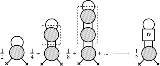
Figure 15: Illustration of the part of the four-point singularities in $\Gamma_{\mbox{\scriptsize int}}^{(2)}(G_{R})$, which is already taken into account in the renormalization of $\bar{V}_{R}$.

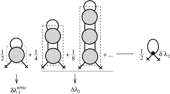
Figure 16: Illustration of the fact that the remaining singularities can all be accounted for by the counterterm $\delta\lambda_{2}=\delta\lambda_{2}^{\rm BPHZ}+\Delta\lambda_{2}$. The latter arises from the tadpole diagram in the 2PI effective action.

They may therefore be absorbed in the corresponding counterterm $\delta\lambda_{2}$. We denote the corresponding contribution by $\Delta\lambda_{2}$. In complete analogy with the previous case, this corresponds to a redefinition of the tree-level contribution to the four-point kernel (2.27):

$$2\frac{\delta\Gamma_{\mbox{\scriptsize int}}^{(2)}}{\delta G_{R}}\Big{|}_{{\bar{G}}_{R}}\equiv Z^{2}\Lambda=\Lambda_{R}-\Delta\lambda_{2}\,.$$ (3.53)

where the function $\Lambda_{R}$ is finite thanks to the 2PI BPHZ analysis. Similarly as before, the shift $\Delta\lambda_{2}$ gives a contribution to the counterterm $\delta\lambda_{2}$ associated with the tadpole contribution to $\Gamma_{\mbox{\scriptsize int}}^{(2)}(G_{R})$, which adds to the contribution $\delta\lambda_{2}^{\rm BPHZ}$ arising from the BPHZ analysis applied to resummed diagrams:

$$\delta\lambda_{2}=\delta\lambda_{2}^{\rm BPHZ}+\Delta\lambda_{2}\,.$$ (3.54)

In the following, we show that the kernels (3.50) and (3.53) define a finite four-point function $V_{R}=Z^{2}V$ through the integral equation (2.30) and that all coupling sub-divergences of the two-point kernel (3.52) can indeed be absorbed in the renormalization of the functions $\bar{V}_{R}$ and $V_{R}$. The remaining overall divergences are absorbed in the mass and field-strength counterterms $\delta m^{2}_{2}$ and $\delta Z_{2}$.

It is remarkable that the previous analysis is almost all what is needed for the renormalization for the 2PI-resummed effective action (2.10). For instance, it is already clear from Eq. (2.22) that the second derivative or two-point function is finite. However, one observes that the loop integrals in Eq. (2.32) together with the successive iterations of Eq. (2.30) bring a priori infinitely many new divergences. The same holds for all higher $n$-point functions. We will show below that all potential sub-divergences can in fact be absorbed in the renormalization of 2PI kernels with two, six, or more than six legs, and of the four-point functions $\bar{V}_{R}$ and $V_{R}$. The only remaining singularity is a global divergence of the four-point vertex function (2.32), which can be absorbed in a contribution $\Delta\lambda_{4}$ to the counterterm $\delta\lambda_{4}$ associated with the tree-level contribution to the four-point kernel

$$\frac{\delta\Gamma_{\mbox{\scriptsize int}}^{R}}{\delta\phi_{R}^{4}}\Big{|}_{{\bar{G}}_{R}}=\Gamma_{\mbox{\scriptsize int}}^{(4)}({\bar{G}}_{R})\,.$$ (3.55)

To summarize, we have seen that a first condition for renormalizability is that for each 2PI graph included in the approximation all topologies generated by the BPHZ procedure described above (i.e., drawing all possible four-point boxes and replacing them by a point) must be included as well. In addition, one must include an infinite shift of the tree-level contribution to the four-point kernels (3.50), (3.53) and (3.55). At the level of the 2PI functional, this corresponds to an infinite shift of the contributions from each local, mass-dimension four operator. To make this explicit, we write:

$$\Gamma_{\mbox{\scriptsize int}}^{R}[\phi_{R},G_{R}] = \gamma_{\mbox{\scriptsize int}}[\phi_{R},G_{R}]-\int_{x}\,\left\{\frac{\Delta\lambda_{0}}{8}\,G_{R}^{2}(x,x)+\frac{\Delta\lambda_{2}}{4}\,G_{R}(x,x)\phi_{R}^{2}(x)\right.$$ (3.56)

$$\hskip 91.04872pt\left.+\frac{\Delta\lambda_{4}}{4!}\,\phi_{R}^{4}(x)\right\}\,.$$

The diagrams corresponding to the shifted part of the 2PI functional are shown in Fig. 17.

Figure 17: Diagrammatic representation of the counterterms needed to renormalize the divergences missed by the BPHZ analysis applied to diagrams with resummed propagators.

Equation (3.56) defines the functional $\gamma_{\mbox{\scriptsize int}}[\phi_{R},G_{R}]$. Employing an equivalent expansion in terms of powers of the field $\phi_{R}$ as in (3.47), the four-point kernels $\delta^{2}\gamma_{\mbox{\scriptsize int}}^{(0)}/\delta G_{R}^{2}|_{{\bar{G}}_{R}}$, $\delta\gamma_{\mbox{\scriptsize int}}^{(2)}/\delta G_{R}|_{{\bar{G}}_{R}}$ and $\gamma_{\mbox{\scriptsize int}}^{(4)}|_{{\bar{G}}_{R}}$, as well as all higher kernels $\delta^{m}\gamma_{\mbox{\scriptsize int}}^{(2n)}/\delta G_{R}^{m}|_{{\bar{G}}_{R}}$ with $n+m>2$ are made finite by the BPHZ subtraction procedure applied to graphs with resummed propagator. For later discussions it is useful to extract the mass and field-strength counterterms explicitely (cf. Eq. (LABEL:eq:gammaint_ren)). Accordingly, we write:

$$\gamma_{\mbox{\scriptsize int}}[\phi_{R},G_{R}] = \tilde{\gamma}_{\mbox{\scriptsize int}}[\phi_{R},G_{R}]-\frac{1}{2}\int_{x}\,\Big{\{}\phi_{R}(x)\left[\delta Z_{0}\square_{x}+\delta m^{2}_{0}\right]\phi_{R}(x)$$ (3.57)

$$+\left[\delta Z_{2}\square_{x}+\delta m^{2}_{2}\right]G_{R}(x,y)|_{y=x}\Big{\}}\,.$$

Section 4 below is devoted to a direct proof that the three counterterms $\Delta\lambda_{0}$, $\Delta\lambda_{2}$ and $\Delta\lambda_{4}$ are actually sufficient to absorb the remaining divergences missed by the 2PI BPHZ procedure and, thereby, to obtain renormalized $n$-point functions from the 2PI-resummed effective action. We show how to compute these counterterms explicitly. We emphasize that, as far as the 2PI BPHZ analysis is concerned, the various $\Gamma_{\mbox{\scriptsize int}}^{(2n)}$ can be treated independently from each other. This is only slightly modified by the complete analysis. In particular, the $\gamma_{\mbox{\scriptsize int}}^{(2n)}$ introduced above remain independent.

3.3 Counterterms and renormalization conditions

We have seen that, in order to renormalize the functions $\bar{V}_{R}$, $V_{R}$ and $\Gamma_{R}^{(4)}$, we need three a priori different coupling counterterms: $\Delta\lambda_{0}$, $\Delta\lambda_{2}$ and $\Delta\lambda_{4}$ respectively. It is important to realize that, although these functions may be different at a given order of approximation, they are in fact not independent in the exact theory, where one has $\bar{V}_{R}=V_{R}=\Gamma_{R}^{(4)}$ (cf. Appendix LABEL:sec:appcorrel). To guarantee that a given approximation scheme converges to the correct theory, it is therefore important to maintain this relation when stating renormalization conditions at each approximation order. For instance, the renormalized coupling $\lambda_{R}$ may be defined at a given renormalization point $\{p_{i}=\tilde{p}_{i}\,,\,i=1,\ldots,4\}$ in Fourier space by:

$$\Gamma_{R}^{(4)}(\tilde{p}_{i})=\bar{V}_{R}(\tilde{p}_{i})=V_{R}(\tilde{p}_{i})=-\lambda_{R}\,.$$ (3.58)

In the following, we will choose the renormalization point in Euclidean momentum space such that $\tilde{p}_{1}=\tilde{p}_{2}=\ldots=\tilde{p}$, with $\tilde{p}^{2}=\mu^{2}$. We stress that Eq. (3.58) expresses a single renormalization condition for the three functions $\bar{V}_{R}$, $V_{R}$ and $\Gamma_{R}^{(4)}$ and uniquely determines the three counterterms $\Delta\lambda_{0}$, $\Delta\lambda_{2}$ and $\Delta\lambda_{4}$. Similarly, the two a priori different sets of field-strength and mass counterterms $(\delta Z_{0},\,\delta m^{2}_{0})$ and $(\delta Z_{2},\,\delta m^{2}_{2})$ are uniquely determined by imposing the same renormalization conditions for the functions $i{\bar{G}}_{R}^{-1}$ and $\Gamma_{R}^{(2)}$, respectively. The latter are equal in the exact theory. For instance, one has:

$$\Gamma_{R}^{(2)}(p=\tilde{p})=i{\bar{G}}_{R}^{-1}(p=\tilde{p})\,\,=\,-m_{R}^{2}$$ (3.59)

$$\frac{d\Gamma_{R}^{(2)}}{dp^{2}}\Big{|}_{p=\tilde{p}}=i\frac{d{\bar{G}}_{R}^{-1}}{dp^{2}}\Big{|}_{p=\tilde{p}}\,=\,-1\,.$$ (3.60)

Finally, we would like to comment on the BPHZ subtraction procedure described previously. It is clear that the latter is equivalent to adding a different counterterm at each vertex appearing in the diagrammatic expansion of the 2PI functional. We stress that these, together with the $\Delta\lambda$’s discussed above actually represent different approximations to one and the same counterterm $\delta\lambda$ introduced in Sec. 3.1. Similarly the field-strength and mass counterterms $(\delta Z_{0},\delta m^{2}_{0})$ and $(\delta Z_{2},\delta m^{2}_{2})$ are two different approximations to $(\delta Z,\delta m^{2})$ introduced before. This is similar to standard perturbation theory, where one would expand the counterterm appearing in each graph to different orders, depending on the order of the graph itself. For practical purposes, this means different counterterms are associated to different graphs. In terms of the BPHZ subtraction scheme, it is crucial that the subtractions are always performed at the same subtraction point. In the present context, the latter should coincide with the renormalization point employed in Eqs. (3.58)–(3.60).

4 Proof

Without loss of generality, the detailed analysis of divergences is most conveniently done in Euclidean Fourier space. Accordingly, we introduce the Euclidean four-momentum $q^{\mu}\equiv(iq_{0},\vec{q})$. We denote the Euclidean integration measure by: $\int_{q}\equiv\int\frac{d^{4}q}{(2\pi)^{4}}$.

4.1 Renormalization of 2PI kernels

As described above, the renormalization of kernels with more than four external legs is based on the BPHZ procedure applied to diagrams with resummed propagator. To illustrate the procedure, we consider the example of the function $\bar{\Lambda}_{R}$ as obtained from the three-loop approximation of the 2PI effective action. After opening two propagator lines to obtain the function $\bar{\Lambda}_{R}$, this corresponds to the one-loop expression represented in Fig. 18. In momentum space this reads:

$$\bar{\Lambda}_{R}(p_{1},\ldots,p_{4})=-\Big{(}\lambda_{R}+\delta\lambda_{0}^{\rm BPHZ}\Big{)}+\lambda_{R}^{2}\int_{q}\,{\bar{G}}_{R}(q){\bar{G}}_{R}(p_{1}+p_{3}+q)\,.$$ (4.61)

The 2PI BPHZ procedure amounts here to choosing $\delta\lambda_{0}^{\rm BPHZ}$ in

Figure 18: The one-loop approximation to the function $\bar{\Lambda}_{R}$, obtained from the 2PI effective action to three loop after cutting two lines, that is after taking two derivatives with respect to $G$. The first two terms arise from the two-loop (eight) diagram whereas the third one comes from the basket-ball diagram. The logarithmic divergence of the third term can be absorbed in the counterterm $\delta\lambda_{0}^{\rm BPHZ}$.

order to renormalize the one-loop integral in Eq. (4.61). With our convention for the renormalization point (cf. Sec. 3.3 above) we choose:

$$\delta\lambda_{0}^{\rm BPHZ}=\lambda_{R}^{2}\int_{q}\,{\bar{G}}_{R}(q){\bar{G}}_{R}(p+q)|_{p^{2}=4\mu^{2}}\,,$$ (4.62)

so that the function

$$\bar{\Lambda}_{R}(p_{1},\ldots,p_{4})=-\lambda_{R}+\lambda_{R}^{2}\int_{q}\,{\bar{G}}_{R}(q)\,\Big{(}{\bar{G}}_{R}(p_{1}+p_{3}+q)-{\bar{G}}_{R}(p+q)|_{p^{2}=4\mu^{2}}\Big{)}$$ (4.63)

is finite. A similar analysis holds for the function $\Lambda_{R}$ as well as for all 2PI kernels with more than four external legs.

As explained in the previous subsection, in order to renormalize the two-point kernels, one first needs to renormalize the vertices $\bar{V}_{R}$ and $V_{R}$, obtained from the integral equations (2.29) and (2.30) respectively. This requires additional contributions $\Delta\lambda_{0}$ and $\Delta\lambda_{2}$ to the counterterms $\delta\lambda_{0}$ and $\delta\lambda_{2}$ respectively, see Eqs. (3.51) and (3.54). We note that due to these additional infinite contributions, the kernels (3.50) and (3.53) are not finite, in contrast to the functions $\bar{\Lambda}_{R}$ and $\Lambda_{R}$. However, this poses no problem for the renormalization program, since these kernels can always be traded for the finite vertices $\bar{V}_{R}$ and $V_{R}$. We make this explicit in the next subsections.

4.1.1 The first vertex-equation

The integral equation (2.29) resums the infinite series of ladder diagrams with rungs given by the kernel (2.19). In terms of renormalized quantities, each iteration brings a new finite rung $\bar{\Lambda}_{R}=4\delta^{2}\gamma_{\mbox{\scriptsize int}}^{(0)}/\delta G_{R}^{2}|_{{\bar{G}}_{R}}$ together with a counterterm $-\Delta\lambda_{0}$. The new logarithmic divergences generated at each iteration can be absorbed in the counterterms appearing in the previous iterations. This is illustrated in Fig. 19.

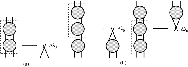
Figure 19: The figures (a) and (b) show the procedure by which the coupling divergences in the vertex equation are absorbed in the shift $\Delta\lambda_{0}$. The overall divergence absorbed at a given iteration is used to remove all the sub-divergences at the next iteration.

Figure 20: The 2PI character of the kernels plays a crucial role in the renormalization of the vertex $\bar{V}_{R}$: There can be no four-point boxes such as the one depicted in the figure. For the same reason, there is no counterterm to absorb such structures.

The 2PI character of the kernel (cf. the discussion in Appendix LABEL:2PItop) prevents other potential divergences to appear (such as the one depicted in Fig. 20). In fact, for precisely the same reason, there is no topology which could be used to cancel such a divergence. This diagrammatic property has its counterpart in the algebraic proof that we now recall [16, 17]. We introduce the notation:

$$\bar{\Lambda}_{R}(p,k)\equiv\bar{\Lambda}_{R}(p,-p,-k,k)\,,$$ (4.64)

where $\bar{\Lambda}_{R}(p_{1},\ldots,p_{4})$ is the Fourier transform of the renormalized function $\bar{\Lambda}_{R}$, as defined from (2.19). One has $\bar{\Lambda}_{R}(p,k)\sim\ln k$ at large $k$ and fixed $p$. Furthermore, it follows from Weinberg’s theorem and from the two-particle irreducible character of the function $\bar{\Lambda}_{R}$, that [16, 17]:

$$\bar{\Lambda}_{R}(p,k)-\bar{\Lambda}_{R}(q,k)\sim\frac{1}{k}\,,$$ (4.65)

at large $k$ and fixed $p$ and $q$. We first consider the vertex equation in the $s$-chanel, namely for the function $\bar{V}_{R}(p,k)\equiv\bar{V}_{R}(p,-p,-k,k)$:

$$\bar{V}_{R}(p,k) = \bar{\Lambda}_{R}(p,k)-\Delta\lambda_{0}+\frac{1}{2}\,\int_{q}\,\bar{V}_{R}(p,q)\,{\bar{G}}_{R}^{2}(q)\,\Big{(}\bar{\Lambda}_{R}(q,k)-\Delta\lambda_{0}\Big{)}$$

$$= \bar{\Lambda}_{R}(p,k)-\Delta\lambda_{0}+\frac{1}{2}\,\int_{q}\,\Big{(}\bar{\Lambda}_{R}(p,q)-\Delta\lambda_{0}\Big{)}\,{\bar{G}}_{R}^{2}(q)\,\bar{V}_{R}(q,k)\,,$$

where we used the fact that $\bar{V}_{R}(p,k)=\bar{V}_{R}(k,p)$, and similarly for $\bar{\Lambda}_{R}(p,k)$. As for $\bar{\Lambda}_{R}(p,k)$, one has $\bar{V}_{R}(p,k)\sim\ln k$ at large $k$ and fixed $p$. This equation contains UV divergent loops but also counterterms. The input of renormalization is simply to state that the value of $\bar{V}_{R}$ at a given renormalization point is finite. For the vertex equation to be self-consistently renormalizable, this has to be enough to obtain a finite equation for $\bar{V}_{R}$. Imposing, as in Eq. (3.58), that $\bar{V}_{R}(\tilde{p},\tilde{p})=-\lambda_{R}$ is finite, we consider the difference:

$$\bar{V}_{R}(p,k)-\bar{V}_{R}(\tilde{p},\tilde{p}) = \bar{\Lambda}_{R}(p,k)-\bar{\Lambda}_{R}(\tilde{p},\tilde{p})$$

$$+\frac{1}{2}\,\int_{q}\,\bar{V}_{R}(p,q)\,{\bar{G}}_{R}^{2}(q)\,\Big{(}\bar{\Lambda}_{R}(q,k)-\bar{\Lambda}_{R}(q,\tilde{p})\Big{)}$$

$$+\frac{1}{2}\,\int_{q}\,\Big{(}\bar{\Lambda}_{R}(p,q)-\bar{\Lambda}_{R}(\tilde{p},q)\Big{)}\,{\bar{G}}_{R}^{2}(q)\,\bar{V}_{R}(q,\tilde{p})\,,$$

where we used the symmetry property of the momentum integral in Eq. (4.1.1) so that only differences of 2PI kernels appear. In this way, all counterterms – which are momentum independent – disappear from this equation. Using the asymptotic behavior (4.65), one easily checks that the integrals in Eq. (4.1.1) are finite.

We also need to consider the full momentum dependence of $\bar{V}_{R}$ which satisfies the following equation, where $\bar{V}_{R}(p,q,k)\equiv\bar{V}_{R}(p,-q,-k,k+q-p)$ and similarly for $\bar{\Lambda}_{R}$:

$$\bar{V}_{R}(p,q,k) = \bar{\Lambda}_{R}(p,q,k)-\Delta\lambda_{0}$$

$$+\frac{1}{2}\,\int_{r}\,\Big{(}\bar{\Lambda}_{R}(p,q,r)-\Delta\lambda_{0}\Big{)}\,{\bar{G}}_{R}(r)\,{\bar{G}}_{R}(l)\,\bar{V}_{R}(r,l,k)\,,$$

where $l=r+q-p$. The divergent part of the momentum integral in the equation above comes from the large $r$ contribution:

$$\bar{V}_{R}(p,q,k)|_{\rm div} = \bar{\Lambda}_{R}(p,q,k)-\Delta\lambda_{0}$$

$$+\frac{1}{2}\,\int_{r}\,\Big{(}\bar{\Lambda}_{R}(p,q,r)-\Delta\lambda_{0}\Big{)}\,{\bar{G}}_{R}^{2}(r)\,\bar{V}_{R}(r,r,k)\,.$$

The latter precisely coincides with the divergences of $\bar{V}_{R}(p,k)=\bar{V}_{R}(p,p,k)$ discussed above. Indeed, one has:

$$\bar{V}_{R}(p,q,k)|_{\rm div}-\bar{V}_{R}(p,p,k)=\bar{\Lambda}_{R}(p,q,k)-\bar{\Lambda}_{R}(p,p,k)$$

$$\qquad\qquad\qquad\qquad\quad+\frac{1}{2}\,\int_{r}\,\Big{(}\bar{\Lambda}_{R}(p,q,r)-\bar{\Lambda}_{R}(p,p,r)\Big{)}\,{\bar{G}}_{R}^{2}(r)\,\bar{V}_{R}(r,r,k)\,,$$

which is finite due to the fact that, as a consequence of two-particle-irreducibility, $\bar{\Lambda}_{R}(p,q,r)-\bar{\Lambda}_{R}(p,p,r)\sim 1/r$ at large $r$ and fixed $p$ and $q$.

4.1.2 Renormalization of $\delta\Gamma_{\mbox{\scriptsize int}}^{R}/\delta G_{R}|_{{\bar{G}}_{R}}$

The renormalization of the kernel $\delta\Gamma_{\mbox{\scriptsize int}}^{R}/\delta G_{R}|_{{\bar{G}}_{R}}$, or equivalently, of the auxiliary propagator ${\bar{G}}_{R}$ has been extensively discussed in Refs. [16, 17]. Here, we briefly recall the main arguments of the analysis. This only involves the zero-field part $\Gamma_{\mbox{\scriptsize int}}^{(0)}[G_{R}]$ of the 2PI effective action. The 2PI BPHZ procedure fixes the counterterms $\delta Z_{0}$, $\delta m^{2}_{0}$, and a set of $\delta\lambda_{0}^{\rm BPHZ}$’s for each topology appearing in the truncation (cf. Sec. 3.3), adjusted so that the four-point kernel $\delta^{2}\gamma_{\mbox{\scriptsize int}}^{(0)}/\delta G_{R}^{2}|_{{\bar{G}}_{R}}$ is finite. The remaining divergences in the two-point kernel $\delta\Gamma_{\mbox{\scriptsize int}}^{R}/\delta G_{R}|_{{\bar{G}}_{R}}$ are made explicit by performing an asymptotic expansion of ${\bar{G}}_{R}$ in its defining equation

$${\bar{G}}_{R}^{-1}=G_{0R}^{-1}-\bar{\Sigma}_{R}({\bar{G}}_{R})\,,$$ (4.71)

with

$$\bar{\Sigma}_{R}({\bar{G}}_{R})=2i\frac{\delta\Gamma_{\mbox{\scriptsize int}}^{R}}{\delta G_{R}}\Big{|}_{{\bar{G}}_{R}}\,.$$ (4.72)

Following Ref. [17], we separate the leading asymptotic behavior $\bar{\Sigma}_{2}(p)\sim p^{2}$ of the self-energy $\bar{\Sigma}_{R}(p)$ at large momentum $p$:

$$\bar{\Sigma}_{R}(p)=\bar{\Sigma}_{2}(p)+\bar{\Sigma}_{0}(p)\,,$$ (4.73)

where the function $\bar{\Sigma}_{0}(p)$ grows at most as powers of $\ln p$ at large $p$. Similarly, we extract the leading asymptotic behavior ${\bar{G}}_{2}(p)\sim 1/p^{2}$ of the propagator ${\bar{G}}_{R}(p)$:

$${\bar{G}}_{R}(p)={\bar{G}}_{2}(p)+\delta{\bar{G}}(p)\,,$$ (4.74)

where the function $\delta{\bar{G}}(p)\sim 1/p^{4}$ at most. One has, explicitly:

$${\bar{G}}_{R}^{-1}(p)=i(p^{2}+m_{R}^{2})-\bar{\Sigma}_{2}(p)-\bar{\Sigma}_{0}(p)$$ (4.75)

and

$${\bar{G}}_{2}^{-1}(p)=ip^{2}-\bar{\Sigma}_{2}(p)\,,$$ (4.76)

from which follows

$$\delta{\bar{G}}(p)={\bar{G}}_{2}(p)\left[-im_{R}^{2}+\bar{\Sigma}_{0}(p)\right]{\bar{G}}_{2}(p)+{\bar{G}}_{r}(p)\,,$$ (4.77)

where ${\bar{G}}_{r}(p)\sim 1/p^{6}$ at most. We now expand the right hand side of Eq. (4.72) according to (4.74). Using

$$\bar{\Sigma}_{2}\equiv\bar{\Sigma}_{R}({\bar{G}}_{2})+i\delta m^{2}_{0}\,,$$ (4.78)

the leading term of the expansion cancels with $\bar{\Sigma}_{2}$ and one obtains, for the sub-leading part

$$\bar{\Sigma}_{0}(p)=-i\delta m^{2}_{0}+\frac{1}{2}\,\int_{q}\Big{(}\bar{\Lambda}_{2}(p,q)-\Delta\lambda_{0}\Big{)}\,\delta{\bar{G}}(q)+\bar{\Sigma}_{r}(p)\,,$$ (4.79)

where $\bar{\Lambda}_{2}\equiv\bar{\Lambda}_{R}({\bar{G}}_{2})$, see Eq. (4.64), and $\bar{\Sigma}_{r}(p)$ is a finite function decreasing at least as $1/p$ at large $p$. It is possible to absorb all the non-localities in a redefinition of $\bar{\Sigma}_{r}(k)$ ($p=\tilde{p}$ denotes the renormalization point):

$$\bar{\Sigma}_{0}(p)=-i\delta m^{2}_{0}+\frac{1}{2}\,\int_{q}\Big{(}\bar{\Lambda}_{2}(\tilde{p},q)-\Delta\lambda_{0}\Big{)}\,\delta{\bar{G}}(q)+\bar{\Sigma}^{\prime}_{r}(p)\,,$$ (4.80)

with

$$\bar{\Sigma}^{\prime}_{r}(p)=\bar{\Sigma}_{r}(p)+\frac{1}{2}\,\int_{q}\Big{(}\bar{\Lambda}_{2}(p,q)-\bar{\Lambda}_{2}(\tilde{p},q)\Big{)}\,\delta{\bar{G}}(q)\,.$$ (4.81)

Indeed, using Weinberg’s theorem and the asymptotic behavior (4.65), one can show that the integral on the RHS of (4.81) is finite and decreases at least as $1/p$ at large $p$. We now use the vertex equation (4.1.1) with propagator ${\bar{G}}_{2}$ – which solution we denote by $\bar{V}_{2}(p,k)$ – to trade $\bar{\Lambda}_{2}(\tilde{p},q)$ for $\bar{V}_{2}(\tilde{p},q)$ in (4.80):

$$\bar{\Sigma}_{0}(p) = -i\delta m^{2}_{0}+\bar{\Sigma}^{\prime}_{r}(p)+\frac{1}{2}\,\int_{q}\,\bar{V}_{2}(\tilde{p},q)\,\delta{\bar{G}}(q)$$ (4.82)

$$-\frac{1}{4}\,\int_{q}\int_{k}\,\bar{V}_{2}(\tilde{p},q)\,{\bar{G}}_{2}^{2}(q)\,\Big{(}\bar{\Lambda}_{2}(q,k)-\Delta\lambda_{0}\Big{)}\,\delta{\bar{G}}(k)\,.$$

Using (4.79), one can rewrite the integral over $k$ in the last term:

$$\bar{\Sigma}_{0}(p) = -i\delta m^{2}_{0}+\bar{\Sigma}^{\prime}_{r}(p)+\frac{1}{2}\,\int_{q}\,\bar{V}_{2}(\tilde{p},q)\,\delta{\bar{G}}(q)$$ (4.83)

$$-\frac{1}{2}\,\int_{q}\,\bar{V}_{2}(\tilde{p},q)\,{\bar{G}}_{2}^{2}(q)\,\Big{\{}\bar{\Sigma}_{0}(q)-\bar{\Sigma}_{r}(q)+i\delta m^{2}_{0}\Big{\}}\,.$$

Using (4.77), one sees that the potentially divergent terms which depend on $\bar{\Sigma}_{0}$ cancel out. One finally obtains

$$\bar{\Sigma}_{0}(p) = \frac{1}{2}\,\int_{q}\,\bar{V}_{2}(\tilde{p},q)\,\Big{\{}{\bar{G}}_{r}(q)+{\bar{G}}_{2}^{2}(q)\,\bar{\Sigma}_{r}(q)\Big{\}}+\bar{\Sigma}^{\prime}_{r}(p)$$ (4.84)

$$-i\delta m^{2}_{0}-\frac{i}{2}(m_{R}^{2}+\delta m^{2}_{0})\,\int_{q}\,\bar{V}_{2}(\tilde{p},q)\,{\bar{G}}_{2}^{2}(q)\,.$$

The first line is finite by power counting. The logarithmic divergence in the second line of Eq. (4.84) is independent of $\bar{\Sigma}_{0}$ and can be absorbed in $\delta m^{2}_{0}$.

4.1.3 The second vertex-equation

In terms of renormalized quantities, the second vertex-equation in momentum space reads (cf. Eq. (2.30)):

$$V_{R}(p,k)=\Lambda_{R}(p,k)-\Delta\lambda_{2}+\frac{1}{2}\,\int_{q}V_{R}(p,q)\,{\bar{G}}_{R}^{2}(q)\,\Big{(}\bar{\Lambda}_{R}(q,k)-\Delta\lambda_{0}\Big{)}\,,$$ (4.85)

using a similar notation as above. Its solution in terms of $\bar{V}_{R}$ reads

$$V_{R}(p,k)=\Lambda_{R}(p,k)-\Delta\lambda_{2}+\frac{1}{2}\,\int_{q}\Big{(}\Lambda_{R}(p,q)-\Delta\lambda_{2}\Big{)}\,{\bar{G}}_{R}^{2}(q)\,\bar{V}_{R}(q,k)\,.$$ (4.86)

It follows from these two equations that

$$\int_{q}V_{R}(p,q)\,{\bar{G}}_{R}^{2}(q)\,\Big{(}\bar{\Lambda}_{R}(q,k)-\Delta\lambda_{0}\Big{)}=\int_{q}\Big{(}\Lambda_{R}(p,q)-\Delta\lambda_{2}\Big{)}\,{\bar{G}}_{R}^{2}(q)\,\bar{V}_{R}(q,k)\,.$$ (4.87)

One has $\Lambda_{R}(p,k)\sim\ln k$ at large $k$ and fixed $p$, and similarly for $V_{R}(p,k)$. To show that Eq. (4.85) is made finite by a single renormalization condition, we subtract the value $V_{R}(\tilde{p},\tilde{p})=-\lambda_{R}$ and write:

$$V_{R}(p,k)-V_{R}(\tilde{p},\tilde{p}) = \Lambda_{R}(p,k)-\Lambda_{R}(\tilde{p},\tilde{p})$$

$$+\frac{1}{2}\,\int_{q}\,V_{R}(p,q)\,{\bar{G}}_{R}^{2}(q)\,\Big{(}\bar{\Lambda}_{R}(q,k)-\Delta\lambda_{0}\Big{)}$$

$$-\frac{1}{2}\,\int_{q}\,\Big{(}\Lambda_{R}(\tilde{p},q)-\Delta\lambda_{2}\Big{)}\,{\bar{G}}_{R}^{2}(q)\,\bar{V}_{R}(q,\tilde{p})\,.$$

Using Eq. (4.87), one can rewrite this equation in such a way that only differences of 2PI kernels appear:

$$V_{R}(p,k)-V_{R}(\tilde{p},\tilde{p}) = \Lambda_{R}(p,k)-\Lambda_{R}(\tilde{p},\tilde{p})$$

$$+\frac{1}{2}\,\int_{q}\,V_{R}(p,q)\,{\bar{G}}_{R}^{2}(q)\,\Big{(}\bar{\Lambda}_{R}(q,k)-\bar{\Lambda}_{R}(q,\tilde{p})\Big{)}$$

$$+\frac{1}{2}\,\int_{q}\,\Big{(}\Lambda_{R}(p,q)-\Lambda_{R}(\tilde{p},q)\Big{)}\,{\bar{G}}_{R}^{2}(q)\,\bar{V}_{R}(q,\tilde{p})\,.$$

All counterterms disappear from this equation. Finally, exploiting the 2PI character of the kernel $\Lambda_{R}$, one can show that, similarly to (4.65):

$$\Lambda_{R}(p,k)-\Lambda_{R}(q,k)\sim\frac{1}{k}\,,$$ (4.90)

at large $k$ and fixed $p$ and $q$. It follows that the momentum integrals on the RHS of Eq. (4.1.3) are finite. As for the case of the first vertex equation, it can be shown that the function $V_{R}(p,q,k)$ does not contain new divergences.

4.1.4 Renormalization of $\delta^{2}\Gamma_{\mbox{\scriptsize int}}^{R}/\delta\phi_{R}^{2}|_{{\bar{G}}_{R}}$

We now come to the renormalization of the second two-point 2PI kernel, namely:

$$\Sigma_{R}({\bar{G}}_{R})=i\frac{\delta^{2}\Gamma_{\mbox{\scriptsize int}}^{R}}{\delta\phi_{R}^{2}}\Big{|}_{{\bar{G}}_{R}}\,.$$ (4.91)

Following the previous analysis, we write

$$\Sigma_{R}(p)=\Sigma_{2}(p)+\Sigma_{0}(p)\,,$$ (4.92)

where

$$\Sigma_{2}\equiv\Sigma_{R}({\bar{G}}_{2})+i\delta m^{2}_{2}\,.$$ (4.93)

Repeating the steps leading to Eq. (4.80), one can write:

$$\Sigma_{0}(p)=-i\delta m^{2}_{2}+\frac{1}{2}\,\int_{q}\Big{(}\Lambda_{2}(\tilde{p},q)-\Delta\lambda_{2}\Big{)}\,\delta{\bar{G}}(q)+\Sigma^{\prime}_{r}(p)\,,$$ (4.94)

where $\Sigma^{\prime}_{r}(p)$ is a finite function decreasing at least as $1/p$ at large $p$ and where $\Lambda_{2}\equiv\Lambda_{R}({\bar{G}}_{2})$. Similarly to the previous case, the kernel $\Lambda_{2}(\tilde{p},q)$ can be traded for the finite function $V_{2}(\tilde{p},q)$, which is the solution of the integral equation (4.85) with propagator ${\bar{G}}_{2}$. Repeating the same steps as for the kernel $\delta\Gamma_{\mbox{\scriptsize int}}^{R}/\delta G_{R}|_{{\bar{G}}_{R}}$, one can check that the potentially divergent integrals involving the function $\bar{\Sigma}_{0}(p)$ cancel out. One finally obtains (compare to Eq. (4.84)):

$$\Sigma_{0}(p) = \frac{1}{2}\,\int_{q}\,V_{2}(\tilde{p},q)\,\Big{\{}{\bar{G}}_{r}(q)+{\bar{G}}_{2}^{2}(q)\,\bar{\Sigma}_{r}(q)\Big{\}}+\Sigma^{\prime}_{r}(p)$$ (4.95)

$$-i\delta m^{2}_{2}-\frac{i}{2}\left(m_{R}^{2}+\delta m^{2}_{0}\right)\int_{q}\,V_{2}(\tilde{p},q)\,{\bar{G}}_{2}^{2}(q)\,.$$

As in the previous case, the first line is finite by power counting and the remaining logarithmic divergence in the second line can be absorbed in $\delta m^{2}_{2}$.

4.2 The $n$-point functions

Now that all the 2PI kernels have been renormalized together with the vertex functions $\bar{V}_{R}$ and $V_{R}$, we can discuss the renormalization of the $n$-point functions derived from the 2PI-resummed effective action. We first consider the symmetric phase.

4.2.1 Two-point function

The two-point function in the symmetric phase is nothing but the kernel $\delta^{2}\Gamma_{\mbox{\scriptsize int}}^{R}/\delta\phi_{R}^{2}|_{{\bar{G}}_{R}}$, see Eq. (2.31). Its renormalization has been dealt with in the previous section.

4.2.2 Four-point function

For a diagrammatic analysis of divergences of the four-point function we use Eq. (2.3) (cf. also Fig. 8) expressed in terms of renormalized quantities. One sees that all possible coupling sub-divergences in this expression have been absorbed in the renormalization of the vertex $V_{R}$. This is illustrated in Fig. 21. Therefore, only overall, local divergences remain which can be absorbed altogether in a contribution $\Delta\lambda_{4}$ to the counterterm $\delta\lambda_{4}$ associated with the classical interaction term in the effective action, as shown in Fig. 22. This adds to the contribution $\delta\lambda^{\rm BPHZ}_{4}$ arising from the renormalization of the kernel $\gamma_{\mbox{\scriptsize int}}^{(4)}({\bar{G}}_{R})$ through the 2PI BPHZ analysis. It corresponds to a local shift of the tree-level contribution to the kernel $\Gamma_{\mbox{\scriptsize int}}^{(4)}({\bar{G}}_{R})$.

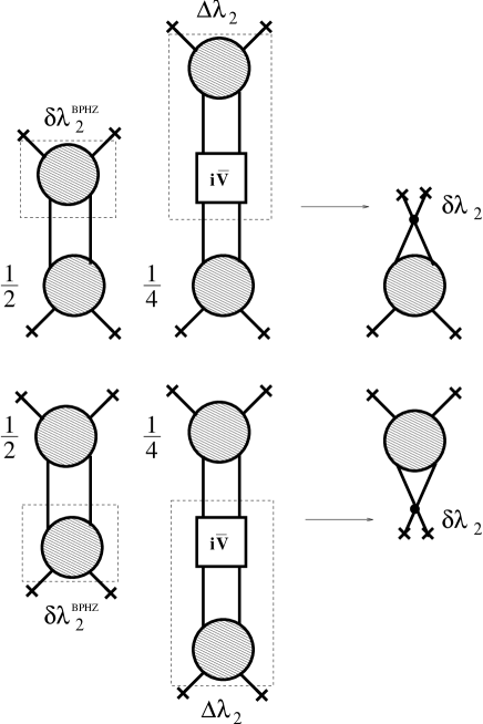
Figure 21: The sub-divergences in the four-point function are nothing but the divergences in $V_{R}$.

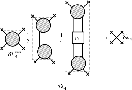
Figure 22: The remaining divergences are only overall divergences. They are thus local and are absorbed in a redefinition of the tree-level contribution to $\delta^{4}\Gamma_{\mbox{\scriptsize int}}^{R}/\delta\phi_{R}^{4}|_{{\bar{G}}_{R}}$. Part of them ($\delta\lambda^{\rm BPHZ}_{4}$) have already been taken into account in the renormalization of the four-point kernel $\delta^{4}\Gamma_{\mbox{\scriptsize int}}/\delta\phi^{4}|_{{\bar{G}}_{R}}$. The rest can be absorbed in a shift $\Delta\lambda_{4}$ of the tree-level contribution to this kernel.

For an algebraic proof, we use Eq. (2.32). As for the functions $\bar{V}_{R}$ and $V_{R}$ above, we use the notations $\Gamma_{R}^{(4)}(p,q,k)\equiv\Gamma_{R}^{(4)}(p,-q,-k,k+q-p)$ and $\Gamma_{R}^{(4)}(p,k)\equiv\Gamma_{R}^{(4)}(p,p,k)$, where $\Gamma_{R}^{(4)}(p_{1},\ldots,p_{4})$ is the four-dimensional Fourier transform of the renormalized four-point function. According to our discussion above Eq. (3.56), we write the kernel

$$\frac{\delta^{4}\Gamma_{\mbox{\scriptsize int}}^{R}}{\delta\phi_{R}^{4}}\Big{|}_{{\bar{G}}_{R}}=\Gamma_{\mbox{\scriptsize int}}^{(4)}({\bar{G}}_{R})=\gamma_{\mbox{\scriptsize int}}^{(4)}({\bar{G}}_{R})-\Delta\lambda_{4}\,,$$ (4.96)

where the function $\gamma_{\mbox{\scriptsize int}}^{(4)}({\bar{G}}_{R})$ has been made finite by means of the BPHZ analysis applied to resummed 2PI diagrams, as described previously. The three channels of Eq. (2.32) contribute the same for what concerns UV-divergences so one can write:

$$\Gamma_{R}^{(4)}(p,k) = \gamma_{\mbox{\scriptsize int}}^{(4)}(p,k)-\Delta\lambda_{4}+\frac{3}{2}\,\int_{q}V_{R}(p,q)\,{\bar{G}}_{R}^{2}(q)\,\Big{(}\Lambda^{\dagger}_{R}(q,k)-\Delta\lambda_{2}\Big{)}$$ (4.97)

$$+$$ finite

$$= \gamma_{\mbox{\scriptsize int}}^{(4)}(p,k)-\Delta\lambda_{4}+\frac{3}{2}\,\int_{q}\Big{(}\Lambda_{R}(p,q)-\Delta\lambda_{2}\Big{)}\,{\bar{G}}_{R}^{2}(q)\,V^{\dagger}_{R}(q,k)$$

$$+ \mbox{finite}\,,$$

where we used the fact that $\Gamma_{R}^{(4)}(p,k)=\Gamma_{R}^{(4)}(k,p)$ – and similarly for $\gamma_{\mbox{\scriptsize int}}^{(4)}(p,k)$ – to write the second line, and where $\Lambda_{R}^{\dagger}(q,k)=\Lambda_{R}(k,q)$ and $V_{R}^{\dagger}(q,k)=V_{R}(k,q)$. The two equations above imply that:

$$\int_{q}V_{R}(p,q)\,{\bar{G}}_{R}^{2}(q)\,\Big{(}\Lambda_{R}^{\dagger}(q,k)-\Delta\lambda_{2}\Big{)} = \int_{q}\Big{(}\Lambda_{R}(p,q)-\Delta\lambda_{2}\Big{)}\,{\bar{G}}_{R}^{2}(q)\,V^{\dagger}_{R}(q,k)$$ (4.98)

$$+ \mbox{finite}\,.$$

From this, and using similar manipulations as for the discussions of the functions $\bar{V}_{R}$ and $V_{R}$, one obtains the following finite equation:

$$\Gamma_{R}^{(4)}(p,k)-\Gamma_{R}^{(4)}(\tilde{p},\tilde{p}) = \gamma_{\mbox{\scriptsize int}}^{(4)}(p,k)-\gamma_{\mbox{\scriptsize int}}^{(4)}(\tilde{p},\tilde{p})$$ (4.99)

$$+\frac{3}{2}\,\int_{q}V_{R}(p,q)\,{\bar{G}}_{R}^{2}(q)\,\Big{\{}\Lambda^{\dagger}_{R}(q,k)-\Lambda^{\dagger}_{R}(q,\tilde{p})\Big{\}}$$

$$+\frac{3}{2}\,\int_{q}\Big{\{}\Lambda_{R}(p,q)-\Lambda_{R}(\tilde{p},q)\Big{\}}\,{\bar{G}}_{R}^{2}(q)\,V^{\dagger}_{R}(q,\tilde{p})$$

$$+\mbox{finite}\,.$$

The contribution $\Delta\lambda_{4}$ to the counterterm $\delta\lambda_{4}$ has been traded for the finite number $\Gamma_{R}^{(4)}(\tilde{p},\tilde{p})=-\lambda_{R}$. Using similar arguments as before, see Eq. (4.1.1), it can be shown that the function $\Gamma_{R}^{(4)}(p,q,k)$ does not contain new divergences.

4.2.3 Higher $n$-point functions

We now show that higher $n$-point functions are automatically finite once the two- and four-point functions have been renormalized. To this aim, we discuss the case of the six-point function in detail. The argument generalizes to arbitrary $n$-point functions. The various topologies appearing in the diagrammatic representation of the six-point function are shown in Fig. 23.

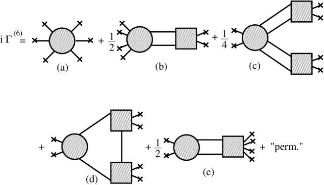
Figure 23: Topologies entering the six-point function. The combinatorial factors are shown. It is understood that each topology comes with the relevant permutations of external legs needed by symmetry.

There, we show the combinatorial factors associated to each topology, arising from the various functional derivatives with the rules described earlier in Sec. 2.2. We do not specify explicitly the various possible orderings of the external legs as this plays no role for the present argument. It is understood that each topology comes with all the permutations of its external legs needed to symmetrize it in a proper way, that is according to the symmetry property of the six-point function. Most of the diagrams in Fig. 23 are explicitly finite. Diagram (a) is a six-point 2PI kernel, namely $\delta^{6}\Gamma_{\mbox{\scriptsize int}}^{R}/\delta\phi_{R}^{6}|_{{\bar{G}}_{R}}=\Gamma_{\mbox{\scriptsize int}}^{(6)}({\bar{G}}_{R})$, and is thus renormalized by the 2PI BPHZ procedure described previously. Diagrams (b) and (c) both contain loop integrals involving the six-point kernels $\delta^{6}\Gamma_{\mbox{\scriptsize int}}^{R}/\delta\phi_{R}^{4}\delta G_{R}|_{{\bar{G}}_{R}}=\delta\Gamma_{\mbox{\scriptsize int}}^{(4)}/\delta G_{R}|_{{\bar{G}}_{R}}$ and $\delta^{6}\Gamma_{\rm int}^{R}/\delta\phi_{R}^{2}\delta G_{R}^{2}|_{{\bar{G}}_{R}}=\delta^{2}\Gamma_{\rm int}^{(2)}/\delta G_{R}^{2}|_{{\bar{G}}_{R}}$, the propagator ${\bar{G}}_{R}$ and the box with two external legs $\delta^{2}\bar{\Sigma}_{R}/\delta\phi_{R}^{2}\equiv iV_{R}$. Each of these objects is finite. Thus potential divergences in diagrams (b) and (c) can only arise from the loop integrals. By power counting there is no overall divergence thus one has to look for potential sub-divergences. The only possible candidates are depicted in Fig. 24 in the case of diagram (b).

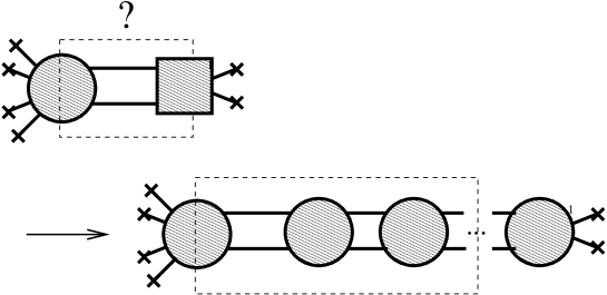
Figure 24: The only possible origin for a four-point sub-divergence in the contribution (b) to the six-point function, see Fig. 23.

Clearly, the square box being a 1PI structure, one needs to cut at least two lines of it in order to draw a four-point box – corresponding to a coupling sub-divergence. This implies that one needs to cut not more than two lines in the six-point kernel involved in this diagram. This is, however, not possible due to the 2PI character of the latter (cf. Appendix LABEL:2PItop). We conclude that there are no sub-divergences in diagram (b), which is thus finite. The same argument applies to diagram (c) as well. Diagrams (d) and (e) are more subtle since they contain the four-point kernel $\Lambda_{R}-\Delta\Lambda_{2}$, which is not finite. If one would replace this kernel by its finite part $\Lambda_{R}$, diagram (d) would be finite by the same argument as the one used above for diagrams (b) and (c). However, there is an extra contribution arising from $\Delta\lambda_{2}$, which is infinite. In fact, as we now show, this contribution is crucial to remove divergences which are present in diagram (e). To see this explicitly, we first have to discuss the renormalization of the function $\delta^{4}\bar{\Sigma}_{R}/\delta\phi_{R}^{4}$, involved in diagram (e).

As discussed earlier in Sec. 2.2, this function satisfies a linear integral equation. In Fig. 25, we show the relevant topologies appearing in this equation together with the appropriate combinatorial factors. As before, it is understood that each topology comes with the relevant permutations of external legs needed to ensure the correct symmetry properties according to the LHS.

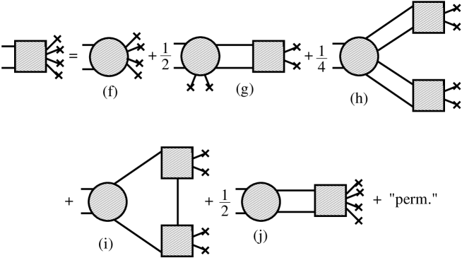
Figure 25: Topologies appearing in the self-consistent equation for $\delta^{4}\bar{\Sigma}_{R}/\delta\phi_{R}^{4}$. The combinatorial factors are shown. It is understood that each topology comes with the relevant permutations of external legs needed by symmetry.

Using the same argument as for the diagram (a)-(c) in Fig. 23, we conclude that the contributions (f)-(h) are finite, whereas diagrams (i) and (j) are infinite. Diagram (j) involves the unknown function $\delta^{4}\bar{\Sigma}_{R}/\delta\phi_{R}^{4}$ itself. To pursue the discussion, it is thus more appropriate to solve for $\delta^{4}\bar{\Sigma}_{R}/\delta\phi_{R}^{4}$ using the vertex function $\bar{V}_{R}$, as explained in Sec. 2.2. The topologies appearing in the solution are depicted in Fig. 26 with the relevant combinatorial factors.

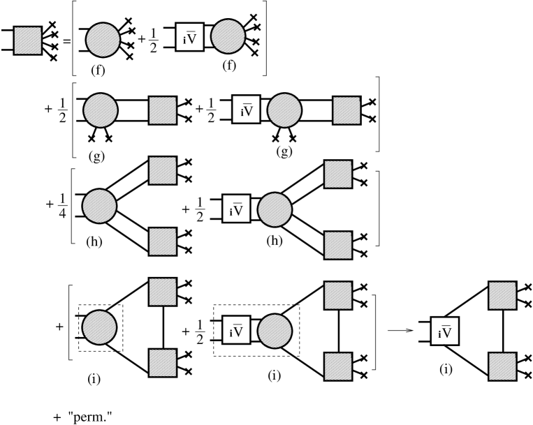
Figure 26: Solution and finiteness of $\delta^{4}\bar{\Sigma}_{R}/\delta\phi_{R}^{4}$: The only two potential divergent diagrams combine to a finite term (last line).

As expressed in Eq. (2.21), one obtains all the previous diagrams of Fig. 25 but (j), plus the same diagrams convoluted with the function $\bar{V}_{R}$. Using a similar reasoning as above, exploiting the 2PI character of the kernels, one finds that all the diagrams appearing in the first three lines of Fig. 26 – that is those containing diagrams (f)-(h) as a sub-diagram – are explicitly finite. The only divergent contributions are those containing diagrams (i), shown on the last line of the figure. These two divergent diagrams combine to a finite term by means of Eq. (2.29), as represented in Fig. 26. This shows that the function $\delta^{4}\bar{\Sigma}_{R}/\delta\phi_{R}^{4}$ is finite.

We now return to the six-point function. We insert the diagrams of Fig. 26 into diagram (e) of Fig. 23. This generates structures such as the one depicted in Fig. 27, which shows the convolution of diagram (e) with the first line of Fig. 26, that is with the diagrams containing (f) as a sub-structure.

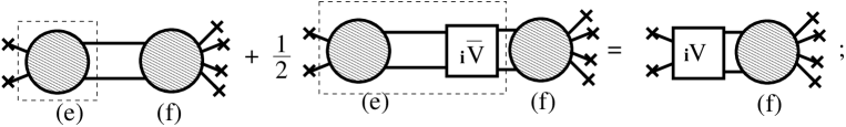
Figure 27: Structures appearing in the six-point function after inserting the expression for $\delta^{4}\bar{\Sigma}_{R}/\delta\phi_{R}^{4}$ represented on Fig. 26 into the diagram (e) of Fig. 23. Each contribution on the LHS is potentially divergent, but their sum is finite.

Each separate contribution containing the sub-diagram (f) contains potential sub-divergences. However, using Eq. (2.30) one sees that their sum combines in a simpler structure involving the finite function $V_{R}$, as shown in Fig. 27. Exploiting the 2PI character of the kernel $\delta\Gamma_{\mbox{\scriptsize int}}^{(4)}/\delta G_{R}|_{{\bar{G}}_{R}}$ – which corresponds to the diagram (f) – one concludes that the resulting structure is finite. A similar reasoning shows that the insertion of the second and the third lines of Fig. 26, i.e. those involving the sub-diagrams (g) and (h) respectively, into diagram (e) of Fig. 23 also leads to finite structures involving the function $V_{R}$. In contrast, insertion of the last diagram of Fig. 26 – involving the sub-diagram (i) – into (e) is not enough to generate a finite structure. However, the resulting contribution combines with diagram (d) of Fig. 23 into a structure involving the finite function $V_{R}$, as shown in Fig. 28.

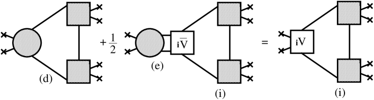
Figure 28: Contributions to the six-point function. The structure involving sub-diagram (i) arises after plugging the expression of $\delta^{4}\bar{\Sigma}_{R}/\delta\phi_{R}^{4}$ represented on Fig. 26 into the diagram (e) of Fig. 23. The latter combines with the previous contribution (d) into a finite structure by means of Eq. (2.30).

The latter contribution is finite by similar arguments as before. Thus we conclude that the six-point function is finite, as announced.

The present analysis straightforwardly generalizes to the case of higher $n$-point functions. Although the number of terms to consider increases rapidly, the relevant structures needed for the cancellation of divergences by means of Eqs. (2.29) and (2.30) always appear. In particular, using a similar reasoning as above, one can show by recurrence that all the functions $\delta^{2n}\bar{\Sigma}_{R}/\delta\phi_{R}^{2n}$ as well as all $n$-point functions $\Gamma_{R}^{2n}$ are finite. Finally, we mention that the zero-point function, namely $\Gamma_{\mbox{\scriptsize int}}^{(0)}[{\bar{G}}_{R}]$, can be shown to be finite up to an irrelevant, field and temperature independent infinite constant [16].

5 Renormalization at non-vanishing field

It has been shown above that the resummed effective action is finite. For this we have employed derivatives of the effective action taken at $\phi_{R}=0$. As far as UV singularities are concerned, it thus follows that derivatives at $\phi_{R}\neq 0$ are also finite. The latter are exactly the $n$-point functions that one has to consider in the broken phase. It is therefore sufficient to renormalize the resummed effective action in the symmetric phase. Divergences are simply reshuffled among the various $n$-point functions as compared to the zero-field case.

In this section, we illustrate these general arguments for a number of relevant examples. We first discuss the divergences appearing in the equation for ${\bar{G}}_{R}(\phi_{R})$ for arbitrary $\phi_{R}\neq 0$. We show that to make the latter finite, one does not only need the counterterms determined from the renormalization of ${\bar{G}}_{R}(\phi_{R}=0)$, but also the counterterms used to renormalize the two-point function $\Gamma^{(2)}_{R}(\phi_{R}=0)$. We also discuss the UV singularities of the two-point function $\Gamma_{R}^{(2)}(\phi_{R})$. The renormalization of the latter for arbitrary $\phi_{R}\neq 0$ is connected to the renormalization of all higher $n$-point functions in the symmetric phase.

5.1 Renormalization of ${\bar{G}}_{R}(\phi_{R})$

A diagrammatic analysis reveals that the divergences appearing in the function ${\bar{G}}_{R}(\phi_{R})$ for non-zero field are precisely those of the functions ${\bar{G}}_{R}(\phi_{R}=0)$ and part of those in $\Gamma^{(2)}_{R}(\phi_{R}=0)$. The renormalization of ${\bar{G}}_{R}(\phi_{R})$, therefore, does not only involve the counterterms $\delta Z_{0}$, $\delta m^{2}_{0}$, $\delta\lambda_{0}$, etc., needed to renormalize the former, but also the coupling counterterm $\delta\lambda_{2}$, determined from the renormalization of the latter. Here, we present an algebraic discussion of these aspects. Using the field-expansion (3.47), the self-energy $\bar{\Sigma}_{R}(\phi_{R})$ may be written as

$$\bar{\Sigma}_{R}(\phi_{R})=2i\left\{\frac{\delta\Gamma_{\mbox{\scriptsize int}}^{(0)}}{\delta G_{R}}\Big{|}_{{\bar{G}}_{R}}+\frac{1}{2}\phi_{R}^{2}\frac{\delta\Gamma_{\mbox{\scriptsize int}}^{(2)}}{\delta G_{R}}\Big{|}_{{\bar{G}}_{R}}+\sum_{n\geq 2}\frac{1}{(2n)!}\phi_{R}^{2n}\frac{\delta\Gamma_{\mbox{\scriptsize int}}^{(2n)}}{\delta G_{R}}\Big{|}_{{\bar{G}}_{R}}\right\}\,.$$ (5.100)

where ${\bar{G}}_{R}\equiv{\bar{G}}_{R}(\phi_{R})$. Applying the same technique as in the previous section, and generalizing the notations of Secs. 4.1.2 and 4.1.4 to the case with non-vanishing field, we obtain

$$\bar{\Sigma}_{0}(p) = -i\delta m_{0}^{2}+\frac{1}{2}\,\int_{q}\Big{(}\bar{\Lambda}_{2}(p,q)-\Delta\lambda_{0}\Big{)}\,\delta{\bar{G}}(q)$$ (5.101)

$$+\frac{i}{2}\,\phi_{R}^{2}\Big{(}\Lambda_{2}(0,p)-\Delta\lambda_{2}\Big{)}+\bar{\Sigma}_{r}(p)\,,$$

where the function $\delta{\bar{G}}(p)$ can be written as in Eq. (4.77). The above equation can be rewritten as ($\tilde{p}$ being the renormalization point):

$$\bar{\Sigma}_{0}(p) = -i\delta m_{0}^{2}+\frac{1}{2}\,\int_{q}\Big{(}\bar{\Lambda}_{2}(\tilde{p},q)-\Delta\lambda_{0}\Big{)}\,\delta{\bar{G}}(q)$$ (5.102)

$$+\frac{i}{2}\,\phi_{R}^{2}\Big{(}\Lambda_{2}(0,p)-\Delta\lambda_{2}\Big{)}+\bar{\Sigma}^{\prime}_{r}(p)\,,$$

where the functions $\bar{\Sigma}_{r}(p)$ and $\bar{\Sigma}^{\prime}_{r}(p)$ are finite and $\sim 1/p$ at large $p$. They are related to each other as in Eq. (4.81). Here, we have used the fact that possible subdivergences in the terms higher than quadratic in the field in Eq. (5.100) have been removed by means of the previously described BPHZ analysis. Moreover, these contributions decrease at least as $\sim 1/p$ at large $p$, which follows from power counting arguments and the 2PI character of the kernels $\delta\Gamma_{\mbox{\scriptsize int}}^{(2n)}/\delta G_{R}|_{{\bar{G}}_{R}}$. Using the vertex equation for $\bar{V}_{R}\equiv\bar{V}_{R}(\phi_{R})$, with propagators replaced by ${\bar{G}}_{2}$, we get:

$$\bar{\Sigma}_{0}(p) = -i\delta m_{0}^{2}+\bar{\Sigma}^{\prime}_{r}(p)+\frac{i}{2}\,\phi_{R}^{2}\Big{(}\Lambda_{2}(0,p)-\Delta\lambda_{2}\Big{)}+\frac{1}{2}\,\int_{q}\,\bar{V}_{2}(\tilde{p},q)\,\delta{\bar{G}}(q)$$ (5.103)

$$-\frac{1}{4}\,\int_{q}\int_{k}\,\bar{V}_{2}(\tilde{p},q)\,{\bar{G}}_{2}^{2}(q)\,\Big{(}\bar{\Lambda}_{2}(q,k)-\Delta\lambda_{0}\Big{)}\,\delta{\bar{G}}(k)\,.$$

In the third term, the integral over $k$ is known from Eq. (5.101):

$$\bar{\Sigma}_{0}(p) = -i\delta m_{0}^{2}+\bar{\Sigma}^{\prime}_{r}(p)+\frac{1}{2}\,\int_{q}\,\bar{V}_{2}(\tilde{p},q)\,\delta{\bar{G}}(q)$$

$$- \frac{1}{2}\,\int_{q}\,\bar{V}_{2}(\tilde{p},q)\,{\bar{G}}_{2}^{2}(q)\,\Big{\{}\bar{\Sigma}_{0}(q)-\bar{\Sigma}_{r}(q)+i\delta m_{0}^{2}\Big{\}}$$

$$+ \frac{i}{2}\phi_{R}^{2}\Big{\{}\Lambda_{2}(0,p)-\Delta\lambda_{2}+\frac{1}{2}\int_{q}\bar{V}_{2}(\tilde{p},q)\,{\bar{G}}_{2}^{2}(q)\,\Big{(}\Lambda_{2}(0,q)-\Delta\lambda_{2}\Big{)}\Big{\}}.$$

Using the expression of the function $\delta{\bar{G}}(p)$ (cf. Eq. (4.77)), one observes that potentially divergent terms depending on $\bar{\Sigma}_{0}$ vanish and we are left with

$$\bar{\Sigma}_{0}(p) = \frac{1}{2}\,\int_{q}\,\bar{V}_{2}(\tilde{p},q)\,\Big{\{}{\bar{G}}_{r}(q)+{\bar{G}}_{2}^{2}(q)\,\bar{\Sigma}_{r}(q)\Big{\}}+\bar{\Sigma}^{\prime}_{r}(p)$$ (5.105)

$$-i\delta m_{0}^{2}-\frac{i}{2}(m_{R}^{2}+\delta m^{2}_{0})\,\int_{q}\,\bar{V}_{2}(\tilde{p},q)\,{\bar{G}}_{2}^{2}(q)$$

$$+\frac{i}{2}\,\phi_{R}^{2}\Big{\{}\Lambda_{2}(0,p)-\Lambda_{2}(0,\tilde{p})+V_{2}(0,\tilde{p})\Big{\}}\,,$$

where we have used the defining equation for the finite number $V_{2}(0,\tilde{p})$ (cf. Eq. (4.86)) to absorb the counterterm $\Delta\lambda_{2}$. The above equation has the same structure as the corresponding Eq. (4.84) for the case of a vanishing field, except for the last line, which is finite due to the counterterm $\delta\lambda_{2}$.

5.2 The two-point function

For the purpose of discussing the structure of UV divergences due to the presence of a non-vanishing field, it is sufficient to assume the following field-expansion of the two-point function:

$$\Gamma_{R}^{(2)}(\phi_{R})=\Gamma_{R}^{(2)}(0)+\frac{1}{2}\phi_{R}^{2}\Gamma_{R}^{(4)}(0)+\frac{1}{4!}\phi_{R}^{4}\Gamma_{R}^{(6)}(0)+\ldots\,.$$ (5.106)

The latter is finite for arbitrary field, provided the theory has been properly renormalized at $\phi_{R}=0$, that is all $n$-point functions have been made finite in the symmetric phase. Equation (5.106) also shows how the divergences appearing in the symmetric phase are reshuffled in the presence of a non-vanishing field expectation value. In particular, unlike in the symmetric case, all the counterterms of the theory are needed to renormalize the two-point function.

It is instructive to see how Eq. (5.106) arises from the expression of the two-point function in terms of 2PI kernels. Here, we illustrate this for the example of the term quadratic in the field, which involves the four-point function at $\phi_{R}=0$. In the broken phase, the non-trivial part of the two-point function is no longer simply given by the kernel $\delta^{2}\Gamma_{\mbox{\scriptsize int}}^{R}/\delta\phi_{R}^{2}|_{{\bar{G}}_{R}}$, but receives a new contribution which involves the function $\delta\bar{\Sigma}_{R}/\delta\phi_{R}$, as depicted in Fig. 3 (cf. also Eq. (2.16)). In the present $Z_{2}$-symmetric theory, the latter vanishes in the symmetric phase. In the general case, it satisfies the integral equation (2.17), represented in Fig. 3, expressed in terms of renormalized kernels. The latter has the general form of Eq. (2.18) and can be solved in terms of the finite vertex function $\bar{V}_{R}$, as in Eq. (2.21). Plugging the resulting expression into the expression for the two-point function (cf. Eq. (2.16)) one finds

$$\Gamma^{(2)}_{R}(\phi_{R}) = iG_{0R}^{-1}+\frac{\delta^{2}\Gamma_{\mbox{\scriptsize int}}^{R}}{\delta\phi_{R}^{2}}\Big{|}_{{\bar{G}}_{R}}+2i\frac{\delta^{2}\Gamma_{\mbox{\scriptsize int}}^{R}}{\delta\phi_{R}\delta G_{R}}\Big{|}_{{\bar{G}}_{R}}{\bar{G}}_{R}^{2}\frac{\delta^{2}\Gamma_{\mbox{\scriptsize int}}^{R}}{\delta G_{R}\delta\phi_{R}}\Big{|}_{{\bar{G}}_{R}}$$ (5.107)

$$-\frac{\delta^{2}\Gamma_{\mbox{\scriptsize int}}^{R}}{\delta\phi_{R}\delta G_{R}}\Big{|}_{{\bar{G}}_{R}}{\bar{G}}_{R}^{2}\bar{V}_{R}{\bar{G}}_{R}^{2}\frac{\delta^{2}\Gamma_{\mbox{\scriptsize int}}^{R}}{\delta G_{R}\delta\phi_{R}}\Big{|}_{{\bar{G}}_{R}}\,,$$

where ${\bar{G}}_{R}\equiv{\bar{G}}_{R}(\phi_{R})$ and $\bar{V}_{R}\equiv\bar{V}_{R}(\phi_{R})$. Equation (5.107) is depicted in Fig. 29. Using again power counting and the 2PI character of the kernels, one finds that possible sub-divergences in the last two terms of Eq. (5.107) can only arise from the quadratic field-dependence of the

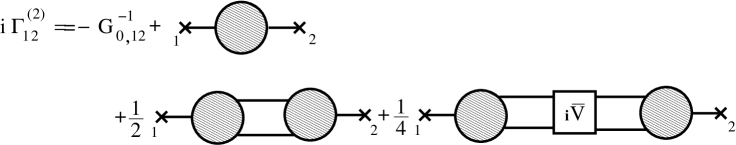
Figure 29: The two-point function in the broken phase $\Gamma^{(2)}_{R}(\phi_{R})$, in terms of the vertex function $\bar{V}_{R}$.

latter. Using the field-expansion

$$\frac{\delta^{2}\Gamma_{\mbox{\scriptsize int}}^{R}}{\delta\phi\delta G_{R}}\Big{|}_{{\bar{G}}_{R}}=\phi_{R}\frac{\delta\Gamma_{\mbox{\scriptsize int}}^{(2)}}{\delta G_{R}}\Big{|}_{{\bar{G}}_{R}}+\frac{1}{3!}\phi_{R}^{3}\frac{\delta\Gamma_{\mbox{\scriptsize int}}^{(4)}}{\delta G_{R}}\Big{|}_{{\bar{G}}_{R}}+\dots\,,$$ (5.108)

one finds that the quadratic field-dependence of the last two terms of Eq. (5.107) is given by

$$2i\phi_{R}\,\frac{\delta\Gamma_{\mbox{\scriptsize int}}^{(2)}}{\delta G_{R}}\Big{|}_{{\bar{G}}_{R}(0)}\Big{\{}{\bar{G}}_{R}^{2}(0)+\frac{i}{2}{\bar{G}}_{R}^{2}(0)\,\bar{V}_{R}(0)\,{\bar{G}}_{R}^{2}(0)\Big{\}}\frac{\delta\Gamma_{\mbox{\scriptsize int}}^{(2)}}{\delta G_{R}}\Big{|}_{{\bar{G}}_{R}(0)}\phi_{R}$$

$$=i\phi_{R}\,V_{R}(0)\,{\bar{G}}_{R}^{2}(0)\,\frac{\delta\Gamma_{\mbox{\scriptsize int}}^{(2)}}{\delta G_{R}}\Big{|}_{{\bar{G}}_{R}(0)}\phi_{R}\,,$$ (5.109)

where we used Eqs. (2.27) and (2.30) to write the result in a compact form involving the function $V_{R}(\phi_{R}=0)$. We see that the divergences contained in this contribution have a similar structure as that of the four-point function in the symmetric phase (cf. Eqs. (2.32) and (2.3)).

All the remaining divergences in the two-point function at non-vanishing field in fact come from the second term on the RHS of Eq. (5.107), which was already present in the symmetric phase. The explicit field dependence of the latter is given by

$$\frac{\delta^{2}\Gamma_{\mbox{\scriptsize int}}^{R}}{\delta\phi_{R}^{2}}\Big{|}_{{\bar{G}}_{R}}=\Gamma_{\mbox{\scriptsize int}}^{(2)}({\bar{G}}_{R})+\frac{1}{2}\phi_{R}^{2}\Gamma_{\mbox{\scriptsize int}}^{(4)}({\bar{G}}_{R})+\dots\,.$$ (5.110)

One observes that the explicit quadratic term, involving $\Gamma_{\mbox{\scriptsize int}}^{(4)}[{\bar{G}}_{R}]$, almost combines with the quadratic term (5.109) to give the four-point function, as in Eq. (2.32). However, one of the three possible channels appearing in this equation is missing. In fact, the latter arise from the implicit field-dependence of the kernels, that is through the field-dependence of ${\bar{G}}_{R}(\phi_{R})$. Indeed, writing

$${\bar{G}}_{R}(\phi_{R})={\bar{G}}_{R}(0)+\frac{i}{2}\phi_{R}^{2}\,V_{R}(0)\,{\bar{G}}_{R}^{2}(0)+\ldots\,,$$ (5.111)

where we used the definition of the vertex function $V_{R}(0)$, cf. Eq. (2.28), one obtains:

$$\Gamma_{\mbox{\scriptsize int}}^{(2)}({\bar{G}}_{R})=\Gamma_{\mbox{\scriptsize int}}^{(2)}({\bar{G}}_{R}(0))+\frac{i}{2}\phi_{R}^{2}\,V_{R}(0)\,{\bar{G}}_{R}^{2}(0)\,\frac{\delta\Gamma_{\mbox{\scriptsize int}}^{(2)}}{\delta G_{R}}\Big{|}_{{\bar{G}}_{R}(0)}+\ldots\,.$$ (5.112)

When inserted into the expression (5.107) for the two-point function, the first term on the RHS of Eq. (5.112) gives the first term in the field-expansion (5.106), that is simply the two-point function in the symmetric phase. The term quadratic in the field in Eq. (5.112) gives the missing channel needed to reconstruct the four-point function at vanishing field, as mentioned above. Indeed, collecting all terms quadratic in the field in Eqs. (5.109), (5.110) and (5.112) and using the fact that $\delta\Gamma_{\mbox{\scriptsize int}}^{(2)}/\delta G_{R}|_{{\bar{G}}_{R}(0)}=(\Lambda_{R}(0)-\Delta\lambda_{2})/2$, one finds that the quadratic field-dependence of the two-point function (5.107) is given by (see Eq. (2.32)):

$$\frac{1}{2}\phi_{R}^{2}\Big{\{}\Gamma_{\mbox{\scriptsize int}}^{(4)}({\bar{G}}_{R}(0))+\frac{3i}{2}(\Lambda_{R}(0)-\Delta\lambda_{2})\,{\bar{G}}_{R}^{2}(0)\,V_{R}(0)\Big{\}}=\frac{1}{2}\phi_{R}^{2}\Gamma_{R}^{(4)}(0)\,,$$ (5.113)

as expected. Higher order terms in the field-expansion (5.106) can be obtained along similar lines.

6 Multiple scalar fields

So far, we have been concerned with the case of a single scalar field theory. In this section, we show how the previous results generalize to theories with multiple fields. In particular, this will demonstrate that all the results established in the previous sections hold, provided all counterterms allowed by the symmetries of the theory are included.

6.1 Symmetries

As an example, we consider the case of an $O(N)$-symmetric theory. The 2PI functional is symmetric under simultaneous rotations of the field $\phi_{R}^{a}(x)$ and of the propagator $G_{R}^{ab}(x,y)$:

$$\phi_{R}^{a}(x) \to {\mathcal{R}}^{ab}\phi_{R}^{b}(x)$$ (6.114)

$$G_{R}^{ab}(x,y) \to {\mathcal{R}}^{ac}{\mathcal{R}}^{bd}G_{R}^{cd}(x,y)$$ (6.115)

where ${\mathcal{R}}$ denotes an arbitrary $O(N)$ rotation. The generalization of Eq. (3.56) to the $O(N)$ case, therefore, has the general structure:

$$\Gamma_{\mbox{\scriptsize int}}^{R}[\phi_{R},G_{R}] = \gamma_{\mbox{\scriptsize int}}[\phi_{R},G_{R}]$$

$$- \int_{x}\,\Big{\{}\frac{\Delta\lambda^{(\mbox{\scriptsize A})}_{0}}{4!N}\,G_{R}^{aa}(x,x)\,G_{R}^{bb}(x,x)+\frac{\Delta\lambda^{(\mbox{\scriptsize B})}_{0}}{12N}\,G_{R}^{ab}(x,x)\,G_{R}^{ab}(x,x)$$

$$+ \frac{\Delta\lambda^{(\mbox{\scriptsize A})}_{2}}{12N}\,G_{R}^{aa}(x,x)\phi_{R}^{b}(x)\phi_{R}^{b}(x)+\frac{\Delta\lambda^{(\mbox{\scriptsize B})}_{2}}{6N}\,G_{R}^{ab}(x,x)\phi_{R}^{a}(x)\phi_{R}^{b}(x)$$

$$+ \frac{\Delta\lambda_{4}}{4!N}\,\phi_{R}^{a}(x)\phi_{R}^{a}(x)\phi_{R}^{b}(x)\phi_{R}^{b}(x)\Big{\}}\,.$$

Extracting the mass and field counterterms as in Eq. (3.57), we write:

$$\gamma_{\mbox{\scriptsize int}}[\phi_{R},G_{R}] = \tilde{\gamma}_{\mbox{\scriptsize int}}[\phi_{R},G_{R}]-\frac{1}{2}\int_{x}\,\Big{\{}\phi_{R}^{a}(x)\left[\delta Z_{0}\square_{x}+\delta m^{2}_{0}\right]\phi_{R}^{a}(x)$$ (6.117)

$$+\left[\delta Z_{2}\square_{x}+\delta m^{2}_{2}\right]G_{R}^{aa}(x,y)|_{y=x}\Big{\}}\,.$$

The pairs of counterterms $\Delta\lambda^{(\mbox{\scriptsize A})}_{0}$ and $\Delta\lambda^{(\mbox{\scriptsize A})}_{2}$ as well as $\Delta\lambda^{(\mbox{\scriptsize B})}_{0}$ and $\Delta\lambda^{(\mbox{\scriptsize B})}_{2}$ are independent of each other and may have different expressions for a given approximation. As for the single scalar field, their values are determined by imposing renormalization conditions on the various components of the renormalized functions $\bar{V}_{R}$ and $V_{R}$. The latter satisfy trivial generalizations of the integral equations (2.29) and (2.30), respectively, where the subscript $1,2,\dots$ now denote space-time variables as well as internal $O(N)$ indices.

As an illustration, we consider the renormalization of $\bar{V}_{R}$ at $\phi_{R}^{a}=0$. Exploiting the symmetries of the functions $\bar{\Lambda}_{R}\equiv\bar{\Lambda}_{R}^{ab;cd}(x,y;z,t)$ and $\bar{V}_{R}\equiv\bar{V}_{R}^{ab;cd}(x,y;z,t)$, we write

$$\bar{\Lambda}_{R}^{ab;cd}(x,y;z,t) = \delta^{ab}\delta^{cd}\,\bar{\Lambda}^{(\mbox{\scriptsize A})}_{R}(x,y;z,t)$$ (6.118)

$$+ \delta^{ac}\delta^{bd}\,\bar{\Lambda}^{(\mbox{\scriptsize B})}_{R}(x,y;z,t)+\delta^{ad}\delta^{bc}\,\bar{\Lambda}^{(\mbox{\scriptsize B})}_{R}(x,y;t,z)\,,$$

with $\bar{\Lambda}^{(\mbox{\scriptsize A})}_{R}(x,y;z,t)=\bar{\Lambda}^{(\mbox{\scriptsize A})}_{R}(y,x;z,t)=\bar{\Lambda}^{(\mbox{\scriptsize A})}_{R}(x,y;t,z)$ and $\bar{\Lambda}^{(\mbox{\scriptsize B})}_{R}(x,y;z,t)=\bar{\Lambda}^{(\mbox{\scriptsize B})}_{R}(y,x;t,z)$, and similarly for $\bar{V}_{R}^{ab;cd}(x,y;z,t)$. One also has

$${\bar{G}}_{R}^{ab}(x,y)=\delta^{ab}\,{\bar{G}}_{R}(x,y)\,,$$ (6.119)

with ${\bar{G}}_{R}(x,y)={\bar{G}}_{R}(y,x)$. Using Eqs. (6.118) and (6.119), one obtains the integral equations satisfied by the various components $\bar{V}^{(\mbox{\scriptsize A})}_{R}$ and $\bar{V}^{(\mbox{\scriptsize B})}_{R}$ from the generalization of Eq. (2.29) to the $O(N)$ case. For notational convenience, we write the latter in terms of bare quantities

$$\bar{V}^{(\mbox{\scriptsize A})} = \bar{\Lambda}^{(\mbox{\scriptsize A})}+\frac{iN}{2}\bar{V}^{(\mbox{\scriptsize A})}{\bar{G}}^{2}\bar{\Lambda}^{(\mbox{\scriptsize A})}+i\bar{V}^{(\mbox{\scriptsize A})}{\bar{G}}^{2}\bar{\Lambda}^{(\mbox{\scriptsize B})}+i\bar{V}^{(\mbox{\scriptsize B})}{\bar{G}}^{2}\bar{\Lambda}^{(\mbox{\scriptsize A})}$$ (6.120)

$$= \bar{\Lambda}^{(\mbox{\scriptsize A})}+\frac{iN}{2}\bar{\Lambda}^{(\mbox{\scriptsize A})}{\bar{G}}^{2}\bar{V}^{(\mbox{\scriptsize A})}+i\bar{\Lambda}^{(\mbox{\scriptsize B})}{\bar{G}}^{2}\bar{V}^{(\mbox{\scriptsize A})}+i\bar{\Lambda}^{(\mbox{\scriptsize A})}{\bar{G}}^{2}\bar{V}^{(\mbox{\scriptsize B})}\,,$$

and

$$\bar{V}^{(\mbox{\scriptsize B})}=\bar{\Lambda}^{(\mbox{\scriptsize B})}+i\bar{V}^{(\mbox{\scriptsize B})}{\bar{G}}^{2}\bar{\Lambda}^{(\mbox{\scriptsize B})}=\bar{\Lambda}^{(\mbox{\scriptsize B})}+i\bar{\Lambda}^{(\mbox{\scriptsize B})}{\bar{G}}^{2}\bar{V}^{(\mbox{\scriptsize B})}\,.$$ (6.121)

The corresponding equations for renormalized quantities are obtained using the relations $G=ZG_{R}$ as well as $Z^{2}\bar{\Lambda}^{(\mbox{\scriptsize A})}=\bar{\Lambda}^{(\mbox{\scriptsize A})}_{R}-\Delta\lambda^{(\mbox{\scriptsize A})}_{0}$ and $Z^{2}\bar{V}^{(\mbox{\scriptsize A})}=\bar{V}^{(\mbox{\scriptsize A})}_{R}$, and similarly for $\bar{\Lambda}^{(\mbox{\scriptsize B})}$ and $\bar{V}^{(\mbox{\scriptsize B})}$. Equation (6.121) has the same structure as Eq. (2.29) for the case $N=1$ discussed in this paper. It can, therefore, be made finite by the single shift $\Delta\lambda^{(\mbox{\scriptsize B})}_{0}$. Equation (6.120) mixes the various kernels $\bar{\Lambda}^{(\mbox{\scriptsize A})}_{R}$ and $\bar{\Lambda}^{(\mbox{\scriptsize B})}_{R}$ and the associated counterterms $\Delta\lambda^{(\mbox{\scriptsize A})}_{0}$ and $\Delta\lambda^{(\mbox{\scriptsize B})}_{0}$. Iterating this integral equation in powers of the kernels $\bar{\Lambda}^{(\mbox{\scriptsize A})}_{R}$ and $\bar{\Lambda}^{(\mbox{\scriptsize B})}_{R}$ and exploiting, as before, the two-particle-irreducibility of the latter, one finds that, once $\Delta\lambda^{(\mbox{\scriptsize B})}_{0}$ has been adjusted to renormalize $\bar{V}^{(\mbox{\scriptsize B})}_{R}$, all the remaining divergences can be absorbed in the shift $\Delta\lambda^{(\mbox{\scriptsize A})}_{0}$. Alternatively, employing the same steps as for the case $N=1$ (cf. Eq. (4.1.1)), one obtains the following finite equation for $\bar{V}^{(\mbox{\scriptsize A})}_{R}(p,k)\equiv\bar{V}^{(\mbox{\scriptsize A})}_{R}(p,-p,-k,k)$ in Euclidean momentum space:

$$\bar{V}^{(\mbox{\scriptsize A})}_{R}(p,k)-\bar{V}^{(\mbox{\scriptsize A})}_{R}(\tilde{p},\tilde{p})=\bar{\Lambda}^{(\mbox{\scriptsize A})}_{R}(p,k)-\bar{\Lambda}^{(\mbox{\scriptsize A})}_{R}(\tilde{p},\tilde{p})$$

$$\quad+\frac{N}{2}\,\int_{q}\,\Big{\{}\bar{V}^{(\mbox{\scriptsize A})}_{R}(p,q)\,{\bar{G}}_{R}^{2}(q)\,\Delta\bar{\Lambda}^{(\mbox{\scriptsize A})}_{R}(k,q)+\Delta\bar{\Lambda}^{(\mbox{\scriptsize A})}_{R}(p,q)\,{\bar{G}}_{R}^{2}(q)\,\bar{V}^{(\mbox{\scriptsize A})}_{R}(\tilde{p},q)\Big{\}}$$

$$\qquad+\int_{q}\,\Big{\{}\bar{V}^{(\mbox{\scriptsize A})}_{R}(p,q)\,{\bar{G}}_{R}^{2}(q)\,\Delta\bar{\Lambda}^{(\mbox{\scriptsize B})}_{R}(k,q)+\Delta\bar{\Lambda}^{(\mbox{\scriptsize A})}_{R}(p,q)\,{\bar{G}}_{R}^{2}(q)\,\bar{V}^{(\mbox{\scriptsize B})}_{R}(\tilde{p},q)\Big{\}}$$

$$\qquad+\int_{q}\,\Big{\{}\bar{V}^{(\mbox{\scriptsize B})}_{R}(p,q)\,{\bar{G}}_{R}^{2}(q)\,\Delta\bar{\Lambda}^{(\mbox{\scriptsize A})}_{R}(k,q)+\Delta\bar{\Lambda}^{(\mbox{\scriptsize B})}_{R}(p,q)\,{\bar{G}}_{R}^{2}(q)\,\bar{V}^{(\mbox{\scriptsize A})}_{R}(\tilde{p},q)\Big{\}},$$

where $\Delta\bar{\Lambda}^{(\mbox{\scriptsize A})}_{R}(p,q)\equiv\bar{\Lambda}^{(\mbox{\scriptsize A})}_{R}(p,q)-\bar{\Lambda}^{(\mbox{\scriptsize A})}_{R}(\tilde{p},q)$ and similarly for $\Delta\bar{\Lambda}^{(\mbox{\scriptsize B})}_{R}(p,q)$. The counterterm $\Delta\lambda^{(\mbox{\scriptsize A})}_{0}$ is replaced by the finite number $\bar{V}^{(\mbox{\scriptsize A})}_{R}(\tilde{p},\tilde{p})$. The renormalization of the function $V_{R}^{ab;cd}(x,y;z,t)$ can be treated along similar lines, using the same steps as those leading to Eq. (4.1.3) for the case $N=1$. Once the kernels $\Lambda^{(\mbox{\scriptsize A})}_{R}$ and $\Lambda^{(\mbox{\scriptsize B})}_{R}$ have been made finite by the previous BPHZ analysis, the functions $V^{(\mbox{\scriptsize A})}_{R}$ and $V^{(\mbox{\scriptsize B})}_{R}$ are renormalized through the shifts $\Delta\lambda^{(\mbox{\scriptsize A})}_{2}$ and $\Delta\lambda^{(\mbox{\scriptsize B})}_{2}$.

In the exact theory, one has $\bar{V}^{(\mbox{\scriptsize A})}_{R}=\bar{V}^{(\mbox{\scriptsize B})}_{R}=V^{(\mbox{\scriptsize A})}_{R}=V^{(\mbox{\scriptsize B})}_{R}$. These relations must be maintained when imposing renormalization conditions, which is necessary for the employed approximation scheme to converge to the correct theory. For instance, one may demand that the four-point functions at a given renormalization point $p_{1}=p_{2}=\dots=\tilde{p}$, be fixed by the following condition:

$$\Gamma^{(4)}_{R}(\tilde{p}_{i})=\bar{V}^{(\mbox{\scriptsize A})}_{R}(\tilde{p}_{i})=\bar{V}^{(\mbox{\scriptsize B})}_{R}(\tilde{p}_{i})=V^{(\mbox{\scriptsize A})}_{R}(\tilde{p}_{i})=V^{(\mbox{\scriptsize B})}_{R}(\tilde{p}_{i})=-\frac{\lambda_{R}}{3N}\,,$$ (6.123)

where $\Gamma^{(4)}_{R}$ denotes the $O(N)$-invariant component of the renormalized four-point vertex function at vanishing field, defined as:

$$\Gamma^{(4)\,abcd}_{R}(p_{1},\ldots,p_{4})=\Big{(}\delta^{ab}\delta^{cd}+\delta^{ac}\delta^{bd}+\delta^{ad}\delta^{bc}\Big{)}\,\Gamma^{(4)}_{R}(p_{1},\ldots,p_{4})\,.$$ (6.124)

The latter is related to 2PI kernels and the functions $\bar{V}_{R}$ by the generalization of Eq. (2.3) to the $O(N)$ case. As for the case $N=1$, once the kernel $\delta^{4}\gamma_{\mbox{\scriptsize int}}^{R}/\delta\phi_{R}^{4}|_{{\bar{G}}_{R}}$ has been made finite by means of the BPHZ analysis applied to diagrams with resummed propagators, the renormalization of the four-point vertex (6.124) is achieved by the shift $\Delta\lambda_{4}$.

Finally, we mention that, similarly to the case $N=1$, the four-point vertex $\Gamma_{R}^{(4)}$ can be given a particularly simple expression for approximations where

$$\frac{\delta^{2}\Gamma^{R}_{\mbox{\scriptsize int}}}{\delta\phi_{R}^{a}(x)\delta\phi_{R}^{b}(y)}\Big{|}_{\phi_{R}=0}=2\frac{\delta\Gamma^{R}_{\mbox{\scriptsize int}}}{\delta G_{R}^{ab}(x,y)}\Big{|}_{\phi_{R}=0}\,.$$ (6.125)

In this case, one has $\Gamma_{R}^{(2)}=i{\bar{G}}_{R}^{-1}$ and $\bar{V}_{R}=V_{R}$, as shown in Appendix LABEL:sec:appcorrel. In particular, this implies that $\delta Z_{0}=\delta Z_{2}$ and $\delta m^{2}_{0}=\delta m^{2}_{2}$ as well as $\Delta\lambda^{(\mbox{\scriptsize A})}_{0}=\Delta\lambda^{(\mbox{\scriptsize A})}_{2}$ and $\Delta\lambda^{(\mbox{\scriptsize B})}_{0}=\Delta\lambda^{(\mbox{\scriptsize B})}_{2}$. Moreover, the four-point vertex reads, in real space:

$$\Gamma_{R}^{(4)}(x,y;z,t) = \gamma_{\mbox{\scriptsize int}}^{(4)}(x,y;z,t)-\Delta\lambda_{4}$$ (6.126)

$$+ \Big{(}\bar{V}^{(\mbox{\scriptsize A})}_{R}(x,y;z,t)-\bar{\Lambda}^{(\mbox{\scriptsize A})}_{R}(x,y;z,t)+\Delta\lambda^{(\mbox{\scriptsize A})}_{0}\Big{)}$$

$$+ \Big{(}\bar{V}^{(\mbox{\scriptsize B})}_{R}(x,z;y,t)-\bar{\Lambda}^{(\mbox{\scriptsize B})}_{R}(x,z;y,t)+\Delta\lambda^{(\mbox{\scriptsize B})}_{0}\Big{)}$$

$$+ \Big{(}\bar{V}^{(\mbox{\scriptsize B})}_{R}(x,t;z,y)-\bar{\Lambda}^{(\mbox{\scriptsize B})}_{R}(x,t;z,y)+\Delta\lambda^{(\mbox{\scriptsize B})}_{0}\Big{)}\,,$$

where $\gamma_{\mbox{\scriptsize int}}^{(4)}$ denotes the $O(N)$-invariant component of the kernel $\delta^{4}\gamma_{\mbox{\scriptsize int}}/\delta\phi_{R}^{4}|_{{\bar{G}}_{R}}$, as in (6.124). In that case, the renormalization of $\Gamma_{R}^{(4)}$ is trivial. In particular, one immediately concludes that $\Delta\lambda_{4}=\Delta\lambda^{(\mbox{\scriptsize A})}_{0}+2\Delta\lambda^{(\mbox{\scriptsize B})}_{0}$.

6.2 The renormalized 2PI coupling-expansion to order $\lambda_{R}$: Hartree approximation

In the previous subsection, we have emphasized that renormalization requires taking into account all counterterms consistent with the symmetries of the theory. As an illustration, we consider here the simplest non-trivial approximation where this plays a role, namely the 2PI coupling expansion to order $\lambda_{R}$. This corresponds to the so-called Hartree approximation and has been extensively discussed in the literature [19].

We define the renormalized 2PI coupling-expansion as in Eqs. (LABEL:app:cct)-(6.117), with

$$\tilde{\gamma}_{\mbox{\scriptsize int}}[\phi_{R},G_{R}]=\tilde{\gamma}_{\mbox{\scriptsize int}}^{(\lambda_{R})}[\phi_{R},G_{R}]+\tilde{\gamma}_{\mbox{\scriptsize int}}^{(\lambda_{R}^{2})}[\phi_{R},G_{R}]+\ldots\,,$$ (6.127)

where $\tilde{\gamma}_{\mbox{\scriptsize int}}^{(\lambda_{R}^{n})}[\phi_{R},G_{R}]$ denotes the ${\cal O}(\lambda_{R}^{n})$ contribution. The first non-trivial contribution is given by

$$\tilde{\gamma}_{\mbox{\scriptsize int}}^{(\lambda_{R})}[\phi_{R},G_{R}] = -\frac{\lambda_{R}}{4!N}\int_{x}\,\Big{\{}G_{R}^{aa}(x,x)G_{R}^{bb}(x,x)+2G_{R}^{ab}(x,x)G_{R}^{ab}(x,x)$$

$$\quad+2G_{R}^{aa}(x,x)\phi_{R}^{b}(x)\phi_{R}^{b}(x)+4G_{R}^{ab}(x,x)\phi_{R}^{a}(x)\phi_{R}^{b}(x)$$

$$\quad+\phi_{R}^{a}(x)\phi_{R}^{a}(x)\phi_{R}^{b}(x)\phi_{R}^{b}(x)\Big{\}}\,.$$

We note that it is enough to choose $\Delta\lambda^{(\mbox{\scriptsize A})}_{0}=\Delta\lambda^{(\mbox{\scriptsize A})}_{2}\equiv\Delta\lambda^{(\mbox{\scriptsize A})}$ and $\Delta\lambda^{(\mbox{\scriptsize B})}_{0}=\Delta\lambda^{(\mbox{\scriptsize B})}_{2}\equiv\Delta\lambda^{(\mbox{\scriptsize B})}$ as well as $\delta Z_{0}=\delta Z_{2}$ and $\delta m^{2}_{0}=\delta m^{2}_{2}$ in Eqs. (LABEL:app:cct)-(6.117) since, in that case, the relation (6.125) is satisfied. As explained above (cf. Eq. (6.126)), this also implies that $\Delta\lambda_{4}=\Delta\lambda^{(\mbox{\scriptsize A})}+2\Delta\lambda^{(\mbox{\scriptsize B})}$. Notice also that at the present order of approximation, there is no need for BPHZ contributions to the various counterterms in Eq. (LABEL:lambdaR). Therefore, the relevant counterterms are entirely given by the shifts in Eq. (LABEL:app:cct): $\Delta\lambda^{(\mbox{\scriptsize A})}$, $\Delta\lambda^{(\mbox{\scriptsize B})}$ and $\Delta\lambda_{4}$.

At this level of approximation, the kernel $\bar{\Lambda}_{R}$ is simply given by the renormalized tree-level four-point vertex. One has, in Euclidean momentum space:

$$\bar{\Lambda}^{(\mbox{\scriptsize A})}_{R}(p_{1},\ldots,p_{4})=\bar{\Lambda}^{(\mbox{\scriptsize B})}_{R}(p_{1},\ldots,p_{4})=-\frac{\lambda_{R}}{3N}\,.$$ (6.129)

As a consequence, the various components of the resummed four-point function $\bar{V}_{R}$ have the form

$$\bar{V}^{(\mbox{\scriptsize A})}_{R}(p_{1},\ldots,p_{4})\equiv\bar{\cal V}^{(\mbox{\scriptsize A})}_{R}(p_{1}+p_{2})\,,$$ (6.130)

and similarly for $\bar{V}^{(\mbox{\scriptsize B})}_{R}$. The integral equations (6.120) and (6.121) reduce to the following algebraic equations for the functions $\bar{\cal V}^{(\mbox{\scriptsize A})}_{R}$ and $\bar{\cal V}^{(\mbox{\scriptsize B})}_{R}$:

$$\bar{\cal V}^{(\mbox{\scriptsize A})}_{R}(p) = Z^{2}\bar{\Lambda}^{(\mbox{\scriptsize A})}-iZ^{2}\bar{\Lambda}^{(\mbox{\scriptsize A})}\bar{\Pi}(p)\bar{\cal V}^{(\mbox{\scriptsize A})}_{R}(p)$$ (6.131)

$$-\frac{2i}{N}Z^{2}\bar{\Lambda}^{(\mbox{\scriptsize B})}\bar{\Pi}(p)\bar{\cal V}^{(\mbox{\scriptsize A})}_{R}(p)-\frac{2i}{N}Z^{2}\bar{\Lambda}^{(\mbox{\scriptsize A})}\bar{\Pi}(p)\bar{\cal V}^{(\mbox{\scriptsize B})}_{R}(p)\,,$$

and

$$\bar{\cal V}^{(\mbox{\scriptsize B})}_{R}(p)=Z^{2}\bar{\Lambda}^{(\mbox{\scriptsize B})}-\frac{2i}{N}Z^{2}\bar{\Lambda}^{(\mbox{\scriptsize B})}\bar{\Pi}(p)\bar{\cal V}^{(\mbox{\scriptsize B})}_{R}(p)\,,$$ (6.132)

where we defined the one-loop bubble as (note that one factor of $i$ is absorbed in the Euclidean momentum integral)

$$i\bar{\Pi}(p)=-\frac{N}{2}\int_{q}{\bar{G}}_{R}(q){\bar{G}}_{R}(q+p)\,.$$ (6.133)

Here, we used the relations $Z^{2}\bar{\Lambda}^{(\mbox{\scriptsize A})}=\bar{\Lambda}^{(\mbox{\scriptsize A})}_{R}-\Delta\lambda^{(\mbox{\scriptsize A})}$ and $Z^{2}\bar{\Lambda}^{(\mbox{\scriptsize B})}=\bar{\Lambda}^{(\mbox{\scriptsize B})}_{R}-\Delta\lambda^{(\mbox{\scriptsize B})}$ between renormalized and bare quantities to simplify notations. In terms of the function $\bar{\cal V}^{(\mbox{\scriptsize A})}_{R}$ an $\bar{\cal V}^{(\mbox{\scriptsize B})}_{R}$, the renormalization conditions (6.123) read

$$\bar{\cal V}^{(\mbox{\scriptsize A})}_{R}(p=2\tilde{p})=\bar{\cal V}^{(\mbox{\scriptsize B})}_{R}(p=2\tilde{p})=-\frac{\lambda_{R}}{3N}\,.$$ (6.134)

Evaluating Eqs. (6.131) and (6.132) at $p=2\tilde{p}$, one can solve for the counterterm $\Delta\lambda^{(\mbox{\scriptsize A})}$ and $\Delta\lambda^{(\mbox{\scriptsize B})}$, or, equivalently, for the bare kernels:

$$\frac{1}{Z^{2}\bar{\Lambda}^{(\mbox{\scriptsize B})}}=-\frac{3N}{\lambda_{R}}-\frac{2i}{N}\bar{\Pi}(2\tilde{p})\,,$$ (6.135)

and

$$\frac{\bar{\Lambda}^{(\mbox{\scriptsize B})}}{\bar{\Lambda}^{(\mbox{\scriptsize A})}}=1+i\frac{\lambda_{R}}{3N}\frac{N+2}{N}\,\bar{\Pi}(2\tilde{p})\,.$$ (6.136)

In particular, we note that $\bar{\Lambda}^{(\mbox{\scriptsize A})}\neq\bar{\Lambda}^{(\mbox{\scriptsize B})}$, or, equivalently, $\Delta\lambda^{(\mbox{\scriptsize A})}\neq\Delta\lambda^{(\mbox{\scriptsize B})}$. Writing Eq. (6.132) as

$$\frac{1}{\bar{\cal V}^{(\mbox{\scriptsize B})}_{R}(p)}=\frac{1}{Z^{2}\bar{\Lambda}^{(\mbox{\scriptsize B})}}+\frac{2i}{N}\bar{\Pi}(p)\,,$$ (6.137)

and using Eq. (6.135), one obtains the following finite equation:

$$\frac{1}{\bar{\cal V}^{(\mbox{\scriptsize B})}_{R}(p)}=-\frac{3N}{\lambda_{R}}+\frac{2i}{N}\Delta\bar{\Pi}(p,2\tilde{p}).$$ (6.138)

where we introduced the finite function

$$i\Delta\bar{\Pi}(p,k)=i\bar{\Pi}(p)-i\bar{\Pi}(k)=-\frac{N}{2}\int_{q}{\bar{G}}_{R}(q)\,\Big{\{}{\bar{G}}_{R}(q+p)-{\bar{G}}_{R}(q+k)\Big{\}}\,,$$ (6.139)

which grows as $\ln p$ at large $p$ and fixed $k$. Similarly, using Eq. (6.132), Eq. (6.131) can be written as:

$$\frac{\bar{\cal V}^{(\mbox{\scriptsize B})}_{R}(p)}{\bar{\cal V}^{(\mbox{\scriptsize A})}_{R}(p)}=\frac{\bar{\Lambda}^{(\mbox{\scriptsize B})}}{\bar{\Lambda}^{(\mbox{\scriptsize A})}}+iZ^{2}\bar{\Lambda}^{(\mbox{\scriptsize B})}\left(1+\frac{2}{N}\frac{\bar{\Lambda}^{(\mbox{\scriptsize B})}}{\bar{\Lambda}^{(\mbox{\scriptsize A})}}\right)\bar{\Pi}(p)\,.$$ (6.140)

Using the expressions (6.135) and (6.136) for the bare kernels, one finally obtains the following equation:

$$\frac{\bar{\cal V}^{(\mbox{\scriptsize B})}_{R}(p)}{\bar{\cal V}^{(\mbox{\scriptsize A})}_{R}(p)}=1-i\frac{\lambda_{R}}{3N}\frac{N+2}{N}\,\Delta\bar{\Pi}(p,2\tilde{p})\,,$$ (6.141)

which is finite, as desired. This simple example illustrates the importance of allowing for all possible counterterms consistent with symmetries. In particular, the present Hartree approximation cannot be made finite by imposing $\Delta\lambda^{(\mbox{\scriptsize A})}=\Delta\lambda^{(\mbox{\scriptsize B})}$.

6.3 The renormalized 2PI $1/N$-expansion

In the previous subsections, we have seen that the $\Delta\lambda$–counterterms allowed by symmetries and power counting are sufficient to absorb the coupling sub-divergences generated by iterations of the vertex equations for the various components of the four-point functions $\bar{V}_{R}$, $V_{R}$ and $\Gamma_{R}^{(4)}$. This assumes that the functions $\bar{\Lambda}_{R}$, $\Lambda_{R}$ and $\gamma_{\mbox{\scriptsize int}}^{(4)}({\bar{G}}_{R})$ have been made finite by means of the 2PI BPHZ procedure described previously. Here, we show in detail how the latter proceeds in practice for the case of the 2PI $1/N$-expansion [8, 21]. In particular, we show that, in the next-to-leading order (NLO) approximation, the BPHZ procedure can be explicitely reformulated as a single renormalization condition.

The renormalized 2PI $1/N$-expansion can be written as in Eqs. (LABEL:app:cct)-(6.117), with

$$\tilde{\gamma}_{\mbox{\scriptsize int}}[\phi_{R},G_{R}]=\tilde{\gamma}_{\mbox{\scriptsize int}}^{\rm LO}[\phi_{R},G_{R}]+\tilde{\gamma}_{\mbox{\scriptsize int}}^{\rm NLO}[\phi_{R},G_{R}]+\ldots$$ (6.142)

where $\gamma_{\mbox{\scriptsize int}}^{\rm LO}$ is the leading-order (${\mathcal{O}}(N)$) contribution, $\gamma_{\mbox{\scriptsize int}}^{\rm NLO}$ the next-to-leading–order (${\mathcal{O}}(1)$) contribution, etc. The first two contributions read explicitly [18, 8, 21]:

$$\tilde{\gamma}_{\mbox{\scriptsize int}}^{\rm LO}[\phi_{R},G_{R}]=-\frac{\lambda_{R}}{4!N}\int_{x}\,\phi_{R}^{a}(x)\phi_{R}^{a}(x)\phi_{R}^{b}(x)\phi_{R}^{b}(x)$$

$$\qquad\quad-\frac{\lambda_{R}+\delta\lambda^{\rm LO}}{4!N}\int_{x}\,\Big{\{}2G_{R}^{aa}(x,x)\phi_{R}^{b}(x)\phi_{R}^{b}(x)+G_{R}^{aa}(x,x)G_{R}^{bb}(x,x)\Big{\}}\,,$$

(6.143)

and

$$\tilde{\gamma}_{\mbox{\scriptsize int}}^{\rm NLO}[\phi_{R},G_{R}]=\frac{i}{2}\hbox{Tr }{\rm Ln}\,{\bf B}(G_{R})+\frac{i}{2}\int_{xy}{\bf D}_{0}(x,y)\,\phi_{R}^{a}(x)G_{R}^{ab}(x,y)\phi_{R}^{b}(y)\,.$$ (6.144)

where

$${\bf B}(x,y)=\delta^{(4)}(x-y)-i\frac{\lambda_{R}+\delta\lambda^{\rm NLO}}{3N}\Pi(x,y)\,,$$ (6.145)

with the one-loop bubble

$$\Pi(x,y)=-\frac{1}{2}G_{R}^{ab}(x,y)G_{R}^{ab}(x,y)\,.$$ (6.146)

The function ${\bf D}_{0}$ is defined as:

$${\bf D}_{0}(x,y)=i\frac{\lambda_{R}+\delta\lambda^{\rm NLO}}{3N}{\bf B}^{-1}(x,y)\,,$$ (6.147)

and satisfies the following integral equation:

$${\bf D}_{0}(x,y)=i\frac{\lambda_{R}+\delta\lambda^{\rm NLO}}{3N}\delta^{(4)}(x-y)+i\frac{\lambda_{R}+\delta\lambda^{\rm NLO}}{3N}\int_{z}\Pi(x,z){\bf D}_{0}(z,y)\,.$$ (6.148)

In other words, ${\bf D}_{0}$ resums the infinite chain of bubbles given by $\Pi$ (cf. Eq. (6.146)). Equations (6.142) to (6.147) above, together with Eq. (LABEL:app:cct), define the renormalized 2PI $1/N$-expansion at NLO. As for the case of the Hartree approximation discussed previously, it is enough to choose $\Delta\lambda^{(\mbox{\scriptsize A})}_{0}=\Delta\lambda^{(\mbox{\scriptsize A})}_{2}$ and $\Delta\lambda^{(\mbox{\scriptsize B})}_{0}=\Delta\lambda^{(\mbox{\scriptsize B})}_{2}$ as well as $\delta Z_{0}=\delta Z_{2}$ and $\delta m^{2}_{0}=\delta m^{2}_{2}$ in Eqs. (LABEL:app:cct)-(6.117) since, in that case, the relation (6.125) between 2PI kernels is satisfied in the present approximation as well. We note also that at NLO, there is no other quartic contribution in the field $\phi_{R}$ beyond the interaction term in the classical action. Consequently, there is no need for a BPHZ contribution to the corresponding counterterm in the first term on the RHS of Eq. (6.143). Therefore, one has, for the counterterm associated with the classical contribution to $\Gamma_{\mbox{\scriptsize int}}^{R}[\phi_{R},G_{R}]$: $\delta\lambda_{4}=\Delta\lambda_{4}=\Delta\lambda^{(\mbox{\scriptsize A})}_{0}+2\Delta\lambda^{(\mbox{\scriptsize B})}_{0}$, where the last equality follows from Eq. (6.125), as discussed above..

Here, we discuss the renormalization of the four-point kernel $\bar{\Lambda}_{R}$ at $\phi_{R}=0$, defined as:

$$\bar{\Lambda}_{R}^{ab;cd}(x,y;z,t)=4\frac{\delta^{2}\gamma_{\mbox{\scriptsize int}}[\phi_{R}=0,G_{R}]}{\delta G_{R}^{ab}(x,y)\delta G_{R}^{cd}(z,t)}\Big{|}_{{\bar{G}}_{R}}\,.$$ (6.149)

Once the latter is finite, the renormalization of the four-point functions $\bar{V}_{R}$ and $\Gamma^{(4)}_{R}$ goes along the lines described in the previous section and is achieved through the shifts $\Delta\lambda^{(\mbox{\scriptsize A})}_{0}$ and $\Delta\lambda^{(\mbox{\scriptsize B})}_{0}$ for the former and $\Delta\lambda_{4}$ for the latter. It is sufficient to discuss renormalization at $\phi_{R}^{a}=0$, where one can write ${\bar{G}}_{R}^{ab}(x,y)=\delta^{ab}\,{\bar{G}}_{R}(x,y)$. Using the expansion (6.142), the renormalized kernel can be written as

$$\bar{\Lambda}_{R}=\bar{\Lambda}^{\rm LO}+\bar{\Lambda}^{\rm NLO}+\ldots\,.$$ (6.150)

where the LO and NLO contributions read explicitly, in Euclidean momentum space:

$$\bar{\Lambda}^{\rm LO}_{ab;cd}(p_{1},\ldots,p_{4})=-\frac{\lambda_{R}+\delta\lambda^{\rm LO}}{3N}\delta^{ab}\delta^{cd}$$ (6.151)

and

$$\bar{\Lambda}^{\rm NLO}_{ab;cd}(p_{1},\ldots,p_{4}) = 2\delta^{ab}\delta^{cd}\int_{q}\bar{\bf D}_{0}(q){\bar{G}}(q+p_{1})\bar{\bf D}_{0}(q+p_{1}+p_{2}){\bar{G}}(q-p_{3})$$ (6.152)

$$+i\delta^{ac}\delta^{bd}\bar{\bf D}_{0}(p_{1}+p_{3})+i\delta^{ad}\delta^{bc}\bar{\bf D}_{0}(p_{1}+p_{4})$$

where we introduced the notation $\bar{\bf D}_{0}\equiv{\bf D}_{0}(G_{R}={\bar{G}}_{R})$. The NLO contribution contains explicitly divergent momentum integrals, as well as implicit ones in the function $\bar{\bf D}_{0}$. To make the kernel (6.150) finite at NLO, we first discuss the renormalization of the latter.

From Eq. (6.148), written at $G_{R}={\bar{G}}_{R}$, one gets

$$\frac{1}{i\bar{\bf D}_{0}(p)}=-\frac{3N}{\lambda_{R}+\delta\lambda^{\rm NLO}}+i\bar{\Pi}(p).$$ (6.153)

where $i\bar{\Pi}(p)$ is the one-loop bubble defined in Eq. (6.133). The counterterm $\delta\lambda^{({\rm NLO})}$ is easily eliminated with

$$\frac{1}{i\bar{\bf D}(p)}=\frac{1}{i\bar{\bf D}(\tilde{p})}+i\Delta\bar{\Pi}(p,2\tilde{p}).$$ (6.154)

where the function $\Delta\bar{\Pi}(p,k)$ has been defined in Eq. (6.139). It is finite and grows as $\ln p$ at large $p$ and fixed $k$. Therefore, the function $\bar{\bf D}_{0}$ is made finite by the counterterm $\delta\lambda^{\rm NLO}$. The latter is determined by imposing a suitable renormalization condition, e.g. by requiring that the number $\bar{\bf D}(p=2\tilde{p})$ be finite. The relevant renormalization condition is

$$i\bar{\bf D}(p=2\tilde{p})=-\frac{\lambda_{R}}{3N}\,,$$ (6.155)

Indeed, using the LO expression Eq. (6.151) for the kernel $\bar{\Lambda}_{R}$, one finds that at LO in the $1/N$-expansion the four-point function $\bar{V}_{R}$ satisfies the very same integral equation as the function $i\bar{\bf D}_{0}$ (cf. Eq. (6.148)), with propagators replaced by the solution of the gap equation at LO: ${\bar{G}}_{R}\to{\bar{G}}_{R}^{\rm(LO)}$. In fact, one can write, at LO: $\bar{V}_{R}^{\rm(LO)}(p_{1},\ldots,p_{4})=i\bar{\bf D}_{0}^{\rm(LO)}(p_{1}+p_{2})$ where $\bar{\bf D}_{0}^{\rm(LO)}\equiv{\bf D}_{0}(G_{R}={\bar{G}}_{R}^{\rm(LO)})$. Therefore, Eq. (6.155) corresponds to the requirement that the renormalization condition for the four-point function $\bar{V}_{R}$ be satisfied order by order in the 2PI $1/N$-expansion.

Once the function $\bar{\bf D}_{0}$ has been made finite, there remains only one global divergence in the expression of the kernel $\bar{\Lambda}_{R}$, due to the momentum integral in Eq. (6.152). The latter is trivially absorbed in the counterterm $\delta\lambda^{\rm LO}$ appearing in the LO contribution (6.151), thus making the kernel $\bar{\Lambda}_{R}$ finite.

7 Conclusions

In this work the renormalization for the 2PI-resummed effective action $\Gamma[\phi_{R}]\equiv\Gamma_{\rm 2PI}[\phi_{R},{\bar{G}}_{R}(\phi_{R})]$ has been presented. The remarkable result of the present analysis is that, as far as renormalization is concerned, all the complications due to selective summations of an infinite set of perturbative diagrams in the 2PI scheme boil down to adjusting a finite set of coupling counterterms. These correspond to all local, mass-dimension four operators allowed by the symmetries of the theory (cf. Eq. (3.56) or Eq. (LABEL:app:cct)). These include the mass-dimension four operator that has been previously discussed in Refs. [16, 17]. As a consequence of two-particle irreducibility there is only a limited number (two) of places where mass and field-strength counterterms can appear. All these counterterms can be computed from the renormalization conditions (3.58)-(3.60). In this sense, we find that renormalization for 2PI approximation schemes is remarkably similar to renormalization in standard perturbation theory.

The 2PI-resummed effective action $\Gamma[\phi_{R}]$ is the generating functional for proper vertices, obtained by derivatives with respect to the field $\phi_{R}$. Its importance stems from the fact that the proper vertices respect all symmetry properties and, in particular, Goldstone’s theorem in the phase with spontaneous symmetry breaking. We emphasize that, since Ward identities may not be manifest at intermediate calculational steps of the 2PI resummation scheme, a consistent renormalization procedure for the 2PI-resummed effective action $\Gamma[\phi_{R}]$ is crucial in order to obtain the correct symmetry properties for physical results. To have achieved this is an important step towards the renormalization for 2PI-resummed effective actions in gauge theories. The application of our techniques to the latter will be presented in a separate work [22].

Appendix A Correlation functions from the 2PI effective action

The generating functional $W[J,K]$ for connected Green’s function in the presence of source terms linear and bilinear in the fields is given in terms of the functional integral

$${\rm e}^{iW[J,K]}=\int{\mathcal{D}}\varphi\,{\rm e}^{i({\mathcal{S}}[\varphi]+J_{a}\varphi_{a}+\frac{1}{2}K_{ab}\varphi_{a}\varphi_{b})}\,.$$ (A.1)

The connected one- and two-point functions, $\phi$ and $G$ in presence of sources are defined through

$$\frac{\delta W}{\delta J_{1}} = \phi_{1}$$ (A.2)

$$\frac{\delta W}{\delta K_{12}} = \frac{1}{2}\left(G_{12}+\phi_{1}\phi_{2}\right)\,,$$ (A.3)

In the exact theory, one has the obvious relation

$$\frac{\delta^{2}W}{\delta J_{1}\delta J_{2}}=iG_{12}\,.$$ (A.4)

The 2PI effective action is defined as the double Legendre transform of the functional $W[J,K]$:

$$\Gamma_{\mbox{\scriptsize 2PI}}[\phi,G]=W[J,K]-J_{a}\frac{\delta W}{\delta J_{a}}-K_{ab}\frac{\delta W}{\delta K_{ab}}\,.$$ (A.5)

One has, in particular

$$\frac{\delta\Gamma_{\mbox{\scriptsize 2PI}}}{\delta\phi_{1}} = -J_{1}-K_{1a}\phi_{a}$$ (A.6)

$$\frac{\delta\Gamma_{\mbox{\scriptsize 2PI}}}{\delta G_{12}} = -\frac{1}{2}K_{12}\,.$$ (A.7)

In the following we concentrate on a $Z_{2}$-symmetric scalar theory. In that case, all derivatives of the 2PI effective action with respect to an odd number of fields vanish at $\phi=0$. Expressing the fact that the Jacobian of the double Legendre transformation is unity, one obtains the following relations at $\phi=0$:

$$\frac{\delta^{2}W}{\delta J_{1}\delta J_{a}}\left(\frac{\delta^{2}\Gamma_{\mbox{\scriptsize 2PI}}}{\delta\phi_{a}\delta\phi_{2}}-2\frac{\delta\Gamma_{\mbox{\scriptsize 2PI}}}{\delta G_{a2}}\right)\Big{|}_{\phi=0} = -\delta_{12}\,,$$ (A.8)

$$\left(2\frac{\delta^{2}W}{\delta K_{12}\delta K_{ab}}\right)\left(2\frac{\delta^{2}\Gamma_{\mbox{\scriptsize 2PI}}}{\delta G_{ab}\delta G_{34}}\right)\Big{|}_{\phi=0} = -\frac{\delta_{13}\delta_{24}+\delta_{14}\delta_{23}}{2}\,.$$ (A.9)

From the parametrization (2.5) of the 2PI effective action, one has

$$\frac{\delta^{2}\Gamma_{\mbox{\scriptsize 2PI}}}{\delta\phi_{1}\delta\phi_{2}}-2\frac{\delta\Gamma_{\mbox{\scriptsize 2PI}}}{\delta G_{12}}=iG^{-1}_{12}+\frac{\delta^{2}\Gamma_{\mbox{\scriptsize int}}}{\delta\phi_{1}\delta\phi_{2}}-2\frac{\delta\Gamma_{\mbox{\scriptsize int}}}{\delta G_{12}}\,.$$ (A.10)

It follows, using Eqs. (A.4) and (A.8), that:

$$\frac{\delta^{2}\Gamma_{\mbox{\scriptsize int}}}{\delta\phi_{1}\delta\phi_{2}}\Big{|}_{\phi=0}=2\frac{\delta\Gamma_{\mbox{\scriptsize int}}}{\delta G_{12}}\Big{|}_{\phi=0}\,.$$ (A.11)

Writing the above equation for vanishing source $K=0$, that is at $G={\bar{G}}$, one obtains the following exact relation between the two-point 2PI kernels (2.8) and (2.26):

$$\bar{\Sigma}_{12}(\phi=0)=\Sigma_{12}(\phi=0)\,.$$ (A.12)

We note that this is equivalent to the fact that the two-point vertex function $\Gamma^{(2)}$, defined as the second derivative of the 1PI effective action (see e.g. Eq. (2.22)), coincides with the inverse propagator:

$$\Gamma^{(2)}_{12}(\phi=0)=i{\bar{G}}_{12}^{-1}(\phi=0)\,.$$ (A.13)

We stress that this remains true for any 2PI approximation where the relation (A.11) is satisfied.

Differentiating Eq. (A.11) once with respect to $G$ gives

$$\frac{\delta^{3}\Gamma_{\mbox{\scriptsize int}}}{\delta\phi_{1}\delta\phi_{2}\delta G_{34}}\Big{|}_{\phi=0}=2\frac{\delta\Gamma_{\mbox{\scriptsize int}}}{\delta G_{12}\delta G_{34}}\Big{|}_{\phi=0}\,,$$ (A.14)

from which it follows that the four-point 2PI kernels (2.19) and (2.27) are equal:

$$\bar{\Lambda}_{12,34}(\phi=0)=\Lambda_{12,34}(\phi=0)\,.$$ (A.15)

This, in turn, implies that the four-point functions $\bar{V}$ and $V$, which satisfy the integral equations (2.20) and (2.30) respectively are also equal:

$$\bar{V}_{12,34}(\phi=0)=V_{12,34}(\phi=0)\,.$$ (A.16)

Finally, to exploit Eq. (A.9) in a similar way, we write:

$$\frac{\delta^{2}W}{\delta K_{12}\delta K_{34}}\Big{|}_{\phi=0}=\frac{i}{4}\left(G_{13}G_{24}+G_{14}G_{23}+C^{(4)}_{1234}(\phi=0)\right)\,,$$ (A.17)

where $C^{(4)}$ is the connected four-point function. It is related to the four-point irreducible vertex function $\Gamma^{(4)}$ (see e.g. Eq. (2.3)) at $\phi=0$ through

$$iC^{(4)}_{1234}(\phi=0)\equiv-\frac{\delta^{4}W}{\delta J_{1}\delta J_{2}\delta J_{3}\delta J_{4}}\Big{|}_{\phi=0}=-G_{1a}G_{2b}G_{3c}G_{4d}\Gamma^{(4)}_{abcd}(\phi=0)\,.$$ (A.18)

From the parametrization (2.5) of the 2PI effective action, one has

$$\frac{\delta^{2}\Gamma_{\mbox{\scriptsize 2PI}}}{\delta G_{12}\delta G_{34}}=\frac{i}{4}\Big{(}G_{13}^{-1}G_{24}^{-1}+G_{14}^{-1}G_{23}^{-1}\Big{)}+\frac{\delta^{2}\Gamma_{\mbox{\scriptsize int}}}{\delta G_{12}\delta G_{34}}\,.$$ (A.19)

It follows from Eqs. (A.9), (A.17) and (A.19) that the four-point vertex function satisfies the following integral equation:

$$\Gamma^{(4)}_{1234}(\phi=0)=\frac{4\delta^{2}\Gamma_{\mbox{\scriptsize int}}}{\delta G_{12}\delta G_{34}}\Big{|}_{\phi=0}+\frac{i}{2}\,\Gamma^{(4)}_{12ab}(\phi=0)\,G_{aa^{\prime}}G_{bb^{\prime}}\,\frac{4\delta^{2}\Gamma_{\mbox{\scriptsize int}}}{\delta G_{a^{\prime}b^{\prime}}\delta G_{34}}\Big{|}_{\phi=0}\,.$$

The above equation, written for $G={\bar{G}}(\phi=0)$ coincides with the defining equation (2.29) for the function $\bar{V}$. Therefore, one has in the exact theory

$$\Gamma^{(4)}_{1234}(\phi=0)=\bar{V}_{12,34}(\phi=0)=V_{12,34}(\phi=0)\,.$$ (A.21)

We note that, contrary to the relation (A.16), which is valid whenever Eq. (A.14) is satisfied, this is not the case for the above equation for $\Gamma^{(4)}$. Indeed, in deriving Eq. (A.21), we have assumed that the derivatives of the generating functional $W[J,K]$ in Eqs. (A.17) and (A.18) are related, which is typically not true for generic approximations.

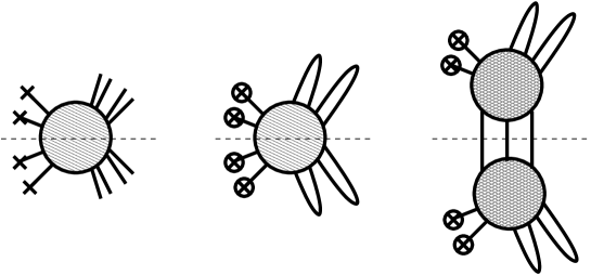
Figure 30: Two-particle-irreducibility of 2PI kernel: If the cut does not separate legs originating from the same original pair, it must cut at least three internal lines in the original diagram, since the latter originates from a 2PI closed graph in the 2PI effective action.

Appendix B Two-particle irreducibility of kernels

Here, we consider a key topological property of the 2PI kernels, namely that they are two-particle irreducible in the following sense. Consider a given 2PI kernel $\delta^{m+n}\Gamma_{\mbox{\scriptsize int}}/\delta G^{m}\delta\phi^{n}|_{\bar{G}}$ with $2m+n$ legs, as represented on the left of Fig. 30. This kernel arises from a closed 2PI diagram in the 2PI effective action. In order to split the latter into two disconnected parts one has to cut at least three lines. A similar analysis can be done for the kernel. The kernel has $n$ “single” legs, corresponding to derivatives with respect to the field $\phi$, and $m$ “pairs” of legs, arising from derivatives with respect to $G$. After the graph has been cut, part of these legs are attached to one piece and the rest to the other piece. In particular, if the cut does not separate two legs from a single pair, it must cut at least three internal lines in the diagram, as illustrated in Fig. 30. This follows from the two-particle irreducibility of the diagrams contributing to the 2PI effective action. As already emphasized in Refs. [16, 17], this property of 2PI kernels plays a crucial role in discussing renormalization (see also Sec. 2.3).

References

- [1] E. Braaten and R. D. Pisarski, Nucl. Phys. B 337 (1990) 569.
- [2] J. P. Blaizot, E. Iancu and A. Rebhan, in “Quark Gluon Plasma 3”, eds. R.C. Hwa and X.N. Wang, World Scientific, Singapore, 60 [arXiv:hep-ph/0303185].
- [3] J. P. Blaizot, E. Iancu and A. Rebhan, Phys. Rev. D 63 (2001) 065003 [arXiv:hep-ph/0005003]; J. O. Andersen and M. Strickland, Phys. Rev. D 71 (2005) 025011 [arXiv:hep-ph/0406163].
- [4] J. Berges, S. Borsányi, U. Reinosa and J. Serreau, Phys. Rev. D 71 (2005) 105004 [arXiv:hep-ph/0409123].
- [5] J. Berges and J. Serreau, “Progress in nonequilibrium quantum field theory,” in SEWM02, ed. M.G. Schmidt (World Scientific, 2003) [arXiv:hep-ph/0302210]; ibid. SEWM04, eds. K.J. Eskola, K. Kainulainen, K. Kajantje and K. Rummukainen (World Scientific) [arXiv:hep-ph/0410330].
- [6] J. Berges, “Introduction to nonequilibrium quantum field theory”, AIP Conf. Proc. 739 (2005) 3 [arXiv:hep-ph/0409233].
- [7] J. Berges and J. Cox, Phys. Lett. B 517 (2001) 369 [arXiv:hep-ph/0006160].
- [8] J. Berges, Nucl. Phys. A 699 (2002) 847 [arXiv:hep-ph/0105311].
- [9] F. Cooper, J. F. Dawson and B. Mihaila, Phys. Rev. D 67 (2003) 056003 [arXiv:hep-ph/0209051]; S. Juchem, W. Cassing and C. Greiner, Phys. Rev. D 69 (2004) 025006 [arXiv:hep-ph/0307353].
- [10] J. Berges, S. Borsányi and J. Serreau, Nucl. Phys. B 660 (2003) 51 [arXiv:hep-ph/0212404]; J. Berges, S. Borsányi and C. Wetterich, Phys. Rev. Lett. 93 (2004) 142002 [arXiv:hep-ph/0403234].
- [11] J. Berges and J. Serreau, Phys. Rev. Lett. 91 (2003) 111601 [arXiv:hep-ph/0208070].
- [12] G. Aarts and J. Berges, Phys. Rev. Lett. 88 (2002) 041603 [arXiv:hep-ph/0107129]; A. Arrizabalaga, J. Smit and A. Tranberg, JHEP 0410 (2004) 017 [arXiv:hep-ph/0409177].
- [13] M. Alford, J. Berges and J. M. Cheyne, Phys. Rev. D 70 (2004) 125002 [arXiv:hep-ph/0404059].
- [14] J. M. Luttinger and J. C. Ward, Phys. Rev. 118 (1960) 1417. G. Baym, Phys. Rev. 127 (1962) 1391.
- [15] J. Knoll, Y. B. Ivanov and D. N. Voskresensky, Annals Phys. 293 (2001) 126 [arXiv:nucl-th/0102044].
- [16] H. van Hees and J. Knoll, Phys. Rev. D 65 (2002) 025010 [arXiv:hep-ph/0107200]; Phys. Rev. D 65 (2002) 105005 [arXiv:hep-ph/0111193]; Phys. Rev. D 66 (2002) 025028 [arXiv:hep-ph/0203008].
- [17] J. P. Blaizot, E. Iancu and U. Reinosa, Phys. Lett. B 568 (2003) 160 [arXiv:hep-ph/0301201]; Nucl. Phys. A 736 (2004) 149 [arXiv:hep-ph/0312085].
- [18] J. M. Cornwall, R. Jackiw and E. Tomboulis, Phys. Rev. D 10 (1974) 2428.
- [19] S. R. Coleman, R. Jackiw and H. D. Politzer, Phys. Rev. D 10 (1974) 2491; W. A. Bardeen and M. Moshe, Phys. Rev. D 28 (1983) 1372; G. Amelino-Camelia and S. Y. Pi, Phys. Rev. D 47 (1993) 2356 [arXiv:hep-ph/9211211].
- [20] F. Cooper, B. Mihaila and J. F. Dawson, Phys. Rev. D 70 (2004) 105008 [arXiv:hep-ph/0407119]; F. Cooper, J. F. Dawson and B. Mihaila, arXiv:hep-ph/0502040.
- [21] G. Aarts, D. Ahrensmeier, R. Baier, J. Berges and J. Serreau, Phys. Rev. D 66 (2002) 045008 [arXiv:hep-ph/0201308].
- [22] J. Berges, S. Borsányi, U. Reinosa and J. Serreau, in preparation.
- [23] U. Reinosa, “Renormalization and gauge symmetry for 2PI effective actions,” in SEWM04, eds. K.J. Eskola, K. Kainulainen, K. Kajantje and K. Rummukainen (World Scientific) [arXiv:hep-ph/0411255].
- [24] C. De Dominicis and P. C. Martin, J. Math. Phys. 5 (1964) 14, ibid 31; R.E. Norton and J.M. Cornwall, Ann. Phys. (N.Y.) 91 (1975) 106; H. Kleinert, Fortschritte der Physik 30 (1982) 187; A.N. Vasiliev, “Functional Methods in Quantum Field Theory and Statistical Physics”, Gordon and Breach Science Pub. (1998).
- [25] J. Berges, Phys. Rev. D 70 (2004) 105010 [arXiv:hep-ph/0401172].
- [26] J. S. Schwinger, J. Math. Phys. 2 (1961) 407.
- [27] E. Braaten and E. Petitgirard, Phys. Rev. D 65 (2002) 041701 [arXiv:hep-ph/0106045]; Phys. Rev. D 65 (2002) 085039 [arXiv:hep-ph/0107118].
- [28] G. Aarts and J. M. Martinez Resco, Phys. Rev. D 68 (2003) 085009 [arXiv:hep-ph/0303216]; JHEP 0402 (2004) 061 [arXiv:hep-ph/0402192].
- [29] J. Serreau, JHEP 0405 (2004) 078 [arXiv:hep-ph/0310051].