Sleptonium at the linear collider and the slepton co-next-to-lightest supersymmetric particle scenario in gauge mediated symmetry breaking models

Abstract

We discuss the possibility of formation and subsequent detection of a supersymmetric bound state composed of a slepton–antislepton pair at the next linear collider. The Green function method is used within a non-relativistic approximation to estimate the threshold production cross-section of the $2P$ bound state. The parameter space of Gauge Mediated Symmetry Breaking (GMSB) models allow a particular scenario in which a charged slepton ($\widetilde{e}_{R},\widetilde{\mu}_{R}$ or $\widetilde{\tau}_{1}$) is the NLSP. Within this scenario the produced $2P$ bound-state decays, through a dipole transition, into the $1S$ ground-state with branching ratio $\approx 100\%$ emitting a very soft ($\approx 1$ MeV) photon which goes undetected. The spectroscopy of the $1S$-state shows that it decays into two photons with $Br\approx 0.5$ up to $m_{NLSP}\approx 1$ TeV. Thus NLSP sleptonium threshold production gives rise to the signal $e^{+}e^{-}\to 2P\to 1S+``soft\,\,\gamma"\to\gamma\gamma$ which when compared with the standard model two-photon process ($e^{+}e^{-}\to\gamma\gamma$ ) has a statistical significance ($SS$=signal/noise) which, at an energy offset from threshold of $E=20$ GeV, goes from $SS=11$ to $SS=2$ when the mass of the NLSP ranges in the interval $[100,200]$ GeV.

I Introduction

Despite the enormous success of the standard model (SM) of particle interactions based on the gauge group $SU(3)_{C}\otimes SU(2)_{L}\otimes U(1)_{Y}$ a large portion of current research efforts in the field of fundamental interactions is devoted to the study of signatures of physics beyond the SM. Between the possible alternatives to the standard model its minimal supersymmetric extension (MSSM) is one of the theories which has been extensively studied from both the purely theoretical and phenomenological aspects haberkane .

Supersymmetry, is the symmetry which relates fermions to bosons and, while appealing because of its potential of solving the hierarchy problem of the standard model, must of course be broken, and one of the major issues in supersymmetric theories is the pattern of supersymmetry breaking. There exist various possibilities to break supersymmetry. In mSUGRA models it is assumed that supersymmetry is broken at the Planck scale $M_{P}$ and is transmitted to the low-energy sector by gravitational interactions only mSUGRA . In gauge mediated symmetry breaking (GMSB) models supersymmetry is broken at relatively lower energy scales and is mediated by gauge interactions giudicerattazzi . Other possibilities consist of anomaly mediated symmetry breaking (AMSB). Here the SUSY-breaking occurs also in a hidden sector but it is transmitted to the visible sector via the super-Weyl anomaly AMSB .

Of course at this stage of experimental and theoretical investigations it is important to study in detail the phenomenological consequence of each scenario. Object of this work is the GMSB scenario whose theoretical basis and phenomenology has already been described in the literature, (see giudicerattazzi and references therein). In particular we recall that GMSB models are characterized by a rather peculiar superparticle mass spectrum. Indeed in these models the almost massless goldstino/gravitino, $\widetilde{G}$, is the lightest supersymmetric particle (LSP) and in addition to the neutralino $\chi^{0}_{1}$ next-to-lightest supersymmetric particle (NLSP) case, large fractions of the parameter space offer the possibility of having a charged NLSP which can be either the $\widetilde{\tau}_{1}$ or $\tilde{\ell}_{R}\,(\ell=e,\mu)$ .

In ambrosanio1 the phenomenology of the production of a pair of NLSP, within GMSB models, was discussed in the context of the Cern LEP2 collider. In particular it was found that in the stau NLSP or charged slepton NLSP cases typical signatures of NLSP pair production are $\tau^{+}\tau^{-}E\negthinspace\negthinspace\negthinspace/$, or $\ell^{+}\ell^{-}E\negthinspace\negthinspace\negthinspace/$ where the missing energy, $E\negthinspace\negthinspace\negthinspace/$, is due to the decay of the NLSP to the almost massless gravitino, $\widetilde{G}$, (LSP).

The object of this study is to propose a novel type of signature for the GMSB slepton NLSP scenario, assuming that the next LC will operate (at least initially) at energies approximatively in the neighborhood of the threshold of NLSP pairs. In this case if $\tilde{\ell}_{R}$ or $\widetilde{\tau}_{1}$ are the NLSP then the threshold production of sleptonium, a bound state of a slepton-antislepton pair, (smuonium or stauonium) in $e^{+}e^{-}$ collisions should be considered. It turns out that such bound state can give rise to the interesting signature of two photons and practically no missing energy. This signature has not been considered previously. Indeed the produced $2P$ state decays with branching ratio $\approx 100\%$ to the $1S$ state and a photon whose energy is related to the difference of the energy levels $E_{2P}-E_{1S}\approx 1$ MeV. In turn the $1S$ state decays mainly to two photons:

$$e^{+}e^{-} \to 2P\to 1S+\text{soft\ }\gamma$$ (1)

$$\phantom{2P\to}\,\,\,\buildrel|\over{\!}\!\rightarrow\gamma\gamma$$

The threshold production cross section of the $2P$ state in $e^{+}e^{-}$ collisions is computed using the Green function method within a non relativistic approximation. The decay widths of all open channels of the $2P$ and $1S$ states are also provided. It is concluded that the two-photon signature, when compared with the SM process $e^{+}e^{-}\to\gamma\gamma$, has a statistical significance ($SS=Signal/Noise$) which ranges in the interval from $11-3$ when the mass of the slepton ($m_{NLSP}$) is between $100$ and $300$ GeV.

The plan of the paper is as follows: section II provides a review of the GMSB supersymmetric model; in section III is discussed the criterion for formation of the supersymmetric bound state (sleptonium); section IV presents details of the decay channels of the $2P$ and $1S$ bound states; section V contains a description of the Green function method to estimate the threshold cross-section for the production of the $2P$ bound state; section VI presents a discussion of the statistical significance of the two-photon signature; finally section VII presents the conclusions.

II GMSB models

GMSB models of symmetry breaking are perhaps the most promising alternative to the SUGRA scheme where SUSY breaking takes place at the Planck mass and is then communicated to the low energy sector by gravitational interactions. In GMSB models supersymmetry breaking occurs at relatively lower energy scales and it is mediated by gauge interactions giudicerattazzi ; martin . One nice feature of these models is the automatic suppression of the SUSY contribution to FCNC and CP-violating processes.

In the simplest version such models are characterized by the introduction of messenger chiral superfield which contain quarks $\psi_{q},\psi_{\bar{q}}$, leptons $\psi_{\ell},\psi_{\bar{\ell}}$, scalar quarks $q,\bar{q}$ and scalar leptons $\ell,\bar{\ell}$ (messenger fields). All these particles must acquire very large masses as they have not been discovered. They do so by coupling to a gauge singlet chiral supermultiplet $X$ via the superpotential:

$$W_{mess}=\lambda_{2}X\ell\bar{\ell}+\lambda_{3}Xq\bar{q}$$ (2)

Then one assumes that the scalar component of $X$ and its auxiliary F-term acquire a vacuum expectation value (VEV) respectively denoted $\langle S\rangle$ and $\langle F_{S}\rangle$. Assuming for simplicity degeneracy of the couplings ($\lambda=\lambda_{2}=\lambda_{3}$) and absorbing the coupling $\lambda$ into $\langle S\rangle$ and $\sqrt{\langle F_{S}\rangle}$ by defining $M=|\lambda\langle S\rangle|$ and $F=|\lambda\langle F_{S}\rangle|$ the amount of SUSY breaking in the messenger sector i.e. the mass splitting of the scalar messenger states is found to be parametrized as:

$$m^{2}_{\text{mess. fermions}} = M^{2}$$

$$m^{2}_{\text{mess. scalars}} = M^{2}\pm F$$

$$\delta m^{2}_{\text{mess. scalars}} = 2F\qquad\to\qquad\delta m_{\text{mess. scalars}}=\frac{F}{M}=\Lambda\qquad(\,\hbox{if\ }F/M^{2}\ll 1)$$ (3)

SUSY breaking is thus apparent in the messenger sector, and is in turn communicated to the low energy sector (MSSM sparticles) through radiative quantum corrections. Gauginos (and scalar partners) acquire their masses, at the messenger scale $M$, through one loop (and two loop) Feynman diagrams where virtual messenger particles are exchanged dimopulos ; spmartin ; suspect :

$$M_{G}(M) = \frac{\alpha_{G}}{4\pi}\,\Lambda\,g(x)\,\sum_{m}\,N_{R}^{G}(m)\qquad G=U(1),SU(2),SU(3)$$ (4)

$${\widetilde{m}}_{s}^{2}(M) = 2\Lambda^{2}\,f(x)\,\sum_{G,m}\left(\frac{\alpha_{G}}{4\pi}\right)^{2}\,C_{R}^{G}(s)\,N_{R}^{G}(m)$$ (5)

In Eqs. (4,5) $x=F/M^{2}$, $m$ labels the messengers and $s$ the MSSM scalar; the functions $f(x)$ and $g(x)$, which reduce to $\approx 1$ when $x\to 0$ are explicitly given in ambrosanio1 ; suspect ; spmartin ; $N_{R}^{G}$ is the Dynkin index of the gauge representation under which the messenger superfields transform, defined by $TrT^{a}T^{b}=(N_{R}^{G}/2)\delta^{ab}$ the $T^{a}$ being the generators of the gauge group in the representation R; $C_{R}^{G}$ are the quadratic Casimir invariant of the same gauge group representation for the MSSM scalar field in question and, for the $\bm{N}$ of $SU(N)$), is defined by: $\sum_{a}T^{a}T^{b}=C^{SU(N)}_{\bm{N}}\bm{I}=(N^{2}-1)/2N\bm{I}$ . $N_{R}^{G}$ and $C_{R}^{G}$ turn out to be simple algebraic functions of the gauge couplings and the number $n_{\tilde{\ell}}$ and $n_{\tilde{q}}$ of messenger fields, see suspect ; ambrosanio1 for further details. From Eqs. (4,5) one also deduces that the scale of SUSY breaking felt in the messenger sector $\Lambda=F/M$ must be in the range

$$10\text{\ TeV}\leq\Lambda\leq 100\text{\ TeV}$$

in order to have sparticle masses in the range of $100$ GeV - 1 TeV.

A distinctive feature of GMSB models is the fact that the gravitino $\widetilde{G}$ may be very light. Indeed $m_{\widetilde{G}}$ is given by:

$$m_{\widetilde{G}}=m_{3/2}=\frac{F_{0}}{\sqrt{3}M_{P}^{\prime}}\approx\left(\frac{\sqrt{F_{0}}}{100\,\hbox{TeV}}\right)^{2}\,\,2.4\,\hbox{eV}$$ (6)

where $M_{P}^{\prime}=(8\pi G_{N})^{-1/2}=2.4\times 10^{18}$ GeV is the reduced Planck mass and $\sqrt{F_{0}}$ is the fundamental scale of super-symmetry breaking (SSB) which does not coincide with ${F}$, the scale of SUSY breaking felt by the messenger sector. The ratio $F/F_{0}$ depends on how SUSY breaking is communicated to the messenger sector. If the communication takes place via a direct interaction then $F/F_{0}$ is given by the corresponding coupling constant which by imposing perturbativity arguments can be shown to be smaller than 1 ambrosanio1 , thus giving ${F_{0}}>F$. If the communication of SUSY breaking takes place radiatively then $F/F_{0}$ is given by some loop factor and thus $F/F_{0}\ll 1$. It can easily be shown ambrosanio2 ; ambrosanio1 that $F_{0}$ is only subject to a lower bound which is:

$$\sqrt{F_{0}}\geq\Lambda$$ (7)

which is typically of the order of $10-100$ TeV.

Therefore the gravitino $\widetilde{G}$ turns out to be the lightest super-symmetric particle (LSP). In R conserving supersymmetry all sparticles eventually decay to the gravitino and in order to compute the decay widths one needs the interaction Lagrangian in the gravitino field which can be computed in the limit of global supersymmetry ( if $\sqrt{F_{0}}\ll M_{P}$) as the dominant gravitino interactions come from its spin $1/2$ component (the goldstino). It is therefore a good approximation to describe the gravitino LSP in terms of its spin $1/2$ goldstino component. Goldstino interactions contain derivative couplings suppressed by $1/F_{0}$:

$${\cal L}_{\text{int}}=-\frac{1}{F_{0}}\left(\bar{\psi_{L}}\gamma^{\mu}\gamma^{\nu}\partial_{\nu}\phi-\frac{i}{4\sqrt{2}}\bar{\lambda}^{a}\gamma^{\mu}\sigma^{\nu\rho}F^{a}_{\nu\rho}\right)\partial_{\mu}\widetilde{G}+h.c.$$ (8)

Sparticle phenomenology (production and decay) is strongly affected by the type of the next to lightest super-symmetric particle (NLSP). All sparticles will decay to a cascade leading to the NLSP which will in turn only decay to the gravitino $\widetilde{G}$ via $1/F_{0}$ interactions. Depending on the values of the parameters, the NLSP can be either the neutralino $\chi^{0}_{1}$, the stau $\widetilde{\tau}_{1}$, or in restricted regions of the parameter space the sneutrino ($\widetilde{\nu}$).
Of particular interest in this work is the case of a charged NLSP. In GMSB models the $\widetilde{\tau}_{1}$ is always the NLSP but in some circumstances it may happen that the mass of the ${\tilde{\ell}_{R}}$ be closer to $m_{\widetilde{\tau}_{1}}$ than the mass of the tau ($m_{\tau}$). If this is the case the ${\tilde{\ell}_{R}}=(\widetilde{e}_{R},\widetilde{\mu}_{R})$ act effectively as a NLSP since the decays ${\tilde{\ell}_{R}}\to\ell\widetilde{\tau}_{1}^{\pm}\tau^{\mp}$ are kinematically forbidden. This situation is referred to as slepton co-NLSP scenario, and it is more precisely defined by the condition:

$$m_{\tilde{\ell}_{R}}<\text{Min}\,[m_{\chi^{0}_{1}},m_{\widetilde{\tau}_{1}}+m_{\tau}]\,.$$ (9)

Within this scenario the sleptonium bound state of a pair of $\widetilde{\tau}_{1}$ or $\tilde{\ell}_{R}$ would be the lightest SUSY state to be produced in a laboratory. It is therefore interesting to explore throughly all possibilities to detect such a bound state at the next linear collider (NLC). In the following section we describe the spectroscopy in detail.
Within this scenario the NLSP $\tilde{\ell}=(\tilde{e}_{R},\tilde{\mu}_{R},\widetilde{\tau}_{1})$ total width is easily determined from Eq. (8):

$$\Gamma_{\tilde{\ell}}=\Gamma(\tilde{\ell}\to\ell\widetilde{G})=\frac{m^{5}_{\tilde{\ell}}}{16\pi F_{0}^{2}}=\left(\frac{m_{\tilde{\ell}}}{100\,\hbox{GeV}}\right)^{5}\left(\frac{100\,\hbox{TeV}}{\sqrt{F_{0}}}\right)^{4}\,2\times 10^{-3}\,\hbox{eV}$$ (10)

which will be used to establish a criterion for the formation of the bound state.

It should be noted that Eqs.(4,5) are to be considered as boundary conditions at the (high) messenger mass scale $M$. Low energy values of the parameters are to be obtained by running renormalization group equations (RGE) down to the electroweak scale. This process must of course ensure proper breaking of the electroweak (EW) symmetry. All this is achieved by the public domain code Suspect suspect , a software which allows for the possibility of choosing between mSUGRA, GMSB and AMSB models in addition to the general unconstrained MSSM. With Suspect is possible to perform a scan of the parameter space in order to select the scenario that one is interested in.

In its simplest version the GMSB model is characterized by a relatively small number of parameters:

$$M,\,\,\Lambda=\frac{F}{M},\,\,n_{\tilde{\ell}},\,\,n_{\tilde{q}},\,\,\tan(\beta),\,\,sign(\mu)$$ (11)

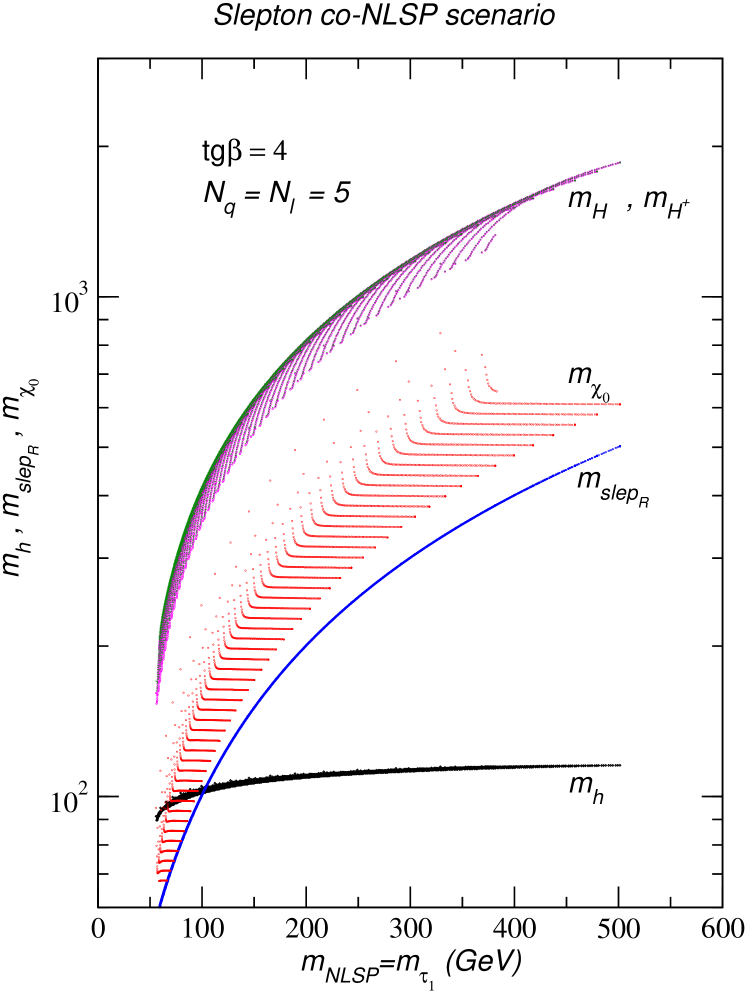
Figure 1: Sparticle spectrum in the slepton co-NLSP scenario. Only the masses of the sparticles which are relevant for our processes are shown as a function of the NLSP mass $m_{NLSP}=m_{\tilde{\tau_{1}}}$. What is shown here is a scan of the GMSB parameter space done imposing the slepton co-NLSP scenario condition given in Eq.(9).

In Fig. 1 we show the result of such a (numerical) study of the parameter space having fixed $\tan\beta=4$ and $n_{\tilde{\ell}}=n_{\tilde{q}}=5$. The scan has been performed on the plane $M,\Lambda$. In the figure we show the masses of $\tilde{\ell}_{R}(\approx m_{NLSP})$ and the higgs mass states entering into the spectroscopy of the bound state decays to be discussed in sec. IV. The mass of the neutralino is shown for completeness to confirm that it is heavier than $m_{\tilde{\ell}_{R}}$.

III Formation scenario

In this section we will review the creation of the bound state. For the SUSY case, our assumption will be that the creation of the bound state does not differ from the Standard Model case, as the relevant interaction is again driven by QED and is regulated by the mass of the constituent superparticles. A criterion for the formation of bound states we shall adopt is that NOI2 ; ME the formation can occur only if the level splitting, which depends upon the strength of the interaction among the (s)particles, is larger than the natural width of the would-be bound state. It means that the bound state is formed if the following condition is satisfied

$$\Delta E_{2P-1S}\geq\widetilde{\Gamma}$$ (12)

where $\Delta E_{2P-1S}=E_{2P}-E_{1S}$, and $\widetilde{\Gamma}$ is the width of the would–be sleptonium, which is twice the width of the single slepton $\widetilde{\Gamma}=2\Gamma_{\tilde{\ell}}$, as each slepton could decay in a fashion independent from the other. $\widetilde{\Gamma}$ is not the total decay width of the sleptonium bound state, as it includes only the single smuon decay modes and not the annihilation modes. It represents the minimal energy level spread necessary for bound state formation. If created, the bound state will in turn also have its own annihilation decay modes (as discussed in sec. IV).
For the case of a scalar bound state (sleptonium), we should consider the Coulombic two–body interaction

$$V(r)=-\frac{\alpha}{r}$$ (13)

where the coupling $\alpha$ is the usual fine structure constant of QED. With this position we are able to compute analytically the energy levels and the wavefunctions within a non relativistic approach. From

$$E_{n}=-\frac{m_{\tilde{\ell}}}{4}\;\frac{\alpha^{2}}{n^{2}}$$ (14)

one infers that

$$\Delta E_{2P-1S}=\frac{3}{16}\alpha^{2}m_{\tilde{\ell}}\approx 1\,\hbox{MeV}\,\left[\frac{m_{\tilde{\ell}}}{100\,\hbox{GeV}}\right]$$ (15)

Contrary to the QCD interaction case NOI the running of the coupling constant value is not very important, as the relevant scale given by the Bohr radius, $2/(m_{\tilde{\ell}}\alpha)$, is of $\mathcal{O}(1)\textrm{ GeV}^{-1}$. The $\Delta E$ value is thus determined only by the mass of the slepton. This has to be compared to the width of the would-be sleptonium $\widetilde{\Gamma}=2\Gamma_{\tilde{\ell}}$. Thus the requirement of formation, is obtained inserting Eq. 15 and Eq. 10 in Eq. 12:

$$\text{Bound State formation}\iff\sqrt{F_{0}}\geq 8\,m_{\tilde{\ell}}$$ (16)

We must emphasize that formation criterion adopted here for the sleptonium bound state is slightly less stringent than the one based on the revolution time, for which no bound states exist, if the revolution time, $t_{R}=2\pi r/v$, is larger than the lifetime of the rotating constituents, $\tau=1/\widetilde{\Gamma}$, as shown in ME .

In order to estimate the revolution time, we use the consequences of the virial theorem, which reads $\langle T\rangle=-\langle V\rangle/2$ for the average of kinetic and potential energies respectively. From the expression for the energy levels Eq. 14 we obtain the average speed of the constituent slepton, $\langle v^{2}\rangle=\alpha^{2}/(n^{2})$, that is

$$\langle v\rangle=\frac{\alpha}{n}$$ (17)

while the average distance of the constituent is given by

$$\langle r\rangle=r_{B}n^{2}\left[1+\frac{1}{2}\left(1-\frac{l(l+1)}{n^{2}}\right)\right]$$ (18)

for a Coulombic potential as in Eq. 13. Combining Eqs. 17 and 18 we compute the revolution time for the given state

$$t_{R}=\frac{4\pi}{m_{\tilde{\ell}}\alpha^{2}}n^{3}\left[1+\frac{1}{2}\left(1-\frac{l(l+1)}{n^{2}}\right)\right]\,.$$ (19)

Thus employing as a formation criterion that the bound state constituents life-time $\tau={1}/{\widetilde{\Gamma_{\tilde{\ell}}}}$ be larger than the revolution time leads us (see Eq. 10) to the inequality:

$$\text{ ($n,l$) Bound state formation}\iff\frac{16\pi{F_{0}}^{2}}{m_{\tilde{\ell}}^{5}}\geq\frac{4\pi}{m_{\tilde{\ell}}\alpha^{2}}n^{3}\left[1+\frac{1}{2}\left(1-\frac{l(l+1)}{n^{2}}\right)\right]\,.$$ (20)

We obtain two different conditions for the existence of the $1S$ and $2P$ bound states:

$$\text{$1S$ Bound state formation}\iff\sqrt{F_{0}}\geq 9.15\,m_{\tilde{\ell}}\,,$$ (21)

and

$$\text{$2P$ Bound state formation}\iff\sqrt{F_{0}}\geq 14.7\,m_{\tilde{\ell}}\,.$$ (22)

We thus realize that both formation criteria, Eq. (16) and Eq. (21,22) give comparable restrictions on the value of the fundamental scale of SUSY breaking $F_{0}$. In order to make sure that the bound state can be produced adopting both formation criteria the more conservative criterion of the two (that of the revolution time) is chosen.

For a slepton mass of the order of $100-200$ GeV the formation of the bound state(s) is assured on account of Eq. 7 ($\sqrt{F_{0}}\geq\Lambda$) and the fact that $\Lambda\approx 10-100$ TeV. We stress that the slepton mass $m_{\tilde{\ell}}$ is independent of the energy scale $\sqrt{F_{0}}$ which determines only the strength of the gravitino interactions.

IV Decay width and annihilation modes

The scalar bound state formed by a pair of slepton NLSP in an $e^{+}e^{-}$ collision will be a $2P$ state with several decay channels. It will decay into pair of standard model fermions. On the other end being formed by NLSP it will have only one decay channel into super-symmetric particles: it will decay (annihilate) into a pair of LSP, the almost massless gravitino (goldstino). Finally the $2P$ state will decay via dipole interactions to a $1S$ state emitting a photon. Before discussing these decay channels in detail we make an important remark. Within the slepton co-NLPS scenario the bound state can either be $\tilde{\ell}_{R}^{+}\tilde{\ell}_{R}^{-}$ or $\widetilde{\tau}_{1}^{+}\widetilde{\tau}_{1}^{-}$ as $\tilde{\ell}_{R}$ and $\widetilde{\tau}_{1}$ are nearly degenerate in mass. When discussing the decay of the bound state however the case of the $\widetilde{\tau}_{1}$ is somewhat complicated by the fact that left-right mixing must be taken into account and diagrams, which are absent in the $\tilde{\ell}_{R}$ only case, have to be included. Therefore as a first step we consider only a bound state of $\tilde{\ell}_{R}=\widetilde{e}_{R},\widetilde{\mu}_{R}$. The case of the $\widetilde{\tau}_{1}$ shall be treated on a separate work.
In addition while $\widetilde{\mu}$ and $\widetilde{\tau}$ cross sections are universal $\widetilde{e}$ pair production suffers from destructive interference effects between s-channel and t-channel diagrams in the parameter region relevant for GMSB models (moderate values of $\tan\beta$) GFgiudice . For this reason in the following we shall consider only the the bound state of $\widetilde{\mu}_{R}$ (smuonium).

The calculation of the partial widths of the decay of the sleptonium bound state ($\tilde{\ell}_{R}^{+}\tilde{\ell}_{R}^{-}$), i.e. $2P\to X$ or $1S\to X$, is done by relating the amplitude ${\cal M}(B\to X)$ to that of the process $\tilde{\ell}_{R}^{+}\tilde{\ell}_{R}^{-}\to X$ via a non relativistic model of the bound state peskin :

$${\cal M}(B\to X)=\sqrt{2M_{B}}\,\int\frac{d^{3}\bm{k}}{(2\pi)^{3}}\widetilde{\psi}^{*}(\bm{k})\,\frac{1}{2m_{{\tilde{\ell}}_{R}}}\left[{\cal M}\left(\tilde{\ell}_{R}^{+}\tilde{\ell}_{R}^{-}\to X\right)\right]_{s\to 2m_{{\tilde{\ell}}_{R}}}$$ (23)

$\widetilde{\psi}(\bm{k})$ being the Fourier transform of the hydrogen-like wave function of the non relativistic bound state. The amplitude ${\cal M}\left(\tilde{\ell}_{R}^{+}\tilde{\ell}_{R}^{-}\to X\right)$ will in general be described by one or more tree-level Feynman diagrams an thus its threshold behaviour $s\to 2m_{{\tilde{\ell}}_{R}}$ may be inferred. Thus for each decay one writes down the amplitudes of the contributing Feynman diagrams and then extracts the dependence of the full amplitude on $\bm{k}$, the momentum of the constituents sleptons which is assumed to be smaller with respect to the mass of the sleptons, $|\bm{k}|\ll m_{\tilde{\ell}_{R}}$, giving $\sqrt{s}=2\sqrt{m_{\tilde{\ell}_{R}}^{2}+|\bm{k}|^{2}}\approx 2m_{\tilde{\ell}_{R}}\left(1+|\bm{k}|^{2}/m_{\tilde{\ell}_{R}}^{2}\right)$.

In $S$-wave decays one obtains an amplitude whose first term in the momentum expansion is a constant. Then the $\bm{k}$ integration in Eq. (23) gives the wavefunction evaluated at the origin: $\int d^{3}{\bm{k}}/(2\pi)^{3}\widetilde{\psi}^{*}(\bm{k})={\psi}^{*}(0)$. In $P$-wave decays one obtains instead an amplitude whose first term in the $\bm{k}$ momentum expansion is linear. Then the $\bm{k}$ integration in Eq. (23) gives the gradient of wavefunction evaluated at the origin: $\int d^{3}{\bm{k}}/(2\pi)^{3}\bm{k}_{i}\widetilde{\psi}^{*}(\bm{k})=\nabla_{i}{\psi}^{*}(0)$.

For further details see for example JACKSON ; drees . In passing we note that in the process of comparing the amplitude of the two photon decay mode of the $1S$ state we find an extra factor of 2 in Eqs. (A1) and (A2) of ref. drees , relative to stoponium decay into two photons and two gluons, a remark that had already been made in ref. gorbunov .

IV.1 Decay channels of the $\bm{2P}$ state

Decay into gravitinos: $2P\to\widetilde{G}\widetilde{G}$
The process is described by a $t$-channel exchange of a lepton of the same flavour of the bound state. The decay width is:

$$\Gamma(2P\to\widetilde{G}\widetilde{G})=\frac{1}{32\pi^{2}}\,\frac{|R{{}^{\prime}}_{2P}(0)|^{2}}{M_{B}^{4}}\,\left(\frac{M_{B}}{\sqrt{F_{0}}}\right)^{8}$$ (24)

Annihilation into neutrinos: $2P\to\nu_{\ell}\bar{\nu_{\ell}},\,\,(\ell=e,\mu,\tau)$.
This is the simplest decay annihilation channel which takes place only through the Z boson. In this case there are no $t$-channel exchange graphs, even when the flavour of the neutrinos is the same of the sleptonium bound state, since only left s-leptons ($\widetilde{\ell}_{L}$) do couple charginos and neutrinos. The decay width is:

$$\Gamma(2P\to\nu_{\ell}\bar{\nu_{\ell}})=\,{\alpha^{2}}\,\frac{|R{{}^{\prime}}_{2P}(0)|^{2}}{M_{B}^{4}}\,\frac{1}{\cos^{4}\theta_{W}}\,f(r_{Z},\epsilon_{Z})$$ (25)

where $f(x,y)={1}/[{(1-x^{2})^{2}+(xy)^{2}}]$ and $r_{Z}=M_{Z}/M_{B};\epsilon_{Z}=\Gamma_{Z}/M_{B}$.

Annihilation into charged standard model fermions $2P\to f\bar{f}$
First we consider the case that $f$ is either a quark or a lepton ($\ell^{\prime}\neq\ell$), $\ell$ being the flavour of the sleptonium bound state. When this is the case the decay is through the annihilation into $\gamma$ and $Z$-boson only: there are no $t$ channel exchange diagrams. The decay width is then:

$$\Gamma(2P\to f\bar{f}) = 8\,C_{F}\,\alpha^{2}\frac{|R_{2P}^{\prime}(0)|^{2}}{M_{B}^{4}}\sqrt{1-4\frac{m_{f}^{2}}{M_{B}^{2}}}\left(1-\frac{m_{f}^{2}}{M_{B}^{2}}\right)\,$$ (27)

$$\times\left[Q_{f}^{2}+\frac{c_{V}^{2}+c_{A}^{2}}{4\cos^{4}\theta_{W}}\,f(r_{Z},\epsilon_{Z})+Q_{f}\frac{c_{V}}{\cos^{2}\theta_{W}}(1-r_{Z}^{2})\,f(r_{Z},\epsilon_{Z})\right]$$

where: $C_{F}=3$ for quarks while $C_{F}=1$ for leptons; $Q_{f}$ is the charge of the fermion in units of $+e$; $c_{V}$ and $c_{A}$ are respectively the vector and axial coupling of the fermion to the Z-boson: $c_{V}^{f}=T^{3}_{f}-2Q_{f}\sin^{2}\theta_{W}$ and $c_{A}^{f}=T^{3}_{f}$; $m_{f}$ is the mass of the fermion; the function $f(x,y)$ is the same that appears in Eq.(25). One might notice that the above formula reduces to the decay width into neutrinos by taking the limit $Q_{f}=0$ and $m_{f}=0$. It also reduces to the formula of refs.c.nappi ; VANROYEN : $R_{2P}^{\prime}(0)$ being the derivative of the radial part of the wave function at the origin, and $M_{B}=2m_{\tilde{\ell}}$ is the bound state mass.
When the fermion $f$ is the lepton $\ell$ of the same flavour of the slepton $\tilde{\ell}_{R}$ forming the bound state Eq. (27) is to be replaced by the following (the lepton $\ell$ is assumed mass-less):

$$\Gamma(2P\to\ell^{+}\,{\ell^{-}}) = 8\alpha^{2}\frac{|R_{2P}^{\prime}(0)|^{2}}{M_{B}^{4}}\,\left[1+\frac{1/2+4\sin^{4}\theta_{W}-2\sin^{2}\theta_{W}}{4\cos^{4}\theta_{W}}\,f(r_{Z},\epsilon_{Z})\right.$$ (30)

$$\phantom{xxxxxxxxxxx}\left.+\frac{1/2-2\sin^{2}\theta_{W}}{\cos^{2}\theta_{W}}(1-r_{Z}^{2})\,f(r_{Z},\epsilon_{Z})\right.$$

$$\phantom{xxxxxxxxxxx}\left.+\frac{G^{2}}{2}-G+\sin^{2}\theta_{W}G\frac{1-r_{Z}^{2}}{\cos^{2}\theta_{W}}f(r_{Z},\epsilon_{Z})\,\right]$$

where the form factor $G$ describes the diagram of the $t-$channel exchange of a virtual neutralino. Assuming that the neutralino is mostly bino one has the simplified expression with:

$$G=\frac{4M_{B}^{2}}{M_{B}^{2}+4m^{2}_{\chi^{0}}}$$

Dipole decay into the ground state and a photon, $2P\to 1S+\gamma$
The decay to the ground state takes place through a transition with emission of a photon. This transition can be computed in the long wavelength approximation. Indeed the photon momentum $Q=\Delta E_{2P-1S}$, see Eq. (15), and the bound state dimension (Bohr radius) $r_{B}=2/(m_{\tilde{\ell}}\alpha)$ satisfy the relation

$$Qr_{B}=\frac{6}{16}\alpha\approx 2\times 10^{-3}<<1$$

which is the condition that makes the dipole approximation suitable. Then a standard quantum mechanics calculation gives davydov :

$$\Gamma(2P\to 1S+\gamma)=\frac{4}{9}\;\alpha(\Delta E_{2-1})^{3}(D_{2,1})^{2}$$ (31)

where $\Delta E_{2-1}$ is the energy of the emitted photon, and

$$D_{2,1}=\langle 2P|r|1S\rangle=\int_{0}^{\infty}drr^{3}R_{1S}(r)R_{2P}(r)$$ (32)

is the dipole moment (see NOI and references therein). The wave functions to be used are the one of the Coulombic model, given by

$$R_{1S}(r) = 2\left(\frac{1}{r_{B}}\right)^{3/2}\exp\left(-\frac{r}{r_{B}}\right)$$ (33)

$$R_{2P}(r) = \frac{1}{\sqrt{3}}\left(\frac{1}{2r_{B}}\right)^{3/2}\frac{r}{r_{B}}\;\exp\left(-\frac{r}{2r_{B}}\right)$$ (34)

where $r_{B}$ is the Bohr radius defined as $r_{B}=2/(m_{\tilde{\ell}}\alpha)=4/(M_{B}\alpha)$. Using the above wavefunctions one obtains the following expressions for the dipole decay mode:

$$\Gamma(2P\to 1S+\gamma) = \alpha^{5}M_{B}\frac{64}{6561}\,\approx\,\alpha^{5}M_{B}\,10^{-2}$$ (35)

Then we have to compute the total decay width to fermions:

$$\Gamma({2P\to fermions})=\sum_{f=q,\ell,\ell^{\prime}}\Gamma(2P\to f\bar{f})+\Gamma(2P\to\widetilde{G}\widetilde{G})$$ (36)

The derivative in the origin of the radial wavefunction of the $2P$ state is easily computed and it follows that: ${|R_{2P}^{{}^{\prime}}(0)|^{2}}/{M_{B}^{4}}={\alpha^{5}M_{B}}/{24576}$. Inserting the results of the Eqs. (24,25,27,30) into Eq. (36) one obtains:

$$\Gamma(2P\to fermions)={\alpha^{5}M_{B}}\,k\,10^{-5}$$ (37)

where $k$ is a numerical constant of order unity with a mild dependence on the mass of the bound state $M_{B}$, the fundamental scale of SUSY breaking $\sqrt{F_{0}}$ and the mass of the neutralino $m_{\chi^{0}}$. It then follows that the branching ratio of the dipole decay is $Br(2P\to 1S+\gamma)=100\%$ to within one part in $10^{3}$. For all practical purposes the $2P$ state will decay with probability $1$ to the ground state $1S$ emitting one photon with an energy of a few MeV.

IV.2 Decay channels of the $\bm{1S}$ ground state

Decay into two photons.
In this case since the photon is described by transversely polarized states, in the non-relativistic limit the t- and u-channel diagrams do not contribute and only the sea-gull diagram survives. The decay width is given by:

$$\Gamma(1S\to\gamma\gamma)=2\,\alpha^{2}\frac{|R_{1S}(0)|^{2}}{M_{B}^{2}}$$ (38)

Decay into $\gamma Z$.
Again the fact that the photon does not have longitudinal polarization states selects, in the non relativistic limit, only the sea-gull diagram. The decay width is given by:

$$\Gamma(1S\to\gamma Z)=4\,\alpha^{2}\,\frac{\sin^{2}\theta_{W}}{\cos^{2}\theta_{W}}\frac{|R_{1S}(0)|^{2}}{M_{B}^{2}}\,\left(1-\frac{M_{Z}^{2}}{M_{B}^{2}}\right)$$ (39)

Decay into $ZZ$.
Here there are four diagrams that give non zero contribution. The diagram with a $\tilde{\ell}_{R}$ in the $t$-channel and its exchange contribute only for the longitudinal polarization states of the Z gauge boson. The sea-gull term ($\tilde{\ell}_{R}\,\tilde{\ell}_{R}-ZZ$) and the $s$-channel higgs exchange give non zero contribution for all type of the Z boson polarization. The decay width is found to be:

$$\Gamma({1S\to ZZ}) = \frac{\alpha^{2}}{2}\,\tan^{4}\theta_{W}\,\frac{|R_{1S}(0)|^{2}}{M_{B}^{2}}\,\beta_{Z}\left\{|F+2|^{2}\left(3-\frac{M_{B}^{2}}{M_{Z}^{2}}+\frac{1}{4}\frac{M_{B}^{4}}{M_{Z}^{4}}\right)\right.$$ (40)

$$\phantom{xxxx}\left.+G^{2}\left(\frac{1}{4}\frac{M_{B}^{2}}{M_{Z}^{2}}-1\right)^{2}-2G\left(\Re e{F}+2\right)\left[1-\frac{3}{4}\frac{M_{B}^{2}}{M_{Z}^{2}}+\frac{1}{8}\frac{M_{B}^{4}}{M_{Z}^{4}}\right]\right\}$$

where:

$$\beta_{Z} = \sqrt{1-4\frac{M_{Z}^{2}}{M_{B}^{2}}}$$

$$F = \sum_{i=1,2}\,c_{i}\,\frac{M_{Z}^{2}}{M^{2}_{B}-M_{H_{i}}^{2}+i\Gamma_{H_{i}^{0}}M_{H_{i}^{0}}}$$

$$G = 4M_{B}^{2}/(M_{B}^{2}-2M_{Z}^{2})$$

$$c_{1} = \cos(\beta-\alpha)\cos(\beta+\alpha)/\sin^{2}\theta_{W}$$

$$c_{2} = -\sin(\beta-\alpha)\sin(\beta+\alpha)/\sin^{2}\theta_{W}$$

while $F$ is a form factor arising from the diagrams with $s$-channel Higgs exchange, $G$ arises from the $t$-channel $\tilde{\ell}_{R}$-exchange diagrams.
Decay into $W^{+}W^{-}$.
In this case the $t$-channel exchange of a sneutrino is absent (no $\widetilde{\nu}_{R}$) as well as the sea-gull term ($\tilde{\ell}_{R}\,\tilde{\ell}_{R}-WW$), and only the $s$-channel Higgs contribution is present. The partial decay width is:

$$\Gamma({1S\to W^{+}W^{-}})=\frac{\alpha^{2}}{2}\,\frac{|R_{1S}(0)|^{2}}{M_{B}^{2}}\,|F^{\prime}|^{2}\,\beta_{W}\,\left[3-\frac{M_{B}^{2}}{M_{W}^{2}}+\frac{1}{4}\frac{M_{B}^{4}}{M_{W}^{4}}\right]\,$$ (41)

where:

$$\beta_{W} = \sqrt{1-4\frac{M_{W}^{2}}{M_{B}^{2}}}$$

$$F^{\prime} = \sum_{i=1,2}\,c_{i}\,\frac{M_{Z}^{2}}{M^{2}_{B}-M_{H_{i}^{0}}^{2}+i\Gamma_{H_{i}^{0}}M_{H_{i}^{0}}}$$

$$c_{1} = \cos(\beta-\alpha)\cos(\beta+\alpha)$$

$$c_{2} = -\sin(\beta-\alpha)\sin(\beta+\alpha)$$

Decay into $hh$.
Within the minimal supersymmetric version of the higgs sector there are five higgs states: three neutrals, ($h,H,A$) and two charged, ($H^{\pm}$). Here we consider only the decay of the $1S$ state into a pair of the lightest Higgs states ($h$). The process receives contribution from three diagrams: a) $t-$channel $\tilde{\ell}_{R}$-exchange; b) $s$-channel higgs exchange $(h,H)$ [CP invariance forbids $s$-channel exchange of $A$]; c) sea-gull term $\tilde{\ell}_{R}\tilde{\ell}_{R}-hh$. There are no diagrams with $s$-channel exchange of $Z$ since Bose symmetry forbids $ZH_{i}^{0}H_{i}^{0}$ couplings. The decay width is found to be:

$$\Gamma({1S\to hh})=\frac{\alpha^{2}}{2\cos\theta_{W}^{4}}\,\frac{|R_{1S}(0)|^{2}}{M_{B}^{2}}\,\beta_{h}\,\left|Y\right|^{2}$$ (42)

$$\beta_{h} = \sqrt{1-4\frac{M_{h}^{2}}{M_{B}^{2}}}$$

$$Y = \sum_{i=1,2}c_{i}\frac{M_{Z}^{2}}{M_{B}^{2}-M_{H_{i}^{0}}^{2}+i\Gamma_{H_{i}^{0}}M_{H_{i}^{0}}}-\frac{\cos(2\alpha)}{2}+\sin^{2}\theta_{W}\sin^{2}(\alpha+\beta)\frac{4M_{Z}^{2}}{2M_{h}^{2}-M_{B}^{2}}$$

$$c_{2} = (3/2)\sin^{2}(\beta+\alpha)\cos(2\alpha)$$

$$c_{1} = 2\sin(2\alpha)\sin(\alpha+\beta)\cos(\alpha+\beta)-\cos(2\alpha)\cos^{2}(\alpha+\beta)$$

In Fig. 2 the partial widths of the various decay channels of the $1S$ state are shown with respect to the bound state mass $M_{B}$. We see that the two photon channel always dominates. The branching ratio $Br(1S\to\gamma\gamma)$ is $Br=0.65$ at $m_{\tilde{\ell}_{R}}=100$ GeV and $Br\approx 0.52$ up to $m_{\tilde{\ell}_{R}}=1000$ GeV, as shown in Fig. 3.

The detection of the $P$ wave bound state is therefore associated to the emission of a soft photon plus a subsequent emission of two hard photons given by the decay of the scalar ground state.

V cross section

V.1 Slepton pair production cross-section

We use the notation $\alpha_{\tilde{\ell}}=(3\tan\theta_{W}-\cot\theta_{W})/4$ and $\beta_{\tilde{\ell}}=(\tan\theta_{W}+\cot\theta_{W})/4$. The production cross section for scalar sleptons - except for selectrons - is given by TATA

$$\sigma(e^{+}e^{-}\to\tilde{\ell}_{i}^{+}\tilde{\ell}_{i}^{-})=\frac{\pi\alpha^{2}}{12}\beta^{3}\left[\frac{4}{s}+\frac{A_{\tilde{\ell}_{i}}^{2}(\alpha_{\tilde{\ell}}^{2}+\beta_{\tilde{\ell}}^{2})s-4\alpha_{\tilde{\ell}}A_{\tilde{\ell}_{i}}(s-M_{Z}^{2})}{(s-M_{Z}^{2})^{2}+(M_{Z}\Gamma_{Z})^{2}}\right]$$ (43)

with $i=L,R$; $A_{\tilde{\ell}_{L}}=2(\alpha_{\tilde{\ell}}-\beta_{\tilde{\ell}})$ or $A_{\tilde{\ell}_{R}}=2(\alpha_{\tilde{\ell}}+\beta_{\tilde{\ell}})$ for left- and right- handed sleptons respectively.

It is useful to write down this expression of the $P$ wave cross section in the following manner:

$$\sigma(e^{+}e^{-}\to\tilde{\ell}\overline{\tilde{\ell}})=\frac{4\alpha^{2}}{3s}\;\beta^{3}\;d(s)$$ (44)

V.2 Bound state production cross-section

We shall write the threshold cross section of the bound state in terms of its Schrödinger Green function. To review briefly the method, explained in more detail in ME2 , consider the bound state described by a Schrödinger equation with a suitable potential $V(\bm{x})$. The threshold cross section is then proportional to the imaginary part of derivative taken at the origin of the $P$ wave Green function of the problem $G_{1}(\bm{x},\bm{y},E)$. $E$ is the energy displacement from threshold, and the finite width of the state is taken into account by the substitution $E\to E+i\Gamma$.

The cross section for the production of a bound state can be normalized to the QED process $e^{+}e^{-}\to\mu^{+}\mu^{-}$:

$$R = \frac{\sigma(e^{+}e^{-}\to 2P)}{\sigma(e^{+}e^{-}\to\mu^{+}\mu^{-})}$$ (45)

$$= \frac{4\pi}{m^{4}_{\tilde{\ell}}}\;d(s)\;{\Im}m\left[{\sf Tr}\left.\frac{\partial}{\partial{x_{i}}}\,\frac{\partial}{\partial{y}_{j}}\,G^{(1)}(\bm{x},\bm{y},E)\,\right]\right|_{\bm{x}=0,\bm{y}=0}$$ (46)

where $d(s)$ is the usual expression of the Born cross section for the process $e^{+}e^{-}\to\tilde{\mu}\overline{\tilde{\mu}}$ written in Eq. (43). In our investigation the interaction among the two superpartners is driven by a Coulombic interaction with

$$V(r)=-\frac{\alpha}{r}$$ (47)

Adapting the notations of PP we set $E=\sqrt{s}-2m_{\tilde{\mu}}$ as the energy displacement from threshold, $k^{2}=-m_{\tilde{\mu}}E$, the wavelength $\lambda=9m\alpha/8$, and the wave number $\nu=\lambda/k$. Now the explicit form for the $\ell=1$ Green function $G_{1}$ of Eq. (46) takes the form

$$G_{1}(0,0,k)=\frac{m_{\tilde{\mu}}}{36\pi}\lambda\left\{2(k^{2}-\lambda^{2})\left[\frac{k}{2\lambda}+\ln\left(\frac{k}{\mu_{f}}\right)+2\gamma_{E}-\frac{11}{6}+\psi_{1}(1-\nu)\right]+\frac{k^{2}}{2}\right\}$$ (48)

$\gamma_{E}$ is Euler’s constant, $\psi_{1}$ is the digamma function, logarithmic derivative of the $\Gamma$ function and $\mu_{f}$ is a soft scale estimated from a relativistic framework (see ME2 and references therein). The derivative of Eq. (48) needed for computing the cross section Eq. (46) has a simple expression, as we have

$${\sf Tr}\,\left.\frac{\partial}{\partial{x}_{i}}\,\frac{\partial}{\partial{y}_{j}}\,G^{(1)}(\bm{x},\bm{y},k)\right|_{\bm{x}=0,\bm{y}=0}=9G^{(1)}(0,0,k)\,\,.$$ (49)

From Eq. (48) one can readily notice that the leading term in the cross section Eq. (46) for large $E$ is given by $k^{3}$, whereas the peaks of the bound state energy levels are determined by the digamma function in $\nu$.

The Green function method is a non-relativistic procedure. We have therefore to ensure that the velocity of the sleptonium constituents is low enough in order to keep relativistic corrections negligible. Starting from the parametrization of the center of mass energy $\sqrt{s}=2m_{\tilde{\ell}}+E$ and assuming an upper value for the constituent velocity $\beta_{MAX}$ we obtain an upper bound for the energy offset from threshold

$$E\leq E_{MAX}=m_{\tilde{\ell}}\beta_{MAX}^{2}$$ (50)

by means of a series expansion in $E$. This relation translates to the maximal allowed value of Lorentz boost parameter $\gamma$

$$\frac{E_{MAX}}{m_{\tilde{\ell}}}=\frac{\gamma^{2}_{MAX}-1}{\gamma^{2}_{MAX}}.$$ (51)

We thus define the non-relativistic domain by imposing that the value of $\gamma$ differs from $1$ by less than $\approx 10$%. This then gives $\beta_{MAX}\approx 1/\sqrt{5}$ and therefore, for a slepton mass $m_{\tilde{\ell}}=100$ GeV, an energy offset from threshold equal to $E_{MAX}=20$ GeV. From eq. 50 one could also observe that the acceptable (non-relativistic) threshold energy range increases when larger values of the constituent mass are considered.

In addition we emphasize that the entire procedure of treating the bound state breaks down away from threshold, independently of where relativistic corrections may become important.

VI Results and discussion

We shall analyse the threshold behaviour of cross section for a range of masses and SUSY parameters for which the bound state formation is envisaged, as discussed in section IV. Following ME2 we observe that the relevant region for our analysis is the one above threshold, i.e. for $E>0$. In fact the region below threshold, $E<0$, is characterised by peaks in the cross section located at the discrete energy values of bound states. Their width is given by the annihilation modes which, as shown in IV is of the order of the eV at most. From eq. (14) one can estimate the separation of the discrete peaks. They merge when the peaks are not distant enough

$$\frac{m}{4}\alpha^{2}\left[\frac{1}{n^{2}}-\frac{1}{(n+1)^{2}}\right]\sim\Gamma$$ (52)

The last resolved peak has a quantum number $n$ given by

$$\frac{2n+1}{n^{2}(n^{2}+1)}\sim\frac{4\Gamma}{m\alpha^{2}}\ll 1$$ (53)

Due to the beam energy spread of the collider, much larger than a few eV of the natural width of the state and of the order of few GeV TESLA this structure cannot be observed. The difference from the usual Born cross section results therefore should be sought for $E>0$.

The effect of the bound state to the cross section at threshold is to accumulate and merge the peaks towards the $E=0$ value, giving a larger result than the naive Born cross section, as we could see in Figs. 4 and 5.

VI.1 The signal and its statistical significance

Let us now discuss in some detail the signal

$$e^{+}e^{-}\to 2P\to 1S+\text{``soft $\gamma$''}\to\gamma\gamma$$ (54)

where the soft photon is assumed to be undetected since its energy is of only 1 or 2 MeV, see Eq. 15. Indeed it is known tesla2 that the photon energy resolution of the calorimetric detector is, for low-energy photons, of the type $\delta E/E\approx 0.11/\sqrt{E/\text{GeV}}$ which implies that $\delta E/E\approx 1$ for $E=10$ MeV. Therefore the 1-2 MeV soft photon of our signal will surely be much below the energy resolution and will be undetected.

The observed final state is therefore two hard back-to-back photons. This two photon signal of the production of the $2P$ sleptonium bound state is to be compared with the QED two photon process $e^{+}e^{-}\to\gamma\gamma$ which is expected to be the dominant background. The number of events of the signal can thus be estimated by:

$$N_{sign.}={\cal L}\sigma_{B}\,Br(2P\to 1S+\gamma)\,Br(1S\to\gamma\gamma)$$ (55)

where $\sigma_{B}$ is the threshold cross section for the production of the bound state computed with the Green function method. Given the fact that $Br(2P\to 1S+\gamma)\approx 1$ we have

$$N_{sign.}={\cal L}\sigma_{B}\,Br(1S\to\gamma\gamma)$$ (56)

The statistical significance $SS$ of the signal can thus be estimated by:

$$SS=\frac{N_{signal}}{\sqrt{N_{background}}}=\frac{{\cal L}\sigma_{B}\,Br(1S\to\gamma\gamma)}{\sqrt{{\cal L}\sigma_{\gamma\gamma}}}$$ (57)

A comment is in order at this point. The two-photon decay of the bound state is isotropic in the rest frame of the bound state which however will approximatively coincide with the laboratory frame as we are assuming threshold production with $E\leq 20$ GeV. The distortion introduced in the laboratory system when boosting the isotropic distribution of the two-photon signal from the bound state rest frame depends on the $\beta(M)$ of the bound state. Indeed in the bound state rest frame let $\theta^{*}$ be the angle of the direction of the two outgoing (back-to-back) photons:

$$\frac{d\sigma_{B}}{d\cos\theta^{*}}=\frac{\sigma_{B}(s)}{4}$$ (58)

where the phase space integration has been reduced of a factor of $1/2$ due to the identical particles in the final state. The distribution can be boosted landau to the laboratory frame where the bound state has a velocity $\beta(s),\sqrt{s}=2m_{\tilde{\ell}}+E$, $E$ being the offset from the threshold:

$$\frac{d\sigma_{B}}{d\cos\theta}=\frac{\sigma_{B}(s)}{4}\frac{1-\beta^{2}}{(1-\beta\cos\theta)^{2}}$$ (59)

where now $\theta$ is the direction of the photon in the laboratory frame.
On the other end the angular differential distribution of the photons for the QED process $e^{+}e^{-}\to\gamma\gamma$ is given by:

$$\frac{d\sigma_{\gamma\gamma}}{d\cos\theta}=\frac{\pi\alpha^{2}}{s}\frac{1+\cos^{2}\theta}{1-\cos^{2}\theta}$$ (60)

which is symmetric and peaked in the forward and backward directions. Again a factor of $1/2$ has been included in the phase-space factor due to the identical particles of the final state. Applying an angular cut in the forward and backward directions

$$\theta_{0}<\theta<\pi-\theta_{0}$$

it is possible to suppress the background in such a way as to obtain an interesting statistical significance. We define a cut dependent statistical significance:

$$SS(\theta_{0})=\frac{N_{sig}(\theta_{0})}{\sqrt{N_{back}(\theta_{0})}}=\frac{{\cal L}\times Br(1S\to\gamma\gamma)\int_{\theta_{0}}^{\pi-\theta_{0}}\,\sin\theta d\theta\,(d\sigma_{B}/d\cos\theta)}{\sqrt{{\cal L}\int_{\theta_{0}}^{\pi-\theta_{0}}\,\sin\theta d\theta\,(d\sigma_{\gamma\gamma}/d\cos\theta)}}$$ (61)

Defining $z_{0}=\cos\theta_{0}$ one easily finds:

$$SS(z_{0})=\frac{\sqrt{\cal L}\sigma_{B}(s)}{\sqrt{2\pi\alpha^{2}/s}}\times Br(1S\to\gamma\gamma)\times\frac{\frac{1-\beta^{2}}{1-\beta^{2}z_{0}^{2}}\frac{z_{0}}{2}}{\sqrt{\log\left(\frac{1+z_{0}}{1-z_{0}}\right)-z_{0}}}$$ (62)

The statistical significance as function of the angular cut is shown in Figs. 6 and 7. We observe a very mild dependence on $\theta_{0}$ apart from values of $\theta_{0}\approx 0$ and $\theta_{0}\approx\pi/2$. For these limiting values the statistical significance approaches zero. When $\theta_{0}\to 0$, $SS(\theta_{0})\to 0$ since the QED two photon background total cross-section is divergent. On the other hand when $\theta_{0}\to\pi/2$ one is integrating over a region of phase space of vanishing measure so that both cross sections vanish as $z_{0}=\cos\theta_{0}$ in this limit. One notices that for values of $\theta_{0}$ in the range $0.4\leq\theta_{0}\leq 0.8$ the statistical significance is almost constant and ranges from $SS\approx 4$ to $SS\approx 11$ for values of the energy offset respectively of $E=10$ GeV and $E=20$ GeV, and for a fixed slepton mass $m_{\tilde{\ell}_{R}}=100$ GeV.

In Fig. 8 we show the dependence of the statistical significance $SS(\theta_{0})$ computed with $\theta_{0}=0.55$ which corresponds to the maximum of the curves in Fig. 6 for two given values of the energy offset $E=10$ GeV and $E=20$ GeV as function of the sleptonium bound state $M_{B}=2m_{\tilde{\ell}_{R}}$. We see that even going to higher values of the slepton mass $m_{\tilde{\ell}}\approx 200$ GeV the statistical significance is still at an interesting value $SS\approx 2$ (at $E=20$ GeV).

It should also be checked that along with interesting values of the statistical significance one has also interesting absolute values of the cross sections, i.e. an observable number of events. Indeed from Fig. 4 at $E=20$ GeV, $m_{\tilde{\ell}_{R}}=100$ GeV, one can see that $\sigma_{B}\times BR(1S\to\gamma\gamma)\approx 80\times 0.63$ fb $\approx 50$ fb. This would correspond to a total number of signal events $N_{sig}\approx 5000$ assuming an annual integrated luminosity $L_{0}=100$ fb^-1. For $E=20$ GeV, $m_{\tilde{\ell}_{R}}=200$ GeV one finds $\sigma_{B}\times BR(1S\to\gamma\gamma)\approx 8\times 0.63$ fb $\approx 5$ fb. This would correspond to a total number of signal events $N_{sig}\approx 500$, ten times lower than the $100$ GeV mass case. The above estimates have been done using the total cross section $\sigma_{B}$. We have checked that taking into account the distortion of the boost to the laboratory system from the rest frame of the bound state, where the two-photons are isotropically distributed, changes the above estimates by an amount which is at most of $1\%$.

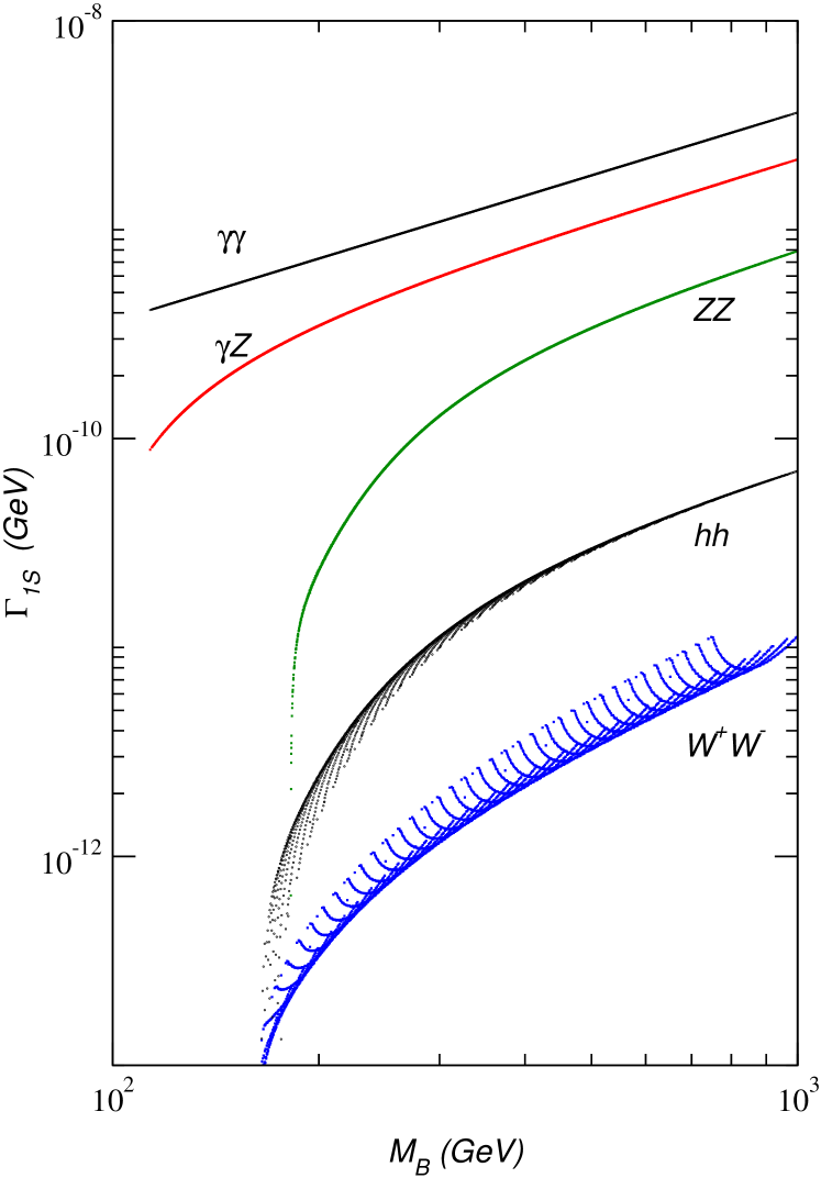
Figure 2: Partial widths of the various decay channels of the $1S$ state, as a function of the bound state mass $M_{B}=2m_{NLSP}$.

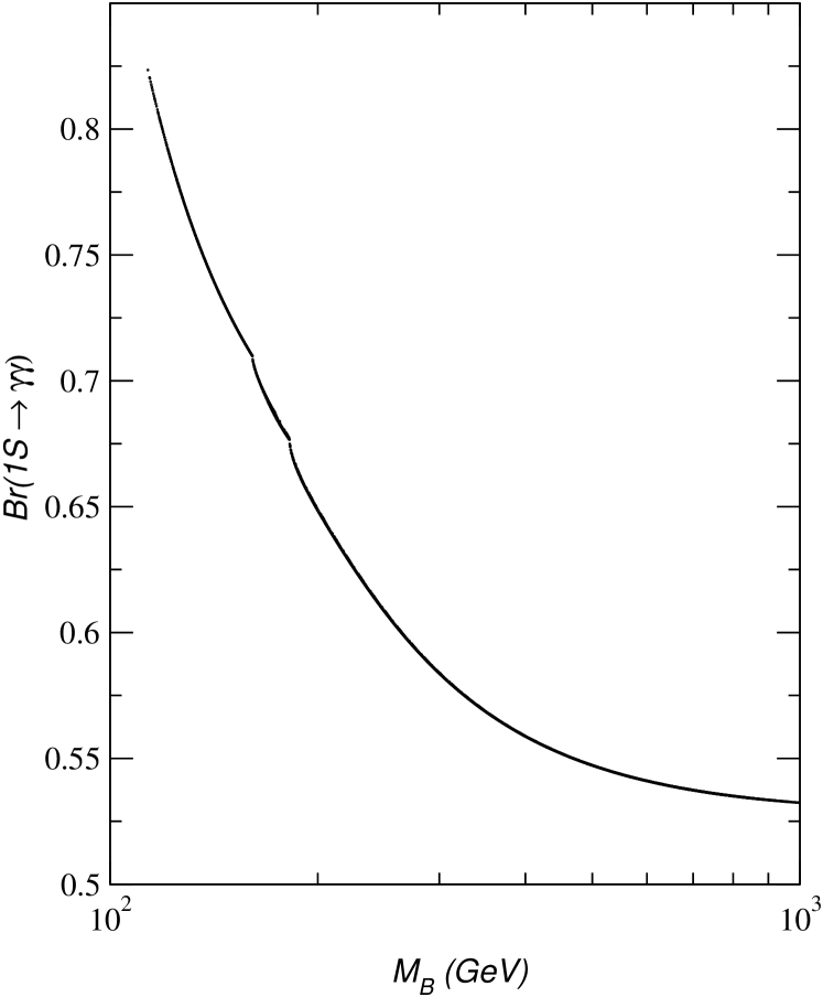
Figure 3: Branching ratio of the $1S\to\gamma\gamma$ decay channel as a function of the bound state mass $M_{B}=2m_{NLSP}$.

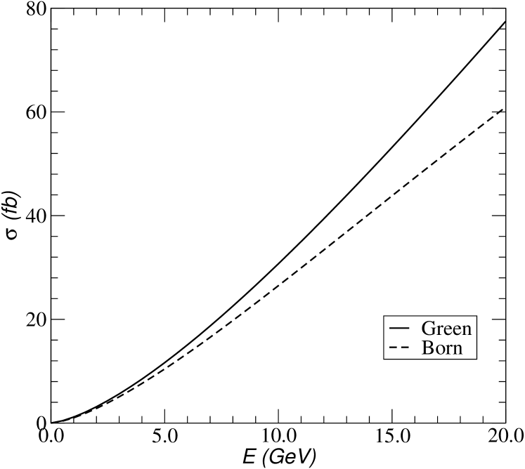
Figure 4: Comparison of the Green function method and the Born level expression for the cross section, for the right smuon. Here we assume that $m_{{\tilde{\mu}}_{R}}=100\textrm{ GeV}$ and a displacement from threshold of up to $20\textrm{ GeV}$.

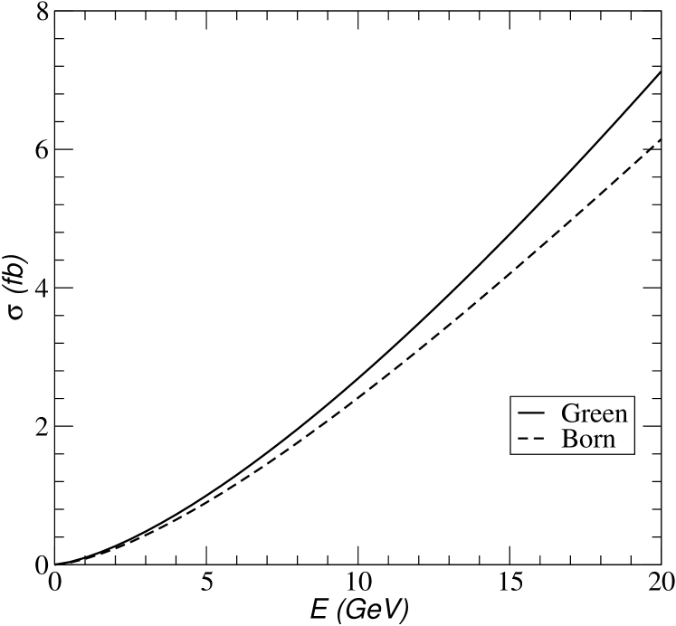
Figure 5: Comparison of the Green function method and the Born level expression for the cross section, for the right smuon. Here we assume that $m_{{\tilde{\mu}}_{R}}=200\textrm{ GeV}$ and a displacement from threshold of up to $20\textrm{ GeV}$.

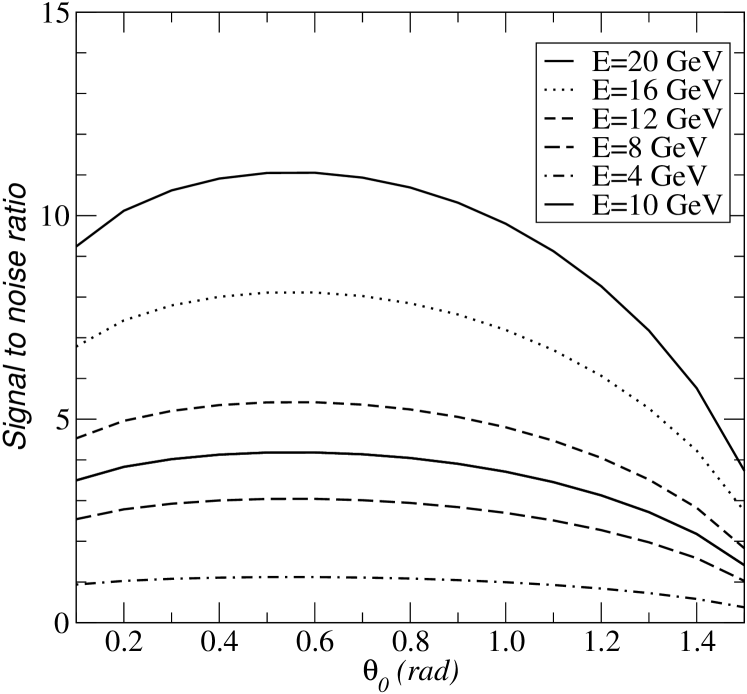
Figure 6: Statistical significance (signal to noise ratio) of the cross section given by the Green function method and the $\gamma\gamma$ QED background as a function of the angular cut angle $\theta_{0}$, for the right smuon $\tilde{\mu}_{R}$. We assume $m_{\tilde{\mu}_{R}}=100$ GeV; the various curves represent different displacements from threshold.

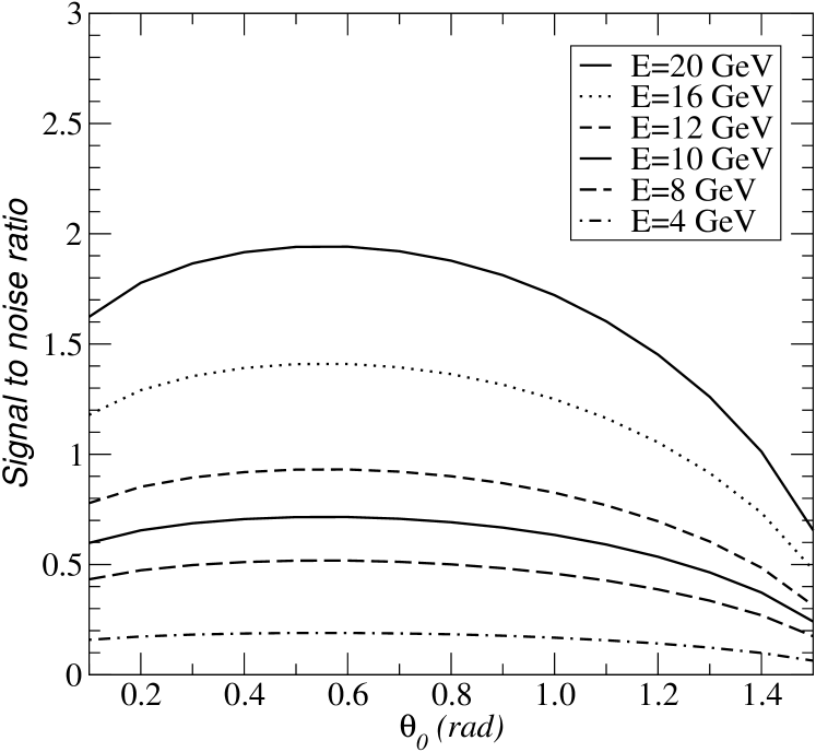
Figure 7: Statistical significance (signal to noise ratio) of the cross section given by the Green function method and the $\gamma\gamma$ QED background as a function of the angular cut angle $\theta_{0}$, for the right smuon $\tilde{\mu}_{R}$. We assume $m_{\tilde{\mu}_{R}}=200$ GeV; the various curves represent different displacements from threshold.

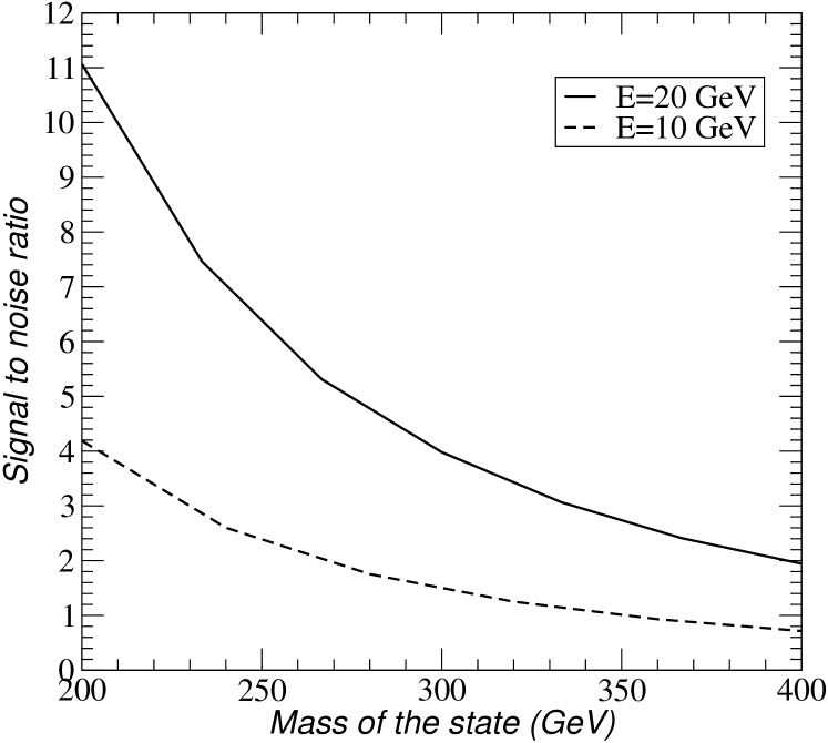
Figure 8: Statistical significance (signal to noise ratio) with respect to the mass of the bound state $M_{B}=2m_{NLSP}$. We show here the case of the right smuon $\tilde{\mu}_{R}$ bound state produced at an energy $E=10$ and $E=20$ GeV above threshold. The angular cut is assumed to be at $\theta_{0}=0.55$, maximal value of the signal to noise ratio.

VII Conclusions

In this work a novel signature at the next LC is proposed for the detection of a sleptonium bound state (of a charged NLSP) assuming that the energy of the collider happens to be around the threshold. It is well known that GMSB models are characterized by large regions of the parameter space in which the NLSP is a charged slepton $\tilde{\ell}_{R}=(\widetilde{e}_{R},\widetilde{\mu}_{R},\widetilde{\tau}_{1})$. While interesting signatures of the production of a pair of charged sleptons NLSP have already been considered in the literature, here we discuss the formation, decay spectroscopy and possible detection of the NLSP (charged slepton) bound state and its possible signature at the next LC. For the sake of simplicity we have considered only the case of $\tilde{\ell}_{R}=\widetilde{\mu}_{R}$.

At an $e^{+}e^{-}$ collider the smuonium bound state is produced in a 2P state. We assume a standard Coulombic interaction to describe the bound states and thereby estimate the energy levels and their separation which are needed to establish whether or not the formation takes place. As a criterion for formation we have chosen the more conservative condition, as opposed to the level gap criterion, obtained by requiring that the revolution time be larger than the lifetime of the rotating constituents. We find out that the formation of the $2P$ bound state is assured for $\sqrt{F_{0}}\geq 14.7\,m_{\tilde{\ell}}$ and thus for all relevant values of $\sqrt{F_{0}}$, the fundamental scale of SUSY breaking. We have first analyzed the decay channels of the $2P$ state. These include: a) decay into a pair of gravitinos, $2P\to\widetilde{G}\widetilde{G}$, b) decay to a pair of standard model fermions $2P\to f\bar{f}$ and c) the dipole transition $2P\to 1S+\gamma$. Studying the partial widths and the branching ratios we find that for all practical purposes the $2P$ state decays to the $1S$ state emitting a photon whose energy is of a few MeV ($\Delta E_{2P-1S}$).

In turn the decay channels of the $1S$ state are to the following final states: $\gamma\gamma,\gamma Z,ZZ,W^{+}W^{-},hh$ and it turns out that the dominant decay is $1S\to\gamma\gamma$ as shown in Figs. 2,3. Thus as the MeV photon from the $2P$ decay goes undetected because its energy is below the detector resolution, the following signal of the sleptonium bound state is defined

$$e^{+}e^{-}\to 2P\to 1S+\text{``soft $\gamma$''}\to\gamma\gamma\,,$$

where the observed final state is two hard back to back photons, and ”practically” no missing energy.

The bound state production cross section has been estimated using the Green function method. Due to the fact that there a bound state actually exists, this effect accounts for a dramatically different cross section with respect to the case of the Born production. For energies just under the threshold, there are several peaks centred at the discrete energy levels of the bound state. Approaching the threshold level from below, those peaks merge and accumulate towards $E=0$ level. This fact translates to the energies above threshold as well ($E>0$), increasing the cross section of the continuum. The net effect is a larger cross section with respect to the naive Born case. This effect grows with the strength of the coupling of the particles which form the bound state itself. It is still very noticeable even for a weak coupling like the sleptonium case, as it is larger than the Born cross section for about 10% to 30%, the difference increasing with the displacement from threshold.

We have given an analysis of the two-photon signal comparing it to the QED two-photon cross-section (at leading order) defining a statistical significance depending on the angular cut which is introduced in order to reduce the QED background. We find that at an energy offset of $E=20$ GeV from the threshold, the statistical significance $SS(\theta_{0})$ (computed for an angular cut $\theta_{0}=0.55$ which maximizes it) goes from $SS=11$ at $m_{\tilde{\ell}_{R}}=100$ with $N_{sig}\approx 5000$ to $SS=2$ for $m_{\tilde{\ell}_{R}}=200$ with $N_{sig}\approx 500$.

Our study has been done assuming a charged slepton co-NLSP scenario which is a peculiarity of GMSB models. On the basis of the results discussed above we conclude that the study of a charged slepton NLSP bound state through the two-photon signature at the next LC has the potential to shed insights into the mechanism of SUSY breaking.

One of the authors (N.F.) wishes do dedicate this work to the memory of Edmondo Pedretti.

References

- (1) H. E. Haber and G. Kane, Phys. Rep. 117 (1985) 75.
- (2) R. Barbieri, Riv. N. Cimento 11 (1988) 1; H. P. Nilles, Phys. Rep. 110 (1984) 1.
- (3) G. F. Giudice and R. Rattazzi, Physics Reports 322 (1999) 419-499.
- (4) L. Randall and R. Sundrum, Nucl. Phys. B557 (1999) 79; G. Giudice, M. Luty, H. Murayama and R. Rattazzi, JHEP 9812 (1998) 027; J. A. Bagger, T. Moroi and E. Poppiz, JHEP 0004 (2000) 009; K. Huitu, J. Laamanen and P. N. Pandita Phys. Rev. D65 (2002) 115003.
- (5) S. Ambrosanio, G. D. Kribs, S. P. Martin, Phys. Rev. D 56 (1997) 1761.
- (6) Stephen P. Martin, E-print arXive: hep-ph/9709356
- (7) S. Dimopulos, G. F. Giudice and A. Pomarol, Phys. Lett. B 389 (1996) 37.
- (8) S. P. Martin Phys. Rev. D. 55 (1997) 3177.
- (9) A. Djouadi, J. L. Kneur and G. Moultaka, Suspect: a Fortran Code for the Supersymmetric and Higgs Particle Spectrum in the MSSM. hep-ph/0211331.
- (10) S. Ambrosanio, B. Mele, S. Petrarca, G. Polesello and A. Imoldi, JHEP01 (2001) 014.
-
(11)
N. Fabiano, A. Grau and G. Pancheri, Phys. Rev. D 50 3173 (1994);
Nuovo Cimento A, Vol. 107, 2789, (1994). - (12) N. Fabiano, Eur. Phys. J. C 2 345 (1998).
- (13) M. Antonelli, N. Fabiano, Eur. Phys. J. C 16 361 (2000).
- (14) G. F. Giudice, M. Mangano, G. Ridolfi, R. Rückl (Convenors) et al, hep-ph/9602207, in G. Altarelli, T. Sjöstrand F. Zwirner (Eds.), Physics at LEP2, Vol. 1, Report CERN 96-01, Geneva 1996.
- (15) M. Peskin and D. Schroeder, An introduction to Quantum Field Theory, Addison & Wesley 1995.
- (16) J. D. Jackson,LBL-5500 Notes for Lectures delivered at SLAC Summer Inst. on Particle Physics, Stanford, Calif., Aug 2-13, 1976
- (17) Manuel Drees and Mihoko M. Nojiri, Phys. Rev D 49, 4595-4615, 1994
- (18) Dimitry S. Gorbunov and Viacheslav A. Ilyin, J. High Energy Phys. JHEP 11 (2000) 011.
- (19) R.Van Royen and V.F.Weisskopf, Nuovo Cimento 50 A (1967) 617, Erratum-ibid.A51:583, (1967).
- (20) Chiara R. Nappi, Physical Review D 25, 84-88, 1982.
- (21) A. S. Davydov, Quantum Mechanics, Second edition, Pergamon Press, Oxford, chapt XII, n.94.
- (22) X. Tata, D.A. Dicus, Phys. Rev. D 35 2110 (1987).
- (23) N. Fabiano, Eur. Phys. J. C 19 547 (2001).
- (24) A.A. Penin, A.A. Pivovarov, Nucl. Phys. B 550 375 (1999).
- (25) Ed. R. Brinkmann, G. Materlik, J. Rossbach, A. Wagner, Conceptual Design of a 500 GeV Linear Collider with Integrated X–Ray Laser Facility, DESY 1997-048, ECFA 1997-182, Vol. 1 (1997).
- (26) TESLA: the superconducting electron positron linear collider with an integrated X-ray laser laboratory. Technical design report. Part. 4: A detector for TESLA. By T. Behnke, (ed.), S. Bertolucci, (ed.), R. D. Heuer, (ed.), R. Settles, (ed.), DESY 2001-011, ECFA 2001-209, Mar 2001. 175pp. Par. 3.2.5
- (27) L. D. Landau and E. M. Lifshitz, Course of Theoretical Physics, Vol. 2, The Classical Theory of Fields, chap. II, 4th revised English edition, Pergamon Press, (1987).