Dark Energy as an Inverse Problem

Abstract

A model–independent approach to dark energy is here developed by considering the determination of its equation of state as an inverse problem. The reconstruction of $w(z)$ as a non–parametric function using the current SNe Ia data is explored. It is investigated as well how results would improve when considering other samples of cosmic distance indicators at higher redshift. This approach reveals the lack of information in the present samples to conclude on the behavior of $w(z)$ at z $>$ 0.6. At low level of significance a preference is found for $w_{0}$ $<$ –1 and $w^{\prime}(z)$ $>$ 0 at z $\sim$ 0.2–0.3. The solution of $w(z)$ along redshift never departs more than 1.95 $\sigma$ from the cosmological constant $w(z)=-1$, and this only occurs when using various cosmic distance indicators. The determination of $w(z)$ as a function is readdressed considering samples of large number of SNe Ia as those to be provided by SNAP. It is found an improvement in the resolution of $w(z)$ when using those synthetic samples, which is favored by adding data at very high z. The set of degenerate solutions compatible with the data can be retrieved through this method.

I Introduction

The acceleration of the rate of expansion of the Universe, first discovered through supernovae Riess et al. (1998); Perlmutter et al. (1999) is being confirmed by new cosmological tests. The cosmic microwave background measurements by the Wilkinson Microwave Anisotropic Probe (WMAP) Spergel et al. (2003) and results from the large scale distribution of galaxies Percival et al. (2001) and galaxy clusters Allen et al. (2003) confirm that our universe is dominated by negative pressure. The understanding of the accelerated expansion of the cosmos might result in a change of the framework in which gravity is to be described or in the identification of unknown components of the cosmos. All this seems most fundamental to physics and cosmology, thus large samples of cosmological data and various procedures to analyse them are being examined.

In a descriptive way, the component or new physics responsible for the acceleration of the expansion, the so called “dark energy”, can be incorporated in the right–hand side of the Friedmann–Robertson–Walker (FRW) equations and be simply addressed as an additional term for whom we intend to determine the barotropic index: $w(z)=p(z)/\rho(z)$.

The reconstruction of $w(z)$ from a given sample of data has been attempted proposing fitting functions or expansion series of $w(z)$ along z in ways to accomodate a wide range of dark energy candidates Saini et al. (1999); Gerke & Efstathiou (2002); Linder (2003); Daly & Djorgovski (2004); Visser (2004); Nesseris & Perivolaropoulos (2004); Huterer & Starkman (2003); Huterer & Cooray (2004); Alam et al. (2003, 2004); Jonsson et al. (2004); Bassett al. (2002); Parkinson al. (2004); Bassett al. (2004); Feng al. (2005). There has been some debate on the effect that choosing particular models for those functions or truncating the expansion series in z might have in deriving possible evolution Jonsson et al. (2004); Linder (2002); Alam et al. (2003, 2004, 2004).

Here, we have developed an approach to obtain $w(z)$ without imposing any constraints on the form of the function. This is addressed through a generalized nonlinear inverse approach. This method allows to examine the resolution of the equation of state $w(z)$ at various redshifts and through various samples. One can quantify the improvement in information provided by increasing a sample or by the addition of various sources. The inverse approach formulated by Backus and Gilbert(1970)Backus & Gilbert (1970) has been widely used in geophysics and solar structure physics. In this approach, the mere fact that the continuous functional has to be derived from a discrete number of data implies a non–uniqueness of the answer. It has also been shown that, even if the data were dense and with no uncertainty, there would be more than one solution to many specific inverse problems such as the determination of the density structure of the earth from the data on the local gravitational field at its surface, and others. This lack of uniqueness comes from the way in which the different equations reflect in the observables used. The problem of the determination of dark energy faces such degeneracy. In the luminosity distance along z from supernovae and other cosmic distance indicators, $w(z)$ enters in an integral form, which limits the possibility to access to $w(z)$.

In earlier examinations of the degeneracy in $w(z)$ obtained through cosmic distance indicators a range of solutions giving the same luminosity distance along z were pointed out Maor et al. (2001); Maor & Brustein (2003). As more data would constrain $w(z)$ at various redshifts, not only using the distance luminosity, but other indicators as well, the reconstruction should become more successful.

To compare with a significant body of work which analyses the data using the expansion to first order $w(z)=w_{0}+w_{a}z/(1+z)$, we will also formulate this approach for the case of determination of discrete parameters. This allows to quantify the increase of information among SNe Ia samples and samples of other distance indicators. We examine from current data the possibility of determining at present the values of $w(z)$ and its first derivative and compare with previous results Jonsson et al. (2004); Riess et al. (2004).

II Inverse problem

II.1 Non–parametric non–linear inversion

The inverse problem provides a powerful way to determine the values of functional forms from a set of observables. This approach is useful when the information along a certain coordinate, in our case information on $w(z)$, emerges in observables coupled with information at all other z. We have a surface picture of $w(z)$ in the luminosity distance at a given z, as the p–mode waves in the Sun surface have on its internal structure. Dark energy is here addressed using the non–linear non–parametric inversion. Most frequently, when the parameters to be determined are a set of discrete unknowns, the method used is a least squares. But the continuos case, where functional forms are to be determined, requires a general inverse problem formulation. The inverse method used here is a Bayesian approach to this generalization Tarantola & Valette (1982).

We consider a flat universe with only two dominant constituents (at present): cold matter and dark energy. Therefore we characterize the cosmological model by the density of matter, $\Omega_{M}$, and by the index $w(z)$ of the dark energy equation of state,

$$w(z)=\frac{p(z)}{\rho(z)}$$ (1)

The vector of unknowns M has then a discrete and a continuous component,

$$\textrm{{M}}=\left(\begin{array}[]{c}\Omega_{M}\\ w(z)\\ \end{array}\right)\$$ (2)

On the other hand, the observational data are mainly SNe Ia magnitudes. We have a finite set of $N$ magnitudes, $m_{i}$, and consider the following theoretical equation, the magnitude-redshift relation in a flat universe relating the unknowns to the observational data:

$$m^{th}(z,\Omega_{M},w(z))={\cal M}~{}+5\log[D_{L}(z,\Omega_{M},w(z))],$$ (3)

where

$${\cal M}\equiv M-5\log H_{0}+25$$ (4)

and $D_{L}$ is the Hubble-free luminosity distance

$$D_{L}(z,\Omega_{M},w(z))=c(1+z)\int_{0}^{z}{\frac{H_{0}dz^{\prime}}{H(z^{\prime},\Omega_{M},w(z))}}$$ (5)

with

$$H(z^{\prime},\Omega_{M},w(z))=H_{0}~{}\sqrt{\Omega_{M}(1+z^{\prime})^{3}+\Omega_{X}(z^{\prime})}$$ (6)

$$\Omega_{X}(z)=\Omega_{X}\exp{\left(3\int_{0}^{z}{dz^{\prime}\frac{1+w(z^{\prime})}{1+z^{\prime}}}\right)}.$$ (7)

In order to combine the results with other data we substitute the original SNe magnitudes by the dimensionless distance coordinate $y$:

$$y_{i}\equiv\frac{exp_{10}{((m_{i}-{\cal M})/5)}}{c(1+z_{i})}=\int_{0}^{z_{i}}{\frac{dz^{\prime}}{\sqrt{\Omega_{M}(1+z^{\prime})^{3}+\Omega_{X}(z^{\prime})}}},$$ (8)

$$\sigma_{y_{i}}=\frac{\ln 10}{5}y_{i}(\sigma_{m_{i}}+\sigma_{\cal M}).$$ (9)

With this definition we deal directly with a function $y(\Omega_{M},w(z))$, the only part which depends on the cosmological model. To convert our $m_{i}$ data to $y_{i}$, we can adopt the value obtained from low redshift supernovae and use ${\cal M}=-3.40\pm 0.05$. Defined in this way, $y_{i}$ is used in other analyses Daly & Djorgovski (2004).

After the corresponding transformations, the observables are now described by a vector of $N$ components, $y_{i}$, and by a covariance matrix ($\textrm{{C}}_{y}$). This method can handle correlated measurements, where non–diagonal elements $C_{y_{i}y_{j}}$ are different from zero (observations i and j being correlated). But, at present, those have not been estimated for the composite samples of distance indicators. We would then use:

$$C_{y,ij}=\sigma^{2}_{y_{ij}}\delta_{ij}$$ (10)

The unknown vector of parameters is described by its a priori value, $\textrm{{M}}_{0}$, and the covariance matrix ($\textrm{{C}}_{0}$). The function describing $w(z)$ should be smooth. This leads to no null covariance between neighboring points in z for $w(z)$ (the smoothness of $w(z)$ implies that if at z, the value of $w(z)$ has a deviation $w(z)-w(z^{\prime})$ of a given sign and magnitude, we want, at a neighboring point z^′, the deviation $w(z)-w(z^{\prime})$ to have a similar sign and magnitude.

Thus, the covariance matrix $\textrm{{C}}_{0}$ has the form:

$$\textrm{{C}}_{0}=\left(\begin{array}[]{cc}\sigma^{2}_{\Omega_{M}}&0\\ 0&C_{w(z),w(z^{\prime})}\\ \end{array}\right)$$ (11)

where a choice is made for the non–null covariance between z and z^′, $C_{w(z),w(z^{\prime})}$. This choice is taken to be as general as possible. It would define the smoothness required in the solution by setting the correlation length between errors in z and z^′ (this gives the length scale in which the function can fluctuate between redshifts). The amplitude of the fluctuation of the function is given by the dispersion $\sigma_{w}$ at z. In the Gaussian choice for $C_{w(z),w(z^{\prime})}$, $\sigma_{w}$ is the 1$\sigma$ region where the solution is to be found.

Thus for a Gaussian choice, $C_{w(z),w(z^{\prime})}$ is described as:

$$C_{w(z),w(z^{\prime})}=\sigma_{w}^{2}\exp\left(-\frac{(z-z^{\prime})^{2}}{2\Delta_{z}^{2}}\right),$$ (12)

which means that the variance at z equals $\sigma_{w}^{2}$ and that the correlation length between errors is $\Delta_{z}$. Another possible choice for $C_{w(z),w(z^{\prime})}$ is an exponential of the type:

$$C_{w(z),w(z^{\prime})}=\sigma_{w}^{2}\exp\left(-\frac{|z-z^{\prime}|}{\Delta_{z}}\right),$$ (13)

while no difference in the results is found by those different choices of $C_{w(z),w(z^{\prime})}$.

We are interested in determining the best estimator ${\tilde{\textrm{{M}}}}$ for M. The probabilistic approach incorporates constraints from priors through the Bayes theorem, i.e, the a posteriori probability density $f_{post}(\textrm{{M}}/\textrm{{D}})$ for the vector M containing the unknown model parameters given the observed data D, is linked to the likelihood function L and the prior density function for the parameter vector as:

$$f_{post}(\textrm{{M}}/\textrm{{D}})\,\,\alpha\,{\it L}(\textrm{{D}}/\textrm{{M}})\,\,\cdot\,f_{prior}(\textrm{{M}})$$ (14)

The theoretical model described by the operator $\textrm{{y}}^{th}$, which connects the model parameters M with the predicted data $\textrm{{D}}_{predicted}=\textrm{{y}}^{th}(\textrm{{M}})$ is to agree as closely as possible with the observed data y. Assuming that both the prior probability and the errors in the data are distributed as Gaussian functions, the posterior distribution becomes:

$$f_{post}(\textrm{{M}}/\textrm{{y}})\,\alpha\,exp[-\frac{1}{2}~{}(\textrm{{y}}-\textrm{{y}}^{th}(\textrm{{M}}))^{*}~{}\textrm{{C}}_{y}^{-1}~{}(\textrm{{y}}-\textrm{{y}}^{th}(\textrm{{M}}))$$

$$-\frac{1}{2}~{}(\textrm{{M}}-\textrm{{M}}_{0})^{*}~{}\textrm{{C}}_{0}^{-1}~{}(\textrm{{M}}-\textrm{{M}}_{0})]$$

(15)

where ^∗ stands for the adjoint operator. The best estimator for M, $\tilde{\textrm{{M}}}$, is the most probable value of M, given the set of data y. The condition is reached by minimizing the misfit function:

$$S\equiv\frac{1}{2}~{}(\textrm{{y}}-\textrm{{y}}^{th}(\textrm{{M}}))^{*}~{}\textrm{{C}}_{y}^{-1}~{}(\textrm{{y}}-\textrm{{y}}^{th}(\textrm{{M}}))+$$

$$\frac{1}{2}~{}(\textrm{{M}}-\textrm{{M}}_{0})^{*}~{}\textrm{{C}}_{0}^{-1}~{}(\textrm{{M}}-\textrm{{M}}_{0}),$$ (16)

which is equivalent to maximize the Gaussian density of probability when data and parameters are treated in the same way. This Bayesian approach helps to regularize the inversion.

Let us now define the operator G represented by the matrix of partial derivatives of the dimensionless distance coordinate, which will simplify subsequent notation. Its kernel will be denoted by $g$.

$$\textrm{{G}}=\left(\begin{array}[]{cc}\frac{\partial y_{1}^{th}}{\partial\Omega_{M}}&\frac{\partial y_{1}^{th}}{\partial w(z)}\\ \frac{\partial y_{2}^{th}}{\partial\Omega_{M}}&\frac{\partial y_{2}^{th}}{\partial w(z)}\\ :&:\\ \frac{\partial y_{N}^{th}}{\partial\Omega_{M}}&\frac{\partial y_{N}^{th}}{\partial w(z)}\end{array}\right)$$ (17)

with

$$\frac{\partial y_{i}^{th}}{\partial\Omega_{M}} = -\frac{1}{2}\int_{0}^{z_{i}}\frac{(1+z^{\prime})^{3}dz^{\prime}}{H^{3}(z^{\prime})}$$ (18)

$$\equiv \int_{0}^{z_{i}}g_{\Omega_{M}}(z^{\prime})dz^{\prime},$$

$$\frac{\partial y_{i}^{th}}{\partial w(z)} = -\frac{1}{2}\int_{0}^{z_{i}}\frac{3\Omega_{X}(z^{\prime})\ln(1+z^{\prime})dz^{\prime}}{H^{3}(z^{\prime})}$$ (19)

$$\equiv \int_{0}^{z_{i}}g_{w}(z^{\prime})dz^{\prime}.$$

As shown in Eq. 3 or equivalently Eq. 8, the inverse problem is nonlinear in the parameters, thus the solution is reached iteratively in a gradient based search. To minimize $S$ in Eq. 16, one demands stationarity. For the non–linear case the solution has to be implemented as an iterative procedure where Tarantola & Valette (1982):

$$\tilde{\textrm{{M}}}_{[k+1]}=\textrm{{M}}_{0}~{}+~{}\textrm{{C}}_{0}~{}\textrm{{G}}^{*}_{[k]}~{}(\textrm{{C}}_{y}+\textrm{{G}}_{[k]}\textrm{{C}}_{0}~{}\textrm{{G}}^{*}_{[k]})^{-1}$$

$$(\,\textrm{{y}}~{}-~{}\textrm{{y}}^{th}(\tilde{\textrm{{M}}}_{[k]})~{}+~{}\textrm{{G}}_{[k]}~{}(\tilde{\textrm{{M}}}_{[k]}-\textrm{{M}}_{0})\,)$$ (20)

The estimate of the dimensionless distance coordinates in the iterations is given by:

$$\tilde{\textrm{{y}}}_{[k+1]}=\textrm{{y}}~{}-~{}\textrm{{C}}_{y}~{}(\textrm{{C}}_{y}+\textrm{{G}}_{[k]}\textrm{{C}}_{0}~{}\textrm{{G}}^{*}_{[k]})^{-1}$$

$$(\,\textrm{{y}}~{}-~{}\textrm{{y}}^{th}(\tilde{\textrm{{M}}}_{[k]})~{}+~{}\textrm{{G}}_{[k]}~{}(\tilde{\textrm{{M}}}_{[k]}-\textrm{{M}}_{0})\,)$$ (21)

Since we are working in a Hilbert space with vectors containing functional forms, the above operator products give rise to scalar products of the functions integrated over the domain of those functions. The expressions transform into having the above products rewritten in terms of the kernels of the operators Tarantola & Nercessian (1984).

We will indicate the scalar product by “ $\cdot$ ” and it is defined as it can be seen from this example:

$$C_{w}\cdot\frac{\partial y_{j}^{th}}{\partial w(z)}=\int_{0}^{z_{j}}dz^{\prime}C_{w}(z,z^{\prime})g_{w}(z^{\prime}),$$ (22)

The components of the vector of unknowns $\tilde{\textrm{{M}}}$, which in our case will be both $\Omega_{M}$ and $w(z)$, are then obtained from:

$$\tilde{M}_{[k+1]}(z)=M_{0}(z)+$$

$$\sum_{i=1}^{N}W_{i[k]}\int_{0}^{z_{i}}C_{0}(z,z^{\prime})g_{i[k]}(z^{\prime})dz^{\prime}$$ (23)

where

$$W_{i[k]}=\sum_{j=1}^{N}\left(S_{[k]}^{-1}\right)_{i,j}V_{j[k]}$$ (24)

V $$= \textrm{{y}}+~{}\textrm{{G}}~{}(\textrm{{M}}-\textrm{{M}}_{0})-\textrm{{y}}^{th}(\textrm{{M}})$$

$$V_{i[k]} = y_{i}+\int_{0}^{z_{i}}g_{j[k]}(z)\left(M_{[k]}(z)-M_{0}(z)\right)dz$$ (25)

$$-\,y_{i}^{th}(z_{i},\Omega_{M},w(z))$$

S $$= \textrm{{C}}_{y}~{}+~{}\textrm{{G}}~{}\textrm{{C}}_{0}~{}\textrm{{G}}^{*}$$

$$S_{i,j[k]} = (C_{y})_{i,j}+$$

$$\int_{0}^{z_{j}}\int_{0}^{z_{i}}g_{i[k]}(z)\,C_{0}(z,z^{\prime})\,g_{j[k]}(z^{\prime})\,dz\,dz^{\prime}$$

In the case of the dark energy equation of state and the matter density the expressions reduce to

$$\Omega_{M[k+1]}=\Omega_{Mo}+\sigma_{\Omega_{M}}^{2}\sum_{i=1}^{N}W_{i\,[k]}\,{\frac{\partial y_{i}^{th}}{\partial\Omega_{M}}}_{[k]}$$ (27)

$$w_{[k+1]}(z)=w_{o}(z)+\sum_{i=1}^{N}W_{i\,[k]}\int_{0}^{z_{i}}C_{w}(z,z^{\prime})g_{w}(z^{\prime})_{[k]}dz^{\prime}$$ (28)

where $C_{w}(z,z^{\prime})\equiv C_{w(z),w(z^{\prime})}(z,z^{\prime})$, $W_{i\,[k]}$ is given by the product (24) with:

$$V_{i} = y_{i}+\frac{\partial y_{i}^{th}}{\partial\Omega_{M}}(\Omega_{M}-\Omega_{M_{0}})+\frac{\partial y_{i}^{th}}{\partial w(z)}\cdot(w-w_{o})$$ (29)

$$-\,y_{i}^{th}(z_{i},\Omega_{M},w(z))$$

$$S_{i,j} = \delta_{i,j}\sigma_{i}\sigma_{j}+\frac{\partial y_{i}^{th}}{\partial\Omega_{M}}C_{\Omega_{M}}\frac{\partial y_{j}^{th}}{\partial\Omega_{M}}+$$ (30)

$$\frac{\partial y_{i}^{th}}{\partial w(z)}\cdot\left(C_{w}\cdot\frac{\partial y_{j}^{th}}{\partial w(z)}\right)$$

To test the accuracy of the inversion we use the a posteriori covariance matrix. It can be shown (see Tarantola & Valette (1982b); Tarantola & Nercessian (1984)) that for the linear inverse problem with Gaussian a priori probability density function, the a posteriori probability density function is also Gaussian with mean Eq. II.1 and covariance Eq. 31. Although its value is only exact in the linear case it is a good approximation here, since the luminosity distance is quite linear on the equation of state $w(z)$ at low redshift.

$$\textrm{{C}}_{\tilde{\rm{M}}} = (\,\textrm{{G}}^{*}\,\textrm{{C}}_{y}^{-1}\,\textrm{{G}}\,+\,\textrm{{C}}_{0}^{-1}\,)^{-1}\equiv\textrm{{C}}_{0}-\textrm{{C}}_{0}\,\textrm{{G}}^{*}\,\textrm{{S}}^{-1}\,\textrm{{G}}\,\textrm{{C}}_{0}$$ (31)

$$= (\,\textrm{{I}}-\textrm{{C}}_{0}\,\textrm{{G}}^{*}\,\textrm{{S}}^{-1}\,\textrm{{G}}\,)\,\textrm{{C}}_{0}$$

In an explicit form, the standard deviations from this covariance read

$$\tilde{\sigma}_{\Omega_{M}} = \sqrt{C_{\tilde{\Omega}_{M}}}=$$

$$= \sigma_{\Omega_{M}}\sqrt{1-\sum_{i,j}\frac{\partial y_{i}^{th}}{\partial\Omega_{M}}(S^{-1})_{i,j}\frac{\partial y_{j}^{th}}{\partial\Omega_{M}}\sigma_{\Omega_{M}}^{2}}$$

$$\tilde{\sigma}_{w(z)}(z) = \sqrt{C_{\tilde{w}(z)}(z)}=$$

$$= \sqrt{\sigma_{w(z)}^{2}-\sum_{i,j}C_{w}\cdot\frac{\partial y_{i}^{th}}{\partial w(z)}(S^{-1})_{i,j}\frac{\partial y_{j}^{th}}{\partial w(z)}\cdot C_{w}}$$

where the symbols with tilde are the a posteriori values, whereas the symbols without represent the a priori ones.

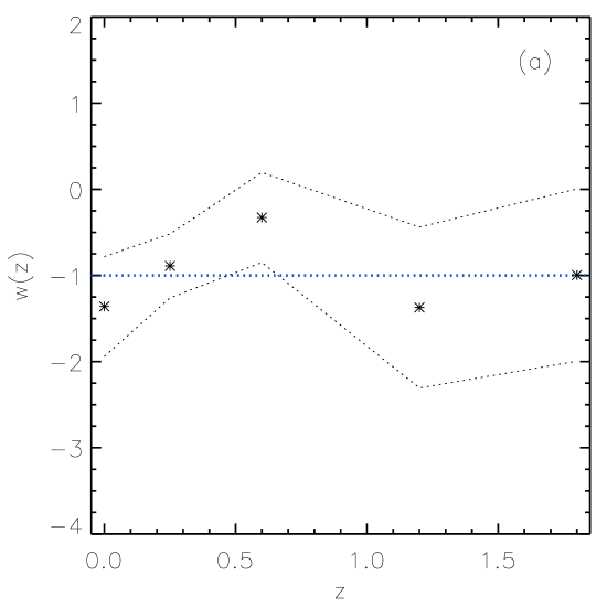
Figure 1: Reconstruction of $w(z)$ using the 156 SNe from the gold set of Riess et al.(2004) Riess et al. (2004). $C_{w(z),w(z^{\prime})}$ is Gaussian with $\sigma_{w}=1$ and correlation length $\Delta_{z}=0.08$. At high z, the lack of enough data does not allow to improve the initial knowledge, as seen in $\tilde{\sigma}_{w(z)}(z)=\sqrt{C_{\tilde{w}(z)}(z)}$. Low–resolution inversions (as exemplified here with $\delta z=$0.3 at low z, and $\delta z=$ 0.6 at high z) and high resolution ones (as with $\delta z=$0.06 in Figure 2) give consistent results.

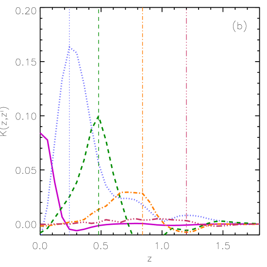
Figure 2: Reconstruction of $w(z)$ with 156 SNe from the gold set of Riess et al. (2004). These results are obtained using Gaussian a priori covariances with amplitude $\sigma_{w}=0.5$ and $\Delta_{z}=0.08$. This fine grid calculation uses $\delta$z $=$ 0.06. The upper panel shows $w(z)$ (solid line) and the $1\sigma$ confidence interval (dashed shadow). Below, the different resolving kernels at z $=0,0.24,0.48,0.84,1.20$ are shown. The resolving kernels at high z show that there is no information to conclude on the evolution of the equation of state at z$>$0.6.

There are other parameters which help to interpret the results. From the form of Eq. 31 we see that the operator $\textrm{{C}}_{0}\textrm{{G}}^{*}\textrm{{S}}^{-1}\textrm{{G}}$ is related to the obtained resolution. This is usually called the resolving kernel $K(z,z^{\prime})$. The more this term resembles the $\delta$-function the smaller the a posteriori covariance function is. In fact, in the linear case, the resolving kernel represents how much the results of the inversion differ from the true model. It equals to be the filter between the true model and its estimated value Backus & Gilbert (1970); Tarantola & Valette (1982). In any applied case, it is a low band pass filter which depends on the data available and the details requested from the model.

It can also be expressed in terms of the a priori and the a posteriori covariance matrices:

$$\textrm{{K}}\,=\,\textrm{{I}}\,-\,\textrm{{C}}_{\tilde{\rm{M}}}~{}\textrm{{C}}_{0}^{-1}$$ (34)

This expression will be evaluated numerically to quantify the resolution and information generated in the inversion. Another term of interest is the mean index, which is derived from the resolving kernel:

$$I(z)=\int K(z,z^{\prime})dz^{\prime}.$$ (35)

The nearest $I(z)$ to $1$, the most restrictive are the data to the model. For very low values, data do not improve our prior knowledge on the parameters.

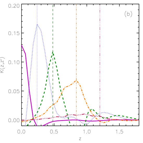
Figure 3: Reconstruction of $w(z)$ (as in Figure 2) but with the 156 SNe from the gold set of Riess et al. (2004) and 20 RG from Daly & Djorgovski (2004).

II.2 Discrete parameters

In the previous section we have obtained the results for a set of a continuous function and a discrete parameter, but we can also consider the case of various discrete parameters. It was pointed out that a succesful parametrization for modeling a large variety of dark energy models is obtained by considering $w(z)$ expanded around the scale factor $a$. The earlier parametrization to first order in z given by $w(z)=w_{0}+w^{\prime}z$ proved unphysical for the CMB data and a poor approach to SN data at z $\sim$ 1 Linder (2002). For the case of moderate evolution in the equation of state, the most simple (two–parameter) description of $w(z)$ so far proposed is (2001); Linder (2003):

$$w(z)=w_{0}+w_{a}(1-a)$$ (36)

where the scale factor $a=(1+z)^{-1}$ and $w(z)$ turns out:

$$w(z)=w_{0}+w_{a}\frac{z}{1+z}.$$ (37)

We use now this particular form for the function $w(z)$ commonly used to study the behaviour of dark energy to solve iteratively for $w_{0}$ and $w_{a}$:

$$w_{0[k+1]}=w_{0}^{0}+\sigma_{w_{0}}^{2}\sum_{i=1}^{N}W_{i\,[k]}\frac{\partial y_{i}^{th}}{\partial w_{0}}_{[k]}$$ (38)

$$w_{a[k+1]}=w_{a}^{0}+\sigma_{w_{a}}^{2}\sum_{i=1}^{N}W_{i\,[k]}{\frac{\partial y_{i}^{th}}{\partial w_{a}}}_{[k]}$$ (39)

where

$$\frac{\partial y_{i}^{th}}{\partial w_{0}}=-\frac{1}{2}\int_{0}^{z_{i}}\frac{3\Omega_{X}(z^{\prime})\ln(1+z^{\prime})dz^{\prime}}{H^{3}(z^{\prime})},$$ (40)

$$\frac{\partial y_{i}^{th}}{\partial w_{a}}=-\frac{1}{2}\int_{0}^{z_{i}}\frac{3\Omega_{X}(z^{\prime})[\ln(1+z^{\prime})-\frac{z^{\prime}}{1+z^{\prime}}]dz^{\prime}}{H^{3}(z^{\prime})}.$$ (41)

The a posteriori variance is for these parameters:

$$\tilde{\sigma}_{w_{0}}=\sqrt{C_{\tilde{w}_{0}}}=\sigma_{w_{0}}\sqrt{1-\sum_{i,j}\frac{\partial y_{i}^{th}}{\partial w_{0}}(S^{-1})_{i,j}\frac{\partial y_{j}^{th}}{\partial w_{0}}\sigma_{w_{0}}^{2}}$$ (42)

$$\tilde{\sigma}_{w_{a}}=\sqrt{C_{\tilde{w}_{a}}}=\sigma_{w_{a}}\sqrt{1-\sum_{i,j}\frac{\partial y_{i}^{th}}{\partial w_{a}}(S^{-1})_{i,j}\frac{\partial y_{j}^{th}}{\partial w_{a}}\sigma_{w_{a}}^{2}}$$ (43)

The equations for $\Omega_{M}$ are those of section II (Eqs. 27,  18 and  II.1).

III Present and Future Samples

We briefly introduce the various samples used here for the exploration of dark energy and for measuring the increase of information in $w(z)$ along the last years. An initial sample of SNeIa at high z was presented in 1999 by the SCP (Supernova Cosmology Project)Perlmutter et al. (1999). The set includes 16 low-redshift supernovae from the Calán/Tololo survey and 38 high-redshift supernovae Perlmutter et al. (1999). The new data of this collaboration (low-extinction primary subset in Knop et al. (2003)) adds 11 high redshift SNe Ia observed with the Hubble Space Telescope (HST). The third SNIa set examined corresponds to the gold set buildt up with 7 SNeIa at z $>$ 1 by GOODS and a combination of different previous samples revised to follow the same calibrations Riess et al. (2004). With this last set it has been doubled the maximum redshift and triplicated the number of data as compared with the first one.

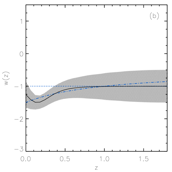
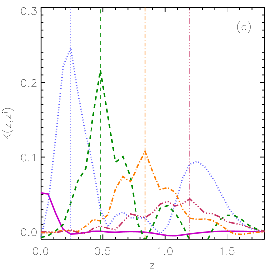
Figure 4: Results with 2000 SNe from SNAP plus 300 SNe from SNF. Gaussian covariance is as in Figure 2 an 3. In the upper panel it is shown the deviation in luminosity distance between model and the cosmological constant i.e. $(d_{L}^{m}-d_{L}^{\Lambda})/d_{L}^{\Lambda}$. The recovered $w(z)$ is shown in the middle panel and the resolving kernels in the low panel. The reconstruction, (shown in solid line in the middle panel) clearly points out that at intermediate redshift the best model is not the cosmological constant (dotted line), which served as prior. The inversion recovers the shape of the true dark energy model $w(z)$. The dot–dashed line starting at w(0)$=$ –1.5 is the fiducial dark energy model with $w(z)=-1.5+1.0z/(1+z)$. The same result is found with a wider prior. The fiducial model at z$=$ 0 is below $(d_{L}^{m}-d_{L}^{\Lambda})/d_{L}^{\Lambda}$ $=$ 1 $\%$ and away of the prior at z=0, but this does not preclude to obtain the slope of the function.

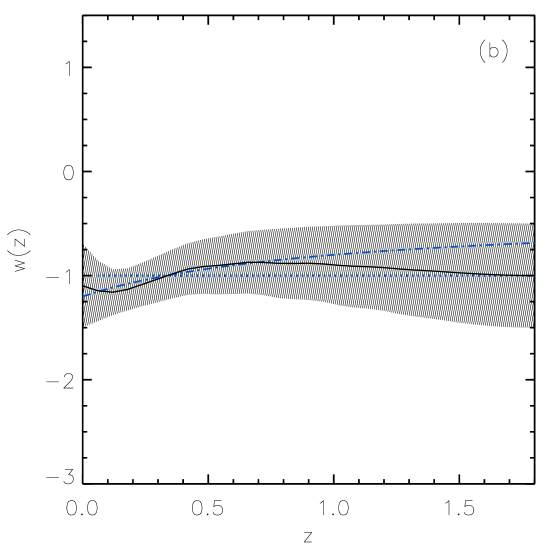
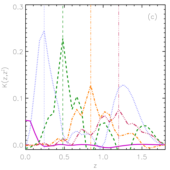
Figure 5: Reconstruction of $w(z)$ (as Figure 4), but now the fiducial model (dot–dashed line) is $w(z)=-1.2+0.8z/(1+z)$ and is closer in luminosity distance to the prior (dotted line), taken to be the cosmological constant. In the upper panel it is shown the deviation in luminosity distance between models, i.e. $(d_{L}^{m}-d_{L}^{\Lambda})/d_{L}^{\Lambda}$. The true model is recovered at redshifts where the deviation is more than $1\%$ (a relative difference of 1% in distance luminosity corresponds to a magnitude difference between models of $\sim$ 0.02 mag, which at high z is the limiting factor to differentiate between models). This inversion finds the best solution for models which depart at intermediate z from the cosmological model at more than 1$\%$ in $d_{L}$. This result is independent of the width of the prior.

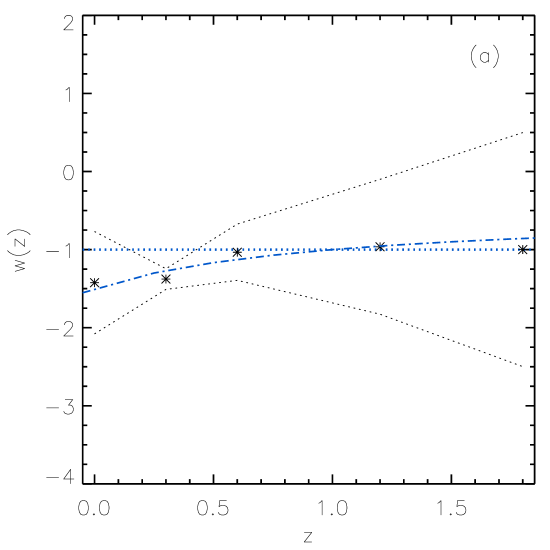
Figure 6: Low resolution reconstruction (5 points calculated as in Figure 1) of $w(z)$ with the SNAP data set simulated and the fiducial model with $w(z)=-1.5+1.0z/(1+z)$. It is shown how this model would be differentiated from the cosmological constant at more than 2$\sigma$ at intermediate z, in agreement with what is discussed in Figure 4. These results are obtained using much wider Gaussian a priori covariances than in the high resolution case ($\sigma_{w}=2.0$).

The SNIa samples available at present are still small, and, therefore, we also use synthetic samples resembling those to be acquired by the Supernova Acceleration Probe (SNAP) http://snap.lbl.gov/ . To generate these samples we assume the redshift distribution of 2000 SNeIa from Kim et al. (2001). For every supernova we calculate its magnitude given a fiducial dark energy model. Our first model corresponds to the cosmological constant in a universe with density parameters $\Omega_{M}=0.3$ and $\Omega_{\Lambda}=0.7$ (this model has $w_{0}=-1$ and $w_{a}=0$). We generate other synthetic samples based on dark energy models inspired in supergravity theories Weller & Albrecht (2001)) with $\Omega_{M}=0.3$, $w_{0}$ negative and positive $w_{a}$. Various values of $w_{0}$ and $w_{a}$ are tried ($w_{0}$ range from –1.5 to –0.8 and $w_{a}$ range from 0.6 to 1). Gaussian errors are added to the supernova data, taking into account the statistical error per supernova after the corresponding calibrations ($\sigma_{st}=~{}0.15$). The level of residual systematic error corresponds to the design of SNAP Kim et al. (2001), which should achieve 0.02 mag systematic error in redshifts bins of width $\Delta z$ $=$ 0.1 with a dependence in z, $\sigma_{sys}=0.02~{}z/z_{max}$ Kim et al. (2001).

The error of the measurement in each z bin, is given by:

$$\sigma_{bin}=\sqrt{\frac{\sum\sigma_{st}^{2}}{N_{bin}}+\sigma_{sys}^{2}}$$ (44)

where $N_{bin}$ is the number of supernovae in each bin. To this distribution we also add 300 nearby SNe, as those expected from the Nearby Supernova Factory http://snfactory.lbl.gov/ . A total amount of 2300 SNeIa are used. As discussed in Frieman et al. (2001), with a large data set, the irreducible systematic error is putting the limit to our possibilities of recovering the dark energy equation of state.

At the moment, the low numbers of SNe Ia found at z$>$ 1, impact in the reconstruction of the equation of state. Although SNe Ia are the best known calibrated candles at high redshift, we can explore other luminous sources that could be reliable distance indicators to study dark energy. Among these, the Fanaroff–Riley type IIb radio galaxies (FR IIb) are a group of galaxies quite homogeneous along redshift Daly & Guerra (2002). Their angular size measured from the outer edges of their lobes can be used to determine angular distances up to high z. Their possible evolution along z and selection effects have been studied Daly & Guerra (2002). We use the 20 dimensionless coordinate distances to the FR IIb radio galaxies available Daly & Djorgovski (2004). This sample extends to z $=1.8$, thus complements the gold set of SNe Ia Riess et al. (2004) at high redshift.

We also consider a third type of sources, compact radio sources (CRS). Extended objects of this kind have not yet been fully tested for evolutionary effects. However, a sample of 330 sources is available and they provide distances to high z Gurvits et al. (1999). Here we use the subset with spectral index $-0.38\leq\alpha\leq 0.18$ and total radio luminosity $Lh^{2}\geq 10^{26}~{}W/Hz$ to minimize the possible dependences in angular size-spectral index and linear size-luminosity Gurvits et al. (1999). As done in this last reference and some other subsequent analysis Lima & Alcaniz (2002); Zhu et al. (2004), the 145 data have been binned in 12 intervals with 12 or 13 sources each, from z $=0.52$ to z $=3.6$. In order to fit exclusively the parameters appearing in the equation of state a value of the characteristic length must be adopted. We use that obtained in the best fit of Lima & Alcaniz (2002) and Zhu et al. (2004), $l=22.64h^{-1}pc$.

Other kinds of objects such as core–collapse SNe et al. (2004) or gamma ray bursts Dai et al. (2001) have been proposed as cosmic distance indicators observable up to very high z. Large samples of those distance indicators with well studied errors are lacking, and for those reasons they have not been explored in this study of dark energy.

IV Determination of $w(z)$

We determine $w(z)$ using the inverse approach described above. Explicitly, one obtains the value of $\Omega_{M}$ and $w$ at a given redshift with the equations of section II (Eqs. 27, 28, II.1 and II.1).

The a priori model is arbitrary, but determines where the solution is searched. In the situation where the data are scarce with very wide priors in the function $w(z)$, the solution can iterate between saddle points and local minima as few data do provide a landscape with no strong minima. Fortunately, in our case, the sample available for $w(z)$ is large enough to allow to find the solution with good reliability. The solution using the 156 gold set Riess et al. (2004) is shown in Figure 1. We tried different priors and looked at the regions where $w(z)$ could be found. We found a solution in the area of negative $w(z)$ and no solution outside an area of $\sigma_{w}$ = 1 around $w(0)$$=$ –1. Being a Gaussian prior with $\sigma_{w}$ $=$ 1, if there would have been a solution peaking strongly towards positive $w(z)$ at intermediate z, it would have been found, as shown in our exploration. We are very unrestrictive in how fast $w(z)$ can go with z as we keep a correlation length allowing for fast changes of slope.

Other priors were tried to check for the stability of the solution found. Our results are stable against the width of prior. The solution with $\sigma_{w}$ $=$ 0.5 is found in Figure 2. The black solid line indicates the evolution of the equation of state, whereas the shadowed region represents the 1$\sigma$ interval. The low resolution results show the same trend. Choosing a more peaked prior model (stronger prior), allows to explore solutions in a narrower range and recover them with more resolution. The solutions found are similar independently of the choice of covariance function. Various functional forms for the covariance have been tried giving the same results (covariance as in Eq. 13 or Gaussian give similar results). The number of iterations needed to converge, i.e, $|w_{k}-w_{k-1}|<\epsilon$, with $\epsilon$ of a few percent, is typically less than 10.

The results of Figure 1 and Figure 2 are compatible with a cosmological constant already at about 1$\sigma$ level. The ascent of $w(z)$ towards $0$ at intermediate redshift appears with SNe Ia and radiogalaxies, though not at a high significance level. The two peaks in Figure 2 are only seen in high resolution and are not significant as shown by $\tilde{\sigma}_{w(z)}$. The resolving kernels (low panel of the Figure 2) indicate that the function is generally not well resolved at individual redshifts, well beyond the redshift range z $\sim 0.5$. At high redshift, z $=1.2$ for example, we observe a very wide and extremely flat $K(z,1.2)$, meaning that this redshift is not resolved at all by the data. The reliability of the inversion peaks in the range of z $\sim$ 0.2–0.5 where the information is maximum.

Using the combination of SNe Ia and FR IIb radiogalaxies implies to add 20 additional objects, but almost all of them are located at high redshift. This translates into a slightly better resolving kernels up to z $\sim 0.6$ as it can be seen in Figure 3. The equation of state still shows the peak approaching to zero at intermediate redshifts. However, from the data gathered up to now there is no information to infer that the positive trend from $w_{0}$ $<$ –1 to an increase up to 0 at z $\sim$ 0.2–0.5 tentatively seen continues beyond z $>$ 0.6. In our approach, at high redshift, where there are no data, the method recovers the prior. With this larger set of data, the cosmological constant is at all z within the 2$\sigma$ contour. We find similar results as in Daly & Djorgovski (2004); Huterer & Cooray (2004).

In our iterative procedure, $\chi^{2}$ is estimated at each iteration as Tarantola & Valette (1982):

$$\chi^{2}_{[k]}=(\textrm{{y}}-\textrm{{y}}^{th}(\textrm{{M}}_{[k]}))^{*}~{}\textrm{{C}}_{y}^{-1}~{}(\textrm{{y}}-\textrm{{y}}^{th}(\textrm{{M}}_{[k]}))$$ (45)

A simple description of the goodness of the fit is given by $\chi^{2}_{\nu}={\chi^{2}}/N_{data}$, being close to 1 in a good fit. We have at convergence for the SNeIa sample (Figures 1 and 2) $\chi^{2}_{2}$=123, and $\chi^{2}_{\nu}$ $=$ 0.72, while for the combined sample of of SNeIa and radiogalaxies $\chi^{2}$=214 and $\chi^{2}_{\nu}$ $=$ 1.21.

The power of the method and the facility to find the best estimate for $w(z)$ largely improves for samples such as those to be gathered by SNAP, where the prior can be set to be widely uninformative. We tested the method’s capability to recover the equation of state using the synthetic data of SNAP simulated samples. The method can reconstruct solutions which are degenerate with the cosmological constant at some z, having a relative difference in luminosity distance $\Delta d_{L}(z)$ lower than 1$\%$, but differing from it at other z. In Figure 4, we have plotted (short dashed line) the equation of state of the fiducial dark energy model $w(z)=-1.5+1.0z/(1+z)$. The reconstruction has been overplotted together with 1$\sigma$ uncertainties, and it can be seen that we obtain an improvement of the prior at intermediate redshift. The reconstruction differs from the cosmological constant at more than 2$\sigma$ (see also Fig 6 for an additional discussion). The resolving kernels also show that the intermediate z is the best resolved redshift range. As it happens in all data sets, the redshift z $=0$ is worse determined than higher z. Multiple peaks appear in the resolving kernel and the kernel is wide at some z, which results in a degree of degeneracy of the function at those redshifts. This is a result to be expected as the dependence between the equation of state and the luminosity distance ($w(z)$ is hidden within a double integral in redshift, and thus, its variation with redshift is smoothed) eludes the uniqueness of the result.

In Figure 5, our synthetic sample corresponds to an equation of state $w(z)=-1.2+0.8z/(z+1)$. The corresponding difference in the luminosity distance between both models is less than a $2\%$, and despite this, the method is able to recover the real model at intermediate redshift, where the degree of information in $w(z)$ is higher but also where this luminosity distance difference is larger than $1\%$. At high redshift, where there are fewer data and very small deviations in the luminosity distance, the prior is not improved. There, the SNAP sample meets its systematic error of 0.02 mags, and the limit of discernibility of the models is shown in the impossibility to find variations in $w(z)$ implying less than 1$\%$ in $\Delta$d_L. However, we can discriminate models against the cosmological constant which are 1$\%$ above de discernibilty at some z, while they might fall below it at other z. This result is found at all resolutions. Figure 6 is exactly the same case as Figure 4, but with the wider prior ($\sigma_{w}=2.0$).

V Information on $w_{0}$ and $w_{a}$

The results for $\Omega_{M}$, $w_{0}$ and $w_{a}$ for different a priori models and for the SNe samples can be compared with what is obtained in the non–parametric reconstruction of $w(z)$. A summary for the results using SNeIa samples is given in Table 1. The three discrete unknown parameters are $\Omega_{M}$, $w_{0}$ and $w_{a}$. We apply uninformative priors, i.e. large covariances.

Table 1: Priors and results for $\Omega_{M}$, $w_{0}$ and $w_{a}$. Values in parentheses reflect the error of the parameter in the last digit. To see the reliability of the result the mean index, $I$, is shown. Imposing a prior –1(0) for $w_{0}$ means that we force the result to be cosmological constant now. Alternatively, a prior of $w_{a}$ with value 0(0) forces no evolution. Certainly, the most interesting case is when priors are wide: $\Omega_{M}$ $=$ 0.30(4), $w_{0}$ $=$ –1(10) and $w_{a}$ $=$ 0(10) and there are no restrictions (results outlined in boldface).

	$\Omega_{M}$	$I_{\Omega_{M}}$	$w_{0}$	$I_{w_{0}}$	$w_{a}$	$I_{w_{a}}$
Prior	${\it 0.30(0)}$	-	${\it-1(10)}$	-	${\it 0(0)}$	-
P99	$0.30(0)$	-	$-1.0(2)$	0.999	$0(0)$	-
K03	$0.30(0)$	-	$-1.1(1)$	0.999	$0(0)$	-
R04	$0.30(0)$	-	$-1.0(1)$	0.999	$0(0)$	-
SNAPcc	$0.30(0)$	-	$-1.00(4)$	0.999	$0(0)$	-
SNAPsu	$0.30(0)$	-	$-0.69(3)$	0.999	$0(0)$	-
Prior	${\it 0.30(4)}$	-	${\it-1(10)}$	-	${\it 0(0)}$	-
P99	$0.30(3)$	0.245	$-1.0(2)$	0.999	$0(0)$	-
K03	$0.31(3)$	0.316	$-1.1(2)$	0.999	$0(0)$	-
R04	$0.29(3)$	0.540	$-1.0(2)$	0.999	$0(0)$	-
SNAPcc	$0.30(3)$	0.344	$-1.0(1)$	0.999	$0(0)$	-
SNAPsu	$0.28(3)$	0.432	$-0.7(1)$	0.999	$0(0)$	-
Prior	${\it 0.30(4)}$	-	${\it-1(10)}$	-	${\it 0(10)}$	-
P99	0.30(4)	0.193	-1.5(7)	0.995	+4(5)	0.739
K03	0.31(3)	0.254	-1.1(7)	0.995	+0(5)	0.774
R04	0.31(3)	0.495	-1.3(4)	0.998	+2(2)	0.951
SNAPcc	0.30(3)	0.334	-1.0(3)	0.999	+0(1)	0.987
SNAPsu	0.30(3)	0.314	-0.8(2)	0.999	+0.6(9)	0.991
Prior	${\it 0.30(4)}$	-	${\it-1(0)}$	-	${\it 0(10)}$	-
P99	$0.29(3)$	0.383	$-1(0)$	-	$+0(2)$	0.975
K03	$0.30(3)$	0.460	$-1(0)$	-	$-1(2)$	0.974
R04	$0.27(2)$	0.669	$-1(0)$	-	$+0.6(8)$	0.994
SNAPcc	$0.30(2)$	0.645	$-1(0)$	-	$+0.0(7)$	0.999
SNAPsu	$0.35(2)$	0.721	$-1(0)$	-	$+1.2(5)$	0.997

The first sample, quoted as P99, corresponds to the data used in the main fit of Perlmutter et al. (1999). The second one, K03 represents the low-extinction primary subset of Knop et al. (2003), whereas R04 is the gold set of Riess et al. (2004). SNAPcc is the SNAP simulation for the CC model and SNAPsu corresponds to the SUGRA model with $w_{0}$ $=-0.8$, $w_{a}$ $=+0.6$. We use Eqs. 27,  38 and  39 and make all the numerical calculations as in the previous section.

The mean index obtained in the determination of $w_{0}$ and $w_{a}$ gives us an indication of the information contained in each sample of data, and how much improvement is obtained when adding more SNe Ia or other distance indicators covering wider z ranges. It shows whether the result is reliable ($I\sim 1$), and whether is highly dependent on the a priori model ($I<<1$).

Several situations are examined to size the effects of our prior knowledge in the determination of $w_{a}$. If we would know independently $w_{0}$, the derivative $w_{a}$, would be determined with high reliability. It is possible that this could be done with some other method providing a prior on $w_{0}$. In the case of a complete ignorance of $w_{0}$, a good degree of knowledge of $\Omega_{M}$ also helps to determine $w_{a}$. The error decreases by a factor 2 when we go from $\sigma_{\Omega_{M}}=0.04$ to $\sigma_{\Omega_{M}}=0$.

The mean index obtained for $w_{0}$ and $w_{a}$ is relatively high and increasing with the large SNAP sample. The low mean index found for $\Omega_{M}$ just indicates that we had from the beginning a good knowledge on the parameter and the data can not improve a lot its uncertainty although the fit is good.

The linear expansion in $w(z)=w_{0}+w^{\prime}z$ is used in Riess et al. (2004) Riess et al. (2004). In our inversion, we found that a linear expansion in $w(z)=w_{0}+w^{\prime}z$ produces low reliability indexes as it incorporates very poorly the high redshift information. High reliability indexes are found in the expansion in terms of $w_{0}$ and $w_{a}$. With the inverse method, we find: $w_{0}=-1.3\pm 0.4$ and $w_{a}=2\pm 2$. When using FRIIb and SNe Ia, we have a similar result with half the error $w_{a}=2\pm 1$, in consistency with what is found in the non–parametric analysis.

Table 2: The same as Table 1 but now priors and results are for models of evolving CC with parameters $\Omega_{M}(=1-\Omega_{\Lambda})$ and $(1/\rho_{c}^{0})d\Lambda/dz|_{0}$.

	$\Omega_{M}$	$I_{\Omega_{M}}$	$\left.\frac{1}{\rho_{c}}\frac{d\Lambda}{dz}\right|_{0}$	$I_{d\Lambda}$
Prior	${\it 0.30(4)}$	-	${\it 0(10)}$	-
P99	0.30(3)	0.262	0.0(4)	0.998
K03	0.31(3)	0.352	-0.2(3)	0.998
R04	0.29(3)	0.555	0.0(3)	0.999
SNAPcc	0.30(3)	0.389	-0.0(2)	0.999
SNAPsu	0.29(3)	0.371	+0.7(3)	0.999
Prior	${\it 0.30(10.0)}$	-	${\it 0(10)}$	-
P99	$0.28(7)$	0.999	$+0.1(7)$	0.995
K03	$0.32(5)$	0.999	$-0.4(5)$	0.997
R04	$0.29(4)$	0.999	$+0.1(4)$	0.998
SNAPcc	$0.30(5)$	0.999	$-0.0(4)$	0.998
SNAPsu	$0.28(5)$	0.999	$+0.8(4)$	0.998

Some models of dark energy are not well parameterized using an equation of state with $w_{0}$ and $w_{a}$. Here we investigate how this inverse approach works for the varying cosmological constant models. The background of those models is that quantum effects near the Planck scale would cause the evolution of the CC (see Babić et al. (2002); España-Bonet et al. (2004)). The best way to parameterize the dark energy density along z representing all this branch of models is through:

$$\Omega_{X}(z)=\Omega_{\Lambda}^{0}+\left.\frac{1}{\rho_{c}^{0}}\frac{d\Lambda}{dz}\right|_{0}z$$ (46)

Thus, we have implemented the inverse approach for this branch of models and find the results for the two discrete parameters that are to first order describing this dark energy candidate. Those are $\Omega_{M}(=1-\Omega_{\Lambda})$ and $(1/\rho_{c}^{0})d\Lambda/dz|_{0}$. Results are shown in Table 2. Although present-day data are consistent with a non-variation of the CC, a small running is allowed. These results can be compared with those from España-Bonet et al. (2004), where similar conclusions were reached through a $\chi^{2}$-test analysis.

The simulation using a SUGRA fiducial model with $w_{0}=-0.8$ and $w_{a}=+0.6$ as observed by SNAP, shows that the data set is degenerate with a $\Lambda$–varying model with $(1/\rho_{c}^{0})d\Lambda/dz|_{0}$ $=+0.7$. A $\Lambda$–varying model such as those proposed Babić et al. (2002) results in observables that, if interpreted through $w_{0}$ and $w_{a}$, might suggest a model with quite different physics.

Overall, degeneracies found in the solution of $w(z)$ and the existence of models apparently indicating an evolving $w(z)$ but reflecting other physics, will make necessary to analyse the set of possible theories compatible with SNAP observations.

Table 3: Priors, results and mean index for $\Omega_{M}$, $w_{0}$ and $w_{a}$ but for different kinds of sources: SNeIa gold set (SN), FR IIb radio galaxies (RG), compact radio sources (CRS) and combinations among them.

	$\Omega_{M}$	$I_{\Omega_{M}}$	$w_{0}$	$I_{w_{0}}$	$w_{a}$	$I_{w_{a}}$
Prior	${\it 0.30(4)}$	-	${\it-1(10)}$	-	${\it 0(10)}$	-
SN	0.31(3)	0.495	-1.3(4)	0.998	+2(2)	0.951
RG	0.30(4)	0.193	0(1)	0.988	-6(7)	0.492
CRS	0.30(4)	0.015	0(1)	0.984	-3(7)	0.518
SN+RG	0.28(2)	0.640	-1.3(3)	0.999	+2(1)	0.979
SN+CRS	0.28(2)	0.642	-1.4(3)	0.999	+2(1)	0.982
all	0.27(2)	0.647	-1.3(3)	0.999	+2(1)	0.984

Combining SNe Ia with the other sources introduced in section III will increase considerably the number of data at very high redshift.

As can be seen in Table 3, using the three kinds of cosmic distance indicators reduces the uncertainty in the first derivative of the equation of state $w_{a}$ by 50$\%$ in respect to the use of SNeIa. Although data from CRS extend to z $=3.6$, we obtain similar results by only adding 20 FRIIb radiogalaxies which reach up to z $=1.8$.

As a difference with the gold set of Riess et al. (2004) (results in Table 1) we observe a positive evolution of the equation of state ($w_{a}>0$) at almost 2$\sigma$ level when more than a set of data is considered. This might bring again the need to look for constraints in $w(z)$ at very high z, and to examine closely the systematic effects of cosmic distance indicators. Different samples of distance indicators might favor slightly different results. As seen in Fig. 2 and Fig. 3, evolution is only tentatively suggested at z $\sim$ 0.3–0.5. Moreover, trends of evolution at high z can not be determined with the available samples. Those redshifts are very poorly determined.

VI Summary and discussion

We introduce here an Inverse Problem approach to determine $w(z)$ as a continuos function in a model–independent and non–parametric way. The method retrieves $w(z)$ without imposing any constraints in the form of the function. The method uses Bayesian information such as the area where this solution is to be found, which can be quite unrestrictive, as shown with simulations using synthetic SNe Ia samples of the size and systematic errors of SNAP. In a situation with low amount of data, the algorithm can become unstable if the solution is to be found through a very large area. Constraining then the a priori information, helps to stabilize the solution, but a careful exploration for the presence of other solutions changing the prior should be done. In fact, lowering the covariance of the prior in $w(z)$ in our method is equivalent to dropping “small eigenvalues” in a principal component analysis. Both methods have in common the possibility to obtain the shape of the function $w(z)$ and are expected to provide good reconstructions with large samples. The approach explored here enables to see the filter that we are placing between the true model and the estimated one, when asking questions about $w(z)$ given a certain sample.

The exploration of $w(z)$ applying this method to the present sample helps to answer the question on whether there is evidence in the evolution of $w(z)$ along z. We find that the highest degree of information on $w(z)$ from present samples is at z $\sim$ 0.2–0.5. The current SNe Ia data indicate a tendency towards $w=0$ at those intermediate redshifts. However, though this feature is consistently found in the analysis when adding other cosmic distance indicators, the cosmological constant is still within the 2$\sigma$ level contours of the solution of $w(z)$. Moreover, it is found that there is no information on $w(z)$ at z $>$ 0.6 to imply any possible evolution of $w(z)$ at high z. Adding the data set of FR IIb radiogalaxies to SNe Ia enhances the significance level of the peak towards $w(z)=0$ in the continuos reconstruction as well as in a discrete one which shows the present value of $w(z)$ ($w_{0}$) and its first derivative ($w_{a}$).

Retrieving $w(z)$ will improve when using a large sample of SNeIa data contributed by SNAP and other cosmological probes at z $>$ 1. This approach helps to explore the possibility of recovering a wide variety of dark energy models, and differentiate them from the cosmological constant.