Model dependent analyses on the $N_{c}$ dependence of the $\sigma$ pole trajectory

Abstract

We explore the nature of the$\sigma$ or $f_{0}(600)$ meson using large $N_{c}$ technique, assuming that the $\sigma$ pole dominates low energy physics in the IJ=00 channel. We trace the $N_{c}$ dependence of the $\sigma$ pole position using [1,1] Padé approximation of $SU(3)$ chiral amplitude, [1,2] Padé approximation of $SU(2)$ chiral amplitudes, and the PKU parametrization form. We find that in all 3 cases the $\sigma$ pole moves to the real axis of the complex $s$-plane. Finally we construct a pedagogical example using the $SU(2)$ Padé amplitude to show that when the analyticity property of the scattering amplitude is violated, it is possible that the $\sigma$ pole resides on the complex $s$ plane when $N_{c}$ is large.

Keywords: $\sigma$ meson; $N_{c}$ dependence; $\pi\pi$ scattering.

PACS Nos.: 11.15.Pg, 11.55.Bq, 12.39.Fe, 14.40.Cs

1 Introduction

The concept of the spontaneous breaking of chiral symmetry plays a very important role in understanding the strong interaction dynamics. The existence of a broad pole structure in the IJ=00 channel $\pi\pi$ scattering [1] is also very important in understanding the mechanism of the spontaneous breaking of chiral symmetry. It has been demonstrated that the $\sigma$ pole is necessary even in the theory with non-linear realization of chiral symmetry, [2] in order to explain the steady rise of the scattering phase shift in the IJ=00 channel. Efforts have been made in determining the pole position of such a broad resonance, which is a highly nontrivial task. Experimental efforts have been made in determining the pole location. [3] An extensive analysis based on the use of Roy equations determined the pole mass and width to be $M=470\pm 30$MeV and $\Gamma=590\pm 40$MeV, respectively.[4] A very similar result on the pole location with $M=470\pm 50$MeV and $\Gamma=570\pm 50$MeV is found by a quite different approach. [5] It is emphasized that crossing symmetry places an important role in the determination of the $\sigma$ pole. [5]

Despite of the successes in the determination of the $\sigma$ pole, little is known about the nature of such a pole. For example, it is not understood well whether such a pole has anything to do with the ‘$\sigma$’ in the linear $\sigma$ model or not. Various kinds of speculations and investigations can be found in the literature on such an issue, but in our understanding, no definite, sound conclusion can be made on the nature of the $\sigma$ resonance so far. Using large $N_{c}$ expansion technique and the analyticity property of scattering amplitude, it was recently proved that though the $\sigma$ resonance has a large width when $N_{c}=3$, the pole does not remain on the complex $s$ plane when $N_{c}$ increases. [6] Instead, it most likely moves to the real axis when $N_{c}\to\infty$. What can not be excluded definitely is the situation that the pole moves to $\infty$ when $N_{c}\to\infty$. The uncertainty arises because it is not clear whether the $\sigma$ pole should dominate the low energy physics for arbitrary value of $N_{c}$, though it indeed does when $N_{c}=3$. [5] However it seems to be a natural assumption that the sigma pole dominates at low energies. In this note we will adopt such an assumption. We will investigate the pole trajectory of the $\sigma$ resonance when $N_{c}$ varies. The tools we use are [1,1] Padé approximation of $SU(3)$ chiral amplitude, [1,2] Padé approximation of $SU(2)$ chiral amplitudes, and the PKU parametrization form developed by our group. [7, 5] Part of our results were already reported in Ref. [8]. It should be noticed that all of these methods are model dependent approaches. On one side, as will be made clear in the following discussions, the role of one pole dominance approximation is transparent in the PKU approach in order to trace the pole trajectory. On the other side, the Padé approximation violates the very important analyticity property of scattering amplitudes, [9] even though it does not explicitly rely on the additional sigma pole dominance assumption. Analyticity property has been shown to be crucial in understanding the $N_{c}$ properties of $S$ matrix poles. [6] This point will be further extinguished in the later discussions. Using [1,2] Padé method, we will construct an explicit counter-example of unitary $T$ matrix with correct $N_{c}$ counting rule, $T\sim O(N_{c}^{-1})$. The $T$ matrix violates analyticity and the $\sigma$ pole in which resides on the complex $s$ plane when $N_{c}$ is large. The $\sigma$ pole will finally annihilate with another pole on the physical sheet, as dictated by the $N_{c}$ counting rule of the $T$ matrix element. Nevertheless, such a phenomenon does not happen in the realistic Padé amplitudes and the predictions of the latter on the $\sigma$ pole trajectory turn out to be very similar to the output of the PKU approach. In the following we will exhibit our discussions and results in different approximations separately.

2 $SU(3)$ [1,1] $\rm{Pad\acute{e}}$ approximation

The [1,1] $\rm{Pad\acute{e}}$ amplitude can be written as,

$$T^{I[1,1]}_{J}(s)=\frac{T^{I}_{J,2}(s)}{1-{T^{I}_{J,4}(s)}/{T^{I}_{J,2}(s)}}$$ (1)

where $T^{I}_{J,n}(s)$ is the partial wave amplitude of O($p^{n}$) obtained from SU(3) chiral perturbation theory (ChPT). [10] The corresponding $S$ matrix is,

$$S^{[1,1]}(s)=1+2i\rho(s)T^{[1,1]}(s)\ .$$ (2)

Then we can use numerical method to trace its poles’ behavior when varying the variable $N_{c}$. We illustrate one typical trace on the complex $s$ plane in Fig. 1a with the values of low energy constants chosen in Table. 1. From it we can see that when $N_{c}$ is large enough the $\sigma$ pole will move towards negative real $s$ axis on the complex $s$ plane. However, it is not a unavoidable fate for the $\sigma$ pole. The $\sigma$ pole’s destination depends directly on the value of parameters $L_{2}$ and $L_{3}$.

Table 1: $SU(3)$ low energy constants[11] and their leading $N_{c}$ order.

Parameter	$\rm{Pad\acute{e}}$	$N_{c}$ leading
$\times 10^{-3}$	$\mu=770Mev$	behavior
$2L_{1}-L_{2}$	$0.0\pm 0.1$	$O(1)$
$L_{2}$	$1.18\pm 0.1$	$O(N_{c})$
$L_{3}$	$-2.93\pm 0.14$	$O(N_{c})$
$L_{4}$	$0.2\pm 0.004$	$O(1)$
$L_{5}$	$1.8\pm 0.08$	$O(N_{c})$
$L_{6}$	$0.0\pm 0.5$	$O(1)$
$L_{7}$	$-0.12\pm 0.16$	$O(1)$
$L_{8}$	$0.78\pm 0.7$	$O(N_{c})$

This is understood since actually the $\sigma$ pole location in [1,1] Padé amplitude when $N_{c}$ is large can be solved analytically in the chiral limit:

$$s_{\sigma} = \frac{3F_{\pi}^{2}}{44L_{1}+28L_{2}+22L_{3}}\ ,$$ (3)

where $F_{\pi}$ is the $\pi$ decay constant and $L_{i}$ are the low energy constants of the chiral lagrangian. It is verified numerically the explicit chiral symmetry breaking term does not disturb the $\sigma$ pole trajectory much. From the above solution we can see that $\sigma$ pole’s position in large $N_{c}$ limit is sensitive to the coupling constants $L_{1}$, $L_{3}$ in the large $N_{c}$ limit where $2L_{1}=L_{2}$[12]. We observe the following behavior for the destination of $\sigma$

$$50L_{2}+22L_{3}\left\{\begin{array}[]{ll}>0,&\mbox{ $\sigma$ approaches positive real s axis; }\\ =0,&\mbox{ $\sigma$ moves to $\infty$; }\\ <0,&\mbox{ $\sigma$ approaches negative s axis; }\end{array}\right.$$ (7)

Especially we have numerically checked the case when $50L_{2}+22L_{3}=0$ and the result confirms the above conclusion. Except such a peculiar choice of parameters the pole will always move towards the real $s$ axis in the large $N_{c}$ limit. It can also be proved that except the particular case the $\sigma$ pole’s width $\sim O(1/N_{c})$. Thus according to Ref. [13], the $\sigma$ meson behaves like a normal $q\bar{q}$ in the large $N_{c}$ limit. When $N_{c}$ is finite, from Fig. 1 we realize that it is heavily renormalized by the $\pi\pi$ continuum.

         

Figure 1: $\sigma$ pole’s trajectory as $N_{c}$ increase on complex $s$ plane with [1,1] $\rm{Pad\acute{e}}$ approximation method: a) $SU(3)$; b) $SU(2)$.

3 $SU(2)$ [1,1] and [1,2]$\rm{Pad\acute{e}}$ approximation

We also studied $00$ channel using the $SU(2)$ [1,1] Padé amplitude. By solving the $N_{c}$ leading order $S$ matrix’s pole position and using the relation between coupling constants $l_{1},...,l_{4}$ at $O(p^{4})$ and $SU(3)$ coupling constants $L_{i}$,we find in the chiral limit the solutions in Eq. (3) appear again. Also the pole trajectory appears to be similar comparing with the SU(3) case, see fig. 1b).

There are new coupling constants enter the $O(p^{6})$ scattering amplitude[14] listed in the table $2$ together with their $N_{c}$ dependence. The partial wave unitary amplitude of $[1,2]$ $\rm{Pad\acute{e}}$ approximation is,

$$T^{I[1,2]}_{J}(s)=\frac{T^{I}_{J,2}(s)}{1-\frac{T^{I}_{J,4}(s)}{T^{I}_{J,2}(s)}-\frac{T^{I}_{J,6}(s)}{T^{I}_{J,2}(s)}+(\frac{T^{I}_{J,4}(s)}{T^{I}_{J,2}(s)})^{2}}$$ (8)

The $T^{I[1,2]}_{J}(s)$ amplitude predicts some additional spurious poles of the $S$ matrix[9] and to solve the leading $N_{c}$ order $S$ matrix pole position analytically is unavailable. By using numerical method, it is found that the $\sigma$ pole also moves to the real $s$ axis on the complex $s$ plane in the large $N_{c}$ limit. We illustrate one of the typical $\sigma$’s trace in Fig. 2a) using the result of table 2. It is worth noticing that in the SU(2) [1,2] Padé amplitude, according to our extensive but non-exhausting numerical search, the $\sigma$ pole always moves to the positive real axis, rather than the negative real axis, when $N_{c}\to\infty$.

Table 2: $SU(2)$ ChPT coupling constants and their leading $N_{c}$ scaling[15]

Parameter	$\rm{Pad\acute{e}}$	$N_{c}$ leading
	$\mu=770MeV$	behavior
$10^{3}l_{1}^{r}$	$3.4$	$O(N_{c})$
$10^{3}l_{2}^{r}$	$4.8$	$O(N_{c})$
$10^{3}l_{3}^{r}$	$0.7$	$O(N_{c})$
$10^{3}l_{4}^{r}$	$9.4$	$O(N_{c})$
$10^{4}r_{1}^{R}$	$-0.6$	$O(N_{c}^{2})$
$10^{4}r_{2}^{R}$	$1.3$	$O(N_{c}^{2})$
$10^{4}r_{3}^{R}$	$-1.7$	$O(N_{c}^{2})$
$10^{4}r_{4}^{R}$	$-1.0$	$O(N_{c}^{2})$
$10^{4}r_{5}^{R}$	$1.1$	$O(N_{c}^{2})$
$10^{4}r_{6}^{R}$	$0.3$	$O(N_{c}^{2})$

Our numerical analyses indicate that the $\sigma$ pole’s $N_{c}$ trajectory follows the rules given in Ref. [6]. But since analyticity property is used in deriving the conclusions made in Ref. [6], there could exist exceptional situation if analyticity is not obeyed. Indeed we find such a pedagogical example: If those coupling constants $r_{i}$ are set to scale as $N_{c}$, though it’s not physical, the [1,2] Padé amplitude is still unitary and O($1/N_{c}$). In this situation, we find that in the large $N_{c}$ limit the ‘$\sigma$’ pole doesn’t move to the real $s$ axis any more. It just stays on the complex $s$ plane in the large $N_{c}$ limit. It is found that there is another pole in the physical sheet which approaches to the ‘$\sigma$’ pole and they annihilate with each other when $N_{c}=\infty$. We have plotted such an example in Fig. 2b). From the discussions made in Ref. [6], it is realized that the annihilation phenomenon has to happen as dictated by the fact that $T\sim O(N_{c}^{-1})$.

         

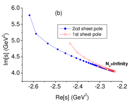
Figure 2: a) The $\sigma$ pole trajectory on $s$ plane from [1,2] $\rm{Pad\acute{e}}$ amplitude; b) poles on different sheets cancel each other in large $N_{c}$ limit. The starting points of the two trajectories correspond to arbitrary values of $N_{c}$ rather than 3.

4 The PKU approach

In this section we study the pole trajectory in the PKU parametrization[8] form in the $IJ=00$ channel. The advantage of using the PKU parametrization form comparing with the Padé approximation is that it avoids the problem of the violation of analyticity by the latter.[16] We firstly expand $T$ matrix from SU(2) $O(p^{4})$ ChPT amplitude at $2\pi$ threshold,

$$T^{ChPT}(s)=t_{0}+it_{1}(\frac{s-4m_{\pi}^{2}}{m_{\pi}^{2}})^{\frac{1}{2}}+t_{2}(\frac{s-4m_{\pi}^{2}}{m_{\pi}^{2}})+it_{3}(\frac{s-4m_{\pi}^{2}}{m_{\pi}^{2}})^{\frac{3}{2}}+\cdot\cdot\cdot$$ (9)

where those coefficients $t_{i}$ are functions of the low energy constants. On the other side the $T$ matrix in the PKU parametrization form is parametrized as,[8]

$$T(s)=(\frac{-s+M^{2}+i\rho(s)sG}{-s+M^{2}-i\rho(s)sG}e^{2i\rho(s)f(s)}-1)/(2i\rho(s))$$ (10)

where we have assumed one pole (and hence the $\sigma$ pole) dominance. To expand above parameterized $T$ matrix at $4m_{\pi}^{2}$:

$$T(s)=C_{0}+i\frac{C_{1}}{m_{\pi}}(s-4m_{\pi}^{2})^{1/2}+\frac{C_{2}}{m_{\pi}^{2}}(s-4m_{\pi}^{2})+O((s-4m_{\pi}^{2})^{3/2})\ ,$$ (11)

The background contribution $f$ is obtained from ChPT and the threshold expansion,

$$f(s)=f_{0}+\frac{f_{1}}{m_{\pi}^{2}}(s-4m_{\pi}^{2})+\frac{f_{2}}{m_{\pi}^{4}}(s-4m_{\pi}^{2})^{2}+O((s-4m_{\pi}^{2})^{3})\ .$$ (12)

Matching Eq. (9) and Eq. (11) at each order leads to for example the following equations:

$$C_{0}=t_{0}\ ,\,\,\,C_{2}=t_{2}\ ,\,\,\,C_{4}=t_{4}\ .$$ (13)

There are only two parameters (for one pole) with 3 equations and the system is over determined. Therefore 3 different solutions of the $\sigma$ pole exist depending on which two out of 3 equations we choose. Nevertheless it is found that the three solutions are highly compatible for realistic situation when $N_{c}=3$, the approximate solution is roughly $M_{\sigma}\simeq 460MeV$, $\Gamma_{\sigma}\simeq 470MeV$, which agrees rather well with more rigorous calculations[4, 5]. In fact, one can prove that the 3 solutions become unique in the large $N_{c}$ and chiral limit. Solving $C_{0}=t_{0}$ one gets

$$G=-\frac{1}{4m_{\pi}^{2}}(-4m_{\pi}^{2}+{M^{2}})({f_{0}}-{t_{0}})\ .$$ (14)

We can get $M$ by solving $C_{2}=t_{2}$,

$$M=\frac{2m_{\pi}\,{\sqrt{{{f_{0}}}^{3}+12\,{f_{1}}-3\,{{f_{0}}}^{2}\,{t_{0}}+3\,{f_{0}}\,{{t_{0}}}^{2}-3\,{{t_{0}}}^{3}-12\,{t_{2}}}}}{{\sqrt{-3\,{f_{0}}+{{f_{0}}}^{3}+12\,{f_{1}}+3\,{t_{0}}-3\,{{f_{0}}}^{2}\,{t_{0}}+3\,{f_{0}}\,{{t_{0}}}^{2}-3\,{{t_{0}}}^{3}-12\,{t_{2}}}}}$$ (15)

In the large $N_{c}$ limit the above solution can be simplified as,

$$G = -\frac{1}{4m_{\pi}^{2}}(-4m_{\pi}^{2}+{M^{2}})(f_{0}-{t_{0}})$$

$$M = \frac{4m_{\pi}\,{\sqrt{{t_{2}}}}}{{\sqrt{f_{0}-{t_{0}}+4\,{t_{2}}}}}$$ (16)

Where up to $O(p^{4})$, $t_{0}={7m_{\pi}^{2}\over{{32\pi F_{\pi}}}^{2}}+\frac{m_{\pi}^{4}}{2{{{{{\pi F}}_{\pi}}}^{4}}}(15L_{2}+5L_{3}+L_{5}+5L_{8})$ , $t_{2}={m_{\pi}^{2}\over{{16\pi F_{\pi}}}^{2}}+{m_{\pi}^{4}\over 2{{{{\pi F}_{\pi}}}^{4}}}(10L_{2}+4L_{3}+L_{5})$, $f_{0}=-|T^{\chi PT}(0)|=-\frac{m_{\pi}^{2}}{32{{{{\pi F}_{\pi}}}^{2}}}+\frac{m_{\pi}^{4}}{6{{{{\pi F}_{\pi}}}^{4}}}(25L_{2}+11L_{3}-9L_{5}+15L_{8})$. It is verified that the above solution satisfies the equation $C_{4}=t_{4}$ in the large $N_{c}$ and chiral limit and agrees exactly with Eq.(3). From Eq.(15), we see that $M$ is $O(1)$ and $G$ is $O(1/N_{c})$.[17]

The pole trajectory with respect to the variation of $N_{c}$ can be traced numerically. The result is found to be very similar to [1,1] $\rm{Pad\acute{e}}$ result. The plot of the pole trajectory can be found in Ref. [8]

5 Summary

Using Padé approximation and the unitarization approach developed by our group, we discuss the $N_{c}$ dependence of the mass and width of the $\sigma$ resonance. This paper is a supplementary to Ref. [6]. Though the very existence of the $\sigma$ pole has been firmly established, it’s dynamical nature remains mysterious. We hope the discussion given here will be of some use towards a deeper understanding on its origin. Our investigation seems to support the picture that the $\sigma$ pole is a conventional $\bar{q}q$ meson environed by heavy pion clouds. However the possibility that the $\sigma$ pole moves to the negative real axis as revealed by our investigation makes the topic interesting, which certainly deserves further investigations. Another scenario which can not be excluded is that the $\sigma$ pole moves to $\infty$, this situation may happen when the $\sigma$ pole does not contribute to the $L_{i}$ parameters of the low energy effective theory. We emphasize here that we disagree with the suggestion that the $\sigma$ pole is a $\bar{q}\bar{q}qq$ state. In fact, under mild assumptions, it is demonstrated that no resonance state with $M\sim O(1)$, $\Gamma\sim O(1)$ could exist, and therefore a tetra quark state does not exist in general.[6, 18] This result is a step forward to the previous understanding on such issue.[13]

References

- [1] S. Eidelman et al. (the Particle data group), Phys. Lett. B592(2004)1.
- [2] Z. G. Xiao and H. Q. Zheng, Nucl. Phys. A695(2001)273.
- [3] E791 collaboration, E.M. Aitala et al., Phys. Rev. Lett. 86(2001)770; BES collaboration, M. Ablikim et al., Phys. Lett. B598(2004)149; J. Z. Bai et al., High Energy Phys. Nucl. Phys. 28 (2004) 215.
- [4] G. Colangelo, J. Gasser and H. Leutwyler, Nucl. Phys. B603(2001)125.
- [5] Z. Y. Zhou et al., JHEP02(2005)043.
- [6] Z. G. Xiao and H. Q. Zheng, preprint hep-ph/0502199.
- [7] H. Q. Zheng et al., Nucl. Phys. A733(2004)235; H. Q. Zheng, hep-ph/0304173.
- [8] Z. X. Sun et al., talk given at 6th Conference on Quark Confinement and the Hadron Spectrum, Villasimius, Sardinia, Italy, 21-25 Sep 2004, hep-ph/0411375.
- [9] G. Y. Qin et al., Phys. Lett. B452(2002)89.
- [10] V. Bernard, N. Kaiser, and U. G Meissner, Phys. Rev. D 43, 2757(1991); Nucl. Phys. B357, 129(1991); Phys. Rev. D44, 3698(1991).
- [11] J. Pelaez, Phys. Rev. Lett. 92(2004)102001.
- [12] J. Gasser and H. Leutwyler, Nucl. Phys. B250(1985)465.
- [13] E. Witten, Nucl. Phys. B 160(1979)57; S. Coleman, in Aspects of Symmetry, Cambridge University Press 1985; For a recent review, see, R. F. Lebed, Czech. J. Phys. 49(1999)1273.
- [14] J. Bijnens et al., Phys. Lett. B374(1996)210; J. Bijnens et al., JHEP 9902(1999)020; J. Bijnens et al., Annals Phys. 280(2000)100.
- [15] J. Bijnens et al., Nucl. Phys. B508(1997)263, Erratum: ibid, B517(1998)639.
- [16] Notice that poles does not automatically appear on the physical sheet in here. It is the solutions of Eq. (13) tells on which sheet poles locate.
- [17] Thus does not go to . But this is a consequence of the assumption that the pole doiminates low energy physics at large .
- [18] H. Q. Zheng talk given at MENU2004, hep-ph/0411025.