Pentaquark Decay Width in QCD Sum Rules

Abstract

In a diquark-diquark-antiquark picture of the pentaquark we study the decay $\Theta\rightarrow K^{+}n$ within the framework of QCD sum rules. After evaluation of the relevant three-point function, we extract the coupling $g_{\Theta nK}$ which is directly related to the pentaquark width. Restricting the decay diagrams to those with color exchange between the meson-like and baryon-like clusters reduces the coupling constant by a factor of four. Whereas a small decay width might be possible for a positive parity pentaquark, it seems difficult to explain the measured width for a pentaquark with negative parity.

I Introduction

The possible existence of the pentaquark is one of the most exiting questions in current particle phenomenology. So far, more than ten experiments have found evidence for the existence of a pentaquark state PosResults . However, an almost equal number of experiments do not see any signal at the mass of the pentaquark NegResults . The experiments who reported positive results work in a medium energy range and have limited statistics. No pentaquark was seen in high energy experiments, however, the production mechanism is unclear and it is very difficult give an estimate for the production rate. Higher statistics experiments will be needed to clarify the existence of this new hadronic state. A review on the present experimental status can e.g. be found in dzi .

These investigations have triggered an intense theoretical activity and for an overview on the theoretical status we refer to reader to theory . One of the most puzzling characteristics of the pentaquark is its extremely small width (much) below 10 MeV which poses a serious challenge to all theoretical models. Indeed, in the conventional uncorrelated quark model the expected width is of the order of several hundred MeV, since the strong decay $\Theta^{+}\,\rightarrow KN$ is Okubo-Zweig-Iizuka (OZI) super-allowed. Many explanations for this narrow width have been advanced carlson ; Stech ; oga ; ricanari . A suggestive way to explain the small width is by the assumption of diquark clustering Jaffe:2003sg . The formation of diquarks presents an important concept and has direct phenomenological impact Diquarks .

In this work we calculate the pentaquark decay width within the framework of QCD sum rules. The basis of the sum rules was laid in SRbasis and their extension to baryons was developed in SRbaryons . The assumptions of the model are incorporated by an appropriate current. The sum rules are directly based on QCD and keep the analytic dependence on the input parameters. Several sum rule calculations have been performed for the mass of the pentaquark containing a strange zhu ; mnnr ; oka ; eiden or charm suhong_charm quark. These calculations are based on two-point functions with different interpolating currents. Surprisingly, all these determinations give similar masses with reasonable values. A common problem of all determinations is the large continuum contribution which has its origin in the high dimension of the interpolating currents and results in a large dependence on the continuum threshold. Another problem is the irregular behavior of the operator product expansion (OPE), which is dominated by higher dimension operators and not by the perturbative term as it should be.

Here we present for the first time a sum rule determination for decay width based on a three-point function for the decay $\Theta\to nK^{+}$. In this way we can extract the coupling $g_{\Theta nK}$ which is directly related to the pentaquark width. To describe the pentaquark we use the diquark-diquark-antiquark model with one scalar and one pseudoscalar diquark in a relative S-wave.

In oga ; ricanari it has been argued that such a small decay width can only be explained if the pentaquark is a genuine 5-quark state, i.e., it contains no color singlet meson-baryon contributions and thus color exchange is necessary for the decay. They start from simple observations concerning symmetries of the quark currents and the properties of the basic decay diagram as shown in Fig. 1. The analysis presented both in oga and in ricanari is only qualitative and arrives at the conclusion that, for a particular choice of the pentaquark current and assuming that it is a genuine 5-quark state, the decay width is given by $\Gamma_{\Theta}\simeq\alpha^{2}_{s}\,<0|\overline{q}q|0>^{2}$. In this expression $\alpha^{2}_{s}$ appears due to a hard gluon exchange and is therefore small. The narrowness of the pentaquark width can then be attributed to chiral symmetry breaking and the non-trivial color structure of the pentaquark which requires the exchange of, at least, one gluon. In this work we will also test quantitatively the hypothesis put forward in oga ; ricanari to see whether this mechanism is sufficient to explain the small width. The effect of chiral symmetry breaking for two chirally different diquarks in a relative S-wave was estimated in Stech . It was concluded that chiral breaking alone is not sufficient to explain a very small pentaquark width and our investigation will support this finding.

II The correlation function

Whereas the QCD sum rule determinations for the mass of the pentaquark are based on two-point functions zhu ; mnnr ; oka ; eiden , an investigation of the decay width requires a three-point function which we define as

$$\Gamma(p,p^{,}) = \int d^{4}x\,d^{4}y\,e^{-iqy}\,e^{ip^{,}x}\,\Gamma(x,y)\,,$$

$$\Gamma(x,y) = \langle 0|T\{\eta_{N}(x)j_{K}(y)\bar{\eta}_{\Theta}(0)\}|0\rangle\,,$$ (1)

where $\eta_{N}$, $j_{K}$ and $\eta_{\Theta}$ are the interpolating fields associated with neutron, kaon and $\Theta$, respectively.

II.1 The phenomenological side

We now consider the expression (II) in terms of hadronic degrees of freedom and write the phenomenological side of the sum rule. Though in oka it has been argued that a scalar-pseudoscalar diquark model is more likely related to a negative parity pentaquark, in this work we make no assumption about the parity of the $\Theta$ and investigate the consequences for both cases. Treating the kaon as a pseudoscalar particle, the interaction between the three hadrons is described by the following Lagrangian density:

$${\cal L} = ig_{\Theta nK}\bar{\Theta}\gamma_{5}Kn\quad\mbox{for $P=+$}$$

$${\cal L} = ig_{\Theta nK}\bar{\Theta}Kn\quad\ \ \ \mbox{for $P=-$}$$ (2)

Writing the correlation function (II) in momentum space and inserting complete sets of hadronic states we obtain

$$\Gamma(p,p^{\prime})=\sum_{s,s^{\prime}}\,-i\,\frac{\langle 0|\eta_{N}|n(p^{\prime},s^{\prime})\rangle V(p,p^{\prime})\langle K(q)|j_{K}|0\rangle\langle\Theta(p,s)|\bar{\eta}_{\Theta}|0\rangle}{(p^{\prime 2}-m_{N}^{2})(q^{2}-m_{K^{+}}^{2})(p^{2}-m_{\Theta}^{2})},$$ (3)

with

$$-i\,V(p,p^{\prime}) = <n(p^{\prime},s^{\prime})|\Theta(p,s)K(q)>\,,$$

$$\langle 0|\eta_{N}|n(p^{\prime},s^{\prime})\rangle = \lambda_{N}u^{s^{\prime}}(p^{\prime})\,,$$

$$\langle K(q)|j_{K}|0\rangle = \lambda_{K}\,,$$

$$\langle\Theta(p,s)|\bar{\eta}_{\Theta}|0\rangle = \lambda_{\Theta}\bar{u}^{s}(p)\quad\ \ \ \ \ \mbox{for $P=+$}$$

$$\langle\Theta(p,s)|\bar{\eta}_{\Theta}|0\rangle = -\lambda_{\Theta}\bar{u}^{s}(p)\gamma_{5}\quad\mbox{for $P=-$}$$ (4)

where the spinors are normalized according to

$$\sum_{s=1,2}\,u^{s}(p)\bar{u}^{s}(p)=\not{\!p}+m.$$ (5)

Using the simple Feynman rules derived from (II.1) we can rewrite $V(p,p^{\prime})$ as

$$V(p,p^{\prime}) = -\,g_{\Theta nK}\bar{u}^{s^{\prime}}(p^{\prime})\gamma_{5}u^{s}(p)\quad\mbox{for $P=+$}$$

$$V(p,p^{\prime}) = -\,g_{\Theta nK}\bar{u}^{s^{\prime}}(p^{\prime})u^{s}(p)\quad\ \ \ \mbox{for $P=-$}$$ (6)

The coupling constants $\lambda_{N}$ and $\lambda_{\Theta}$ can be determined from the QCD sum rules of the corresponding two-point functions. $\lambda_{K}$ is related to the kaon decay constant through

$$\lambda_{K}=\frac{f_{K}m_{K}^{2}}{m_{u}+m_{s}}\,.$$ (7)

Combining the expressions above we arrive at

$$\Gamma(p,p^{\prime})=-ig_{\Theta nK}\lambda_{\Theta}\lambda_{N}\lambda_{K}\frac{(\not{\!p^{\prime}}+m_{N})(\not{\!p}\pm m_{\Theta})\gamma_{5}}{(p^{\prime 2}-m_{N}^{2})(q^{2}-m_{K^{+}}^{2})(p^{2}-m_{\Theta}^{2})}\,\,+\,\,\mbox{continuum}$$ (8)

where the upper (lower) sign corresponds to a negative (positive) parity pentaquark. Finally, writing all the Dirac structures explicitly, the phenomenological correlator is given by

$$\Gamma_{phen}(p,p^{\prime})=\frac{-g_{\Theta nK}\lambda_{\Theta}\lambda_{N}\lambda_{K}}{(p^{\prime 2}-m_{N}^{2})(q^{2}-m_{K^{+}}^{2})(p^{2}-m_{\Theta}^{2})}\Gamma_{E}\,\,+\,\,\mbox{continuum}$$ (9)

with

$$\Gamma_{E}=\sigma^{\mu\nu}\gamma_{5}q_{\mu}p^{\prime}_{\nu}-im_{N}\not{\!q}\gamma_{5}+i(\pm m_{\Theta}+m_{N})\not{\!p^{\prime}}\gamma_{5}+i(p^{\prime 2}\pm m_{\Theta}m_{N}-qp^{\prime})\,.$$ (10)

We shall work with the $\sigma^{\mu\nu}\gamma_{5}q_{\mu}p^{\prime}_{\nu}$ structure because, as it was shown in gamma5 , this structure gives results which are less sensitive to the coupling scheme on the phenomenological side, i.e., to the choice of a pseudoscalar or pseudovector coupling between the kaon and the baryons. The continuum part contains the contributions of all possible excited states. They require a special treatment and we will discuss these terms separately after presenting the theoretical contributions.

II.2 The theoretical side

We now come back to (II) and write the interpolating fields in terms of quark degrees of freedom as

$$j_{K}(y) = \bar{s}(y)i\gamma_{5}u(y)\,,$$

$$\eta_{N}(x) = \epsilon^{abc}({d}^{T}_{a}(x)C\gamma_{\mu}d_{b}(x))\gamma_{5}\gamma^{\mu}u_{c}(x)\,,$$

$$\bar{\eta}_{\Theta}(0) = -\epsilon^{abc}\epsilon^{def}\epsilon^{cfg}{s}^{T}_{g}(0)C[\bar{d}_{e}(0)\gamma_{5}C\bar{u}^{T}_{d}(0)][\bar{d}_{b}(0)C\bar{u}^{T}_{a}(0)]\,.$$ (11)

The current of the pentaquark incorporates the assumption of a diquark-diquark-antiquark system with a scalar and pseudoscalar diquark. Inserting these currents into (II), the resulting expression can be written in the following form:

$$\Gamma_{th}(x,y) = 2i\epsilon^{abc}\epsilon^{def}\epsilon^{cfg}\epsilon^{a^{\prime}b^{\prime}c^{\prime}}\widetilde{\Gamma}(x,y)\,,$$

$$\widetilde{\Gamma}(x,y) = [N_{2}(x)-N_{1}(x)]K(y)\,,$$ (12)

with

$$N_{1}(x) = \gamma_{5}\gamma^{\beta}S_{c^{\prime}d}(x)CS^{T}_{a^{\prime}e}(x)C\gamma_{\beta}S_{b^{\prime}b}(x)\gamma_{5}\,,$$

$$N_{2}(x) = \gamma_{5}\gamma^{\beta}S_{c^{\prime}d}(x)\gamma_{5}CS^{T}_{a^{\prime}e}(x)C\gamma_{\beta}S_{b^{\prime}b}(x)\,,$$

$$K(y) = CS^{T}_{ha}(y)C\gamma_{5}CS^{T}_{gh}(-y,m_{s})C\,.$$ (13)

In order to proceed with the evaluation of the correlator (II) at the quark level, we need the quark propagator in the presence of quark and gluon condensates. Keeping track of the terms linear in the quark mass and taking into account quark and gluon condensates, we have

$$S_{ab}(x) = \langle 0|T[q_{a}(x)\overline{q}_{b}(0)]|0\rangle={i\delta_{ab}\over 2\pi^{2}x^{4}}\hbox to0.0pt{/\hss}{x}-{m_{q}\delta_{ab}\over 4\pi^{2}x^{2}}-{i\over 32\pi^{2}x^{2}}t^{A}_{ab}g_{\rm s}G^{A}_{\mu\nu}(\hbox to0.0pt{/\hss}{x}\sigma^{\mu\nu}+\sigma^{\mu\nu}\hbox to0.0pt{/\hss}{x})$$ (14)

$$- {\delta_{ab}\over 12}\langle{\overline{q}q}\rangle-{m_{q}\over 32\pi^{2}}t^{A}_{ab}g_{\rm s}G^{A}_{\mu\nu}\sigma^{\mu\nu}\ln(-x^{2})+{i\delta_{ab}\over 48}m_{q}\langle{\overline{q}q}\rangle\hbox to0.0pt{/\hss}{x}-{x^{2}\delta_{ab}\over 2^{6}\times 3}\langle{g_{\rm s}\overline{q}\sigma\!\cdot\!{\cal G}q}\rangle$$

$$+ {ix^{2}\delta_{ab}\over 2^{7}\times 3^{2}}m_{q}\langle{g_{\rm s}\overline{q}\sigma\!\cdot\!{\cal G}q}\rangle\hbox to0.0pt{/\hss}{x}-{x^{4}\delta_{ab}\over 2^{10}\times 3^{3}}\langle{\overline{q}q}\rangle\langle{{\displaystyle{g_{\rm s}^{2}G^{2}}}}\rangle\,-{x^{2}ln(-x^{2})m_{q}\delta_{ab}\over 2^{9}\times 3\pi^{2}}\langle{\overline{q}q}\rangle\langle{{\displaystyle{g_{\rm s}^{2}G^{2}}}}\rangle$$

where we have used the factorization approximation for the multi-quark condensates and we have used the fixed-point gauge. Inserting (14) into Eqs. (II.2) and these into (II.2), we arrive at a complicated function which is given schematically by the sum of the diagrams of Fig. 2. For any given Dirac structure this function can be written in a factorized form:

$$\Gamma_{th}(x,y)=H(x^{2})\cdot L(y^{2})\,.$$ (15)

After Fourier transformation, this leads to a similar separation in momentum space. The diagrams of Fig. 2 can then be expressed in terms of ${\widetilde{H}}(p^{\prime 2})$ and ${\widetilde{L}}(q^{2})$.

II.3 The continuum part and pole-continuum transitions

Let us consider the phenomenological side (9) and, following ioffe3 , rewrite it generically as a double dispersion relation:

$$\Gamma(q^{2},p^{2},p^{\prime 2})\,=\,\int_{0}^{\infty}\,ds\int_{0}^{\infty}\,du\,\frac{\rho(s,u,p^{2})}{(s-p^{\prime 2})(u-q^{2})}\,.$$ (16)

The double discontinuity can be written as the sum:

$$\rho(s,u,p^{2})\, = \,a(p^{2})\delta(s-m^{2}_{N})\delta(u-m^{2}_{K})\,+\,b_{1}(u,p^{2})\delta(s-m^{2}_{N})\,\theta(u-m^{2}_{K^{*}})\,$$ (17)

$$+ \,b_{2}(s,p^{2})\delta(u-m^{2}_{K})\,\theta(s-m^{2}_{N^{*}})\,+\,\rho_{cc}(s,u,p^{2})\theta(s-s_{0})\theta(u-u_{0})\,,$$

where the continuum thresholds are defined as

$$s_{0}\,=\,(m_{N}\,+\,\Delta_{N})^{2}\,\,\,\,\,\,\mbox{GeV}^{2}\,\,\,\,\,\,\,\,\,\,u_{0}\,=\,(m_{K}\,+\,\Delta_{K})^{2}\,\,\,\,\,\mbox{GeV}^{2}\,.$$ (18)

The terms proportional to $b_{1}$ and $b_{2}$ represent pole-continuum transitions where the pentaquark (in the ground state or in an excited state) decays into one ground state nucleon and one exited kaon or vice versa. Inserting (17) into (16) we can write

$$\Gamma(q^{2},p^{2},p^{\prime 2})\,=\,\Gamma_{pp}(q^{2},p^{2},p^{\prime 2})\,+\,\Gamma_{pc1}(q^{2},p^{2},p^{\prime 2})\,+\,\Gamma_{pc2}(q^{2},p^{2},p^{\prime 2})\,+\,\Gamma_{cc}(q^{2},p^{2},p^{\prime 2})\,,$$ (19)

where $\Gamma_{pp}$ comes from the first term in (17) and stands for the pole-pole part. The coefficient $a(p^{2})$ is obtained from Eq. (9) and we get

$$\Gamma_{pp}(q^{2},p^{2},p^{\prime 2})=-\frac{g_{\Theta nK}\lambda_{\Theta}\lambda_{N}\lambda_{K}}{(p^{2}-m_{\Theta}^{2})(p^{\prime 2}-m^{2}_{N})(q^{2}-m^{2}_{K})}\,.$$ (20)

The continuum-continuum term $\Gamma_{cc}$ can be obtained as usual, with the assumption of quark-hadron duality, from the double dispersion integral (16) using the theoretical expressions $\rho_{cc}(s,u,p^{2})\,=\,\rho_{th}(s,u,p^{2})$. We can also write a double dispersion integral for $\Gamma_{th}(q^{2},p^{2},p^{\prime 2})$ and, because of duality, $\Gamma_{cc}$ may be transferred to the theoretical side. This only changes the integration limits, so that the final theoretical side or right-hand side of the sum rule reads:

$$\Gamma_{rhs}(q^{2},p^{2},p^{\prime 2})\,=\,\Gamma_{th}(q^{2},p^{2},p^{\prime 2})\,-\,\Gamma_{cc}(q^{2},p^{2},p^{\prime 2})\,=\,\int_{0}^{s_{0}}\,ds\,\int_{0}^{u_{0}}\,du\,\frac{\rho_{th}(s,u,p^{2})}{(s-p^{\prime 2})(u-q^{2})}\,.$$ (21)

The pole-continuum transition terms are contained in $\Gamma_{pc1}$ and $\Gamma_{pc2}$. They can be explicitly written as

$$\Gamma_{pc1}(q^{2},p^{2},p^{\prime 2}) = \int_{0}^{\infty}\,ds\,\int_{m^{2}_{K^{*}}}^{\infty}\,\frac{b_{1}(u,p^{2})\,\delta(s-m^{2}_{N})\,du}{(s-p^{\prime 2})(u-q^{2})}=\int_{m^{2}_{K^{*}}}^{\infty}\,\frac{b_{1}(u,p^{2})\,du}{(m^{2}_{N}-p^{\prime 2})(u-q^{2})}\,,$$

$$\Gamma_{pc2}(q^{2},p^{2},p^{\prime 2}) = \int_{m^{2}_{N^{*}}}^{\infty}\,ds\,\int_{0}^{\infty}\,\frac{b_{2}(s,p^{2})\,\delta(u-m^{2}_{K})\,du}{(s-p^{\prime 2})(u-q^{2})}=\int_{m^{2}_{N^{*}}}^{\infty}\,\frac{b_{2}(s,p^{2})\,ds}{(m^{2}_{K}-q^{2})(s-p^{\prime 2})}\,.$$ (22)

In a usual three-point sum rule the quark lines in Fig. 1 connect all three particles, thus forming a triangle graph. After a double Borel transformation the continuum parts are exponentially suppressed compared to the pole contribution. One can then safely make the assumption of quark-hadron duality and parametrise the continuum by the double discontinuity of the theoretical part. However, as was first noticed in ioffe3 , diagrams where only two particles are connected contain a contribution in the pole-continuum transitions which is not exponentially suppressed compared to the pole contribution, even after double Borel transform. Therefore these contributions can be as large as the pole part and must be explicitly included in the sum rules. Since there is no theoretical tool to calculate the unknown functions $b_{1}(u,p^{2})$ and $b_{2}(s,p^{2})$ explicitly, one has to employ a parametrisation for these terms. We will use two different parametrisations: one with a continuous function for the $\Theta$ and one where the pole term is singled out. The difference between the two parametrisations should give an indication about the systematic error. In the analysis it will turn out that the pole-continuum terms are indeed of the same order as the pole contribution and should not be neglected.

Parametrisation A:

We shall assume that the functions $b_{1}$ and $b_{2}$ have the following form:

$$b_{1}(u,p^{2}) = \widetilde{b_{1}}(u)\int^{\infty}_{m_{\Theta}^{2}}d\omega\frac{b_{1}(\omega)}{\omega-p^{2}}\,,$$

$$b_{2}(s,p^{2}) = \widetilde{b_{2}}(s)\int^{\infty}_{m_{\Theta}^{2}}d\omega\frac{b_{2}(\omega)}{\omega-p^{2}}\,,$$ (23)

with continuous functions $b_{1,2}(w)$, starting from $m^{2}_{\Theta}$. The functions $\widetilde{b_{1}}(u)$ and $\widetilde{b_{2}}(s)$ describe the excitation spectra of the kaon and the nucleon, respectively. From experimental data we know that the nucleon has a very well established first excitation, the Roper resonance ($m_{N^{*}}=1440$ MeV), which is relatively far from the ground state. This suggests that the nucleon pole-continuum transitions will be saturated by the nucleon-Roper transitions. In order to simplify the calculations, we shall take advantage of this fact and use $\widetilde{b_{2}}(s)=\delta(s-m_{N^{*}}^{2})$. In the case of the kaon, surprisingly, no pseudoscalar higher excitation has been observed so far. Since the kaon excitations seem not to prefer any particular mass, we can not use the simplification applied above to the nucleon and therefore no assumption will be made on $\widetilde{b_{1}}(u)$. After Borel transform, the pole-continuum term contains one unknown constant factor which can be determined from the sum rules.

Parametrisation B:

In order to investigate the role played by the $\Theta$ continuum, we shall now explicitly force the phenomenological side to contain only the pole part of the $\Theta$, both in the pole-pole term and in the pole-continuum terms. This can formally be done by choosing $b_{1}(\omega)=b_{2}(\omega)=\delta(\omega-m_{\Theta}^{2})$. The functions then read:

$$b_{1}(u,p^{2}) = \frac{\widetilde{b_{1}}(u)}{m_{\Theta}^{2}-p^{2}}\,,$$

$$b_{2}(s,p^{2}) = \frac{\widetilde{b_{2}}(s)}{m_{\Theta}^{2}-p^{2}}\,.$$ (24)

In this case we have the $\Theta$ in the ground state and leave an open nucleon spectrum. Again, in the final expressions this gives an additional constant which can be calculated.

III The sum rule

The sum rule may be written inserting (II.2) into (II) and identifying it with (9). As can be seen explicitly in (10), each side of this identity contains a sum of different Dirac structures. The sum rule implies that the coefficients of each Dirac structure are equal both in the phenomenological side and in the theoretical side and therefore a sum rule is actually a set of equations. In principle we could work with any of the Dirac structures. As mentioned above, we shall work with the $\sigma^{\mu\nu}\gamma_{5}q_{\mu}p^{\prime}_{\nu}$ structure.

In order to suppress the condensates of higher dimension and at the same time reduce the influence of higher resonances we may perform on both sides of the sum rule a standard Borel transform SRbasis :

$$\Pi(M^{2})\equiv\lim_{n,Q^{2}\rightarrow\infty}\frac{1}{n!}(Q^{2})^{n+1}\left(-\frac{d}{dQ^{2}}\right)^{n}\Pi(Q^{2})\,,$$ (25)

($Q^{2}=-q^{2}$) with the squared Borel mass scale $M^{2}=Q^{2}/n$ kept fixed in the limit.

The above formulas are quite general. In order to proceed with the numerical analysis we have to decide how many Borel transforms we shall perform. In the case of the two-point function there is only one four momentum and thus only a single Borel transform is possible. In the case of the three-point function considered here, there are two independent momenta and we may perform either a single or a double Borel transform. If we were interested in computing the vertex form factor we would necessarily need to know the momentum dependence of the vertex function and this would imply making a Borel transform in two momentum variables (for example in $p$ and in $p^{\prime}$), leaving the other momentum ($q$) free. Since here we are mostly interested in the coupling constant we have more options which, in principle, should lead to the same result. We shall follow the procedure adopted in the past in similar situations. Following SRbasis and thiago we first consider the choice:

$$\mbox{(I)}\,\,\,\,\,\,\,\,\,\,q^{2}\,=\,0\,\,\,\,\,\,\,\,\ p^{2}\,=\,p^{\prime 2}$$ (26)

and perform a single Borel transform: $p^{2}\,=\,-P^{2}$ and $P^{2}\rightarrow M^{2}$. In this case we take $m_{K}^{2}\simeq 0$ and single out the $1/q^{2}$-terms. We may call this scheme the ”Kaon-Pole”-method. The second choice is:

$$\mbox{(II)}\,\,\,\,\,\,\,\,\,\,q^{2}\,\neq\,0\,\,\,\,\,\,\,\,\ p^{2}\,=\,p^{\prime 2}\,.$$ (27)

Here we perform two Borel transforms: $p^{2}\,=\,-P^{2}$ and $P^{2}\rightarrow M^{2}$ and also $q^{2}\,=\,-Q^{2}$ and $Q^{2}\rightarrow M^{{}^{\prime}2}$. We have also considered the choice $q^{2}\,=\,p^{2}\,=\,p^{\prime 2}\,=-P^{2}$, performing one single Borel transform ($P^{2}\rightarrow M^{2}$). This procedure was first advanced in nari86 , used later sometimes and has the advantage of simplifying the calculations. However, in the present calculation we were not able to find a stable sum rule. Moreover the equal momenta choice is less justified than the others, because when we set two momenta squared equal, this bears some connection with the masses or virtualities of the particles in the vertex. From this point of view, setting $p^{2}=p^{{}^{\prime}2}$ is quite reasonable, since the masses of the on-shell $\Theta$ and nucleon are not so different. On the other hand, the kaon mass squared is much smaller (and might even be set to zero) than $p^{2}$ and thus $q^{2}$ should not be close to it. Therefore in what follows the equal momenta choice will not be further considered.

In both cases considered above, there is no need of making extrapolations in order to obtain the coupling. Introducing the notation $G=-g_{\Theta nK}\lambda_{\Theta}\lambda_{N}\lambda_{K}$ and using (I) and (II) we obtain the following sum rules:

Method I: Kaon-Pole

$$\Gamma_{pp}(M^{2})+\Gamma_{pc2}(M^{2}) = \int_{0}^{s_{0}}ds\,\,\rho_{th}(s)\,\,e^{-s/M^{2}}\,,\quad\mbox{with}$$

$$\Gamma_{pp}(M^{2}) = G\frac{e^{-m^{2}_{\Theta}/M^{2}}-e^{-m^{2}_{N}/M^{2}}}{m^{2}_{\Theta}-m^{2}_{N}}\,,$$ (28)

and for the pole-continuum part we obtain

$$\Gamma_{pc2}(M^{2}) = A\,e^{-m^{2}_{N^{*}}/M^{2}}\quad\mbox{for parametrisation A}$$

$$\Gamma_{pc2}(M^{2}) = A\,e^{-m^{2}_{\Theta}/M^{2}}\quad\ \mbox{for parametrisation B}$$ (29)

In both parametrisations the term $\Gamma_{pc1}$ is exponentially suppressed and, as discussed in ioffe3 , has been neglected. $A$ is an unknown constant and can be determined from the sum rules.

Method II: Double Borel

$$\Gamma_{pp}(M^{2},M^{{}^{\prime}2})+\Gamma_{pc2}(M^{2},M^{{}^{\prime}2}) = \int_{0}^{u_{0}}\,du\,\int_{0}^{s_{0}}\,ds\,\rho_{th}(s,u)\,e^{-s/M^{2}}\,e^{-u/M^{{}^{\prime}2}}\,,\quad\mbox{with}$$

$$\Gamma_{pp}(M^{2},M^{{}^{\prime}2}) = G\,e^{-m^{2}_{K}/M^{{}^{\prime}2}}\,\frac{e^{-m^{2}_{\Theta}/M^{2}}-e^{-m^{2}_{N}/M^{2}}}{m^{2}_{\Theta}-m^{2}_{N}}$$ (30)

and

$$\Gamma_{pc2}(M^{2},M^{{}^{\prime}2}) = A\,e^{-m^{2}_{K}/M^{{}^{\prime}2}}\,e^{-m^{2}_{N^{*}}/M^{2}}\quad\mbox{for parametrisation A}$$

$$\Gamma_{pc2}(M^{2},M^{{}^{\prime}2}) = A\,e^{-m^{2}_{K}/M^{{}^{\prime}2}}\,e^{-m^{2}_{\Theta}/M^{2}}\quad\ \mbox{for parametrisation B}$$ (31)

Also in this case $\Gamma_{pc1}$ is exponentially suppressed.

IV Results

IV.1 Numerical input

In this section we determine the coupling constant $g_{\Theta nK}$. It is directly related to the experimentally measured $\Theta$ decay width through

$$\Gamma_{\Theta}=\frac{1}{8\pi m_{\Theta}^{3}}g_{\Theta nK}^{2}[(m_{N}\mp m_{\Theta})^{2}-m_{K}^{2}]\sqrt{\lambda(m_{\Theta}^{2},m_{N}^{2},m_{K}^{2})}\,,$$ (32)

where the upper (lower) sign is for positive (negative) parity and

$$\lambda(m_{\Theta}^{2},m_{N}^{2},m_{K}^{2})=(m_{\Theta}^{2}+m_{N}^{2}-m_{K}^{2})^{2}-4m_{\Theta}^{2}m_{N}^{2}\,.$$ (33)

The hadronic masses are $m_{N}=938$ MeV, $m_{N^{*}}=1440$ MeV, $m_{K}=493$ MeV and $m_{\Theta}=1540$ MeV. A decay width of $\Gamma_{\Theta}=10$ MeV then corresponds to the following coupling constants:

$$g_{\Theta nK} \simeq 3.0\quad\ \mbox{for $P=+$}$$

$$g_{\Theta nK} \simeq 0.43\quad\mbox{for $P=-$}$$ (34)

For each of the sum rules above (Eqs. (III) and (III)) we can take the derivative with respect to $1/M^{2}$ and in this way obtain a second sum rule. In each case we have thus a system of two equations and two unknowns ($G$ and $A$) which can then be easily solved. The results will depend on the numerical choices for all input parameters, including the strange quark mass, the condensates, the hadron masses and the choices of the continuum thresholds for the nucleon, $s_{0}$, and for the kaon, $u_{0}$.

In the numerical analysis of the sum rules we use the following values for the condensates: $\langle{\overline{q}q}\rangle=\,-(0.23\pm 0.02)^{3}\,\nobreak\,\mbox{GeV}^{3}$, $\langle\overline{s}s\rangle\,=0.8\,\langle{\overline{q}q}\rangle$, $<\bar{s}g_{s}{\bf\sigma.G}s>=m_{0}^{2}\,\langle{\bar{s}s}\rangle$ with $m_{0}^{2}=0.8\,\nobreak\,\mbox{GeV}^{2}$ and $\langle{{\displaystyle{g_{\rm s}^{2}G^{2}}}}\rangle=0.5~{}\nobreak\,\mbox{GeV}^{4}$. The gluon condensate has a large error of about a factor 2, but its influence on the analysis is relatively small. The couplings constants $\lambda_{N}$ and $\lambda_{\Theta}$ are taken from the corresponding two-point functions:

$$\lambda_{N}=(2.4\pm 0.2)\times 10^{-2}\,\mbox{GeV}^{3}\,,\,\,\,\,\,\,\,\,\,\,\lambda_{\Theta}=(2.4\pm 0.3)\times 10^{-5}\,\mbox{GeV}^{6}\,.$$ (35)

The coupling $\lambda_{K}$ is obtained from (7) with $f_{K}=160$ MeV, $m_{s}=100$ MeV and $m_{u}=5$ MeV:

$$\lambda_{K}=0.37\,\mbox{GeV}^{2}\,.$$ (36)

IV.2 Color-connected and color-disconnected diagrams

As can be seen in Fig. 1, the generic decay diagram in terms of quarks has two ”petals”, one associated with the kaon and the other with the nucleon. In Fig. 2 this picture is completed with the inclusion of all the relevant condensates. Among these OPE diagrams there are two distinct subsets. In the first (from 2a to 2g) there is no gluon line connecting the petals and therefore no color exchange. A diagram of this type we call color-disconnected. In the second subset of diagrams (2h, 2i and 2j) we have color exchange. If there is no color exchange, the final state containing two color singlets was already present in the initial state, before the decay, as noticed in morimatsu . In this case the pentaquark had a component similar to a $K-n$ molecule. In the second case the pentaquark was a genuine 5-quark state with a non-trivial color structure. We may call this type of diagram a color-connected (CC) one. In our analysis we write sum rules for both cases: all diagrams and only color connected. The former case is standard in QCDSR calculations and therefore we shall omit details and present only the results. The latter case implies that the pentaquark is a genuine 5-quark state and the evaluation of $g_{\Theta nK}$ will thus be based only on the CC diagrams. In this way we can test whether the assumption of the pentaquark being a genuine 5-quark state is sufficient to explain such a small decay width.

IV.3 Numerical analysis

In order to proceed with the numerical analysis we must choose a sum rule window for the Borel parameters $M$ and $M^{\prime}$. To ensure the convergence of the OPE we use values above 1 GeV. The upper limit is given by the condition that the continuum contribution should not be much larger than 50%. Thus we use a range of $1\,\mbox{\rm GeV}^{2}<M^{2},M^{\prime 2}<1.5\,\mbox{\rm GeV}^{2}$. Since the strange mass is small, the dominating diagram is Fig. 2b of dimension three with one quark condensate.

We have found out that the contribution from the pole-continuum part is of a similar size as the pole part. For lower values of $M$ around 1 GeV², the pole contribution dominates, however, for larger values of $M^{2}$ the importance of the pole-continuum contribution grows and eventually becomes larger than the pole part. This is an additional reason to restrict the analysis to small values for the Borel parameters.

We have evaluated the sum rules for the coupling constant computed with all diagrams of Fig. 2 and we have found that they are very stable. In order to avoid repetition we do not show the corresponding curves of $g_{\Theta nK}$ as afunction of the Borel mass squared $M^{2}$. We give only the values of the coupling extracted at $M^{2}=1.5$ GeV² and $M^{\prime 2}=1$ GeV² in Table I. In what follows we shall present our results for the coupling constant $g_{\Theta nK}$ obtained with the color connected diagrams only. In Fig. 3 we show the coupling, given by the solution of the sum rule I A (III), as a function of the Borel mass squared $M^{2}$. Different lines show different values of the continuum threshold $\Delta_{N}$. As it can be seen, $g_{\Theta nK}$ is remarkably stable with respect to variations both in $M^{2}$ and in $\Delta_{N}$. In Fig. 4 we show the coupling obtained with the sum rule II A (III). We find again fairly stable results which are very weakly dependent on the continuum threshold. Comparing the results obtained with I A and II A, we see that they are consistent with each other within the errors inherent to the method of QCD sum rules. In Fig. 5 we show the results of the sum rule I B. In Fig. 6 we present the result of the sum rule II B. The meaning of the different lines is the same as in the previous figures. The results are similar to the cases before.

In Table 1 we present a summary of our results for $g_{\Theta nK}$ giving emphasis to the difference between the results obtained with all diagrams and with only the color-connected ones. For the continuum thresholds we have employed $\Delta_{N}=\Delta_{K}=0.5$ GeV.

case	$|g_{\Theta nK}|$ (CC)	$|g_{\Theta nK}|$ (all diagrams)
I A	0.71	2.59
II A	0.82	3.59
I B	0.84	3.24
II B	0.96	4.48

Table 1: $g_{\Theta nK}$ for various cases

For our final value of $g_{\Theta nK}$ we take an average of the sum rules IA-IIB. It is interesting to observe that the influence of the continuum threshold is relatively small, especially when compared to the corresponding two-point functions.

Considering the uncertainties in the continuum thresholds, in the coupling constants $\lambda_{K,N,\Theta}$ and in the quark condensate we we get an uncertainty of about 50%. Our final result then reads:

$$|g_{\Theta nK}|\mbox{(all diagrams)} = 3.48\,\pm 1.8\,,$$

$$|g_{\Theta nK}|\mbox{(CC)} = 0.83\,\pm 0.42\,.$$ (37)

Including all diagrams, the prediction for $\Gamma_{\Theta}$ is then 13 MeV (652 MeV) for a positive (negative) parity pentaquark. In the CC case we get a width of 0.75 MeV (37 MeV) for a positive (negative) parity pentaquark. One should keep in mind that higher dimensional condensates and higher order perturbative corrections could increase this prediction for the width. The parity of the pentaquark has not been experimentally determined. The measured value of the width is around 5-10 MeV both in the Kn channel (considered here) and in the Kp channel.

We see that it is difficult to obtain the measured decay width for a negative parity pentaquark.

V Summary and conclusions

We have presented a QCD sum rule study of the decay of the $\Theta^{+}$ pentaquark using a diquark-diquark-antiquark scheme with one scalar and one pseudoscalar diquark. Based on an evaluation of the relevant three-point function, we have computed the coupling constant $g_{\Theta nK}$. In the operator product expansion we have included all diagrams up to dimension 5. In this particular type of sum rule a complication arises from the pole-continuum transitions which are not exponentially suppressed after Borel transformation and must be explicitly included. The analysis was made for two different pole-continuum parametrisations and in two different evaluation schemes. The results are consistent with each other. In addition, we have tested the ideas presented in oga ; ricanari by including only diagrams with color exchange. Our final results are given in eq. (37).

We find that for a positive parity pentaquark a width much smaller than 10 MeV would indicate a pentaquark which contains no color-singlet meson-baryon contribution. For a negative parity pentaquark, even under the assumption that it is a genuine 5-quark state, we can not explain the observed narrow width of the $\Theta$. In Stech the pentaquark was investigated in a nonrelativistic quark model for a diquark-diquark-antiquark configuration with two scalar diquarks in a relative P-wave. It was found that a narrow width is difficult to achieve, unless the pentaquark has an uncommon spatial structure. It seems that from the theory side a very small pentaquark width is not impossible, but that the pentaquark has indeed to be in a special configuration to explain the observed decay width.

Acknowledgements: It is a pleasure to thank R.D. Matheus for instructive discussions. M.E is grateful to FAPESP for financial support (contract number 2004/08960-4) and also acknowledges the hospitality extended to him during his stay in Brazil. This work has been supported by CNPq and FAPESP (Brazil).

Figure 1: The basic diagram for the theoretical side of the sum rule.

Figure 2: The main diagrams which contribute to the theoretical side of the sum rule in the relevant structure. a) - g) are the color disconnected diagrams, whereas h) - j) are the color connected diagrams. The cross indicates the insertion of the strange mass.

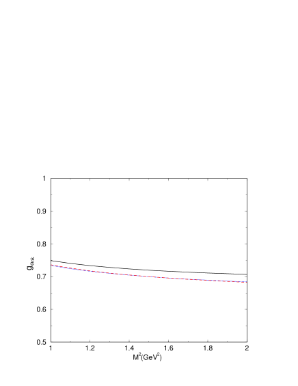
Figure 3: $|g_{\Theta nK}|$ in case I A with three different continuum threshold parameters. Solid line: $\Delta_{N}=0.5$ GeV, dotted line:$\Delta_{N}=0.4$ GeV, dash-dotted line: $\Delta_{N}=0.6$ GeV.

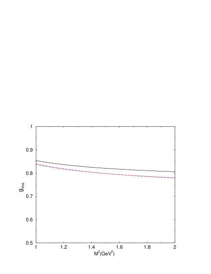
Figure 4: $|g_{\Theta nK}|$ in case II A. Solid line: $\Delta_{N}=0.5$ GeV. Dotted line: $\Delta_{N}=0.4$ GeV. Dashed line: $\Delta_{N}=0.6$ GeV. $M^{{}^{\prime}2}=1$ GeV².

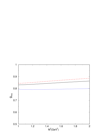
Figure 5: $|g_{\Theta nK}|$ in case I B with three different continuum threshold parameters. Solid line: $\Delta_{N}=0.5$ GeV, dotted line:$\Delta_{N}=0.4$ GeV, dash-dotted line: $\Delta_{N}=0.6$ GeV.

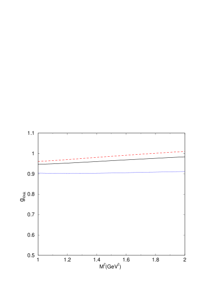
Figure 6: $|g_{\Theta nK}|$ in case II B. Solid line: $\Delta_{N}=0.5$ GeV. Dotted line: $\Delta_{N}=0.4$ GeV. Dashed line: $\Delta_{N}=0.6$ GeV. $M^{{}^{\prime}2}=1$ GeV².

References

- (1) T. Nakano et al. [LEPS Collaboration], Phys. Rev. Lett. 91 (2003) 012002; V. V. Barmin et al. [DIANA Collaboration], Phys. Atom. Nucl. 66 (2003) 1715; S. Stepanyan et al. [CLAS Collaboration], Phys. Rev. Lett. 91 (2003) 252001; J. Barth et al. [SAPHIR Collaboration], Phys. Lett. B 572 (2003) 127; V. Kubarovsky et al. [CLAS Collaboration], Phys. Rev. Lett. 92 (2004) 032001; (Erratum-ibid. 92 (2004) 049902); A. Airapetian et al. [HERMES Collaboration], Phys. Lett. B 585 (2004) 213; A. E. Asratyan, A. G. Dolgolenko and M. A. Kubantsev, Phys. Atom. Nucl. 67 (2004) 682. A. Aleev et al. [SVD Collaboration], arXiv:hep-ex/0401024; S. Chekanov et al. [ZEUS Collaboration], Phys. Lett. B 591 (2004) 7; M. Abdel-Bary et al. [COSY-TOF Collaboration], Phys. Lett. B 595 (2004) 127; C. Alt et al. [NA49 Collaboration], Phys. Rev. Lett. 92 (2004) 042003; A. Aktas et al. [H1 Collaboration], Phys. Lett. B 588 (2004) 17;
- (2) J. Z. Bai et al. [BES Collaboration], Phys. Rev. D 70 (2004) 012004; K. Abe et al. [BELLE Collaboration], arXiv:hep-ex/0409010; B. Aubert et al. [BABAR Collaboration], arXiv:hep-ex/0408064; K. T. Knopfle, M. Zavertyaev and T. Zivko [HERA-B Collaboration], J. Phys. G 30 (2004) S1363; D. O. Litvintsev [CDF Collaboration], arXiv:hep-ex/0410024; C. Pinkenburg [PHENIX Collaboration], J. Phys. G 30 (2004) S1201. Not all negative results have been published, for a review see dzi .
- (3) S. Kabana, hep-ex/0503019; A.R. Dzierba, C.A. Meyer and A.P. Szczepaniak, hep-ex/0412077; K. Hicks, hep-ex/0501018, hep-ex/0412048.
- (4) For recent reviews see: M. Oka, Prog. Theor. Phys. 112 (2004) 1; Shi-Lin Zhu, Int. J. Mod. Phys. LA19 (2004) 3439.
- (5) C.E. Carlson, C. D. Carone, H.J. Kwee, V. Nazaryan, Phys. Lett. B573 (2003) 101; R. Jaffe, F. Wilczek, Phys. Rev. Ḏ69 (2004) 114017 ; X.G. He, X.Q. Li, Phys. Rev. D70 (2004) 034030; Y. Oh, H. Kim, Phys. Rev. D70 (2004) 094022; T. Mehen, C. Schat, Phys. Lett. B588 (2004) 67; Y.R. Liu et al., Phys. Rev. D70 (2004) 094045; H.Y. Cheng, C.K. Chua, JHEP 0411 (2004)072 ; F.E. Close, J.J. Dudek, Phys. Lett. B586 (2004) 75; S.H. Lee, H. Kim, Y. Oh, hep-ph/0402135; H. Suganuma, F. Okiharu, T.T. Takahashi, H. Ichie, hep-ph/0412296; M. Karliner and H. Lipkin, hep-ph/0401072; F. Buccella and P.Sorba, hep-ph/0401083.
- (6) D. Melikhov and B. Stech, hep-ph/0501108, Phys. Lett. B 608 (2005) 59; D. Melikhov, S. Simula and B. Stech, Phys. Lett. B 594 (2004) 265;
- (7) B. L. Ioffe and A. G. Oganesian, JETP Lett. 80 (2004) 386; A. G. Oganesian, hep-ph/0410335.
- (8) R.D. Matheus, S. Narison, hep-ph/0412063.
- (9) R. L. Jaffe and F. Wilczek, Phys. Rev. Lett. 91 (2003) 232003; Eur. Phys. J. C 33 (2004) S38.
- (10) B. Stech, Phys. Rev. D 36 (1987) 975; M. Neubert and B. Stech, Phys. Lett. B 231 (1989) 477; M. Anselmino, E. Predazzi, S. Ekelin, S. Fredriksson and D. B. Lichtenberg, Rev. Mod. Phys. 65 (1993) 1199; H. G. Dosch, M. Jamin and B. Stech, Z. Phys. C 42 (1989) 167; M. Jamin and M. Neubert, Phys. Lett. B 238 (1990) 387.
- (11) M. A. Shifman, A. I. Vainshtein and V. I. Zakharov, Nucl. Phys. B 147 (1979) 385; Nucl. Phys. B 147 (1979) 448; L. J. Reinders, H. Rubinstein and S. Yazaki, Phys. Rept. 127 (1985) 1; S. Narison, World Sci. Lect. Notes Phys. 26 (1989) 1.
- (12) B. L. Ioffe, Nucl. Phys. B 188 (1981) 317; [Erratum-ibid. B 191 (1981) 591],Z. Phys. C 18 (1983) 67; Y. Chung, H. G. Dosch, M. Kremer and D. Schall, Phys. Lett. B 102 (1981) 175; Nucl. Phys. B 197 (1982) 55; H. G. Dosch, M. Jamin and S. Narison, Phys. Lett. B 220 (1989) 251.
- (13) S.-L. Zhu, Phys. Rev. Lett. 91 (2003) 232002.
- (14) R.D. Matheus, F.S. Navarra, M. Nielsen, R. Rodrigues da Silva and S.H. Lee, Phys. Lett. B578 (2004) 323; R.D. Matheus, F.S. Navarra, M. Nielsen, R. Rodrigues da Silva, Phys. Lett. B602 (2004) 185.
- (15) J. Sugiyama, T. Doi, M. Oka, Phys. Lett. B581 (2004) 167.
- (16) M. Eidemüller, Phys. Lett. B597 (2004) 314.
- (17) H. Kim, S.H. Lee, Y. Oh, Phys. Lett. B595 (2004) 293.
- (18) H. Kim, S.H. Lee and M. Oka, Phys. Lett. B453 (1999) 199; Phys. Rev. D60 (1999) 034007; F.O. Durães, F.S. Navarra, M. Nielsen, Phys. Lett. B498 (2001) 169; M.E. Bracco, F.S. Navarra, M. Nielsen, Phys. Lett. B454 (1999) 346.
- (19) R. Jaffe and F. Wilczek, Phys. Rev. Lett. 91 (2003) 232003 .
- (20) B. Ioffe and A. Smilga, Nucl. Phys. B232 (1984) 109.
- (21) T.V. Brito, F.S. Navarra, M. Nielsen and M.E. Bracco, Phys. Lett. B608 (2005) 69.
- (22) S. Narison, Phys. Lett. B175 (1986) 88.
- (23) Y. Kondo, O. Morimatsu, T. Nishikawa, hep-ph/0404285.