Abstract

A Monte-Carlo analysis on production and decay of supersymmetric charginos at a future photon-collider is presented. A photon collider offers the possibility of a direct branching-ratio measurement. In this study, the process $\gamma\gamma\rightarrow\tilde{\chi}_{1}^{+}\tilde{\chi}_{1}^{-}\rightarrow W^{+}W^{-}\tilde{\chi}_{1}^{0}\tilde{\chi}_{1}^{0}\rightarrow q\bar{q}q\bar{q}\tilde{\chi}_{1}^{0}\tilde{\chi}_{1}^{0}$ has been considered for a specific mSUGRA scenario. Various backgrounds and a parameterised detector simulation have been included. Depending on the centre-of-mass energy, a statistical error for the directly measurable branching ratio BR(${\tilde{\chi}_{1}^{\pm}}\rightarrow{\tilde{\chi}_{1}^{0}}W^{\pm}$) of up to 3.5% can be reached.

1 Introduction

An option for the future Linear Collider project is the photon collider [1, 2]. Such a collider provides the possibility of studying photon-photon collisions up to 80% of the $e^{-}e^{-}$ centre of mass energy. If Supersymmetry is realized in nature, then also supersymmetric particles can be produced and investigated at such a facility. The photon collider has the advantage that the production of charged particle pairs is determined by pure QED. This offers the possibility to directly measure the decay properties of supersymmetric particles, once their masses have been precisely measured at the $e^{+}e^{-}$-collider. In addition the production cross sections for charged particles are significantly larger at a photon collider than in $e^{+}e^{-}$ annihilation.

In this paper a Monte-Carlo analysis on production and decay of supersymmetric charginos $\chi^{\pm}_{1}$ is presented. The channel $\gamma\gamma\rightarrow\chi^{+}_{1}\chi^{-}_{1}\rightarrow W^{+}W^{-}\chi^{0}_{1}\chi^{0}_{1}\rightarrow q\bar{q}q\bar{q}\chi^{0}_{1}\chi^{0}_{1}$ has been studied, where each chargino decays into a $W^{\pm}$-boson and a neutralino $\chi^{0}_{1}$. The target was to estimate the statistical error in a direct measurement of the chargino branching ratio BR(${\tilde{\chi}_{1}^{\pm}}\rightarrow{\tilde{\chi}_{1}^{0}}W^{\pm}$). This was done for a mSUGRA scenario similar to SPS1a [3] and for two different beam energies ${\sqrt{s_{ee}}=500{\,\mathrm{Ge\kern-1.00006ptV}}}$ and ${\sqrt{s_{ee}}=600{\,\mathrm{Ge\kern-1.00006ptV}}}$. The main Standard Model backgrounds and a parameterised detector simulation have been included. The obtained efficiencies and purities are presented. Finally the relevance of the photon collider measurements in addition to $e^{+}e^{-}$ has been tested for the precision with which the Supersymmetry breaking parameters in the MSSM can be obtained.

2 Choice of a mSUGRA scenario

A general starting point for the choice of mSUGRA parameters is the SPS1a scenario [3]. However, in SPS1a the chargino decays almost entirely into a stau and a neutrino ${\tilde{\chi}_{1}^{\pm}}\rightarrow{\tilde{\tau}}^{\pm}_{1}\nu_{\tau}$, leaving only a small branching ratio of the decay $\chi^{\pm}_{1}\rightarrow W^{\pm}\chi^{0}_{1}$ [4]. For this reason the mSUGRA parameters have been slightly changed for this study in order to obtain a larger branching ratio for the decay into a $W^{\pm}$-boson and a neutralino. Table 1 shows the chosen values for the parameters. Only $m_{0}$ and $\tan\beta$ were modified with respect to SPS1a. This was done in such a way that $m_{\tilde{\chi}_{1}^{\pm}}$ and $m_{\tilde{\chi}_{1}^{0}}$ remained unchanged (Table 2). Thus the kinematical properties of the reaction $\gamma\gamma\rightarrow\chi^{+}_{1}\chi^{-}_{1}\rightarrow W^{+}W^{-}\chi^{0}_{1}\chi^{0}_{1}$ are the same as for the SPS1a case. However, $m_{{\tilde{\tau}}_{1}}$ changed as well as the branching ratio BR(${\tilde{\chi}_{1}^{\pm}}\rightarrow{\tilde{\chi}_{1}^{0}}W^{\pm}$) which is increased from 7% to 26%. This has been considered as a more reasonable number for an analysis of the ${\tilde{\chi}_{1}^{\pm}}\rightarrow{\tilde{\chi}_{1}^{0}}W^{\pm}$ decay.

Scenario	$m_{0}$	$m_{1/2}$	$A_{0}$	$\tan\beta$	sign $\mu$
SPS1a	$100{\,\mathrm{Ge\kern-1.00006ptV}}$	$250{\,\mathrm{Ge\kern-1.00006ptV}}$	$-100{\,\mathrm{Ge\kern-1.00006ptV}}$	$10$	$+1$
this study	$130{\,\mathrm{Ge\kern-1.00006ptV}}$	$250{\,\mathrm{Ge\kern-1.00006ptV}}$	$-100{\,\mathrm{Ge\kern-1.00006ptV}}$	$9$	$+1$

Table 1: The values of the mSUGRA parameters for SPS1a and the scenario used in this study.

Observable	SPS1a	this study
$m_{\tilde{\chi}_{1}^{\pm}}$	$180.4{\,\mathrm{Ge\kern-1.00006ptV}}$	$180.4{\,\mathrm{Ge\kern-1.00006ptV}}$
$m_{\tilde{\chi}_{1}^{0}}$	$95.6{\,\mathrm{Ge\kern-1.00006ptV}}$	$95.6{\,\mathrm{Ge\kern-1.00006ptV}}$
$m_{{\tilde{\tau}}_{1}}$	$134.4{\,\mathrm{Ge\kern-1.00006ptV}}$	$158.8{\,\mathrm{Ge\kern-1.00006ptV}}$
BR(${\tilde{\chi}_{1}^{\pm}}\rightarrow{\tilde{\tau}}^{\pm}_{1}\nu_{\tau}$)	91.9%	72.4%
BR(${\tilde{\chi}_{1}^{\pm}}\rightarrow{\tilde{\chi}_{1}^{0}}W^{\pm}$)	7.2%	26.2%

Table 2: Chargino, neutralino and stau masses and the chargino branching ratios for SPS1a and the parameter choice used in this study. The numbers were calculated with ISAJET 7.67 [5].

3 The photon collider

The photon collider ($\gamma\gamma$-collider) is an option for the next Linear Collider project [2]. The idea is to create high energetic photons by scattering accelerated electrons on a focused laser beam. For this purpose the positron beam is replaced by a second $e^{-}$-beam. The produced photon beams allow the study of photon collisions at energies and luminosities that are comparable to the $e^{+}e^{-}$-collider.

The energy spectrum of the scattered photons is shown in Fig. 1 (left) for an electron beam energy of $E(e^{-})=250{\,\mathrm{Ge\kern-1.00006ptV}}$ [7]. The spectrum is peaked at photon energies of about $70\%-80\%$ of the electron energy. The rise at low energies is due to multiple electron-photon interactions. The part of the spectrum above $y\approx 0.8E(e^{-})$ can be explained by nonlinear interactions of an electron with several laser photons [2]. Fig. 1 (right) shows the photon polarisation spectrum $\lambda(y)$: The high energetic photons are strongly circular polarised. This can be achieved, by using polarised electron and laser beams. Here, an electron polarisation of $85\%$ and a laser beam polarisation of $100\%$ was assumed.

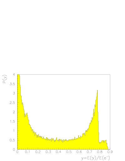
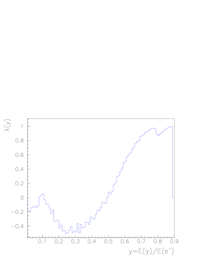
Figure 1: Energy distribution $P(y)$ of the produced photons (left) and photon polarisation $\lambda(y)$ (right) in dependence on $y$, which is the ratio of photon energy $E(\gamma)$ and beam-electron energy $E(e^{-})$.

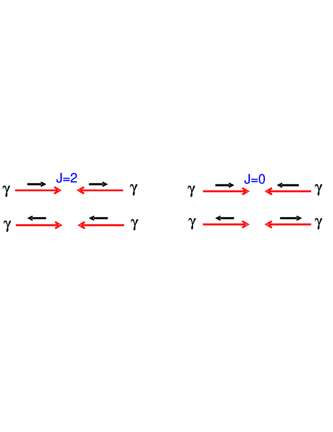
Figure 2: The possible alignments of the helicities (short arrows) of the colliding photons that lead to a total angular momentum of $J=2$ or $J=0$.

The circular polarisation of the photon beams offers two possible running modes for the $\gamma\gamma$-collider in terms of helicities (Fig. 2). One with a parallel and one with an anti-parallel alignment of the photon helicities. These correspond to an overall angular momentum of either $J=2$ or $J=0$ for the two-photon system. The luminosity spectrum and the polarisation in dependence of the two-photon centre-of-mass energy $\sqrt{s_{\gamma\gamma}}$ is shown in Fig. 3. It has been calculated with the program CAIN [6]. The total luminosity is ${\cal L}_{\gamma\gamma}=10\cdot 10^{34}cm^{-2}s^{-1}$ which corresponds to an integrated luminosity of $1000fb^{-1}$ per year. However the luminosity within the high energy peak (i.e. $\sqrt{s_{\gamma\gamma}}>300{\,\mathrm{Ge\kern-1.00006ptV}}$) is only ${\cal L}_{peak}=1.1\cdot 10^{34}cm^{-2}s^{-1}=100fb^{-1}/\mbox{year}$.

Figure 3: $\gamma\gamma$ luminosity spectrum $d{\cal L}/d\sqrt{s_{\gamma\gamma}}$ (left) and the fraction of the luminosity with $J=0$ (right) in dependence of $\sqrt{s_{\gamma\gamma}}$ for a centre-of-mass energy of the two electron beams of $\sqrt{s_{ee}}=500{\,\mathrm{Ge\kern-1.00006ptV}}$.

Compared to the $e^{+}e^{-}$-collider, a photon collider cannot provide monochromatic beams. This makes event analyses harder, since the collision energy, which is important for kinematic constraints, is an unknown variable here.

4 Chargino production

The pair production of charginos in photon collisions is described by pure QED. Fig. 4 shows the only leading order diagram for the $\gamma\gamma\rightarrow{\tilde{\chi}_{1}^{+}}{\tilde{\chi}_{1}^{-}}$ process.

Figure 4: Feynman diagram for $\gamma\gamma\rightarrow{\tilde{\chi}_{1}^{+}}{\tilde{\chi}_{1}^{-}}$

¿From this diagram the total cross section in the centre-of-mass system can be derived [8]:

$$\begin{split}\sigma_{p,\alpha\beta}=&\frac{e^{4}}{16\pi{E^{6}}}\biggl{\{}\left[m_{\tilde{\chi}}^{2}(2E^{2}-m_{\tilde{\chi}}^{2})+2E^{4}(1-\alpha\beta)\right]\ln{\frac{E+q}{m_{\tilde{\chi}}}}\\ &+Eq\left[2E^{2}-m_{\tilde{\chi}}^{2}-3E^{2}(1-\alpha\beta)\right]\biggr{\}}\end{split}$$ (1)

Where $E$ is the photon beam energy in the centre-of-mass system and $\alpha$,$\beta$ describe the helicity of the incoming photons. Furthermore $m_{\tilde{\chi}}$ and $q=(E^{2}-m_{\tilde{\chi}}^{2})^{1/2}$ are the chargino mass and momentum and $e$ is the elementary charge.

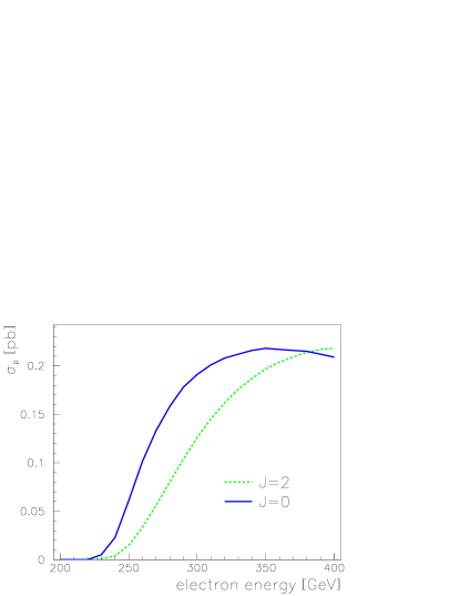
Figure 5: Left: $\sigma_{p,\alpha\beta}$ in dependence of $E$ for $J=0$ ($\alpha=\beta=\pm 1$) and $J=2$ ($\alpha=-\beta=\pm 1$), $m_{\tilde{\chi}}=180{\,\mathrm{Ge\kern-1.00006ptV}}$. Right: effective cross section $\sigma_{p}$ as a function of the electron beam energy $E_{e^{-}}=\frac{1}{2}\sqrt{s_{ee}}$ for $J=0$ and $J=2$.

Beside the photon energy and polarisation, the production cross section only depends on the charge and mass of the chargino. In Fig. 5 (left) the production cross section is plotted in dependence of the photon energy $E$ for the $J=2$ and $J=0$ mode. Because of parity conservation only the product $\alpha\cdot\beta=\pm 1$ is relevant. For energies less than $350{\,\mathrm{Ge\kern-1.00006ptV}}$ especially near the production threshold ($E=m_{\tilde{\chi}}=180{\,\mathrm{Ge\kern-1.00006ptV}}$) the cross section is larger for the $J=0$ mode, while this behaviour flips for higher energies. The maximum cross section is $\sigma\approx 2.1$ pb at $E\approx 230{\,\mathrm{Ge\kern-1.00006ptV}}$.

At a photon collider there are no monochromatic photon beams with fixed energy. The photons spread over a wide energy range. Thus the production cross section has to be convoluted with the luminosity spectrum $d{\cal L}/d\sqrt{s_{\gamma\gamma}}$ and the polarisation spectrum $\lambda(y)$ [8]:

$$\sigma_{p}(s_{\gamma\gamma})=\frac{1}{4}\sum_{\alpha,\beta=\pm 1}[1+\alpha\lambda(y_{1})][1+\beta\lambda(y_{2})]\sigma_{p,\alpha\beta}(s_{\gamma\gamma})$$ (2)

$$\sigma_{p}(s_{ee})=\int{d{\cal L}/d\sqrt{s_{\gamma\gamma}}\sigma_{p}(s_{\gamma\gamma}=y_{1}y_{2}s_{ee})d\sqrt{s_{\gamma\gamma}}}$$ (3)

Equation 2 describes the weighting of the cross section $\sigma_{p,\alpha\beta}$ with the mean helicities $\lambda(y_{1})$, $\lambda(y_{2})$ of the incoming photons. The resulting cross section $\sigma_{p}(s_{\gamma\gamma})$ is convoluted with the luminosity spectrum (eqn. 3). One obtains an effective production cross section $\sigma_{p}(s_{ee})$ for the overall process $e^{-}e^{-}\rightarrow\gamma\gamma\rightarrow{\tilde{\chi}_{1}^{+}}{\tilde{\chi}_{1}^{-}}$ in the $e^{-}e^{-}$ centre-of-mass system which is plotted in Fig. 5 (right) for the two different helicity modes $J=0,2$. It has been calculated with SHERPA [9]. For beam energies below $380{\,\mathrm{Ge\kern-1.00006ptV}}$ the $J=0$ configuration provides the larger cross section, therefore that mode is used in the following for this analysis. In the region, where the $J=0$ and $J=2$ mode are similar, we expect similar results for both modes. However the $J=2$ mode has not been studied in detail. In general the effective cross section is clearly smaller than the cross section for monochromatic beams. This is due to the fact that a major part of the colliding photons have too little energy to fulfil the threshold condition $s_{\gamma\gamma}=y_{1}y_{2}s_{ee}>(2m_{\tilde{\chi}})^{2}$.

$\sqrt{s_{ee}}=500$ GeV	$\sigma_{p}=64.7$ fb	$\approx 64.7\cdot 10^{3}$ ${\tilde{\chi}_{1}^{+}}{\tilde{\chi}_{1}^{-}}$ - pairs / year ($10^{7}s$)
$\sqrt{s_{ee}}=600$ GeV	$\sigma_{p}=198.0$ fb	$\approx 198\cdot 10^{3}$ ${\tilde{\chi}_{1}^{+}}{\tilde{\chi}_{1}^{-}}$ - pairs / year ($10^{7}s$)

Table 3: Values for the effective cross section $\sigma_{p}$ and the number of produced ${\tilde{\chi}_{1}^{+}}{\tilde{\chi}_{1}^{-}}$-pairs per year for $J=0$.

It should be stressed that this effective cross section is not a cross section in the conventional sense, since it implicitly contains information about the luminosity spectrum. In order to obtain the number of produced chargino pairs per year, $\sigma_{p}(s_{ee})$ has to be multiplied with the integrated photon luminosity of ${\cal L}_{\gamma\gamma}^{int}=1000fb^{-1}$. This leads to $\approx 64.7\cdot 10^{3}$ chargino pairs per year for a beam energy of $E_{e^{-}}=250{\,\mathrm{Ge\kern-1.00006ptV}}$ (i.e. $\sqrt{s_{ee}}=500{\,\mathrm{Ge\kern-1.00006ptV}}$) and $\approx 198\cdot 10^{3}$ pairs for $\sqrt{s_{ee}}=600{\,\mathrm{Ge\kern-1.00006ptV}}$ (Table 3). So at $600{\,\mathrm{Ge\kern-1.00006ptV}}$ there are about three times more produced chargino pairs than for $500{\,\mathrm{Ge\kern-1.00006ptV}}$.

5 Signal and background simulation

For the calculation of cross sections and the simulation of signal and background events the generic event generator SHERPA was used [9]. This program is based on the matrix-element generator AMEGIC [10] and allows to simulate processes with up to six particles in the final state. SHERPA also supports Supersymmetry and uses ISAJET 7.67 [5] for the generation of the mSUGRA particle spectrum. The photon spectrum is taken into account by using the CompAZ parameterisation [11], which is well suited for this analysis.

The response of the detector has been simulated with SIMDET [12], a parametric Monte Carlo for the TESLA $e^{+}e^{-}$ detector. It includes tracking and calorimeter simulation and particle reconstruction. An acceptance gap of the photon collider detector for polar angles below $7^{\circ}$ is taken into account in the event reconstruction as the only difference to the $e^{+}e^{-}$ detector [13].

a)		b)
c)		d)

Figure 6: Feynman diagrams for the signal process $\gamma\gamma\rightarrow\chi^{+}_{1}\chi^{-}_{1}\rightarrow q\bar{q}q\bar{q}\chi^{0}_{1}\chi^{0}_{1}$ (a) and for the background processes $\gamma\gamma\rightarrow 4$ jets (b), $\gamma\gamma\rightarrow W^{+}W^{-}Z^{0}\rightarrow q\bar{q}q\bar{q}\nu\bar{\nu}$ (c), $\gamma\gamma\rightarrow t\bar{t}\rightarrow W^{+}W^{-}b\bar{b}$ (d).

The signal is given by the process $\gamma\gamma\rightarrow\tilde{\chi}_{1}^{+}\tilde{\chi}_{1}^{-}\rightarrow W^{+}W^{-}\tilde{\chi}_{1}^{0}\tilde{\chi}_{1}^{0}\rightarrow q\bar{q}q\bar{q}\tilde{\chi}_{1}^{0}\tilde{\chi}_{1}^{0}$ (Fig. 6a), where both charginos decay into a neutralino and a W-boson with a branching ratio of $BR({\tilde{\chi}_{1}^{\pm}}\rightarrow{\tilde{\chi}_{1}^{0}}W^{\pm})=26.2\%$. The W-bosons are identified via their decay into hadrons $BR(W^{\pm}\rightarrow q\bar{q})=68\%$. In the model used here, the neutralino is the lightest supersymmetric particle (LSP) and stable. It cannot be detected and therefore the signature for the signal is given by 4 jets plus missing transverse momentum. The signal cross section is approximately given by

$$\sigma_{sig}\approx\sigma_{p}\cdot BR(\tilde{\chi}_{1}^{\pm}\rightarrow W^{\pm}\tilde{\chi}_{1}^{0})^{2}\cdot BR(W^{\pm}\rightarrow q\bar{q})^{2}$$ (4)

in which $W$-bosons are assumed to be on-shell. However with SHERPA the full process $\gamma\gamma\rightarrow q\bar{q}q\bar{q}\tilde{\chi}_{1}^{0}\tilde{\chi}_{1}^{0}$ having 6 final state particles was calculated, involving off-shell $W$-bosons. The diagram in Fig. 6a yields the by far dominant contribution. The cross sections are $\sigma_{sig}=2.62$ fb for an electron centre-of-mass energy of ${\sqrt{s_{ee}}=500{\,\mathrm{Ge\kern-1.00006ptV}}}$ and $\sigma_{sig}=7.98$ fb for ${\sqrt{s_{ee}}=600{\,\mathrm{Ge\kern-1.00006ptV}}}$ (Table 4). This corresponds to 2620 respectively 7980 signal events for an integrated luminosity of $1000fb^{-1}$ (one year). The full 6-particle cross section is about 25% larger than the simple estimate using eqn. 4 and the on-shell cross section and branching ratios. This comes roughly half from non double-resonant production processes and from the fact that the phase space for the $\tilde{\chi}_{1}^{0}W$ decay gets slightly larger with off-shell Ws. The non double-resonant production processes are partially suppressed by the cut on the W-mass explained later.

The major background is the Standard Model process $\gamma\gamma\rightarrow 4$ jets, for which Fig. 6b shows the main contribution via $W$-pair production. Again the full 4 particle final state was simulated, though only the light quarks $u,d,c,s$ and gluons were included. If the electroweak subprocess is $\gamma\gamma\rightarrow q\bar{q}$ and the other two jets stem from gluon radiation, the following parton shower is matched to the 2nd order QCD matrix element to avoid double counting [14]. The top and bottom quarks were neglected, their influence would be at the percent to per mille level. The calculated cross sections for this background are 13.7 pb for ${\sqrt{s_{ee}}=500{\,\mathrm{Ge\kern-1.00006ptV}}}$ and 13.4 pb for ${\sqrt{s_{ee}}=600{\,\mathrm{Ge\kern-1.00006ptV}}}$ (Table 4), which corresponds to 13.7 (13.4) million events per year. Compared to the signal, this is a difference of 3 to 4 orders of magnitude.

Two minor background sources have also been included: The process $\gamma\gamma\rightarrow W^{+}W^{-}Z^{0}\rightarrow q\bar{q}q\bar{q}\nu\bar{\nu}$ of $WWZ$ production (Fig. 6c), where the $W$-bosons decay to hadrons and the $Z$-boson to undetectable neutrinos ($\nu_{e}$, $\nu_{\mu}$, $\nu_{\tau}$). The second one is the production of top quarks that decay into a $W^{\pm}$ and a $b$-quark $\gamma\gamma\rightarrow t\bar{t}\rightarrow W^{+}W^{-}b\bar{b}$ (Fig. 6d). Here the decay of $W$-bosons into leptons was also taken into account, because due to the $b$-quarks, a 4 jet final state can occur even if one $W^{\pm}$ does not decay into quarks. These two backgrounds have been simulated by generating $WWZ$ and $W^{+}W^{-}b\bar{b}$ events with SHERPA while doing the treatment of the decay with PYTHIA [15]. The resulting cross sections that include the decay branching ratios are summarised in Table 4.

Channel	${\sqrt{s_{ee}}=500{\,\mathrm{Ge\kern-1.00006ptV}}}$	${\sqrt{s_{ee}}=600{\,\mathrm{Ge\kern-1.00006ptV}}}$
$\gamma\gamma\rightarrow\chi^{+}_{1}\chi^{-}_{1}\rightarrow q\bar{q}q\bar{q}\chi^{0}_{1}\chi^{0}_{1}$	2.62 fb	7.98 fb
$\gamma\gamma\rightarrow 4$ jets	13.704 pb	13.416 pb
$\gamma\gamma\rightarrow W^{+}W^{-}Z^{0}\rightarrow q\bar{q}q\bar{q}\nu\bar{\nu}$	1.565 fb	4.241 fb
$\gamma\gamma\rightarrow t\bar{t}\rightarrow W^{+}W^{-}b\bar{b}$	68.8 fb	159.06 fb

Table 4: Cross sections for the signal and background processes for the two considered collision energies ${\sqrt{s_{ee}}=500{\,\mathrm{Ge\kern-1.00006ptV}}}$ and ${\sqrt{s_{ee}}=600{\,\mathrm{Ge\kern-1.00006ptV}}}$.

There is another, inherent source of background of low energetic hadrons. For the considered energies, the cross-section for $\gamma\gamma\rightarrow q\bar{q}$ events is several hundreds of nb so that on average 1.8 such events are produced per bunch crossing (pileup) that overlay the high energy events [16]. The pileup events were produced with PYTHIA, while the overlay is done within SIMDET.

6 Event analysis

The first step in the event analysis is to reject pileup tracks as much as possible, in order to reduce their contribution to the high energy signal tracks. For this purpose, the measurement of the impact parameter of a particle along the beam axis with respect to the primary vertex is used.

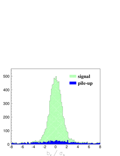
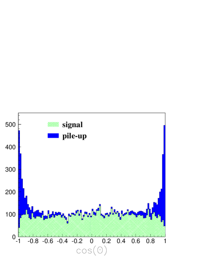
Figure 7: Left: The distribution of the impact parameter $b_{z}$ with respect to the primary vertex divided by its measurement error $\sigma_{b_{z}}$ for signal and pileup tracks. Right: The distribution of the cosine of the polar angle $\theta$ for signal and pileup tracks.

The beamspot length for TESLA is about $300\mu m$, while the measurement error for the impact parameter is only $\approx 5\mu m$. Using the precise measurements from the vertex detector, the primary vertex is first reconstructed as the momentum weighted average z-impact parameter of all tracks in the event.

The difference $b_{z}$ of the z-impact parameter with respect to the primary vertex, divided by the measurement error $\sigma_{b_{z}}$ is shown in Fig. 7 (left) for signal and pileup tracks. Since the distribution for the pileup tracks is much broader than for the signal, only tracks with $|b_{z}|<3\cdot\sigma_{b_{z}}$ are accepted for further event analysis.

The polar angle of each track, i.e. the angle with the beam axis is a further possibility to reduce the pileup. Because of the $t-$channel production mechanism, the pileup tracks are concentrated at low polar angles (Fig. 7, right). Only tracks with a polar angle larger than $18^{\circ}$ (i.e. $|\cos\theta|<0.95$) are kept.

For the reconstruction of jets the standard PYTHIA cluster finding algorithm is used, with the constraint of at least 4 reconstructed jets. The jets are sorted by their transverse momentum $p_{T}$. The low $p_{T}$ jets are very much dominated by pileup tracks, therefore only the 4 jets with the highest $p_{T}$ are taken for the reconstruction of the two $W$-bosons. This is done by combining pairs of jets in such a way that the invariant 2-jet masses $m(W_{1}),m(W_{2})$, i.e. the reconstructed $W$-masses deviate minimally from the on-shell $W$-mass $m_{W}=80.4{\,\mathrm{Ge\kern-1.00006ptV}}$.

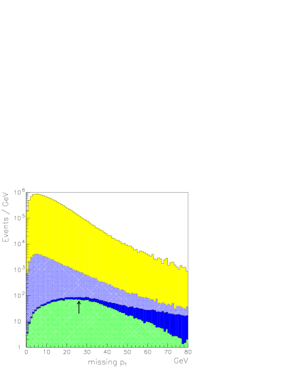
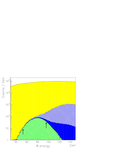
a)	b)
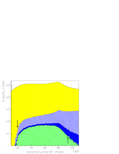
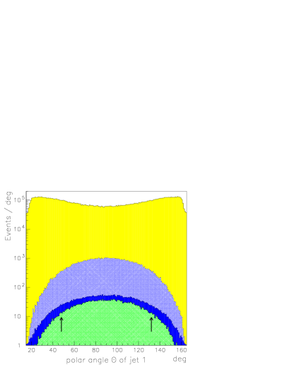
c)	d)

Figure 8: For $\sqrt{s_{ee}}=500{\,\mathrm{Ge\kern-1.00006ptV}}$: a) The missing $p_{T}$ distribution. b) The energy distribution of the reconstructed $W$-boson $W_{1}$. c) The invariant mass of the reconstructed $W_{1}$. d) The polar angle of the jet with highest $p_{T}$. The arrows indicate the applied cuts. The green hatched (light hatched) area represents the signal. The blue (dark) area are the $\gamma\gamma\rightarrow W^{+}W^{-}Z^{0}$ events. The blue hatched (dark hatched) contribution corresponds to $\gamma\gamma\rightarrow t\bar{t}$ events, while the yellow (light) area represents the $\gamma\gamma\rightarrow 4$ jets events.

Observable	$\sqrt{s_{ee}}=500{\,\mathrm{Ge\kern-1.00006ptV}}$		$\sqrt{s_{ee}}=600{\,\mathrm{Ge\kern-1.00006ptV}}$
	min.	max.	min.	max.
acoplanarity	0.225 rad	$\pi$	0.09 rad	$\pi$
missing $p_{T}$	26 GeV	$-$	22 GeV	$-$
thrust	$-$	0.973	$-$	0.983
energy of $W_{1}$	53 GeV	96 GeV	65 GeV	122 GeV
energy of $W_{2}$	50 GeV	99 GeV	58 GeV	124 GeV
lepton - energy	$-$	14 GeV	$-$	20GeV
total energy	132 GeV	226 GeV	110 GeV	262 GeV
reconstructed $W$ - mass	19.5 GeV	94 GeV	23 GeV	116 GeV
visible mass	108 GeV	235 GeV	100 GeV	280 GeV
polar angle of 1st jet	0.84 rad	2.30 rad	0.82 rad	2.32 rad
polar angle of 2nd jet	0.63 rad	2.51 rad	0.58 rad	2.56 rad
polar angle of 3rd jet	0.4 rad	2.74 rad	0.44 rad	2.70 rad
polar angle of 4th jet	0.3 rad	2.84 rad	0.32 rad	2.82 rad
larger polar angle of $W$s	1.35 rad	$\pi$	1.35 rad	$\pi$
smaller polar angle of $W$s	$-$	1.8 rad	$-$	1.85 rad

Table 5: The cut variables that are used in the event analysis for $\sqrt{s_{ee}}=500{\,\mathrm{Ge\kern-1.00006ptV}}$ and $\sqrt{s_{ee}}=600{\,\mathrm{Ge\kern-1.00006ptV}}$. The $min.$/$max.$ values define the range in which the variables have to be so that an event is accepted.

In order to improve the signal to background ratio, cuts were applied on various calculated observables. Table 5 lists all considered variables together with the applied cut condition for the $\sqrt{s_{ee}}=500{\,\mathrm{Ge\kern-1.00006ptV}}$ and $\sqrt{s_{ee}}=600{\,\mathrm{Ge\kern-1.00006ptV}}$ case. Only events that fulfil all cut conditions are accepted and considered as signal-like. The cuts have been optimised by varying the cut conditions one after another and fixing them to the values with best resulting statistical error.

The acoplanarity is defined as $\pi-\delta$, where $\delta$ is the angle between the two reconstructed $W$-bosons in the x-y plane. The distribution of the missing transverse momentum is shown in Fig. 8a for the signal and the three considered backgrounds for $\sqrt{s_{ee}}=500{\,\mathrm{Ge\kern-1.00006ptV}}$. The logarithmic scale illustrates the huge amount of background compared to the signal. Fig. 8b and 8c show distribution of energy and reconstructed mass of $W_{1}$. The cut on the reconstructed W-mass comes out fairly asymmetric around the nominal W-mass because the phase space of the chargino decay favours low mass W-bosons and in addition the usage of only four jets in the analysis, which is needed to reject pileup tracks, biases the reconstruction towards low masses. Further cut variables are the polar angles of the 4 jets that were used for the $W$ reconstruction. Fig. 8d shows the distribution for the jet with highest $p_{T}$. The applied cuts strongly improve the signal to background ratio. Fig. 9 illustrates this for the $\sqrt{s_{ee}}=600{\,\mathrm{Ge\kern-1.00006ptV}}$ case. It shows the energy distribution of a reconstructed $W$ before and after cuts were applied.

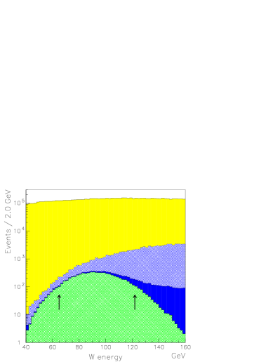
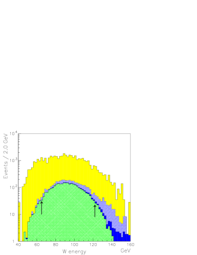
Figure 9: Left: The energy distribution of the reconstructed $W$-boson $W_{1}$ for $\sqrt{s_{ee}}=600{\,\mathrm{Ge\kern-1.00006ptV}}$. Right: The same distribution after applying all cuts except the one on the $W_{1}$-energy. The arrows indicate the cut conditions. The green hatched (light hatched) corresponds to signal, blue (dark) to $\gamma\gamma\rightarrow W^{+}W^{-}Z^{0}$, blue hatched (dark hatched) to $\gamma\gamma\rightarrow t\bar{t}$ and yellow (light) to the $\gamma\gamma\rightarrow 4$ jets events.

Table 6 summarises the cut efficiency, showing the number of events for the signal and the background channels for an integrated luminosity of $1000fb^{-1}$ before and after cuts.

	signal	4 jets	$W^{+}W^{-}Z^{0}$	$t\bar{t}$
${\sqrt{s_{ee}}=500}$ GeV
without cuts	$2620$	$13.7\cdot 10^{6}$	$1565$	$68.8\cdot 10^{3}$
after cuts	453	4065	15	4
${\sqrt{s_{ee}}=600}$ GeV
without cuts	$7976$	$13.4\cdot 10^{6}$	4241	$159.1\cdot 10^{3}$
after cuts	$1925$	$14760$	81	776

Table 6: Number of events per year ($1000fb^{-1}$) for signal and background channels before and after cuts.

7 Results

An efficiency of 17.3% and a purity of 10.0% was obtained for an electron beam centre-of-mass energy of ${\sqrt{s_{ee}}=500{\,\mathrm{Ge\kern-1.00006ptV}}}$, resulting in a statistical error of 14.9% (Table 7). For ${\sqrt{s_{ee}}=600{\,\mathrm{Ge\kern-1.00006ptV}}}$ an efficiency of 24.1% and a purity of 11.0% was obtained, resulting in a statistical error of 6.9%. Because of the higher signal cross section, the statistical error gets smaller for $600{\,\mathrm{Ge\kern-1.00006ptV}}$ compared to $500{\,\mathrm{Ge\kern-1.00006ptV}}$. However, generally the final errors are quite large. This has a couple of reasons: The Standard Model background $\gamma\gamma\rightarrow 4$ jets has a cross section very much larger than the signal. The distinction of signal and background events is more difficult in comparison with the $e^{+}e^{-}$-collider. There is no fixed beam energy that could be used for kinematic constraints (on the $W$-energy for instance). In addition, particles with polar angles below $7^{\circ}$ are not detected, which makes the $p_{T}$ and acoplanarity cuts less effective.

$\mathbf{\sqrt{s_{ee}}}$	signal events per year	background events per year	efficiency $\varepsilon$	purity $p$	stat. error $\Delta N/N$
$500{\,\mathrm{Ge\kern-1.00006ptV}}$	$453$	$4084$	$17.3\%$	$10.0\%$	14.9%
$600{\,\mathrm{Ge\kern-1.00006ptV}}$	$1925$	$15.6\cdot 10^{3}$	$24.1\%$	$11.0\%$	6.9%

Table 7: Number of signal events and the total number of background events after all cuts for $1000fb^{-1}$. In addition the final efficiencies, purities and statistical errors.

Using equation 4 the statistical error for the branching ratio BR(${\tilde{\chi}_{1}^{\pm}}\rightarrow{\tilde{\chi}_{1}^{0}}W^{\pm}$) can be derived. We neglect the error of the luminosity, which is supposed to be on the per mille level. Since the chargino mass will be precisely measured at the Linear Collider, the pair production cross section is known. Therefore, the relative error for BR(${\tilde{\chi}_{1}^{\pm}}\rightarrow{\tilde{\chi}_{1}^{0}}W^{\pm}$) is simply one half of the statistical error ${\Delta N}/{N}$, because the branching ratio enters quadratically in the total cross section.

Thus the result of this analysis is an expected statistical error for the directly measured branching ratio BR(${\tilde{\chi}_{1}^{\pm}}\rightarrow{\tilde{\chi}_{1}^{0}}W^{\pm}$) of 7.5% for ${\sqrt{s_{ee}}=500{\,\mathrm{Ge\kern-1.00006ptV}}}$ and 3.5% for ${\sqrt{s_{ee}}=600{\,\mathrm{Ge\kern-1.00006ptV}}}$.

8 Interpretation with Fittino

In [17] a global fit of the MSSM parameters for the SPS1a scenario has been presented, which was done with the program Fittino [18]. A set of 24 free parameters was fitted, based on a collection of simulated LHC and LC measurements with estimated uncertainties.

We have repeated that fit for the scenario used in this analysis and included the chargino branching ratio with its estimated measurement error as an additional observable. For this purpose the low energy MSSM parameters and observables that correspond to the mSUGRA parameters, which were selected for this analysis, have been calculated with SPHENO [19] first. Table 8 shows the list of all included observables. The estimated measurement errors were taken from [17] and scaled according to the change in the measurement values with respect to those used in the SPS1a fit. The numbers (e.g. the chargino mass $m_{\tilde{\chi}_{1}^{\pm}}$) also differ slightly from the ones that were used as input for the Monte Carlo analysis. Those have been calculated with ISAJET, while Fittino uses SPHENO for the generation of the SUSY particle spectrum.

However, only a subset of parameters has been fitted here for reasons of simplicity. Table 9 shows the parameters that have been fixed to their input values. They concern the squark sector, which is assumed not to be very much influenced by a measurement of the chargino branching ratio.

Measurement	Value	Uncertainty
$m_{\text{h}^{0}}$	110.6 GeV	0.5 GeV
$m_{\text{H}^{0}}$	407.3 GeV	1.3 GeV
$m_{\text{A}^{0}}$	406.6 GeV	1.3 GeV
$m_{\text{H}^{\pm}}$	415.8 GeV	1.1 GeV
$m_{\tilde{\nu}_{\text{e}L}}$	209.2 GeV	0.8 GeV
$m_{\tilde{\text{e}}_{L}}$	223.7 GeV	0.2 GeV
$m_{\tilde{\text{e}}_{R}}$	166.2 GeV	0.06 GeV
$m_{\tilde{\mu}_{L}}$	223.7 GeV	0.5 GeV
$m_{\tilde{\mu}_{R}}$	166.2 GeV	0.2 GeV
$m_{\tilde{\tau}_{1}}$	159.2 GeV	0.4 GeV
$m_{\tilde{\tau}_{2}}$	226.4 GeV	1.2 GeV
$m_{\tilde{\text{g}}}$	600.5 GeV	6.1 GeV
$m_{\tilde{\chi}_{1}^{0}}$	94.86 GeV	0.05 GeV
$m_{\tilde{\chi}_{2}^{0}}$	183.36 GeV	0.08 GeV
$m_{\tilde{\chi}_{1}^{\pm}}$	181.85 GeV	0.55 GeV
$m_{\tilde{\chi}_{2}^{\pm}}$	380.4 GeV	3.0 GeV
$\sigma_{+}$ ( $\text{e}^{+}\text{e}^{-}\rightarrow\tilde{\chi}_{1}^{0}\tilde{\chi}_{2}^{0}$)	20.9 fb	1.8 fb
$\sigma_{+}$ ( $\text{e}^{+}\text{e}^{-}\rightarrow\tilde{\chi}_{2}^{0}\tilde{\chi}_{2}^{0}$)	17.3 fb	1.8 fb
$\sigma_{+}$ ( $\text{e}^{+}\text{e}^{-}\rightarrow\tilde{\text{e}}_{L}\tilde{\text{e}}_{L}$)	156.3 fb	3.0 fb
$\sigma_{+}$ ( $\text{e}^{+}\text{e}^{-}\rightarrow\tilde{\mu}_{L}\tilde{\mu}_{L}$)	27.0 fb	2.9 fb
$\sigma_{+}$ ( $\text{e}^{+}\text{e}^{-}\rightarrow\tilde{\tau}_{1}\tilde{\tau}_{1}$)	28.8 fb	2.9 fb
$\sigma_{+}$ ( $\text{e}^{+}\text{e}^{-}\rightarrow\tilde{\chi}_{1}^{\pm}\tilde{\chi}_{1}^{\mp}$)	43.5 fb	0.9 fb
$\sigma_{+}$ ( $\text{e}^{+}\text{e}^{-}\rightarrow$ Z $\text{h}^{0}$)	11.14 fb	0.21 fb
$\sigma_{-}$ ( $\text{e}^{+}\text{e}^{-}\rightarrow\tilde{\chi}_{1}^{\pm}\tilde{\chi}_{1}^{\mp}$)	97.6 fb	3.3 fb
$\sigma_{-}$ ( $\text{e}^{+}\text{e}^{-}\rightarrow\tilde{\chi}_{1}^{0}\tilde{\chi}_{2}^{0}$)	40.2 fb	1.8 fb
$\sigma_{-}$ ( $\text{e}^{+}\text{e}^{-}\rightarrow\tilde{\chi}_{2}^{0}\tilde{\chi}_{2}^{0}$)	38.8 fb	1.8 fb
$\sigma_{-}$ ( $\text{e}^{+}\text{e}^{-}\rightarrow\tilde{\text{e}}_{L}\tilde{\text{e}}_{L}$)	74.1 fb	3.0 fb
$\sigma_{-}$ ( $\text{e}^{+}\text{e}^{-}\rightarrow\tilde{\text{e}}_{L}\tilde{\text{e}}_{R}$)	169.0 fb	3.0 fb
$\sigma_{-}$ ( $\text{e}^{+}\text{e}^{-}\rightarrow\tilde{\text{e}}_{R}\tilde{\text{e}}_{R}$)	14.4 fb	1.0 fb
$\sigma_{-}$ ( $\text{e}^{+}\text{e}^{-}\rightarrow\tilde{\mu}_{L}\tilde{\mu}_{L}$)	16.6 fb	1.5 fb
$\sigma_{-}$ ( $\text{e}^{+}\text{e}^{-}\rightarrow\tilde{\tau}_{1}\tilde{\tau}_{1}$)	18.8 fb	1.5 fb
BR ( $\text{h}^{0}\rightarrow\text{b}\bar{\text{b}}$ )	0.83	0.01
BR ( $\text{h}^{0}\rightarrow\text{c}\bar{\text{c}}$)	0.04	0.01
BR ( $\text{h}^{0}\rightarrow\tau^{+}\tau^{-}$ )	0.13	0.01

Table 8: The simulated LHC and LC measurements for the considered SUSY scenario. Standard Model parameters and squark masses are not listed. The cross sections correspond to a centre-of-mass energy of $\sqrt{s}=500$ GeV. The electron and positron polarisations are indicated by subscript: “$+$” for $P_{\text{e}^{-}}=0.8$, $P_{\text{e}^{+}}=0.6$ and “$-$” for $P_{\text{e}^{-}}=-0.8$, $P_{\text{e}^{+}}=-0.6$.

Now, three fits have been performed: One, with only the observables from Table 8 without the branching ratio as an included measurement. The second one includes $BR({\tilde{\chi}_{1}^{\pm}}\rightarrow{\tilde{\chi}_{1}^{0}}W^{\pm})=33.4\%$, which is the numerical value obtained with SPHENO, together with a relative measurement error of 7.5% as the result for ${\sqrt{s_{ee}}=500{\,\mathrm{Ge\kern-1.00006ptV}}}$. The third fit is similar but with an error of 3.5% obtained in the as the result for the ${\sqrt{s_{ee}}=600{\,\mathrm{Ge\kern-1.00006ptV}}}$ case. Table 10 shows the fitted parameters and the uncertainties obtained from the three fits. Because we were just interested in the final errors, we simply used the actual input values of the parameters as start values for the fit. In terms of precision, many parameters are not influenced significantly. However the uncertainties on the parameters determining the chargino and neutralino mixing matrices, especially $\tan\beta$, and on $X_{\tau}$ improve, when the branching ratio is added as a measured observable. For $\tan\beta$ the relative error improves by a factor of 2 for ${\Delta BR}/{BR}=3.5\%$. The errors for the stau masses $m_{\tilde{\tau}_{R}}$, $m_{\tilde{\tau}_{L}}$ also get better by roughly a factor of 2. The errors of some other parameters (e.g. $M_{\tilde{e}_{R}}$) might improve a little because of an overall correlation among all fitted parameters. The improper decrease of precision on $\mu$ and $M_{2}$ is due to a slightly unstable fit. It should, however, be noted that up to now no observables sensitive to the decay modes of the superpartners have been studied in $e^{+}e^{-}$.

Parameter	Value (GeV)	Parameter	Value (GeV)	Parameter	Value (GeV)
$X_{t}$	-535.09	$X_{b}$	-3972.09	$M_{3}$	579.42
$m_{\tilde{d}_{R}}$	525.15	$m_{\tilde{s}_{R}}$	525.15	$m_{\tilde{b}_{R}}$	522.65
$m_{\tilde{u}_{R}}$	527.24	$m_{\tilde{c}_{R}}$	527.24	$m_{\tilde{t}_{R}}$	423.98
$m_{\tilde{u}_{L}}$	544.21	$m_{\tilde{c}_{L}}$	544.21	$m_{\tilde{t}_{L}}$	497.43
$m_{t}$	174.3	$m_{b}$	4.2	$m_{c}$	1.2

Table 9: The fixed parameters and their input values.

		uncertainty
Parameter	Value (GeV)	without $BR$	$\frac{\Delta BR}{BR}=7.5\%$	$\frac{\Delta BR}{BR}=3.5\%$
$\tan\beta$	9.00	22%	16%	10%
$X_{\tau}$	-3457.5	19%	7%	6%
$\mu$	355.96	1.2%	1.4%	1.0%
$M_{1}$	99.54	0.3%	0.3%	0.2%
$M_{2}$	192.57	0.4%	0.6%	0.3%
$m_{A_{0}}$	406.59	0.2%	0.2%	0.2%
$M_{\tilde{\tau}_{R}}$	157.31	1.3%	0.5%	0.5%
$M_{\tilde{\tau}_{L}}$	212.28	1.0%	0.6%	0.6%
$M_{\tilde{\mu}_{R}}$	159.41	0.15%	0.15%	0.15%
$M_{\tilde{\mu}_{L}}$	213.04	0.3%	0.3%	0.3%
$M_{\tilde{e}_{R}}$	159.41	0.05%	0.05%	0.04%
$M_{\tilde{e}_{L}}$	213.04	0.10%	0.09%	0.09%

Table 10: The fitted parameters and the uncertainties obtained in the fits. The second column lists the input values.

9 Conclusions

A future photon collider provides the opportunity to measure the branching ratio of the chargino decay ${\tilde{\chi}_{1}^{\pm}}\rightarrow{\tilde{\chi}_{1}^{0}}W^{\pm}$ directly. Considering a mSUGRA scenario similar to SPS1a, this Monte Carlo study showed that a statistical error for the branching ratio of ${\Delta BR}/{BR}=3.5\%$ (7.5%) for an electron centre-of-mass energy of $\sqrt{s}=600$ GeV ($\sqrt{s}=500$ GeV) can be obtained. Such a measurement would improve the precision of a global MSSM parameter fit.

Acknowledgements

We would like to thank the creators of SHERPA especially Frank Krauss, Andreas Schälicke, Steffen Schumann and Tanju Gleisberg for their dedicated help and support. We thank Philip Bechtle and Peter Wienemann for the important assistance in the usage of Fittino. We also thank Hanna Nowak and Sabine Riemann for many helpful discussions.

References

- [1] I. F. Ginzburg, G. L. Kotkin, V. G. Serbo and V. I. Telnov, JETP Lett. 34, 491 (1981).
- [2] B. Badelek et al. [ECFA/DESY Photon Collider Working Group Collaboration], “TESLA Technical Design Report, Part VI, Chapter 1: Photon collider at TESLA,”, arXiv:hep-ex/0108012.
- [3] B. C. Allanach et al., Eur. Phys. J. C25 (2002) 113.
- [4] N. Ghodbane and H. U. Martyn, in Proc. of the APS/DPF/DPB Summer Study on the Future of Particle Physics (Snowmass 2001) ed. N. Graf, arXiv:hep-ph/0201233.
- [5] F. E. Paige, S. D. Protopescu, H. Baer and X. Tata, arXiv:hep-ph/0312045.
- [6] P. Chen, T. Ohgaki, A. Spitkovsky, T. Takahashi and K. Yokoya, Nucl. Instrum. Meth. A 397 (1997) 458 [arXiv:physics/9704012].
- [7] V. Telnov, Nucl. Instrum. Meth. A 472 (2001) 43 [arXiv:hep-ex/0010033].
- [8] T. Mayer, C. Blöchinger, F. Franke and H. Fraas, Eur. Phys. J. C 27 (2003) 135 [arXiv:hep-ph/0209108].
- [9] T. Gleisberg, S. Höche, F. Krauss, A. Schälicke, S. Schumann and J. C. Winter, JHEP 0402 (2004) 056 [arXiv:hep-ph/0311263].
- [10] F. Krauss, R. Kuhn and G. Soff, JHEP 0202 (2002) 044 [arXiv:hep-ph/0109036].
- [11] A. F. Zarnecki, Acta Phys. Polon. B 34 (2003) 2741 [arXiv:hep-ex/0207021].
- [12] M. Pohl and H. J. Schreiber, arXiv:hep-ex/0206009.
- [13] K. Mönig, LC-DET-2004-014 Prepared for International Conference on Linear Colliders (LCWS 04), Paris, France, 19-24 Apr 2004
- [14] A. Schälicke and F. Krauss, arXiv:hep-ph/0503281.
- [15] T. Sjöstrand, L. Lönnblad, S. Mrenna and P. Skands, arXiv:hep-ph/0308153.
- [16] D. Schulte, private communication
- [17] G. Weiglein et al. [LHC/LC Study Group], arXiv:hep-ph/0410364.
- [18] P. Bechtle, K. Desch and P. Wienemann, arXiv:hep-ph/0412012.
- [19] W. Porod, Comput. Phys. Commun. 153 (2003) 275 [arXiv:hep-ph/0301101].