An Introduction to Extra Dimensions

Abstract

Models that involve extra dimensions have introduced completely new ways of looking up on old problems in theoretical physics. The aim of the present notes is to provide a brief introduction to the many uses that extra dimensions have found over the last few years, mainly following an effective field theory point of view. Most parts of the discussion are devoted to models with flat extra dimensions, covering both theoretical and phenomenological aspects. We also discuss some of the new ideas for model building where extra dimensions may play a role, including symmetry breaking by diverse new and old mechanisms. Some interesting applications of these ideas are discussed over the notes, including models for neutrino masses and proton stability. The last part of this review addresses some aspects of warped extra dimensions, and graviton localization.

I Introduction: Why Considering Extra Dimensions?

Possible existence of new spatial dimensions beyond the four we see have been under consideration for about eighty years already. The first ideas date back to the early works of Kaluza and Klein around the 1920’s kk , who tried to unify electromagnetism with Einstein gravity by proposing a theory with a compact fifth dimension, where the photon was originated from the extra components of the metric. In the course of the last few years there has been some considerable activity in the study of models that involve new extra spatial dimensions, mainly motivated from theories that try to incorporate gravity and gauge interactions in a unique scheme in a reliable manner. Extra dimensions are indeed a known fundamental ingredient for String Theory, since all versions of the theory are naturally and consistently formulated only in a space-time of more than four dimensions (actually 10, or 11 if there is M-theory). For some time, however, it was conventional to assume that such extra dimensions were compactified to manifolds of small radii, with sizes about the order of the Planck length, $\ell_{P}\sim~{}10^{-33}$ cm, such that they would remain hidden to the experiment, thus explaining why we see only four dimensions. In this same pictures, it was believed that the relevant energy scale where quantum gravity (and stringy) effects would become important is given by the Planck mass, which is defined through the fundamental constants, including gravity Newton constant, as

$$M_{P}c^{2}=\left[\frac{\hbar c^{5}}{8\pi G_{N}}\right]^{1/2}~{}\sim~{}2.4\times 10^{18}~{}{\rm GeV}~{};$$ (1)

from where one defines $\ell_{P}=\hbar/M_{P}~{}c$. It is common to work in natural units system which take $c=1=\hbar$, such that distance and time are measured in inverse units of energy. We will do so hereafter, unless otherwise stated. Since $M_{P}$ is quite large, there was little hope for experimentally probing such a regime, at least in the near future.

From the theoretical side, this point of view yet posses a fundamental puzzle, related to the quantum instability of the Higgs vacuum that fixes the electroweak scale around $m_{EW}\sim 1~{}TeV$. Problem is that from one loop order corrections, using a cut-off regularization, one gets bare mass independent quadratic divergences for the physical Higgs mass:

$$\delta m_{H}^{2}={1\over 8\pi^{2}}\left(\lambda_{H}-\lambda_{F}^{2}\right)\Lambda^{2}+(\mbox{log. div.})+\mbox{finite terms.}$$ (2)

where $\lambda_{H}$ is the self-couplings of the Higgs field $H$, and $\lambda_{F}$ is the Yukawa coupling to fermions. As the natural cut-off $\Lambda$ of the theory is usually believed to be the Planck scale or the GUT scale, $M_{GUT}\sim 10^{16}~{}GeV$, this means that in order to get $m_{H}^{2}\sim m_{EW}^{2}$ we require to adjust the counterterm to at least one part in $10^{15}$. Moreover, this adjustment must be made at each order in perturbation theory. This large fine tuning is what is known as the hierarchy problem. Of course, the quadratic divergence can be renormalized away in exactly the same manner as it is done for logarithmic divergences, and in principle, there is nothing formally wrong with this fine tuning. In fact, if this calculation is performed in the dimensional regularization scheme, $DR$, one obtains only $1/\epsilon$ singularities which are absorbed into the definitions of the counterterms, as usual. Hence, the problem of quadratic divergences does not become apparent there. It arises only when one attempts to give a physical significance to the cut-off $\Lambda$. In other words, if the SM were a fundamental theory then using $DR$ would be justified. However, most theorists believe that the final theory should also include gravity, then a cut-off must be introduced in the SM, regarding this fine tuning as unattractive. Explaining the hierarchy problem has been a leading motivation to explore new physics during the last twenty years, including Supersymmetry susy and compositeness tech .

Recent developments, based on the studies of the non-perturbative regime of the $E_{8}\times E_{8}$ theory by Witten and Horava witten , have suggested that some, if not all, of the extra dimensions could rather be larger than $\ell_{P}$. Perhaps motivated by this, some authors started to ask the question of how large could these extra dimensions be without getting into conflict with observations, and even more interesting, where and how would this extra dimensions manifest themselves. The intriguing answer to the first question point towards the possibility that extra dimensions as large as millimeters dvali could exist and yet remain hidden to the experiments expt ; giudice ; lykken ; coll1 ; sn87 ; coll2 . This would be possible if our observable world is constrained to live on a four dimensional hypersurface (the brane) embedded in a higher dimensional space (the bulk), such that the extra dimensions can only be tested by gravity, a picture that resembles D-brane theory constructions. Although it is fair to say that similar ideas were already proposed on the 80’s by several authors rubakov , they were missed by some time, until the recent developments on string theory provided an independent realization of such models witten ; anto ; marchesano ; lykk ; dbranes , given them certain credibility. Besides, it was also the intriguing observation that such large extra dimensions would accept a scale of quantum gravity much smaller than $M_{P}$, even closer to $m_{EW}$, thus offering an alternative solution to the hierarchy problem, which attracted the attention of the community towards this ideas.

To answer the second question many phenomenological studies have been done, often based on simplified field theoretical models that are built up on a bottom-up approach, using an effective field theory point of view, with out almost any real string theory calculations. In spite of being quite speculative, and although it is unclear whether any of those models is realized in nature, they still might provide some insights to the low energy manifestations of the fundamental theory, since it is still possible that the excited modes of the string could appear on the experiments way before any quantum gravity effect, in which case the effective field theory approach would be acceptable.

The goal for the present notes is to provide a general and brief introduction to the field for the beginner. Many variants of the very first scenario proposed by Arkani-Hammed, Dimopoulos and D’vali (ADD) dvali have been considered over the years, and there is no way we could comment all. Instead, we shall rather concentrate on some of the most common aspects shared by those models. This, in turn, will provide us with the insight to extend our study to other more elaborated ideas for the use of extra dimensions.

The first part of these notes will cover the basics of the ADD model. We shall start discussing how the fundamental gravity scale departs from $M_{P}$ once extra dimensions are introduced, and the determination of the effective gravity coupling. Then, we will introduce the basic field theory prescriptions used to construct brane models and discuss the concept of dimensional reduction on compact spaces and the resulting Kaluza-Klein (KK) mode expansion of bulk fields, which provide the effective four dimensional theory on which most calculations are actually done. We use these concepts to address some aspects of graviton phenomenology and briefly discuss some of the phenomenological bounds for the size of the extra dimensions and the fundamental gravity scale.

Third section is devoted to present some general aspects of the use of extra dimensions in model building. Here we will review the KK decomposition for matter and gauge fields, and discuss the concept of universal extra dimensions. We will also address the possible phenomenology that may come with KK matter and gauge fields, with particular interest on the power law running effect on gauge couplings. Our fourth section intends to be complementary to the third one. It provides a short review on many new ideas for the use of extra dimensions on the breaking of symmetries. Here we include spontaneous breaking on the bulk; shinning mechanism; orbifold breaking; and Scherk-Schwarz mechanisms.

As it is clear, with a low fundamental scale, as pretended by the ADD model, all the particle physics phenomena that usually invokes high energy scales does not work any more. Then, standard problems as gauge coupling unification, the origin of neutrino masses and mixings and proton decay; should be reviewed. Whereas the first point is being already addressed on the model building section, we dedicate our fifth section to discuss some interesting ideas to control lepton and baryon number violation in the context of extra dimension models. Our discussion includes a series of examples for generating neutrino masses in models with low fundamental scales which make use of bulk fields. We also address proton decay in the context of six dimensional models where orbifold spatial symmetries provide the required control of this process. The concept of fermion wave function localization on the brane is also discussed.

Finally, in section six we focus our interest on Randall and Sundrum models merab ; rs1 ; rs2 ; nimars for warped backgrounds, for both compact and infinite extra dimensions. We will show in detail how these solutions arise, as well as how gravity behaves in such theories. Some further ideas that include stabilization of the extra dimensions and graviton localization at branes are also covered.

Due to the nature of these notes, many other topics are not being covered, including brane intersecting models, cosmology of models with extra dimensions both in flat and warped bulk backgrounds; KK dark matter; an extended discussion on black hole physics; as well as many others. The interested reader that would like to go beyond the present notes can consult any of the excellent reviews that are now in the literature for references, some of which are given in references reviews ; review1 . Further references are also given at the conclusions.

II Flat and Compact Extra Dimensions: ADD Model

II.1 Fundamental vs. Planck scales

The existence of more than four dimensions in nature, even if they were small, may not be completely harmless. They could have some visible manifestations in our (now effective) four dimensional world. To see this, one has first to understand how the effective four dimensional theory arises from the higher dimensional one. Formally, this can be achieve by dimensionally reducing the complete theory, a concept that we shall further discuss later on. For the moment, we must remember that gravity is a geometric property of the space. Then, first thing to notice is that in a higher dimensional world, where Einstein gravity is assumed to hold, the gravitational coupling does not necessarily coincide with the well known Newton constant $G_{N}$, which is, nevertheless, the gravity coupling we do observe. To explain this more clearly, let us assume as in Ref. dvali that there are $n$ extra space-like dimension which are compactified into circles of the same radius R (so the space is factorized as a ${\cal M}_{4}\times T^{n}$ manifold). We will call the fundamental gravity coupling $G_{\ast}$, and then write down the higher dimensional gravity action:

$$S_{grav}=-\frac{1}{16\pi G_{\ast}}\int\!d^{4+n}x~{}\sqrt{|g_{(4+n)}|}~{}R_{(4+n)}~{};$$ (3)

where $g_{(4+n)}$ stands for the metric in the whole $(4+n)$D space, $ds^{2}=g_{MN}dx^{M}dx^{N}$, for which we will always use the $(+,-,-,-,\dots)$ sign convention, and $M,N=0,1,\dots,n+3$. The above action has to have proper dimensions, meaning that the extra length dimensions that come from the extra volume integration have to be equilibrated by the dimensions on the gravity coupling. Notice that in natural units $S$ has no dimensions, whereas if we assume for simplicity that the metric $g_{(4+n)}$ is being taken dimensionless, so $[R_{(4+n)}]=[Length]^{-2}=[Energy]^{2}$. Thus, the fundamental gravity coupling has to have dimensions $[G_{\ast}]=[Energy]^{-(n+2)}$. In contrast, for the Newton constant, we have $[G_{N}]=[Energy]^{-2}$. In order to extract the four dimensional gravity action let us assume that the extra dimensions are flat, thus, the metric has the form

$$ds^{2}=g_{\mu\nu}(x)dx^{\mu}dx^{\nu}-\delta_{ab}dy^{a}dy^{b},$$ (4)

where $g_{\mu\nu}$ gives the four dimensional part of the metric which depends only in the four dimensional coordinates $x^{\mu}$, for $\mu=0,1,2,3$; and $\delta_{ab}dy^{a}dy^{b}$ gives the line element on the bulk, whose coordinates are parameterized by $y^{a}$, $a=1,\dots,n$. It is now easy to see that $\sqrt{|g_{(4+n)}|}=\sqrt{|g_{(4)}|}$ and $R_{(4+n)}=R_{(4)}$, so one can integrate out the extra dimensions in Eq. (3) to get the effective 4D action

$$S_{grav}=-\frac{V_{n}}{16\pi G_{\ast}}\int\!d^{4}x~{}\sqrt{|g_{(4)}|}~{}R_{(4)}~{};$$ (5)

where $V_{n}$ stands for the volume of the extra space. For the torus we simply take $V_{n}=R^{n}$. Equation (5) is precisely the standard gravity action in 4D if one makes the identification,

$$G_{N}=G_{\ast}/V_{n}~{}.$$ (6)

Newton constant is therefore given by a volumetric scaling of the truly fundamental gravity scale. Thus, $G_{N}$ is in fact an effective quantity. Notice that even if $G_{\ast}$ were a large coupling (as an absolute number), one can still understand the smallness of $G_{N}$ via the volumetric suppression.

To get a more physical meaning of these observations, let us consider a simple experiment. Let us assume a couple of particles of masses $m_{1}$ and $m_{2}$, respectively, located on the hypersurface $y^{a}=0$, and separated from each other by a distance $r$. The gravitational flux among both particles would spread all over the whole $(4+n)$ D space, however, since the extra dimensions are compact, the effective strength of the gravity interaction would have two clear limits: (i) If both test particles are separated from each other by a distance $r\gg R$, the torus would effectively disappear for the four dimensional observer, the gravitational flux then gets diluted by the extra volume and the observer would see the usual (weak) 4D gravitational potential

$$U_{N}(r)=-G_{N}\frac{m_{1}m_{2}}{r}~{}.$$ (7)

(ii) However, if $r\ll R$, the 4D observer would be able to feel the presence of the bulk through the flux that goes into the extra space, and thus, the potential between each particle would appear to be stronger:

$$U_{\ast}(r)=-G_{\ast}\frac{m_{1}m_{2}}{r^{n+1}}~{}.$$ (8)

It is precisely the volumetric factor which does the matching of both regimes of the theory. The change in the short distance behavior of the Newton’s gravity law should be observable in the experiments when measuring $U(r)$ for distances below $R$. Current search for such deviations has gone down to 160 microns, so far with no signals of extra dimensions expt .

We should now recall that the Planck scale, $M_{P}$, is defined in terms of the Newton constant, via Eq. (1). In the present picture, it is then clear that $M_{P}$ is not fundamental anymore. The true scale for quantum gravity should rather be given in terms of $G_{\ast}$ instead. So, we define the fundamental (string) scale as

$$M_{\ast}c^{2}=\left[\frac{\hbar^{1+n}c^{5+n}}{8\pi G_{\ast}}\right]^{1/(2+n)}~{},$$ (9)

where, for comparing to Eq. (1), we have inserted back the corresponding $c$ and $\hbar$ factors. Clearly, coming back to natural units, both scales are then related to each other by dvali

$$M_{P}^{2}=M_{\ast}^{n+2}V_{n}~{}.$$ (10)

From particle physics we already know that there is no evidence of quantum gravity (neither supersymmetry, nor string effects) well up to energies around few hundred GeV, which says that $M_{\ast}\geq 1$ TeV. If the volume were large enough, then the fundamental scale could be as low as the electroweak scale, and there would be no hierarchy in the fundamental scales of physics, which so far has been considered as a puzzle. Of course, the price of solving the hierarchy problem this way would be now to explain why the extra dimensions are so large. Using $V\sim R^{n}$ one can reverse above relation and get a feeling of the possible values of $R$ for a given $M_{\ast}$. This is done just for our desire of having the quantum gravity scale as low as possible, perhaps to be accessible to future experiments, although, the actual value is really unknown. As an example, if one takes $M_{\ast}$ to be 1 TeV; for $n=1$, $R$ turns out to be about the size of the solar system ($R\sim 10^{11}$ m)!, whereas for $n=2$ one gets $R\sim 0.2$ mm, that is just at the current limit of short distance gravity experiments expt . Of course, one single large extra dimension is not totally ruled out. Indeed, if one imposes the condition that $R<160\mu m$ for $n=1$, we get $M_{\ast}>10^{8}GeV$. More than two extra dimensions are in fact expected (string theory predicts six more), but in the final theory those dimensions may turn out to have different sizes, or even geometries. More complex scenarios with a hierarchical distributions of the sizes could be possible. For getting an insight of the theory, however, one usually relies in toy models with a single compact extra dimension, implicitly assuming that the effects of the other compact dimensions do decouple from the effective theory.

It is worth mentioning that the actual relationship among fundamental, Planck, and compactification scales does depend on the type of metric one assumes for the compact space (although this should be com-formally flat at least). This has inspired some variants on the above simple picture. We will treat in some detail one specific example in the last part of these notes, the Randall-Sundrum models. There is also another nice example I would like to mention where $M_{*}R$ is rather of order one. This is possible if extra dimensions are compactified on a hyperbolic manifold, where the volume is exponentially amplified from the curvature radius, which goes as $Re^{a}$, with the constant $a$ depending on the pattern of compactification hipered . In these models it is possible to get large volumes with generic values of $R$ by properly choosing the parameter $a$. In what follows, however, we will address only ADD models for simplicity.

II.2 Brane and Bulk Effective Field Theory prescriptions

While submillimeter dimensions remain untested for gravity, the particle physics forces have certainly been accurately measured up to weak scale distances (about $10^{-18}$ cm). Therefore, the Standard Model (SM) particles can not freely propagate in those large extra dimensions, but must be constrained to live on a four dimensional submanifold. Then the scenario we have in mind is one where we live in a four dimensional surface embedded in a higher dimensional space. Such a surface shall be called a “brane” (a short name for membrane). This picture is similar to the D-brane models dbranes , as in the Horava-Witten theory witten . We may also imagine our world as a domain wall of size $M_{\ast}^{-1}$ where the particle fields are trapped by some dynamical mechanism dvali . Such hypersurface or brane would then be located at an specific point on the extra space, usually, at the fixed points of the compact manifold. Clearly, such picture breaks translational invariance, which may be reflected in two ways in the physics of the model, affecting the flatness of the extra space (which compensates for the required flatness of the brane), and introducing a source of violation of the extra linear momentum. First point would drive us to the Randall-Sundrum Models, that we shall discuss latter on. Second point would be a constant issue along our discussions.

What we have called a brane in our previous paragraph is actually an effective theory description. We have chosen to think up on them as topological defects (domain walls) of almost zero width, which could have fields localized to its surface. String theory D-branes (Dirichlet branes) are, however, surfaces where open string can end on. Open strings give rise to all kinds of fields localized to the brane, including gauge fields. In the supergravity approximation these D-branes will also appear as solitons of the supergravity equations of motion. In our approach we shall care little about where these branes come from, and rather simply assume there is some consistent high-energy theory, that would give rise to these objects, and which should appear at the fundamental scale $M_{\ast}$. Thus, the natural UV cutoff of our models would always be given by the quantum gravity scale.

D-branes are usually characterized by the number of spatial dimensions on the surface. Hence, a $p$-brane is described by a flat space time with $p$ space-like and one time-like coordinates. The simplest model, we just mentioned above , would consist of SM particles living on a 3-brane. Thus, we need to describe theories that live either on the brane (as the Standard Model) or in the bulk (like gravity and perhaps SM singlets), as well as the interactions among these two theories. For doing so we use the following field theory prescriptions:

• Bulk theories are described by the higher dimensional action, defined in terms of a Lagrangian density of bulk fields, $\phi(x,\vec{y})$, valued on all the space-time coordinates of the bulk

  $$S_{\rm bulk}[\phi]=\int\!d^{4}x\,d^{n}y~{}\sqrt{|g_{(4+n)}|}{\cal L}(\phi(x,\vec{y}))~{},$$ (11)

  where, as before, $x$ stands for the (3+1) coordinates of the brane and $y$ for the $n$ extra dimensions.

• Brane theories are described by the (3+1)D action of the brane fields, $\varphi(x)$, which is naturally promoted into a higher dimensional expression by the use of a delta density:

  $$S_{\rm brane}[\varphi]=\int\!d^{4}x\,d^{n}y~{}\sqrt{|g_{(4)}|}{\cal L}(\varphi(x))~{}\delta^{n}({\vec{y}}-{\vec{y}}_{0})~{},$$ (12)

  where we have taken the brane to be located at the position ${\vec{y}}={\vec{y}}_{0}$ along the extra dimensions, and $g_{(4)}$ stands for the (3+1)D induced metric on the brane. Usually we will work on flat space-times, unless otherwise stated.

• Finally, the action may contain terms that couple bulk to brane fields. Last are localized on the space, thus, it is natural that a delta density would be involved in such terms, say for instance

  $$\int\!d^{4}x\,d^{n}y~{}\sqrt{|g_{(4)}|}~{}\phi(x,\vec{y})\,\bar{\psi}(x)\psi(x)~{}\delta^{n}({\vec{y}}-{\vec{y}}_{0})$$ (13)

II.3 Dimensional Reduction

The presence of delta functions in the previous action terms does not allow for a transparent interpretation, nor for an easy reading out of the theory dynamics. When they are present it is more useful to work in the effective four dimensional theory that is obtained after integrating over the extra dimensions. This procedure is generically called dimensional reduction. It also helps to identify the low energy limit of the theory (where the extra dimensions are not visible).

A 5D toy model.- To get an insight of what the effective 4D theory looks like, let us consider a simplified five dimensional toy model where the fifth dimension has been compactified on a circle of radius $R$. The generalization of these results to more dimensions would be straightforward. Let $\phi$ be a bulk scalar field for which the action on flat space-time has the form

$$S[\phi]=\frac{1}{2}\int\!d^{4}x\ dy\ \left(\partial^{A}\phi\partial_{A}\phi-m^{2}\phi^{2}\right);$$ (14)

where now $A=1,\dots,5$, and $y$ denotes the fifth dimension. The compactness of the internal manifold is reflected in the periodicity of the field, $\phi(y)=\phi(y+2\pi R)$, which allows for a Fourier expansion as

$$\phi(x,y)=\frac{1}{\sqrt{2\pi R}}\phi_{0}(x)+\sum_{n=1}^{\infty}\frac{1}{\sqrt{\pi R}}\left[\phi_{n}(x)\cos\left(\frac{ny}{R}\right)+\hat{\phi}_{n}(x)\sin\left(\frac{ny}{R}\right)\right].$$ (15)

The very first term, $\phi_{0}$, with no dependence on the fifth dimension is usually referred as the zero mode. Other Fourier modes, $\phi_{n}$ and $\hat{\phi}_{n}$; are called the excited or Kaluza-Klein (KK) modes. Notice the different normalization on all the excited modes, with respect to the zero mode. Some authors prefer to use a complex $e^{iny/R}$ Fourier expansion instead, but the equivalence of the procedure should be clear.

By introducing last expansion into the action (14) and integrating over the extra dimension one gets

$$S[\phi]=\sum_{n=0}^{\infty}\frac{1}{2}\int\!d^{4}x\left(\partial^{\mu}\phi_{n}\partial_{\mu}\phi_{n}-m_{n}^{2}\phi_{n}^{2}\right)+\sum_{n=1}^{\infty}\frac{1}{2}\int\!d^{4}x\left(\partial^{\mu}\hat{\phi}_{n}\partial_{\mu}\hat{\phi}_{n}-m_{n}^{2}\hat{\phi}_{n}^{2}\right),$$ (16)

where the KK mass is given as $m_{n}^{2}=m^{2}+\frac{n^{2}}{R^{2}}$. Therefore, in the effective theory, the higher dimensional field appears as an infinite tower of fields with masses $m_{n}$, with degenerated massive levels, but the zero mode, as depicted in figure 1. Notice that all excited modes are fields with the same spin, and quantum numbers as $\phi$. They differ only in the KK number $n$, which is also associated with the fifth component of the momentum, which is discrete due to compatification. This can be also understood in general from the higher dimensional invariant $p^{A}p_{A}=m^{2}$, which can be rewritten as the effective four dimensional squared momentum invariant $p^{\mu}p_{\mu}=m^{2}+{{\vec{p}}_{\bot}}\,^{2}$, where ${\vec{p}}_{\bot}$ stands for the extra momentum components.

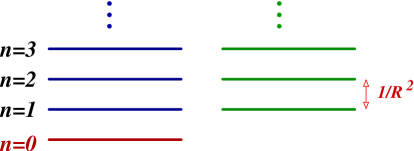
Figure 1: KK mass spectrum for a field on the circle.

Dimensionally reducing any higher dimensional field theory (on the torus) would give a similar spectrum for each particle with larger level degeneracy ($2^{n}$ states per KK level). Different compactifications would lead to different mode expansions. Eq. (15) would had to be chosen accordingly to the geometry of the extra space by typically using wave functions for free particles on such a space as the basis for the expansion. Extra boundary conditions associated to specific topological properties of the compact space may also help for a proper selection of the basis. A useful example is the one dimensional orbifold, $U(1)/Z_{2}$, which is built out of the circle, by identifying the opposite points around zero, so reducing the physical interval of the original circle to $[0,\pi]$ only. Operatively, this is done by requiring the theory to be invariant under the extra parity symmetry $Z_{2}:y\rightarrow-y$. Under this symmetries all fields should pick up a specific parity, such that $\phi(-y)=\pm\phi(y)$. Even (odd) fields would then be expanded only into cosine (sine) modes, thus, the KK spectrum would have only half of the modes (either the left or the right tower in figure 1). Clearly, odd fields do not have zero modes and thus do not appear at the low energy theory.

For $m=0$, it is clear that for energies below $\frac{1}{R}$ only the massless zero mode will be kinematically accessible, making the theory looking four dimensional. The appreciation of the impact of KK excitations thus depends on the relevant energy of the experiment, and on the compactification scale $\frac{1}{R}$:

• For energies $E\ll\frac{1}{R}$ physics would behave purely as four dimensional.

• At larger energies, $\frac{1}{R}<E<M_{\ast}$, or equivalently as we do measurements at shorter distances, a large number of KK excitations, $\sim(ER)^{n}$, becomes kinematically accessible, and their contributions relevant for the physics. Therefore, right above the threshold of the first excited level, the manifestation of the KK modes will start evidencing the higher dimensional nature of the theory.

• At energies above $M_{\ast}$, however, our effective approach has to be replaced by the use of the fundamental theory that describes quantum gravity phenomena.

Coupling suppressions.- Notice that the five dimensional scalar field $\phi$ we just considered has mass dimension $\frac{3}{2}$, in natural units. This can be easily seeing from the kinetic part of the Lagrangian, which involves two partial derivatives with mass dimension one each, and the fact that the action is dimensionless. In contrast, by similar arguments, all excited modes have mass dimension one, which is consistent with the KK expansion (15). In general for $n$ extra dimensions we get the mass dimension for an arbitrary field to be $[\phi]=d_{4}+\frac{n}{2}$, where $d_{4}$ is the natural mass dimension of $\phi$ in four dimensions.

Because this change on the dimensionality of $\phi$, most interaction terms on the Lagrangian (apart from the mass term) would all have dimensionful couplings. To keep them dimensionless a mass parameter should be introduced to correct the dimensions. It is common to use as the natural choice for this parameter the cut-off of the theory, $M_{\ast}$. For instance, let us consider the quartic couplings of $\phi$ in 5D. Since all potential terms should be of dimension five, we should write down $\frac{\lambda}{M_{\ast}}\phi^{4}$, with $\lambda$ dimensionless. After integrating the fifth dimension, this operator will generate quartic couplings among all KK modes. Four normalization factors containing $1/\sqrt{R}$ appear in the expansion of $\phi^{4}$. Two of them will be removed by the integration, thus, we are left with the effective coupling $\lambda/MR$. By introducing Eq. (10) we observe that the effective couplings have the form

$$\lambda\left(\frac{M_{\ast}}{M_{P}}\right)^{2}\phi_{k}\phi_{l}\phi_{m}\phi_{k+l+m}~{};$$ (17)

where the indices are arranged to respect the conservation of the fifth momentum. From the last expression we conclude that in the low energy theory ($E<M_{\ast}$), even at the zero mode level, the effective coupling appears suppressed respect to the bulk theory. Therefore, the effective four dimensional theory would be weaker interacting compared to the bulk theory. Let us recall that same happens to gravity on the bulk, where the coupling constant is stronger than the effective 4D coupling, due to the volume suppression given in Eq. (6), or equivalently in Eq. (10).

Similar arguments apply in general for brane-bulk couplings. Let us, for instance, consider the case of a brane fermion, $\psi(x)$, coupled to our bulk scalar $\phi$ field. For simplicity we assume that the brane is located at the position $y_{0}=0$, which in the case of orbifolds corresponds to a fixed point. Thus, as the part of the action that describes the brane-bulk coupling we choose the term

$$\int\!d^{4}x\ dy\ \frac{h}{\sqrt{M_{\ast}}}\bar{\psi}(x)\psi(x)\phi(x,y=0)\ \delta(y)=\int\!d^{4}x\frac{M_{\ast}}{M_{P}}h\cdot\bar{\psi}\psi\left(\phi_{0}+\sqrt{2}\sum_{n=1}^{\infty}\phi_{n}\right).$$ (18)

Here the Yukawa coupling constant $h$ is dimensionless and the suppression factor $1/\sqrt{M}$ has been introduce to correct the dimensions. On the right hand side we have used the expansion (15) and Eq. (10). From here, we notice that the coupling of brane to bulk fields is generically suppressed by the ratio $M\over M_{P}$. Also, notice that the modes $\hat{\phi}_{n}$ decouple from the brane. Through this coupling we could not distinguish the circle from the orbifold compactification.

Let us stress that the couplings in Eq. (18) do not conserve the KK number. This reflects the fact that the brane breaks the translational symmetry along the extra dimension. Nevertheless, it is worth noticing that the four dimensional theory is still Lorentz invariant. Thus, if we reach enough energy on the brane, on a collision for instance, as to produce real emission of KK modes, part of the energy of the brane would be released into the bulk. This would be the case of gravity, since the graviton is naturally a field that lives in all dimensions.

Next, let us consider the scattering process among brane fermions $\psi\psi\rightarrow\psi\psi$ mediated by all the KK excitations of some field $\phi$. A typical amplitude will receive the contribution

$${\cal M}=\hat{h}^{2}\left(\frac{1}{q^{2}-m^{2}}+2\sum_{n=1}\frac{1}{q^{2}-m_{n}^{2}}\right)D(q^{2}),$$ (19)

where $\hat{h}=(M_{\ast}/M_{P})h$ represents the effective coupling, and $D(q^{2})$ is an operator that only depends on the 4D Feynman rules of the involved fields. The sum can easily be performed in this simple case, and one gets

$${\cal M}=\frac{\hat{h}^{2}\pi R}{\sqrt{q^{2}-m^{2}}}\cot\left[\pi R\sqrt{q^{2}-m^{2}}\right]D(q^{2}).$$ (20)

In more than five dimensions the equivalent to the above sum usually diverges and has to be regularized by introducing a cut-off at the fundamental scale.

We can also consider some simple limits to get a better feeling on the KK contribution to the process. At low energies, for instance, by assuming that $q^{2}\ll m^{2}\ll 1/R^{2}$ we may integrate out all the KK excitations, and at the first order we get the amplitude

$${\cal M}\approx{\hat{h}^{2}\over m^{2}}\left(1+{\pi^{2}\over 3}m^{2}R^{2}\right)D(q^{2}).$$ (21)

Last term between parenthesis is a typical effective correction produced by the KK modes exchange to the pure four dimensional result.

On the other hand, at high energies, $qR\gg 1$, the overall factor becomes $\hat{h}^{2}N$, where $N=MR=M_{P}^{2}/M_{\ast}^{2}$ is the number of KK modes up to the cut-off. This large number of modes would overcome the suppression in the effective coupling, such that one gets the amplitude ${\cal M}\approx h^{2}D(q^{2})/q^{2}$, evidencing the 5D nature of the theory, where there is actually just a single higher dimensional field being exchange but with a larger coupling.

II.4 Graviton Phenomenology and Some Bounds

II.4.1 Graviton couplings and the effective gravity interaction law.

One of the first physical examples of a brane-bulk interaction one may be interested in analyzing with some care is the effective gravitational coupling of particles located at the brane, for which one needs to understand the way gravitons couple to brane fields. The problem has been extendedly discussed by Giudice, Ratazzi and Wells giudice and independently by Han, Lykken and Zhang lykken assuming a flat bulk. Here we summarize some of the main points. We start from the action that describes a particle on the brane

$$S=\int\!d^{4}xd^{n}y\,\sqrt{|g(y^{a}=0)|}~{}{\cal L}~{}\delta^{(n)}(y)~{},$$ (22)

where the induced metric $g(y^{a}=0)$ now includes small metric fluctuations $h_{MN}$ over flat space, which are also called the graviton, such that

$$g_{MN}=\eta_{MN}+\frac{1}{2M_{\ast}^{n/2+1}}h_{MN}.$$ (23)

The source of those fluctuations are of course the energy on the brane, i.e., the matter energy momentum tensor $\sqrt{g}~{}T^{\mu\nu}=\delta S/\delta g_{\mu\nu}$ that enters on the RHS of Einstein equations:

$$R_{MN}-\frac{1}{2}R_{(4+n)}g_{MN}=-\frac{1}{M_{\ast}^{2+n}}T_{\mu\nu}\eta^{\mu}_{M}\eta^{\nu}_{N}\delta^{(n)}(y)~{}.$$

The effective coupling, at first order in $h$, of matter to graviton field is then described by the action

$$S_{int}=\int\!d^{4}x\frac{h_{\mu\nu}}{M_{\ast}^{n/2+1}}T^{\mu\nu}$$ (24)

It is clear from the effective four dimensional point of view, that the fluctuations $h_{MN}$ would have different 4D Lorentz components. (i) $h_{\mu\nu}$ clearly contains a 4D Lorentz tensor, the true four dimensional graviton. (ii) $h_{a\mu}$ behaves as a vector, the graviphotons. (iii) Finally, $h_{ab}$ behaves as a group of scalars (graviscalar fields), one of which corresponds to the partial trace of $h$ (${h^{a}}_{a}$) that we will call the radion field. To count the number of degrees of freedom in $h_{MN}$ we should first note that $h$ is a $D\times D$ symmetric tensor, for $D=4+n$. Next, general coordinate invariance of general relativity can be translated into $2n$ independent gauge fixing conditions, half usually chosen as the harmonic gauge $\partial_{M}h_{N}^{M}=\frac{1}{2}\partial_{N}h^{M}_{M}$. In total there are $n(n-3)/2$ independent degrees of freedom. Clearly, for $n=4$ one has the usual two helicity states of a massless spin two particle.

All those effective fields would of course have a KK decomposition,

$$h_{MN}(x,y)=\sum_{\vec{n}}\frac{h_{MN}^{(\vec{n})}(x)}{\sqrt{V_{n}}}~{}e^{i\vec{n}\cdot\vec{y}/R}~{},$$ (25)

where we have assumed the compact space to be a torus of unique radius $R$, also here $\vec{n}=(n_{1},\dots,n_{n})$, with all $n_{a}$ integer numbers. Once we insert back the above expansion into $S_{int}$, it is not hard to see that the volume suppression will exchange the $M_{\ast}^{n/2+1}$ by an $M_{P}$ suppression for the the effective interaction with a single KK mode. Therefore, all modes couple with standard gravity strength. Briefly, only the 4D gravitons, $G_{\mu\nu}$, and the radion field, $b(x)$, get couple at first order level to the brane energy momentum tensor giudice ; lykken

$${\cal L}=-\frac{1}{M_{P}}\sum_{\vec{n}}\left[G^{(\vec{n})\mu\nu}-\frac{1}{3}\sqrt{\frac{2}{3(n+2)}}b^{(\vec{n})}\eta^{\mu\nu}\right]T_{\mu\nu}.$$ (26)

Notice that $G^{(0)\mu\nu}$ is massless since the higher dimensional graviton $h_{MN}$ has no mass itself. That is the source of long range four dimensional gravity interactions. It is worth saying that on the contrary $b^{(0)}$ should not be massless, otherwise it should violate the equivalence principle, since it would mean a scalar (gravitational) interaction of long range too. $b^{(0)}$ should get a mass from the stabilization mechanism that keeps the extra volume finite.

Now that we know how gravitons couple to brane matter we can use this effective field theory point of view to calculate what the effective gravitational interaction law should be on the brane. KK gravitons are massive, thus, the interaction mediated by them on the brane is of short range. More precisely, each KK mode contribute to the gravitational potential among two test particles of masses $m_{1}$ and $m_{2}$ located on the brane, separated by a distance $r$, with a Yukawa potential

$$\Delta_{\vec{n}}U(r)\simeq-G_{N}\frac{m_{1}m_{2}}{r}e^{-m_{\vec{n}}r}=U_{N}(r)e^{-m_{\vec{n}}r}~{}.$$ (27)

Total contribution of all KK modes, the sum over all KK masses $m_{\vec{n}}^{2}=\vec{n}^{2}/R$, can be estimated in the continuum limit, to get

$$U_{T}(r)\simeq-G_{N}V_{n}(n-1)!~{}\frac{m_{1}m_{2}}{r^{n+1}}\simeq U_{\ast}(r)~{},$$ (28)

as mentioned in Eq. (8). Experimentally, however, for $r$ just around the threshold $R$ only the very first excited modes would be relevant, and so, the potential one should see in short distance tests of Newton’s law should rather be of the form sfetsos

$$U(r)\simeq U_{N}(r)\left(1+\alpha e^{-r/R}\right)~{}.$$ (29)

where $\alpha=8n/3$ accounts for the multiplicity of the very first excited level. As already mentioned, recent measurements have tested inverse squared law of gravity down to about 160 $\mu m$, and no signals of deviation have been found expt .

II.4.2 Collider physics.

As gravity may become comparable in strength to the gauge interactions at energies $M\ast\sim$ TeV, the nature of the quantum theory of gravity would become accessible to LHC and NLC. Indeed, the effect of the gravitational couplings would be mostly of two types: (i) missing energy, that goes into the bulk; and (ii) corrections to the standard cross sections from graviton exchange coll1 . A long number of studies on this topics have appeared giudice ; lykken ; coll1 , and some nice and short reviews of collider signatures were early given in review1 . Here we just briefly summarize some of the possible signals. Some indicative bounds one can obtain from the experiments on the fundamental scale are also shown in tables 1 and 2. Notice however that precise numbers do depend on the number of extra dimensions. At $e^{+}e^{-}$ colliders (LEP,LEPII, L3), the best signals would be the production of gravitons with $Z,\gamma$ or fermion pairs $\bar{f}f$. In hadron colliders (CDF, LHC) one could see graviton production in Drell-Yang processes, and there is also the interesting monojet production giudice ; lykken which is yet untested. LHC could actually impose bounds up to 4 TeV for $M_{\ast}$ for 10 $fb^{-1}$ luminosity.

Graviton exchange either leads to modifications of the SM cross sections and asymmetries, or to new processes not allowed in the SM at tree level. The amplitude for exchange of the entire tower naively diverges when $n>1$ and has to be regularized, as already mentioned. An interesting channel is $\gamma\gamma$ scattering, which appears at tree level, and may surpasses the SM background at $s=0.5$ TeV for $M_{\ast}=4$ TeV. Bi-boson productions of $\gamma\gamma$, $WW$ and $ZZ$ may also give some competitive bounds giudice ; lykken ; coll1 . Some experimental limits, most of them based on existing data, are given in Table 2. The upcoming experiments will easily overpass those limits.

Table 1: Collider limits for the fundamental scale $M_{\ast}$. Graviton Production.

Process	Background	$M_{\ast}$ limit	Collider
$e^{+}e^{-}\rightarrow\gamma G$	$e^{+}e^{-}\rightarrow\gamma\bar{\nu}\nu$	1 TeV	L3
$e^{+}e^{-}\rightarrow ZG$	$e^{+}e^{-}\rightarrow Z\bar{\nu}\nu$	$\bigg{\{}\begin{array}[]{l}515~{}GeV\\ 600~{}GeV\end{array}$	$\begin{array}[]{l}\mbox{LEPII}\\ \mbox{L3}\end{array}$
$Z\rightarrow\bar{f}fG$	$Z\rightarrow\bar{f}f\bar{\nu}\nu$	0.4 TeV	LEP

Table 2: Collider limits for the fundamental scale $M_{\ast}$. Virtual Graviton exchange

Process	$M_{\ast}$ limit	Collider
$e^{+}e^{-}\rightarrow f\bar{f}$	0.94 TeV	Tevatron & HERA
$e^{+}e^{-}\rightarrow\gamma\gamma,WW,ZZ$	$\bigg{\{}\begin{array}[]{l}0.7--1~{}TeV\\ 0.8~{}TeV\end{array}$	$\begin{array}[]{l}\mbox{LEP}\\ \mbox{L3}\end{array}$
All above	1 TeV	L3
Bhabha scattering	1.4 TeV	LEP
$\begin{array}[]{l}q\bar{q}\rightarrow\gamma\gamma\\ gg\rightarrow\gamma\gamma\end{array}\bigg{\}}$	0.9 TeV	CDF

Another intriguing phenomena in colliders, associated to a low gravity scale, is the possible production of microscopic Black Holes bh1 . Given that the $(4+n)D$ Schwarzschild radius

$$r_{S}\sim\left(\frac{M_{BH}}{M_{\ast}}\right)^{\frac{1}{1+n}}\frac{1}{M_{\ast}}$$ (30)

may be larger than the impact parameter in a collision at energies larger than $M_{\ast}$, it has been conjecture that a Black Hole may form with a mass $M_{BH}=\sqrt{s}$. Since the geometrical cross section of the Black Hole goes as $\sigma\sim\pi r_{S}^{2}~{}~{}\sim TeV^{-2}\approx 400~{}pb$, it has been pointed out that LHC running at maximal energy could even be producing about $10^{7}$ of those Black Holes per year, if $M_{\ast}\sim TeV$. However, such tiny objects are quite unstable. Indeed they thermally evaporate in a life time

$$\tau\approx\frac{1}{M_{\ast}}\left(\frac{M_{BH}}{M_{\ast}}\right)^{(3n+1)/(n+1)}$$ (31)

by releasing all its energy into Hawking radiation containing predominantly brane modes. For above parameters one gets $\tau<10^{-25}~{}sec$. This efficient conversion of collider energy into thermal radiation would be a clear signature of having reached the quantum gravity regime.

II.4.3 Cosmology and Astrophysics.

Graviton production may also posses strong constraints on the theory when considering that the early Universe was an important resource of energy. How much of this energy could had gone into the bulk without affecting cosmological evolution? For large extra dimensions, the splitting among two excited modes is pretty small, $1/R$. For $n=2$ and $M_{\ast}$ at TeV scale this means a mass gap of just about $10^{-3}$ eV. For a process where the center mass energy is E, up to $N=(ER)^{n}$ KK modes would be kinematically accessible. During Big Bang Nucleosynthesis (BBN), for instance, where $E$ was about few MeV, this already means more than $10^{18}$ modes for $n=2$. So many modes may be troublesome for a hot Universe that may release too much energy into gravitons. One can immediately notice that the graviton creation rate, per unit time and volume, from brane thermal processes at temperature $T$ goes as

$$\sigma_{total}=\frac{(TR)^{n}}{M_{P}^{2}}=\frac{T^{n}}{M_{\ast}^{n+2}}.$$

The standard Universe evolution would be conserved as far as the total number density of produced KK gravitons, $n_{g}$, remains small when compared to photon number density, $n_{\gamma}$. This is a sufficient condition that can be translated into a bound for the reheating energy, since as hotter the media as more gravitons can be excited. It is not hard to see that this condition implies dvali

$$\frac{n_{g}}{n_{\gamma}}\approx\frac{T^{n+1}M_{P}}{M_{\ast}^{n+2}}<1~{}.$$ (32)

Equivalently, the maximal temperature our Universe could reach with out producing to many gravitons must satisfy

$$T_{r}^{n+1}<\frac{M_{\ast}^{n+2}}{M_{P}}~{}.$$ (33)

To give numbers consider for instance $M_{\ast}=10$ TeV and $n=2$, which means $T_{r}<100~{}MeV$, just about to what is needed to have BBN working steen (see also hannestad ). The brane Universe with large extra dimensions is then rather cold. This would be reflected in some difficulties for those models trying to implement baryogenesis or leptogenesis based in electroweak energy physics.

Thermal graviton emission is not restricted to early Universe. One can expect this to happen in many other environments. We have already mention colliders as an example. But even the hot astrophysical objects can be graviton sources. Gravitons emitted by stellar objects take away energy, this contributes to cool down the star. Data obtained from the supernova 1987a gives $M_{\ast}\mathrel{\lower 4.0pt\vbox{\hbox{$>$}\hbox{$\sim$}}}10^{\frac{15-4.5n}{n+2}}$, which for $n=2$ means $M_{\ast}>30$ TeV sn87 .

Moreover, the Universe have been emitting gravitons all along its life. Those massive gravitons are actually unstable. They decay back into the brane re-injecting energy in the form of relativistic particles, through channels like $G_{KK}\rightarrow\gamma\gamma;~{}e^{+}e^{-};~{}\dots$, within a life time

$$\tau_{g}\approx 10^{11}~{}{\rm yrs}~{}\times\left(\frac{30MeV}{m_{g}}\right)^{3}~{}.$$ (34)

Thus, gravitons with a mass about 30 MeV would be decaying at the present time, contributing to the diffuse gamma ray background. EGRET and COMPTEL observations on this window of cosmic radiation do not see an important contribution, thus, there could not be so many of such gravitons decaying out there. Quantitatively it means that $M_{\ast}>500$ TeV hannestad ; hannestad1 .

Stringent limits come from the observation of neutron stars. Massive KK gravitons have small kinetic energy, so that a large fraction of those produced in the inner supernovae core remain gravitationally trapped. Thus, neutron stars would have a halo of KK gravitons, which is dark except for the few MeV $e^{+}e^{-}$ pairs and $\gamma$ rays produced by their decay. Neutron stars are observed very close (as close as 60 pc), and so one could observe this flux coming from the stars. GLAST, for instance, could be in position of finding the KK signature, well up to a fundamental scale as large as 1300 TeV for $n=2$ hannestad2 . Constraints from gamma ray emission from the whole population of neutron stars in the galactic bulge against EGRET observations gives limits on about $M_{\ast}>450~{}TeV$ for $n=2$ casse .

KK decay may also heat the neutron star up to levels above the temperature expected from standard cooling models. Direct observation of neutron star luminosity provides the most restrictive lower bound on $M_{\ast}$ at about 1700 TeV for $n=2$ hannestad2 . Larger number of dimensions results in softer lower bounds since the mass gap among KK modes increases. These bounds, however, depend on the graviton decaying mainly into the visible Standard Model particles. Nevertheless, if heavy KK gravitons decay into more stable lighter KK modes, with large kinetic energies, such bounds can be avoided, since these last KK modes would fly away from the star leaving no detectable signal behind. This indeed may happen if, for instance, translational invariance is broken in the bulk, such that inter KK mode decay is not forbidden nusinov . Supernova cooling and BBN bounds are, on the hand, more robust.

Microscopic Black Holes may also be produced by ultra high energy cosmic rays hitting the atmosphere, since these events may reach center mass energies well above $10^{5}$ GeV. Black Hole production, due to graviton mediated interactions of ultra high energy neutrinos in the atmosphere, would be manifested by deeply penetrating horizontal air showers hecr . Provided, of course, the fundamental scale turns out to be at the TeV range. Auger, for instance, could be able to observe more than one of such events per year. Contrary to earlier expectations, some recent numerical simulations have shown that black-hole induced air-showers do not seem, however, to possess a characteristic profile, and the rate of horizontal showers may not be higher than in standard interactions ave .

III Model Building

So far we have been discussing the simple ADD model where all matter fields are assumed to live on the brane. However, there has been also quite a large interest on the community in studying more complicated constructions where other fields, besides gravity, live on more than four dimensions. The first simple extension one can think is to assume than some other singlet fields may also propagate in the bulk. These fields can either be scalars or fermions, and can be useful for a diversity of new mechanisms. One more step on this line of thought is to also promote SM fields to propagate in the extra dimensions. Although, this is indeed possible, some modifications have to be introduced on the profile of compact space in order to control the spectrum and masses of KK excitations of SM fields. These constructions contain a series of interesting properties that may be of some use for model building, and it is worth paying some attention to them.

III.1 Bulk Fermions

We have already discussed dimensional reduction with bulk scalar fields. Let us now turn our attention towards fermions. We start considering a massless fermion, $\Psi$, in (4+n)D. Naively we will take it as the solution to the Dirac equation $i\partial_{M}\Gamma^{M}\Psi(x,y)=0$ where $\Gamma_{M}$ satisfies the Clifford algebra $\left\{\Gamma^{M},\Gamma^{N}\right\}=2\eta^{MN}$. The algebra now involves more gamma matrices than in four dimensions, and this have important implications on degrees of freedom of the spinors. Consider for instance the 5D case, where we use the representation

$$\Gamma^{\mu}=\gamma^{\mu}=\left(\begin{array}[]{cc}0&\sigma^{\mu}\\ \bar{\sigma}^{\mu}&0\end{array}\right);\qquad\mbox{ and }\qquad\Gamma^{4}=i\gamma_{5}=\gamma^{0}\gamma^{1}\gamma^{2}\gamma^{3}=\left(\begin{array}[]{cc}{\bf 1}&0\\ 0&{\bf-1}\end{array}\right),$$ (35)

where as usual $\sigma^{\mu}=({\bf 1},\vec{\sigma})$ and $\bar{\sigma}^{\mu}=({\bf 1},-\vec{\sigma})$, with $\sigma_{i}$ the three Pauli matrices. With $\gamma^{5}$ included among Dirac matrices and because there is no any other matrix with the same properties of $\gamma_{5}$, that is to say which anticommutes with all $\gamma^{M}$ and satisfies $(\gamma)^{2}={\bf 1}$, there is not explicit chirality in the theory. In this basis, $\Psi$ is conveniently written as

$$\Psi=\left(\begin{array}[]{c}\psi_{R}\\ \psi_{L}\end{array}\right)~{},$$ (36)

and thus a 5D bulk fermion is necessarily a four component spinor. This may be troublesome given that known four dimensional fermions are chiral (weak interactions are different for left and right components), but there are ways to fix this, as we will comment below.

Increasing even more the number of dimensions does not change this feature. For 6D there are not enough four by four anticommuting gamma matrices to satisfy the algebra, and one needs to go to larger matrices which can always be built out of the same gamma matrices used for 5D. The simplest representation is made of eight by eight matrices that be can be chosen as

$$\Gamma^{\mu}=\gamma^{\mu}\otimes\sigma_{1}=\left(\begin{array}[]{cc}0&\gamma^{\mu}\\ \gamma^{\mu}&0\\ \end{array}\right)~{};\quad\Gamma^{4}=i\gamma_{5}\otimes\sigma_{1}=\left(\begin{array}[]{cc}0&i\gamma_{5}\\ i\gamma_{5}&0\\ \end{array}\right)~{};\quad\Gamma^{5}={\bf 1}\otimes i\sigma_{2}=\left(\begin{array}[]{cc}0&{\bf 1}\\ -{\bf 1}&0\\ \end{array}\right)~{}.$$ (37)

6D spinor would in general have eight components, but there is now a $\Gamma^{7}=\Gamma^{0}\Gamma^{1}\cdots\Gamma^{5}={\rm diag}({\bf 1},-{\bf 1})$ which anticommutes with all other gammas and satisfy $(\Gamma^{7})^{2}=1$, thus one can define a 6D chirality in terms of the eigenstates of $\Gamma^{7}$, however, the corresponding chiral states $\Psi_{\pm}$ are not equivalent to the 4D ones, they still are four component spinors, with both left and right components as given in Eq. (36).

In general, for $4+2k$ dimensions gamma matrices can be constructed in terms of those used for $(4+2k-1)D$, following a similar prescription as the one used above. In the simplest representation, for both $4+2k$ and $4+2k+1$ dimensions they are squared matrices of dimension $2^{k+2}$. In even dimensions ($4+2k$) we always have a $\bar{\Gamma}\propto\Gamma^{0}\cdots\Gamma^{3+2k}$ that anticommutes with all Dirac matrices in the algebra, and it is such that $(\bar{\Gamma})^{2}=1$. Thus one can always introduce the concept of chirality associated to the eigenstates of $\bar{\Gamma}$, but it does not correspond to the known 4D chirality sohnius . In odd dimensions ($4+2k+1$) one may always choose $\Gamma^{4+2k}=i\bar{\Gamma}$, and so, there is no chirality.

For simplicity let us now concentrate in the 5D case. The procedure for higher dimensions should then be straightforward. To dimensionally reduce the theory we start with the action for a massless fermion,

$$S=\int\!d^{4}xdy\,i\bar{\Psi}\Gamma^{A}\partial_{A}\Psi=\int\!d^{4}xdy\,\left[i\bar{\Psi}\gamma^{\mu}\partial_{\mu}\Psi+\bar{\Psi}\gamma^{5}\partial_{y}\Psi\right],$$ (38)

where we have explicitely used that $\Gamma^{4}=i\gamma^{5}$. Clearly, if one uses Eq. (36), the last term on the RHS simply reads $\bar{\psi}_{L}\partial_{y}\psi_{R}-(L\leftrightarrow R)$. Now we use the Fourier expansion for compactification on the circle

$$\psi(x,y)=\frac{1}{\sqrt{2\pi R}}\psi_{0}(x)+\sum_{n=1}^{\infty}\frac{1}{\sqrt{\pi R}}\left[\psi_{n}(x)\cos\left(\frac{ny}{R}\right)+\hat{\psi}_{n}(x)\sin\left(\frac{ny}{R}\right)\right]~{},$$

where $L,R$ indices on the spinors should be understood. By setting this expansion into the action it is easy to see that after integrating out the extra dimension, the first term on the RHS of Eq. (38) precisely gives the kinetic terms of all KK components, whereas the last terms become the KK Dirac-like mass terms:

$$\sum_{n=1}^{\infty}\int\!d^{4}x\left(\frac{n}{R}\right)\left[\bar{\psi}_{n,L}\hat{\psi}_{n,R}-(L\leftrightarrow R)\right]~{}.$$ (39)

Notice that each of these terms couples even ($\psi_{n}$) to odd modes ($\hat{\psi}_{n}$), and the two zero modes remain massless. Regarding mass terms, two different Lorentz invariant fermion bilinears are possible in five dimensions: Dirac mass terms $\bar{\Psi}\Psi$ and Majorana masses $\Psi^{T}C_{5}\Psi$, where $C_{5}=\gamma^{0}\gamma^{2}\gamma^{5}$. These terms do not give rise to mixing among even and odd KK modes, rather for a 5D Dirac mass term for instance, one gets

$$\int\!dy\,m\bar{\Psi}\Psi=\sum_{n=0}^{\infty}m\bar{\Psi}_{n}\Psi_{n}+\sum_{n=1}^{\infty}m\hat{\bar{\Psi}}_{n}\hat{\Psi}_{n}~{}.$$ (40)

5D Dirac mass, however, is an odd function under the orbifold symmetry $y\rightarrow-y$, under which $\Psi\rightarrow\pm\gamma^{5}\Psi$, where the overall sign remains as a free choice for each field. So, if we use the orbifold $U(1)/Z_{2}$ instead of the circle for compactifying the fifth dimension, this term should be zero. The orbifolding also takes care of the duplication of degrees of freedom. Due to the way $\psi_{L,R}$ transform, one of this components becomes and odd field under $Z_{2}$ and therefore at zero mode level the theory appears as if fermions were chiral.

III.2 Bulk Vectors

Lets now consider a gauge field sited on five dimensions. For simplicity we will consider only the case of a free gauge abelian theory. The Lagrangian, as usual, is given as

$${\cal L}_{5D}=-{1\over 4}F_{MN}F^{MN}=-{1\over 4}F_{\mu\nu}F^{\mu\nu}+{1\over 2}F_{\mu 5}F^{\mu 5}\ ,$$ (41)

where $F_{MN}=\partial_{M}A_{N}-\partial_{N}A_{M}$; and $A_{M}$ is the vector field which now has an extra degree of freedom, $A_{5}$, that behaves as an scalar field in 4D. Now we proceed as usual with the compactification of the theory, starting with the mode expansion

$$A_{M}(x,y)=\frac{1}{\sqrt{2\pi R}}A_{M}^{(0)}(x)+\sum_{n=1}\frac{1}{\sqrt{\pi R}}\left[A_{M}^{(n)}(x)\cos\left(\frac{ny}{R}\right)+\hat{A}_{M}^{(n)}(x)\sin\left(\frac{ny}{R}\right)\right]~{}.$$ (42)

Upon integration over the extra dimension one gets the effective Lagrangian ddg

$${\cal L}_{eff}=\sum_{n=0}\left\{-\frac{1}{4}F_{\mu\nu}^{(n)}F^{\mu\nu}_{(n)}+\frac{1}{2}\left[\partial_{\mu}A_{5}^{(n)}-\left(\frac{n}{R}\right)\hat{A}_{\mu}^{(n)}\right]^{2}\right\}+(A\leftrightarrow\hat{A})~{}.$$ (43)

Notice that the terms within squared brackets mix even and odd modes. Moreover, the Lagrangian contains a quadratic term in $A_{\mu}$, which then looks as a mass term. Indeed, since gauge invariance of the theory, $A_{M}\rightarrow A_{M}+\partial_{M}\Lambda(x,y)$, can also be expressed in terms of the (expanded) gauge transformation of the KK modes

$$A_{\mu}^{(n)}\rightarrow A_{\mu}^{(n)}+\partial_{\mu}\Lambda^{(n)}(x)~{};\qquad A_{5}^{(n)}\rightarrow A_{5}^{(n)}+\left(\frac{n}{R}\right)\hat{\Lambda}^{(n)}(x)~{};$$ (44)

with similar expressions for odd modes. We can use this freedom to diagonalize the mixed terms in the affective Lagrangian by fixing the gauge. We simply take $\hat{\Lambda}^{(n)}=-(R/n)A_{5}^{(n)}$ [and $\Lambda^{(n)}=-(R/n)\hat{A}_{5}^{(n)}$] to get

$${\cal L}_{eff}=\sum_{n=0}\left\{-\frac{1}{4}F_{\mu\nu}^{(n)}F^{\mu\nu}_{(n)}+\frac{1}{2}\left(\frac{n}{R}\right)^{2}A_{\mu}^{(n)}A^{\mu}_{(n)}+\frac{1}{2}\left(\partial_{\mu}A_{5}^{(0)}\right)^{2}\right\}+(\mbox{odd modes})$$ (45)

Hence, the only massless vector is the zero mode, all KK modes acquire a mass by absorbing the scalars $A_{5}^{(n)}$. This resembles the Higgs mechanism with $A_{5}^{(n)}$ playing the role of the Goldston bosons associated to the spontaneous isometry breaking dobado . Nevertheless, there remain a massless U(1) gauge field and a massless scalar at the zero mode level, thus the gauge symmetry at this level of the effective theory remains untouched. Once more, if one uses an orbifold, the extra degree of freedom, $A_{5}^{(0)}$, that appears at zero level can be projected out. This is because under $Z_{2}$, $A_{5}$ can be chosen to be an odd function.

Gauge couplings.- We have already mention that, for bulk theories, the coupling constants usually get a volume suppression that makes the theory looking weaker in 4D. With the gauge fields on the bulk one has the same effect for gauge couplings. Consider for instance the covariant derivative of a $U(1)$, which is given by $D_{M}=\partial_{M}-i{\rm g}A_{M}$. Since mass dimension of our gauge field is $[A_{M}]=1+\frac{n}{2}$, thus gauge coupling has to have mass dimension $[{\rm g}]=-\frac{n}{2}$. We can explicitely write down the mass scale and introduce a new dimensionless coupling, $g_{\ast}$, as

$${\rm g}=\frac{g_{\ast}}{M_{\ast}^{n/2}}$$ (46)

To identify the effective coupling we just have to look at the zero mode level. Consider for instance the gauge couplings of some fermion $\Psi$ for which the effective Lagrangian comes as

$$\int\!d^{n}y\,i\,\bar{\Psi}\Gamma^{M}D_{M}\Psi=-i\,\frac{g_{\ast}}{\sqrt{M_{\ast}^{n}V_{n}}}A_{\mu}^{(0)}\bar{\Psi}_{0}\Gamma^{\mu}\Psi_{0}+\cdots~{},$$ (47)

where on the RHS we have used the generic property that the zero mode always comes with a volume suppression, $\Psi=\Psi_{0}/\sqrt{V_{n}}+\cdots$. Thus, if the effective coupling $g_{eff}=g_{\ast}/\sqrt{M_{\ast}^{n}V_{n}}$ is of order one, we are led to the conclusion that $g_{\ast}$ must be at least as large as $\sqrt{M_{\ast}^{n}V_{n}}$.

We must stress that this effective theories are essentially non renormalizable for the infinite number of fields that they involve. However, the truncated theory that only considers a finite number of KK modes is renormalizable. The cut-off for the inclusion of the excited modes will be again the scale $M_{\ast}$.

Non abelian bulk gauge theories follow similar lines, although they involve the extra well known ingredient of having interaction among gauge fields, which now will have a KK equivalent, where vector lines can either be zero or excited modes, only restricted by conservation of the extra momentum (when it is required) at each vertex.

III.3 Short and large extra dimensions

SM fields may also reside on the extra dimensions, however, there is no experimental evidence on the colliders of any KK excitation of any known particle, that is well up to some hundred GeV. If SM particles are zero modes of a higher dimensional theory, as it would be the case in string theory, the mass of the very first excited states has to be larger than the current collider energies. According to our above discussion, this would mean that the size of the compact dimensions where SM particle propagate has to be rather small. This does not mean, however, that the fundamental scale has to be large. A low $M_{\ast}$ is possible if there are at least two different classes of compact extra dimensions: (i) short, where SM matter fields can propagate, of size $r$; and (ii) large of size $R$, tested by gravity and perhaps SM singlets. One can imagine the scenario as one where SM fields live in a $(3+\delta)$D brane, with $\delta$ compact dimensions, embedded in a larger bulk of $4+\delta+n$ dimensions. In such a scenario, the volume of the compact space is given by $V_{n}=r^{\delta}R^{n}$, and thus, one can write the effective Planck scale as

$$M_{P}^{2}=M_{\ast}^{2+\delta+n}r^{\delta}R^{n}~{}.$$ (48)

Keeping $M_{\ast}$ around few tenths of TeV, only requires that the larger compactification scale $M_{c}=1/r$ be also about TeV, provided $R$ is large enough, say in the submillimeter range. This way, short distance gravity experiments and collider physics could be complementary to test the profile and topology of the compact space.

A priori, due to the way the models had been constructed, there is no reason to belive that all SM particles could propagate in the whole $4+\delta$ dimensions, and there are many different scenarios considering a diversity of possibilities. When only some fields do propagate in the compact space one is force to first promote the gauge fields to the bulk, since otherwise gauge conservation would be compromised. When all SM fields do feel such dimensions, the scenario is usually referred as having Universal Extra Dimensions (UED).

Phenomenology would of course be model dependent, and rather than making an exhaustive review, we will just mention some general ideas. Once more, the effects of an extra dimensional nature of the fields can be studied either on the direct production of KK excitations, or through the exchange of these modes in collider processes coll2 ; review1 ; sm ; quiros . In non universal extra dimension models KK number is not conserved, thus single KK modes can be produced directly in high energy particle collisions. Future colliders may be able to observe resonances due to KK modes if the compactification scale $1/r$ turns out to be on the TeV range. This needs a collider energy $\sqrt{s}\mathrel{\lower 4.0pt\vbox{\hbox{$>$}\hbox{$\sim$}}}M_{c}=1/r$. In hadron colliders (TEVATRON, LHC) the KK excitations might be directly produced in Drell-Yang processes $pp(p\bar{p})\rightarrow\ell^{-}\ell^{+}X$ where the lepton pairs ($\ell=e,\mu,\tau$) are produced via the subprocess $q\bar{q}\rightarrow\ell^{+}\ell^{+}X$. This is the more useful mode to search for $Z^{(n)}/\gamma^{(n)}$ even $W^{(n)}$. Current search for $Z^{\prime}$ on this channels (CDF) impose $M_{c}>510~{}GeV$. Future bounds could be raised up to $650~{}GeV$ in TEVATRON and $4.5~{}TeV$ in LHC, which with 100 $fb^{-1}$ of luminosity can discover modes up to $M_{c}\approx 6~{}TeV$.

In UED models, due to KK number conservation, things may be more subtle since pair production of KK excitations would require more energy to reach the threshold. On the other hand, the lighter KK modes would be stable and thus of easy identification, either as large missing energy, when neutral, or as a heavy stable particles if charged. It can also be a candidate for dark matter kkdm

Precision test may be the very first place to look for constraints to the compactification scale $M_{c}$ coll2 ; sm ; review1 . For instance, in non UED models, KK exchange contributions to muon decay gives the correction to Fermi constant (see first reference in coll2 )

$$\frac{G_{F}^{eff}}{\sqrt{2}}=\frac{G_{F}^{SM}}{\sqrt{2}}\left[1+\frac{\pi^{2}}{3}~{}{m_{W}^{2}r^{2}}\right]~{};$$ (49)

which implies that $M_{c}\mathrel{\lower 4.0pt\vbox{\hbox{$>$}\hbox{$\sim$}}}1.6~{}TeV$. Deviations on the cross sections due to virtual exchange of KK modes may be observed in both, hadron and lepton colliders. With a $20~{}fb^{-1}$ of luminosity, TEVATRONII may observe signals up to $M_{c}\approx 1.3~{}TeV$. LEPII with a maximal luminosity of 200 $fb^{-1}$ could impose the bound at $1.9~{}TeV$, while NLC may go up to 13 $TeV$, which slightly improves the bounds coming from precision test.

SUSY.- Another ingredient that may be reinstalled on the theory is supersymmetry. Although it is not necessary to be considered for low scale gravity models, it is an interesting extension. After all, it seems plausible to exist if the high energy theory would be string theory. If the theory is supersymmetric, the effective number of 4D supersymmetries increases due to the increment in the number of fermionic degrees of freedom sohnius . For instance, in 5D bulk fields come in $N=2$ supermultiplets quiros ; mirabelli . The on-shell field content of the a gauge supermultiplet is ${V}=(V_{\mu},V_{5},\lambda^{i},\Sigma)$ where $\lambda^{i}\ (i=1,2)$ is a symplectic Majorana spinor and $\Sigma$ a real scalar in the adjoint representation; $(V_{\mu},\lambda^{1})$ is even under $Z_{2}$ and $(V_{5},\Sigma,\lambda^{2})$ is odd. Matter fields, on the other hand, are arranged in $N=2$ hypermultiplets that consist of chiral and antichiral $N=1$ supermultiplets. The chiral $N=1$ supermultiplets are even under $Z_{2}$ and contain massless states. These will correspond to the SM fermions and Higgses.

Supersymmetry must be broken by some mechanisms that gives masses to all superpartners which we may assume are of order $M_{c}$ quiros . For some possible mechanism see Ref. mirabelli . In contrast with the case of four dimensional susy, where no extra effects appear at tree level after integrating out the superpartners, in the present case integrating out the scalar field $\Sigma$ may induces a tree-level contribution to $M_{W}$ sm , that could in principle be constraint by precision tests.

III.4 Power Law Running of Gauge Couplings

Once we have assumed a low fundamental scale for quantum gravity, the natural question is whether the former picture of a Grand Unified Theory guts should be abandoned and with it a possible gauge theory understanding of the quark lepton symmetry and gauge hierarchy. On the other hand, if string theory were the right theory above $M_{\ast}$ an unique fundamental coupling constant would be expect, while the SM contains three gauge coupling constants. Then, it seems clear that, in any case, a sort of low energy gauge coupling unification is required. As pointed out in Ref. ddg and later explored in kaku ; uni ; uni2 ; unimore ; kubo , if the SM particles live in higher dimensions such a low GUT scale could be realized.

For comparison let us mention how one leads to gauge unification in four dimensions. Key ingredient in our discussion are the renormalization group equations (RGE) for the gauge coupling parameters that at one loop, in the $\overline{MS}$ scheme, read

$$\frac{d\alpha_{i}}{dt}=\frac{1}{2\pi}b_{i}\alpha^{2}_{i}$$ (50)

where $t=ln\mu$. $\alpha_{i}=g_{i}^{2}/4\pi$; $i=1,2,3$, are the coupling constants of the SM factor groups $U(1)_{Y}$, $SU(2)_{L}$ and $SU(3)_{c}$ respectively. The coefficient $b_{i}$ receives contributions from the gauge part and the matter including Higgs field and its completely determined by $4\pi b_{i}={11\over 3}C_{i}(vectors)-{2\over 3}C_{i}(fermions)-{1\over 3}C_{i}(scalars)$, where $C_{i}(\cdots)$ is the index of the representation to which the $(\cdots)$ particles are assigned, and where we are considering Weyl fermion and complex scalar fields. Fixing the normalization of the $U(1)$ generator as in the $SU(5)$ model, we get for the SM $(b_{1},b_{2},b_{3})=(41/10,-19/6,-7)$ and for the Minimal Supersymmetric SM (MSSM) $(33/5,1,-3)$. Using Eq. (50) to extrapolate the values measured at the $M_{Z}$ scale pdg : $\alpha^{-1}_{1}(M_{Z})=58.97\pm.05$; $\alpha^{-1}_{2}(M_{Z})=29.61\pm.05$; and $\alpha^{-1}_{3}(M_{Z})=8.47\pm.22$, (where we have taken for the strong coupling constant the global average), one finds that only in the MSSM the three couplings merge together at the scale $M_{GUT}\sim 10^{16}$ GeV. This high scale naturally explains the long live of the proton and in the minimal $SO(10)$ framework one gets very compelling scenarios.

A different possibility for unification that does not involve supersymmetry is the existence of an intermediate left-right model guts that breaks down to the SM symmetry at $10^{11-13}~{}GeV$. It is worth mentioning that a non canonical normalization of the gauge coupling may, however, substantially change above pictures, predicting a different unification scale. Such a different normalization may arise either in some no minimal (semi simple) unified models, or in string theories where the SM group factors are realized on non trivial Kac-Moody levels ponce ; kdienes . Such scenarios are in general more complicated than the minimal $SU(5)$ or $SO(10)$ models since they introduce new exotic particles.

It is clear that the presence of KK excitations will affect the evolution of couplings in gauge theories and may alter the whole picture of unification of couplings. This question was first studied by Dienes, Dudas and Gherghetta (DDG)ddg on the base of the effective theory approach at one loop level. They found that above the compactification scale $M_{c}$ one gets

$$\alpha_{i}^{-1}(M_{c})=\alpha_{i}^{-1}(\Lambda)+{b_{i}-\tilde{b}_{i}\over 2\pi}\ln\left({\Lambda\over M_{c}}\right)+{\tilde{b}_{i}\over 4\pi}\ \int_{w\Lambda^{-2}}^{wM_{c}^{-2}}\!{dt\over t}\left\{\vartheta_{3}\left({it\over\pi R^{2}}\right)\right\}^{\delta},$$ (51)

with $\Lambda$ as the ultraviolet cut-off and $\delta$ the number of extra dimensions. The Jacobi theta function $\vartheta(\tau)=\sum_{-\infty}^{\infty}e^{i\pi\tau n^{2}}$ reflects the sum over the complete tower. Here $b_{i}$ are the beta functions of the theory below $M_{c}$, and $\tilde{b}_{i}$ are the contribution to the beta functions of the KK states at each excitation level. The numerical factor $w$ depends on the renormalization scheme. For practical purposes, we may approximate the above result by decoupling all the excited states with masses above $\Lambda$, and assuming that the number of KK states below certain energy $\mu$ between $M_{c}$ and $\Lambda$ is well approximated by the volume of a $\delta$-dimensional sphere of radius ${\mu\over M_{c}}$ given by $N(\mu,M_{c})=X_{\delta}\left({\mu\over M_{c}}\right)^{\delta}$; with $X_{\delta}=\pi^{\delta/2}/\Gamma(1+\delta/2)$. The result is a power law behavior of the gauge coupling constants taylor :

$$\alpha_{i}^{-1}(\mu)=\alpha_{i}^{-1}(M_{c})-{b_{i}-\tilde{b}_{i}\over 2\pi}\ln\left({\mu\over M_{c}}\right)-{\tilde{b}_{i}\over 2\pi}\cdot{X_{\delta}\over\delta}\left[\left({\mu\over M_{c}}\right)^{\delta}-1\right],$$ (52)

which accelerates the meeting of the $\alpha_{i}$’s. In the MSSM the energy range between $M_{c}$ and $\Lambda$ –identified as the unification (string) scale $M_{\ast}$– is relatively small due to the steep behavior in the evolution of the couplings ddg ; uni . For instance, for a single extra dimension the ratio $\Lambda/M_{c}$ has an upper limit of the order of 30, and it substantially decreases for larger $\delta$. This would, on the other hand, requires the short extra dimension where SM propagates to be rather closer to the fundamental length.

This same relation can be understood on the basis of a step by step approximation uni2 as follows. We take the SM gauge couplings and extrapolate their values up to $M_{c}$, then, we add to the beta functions the contribution of the first KK levels and run the couplings upwards up to just below the next consecutive level where we stop and add the next KK contributions, and so on, until the energy $\mu$. Despite the complexity of the spectra, the degeneracy of each level is always computable and performing a level by level approach of the gauge coupling running is possible. Above the $N$-th level the running receives contributions from $b_{i}$ and of all the KK excited states in the levels below, in total $f_{\delta}(N)=\sum_{n=1}^{N}g_{\delta}(n)$, where $g_{\delta}(n)$ represent the total degeneracy of the level $n$. Running for all the first $N$ levels leads to

$$\alpha_{i}^{-1}(\mu)=\alpha_{i}^{-1}(M_{c})-{b_{i}\over 2\pi}\ln\left({\mu\over M_{c}}\right)-{\tilde{b}_{i}\over 2\pi}\left[f_{\delta}(N)\ln\left(\mu\over M_{c}\right)-{1\over 2}\sum_{n=1}^{N}g_{\delta}(n)\ln n\right].$$ (53)

A numerical comparison of this expression with the power law running shows the accuracy of that approximation. Indeed, in the continuous limit the last relation reduces into Eq. (52). Thus, gauge coupling unification may now happen at TeV scales ddg .

Next, we will discuss how accurate this unification is. Many features of unification can be studied without bothering about the detailed subtleties of the running. Consider the generic form for the evolution equation

$$\alpha_{i}^{-1}(M_{Z})=\alpha^{-1}+{b_{i}\over 2\pi}\ln\left({M_{\ast}\over M_{Z}}\right)+{\tilde{b}_{i}\over 2\pi}F_{\delta}\left({M_{\ast}\over M_{c}}\right),$$ (54)

where we have changed $\Lambda$ to $M_{\ast}$ to keep our former notation. Above, $\alpha$ is the unified coupling and $F_{\delta}$ is given by the expression between parenthesis in Eq. (53) or its correspondent limit in Eq. (52). Note that the information that comes from the bulk is being separated into two independent parts: all the structure of the KK spectra $M_{c}$ and $M_{\ast}$ are completely embedded into the $F_{\delta}$ function, and their contribution is actually model independent. The only (gauge) model dependence comes in the beta functions, $\tilde{b}_{i}$. Indeed, Eq. (54) is similar to that of the two step unification model where a new gauge symmetry appears at an intermediate energy scale. Such models are very constrained by the one step unification in the MSSM. The argument goes as follows: let us define the vectors: ${\bf b}=(b_{1},b_{2},b_{3})$; $\tilde{\bf b}=(\tilde{b}_{1},\tilde{b}_{2},\tilde{b}_{3})$; ${\bf a}=(\alpha_{1}^{-1}(M_{Z}),\alpha_{2}^{-1}(M_{Z}),\alpha_{3}^{-1}(M_{Z}))$ and ${\bf u}=(1,1,1)$, and construct the unification barometer uni2 $\Delta\alpha\equiv({\bf u}\times{\bf b})\cdot{\bf a}$. For single step unification models the unification condition amounts to have $\Delta\alpha=0$. As a matter of fact, for the SM $\Delta\alpha=41.13\pm 0.655$, while for the MSSM $\Delta\alpha=0.928\pm 0.517$, leading to unification within two standard deviations. In this notation Eq. (54) leads to

$$\Delta\alpha=[({\bf u}\times{\bf b})\cdot\tilde{\bf b}]\ {1\over 2\pi}F_{\delta}.$$ (55)

Therefore, for the MSSM, we get the constrain mohapatra

$$(7\tilde{b}_{3}-12\tilde{b}_{2}+5\tilde{b}_{1})F_{\delta}=0.$$ (56)

There are two solutions to the this equation: (a) $F_{\delta}(M_{\ast}/M_{c})=0$, which means $M_{\ast}=M_{c}$, bringing us back to the MSSM by pushing up the compactification scale to the unification scale. (b) Assume that the beta coefficients $\tilde{b}$ conspire to eliminate the term between brackets: $(7\tilde{b}_{3}-12\tilde{b}_{2}+5\tilde{b}_{1})=0$, or equivalently ddg

$${B_{12}\over B_{13}}={B_{13}\over B_{23}}=1;\qquad\mbox{where}\qquad B_{ij}={\tilde{b}_{i}-\tilde{b}_{j}\over b_{i}-b_{j}}.$$ (57)

The immediate consequence of last possibility is the indeterminacy of $F_{\delta}$, which means that we may put $M_{c}$ as a free parameter in the theory. For instance we could choose $M_{c}\sim$ 10 TeV to maximize the phenomenological impact of such models. It is compelling to stress that this conclusion is independent of the explicit form of $F_{\delta}$. Nevertheless, the minimal model where all the MSSM particles propagate on the bulk does not satisfy that constrain ddg ; uni . Indeed, in this case we have $(7\tilde{b}_{3}-12\tilde{b}_{2}+5\tilde{b}_{1})=-3$, which implies a higher prediction for $\alpha_{s}$ at low $M_{c}$. As lower the compactification scale, as higher the prediction for $\alpha_{s}$. However, as discussed in Ref. uni there are some scenarios where the MSSM fields are distributed in a nontrivial way among the bulk and the boundaries which lead to unification. There is also the obvious possibility of adding matter to the MSSM to correct the accuracy on $\alpha_{s}$.

The SM case has similar complications. Now Eq. (54) turns out to be a system of three equation with three variables, then, within the experimental accuracy on $\alpha_{i}$, specific predictions for $M_{\ast}$, $M_{c}$ and $\alpha$ will arise. As $\Delta\alpha\neq 0$, the above constrain does not apply, instead the matter content should satisfy the consistency conditions uni2

$$Sign(\Delta\alpha)=Sign[({\bf u}\times{\bf b})\cdot\tilde{\bf b}]=-Sign(\tilde{\Delta}\alpha)\ ;$$ (58)

where $\tilde{\Delta}\alpha\equiv({\bf u}\times\tilde{\bf b})\cdot{\bf a}$. However, in the minimal model where all SM fields are assumed to have KK excitations one gets $\tilde{\Delta}\alpha=38.973\pm 0.625$; and $({\bf u}\times{\bf b})\cdot\tilde{\bf b}^{SM}=1/15$. Hence, the constraint (58) is not fulfilled and unification does not occur. Extra matter could of course improve this situation ddg ; uni ; uni2 . Models with non canonical normalization may also modify this conclusion uni2 . A particularly interesting outcome in this case is that there are some cases where, without introducing extra matter at the SM level, the unification scale comes out to be around $10^{11}$ GeV (for instance $SU(5)\times SU(5)$, $[SU(3)]^{4}$ and $[SU(6)]^{4}$). These models fit nicely into the intermediate string scale models proposed in quevedo , and also with the expected scale in models with local $B-L$ symmetry. High order corrections has been considered in Ref. unimore . It is still possible that this joint to threshold corrections might correct the situation and improve unification, so one can not rule it out on the simple basis of one-loop running. Examples of he analysis for the running of other coupling constants could be found in ddg ; kubo . Two step models were also studied in uni2 .

It has been argue recently by some authors that precision power-law unification can not be claimed in this context because of the strong UV sensitivity of the 5D $F^{2}$ terms of the three SM factor groups (see for example Refs. pilo and references therein). As a result no precise calculation of the ratio of low energy gauge couplings could be made without a UV completition of the higher dimensional theory (see also Refs seiberg ). Some details and more references on this are also found in Refs. hebecker , where it has also been pointed out a class of models where power-law unification can work in a quantitatively controlled way (the main idea being soft GUT breaking in 5D field theory). Extra information beyond the 4D low-energy particle spectrum has, in any case, to be supplied. The issue of power law running was also discussed in connection with deconstructed theories and warped 5D models in Refs. chankowski ; rothstein

IV Symmetry Breaking with Extra Dimensions

Old and new ideas on symmetry breaking have been revisited and further developed in the context of extra dimension models by many authors in the last few years. Here we provide a short overview of this topic. Special attention is payed to spontaneous symmetry breaking, and the possible role compactification may play to induce the breaking of some continuous symmetries. An extended review can be found in the lectures by M. Quiros in reference reviews .

IV.1 Spontaneous Breaking

The simplest place to start is reviewing the spontaneous symmetry breaking mechanism as implemented with bulk fields, as it would be the case in a higher dimensional SM. Let us consider the usual potential for a bulk scalar field

$$V(\phi)=-\frac{1}{2}m^{2}\phi^{2}+\frac{\lambda_{\ast}}{4{M_{\ast}}^{n}}\phi^{4}~{}.$$ (59)

First thing to notice is the suppression on the quartic coupling. Minimization of the potential gives the condition

$$\langle\phi\rangle^{2}=\frac{m^{2}{M_{\ast}}^{n}}{\lambda}~{}.$$ (60)

RHS of this equation is clearly a constant, which means that in the absolute minimum only the zero mode is picking up a vacuum expectation value (vev). As the mass parameter $m$ is naturally smaller than the fundamental scale $M_{\ast}$, this naively implies that the minimum has an enhancement respect to the standard 4D result. Indeed, if one considers the KK expansion $\phi=\phi_{0}/\sqrt{V_{n}}+\cdots$; is easy to see that the effective vacuum as seen in four dimensions is

$$\langle\phi_{0}\rangle^{2}=\frac{m^{2}{V_{n}M_{\ast}}^{n}}{\lambda}=\frac{m^{2}}{\lambda_{eff}}~{}.$$ (61)

The enhancement can also be seen as due to the suppression of the effective $\lambda_{eff}$ coupling. The result can of course be verified if calculated directly in the effective theory (at zero mode level) obtained after integrating out the extra dimensions. Higgs mechanism, on the other hand, happens as usual. Consider for instance a bulk $U(1)$ gauge, broken by the same scalar field we have just discussed above. The relevant terms contained in the kinetic terms, $({\cal D}_{M}\phi)^{2}$, are as usual ${\rm g}^{2}\phi^{2}A_{M}(x,y)A^{M}(x,y)$. Setting in the vev and Eq. (46) one gets the global mass term

$$\frac{g_{\ast}^{2}}{V_{n}M_{\ast}^{n}}\langle\phi_{0}\rangle^{2}A_{M}(x,y)A^{M}(x,y)=g_{eff}^{2}\langle\phi_{0}\rangle^{2}A_{M}(x,y)A^{M}(x,y)~{}.$$ (62)

Thus, all KK modes of the gauge field acquire a universal mass contribution from the bulk vacuum.

IV.2 Shinning vevs

Symmetries can also be broken at distant branes, and the breaking be communicated by the mediation of bulk fields to some other brane break . Consider for instance the following toy model. We take a brane located somewhere in the bulk, let say at the position $\vec{y}=\vec{y}_{0}$, where there is a localized scalar field, $\varphi$, which couples to a bulk scalar $\chi$, such that the Lagrangian in the complete theory is written as

$${\cal L}_{4D}(\varphi)\delta^{n}(\vec{y}-\vec{y}_{0})+\frac{1}{2}\partial_{M}\chi\partial^{M}\chi-\frac{1}{2}m_{\chi}^{2}\chi^{2}-V(\phi,\chi)~{}.$$ (63)

For the brane field we will assume the usual Higgs potential $V(\varphi)=-\frac{1}{2}m_{\varphi}^{2}\varphi^{2}+\frac{\lambda}{4}\varphi^{4}$, such that $\varphi$ gets a non zero vev. For the interaction potential we take

$$V(\varphi,\chi)=\frac{\mu^{2}}{M_{\ast}^{n/2}}\,\varphi\,\chi\,\delta^{n}(\vec{y}-\vec{y}_{0})~{};$$ (64)

with $\mu$ a mass parameter. Thus, $\langle\varphi\rangle$ acts as a point-like source for $\langle\chi\rangle(\vec{y})$,

$$\left(\nabla_{\bot}^{2}+m_{\chi}^{2}\right)\langle\chi\rangle(\vec{y})=-\frac{\mu^{2}}{M_{\ast}^{n/2}}\langle\varphi\rangle\,\delta^{n}(\vec{y}-\vec{y}_{0})~{}.$$ (65)

The equation has the solution

$$\langle\chi\rangle(\vec{y})=\Delta(m_{\chi};\vec{y}_{0}-\vec{y})\langle\varphi\rangle~{},$$ (66)

with $\Delta(m_{\chi};\vec{y}_{0}-\vec{y})$ the physical propagator of the field. Next we would be interested in what a second brane localized in $\vec{y}=0$ would see, for which we introduce the coupling of the bulk field to some fermion on the second brane, $\frac{h}{\sqrt{M_{\ast}^{n}}}\bar{\psi}^{c}\psi\,\chi\,\delta^{n}(\vec{y})$. If we assume that all those fields carry a global $U(1)$ charge, this last coupling will induce the breaking of such a global symmetry on the second brane, by generating a mass term

$$\left[\frac{\Delta(m_{\chi};\vec{y}_{0})}{\sqrt{M_{\ast}^{n}}}\right]\,h~{}\langle\varphi\rangle\bar{\psi}^{c}\psi$$ (67)

Since this requires the physical propagation of the information through the distance, the second brane sees a suppressed effect, which results in a small breaking of the $U(1)$ symmetry. This way, we get a suppressed effect with out the use of large energy scales. This idea has been used where small vevs are needed, as for instance to produce small neutrino masses shinning ; ma . It may also be used to induce small SUSY breaking terms on our brane susyb .

IV.3 Orbifold Breaking of Symmetries

We have mentioned in previous sections that by orbifolding the extra dimensions one can get chiral theories. In fact, orbifolding can actually do more than that. It certainly projects out part of the degrees of freedom of the bulk fields via the imposition of the extra discrete symmetries that are used in the construction of the orbifold out of the compact space. However it gives enough freedom as to choose which components of the bulk fields are to remain at zero mode level. In the case of fermions on 5D, for instance, we have already commented that under $Z_{2}$ the fermion generically transform as $\Psi\rightarrow\pm\gamma_{5}\psi$, where the $\pm$ sign can be freely chosen. The complete 5D theory is indeed vector-like since chirality can not be defined, which means the theory is explicitely left-right symmetric. Nevertheless, when we look up on the zero mode level, the theory would have less symmetry than the whole higher dimensional theory, since only a left (or right) fermion do appears. This can naturally be used to break both global and local symmetries parity ; orbi and so, it has been extendedly exploited in model building. Breaking of parity due to the projection of part of the fermion components with well defined 4D chirality is just one of many examples. A nice model where parity is broken using bulk scalars was presented in Ref parity , for instance. In what follows we will consider the case of breaking non abelian symmetries through a simple example.

Toy Model: Breaking $SU(2)$ on $U(1)/Z_{2}$.- Consider the following simple 5D model. We take a bulk scalar doublet

$$\Phi=\left(\begin{array}[]{c}\phi\\ \chi\end{array}\right)~{},$$ (68)

and assume for the moment that the $SU(2)$ symmetry associated to it is global. Next, we assume the fifth dimension is compactified on the orbifold $U(1)/Z_{2}$, where, as usual, $Z_{2}$ means the identification of points $y\rightarrow-y$. For simplicity we use $y$ in the unitary circle defined by the interval $[-\pi,\pi]$ before orbifolding. $Z_{2}$ has to be a symmetry of the Lagrangian, and that is the only constrain in the way $\Phi$ should transforms under $Z_{2}$. As the scalar part of the Lagrangian goes as ${\cal L}=\frac{1}{2}({\partial}_{M}\Phi)^{2}$, the most general transformation rule would be

$$\Phi\rightarrow P_{g}\Phi~{};$$ (69)

where $P_{g}$ satisfies $P_{g}^{\dagger}=P_{g}^{-1}$, thus, the simplest choices are $P_{g}=\pm{\bf 1};~{}\pm\sigma_{3}$ up to a global phase, that we will neglect for the moment. Clearly the first option only means taking both fields on the doublet to be simultaneously even or odd, with no further implication for the theory. However, the second choice is some what more interesting. Taking for instance $P_{g}=\sigma_{3}$, this selection explicitely means that under $Z_{2}$

$$\left(\begin{array}[]{c}\phi\\ {\chi}\end{array}\right)\rightarrow\left(\begin{array}[]{c}\phi\\ {-\chi}\end{array}\right)~{}.$$ (70)

That is, $\chi$ is force to be an odd field . Therefore, at the zero mode level, one would only see the $\phi$ field, and thus, the original $SU(2)$ symmetry would not be evident. In fact, the lack of the whole symmetry would be clear by looking at the whole KK spectrum, where at each level there is not appropriate pairing of fields that may form a doublet. Either $\phi_{n}$ or $\chi_{n}$ is missing.

The effect of this non trivial $Z_{2}$ transformation can also be understood via the boundary conditions. Whereas $\phi$ has been chosen to be an even field, whose KK expansion only contains cosine functions which are non zero at both ends of the space, located at $y=0$ and $y=\pi$; $\chi$ vanishes at those points, $\chi(0)=\chi(\pi)=0$. Hence the boundaries are forced to have less symmetry than the bulk, in fact only a residual $U(1)$ symmetry, which is reflected in the effective theory. Thus, the selection of the orbifold condition (70) results in the effective breaking of $SU(2)$ down to $U(1)$. We should notice that the transformation (69) is an inner automorphism which triggers a breaking that preserves the range of the original group. If fact all inner automorphism do. To reduce the rank of the group one can use outer automorphism (see for instance Hebecker and March-Russell in Ref. orbi and Quirós in Ref. reviews ).

Let us now see what happens if $SU(2)$ is assumed to be a local symmetry. In this case we should ask the covariant derivative ${\cal{D}}_{M}{\Phi}$ to have proper $Z_{2}$ transformation rules:

$${\cal{D}}_{\mu}{\Phi_{a}}\rightarrow P_{g}{\cal{D}}_{\mu}\Phi_{a}\qquad\mbox{and}\qquad{{\cal{D}}_{5}{\Phi_{a}}\rightarrow{-P_{g}}{\cal{D}}_{5}\Phi_{a}}~{}.$$ (71)

This fixes the way the gauge fields, ${\cal{A}}_{M}=A_{M}^{a}~{}{\sigma}^{a}/\sqrt{2}$, should transform:

$${\cal{A}}_{\mu}\rightarrow P_{g}{\cal{A}}_{\mu}P_{g}^{-1}\qquad\mbox{and}\qquad{\cal{A}}_{5}\rightarrow-P_{g}{\cal{A}}_{5}P_{g}^{-1}$$ (72)

Now, for $P_{g}=\sigma_{3}$ we get the following assignment of parities: $W_{\mu}^{3}(+)$; $W_{\mu}^{\pm}(-)$; $W_{5}^{3}(-)$ and $W_{5}^{\pm}(+)$. Clearly, as only even modes are non zero at the boundaries, only the $U(1)$ associated to $W_{\mu}^{3}$ remains intact, as expected.

Notice that we are projecting out the zero mode of the charged vector bosons to the price of leaving instead two massless charged scalars $W_{5}^{\pm}$ in the effective theory. These extra fields can be removed by a further orbifolding of the compact space. Indeed if one uses instead the orbifold $U(1)/Z_{2}\times Z^{\prime}_{2}$, where the second identification of points is defined by the transformation $Z^{\prime}_{2}:y^{\prime}\rightarrow-y^{\prime}$, where $y^{\prime}=y+\frac{\pi}{2}$, one can freely choose another set of parities for the field components in the doublet, corresponding to the transformation properties of the doublet under $Z^{\prime}_{2}:\Phi\rightarrow P^{\prime}_{g}\Phi$. Therefore, the KK wave functions along the fifth dimensions will be now classified under both these parities. We will then have,

$$\begin{array}[]{ccc}\xi^{(+,+)}\sim\cos(2n\,y/R)&\qquad\xi^{(+,-)}\sim\cos[(2n-1)\,y/R]\\[4.30554pt] \xi^{(-,+)}\sim\sin(2n\,y/R)&\qquad\xi^{(-,-)}\sim\sin[(2n-1)\,y/R]\end{array}$$ (73)

up to a normalization factor. Clearly, only the completely even function, $\xi^{(+,+)}$, do contain a zero mode. If we now take the transformations to be given by $P_{g}={\bf 1}$ and $P^{\prime}_{g}=\sigma_{3}$ for $Z_{2}$ and $Z^{\prime}_{2}$ respectively, then, we then get the parity assignments $W^{3}_{\mu}(+,+)$; $W^{\pm}_{\mu}(-,+)$; but $W^{3}_{5}(-,-)$ and $W^{\pm}_{5}(+,-)$. Therefore, at zero mode level, only $W^{3}_{\mu}$ would appear.

IV.4 Scherk-Schwarz mechanism

When compactifying, one assumes that the extra dimensions form a quoting space $C=M/G$, which is constructed out of a non compact manifold $M$ and a discrete group $G$ acting on $M$, with the identification of points $y\equiv\tau_{g}(y)$ for $\tau_{g}$ a representation of $G$, which means that $\tau_{g_{1}}\tau_{g_{2}}=\tau_{g_{1}}\cdot\tau_{g_{2}}$. $G$ should be acting freely, meaning that only $\tau_{e}$ has fixed points in $M$, where $e$ is the identity in $G$. $M$ becomes the covering space of $C$. After the identification physics should not depend on individual points in $M$ but only on on points in $C$ (the orbits), such that ${\cal L}[\phi(y)]={\cal L}[\phi(\tau_{g}(y))]$. To satisfy this, in ordinary compactification one uses the sufficient condition $\phi(y)=\phi(\tau_{g}(y))$. For instance, if we use $\tau_{n}(y)=y+2n\pi$ for $y\in{\cal R}$ and $n$ an integer number, the identification leads to the fundamental interval $(y,y+2\pi]$ that is equivalent to the unitary circle. The open interval only states that both the ends describe the same point. One usually writes a close interval with the implicit equivalence of ends. Any choice of $y$ leads to a equivalent fundamental domain in the covering space $\cal R$. One can take for example $y=-\pi$ so that the intervale becomes $(-\pi,\pi]$.

There is, however, a more general necessary and sufficient condition for the invariance of the Lagrangian under the action of $G$, which is given by the so called Scherk-Schwarz compactification ss

$$\phi(\tau_{g}(y))=T_{g}\phi(y)~{},$$ (74)

where $T_{g}$ is a representation of $G$ acting on field space, usually called the twist. Unlike ordinary compactification, given for a trivial twist, for Scherk-Schwarz compactification twisted fields are not single value functions on $C$. $T$ must be an operator corresponding to a symmetry of the Lagrangian. A simple example is the use the $Z_{2}$ symmetry for which the twisted condition would be $\phi(-\pi)\equiv T\phi(\pi)=-\phi(\pi)$.

Notice that the orbifold is somewhat a step beyond compactification. For orbifolding we take a compact manifold $C$ and a discrete group $H$ represented by some operator $\zeta_{h}$ acting non freely on $C$. Thus, we mode out $C$ by identifying points on $C$ such that $y\equiv\zeta_{h}(y)$, for some $h$ on $H$, and require that fields defined at these two points differ by some transformation $Z_{h}$, $\phi(x,\zeta_{h}(y))=Z_{h}\phi(x,y)$, which is a symmetry of the theory. The resulting space $C/H$ is not a smooth manifold but it has singularities at the fixed points.

Scherk-Schwarz boundary conditions can change the properties of the effective 4D theory and can also be used to break some symmetries of the Lagrangian. Consider the simple toy model where we take $M={\cal R}$, and the group $G={\cal Z}$, as for the circle. Thus we use the identification on $\cal R$, $\tau_{n}(y)=y+2n\pi R$, with $R$ the radius of the circle as before. The group $\cal Z$ has an infinite number of elements, but all of them can be obtained from just one generator, the simple translation by $2\pi$. Thus, there is only one independent twist, $\phi(y+2\pi R)=T\phi(y)$ and other elements of $\cal Z$ are just given by $T_{n}=T^{n}$. We can then choose the transformation to be

$$\phi(y+2\pi R)=e^{2\pi\,i\,\beta}\phi(y)$$ (75)

where $\beta$ is called the Scherk-Schwarz charge. Thus, with this transformation rule instead of the usual Fourier expansion for the fields we get

$$\phi(x,y)=e^{i\,\beta y/R}\sum_{n=-\infty}^{\infty}\phi_{n}(x)\,e^{i\,n\,y/R}~{}.$$ (76)

At the level of the KK excitations we see that fifth momentum is less trivial than usual, indeed, acting $p_{5}=-i\partial_{y}$ on the field one sees that the KK mass is now given as

$$m_{n}=\frac{n+\beta}{R}~{}.$$ (77)

Therefore, in this model all modes are massive, including the zero mode. This particular property can be used to break global symmetries. For instance, if we assume a Global $SU(2)$, and consider a doublet representation of fields

$$\Phi=\left(\begin{array}[]{c}\phi\\ \chi\end{array}\right)~{};$$ (78)

one can always choose the non trivial twist

$$\Phi\longrightarrow\left(\begin{array}[]{c}{e^{i\,\beta y/R}}\phi\\ \chi\end{array}\right)~{};$$ (79)

which explicitely breaks the global symmetry. Whereas the zero mode of $\chi$ appears massless, this does not happen for $\phi$. Moreover, the effective theory does not present the $SU(2)$ symmetry at any level.

Similar Scherk-Schwarz mechanism can be used to break local gauge symmetries. The result is actually equivalent to the so called Wilson/Hosotani mechanism hosotani ; cheng where the $A^{3}_{5}$ component of the gauge vector, $A^{3}_{M}$, may by some dynamics acquire a non zero vev, and induce a mass term for the 4D gauge fields, $A^{a}_{\mu}$, through the term ${\langle A^{3}_{5}\rangle^{2}}\,(A^{\mu\,1}\,A^{1}_{\mu}+A^{\mu\,2}\,A^{2}_{\mu})$, which is contained in $Tr\,F_{MN}F^{MN}$. Thus $SU(2)$ would be broken down to $U(1)$. Another interesting use of this mechanism could be the breaking of supersymmetry delgado . For more discussions see M. Quirós in Ref. reviews and references therein.

V $\not{L}$ and $\not{B}$ in Low Gravity Scale Models

Baryon number ($B$) and Lepton number ($L$) are conserved quantities in the SM. However, it is believe that such global symmetries may not be respected by the physics that lays beyond electroweak scale. Well known examples are GUT theories, which contain new quark-lepton interactions that violate baryon number. R parity breaking terms in supersymmetric theories usually include lepton and baryon number violation too. It is also believe that quantum gravity would not conserve any global symmetry.

Regarding lepton number, several experiments have provided conclusive evidence for the oscillation of neutrinos, and this only takes place if neutrinos are massive nus . The most appealing four dimensional mechanisms which generates masses for the SM left handed neutrino is see-saw, which also introduce right handed Majorana masses that violate lepton number. The generated mass appears effectively through the non renormalizable operators

$$\frac{(LH)^{2}}{\Lambda}~{},$$ (80)

where $L$ is the lepton doublet and $H$ the Higgs field. In order to get the right order for the mass one has to invoke high energy physics with scales about $\Lambda\sim 10^{13}$ GeV or so. That should be the mass scale for right handed neutrinos.

Possible evidence of the violation of baryon number can be found in the baryon domination in the universe. The simplest effective operator that would produce proton decay, for instance, has the form

$$\frac{\bar{Q}^{c}Q\bar{Q}^{c}L}{\Lambda^{2}}~{},$$ (81)

where $Q$ stands for the quark representations and color index sum is implicit. Since the proton has a life time larger than $10^{33}$ yrs., (for the decay into a pion and a positron), this implies that the suppression on this operator has to be large enough, in fact $\Lambda\mathrel{\lower 4.0pt\vbox{\hbox{$<$}\hbox{$\sim$}}}10^{16}$ GeV.

Obviously, with a fundamental scale at the TeV range, understanding the small neutrino masses and controlling proton decay poses a theoretical challenge to the new theories. The problem seems worsen because, given that the SM has to be treated only as an effective theory, one is in principle entitled to write all operators that are consistent with the known symmetries of the theory. However, because now the non renormalizable operators can only be suppressed by powers of $1/M_{\ast}$, the effects of this operators may be greatly enhanced. Particularly, neutrino mass would be large, of order $\langle H\rangle^{2}/M$, whereas proton decay may be too fast.

To exclude or properly suppress these operators one has to make additional assumptions, or work out explicit models. Unfortunately, it is not possible to elaborate here on all ideas in the literature. Thus, we will rather just comment some interesting possibilities, given particular examples in the case of neutrino masses. For proton decay, on the other hand, we shall discuss the two ideas we believe are the most promising: 6D orbifolded theories ponton and wave function localization sch1 .

V.1 Neutrino Mass Models

Regarding neutrino mass, the simplest way to control the unwanted operators is by adding lepton number as a real symmetry, whose eventual breaking should generate only small masses. We can classify the models into two classes depending on whether lepton number, or equivalently $B-L$, is a global or local symmetry.

V.1.1 Models with global $L$ symmetry.

In the context of models that have a global $U(1)_{L}$ symmetry, one can get small neutrino masses by introducing isosinglet neutrinos in the bulk dienes1 which carry lepton number. As this is a sterile neutrino, it comes natural to assume that it may propagate into the bulk as well as gravity, while the SM particles remain attached to the brane. These models are interesting since they lead to small neutrino masses without any extra assumptions.

Let $\nu_{B}(x^{\mu},y)$ be a bulk neutrino, living on the $U(1)/Z_{2}$ orbifold, which we take to be massless since the Majorana mass violates conservation of Lepton number and the five dimensional Dirac mass is forbidden by the orbifold symmetry. This neutrino couples to the standard lepton doublet and to the Higgs field via ${h\over\sqrt{M}}\bar{L}H\nu_{BR}~{}\delta(y)$. Once the Higgs develops its vacuum, this coupling generates the four dimensional Dirac mass terms

$$m\bar{\nu}_{L}\left(\nu_{0R}+\sqrt{2}\sum_{n=1}^{\infty}\nu_{nR}\right),$$ (82)

where the mass $m$ is given by dvali2

$$m=hv{M_{\ast}\over M_{P}}\sim 10^{-2}~{}eV\times{hM_{\ast}\over 100~{}TeV}.$$ (83)

Therefore, if $M_{\ast}\sim 100~{}TeV$ we get just the right order of magnitude on the mass as required by the experiments. Moreover, even if the KK decouple for a small $R$, we will still get the same Dirac mass for $\nu_{L}$ and $\nu_{0R}$, as far as $M_{\ast}$ remains in the $TeV$ range. The general result is actually $R$ independent, provided the bulk neutrino propagates in the whole bulk. After including the KK masses, we may write down all mass terms in the compact form mnp

$$(\bar{\nu}_{eL}\bar{\nu}^{\prime}_{BL})\left(\begin{array}[]{cc}m&\sqrt{2}m\\ 0&\partial_{5}\end{array}\right)\left(\begin{array}[]{c}\nu_{0B}\\ \nu^{\prime}_{BR}\end{array}\right),$$ (84)

where the notation is as follows: $\nu^{\prime}_{B}$ represents the KK excitations. The off diagonal term $\sqrt{2}m$ is actually an infinite row vector of the form $\sqrt{2}m(1,1,\cdots)$ and the operator $\partial_{5}$ stands for the diagonal and infinite KK mass matrix whose $n$-th entrance is given by $n/R$. Using this short hand notation it is straightforward to calculate the exact eigensystem for this mass matrix mp2 . Simple algebra yields the characteristic equation $2\lambda_{n}=\pi\xi^{2}\cot(\pi\lambda_{n})$, with $\lambda_{n}=m_{n}R$, $\xi=\sqrt{2}mR$, and where $m_{n}$ is the mass eigenvalue dienes1 ; dvali2 . The weak eigenstate is given in terms of the mass eigenstates, $\tilde{\nu}_{nL}$, as

$$\nu_{L}=\sum_{n=0}^{\infty}{1\over N_{n}}\tilde{\nu}_{nL},$$ (85)

where the mixing $N_{n}$ is given by $N^{2}_{n}=\left(\lambda_{n}^{2}+f(\xi)\right)/\xi^{2}$, with $f(\xi)=\xi^{2}/2+\pi^{2}\xi^{4}/4$ mp2 . Therefore, $\nu_{L}$ is actually a coherent superposition of an infinite number of massive modes. As they evolve differently on time, the above equation will give rise to neutrino oscillations, $\nu\rightarrow\nu_{B}$, even though there is only one single flavor. This is a totally new effect that was thought it may be an alternative to explain neutrino anomalies, unfortunately it does not seem to be detectable in current neutrino experiments. An analysis of the implications of the mixing profile in these models for solar neutrino deficit was presented in dvali2 . Implications for atmospheric neutrinos were discussed in barbieri , and some early phenomenological bounds were given in barbieri ; pospel . A comprehensive analysis for three flavors is given in 3nu . Overall, the non observation of any effects attainable to extra dimensional oscillations means that the first excited level (so the tower) is basically decoupled from the zero mode, which means that $1/R\mathrel{\lower 4.0pt\vbox{\hbox{$>$}\hbox{$\sim$}}}10eV$, or equivalently $R\mathrel{\lower 4.0pt\vbox{\hbox{$<$}\hbox{$\sim$}}}10^{-2}~{}\mu m$.

The extension of this model to three brane generations, $\nu_{e,\mu,\tau}$, is straightforward. However, to give masses to the three standard generations three bulk neutrinos are needed mp2 . This comes out from the fact that with a single bulk neutrino only one massless right handed neutrino is present (the zero mode), then, the coupling to brane fields will generate only one new massive Dirac neutrino. After introducing a rotation by an unitary matrix $U$ on the weak sector, the most general Dirac mass terms with three flavors and arbitrary Yukawa couplings may be written down as

$$-{\cal L}=\sum_{\alpha=1}^{3}\left[m_{\alpha}\bar{\nu}_{\alpha L}\nu^{\alpha}_{BR}(y=0)+\int dy\,\bar{\nu}^{\alpha}_{BL}\partial_{5}\nu^{\alpha}_{BR}+h.c.\right],$$ (86)

where $\nu_{aL}=U_{a\alpha}\nu_{\alpha L}$, with $a=e,\mu,\tau$ and $\alpha=1,2,3$. The mass parameters $m_{\alpha}$ are the eigenvalues of the Yukawa couplings matrix multiplied by the vacuum $v$, and as stated before are naturally of the order of eV or less. This reduces the analysis to considering three sets of mixings given as in the previous case. Each set (tower) of mass eigenstates is characterized by its own parameter $\xi_{\alpha}\equiv\sqrt{2}m_{\alpha}R$. When this is small only the mass terms that involve zero mode would be relevant, and one indeed gets three Dirac massive neutrinos, $\nu_{\alpha}$, with the mixing angles given by $U_{a\alpha}$.

V.1.2 Models for Majorana masses.

Some extended scenarios that consider the generation of Majorana masses from the spontaneous breaking of lepton number either on the bulk or on a distant brane have been considered in Refs. ma ; beta . Shinning vevs have been already mentioned above. With spontaneous breaking by a bulk scalar field one can introduce a $\chi$ field that carries lepton number 2. It develops a small vacuum and gives mass to the neutrinos which are generically of the form

$$m_{\nu}\sim\frac{\langle H\rangle^{2}}{M_{\ast}^{2}}\frac{\langle\chi\rangle_{B}}{M_{\ast}^{n/2}};$$ (87)

then, for n=2 and $M_{\ast}$ of the order of 100 TeV, we need $\langle\chi\rangle_{B}\sim(10~{}GeV)^{2}$ to get $m_{\nu}\sim 10~{}eV$. Such small vacuums are possible in both this models, though it is usually needed a small mass for $\chi$. Obviously, with Majorana masses, a bulk neutrino is not needed but new physics must be invoked. We should notice the there is also a Majoron field associated to the spontaneous breaking of the lepton number symmetry. Its phenomenology depends on the details of the specific model. In the simplest scenario, the coupling $(LH)^{2}\chi$ is the one responsible for generating Majorana masses. It also gives an important contribution for neutrinoless double beta decay which is just right at the current experimental limits beta .

V.1.3 Models with local $B-L$ symmetry.

Here we give an example of a simple model that uses the spontaneous breaking of a local $B-L$ symmetry to generate neutrino masses mp . Consider a 5D model based in the gauge group $SU(2)\times U(1)_{I}\times U(1)_{B-L}$, built, as usual, on the orbifold $U(1)/Z_{2}$, with the matter content

$${\cal L}(2,0,-1)=\left(\begin{array}[]{c}\nu\\ e\end{array}\right);~{}~{}E(1,-1/2,-1)~{}.$$ (88)

The scalar sector is chosen to contain a doublet, $H(2,-1/2,0)$, and a singlet $\chi(1,1/2,1)$, which are used to break the symmetry down to the electromagnetic $U(1)_{em}$. Particularly $\langle\chi\rangle$ produce the breaking of $U(1)_{I}\times U(1)_{B-L}$ down to the hypercharge group $U(1)_{Y}$. Also, electric charge is given by the linear combination

$$Q=T_{3}+I+\frac{1}{2}(B-L)~{}.$$ (89)

As for the $Z_{2}$ parities of the fermion sector, we take the following fields $L={\cal L}_{L},$ and $e_{R}=E_{R},$ to be even, and thus ${\cal L}_{R}$, and $E_{L}$ should be odd fields. Thus, at zero mode level we get usual SM lepton content. With this parities, since there is no right handed zero mode neutrino, the theory has not Dirac mass terms $\bar{L}H\nu_{R}$.

Next we look for the simplest non-renormalizable operator that can generate neutrino masses. It is the dimension 10 operator in 5D mp ; pp $({\cal L}H)^{2}\chi^{2}$; which in the effective theory, after setting in the scalar vevs, generates the Majorana mass term

$$\frac{h}{(M_{\ast}r)^{2}}~{}\frac{(LH\chi)^{2}}{M_{\ast}^{3}}~{}.$$ (90)

If one takes $\langle\chi\rangle\sim 800~{}GeV$, assuming that $M_{\ast}r\sim 100$ as suggested from the running of gauge couplings, and $M_{\ast}\sim 100~{}TeV$ one easily gets a neutrino mass in the desired range, $m_{\nu}\sim h\cdot~{}eV$.

V.2 Proton Stability in 6D models

Keeping under control proton stability is more subtle. One might of course invoke global symmetries again, but this is less natural since baryogenesis seems to require some degree of violation of the baryon number, thus, without the knowledge of the theory above $M_{\ast}$ it is difficult just to assume that such operators are not being induced.

In a recent paper ponton a solution to the proton decay problem was proposed in the context of the so called universal extra dimension models (UED) cheng2 where the number of space-time dimensions where all standard model (SM) fields reside is six and the fundamental scale of nature is in the TeV range. The main observation of ponton is that in six dimensional UED models, the extra space-time dimensions (the fifth and sixth dimensions) provide a new $U(1)$ symmetry under which the SM fermions are charged and enough of this symmetry survives the process of orbifold compactification that it suppresses proton decay to a very high degree. Besides, 6D SM have the remarkable property of being and anomaly free theory only if the model contains a minimum of three generations poppitz .

V.2.1 Aspects of 6D SM.

Let us consider a six dimensional model poppitz based on the standard gauge group $SU(3)_{c}\times SU(2)_{L}\times U(1)_{Y}$, with the following fermion content

$${\cal{Q}}_{-}(3,2,1/3)~{};~{}{\cal{L}}_{-}(1,2,-1)~{};~{}{\cal{U}}_{+}(3,1,4/3)~{};~{}{\cal{D}}_{+}(3,1,-2/3)~{};~{}{\cal{E}}_{+}(1,1,-2)~{};~{}N_{+}(1,1,0)~{};$$ (91)

where the numbers within parentheses are the gauge quantum numbers. Here the subscripts $\pm$ denote the six dimensional chirality. The corresponding six dimensional chirality projection operator is defined as $P_{\pm}=\frac{1}{2}(1\pm\Gamma^{7})$, where $\Gamma^{7}$ is itself given by the product of the six Dirac matrices already presented in Eq. (37). As shown, these are are eight by eight matrices built out of the well known $\gamma^{\mu}$ of the four dimensional representation. In that representation one gets $\Gamma^{7}=diag(1_{4\times 4},-1_{4\times 4})$

With the above assignments the model describes chiral interactions that should be made anomaly free to be consistent. There are two classes of anomalies: local and global anomalies (for a discussion see poppitz ; borghini ). Local anomalies are related to infinitesimal gauge and/or coordinate transformations, whereas global anomalies are essentially nonperturbative.

Each of above fermion fields is a four component field with two 4-dimensional 2 component spinors with opposite 4D chirality e.g. $Q_{-}$ has a left chiral $Q_{-,L}$ and a right chiral field $Q_{-,R}$. As such the effective 4D theory is vector like at this stage and we will need orbifold projections to obtain a chiral theory. This is reflected in the fact that the theory contains no triangular anomalies. In six dimensions, local anomalies arise from box one-loop diagrams where the external legs are either gauge bosons or gravitons. Diagrams with only gauge bosons in the external legs correspond to the pure gauge anomaly, whereas those with only gravitons give the pure gravitational anomaly. Diagrams with both gauge bosons and gravitons correspond to mixed anomalies.

Cancellation of local anomalies.- In the present model $SU(3)$ is vector-like due to the replication of representations with opposite chiralities. $U(1)$ and $SU(3)_{c}\times U(1)_{B-L}$ anomalies do cancel within each generation. Same holds for the subgroup $U(1)_{Q}$. In fact, the model has no irreducible local gauge anomalies. The only possible anomalies of this kind, which are $[U(1)]^{4}$ and $[SU(3)]^{3}U(1)$ vanish identically. All other anomalies associated to: $[SU(2)]^{4}$; $[SU(3)]^{2}[SU(2)]^{2}$; and $[SU(2)]^{2}[U(1)]^{2}$; are reducible. They are not a matter of concern, because they can be canceled through the Green-Schwarz mechanism gs by the introduction of an appropriate set of two index antisymmetric tensors. The presence of reducible anomalies is rather generic in six dimensional chiral theories, thus, antisymmetric tensor are likely to be an ingredient of any six dimensional model (see for instance the models in Refs. cheng2 ; borghini ; piai ). Notice that in fact all local gauge anomalies completely cancel.

As the total number of fermions with chirality $+$ is equal to the number of fermions with chirality $-$, there is no pure gravitational anomaly. Regarding mixed anomalies, only those associated to diagrams with two gravitons in the external legs can be non zero gaume . Again, such anomalies do vanish for $U(1)$ and $SU(3)$. Mixed anomalies that involve $SU(2)$ are all reducible, and canceled by the same tensors that take care of the reducible pure gauge anomalies.

Global anomalies and the number of generations.- Global anomalies are, on the other hand, more restrictive for the fermion content of the model. These anomalies are related to local symmetries that can not be deduced continuously from the identity. Cancellation of the of global gravitational anomalies in six dimensions, however, is automatically insured by the cancellation of the local gravitational anomaly. Therefore, only global gauge anomalies are possible. In general, they are associated to a non trivial topology of the gauge group. Particularly, they arise in six dimensional theories when the sixth homotopy group, $\pi_{6}$, of the gauge groups is non trivial. Cancellation of such an anomaly needs an appropriate matter content. As a matter of fact, they may occur for $SU(3)$ as well as $SU(2)$ gauge theories witten2 ; vafa . Given that $\pi_{6}[SU(3)]=Z_{6}$ and $\pi_{6}[SU(2)]=Z_{12}$, the cancellation of the global gauge anomalies constrains the number of chiral triplet color representations in the model, $N_{c}(3_{\pm})$, to satisfy:

$$N_{c}(3_{+})-N_{c}(3_{-})=0~{}~{}\mbox{mod}~{}6~{}$$ (92)

As $SU(3)$ is vector like this condition is naturally fulfilled. For the number of $SU(2)$ chiral doublets, $N(2_{\pm})$, it also requires that

$$N(2_{+})-N(2_{-})=0~{}~{}\mbox{mod}~{}6~{}.$$ (93)

Last condition indicates that the global anomaly does not cancel within a single family, because all doublets are all of the same chirality. One easily sees that the above constraint can be written in a unique way in terms of the number of generations, $n_{g}$, which is the number of exact replications of our matter content, as follows poppitz

$$n_{g}=0~{}~{}\mbox{mod}~{}3~{}.$$ (94)

Hence, 3 is the minimum number of generations for which the theory is mathematically consistent. This is a remarkable result that survives even in some extensions, as in some left-right models 6dlr , which also account for the generation of neutrino mass with the same fermion content.

V.2.2 Lorentz invariance and Baryon non conservation.

As in the standard 4D theory, to consider which processes are possible we will require all renormalizable and non renormalizable operators to obey all symmetries of the theory. Apart from SM gauge transformations, the theory now has to be invariant under a larger Lorentz group given by $SO(1,5)$. Of course usual 4D Lorentz transformations are included in this extended Lorentz group as the $SO(1,3)$ subgroup. If we denote the six space-time coordinates by $(x^{0},x^{1},x^{2},x^{3},x^{4},x^{5})$, we can identify the transformation group associated to pure rotations in the plane formed by the fifth and sixth extra dimensions by $U(1)_{45}$, which is contained in $SO(1,5)$. The generator of this group in the representation given above [see Eq. (37)] is $\Sigma_{45}=\frac{i}{2}[\Gamma^{4},\Gamma^{5}]\equiv\gamma_{5}\otimes\sigma_{3}$. Since $\Sigma_{45}$ is diagonal it is a well defined quantum number for the left and right components of the fermions. In general, one can easily see that

$$\Sigma_{45}\Psi_{\pm}=\pm\gamma_{5}\Psi_{\pm}~{}.$$ (95)

Hence 4D chiral parts have indeed an explicit $\Sigma_{45}$ charge. Particularly we get that $\Psi_{+R}$ and $\Psi_{-L}$ have both $\Sigma_{45}=1$. Looking at the fermion sector given in Eq. (91), we straightforwardly identify this components as those containing the zero mode part of the theory such that the matter content at low energy would be precisely that of the SM. Thus, $\Sigma_{45}=-1$ fields should only appear at the excited level.

That all SM fields are equally charged under $\Sigma_{45}$ has important consequences for the non renormalizable operators responsible of proton decay. Consider for instance $\bar{Q}^{c}Q\bar{Q}^{c}L$, where 6D charge conjugation is defined by $\Psi^{c}=C\bar{\Psi}^{T}$, where $C=\Gamma^{0}\Gamma^{2}\Gamma^{4}$. One immediately notice that this operator has $\Delta\Sigma_{45}=4$, thus it is non Lorentz invariant in 6D, and so it is forbidden. Clearly, all operators of this sort have same fate. The first non renormalizable operators that may account for baryon number violation one can write are dimension 16 operators ponton , as $\left(\bar{\cal L}{\cal D}\right)(\bar{\cal Q}^{c}N)(\bar{\cal D}^{c}\not{D}N)$. Notice the operator involve only bilinears that are Lorentz invariant already, and since for proton decay one needs to involve at least three quarks, six different fermions are needed to built up the operator. Therefore the simplest proton decay processes should involve three leptons in the final states (see references ponton ; 6dlr for some explicit examples). For instance, for the new nucleon decay mode $N\rightarrow\pi\nu_{e}\nu_{s}\nu_{s}$ one estimates the life time to be

$$\tau_{p}\approx 6\times 10^{30}~{}{\rm yr}\cdot\left[{10^{-4}\over\Phi_{n}}\right]\left({\pi rM_{*}\over 10}\right)^{10}~{}\left({M_{*}\over 10~{}{\rm TeV}}\right)^{12}~{},$$ (96)

which is large enough as to be consistent with the experiment even with a fundamental scale as low as 10 TeV pdg . Above, $\nu_{s}$ stands for the sterile neutrino contained in $N_{+}$; and we have explicitly introduced the contribution of the kinematical phase space factor, $\Phi_{n}$, which depends in the specific process with $n$ final states. Also a possible order one form factor which enters in the case of two pion production has not been written. As usual, $r$ represents the size of the compact space. Among other baryon number violating processes, there is also an intriguing invisible decay for the neutron $n\rightarrow\nu_{e}\nu_{s}\nu_{s}$ ponton ; 6dlr , that is still above current experimental limits for which a life time $\tau_{n}>2\cdot 10^{29}$ yrs. applies snon . Other interesting modes would be $p\rightarrow e^{-}\pi^{+}\pi^{+}\nu_{s}\nu_{s}$; and $n\rightarrow e^{-}\pi^{+}\nu_{s}\nu_{s}$. For comparison, searches for the decays $p\rightarrow e^{-}\pi^{+}\pi^{-}$; and $n\rightarrow e^{-}\pi^{+}$ set limits in about $\tau_{p}>3\cdot 10^{31}$ yrs. frejus and $\tau_{n}>6.5\cdot 10^{31}$ yrs. seidel respectively.

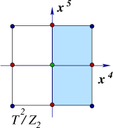
Figure 2: Fixed points of the $Z_{2}$ orbifolding of the torus, here represented by the whole squared (of size $r$) in the $x^{4}$-$x^{5}$ plane. The shadowed region corresponds to the actual fundamental space.

It is certainly impressive that the extra symmetries of the space are just enough as to provide us with an understanding of proton stability. However, the argument has a weakness. It relies on a symmetry which is usually broken by compactification. It is then important to know up to what extent the argument holds on compact space. It actually does, provided the rotational symmetry $U(1)_{45}$ is not completely broken. Consider for instance the orbifold $T^{2}/Z_{2}$, where $T^{2}$ is the torus and $Z_{2}$ the identification $\vec{y}\rightarrow-\vec{y}$, where $\vec{y}=(x^{4},x^{5})$. As it can be seen from Fig. 2, where we have represented the physical compact space on the covering space ${\cal R}^{2}$, the compactification breaks the $SO(1,5)$ group down to $SO(1,3)\times{\cal{Z}}_{4}$, where ${\cal Z}_{4}$ is the group of discrete rotations in the $x^{4}-x^{5}$ plane around the origin by $\pi/2$, a subgroup of $U(1)_{45}$. Clearly, this rotation maps fixed points into themselves. For fermions ${\cal{Z}}_{4}$ rotations become ${\cal{Z}}_{8}$ rotations. Any operator in the effective theory should be invariant under these transformations generated by the same $\Sigma_{45}$ matrix. Therefore, any fermionic operator should satisfy the selection rule

$$\Delta\Sigma_{45}=0~{}~{}mod~{}8~{}.$$ (97)

Usual dimension 10 operators $LQQQ$ (dimension 6 in 4D), do not fulfill this rule, and thus, they remain forbidden. The dimension 16 operators mentioned above do remain, and so does a suppressed proton decay.

It is worth noticing that because charge conjugation operator, $C$, is such that it commutes with 6D chiral operator, $\Gamma_{7}$, which implies that $(\Psi_{\pm})^{C}=(\Psi^{C})_{\pm}$, and also because $C$ anticommutes with $\Sigma_{45}$, there are not Majorana mass terms for neutrinos in these theories. The neutrino should rather be a Dirac field. In the SM presented above, if $N_{R}$ is the even part of the field, then Dirac mass terms, $\bar{L}HN_{R}$, are indeed possible. Smallness is, however, unnatural. One should relay in very small Yukawa couplings. On the other hand, if one rather choose $N_{R}$ to be and odd field, so that $N_{L}$ is even, and extend the gauge sector to contain $B-L$, a solution may be at hand 6dlr . In such a case $\bar{L}HN_{R}$ does not give neutrino masses ($N_{R}$ has only KK modes), but these may be introduced via non renormalizable operators.

V.3 Split Fermions. Hierarchies without Symmetries

Another interesting mechanism that explain how proton decay could get suppressed at the proper level appeared in sch1 . It relays on the idea that the branes are being formed from an effective mechanism that traps the SM particles in it, resulting in a wall with thickness $L\sim M_{\ast}^{-1}$, where the fermions are stuck at different points. Then, fermion-fermion couplings get suppressed due to the exponentially small overlaps of their wave functions. This provides a framework for understanding both the fermion mass hierarchy and proton stability without imposing extra symmetries, but rather in terms of a higher dimensional geography sch2 . Note that the dimension where the gauge fields propagate does not need to be orthogonal to the millimetric dimensions, but gauge fields may be restricted to live in a smaller part of that extra dimensions. Here we briefly summarize those ideas.

V.3.1 Localizing wave functions on the brane.

Let us start by assuming that translational invariance along the fifth dimension is being broken by a bulk scalar field $\Phi$ which develops a spatially varying expectation value $\langle\Phi\rangle(y)$. We assume that this expectation value have the shape of a domain wall transverse to the extra dimension and is centered at $y=0$. With this background a bulk fermion will have a zero mode that is stuck at the zero of $\langle\Phi(y)\rangle$. To see this let us consider the action

$$S=\int d^{4}x\ {\rm d}y\,\overline{\Psi}\left[i\,\Gamma^{M}\!\partial_{M}+\langle\Phi\rangle(y)\right]\Psi,$$ (98)

in the chiral basis given by Eqs. (35) and (36) . By introducing the expansions

$$\psi_{L}(x,y)=\sum_{n}f_{n}(y)\psi_{nL}(x);\qquad\mbox{ and }\qquad\psi_{R}(x,y)=\sum_{n}g_{n}(y)\psi_{nR}(x);$$ (99)

where $\psi_{n}$ are four dimensional spinors, we get for the $y$-dependent functions $f_{n}$ and $g_{n}$ the equations

$$\left(\partial_{5}+\langle\Phi\rangle\right)f_{n}+m_{n}g_{n}=0;\qquad\mbox{ and }\qquad\left(-\partial_{5}+\langle\Phi\rangle\right)g_{n}+m_{n}f_{n}=0;$$ (100)

where now $m_{n}^{2}=p_{\mu}p^{\mu}$ stands for the 4D mass parameter. Therefore, the zero modes have the profiles sch1

$$f_{0}(y)\sim\exp\left[-\int^{y}_{0}\!ds\langle\Phi\rangle(s)\right]\qquad\mbox{ and }\qquad g_{0}(y)\sim\exp\left[\int^{y}_{0}ds\langle\Phi\rangle(s)\right];$$ (101)

up to normalization factors. Notice that when the extra space is supposed to be finite, both modes are normalizable. For the special choice $\langle\Phi\rangle(y)=2\mu_{0}^{2}y$, we get $f_{0}$ centered at $y=0$ with the gaussian form

$$f_{0}(y)=\frac{\mu_{0}^{1/2}}{(\pi/2)^{1/4}}\ \exp\left[{-\mu_{0}^{2}{y}^{2}}\right].$$ (102)

The other mode has been projected out from our brane by being pushed away to the end of the space. Thus, our theory in the wall is a chiral theory. Notice that a negative coupling among $\Psi$ and $\phi$ will instead project out the left handed part.

The generalization of this technique to the case of several fermions is straightforward. The action (98) is generalized to

$$S=\int\!d^{5}x\,\sum_{i,j}\bar{\Psi}_{i}[i\,\Gamma^{M}\partial_{M}+\lambda\langle\Phi\rangle-m]_{ij}\Psi_{j}\ ,$$ (103)

where general Yukawa couplings $\lambda$ and other possible five dimensional masses $m_{ij}$ have been considered. For simplicity we will assume both terms diagonal. The effect of these new parameters is a shifting of the wave functions, which now are centered around the zeros of $\lambda_{i}\langle\Phi\rangle-m_{i}$. Taking $\lambda_{i}=1$ with the same profile for the vacuum leads to gaussian distributions centered at $y_{i}=m_{i}/2\mu_{0}^{2}$. Thus, at low energies, the above action will describe a set of non interacting four dimensional chiral fermions localized at different positions in the fifth dimension.

Localization of gauge and Higgs bosons needs extra assumptions. The explanation of this phenomena is close related with the actual way the brane was formed. A field-theoretic mechanism for localizing gauge fields was proposed by Dvali and Shifman shifman and was later extended and applied in dvali . There, the idea is to arrange for the gauge group to confine outside the wall; the flux lines of any electric sources turned on inside the wall will then be repelled by the confining regions outside and forced them to propagate only inside the wall. This traps a massless gauge field on the wall. Since the gauge field is prevented to enter the confined region, the thickness $L$ of the wall acts effectively as the size of the extra dimension in which the gauge fields can propagate. In this picture, the gauge couplings will exhibit power law running above the scale $L^{-1}$.

V.3.2 Fermion mass hierarchies and proton decay.

Let us consider the Yukawa coupling among the Higgs field and the leptons: $\kappa HL^{T}E^{c}$; where the massless zero mode $l$ from $L$ is localized at $y=0$ while $e$ from $E^{c}$ is localized at $y=r$. Let us also assume that the Higgs zero mode is delocalized inside the wall. Then the zero modes term of this coupling will generate the effective Yukawa action

$$S_{Yuk}=\int\!d^{4}x\,\kappa\,h(x)l(x)e^{c}(x)\ \int\!dy\ \phi_{l}(y)\ \phi_{e^{c}}(y)\ ,$$ (104)

where $\phi_{l}$ and $\phi_{e^{c}}$ represent the gaussian profile of the fermionic modes. Last integral gives the overlap of the wave functions, which is exponentially suppressed sch1 as

$$\int\!dy\ \phi_{l}(y)\ \phi_{e^{c}}(y)\ =e^{-\mu_{0}^{2}r^{2}/2}.$$ (105)

This is a generic feature of this models. The effective coupling of any two fermion fields is exponentially suppressed in terms of their separation in the extra space. Thus, the explanation for the mass hierarchies becomes a problem of the cartography on the extra dimension. A more detailed analysis was presented in sch2 .

Let us now show how a fast proton decay is evaded in these models. Assume, for instance, that all quark fields are localized at $y=0$ whereas the leptons are at $y=r$. Then, let us consider the following baryon and lepton number violating operator

$$S\sim\int d^{5}x\,\frac{(Q^{T}C_{5}L)^{\dagger}(U^{cT}C_{5}D^{c})}{M^{3}}.$$ (106)

In the four dimensional effective theory, once we have introduced the zero mode wave functions, we get the suppressed action sch1

$$S\sim\int d^{4}x\,\,\lambda\times\frac{(ql)^{\dagger}(u^{c}d^{c})}{M^{2}}$$ (107)

where $\lambda\sim\int dy\,\left[e^{-\mu_{0}^{2}y^{2}}\right]^{3}e^{-\mu_{0}^{2}(y-r)^{2}}\sim e^{-3/4\mu_{0}^{2}r^{2}}$. Then, for a separation of $\mu_{0}r=10$ we obtain $\lambda\sim 10^{-33}$ which renders these operators completely safe even for $M_{\ast}\sim 1$ TeV. Therefore, we may imagine a picture where quarks and leptons are localized near opposite ends of the wall so that $r\sim L$. This mechanism, however, does not work for suppressing the another dangerous operator $(LH)^{2}/M$ responsible of a large neutrino mass.

VI Warped Extra Dimensions

So far we have been working in the simplest picture where the energy density on the brane does not affect the space time curvature, but rather it has been taken as a perturbation on the flat extra space. However, for large brane densities this may not be the case. The first approximation to the problem can be done by considering a five dimensional model where branes are located at the two ends of a closed fifth dimension. Clearly, with a single extra dimension, the gravity flux produced by a single brane at $y=0$ can not softly close into itself at the other end the space, making the model unstable, just as a charged particle living in a closed one-dimensional world does not define a stable configuration. Stability can only be insured by the introduction of a second charge (brane). Furthermore, to balance branes energy and still get flat (stable) brane metrics, one has to compensate the effect on the space by the introduction of a negative cosmological constant on the bulk. Hence, the fifth dimension would be a slice of an Anti de-Siter space with flat branes at its edges. Thus, one can keep the branes flat paying the price of curving the extra dimension. Such curved extra dimensions are usually referred as warped extra dimensions. Historically, the possibility was first mentioned by Rubakov and Shaposhnikov in Ref. rubakov , who suggested that the cosmological constant problem could be understood under this light: the matter fields vacuum energy on the brane could be canceled by the bulk vacuum, leaving a zero (or almost zero) cosmological constant for the brane observer. No specific model was given there, though. It was actually Gogberashvili merab who provided the first exact solution for a warped metric, nevertheless, this models are best known after Randall and Sundrum (RS) who linked the solution to the the hierarchy problem rs1 . Later developments suggested that the warped metrics could even provide an alternative to compactification for the extra dimensions rs2 ; nimars . In what follows we shall discuss a concrete example as presented by Randall and Sundrum.

VI.1 Randall-Sundrum Background and the Hierarchy Problem

VI.1.1 Randall-Sundrum background.

Lets consider the following setup. A five dimensional space with an orbifolded fifth dimension of radius $r$ and coordinate $y$ which takes values in the interval $[0,\pi r]$. Consider two branes at the fixed (end) points $y=0,\pi r$; with tensions $\tau$ and $-\tau$ respectively. For reasons that should become clear later on, the brane at $y=0$ ($y=\pi r$) is usually called the hidden (visible) or Planck (SM) brane. We will also assign to the bulk a negative cosmological constant $-\Lambda$. Contrary to our previous philosophy, here we shall assume that all parameters are of the order of the Planck scale. Next, we ask for the solution that gives a flat induced metric on the branes such that 4D Lorentz invariance is respected. To get a consistent answer, one has to require that at every point along the fifth dimension the induced metric should be the ordinary flat 4D Minkowski metric. Therefore, the components of the 5D metric only depend on the fifth coordinate. Hence, one gets the ansatz

$$ds^{2}=g_{AB}dx^{A}dx^{B}=\omega^{2}(y)\eta_{\mu\nu}dx^{\mu}dx^{\nu}-dy^{2}~{},$$ (108)

where we parameterize $\omega(y)=e^{-\beta(y)}$. The metric, of course, can always be written in different coordinate systems. Particularly, notice that one can easily go to the conformally flat metric, where there is an overall factor in front of all coordinates, $ds^{2}=\omega^{2}(z)[\eta_{\mu\nu}dx^{\mu}dx^{\nu}-dz^{2}]$, where the new coordinate $z$ is a function of the old coordinate $y$ only.

Classical action contains $S=S_{grav}+S_{h}+S_{v}$; where

$$S_{grav}=\int\!d^{4}x\,dy\sqrt{g_{(5)}}\left(\frac{1}{2k_{\ast}^{2}}R_{5}+\Lambda\right)~{},$$ (109)

gives the bulk contribution, whereas the visible and hidden brane parts are given by

$$S_{v,h}=\pm~{}\tau~{}\int\!d^{4}x\sqrt{-g_{v,h}}~{},$$ (110)

where $g_{v,h}$ stands for the induced metric at the visible and hidden branes, respectively. Here $\kappa_{\ast}^{2}=8\pi G_{\ast}=M_{\ast}^{-3}$.

Five dimensional Einstein equations for the given action become

$$G_{MN}=-k_{\ast}^{2}\Lambda\,g_{MN}+k_{\ast}^{2}\tau\,\sqrt{\frac{-g_{h}}{g_{(5)}}}\delta_{M}^{\mu}\delta_{N}^{\nu}g_{\mu\nu}\delta(y)-k_{\ast}^{2}\tau\,\sqrt{\frac{-g_{v}}{g_{(5)}}}\delta_{M}^{\mu}\delta_{N}^{\nu}g_{\mu\nu}\delta(y-\pi r)$$

where the Einstein tensor $G_{MN}=R_{MN}-\frac{1}{2}g_{MN}R_{(5)}$ as usual. They are easily reduced into two simple independent equations. First, we can expand the $G_{MN}$ tensor components using the metric ansatz (108) to show that

$$G_{\mu\nu}=-3\,g_{\mu\nu}\left(-\beta^{\prime\prime}+2(\beta^{\prime})^{2}\right)~{};\quad G_{\mu 5}=0~{};\quad\mbox{ and }\quad G_{55}=-6\,g_{55}(\beta^{\prime})^{2}~{}.$$ (111)

Next, using the RHS of Eq. (VI.1.1), one gets that $6(\beta^{\prime})^{2}=k_{\ast}^{2}\Lambda$, and

$$3\beta^{\prime\prime}=k_{\ast}^{2}\tau\,\left[\delta(y)-\delta(y-\pi r)\right].$$ (112)

Last equation, clearly, defines the boundary conditions for the function $\beta^{\prime}(y)$ at the two branes (Israel conditions). Clearly, the solution is $\beta(y)=\mu|y|$, where

$$\mu^{2}=\frac{k_{\ast}^{2}\Lambda}{6}=\frac{\Lambda}{6M_{\ast}^{3}}~{},$$ (113)

with the subsidiary fine tuning condition

$$\Lambda=\frac{\tau^{2}}{6M_{\ast}^{3}}~{},$$ (114)

obtained from the boundary conditions, that is equivalent to the exact cancellation of the effective four dimensional cosmological constant. The background metric is therefore

$$ds^{2}=e^{-2\mu|y|}\eta_{\mu\nu}dx^{\mu}dx^{\nu}-dy^{2}~{}.$$ (115)

The effective Planck scale in the theory is then given by

$$M_{P}^{2}=\frac{M_{\ast}^{3}}{\mu}\left(1-e^{-2\mu r\pi}\right).$$ (116)

Notice that for large $r$, the exponential piece becomes negligible, and above expression has the familiar form given in Eq. (10) for one extra dimension of (effective) size $1/\mu$.

VI.1.2 Visible versus Hidden Scales Hierarchy.

The RS metric has a peculiar feature. Consider a given distance, $ds_{0}^{2}$, defined by fixed intervals $dx_{\mu}dx^{\mu}$ from brane coordinates. If one maps the interval from hidden to visible brane, it would appear here exponentially smaller than what is measured at the hidden brane, i.e., $ds_{0}^{2}|_{v}=\omega^{2}(\pi r)ds_{0}^{2}|_{h}$. This scaling property would have interesting consequences when introducing fields to live on any of the branes. Particularly, let us discuss what happens for a theory defined on the visible brane.

The effect of RS background on visible brane field parameters is non trivial. Consider for instance the scalar field action for the visible brane at the end of the space given by

$$S_{H}=\int\!d^{4}x\,\omega^{4}(\pi r)\left[\omega^{-2}(\pi r)\partial^{\mu}H\partial_{\mu}H-\lambda\left(H^{2}-\hat{v}_{0}^{2}\right)^{2}\right].$$

As a rule, we choose all dimensionful parameters on the theory to be naturally given in terms of $M_{\ast}$, and this to be close to $M_{P}$. So we take $\hat{v}_{0}\sim M_{\ast}$. After introducing the normalization $H\rightarrow\omega^{-1}(\pi r)H=e^{\mu r\pi}H$ to recover the canonical kinetic term, the above action becomes

$$S_{H}=\int\!d^{4}x\left[\partial^{\mu}H\partial_{\mu}H-\lambda\left(H^{2}-v^{2}\right)^{2}\right],$$ (117)

where the actual vacuum $v=e^{-\mu r\pi}\hat{v}_{0}$. Therefore, by choosing $\mu r\sim 12$, the physical mass of the scalar field, and its vacuum, would naturally appear at the TeV scale rather than at the Planck scale, without the need of any large hierarchy on the radius rs1 . Notice that, on the contrary, any field located on the other brane will get a mass of the order of $M_{\ast}$. Moreover, it also implies that no particles exist in the visible brane with masses larger than TeV. This observation has been consider a nice possible way of solving the scales hierarchy problem. For this reason, the original model proposed that our observable Universe resides on the brane located at the end of the space, the visible brane. So the other brane really becomes hidden. This two brane model is sometimes called RSI model.

VI.2 KK Decomposition on RS

As a further note, notice that since there is everywhere 4D Poincaré invariance, every bulk field on the RS background can be expanded into four dimensional plane waves $\phi(x,y)\propto e^{ip_{\mu}x^{\mu}}\varphi(y)$. This would be the basis for the Kaluza Klein decomposition, that we shall now discuss. Note also that the physical four momentum of the particle at any position of the brane goes as $p_{phys}^{\mu}(y)=\omega^{-1}(y)p^{\mu}$. Therefore, modes which are soft on the hidden brane, become harder at any other point of the bulk.

Lets consider again a bulk scalar field, now on the RS background metric. The action is then

$$S[\phi]=\frac{1}{2}\int\!d^{4}x\,dy\sqrt{g_{(5)}}\left(g^{MN}\partial_{M}\phi\partial_{N}\phi-m^{2}\phi^{2}\right)~{}.$$ (118)

By introducing the factorization $\phi(x,y)=e^{ip_{\mu}x^{\mu}}\varphi(y)$ into the equation of motion, one gets that the KK modes satisfy

$$\left[-\partial_{y}^{2}+4\mu~{}{\rm sgn}(y)\partial_{y}+m^{2}+\omega^{-2}(y)\,p^{2}\right]\varphi(y)=0~{},$$ (119)

where $p^{2}=p^{\mu}p_{\mu}$ can also be interpreted as the effective four dimensional invariant mass, $m_{n}^{2}$. It is possible, through a functional re-parameterization and a change of variable, to show that the solution for $\varphi$ can be written in terms of Bessel functions of index $\nu=\sqrt{4+m^{2}/\mu^{2}}$ gw0 ; Rubakov2 , as follows

$$\varphi_{n}(y)=\frac{1}{N_{n}\omega^{2}(y)}\,\left[J_{\nu}\left(\frac{m_{n}}{\mu\omega(y)}\right)+b_{n\nu}Y_{\nu}\left(\frac{m_{n}}{\mu\omega(y)}\right)\right]\,,$$ (120)

where $N_{n}$ is a normalization factor, $n$ labels the KK index, and the constant coefficient $b_{n\nu}$ has to be fixed by the continuity conditions at one of the boundaries. The other boundary condition would serve to quantize the spectrum. For more details the reader can see Ref. gw0 . Here we will just make some few comments about. First, for $\omega(\pi r)\ll 1$, the discretization condition that one gets for $x_{n\mu}=m_{n}/\mu\omega(y)$ looks as

$$2J_{\nu}(x_{n\mu})+x_{n\nu}J^{\prime}_{\nu}(x_{n\mu})=0~{}.$$ (121)

Therefore, the lowest mode satisfies $x_{1\mu}\sim{\cal O}(1)$, which means that $m_{1}\simeq\mu e^{-\mu r\pi}$. For the same range of parameters we considered before to solve the hierarchy problem, one gets that lightest KK mode would have a mass of order TeV or so. Next, for the special case of a originally massless field ($m=0$), one has $\nu=2$, and thus the first solution to Eq. (121) is just $x_{12}=0$, which indicates the existence of a massless mode in the spectrum. The next zero of the equation would be of order one again, thus the KK tower would start at $\mu e^{-\mu r\pi}$. The spacing among two consecutive KK levels would also be of about same order. There is no need to stress that this would actually be the case of the graviton spectrum. This makes the whole spectrum completely distinct from the former ADD model. With such heavy graviton modes one would not expect to have visible deviations on the short distance gravity experiments, nor constrains from BBN, star cooling or astrophysics in general. Even colliders may not be able to test direct production or exchange of such heavy gravitons.

VI.3 Radius Stabilization

The way RSI model solves the hierarchy problem between $m_{EW}$ and $M_{P}$ depends on the interbrane spacing $\pi r$. Stabilizing the bulk becomes in this case an important issue if one is willing to keep this solution. The dynamics of the extra dimension would give rise to a running away radion field, similarly as it does for the ADD case. A simple exploration of the metric (115), by naively setting a slowly time dependent bulk radius $r(t)$, shows that

$$ds^{2}\rightarrow e^{-2\mu r(t)|\phi|}\eta_{\mu\nu}dx^{\mu}dx^{\nu}-r^{2}(t)d\theta^{2}~{};$$ (122)

with $\theta$ the angular coordinate on the half circle $[0,\pi]$. This suggest that if the interbrane distance changes the visible brane expands (or contracts) exponentially. The radion field associated to the fluctuations of the radius, $b(t)=r(t)-r$, is again massless and thus it violates the equivalence principle. Moreover, without a stabilization mechanism for the radius, our brane could expand forever. Some early discussions on this and other issues can be found in Refs. gw ; rsradion ; rrs1 .

A simple and elegant solution for stabilization in RSI was proposed by Goldberger and Wise gw . The central idea is as follows: if there is a vacuum energy on the bulk, whose configuration breaks translational invariance along fifth dimension, say $\langle E\rangle(y)$, then, the effective four dimensional theory would contain a radius dependent potential energy

$$V(r)=\int\!dy\,\omega^{4}(y)\,\langle E\rangle(y)~{}.$$

Clearly, if such a potential has a non trivial minimum, stabilization would be insured. The radion would feel a force that tends to keep it at the minimum. The vacuum energy $\langle E\rangle(y)$ may come from many sources. The simplest possibility one could think up on is a vacuum induced by a bulk scalar field, with non trivial boundary conditions,

$$\langle\phi\rangle(0)=v_{h}\qquad\mbox{ and }\qquad\langle\phi\rangle(\pi r)=v_{v}~{}.$$ (123)

The boundary conditions would amount for a non trivial profile of $\langle\phi\rangle(y)$ along the bulk. Such boundary conditions may arise, for instance, if $\phi$ has localized interaction terms on the branes, as $\lambda_{h,v}(\phi^{2}-v_{h,v}^{2})^{2}$, which by themselves develop non zero vacuum expectation values for $\phi$ located on the branes. The vacuum is then the $x$ independent solution to the equation of motion (119), which can be written as $\langle\phi\rangle(y)=\omega^{-1}(y)\left[A\omega^{-\nu}(y)+B\omega^{\nu}(y)\right]$, where $A$ and $B$ are constants to be fixed by the boundary conditions. One then obtains the effective 4D vacuum energy

$$V_{\phi}(r)=\mu(\nu+2)A^{2}\left(\omega^{-2\nu}(\pi r)-1\right)+\mu(\nu-2)B^{2}\left(1-\omega^{2\nu}(\pi r)\right)$$ (124)

After a lengthly calculation, in the limit where $m\ll\mu$ one finds that above potential has a non trivial minimum for

$$\mu r=\left(\frac{4}{\pi}\right)\frac{\mu^{2}}{m^{2}}\ln\left[\frac{v_{h}}{v_{v}}\right]~{}.$$ (125)

Hence, for $\ln(v_{h}/v_{v})$ of order one, the stable value for the radius goes proportional to the curvature parameter, $\mu$, and inversely to the squared mass of the scalar field. Thus, one only needs that $m^{2}/\mu^{2}\sim 10$ to get $\mu r\sim 10$, as needed for the RSI model.

One can get a bit suspicious about whether the vacuum energy $\langle\phi\rangle(y)$ may disturb the background metric. It actually does, although the correction is negligible as the calculations for the Einstein-scalar field coupled equations may show gw ; rrs1 .

VI.4 RSII: A Non Compact Extra Dimension

The background metric solution (115) does not actually need the presence of the negative tension brane to hold as an exact solution to Einstein equations. Indeed the warp factor $\omega(y)=e^{-\mu|y|}$ has been determined only by the Israel conditions at the $y=0$ boundary. That is, by using $\omega^{\prime\prime}=\mu^{2}\omega-\mu\omega\delta(y)$ in Einstein equations, which implies equations (113) and (114). It is then tempting to ‘move’ the negative tension brane to infinity, which renders a non compact fifth dimension. The picture becomes esthetically more appealing, it has no need for compactification. Nevertheless, one has to ask now the question of whether such a possibility is at all consistent with observations. It is clear that the Newton’s constant is now simply

$$G_{N}=\mu G_{\ast}~{}$$ (126)

–just take the limit $r\rightarrow\infty$ in Eq. (116)–, this reflects the fact that although the extra dimension is infinite, gravity remains four dimensional at large distances (for $\mu r\gg 1$). This is, in other words, only a consequence of the flatness of the brane. We shall expand our discussion on this point in following sections. Obviously, with this setup, usually called the RSII model rs2 , we are giving up the possibility of explaining the hierarchy between Planck and electroweak scales. The interest on this model remains, however, due to potentially interesting physics at low energy, and also due to its connection to the AdS/CFT correspondence ads/cft .

Although the fifth dimension is infinite, the point $y=\infty$ is in fact a particle horizon. Indeed, the first indication comes from the metric, since $\omega(y\rightarrow\infty)=0$. The confirmation would come from considering a particle moving away from the brane on the geodesics $y_{g}(t)=\frac{1}{2\mu}\ln(1+\mu^{2}t^{2})$ ruba . The particle accelerates towards infinity, and its velocity tends to speed of light. The proper time interval is then

$$d\tau^{2}=\omega^{2}(y_{g}(t))dt^{2}-\left(\frac{dy_{g}}{dt}\right)^{2}dt^{2}~{}.$$ (127)

Thus, the particle reaches infinity at infinite time $t$, but in a finite proper time $\tau=\pi/2\mu$.

VI.5 Graviton Localization

In order to understand why gravity on the brane remains four dimensional at large distances, even though the fifth dimension is non compact, one has to consider again the KK decomposition for the graviton modes, with particular interest on the shape for the zero mode wave function rs2 . Consider first the generic form of the perturbed background metric

$$ds^{2}=\omega^{2}(y)g_{\mu\nu}dx^{\mu}dx^{\nu}+A_{\mu}dx^{\mu}dy-b^{2}dy^{2}~{}.$$

Due to the orbifold projection $y\rightarrow-y$, the vector component $A_{\mu}$ has to be odd, and thus it does not contain a zero mode. Therefore at the zero mode level only the true four dimensional graviton and the scalar (radion) should survive. Let us concentrate on the 4D graviton perturbations only. Introducing the small field expansion as $g_{\mu\nu}=\eta_{\mu\nu}+\omega^{-2}h_{\mu\nu}$, and using the gauge fixing conditions $\partial_{\mu}h^{\mu}_{\nu}=0=h^{\mu}_{\mu}$, one obtains the wave equation

$$\left[\partial_{y}^{2}-4\mu^{2}-\frac{m^{2}}{\omega^{2}(y)}-4\mu\delta(y)\right]h=0~{};$$ (128)

where the Lorentz indices should be understood. In the above equation the mass $m^{2}$ stands for the effective four dimensional mass $p^{\mu}p_{\mu}=m^{2}$. It should be noticed that the mass spectrum would now be continuous and starts at $m=0$. In this situation the KK are normalized to a delta function, $\int\!dy~{}\omega^{-2}(y)\,h_{m}(y)\,h_{m^{\prime}}=\delta(m-m^{\prime})$.

Introducing the functional re-parameterization $z=sgn(y)\,\left(\omega^{-1}(y)-1\right)/\mu$ and $\Psi(z)=\omega^{-1/2}(y)~{}h(y)$; one can write the equation of motion for the KK modes as the Scrhödinger equation rs2

$$\left[-\frac{1}{2}\partial_{z}^{2}+V(z)\right]\Psi(z)=m^{2}\Psi(z)$$ (129)

with a ‘volcano potential’

$$V(z)=\frac{15\mu^{2}}{8(\mu|z|+1)^{2}}-\frac{3\mu}{2}\delta(z)~{},$$ (130)

which peaks as $|z|\rightarrow 0$ but has a negative singularity right at the origin. It is well known from the quantum mechanics analog that such delta potential has a bound state, whose wave function is peaked at $z=0$, which also means at $y=0$. In other words, there is a mode that appears as to be localized at the brane. Such a state is identified as our four dimensional graviton. Its localization is the physical reason why gravity still behaves as four dimensional at the brane.

Indeed, the wave function for the localized state goes as

$$\Psi_{o}(z)=\frac{1}{\mu(|z|+1/\mu)^{3/2}}$$ (131)

whereas KK mode wave functions in the continuum are written in terms of Bessel functions, in close analogy to Eq. (120), as

$$\Psi_{m}\sim s(z)\left[Y_{2}\left(m|z|+\frac{1}{\mu}\right)+\frac{4\mu^{2}}{\pi m^{2}}J_{2}\left(m|z|+\frac{1}{\mu}\right)\right]$$

where $s(z)=(|z|+1/\mu)^{1/2}$. By properly normalizing these wave functions using the asymptotic for of Bessel functions, it is possible to show that for $m<\mu$ the wave function at brane has the value

$$h_{m}(0)\approx\sqrt{\frac{m}{\mu}}~{}.$$ (132)

The coupling of gravitons to the brane is therefore weak for the lightest KK graviton states. The volcano potential acts as a barrier for those modes. The production of gravitons at low energies would then be negligible.

The immediate application of our last calculations is on the estimation of the effective gravitational interaction law at the brane. The reader should remember that the effective interaction of brane matter to gravitons goes as $h_{\mu\nu}(0)T^{\mu\nu}$. So, it does involve the evaluation of the graviton wave function at the brane position. Graviton exchange between two test particles on the brane separated by a distance $r$ then gives the effective potential rs2grav

$$U_{RSII}(r)\approx U_{N}(r)\left[1+\int_{0}^{\infty}\!\frac{dm}{\mu}\,\frac{m}{\mu}e^{-mr}\right]=U_{N}(r)\left[1+\frac{1}{\mu^{2}r^{2}}\right]~{}.$$ (133)

Notice that the correction looks exactly as in the two extra dimensional ADD case, with $1/\mu$ as the effective size of the extra dimensions. Thus, to the brane the bulk should appear as compact, at least from the gravitational point of view. The conclusion is striking. There could be non compact extra dimensions and yet scape to our observations!.

VI.6 Beyond RSII: More Infinite Extra Dimensions

The RSII model, which provides a serious alternative to compactification, can immediately be extended to have a larger number of dimensions. First, notice that the metric (115) came out of the peculiar properties of co-dimension one objects in gravity. Thus, it is obvious that the straightforward generalization should also contain some co-dimension one branes in the configuration. Our brane, however should have a larger co-dimension. Lets consider a system of $n$ mutually intersecting $(2+n)$ branes in a $(4+n)$ dimensional AdS space, of cosmological constant $-\Lambda$. All branes should have a positive tension $\tau$. Clearly, the branes intersection is a 4 dimensional brane, where we assume our Universe lives. Intuitively, each of the $(2+n)$ branes would try to localize the graviton to itself, just as the RSII brane does. As a consequence, the zero mode graviton would be localized at the intersection of all branes. This naive observation can indeed be confirmed by solving the Einstein equations for the action nimars

$$S=\int\!d^{4}x\,d^{n}y\,\sqrt{|g_{(4+n)}|}\left(\frac{1}{2k_{\ast}}R_{(4+n)}+\Lambda\right)-\sum_{\mbox{all branes}}\tau\,\int\!d^{4}x\,d^{n-1}y\,\sqrt{|g_{(3+n)}|}$$ (134)

If the branes are all orthogonal to each other, it is straightforward to see that the space consist of $2^{n}$ equivalent slices of AdS space, glued together along the flat branes. The metric, therefore, would be conformally flat. Thus, one can write it down using appropriate bulk coordinates as

$$ds_{(4+n)}^{2}=\Omega(z)\left(\eta_{\mu\nu}dx^{\mu}dx^{\nu}-\delta_{kl}\,dz^{k}dz^{l}\right)$$ (135)

with the warp factor $\Omega(z)=(\mu\sum_{j}|z^{i}|+1)^{-1}$; where the $\mu$ curvature parameter is now

$$\mu^{2}=\frac{2k_{\ast}^{2}\Lambda}{n(n+2)(n+3)};$$ (136)

which is a generalization of the relation given in Eq. (113). Similarly, the fine tuning condition (114), now looks as

$$\Lambda=\frac{n(n+3)}{8(n+2)}\tau^{2}k_{\ast}^{2}~{}.$$ (137)

Effective Planck scale is now calculated to be

$$M_{P}^{2}=M_{\ast}^{(n+2)}\int\!d^{n}z\Omega^{(2+n)}=\frac{2^{n}n^{n/2}}{(n+1)!}M_{\ast}^{(n+2)}L^{n}~{},$$ (138)

for $L=1/\sqrt{n}\mu$. Notice this expression resembles the ADD relationship given in Eq. (10), with the effective size of the extra dimensions proportional to $L$.

Graviton localization can be now seen by perturbing the metric with $\eta_{\mu\nu}\rightarrow\eta_{\mu\nu}+h_{\mu\nu}$ in Eq. (135), and writing down the equation of motion for $h_{\mu\nu}$ in the gauge ${h^{\mu}}_{\mu}=0=\partial_{\mu}h^{\mu\nu}$, and in conformal coordinates, to get for $\Psi=\Omega^{(n+2)/2}h$ the linearized equation

$$\left[-\frac{1}{2}m^{2}+\left(-\frac{1}{2}\nabla_{z}^{2}+V(z)\right)\right]\hat{\Psi}=0~{},$$ (139)

which is again nothing but a Schrödinger equation with the effective potential

$$V(z)=\frac{n(n+2)(n+4)\mu^{2}}{8}\Omega-\frac{(n+2)\mu}{2}\Omega\sum_{j}\delta(z^{j})$$ (140)

Indeed, the spectrum has a massless bound state localized around the intersection of all delta function potentials ($z=0$), which goes as $\Psi_{bound}\sim\Omega^{(n+2)/2}(z)$. Since the potential falls off to zero at large $z$, there would also be a continuum of modes. Since the height of the potential near the origin goes as $\mu^{2}$, all modes with small masses, $m<\mu$ will have suppressed wave functions, whereas those with large masses will be un-suppressed at the origin. Therefore, the contribution of the lightest modes to gravitational potential for two test particles at the brane would again come suppressed as in the RSII case. The correction to Newton’s law goes as nimars

$$\Delta U(r)\sim U_{N}(r)\left(\frac{L}{r}\right)^{n}~{},$$ (141)

which again behaves as in the ADD case, mimicking the case of compact dimensions, thought there are not so.

VII Concluding remarks

Along the present notes we have introduced the reader to some aspects of models with extra dimensions where our Universe is constrained to live on a four dimensional hypersurface. The study of models with extra dimensions has become a fruitful industry that has involved several areas of theoretical physics in matter of few years. It is fair to say, however, that many of the current leading directions of research obey more to speculative ideas that to well established facts. Nevertheless, the studies on the brane world are guided by the principle of physical and mathematical consistency, and inspired on the possibility of connecting, at some point, the models with a more fundamental theory, perhaps String theory from where the idea of extra dimensions and branes had been borrowed. Further motivation also comes from the possibility of experimentally testing these ideas within the near future, something that was just unthinkable in many old models where the fundamental gravity scale was the Planck scale.

It is hard to address the too many interesting topics of the area in detail, as we would have liked, without facing trouble with the limiting space of this short notes. In exchange, we have concentrated the discussion to the construction of the main frameworks (ADD, and RS models), paying special attention to dimensional reduction and some of the interesting phenomenology of quantum gravity in colliders as well as in BBN and astrophysics. We have also discussed at some extend the calculation of the effective gravity interactions on the brane. Some applications and uses in model building for the extra dimensions have also been addressed, including the promotion of SM fields to the bulk and the consequent power law running of couplings as well as some ideas on symmetry breaking with extra dimensions. We have also commented some ideas to get a small neutrino mass and a very stable proton despite the possibility of having a low fundamental scale. The basis of RS models have also been discussed in some detail.

I hope these notes could serve the propose of been a brief introduction to this area of research. The list of topics we have been unable to cover is extensive, it includes many issues on cosmology of models with flat and warped extra dimensions cosmo1 ; cosmo2 ; the discussions on the cosmological constant problem cc , higher dimensional warped spaces hdw ; dark matter from KK modes dmkk , many ideas on Black Holes in both ADD and RS models bh1 ; rsbh , deconstruction of extra dimensions deconstruction , and the list go on. I hope the interested readers could consult other reviews reviews and search for further references.