SLAC-PUB-11036 March 2005

Collider Production of TeV Scale Black Holes and Higher-Curvature Gravity

Thomas G. Rizzo^a

Stanford Linear Accelerator Center, 2575 Sand Hill Rd., Menlo Park, CA, 94025

We examine how the production of TeV scale black holes at colliders is influenced by the presence of Lovelock higher-curvature terms in the action of models with large extra dimensions. Such terms are expected to arise on rather general grounds, e.g., from string theory and are often used in the literature to model modifications to the Einstein-Hilbert action arising from quantum and/or stringy corrections. While adding the invariant which is quadratic in the curvature leads to quantitative modifications in black hole properties, cubic and higher invariants are found to produce significant qualitative changes, e.g., classically stable black holes. We use these higher-order curvature terms to construct a toy model of the black hole production cross section threshold. For reasonable parameter values we demonstrate that detailed measurements of the properties of black holes at future colliders will be highly sensitive to the presence of the Lovelock higher-order curvature terms.

1 Introduction

The introduction of large extra dimensions by Arkani-Hamed, Dimopoulos and Dvali[1] offers us the possibility that the true fundamental scale of gravity, $M_{*}$, may not be too far above the weak scale, $\sim$ TeV. In this scenario, gravity is allowed to propagate in all $D=4+n$ dimensions while the Standard Model(SM) fields are confined to live on a three-dimensional ’brane’ which we assume to be flat. One then finds $M_{*}$ is related to the usual 4-d (reduced) Planck scale, $\overline{M}_{Pl}$, via the now famous expression

$$\overline{M}_{Pl}^{2}=V_{n}M_{*}^{n+2}\,,$$ (1)

where $V_{n}$ is the volume of the compactified extra dimensions. These compactified dimensions are usually assumed to be flat, i.e., they form an $n$-dimensional torus so that, if all compactification radii, $R_{c}$, were the same, $V_{n}=(2\pi R_{c})^{n}$. This simple ADD picture has three basic predictions that have gotten significant attention in the literature[2] over the past few years: ($i$) the emission of graviton Kaluza-Klein states during the collision of SM particles leading to final states with apparent missing energy[3, 4, 5]; ($ii$) the exchange of graviton Kaluza-Klein excitations between SM fields leading to new dimension-8 contact interaction-like operators with distinctive spin-2 properties[3, 4, 6]; ($iii$) the production of black holes(BH) at colliders and in cosmic rays with geometric subprocess cross sections once energies greater than $\sim M_{*}$ are exceeded[7, 8, 9, 10]. While ($i$) and ($ii$) result from an expansion of the gravitational action, i.e., the $D-$dimensional Einstein-Hilbert(EH) action, to leading order in the gravitational field and are in some sense perturbative, ($iii$) on the other-hand relies upon the full non-perturbative content of the EH action. Here one is really testing $D-$dimensional General Relativity and not just the ADD picture. Within the ADD scenario, collider measurements of ($i$) and ($ii$) type processes will tell us the values of $n$ and $M_{*}$[2].

If anything like the ADD scenario is realized in Nature it will have to be part of a much larger framework, i.e., ADD is at best an effective theory that operates at energies below the scale $M_{*}$. It is reasonable to expect that at least some aspects of this more complete theory may leak down into the collider tests listed above and may lead to significant quantitative and/or qualitative modifications that can be probed experimentally. Here we examine one such extension of the basic model: the existence of higher curvature terms which augment the EH action. Such terms are expected to be present at some level on rather general grounds from string theory[11, 12] or other possible high-scale completions of General Relativity. These terms can also be thought of as being generated by quantum corrections to the ordinary EH action. Given arbitrary powers and derivatives of the curvature tensor there are a huge number of possible higher-order invariants from which to choose. In order to decide what to add to the EH action we need some form of guidance in making possible selections.

Fortunately, a certain special class of such invariants with very interesting properties was first generally described long ago by Lovelock[13] and, hence, are termed Lovelock invariants. These are constructed out of powers of the curvature tensor with no additional derivatives. They are also sometimes referred to in the literature as generalized Euler densities since their volume integrals are related to the Euler characteristics. These Lovelock invariants themselves come in fixed order, $m$, which we denote here as ${\cal L}_{m}$, that describes the number of powers of the curvature tensor, contracted in various ways, out of which they are constructed. Apart from normalization factors we can express the ${\cal L}_{m}$ as

$${\cal L}_{m}\sim\delta^{A_{1}B_{1}...A_{m}B_{m}}_{C_{1}D_{1}...C_{m}D_{m}}~{}R_{A_{1}B_{1}}~{}^{C_{1}D_{1}}.....R_{A_{m}B_{m}}~{}^{C_{m}D_{m}}\,,$$ (2)

where $\delta^{A_{1}B_{1}...A_{m}B_{m}}_{C_{1}D_{1}...C_{m}D_{m}}$ is the totally antisymmetric product of Kronecker deltas and $R_{AB}~{}^{CD}$ is the $D$-dimensional curvature tensor. Fortunately, as can be seen by this definition, the number of such invariants that can exist in any given dimension is highly constrained. For a space with an even number of dimensions, $D=2m$, the Lovelock invariant is a topological one and leads to a total derivative, i.e., a surface term, in the action. All of the higher order invariants, $D\leq 2m-1$, can then be shown to vanish identically by various curvature tensor index symmetry properties. On the otherhand, for the cases with $D\geq 2m+1$, the ${\cal L}_{m}$ are true dynamical objects that once added the action can significantly alter the field equations normally associated with the EH term. However it can be shown that the addition of any or all of the ${\cal L}_{m}$ to the EH action still results in a theory with only second order equations of motion as is the case for ordinary Einstein gravity. Furthermore, variation of the new action leads to modifications of Einstein’s equations by the addition of new terms which are second-rank symmetric tensors with vanishing covariant derivatives and which depend only on the metric and its first and second derivatives, i.e., they have the same general properties as the Einstein tensor itself but are higher order in the curvature. These properties are quite special. Generally, the addition to the action of arbitrary invariants formed from ever higher powers of the curvature tensor will lead to equations of motion of ever higher order, i.e., ever more co-ordinate derivatives of the metric tensor and graviton field, e.g., terms with quartic derivatives. Such theories will have very serious problems with both the presence of ghosts as well as with unitarity[11]. The Lovelock invariants are constructed in such a way as to be free of these problems making them quite exceptional. Interestingly the Lovelock invariants are found to be just the forms taken by the higher order curvature terms generated in perturbative critical string theory[11, 12]. This is perhaps what we might have expected if string theories are to avoid these troublesome ghost and unitarity issues.

In the case of the ADD model, we are generally considering the possibility that the number of extra dimensions lies in the range $2\leq n\leq 6$. We now imagine extending the $D$-dimensional EH action of ADD to include all of the allowable Lovelock invariants for a given value of $n$ with arbitrary coefficients. What do these additional terms do? Firstly, as we will see below based on simple dimensional analysis, these new invariants are suppressed in comparison to the usual EH action by powers of $M_{*}$ and so are only important as TeV-scale energies are approached. Secondly, a short amount of algebra demonstrates that their impact on the ADD model itself is rather subtle since the compactified space is assumed to be flat and the SM fields are restricted to a 3-brane. In particular the leading-order expression for the interaction of the graviton Kaluza-Klein modes, $h_{\mu\nu}^{(n)}$ with the localized SM fields remains as in the EH case:

$$S_{int}=\int d^{4}x~{}d^{n}y~{}{-1\over{M_{*}^{1+n/2}}}\sum_{n}h_{\mu\nu}^{(n)}T^{\mu\nu}\delta(y)\,,$$ (3)

where $T^{\mu\nu}$ is the stress-energy tensor for the SM fields and with $y$ labeling the coordinates of the compactified torus. (Graviton self-interactions, not generally probed in the ADD scenario are modified by the Lovelock terms.) The mass spectrum of the graviton KK states is also unchanged. This means that the signals ($i$) and ($ii$) remain unaltered by these modifications to the ADD action. Note that if the geometry of space was curved, as in the Randall-Sundrum model[14], the couplings of graviton Kaluza-Klein excitations to SM matter would be altered[15] by the presence of the ${\cal L}_{m}$ as would the KK spectrum. It is interesting to note that in the RS case we observe that as the curvature parameter $k/\overline{M}_{Pl}\rightarrow 0$ we find that the matter-graviton couplings return to those of usual RS scenario even though ${\cal L}_{2}$ is present with a non-zero coefficient. What about ($iii$), the production of BH at colliders? This is the subject of the current paper as presented in our discussion below.

The outline of the paper is as follows: In Section 2 we will present the basic background and formalism associated with the Lovelock invariants and show how they would alter EH expectations for the Schwarzschild radius, temperature, entropy, free energy and heat capacity/specific heat of BH. In Section 3 we will make a numerical analysis of the Lovelock induced modifications for TeV scale BH and determine how their anticipated properties at colliders would be affected. In particular we will show that while the presence of ${\cal L}_{2}$ can quantitatively alter the details of the properties of BH, the presence of ${\cal L}_{3,4}$ terms may lead to significant qualitative modifications in their properties, e.g., the existence of classically stable BH with minimum allowed masses and corresponding mass thresholds. In Section 4, based on the analysis in the previous sections, we present a toy model for the threshold behavior of the BH production cross section at colliders in odd dimensions. Section 5 contains a discussion and our conclusions.

2 Formalism

Before beginning the general discussion, the first question one might ask is ‘Just how many Lovelock invariants are there for our cases of interest?’ For simplicity, let us begin with 4-d; apart from numerical factors, only ${\cal L}_{0}$, which we can think of as the cosmological constant, and ${\cal L}_{1}=R$, the usual Ricci scalar of EH, can be present and dynamical. The invariant of the next order, ${\cal L}_{2}$, can be identified with the Gauss-Bonnet(G-B) invariant, $R^{2}-4R_{\mu\nu}R^{\mu\nu}+R_{\mu\nu\alpha\beta}R^{\mu\nu\alpha\beta}$, which is a topological term as well as a total derivative and can be written in 4-d as $\epsilon^{\mu\nu\rho\sigma}\epsilon_{\alpha\beta\gamma\delta}R_{\mu\nu}~{}^{\alpha\beta}R_{\rho\sigma}~{}^{\gamma\delta}$. All higher order invariants can be shown to vanish. Thus the most general Lovelock theory in 4-d is just EH plus a cosmological constant which is just ordinary General Relativity. Now in 5-d, all of the ${\cal L}_{m\geq 3}$ still vanish as in 4-d but the G-B invariant is no longer a total derivative and its presence will modify the results obtained from Einstein gravity. The generalization is now quite clear: for $D=5,6$ only ${\cal L}_{0-2}$ can be present. For $D=7,8$ only ${\cal L}_{0-3}$ can be present while for $D=9,10$ only ${\cal L}_{0-4}$. Since ADD assumes that the compactified space is flat the coefficient of ${\cal L}_{0}$ is taken to be zero and, to reproduce conventional results, ${\cal L}_{1}$ is normalized so that it can be identified with the usual EH term. Thus there are at most three new pieces to add to the EH action and so the general form for the extended ADD model we consider is given by

$$S=\int d^{4+n}x~{}\sqrt{-g}~{}{M_{*}^{n+2}\over{2}}\Bigg{[}R+{\alpha\over{M_{*}^{2}}}{\cal L}_{2}+{\beta\over{M_{*}^{4}}}{\cal L}_{3}+{\gamma\over{M_{*}^{6}}}{\cal L}_{4}\Bigg{]}\,,$$ (4)

where $\alpha$, $\beta$ and $\gamma$ are dimensionless coefficients which we take to be positive in our discussion below. (The size of these coefficients will be discussed later.) It is important to note that the fundamental mass parameter, $M_{*}$ appearing in the above action is the same as the one appearing in the ADD $M_{*}-\overline{M}_{Pl}$ relationship Eq.(1) and in the coupling of the SM brane fields to the graviton excitations Eq.(2).

Note that $M_{*}$ can be related to several other mass parameters used in the literature. The Planck scale employed by Dimopoulos and Landsberg[8] is given by $M_{DL}=(8\pi)^{1/(n+2)}M_{*}$ while that of Giddings and Thomas[9] is found to be $M_{GT}=[2(2\pi)^{n}]^{1/(n+2)}M_{*}$; moreover, Giudice et al.[3] employ a different scale $M_{D}=(2\pi)^{n/(n+2)}M_{*}$. Further note that $M_{*}$ is thus correspondingly smaller than all of these other parameters with consequently far weaker bounds[2]. For example, if $n=2(6)$ and $M_{D}=1.5$ TeV then $M_{*}=0.60(0.38)$ TeV; collider bounds on $M_{*}$ are thus well below 1 TeV at present. The advantage of employing $M_{*}$ is that it a common parameter occurring not only in the original action but in the resulting SM matter couplings to gravity as well as in the important ADD relationship Eq.(1).

As discussed above, in $D=4+n$ dimensions ${\cal L}_{2}$ is given by the generalized Gauss-Bonnet form:

$${\cal L}_{2}=R^{2}-4R_{AB}R^{AB}+R_{ABCD}R^{ABCD}\,,$$ (5)

while for ${\cal L}_{3}$, first given explicitly by Müller-Hoisson[16], one has

$${\cal L}_{3} = R^{3}-12RR^{AB}R_{AB}+2R^{ABCD}R_{CDEF}R^{EF}~{}_{AB}+8R^{AB}~{}_{CE}R^{CD}~{}_{BF}R^{EF}~{}_{AD}$$ (6)

$$+ 24R^{ABCD}R_{CDBE}R^{E}~{}_{A}+3RR^{ABCD}R_{CDAB}+24R^{ACBD}R_{BA}R_{DC}$$

$$+ 16R^{AB}R_{BC}R^{C}~{}_{A}\,.$$

${\cal L}_{4}$, which has 25 terms, was first given explicitly by Briggs[17] and will not be reproduced here but the general qualitative pattern is now obvious. As discussed above the Lovelock invariants lead to an augmented set of Einstein’s equations of the form

$$R_{AB}-{1\over{2}}g_{AB}+{{2\alpha}\over{M_{*}^{2}}}L^{(2)}_{AB}+....={1\over{M_{*}^{n+2}}}T_{AB}\,,$$ (7)

with, e.g., $L^{(2)}_{AB}$ given by

$$L^{(2)}_{AB}=RR_{AB}-R_{ACGH}R^{GHC}~{}_{B}-2R_{AGBH}R^{HG}-2R_{AC}R^{C}~{}_{B}+{1\over{4}}g_{AB}{\cal L}_{2}\,.$$ (8)

As mentioned above the set of tensors $L^{(m)}_{AB}$ are symmetric and have vanishing covariant derivatives.

The possibility that TeV scale black holes(BH) may be a copious signal for extra dimensions at future colliders has been discussed by a number of authors[8, 9]; the corresponding production by cosmic rays has been considered as well, e.g., in Ref.[18]. A first step in any consideration of this process is to ask just how large the cross section can be. A leading approximation for the subprocess cross-section for the production of a Schwarzschild BH of mass $M_{BH}$ is simply given by the geometric BH size[19, 20, 10] once we reach energies in excess of $M_{*}$, i.e.,

$$\hat{\sigma}\simeq\pi R^{2}~{}\theta(\sqrt{s}-M_{*}^{2})\,,$$ (9)

with $s=M_{BH}^{2}$ and where from this point forward $R$ is the $(4+n)$-dimensional Schwarzschild radius corresponding to the mass $M_{BH}$. Notice that the rather unphysical threshold behavior of this cross section is just a simple step function. While an understanding of this kinematic threshold regime is likely beyond any semi-classical approach we can be sure that the true threshold will not be so trivial. It is now believed that this cross section expression correctly describes the BH production process for $M_{BH}>>M_{*}$ up to an overall factor of order unity[19] within $D$-dimensional General Relativity based on the EH action. In fact, using this expression the production of BH at the LHC has been studied in detail, including some detector effects, in Refs.[21, 22]. These authors have shown how it is possible to extract information about the values of $M_{BH}$, $n$, and $M_{*}$ from LHC data, once BH production is observed, owing to the very large statistics that is expected.

The usual description of the BH production process assumes that the initial horizon forms around a BH state which is in general both charged and rapidly rotating due to the initial large impact parameter involved in the collision and the nature of the incoming partons. The charge and angular momentum are rapidly shed during the ‘balding’ phase leaving a Schwarzschild BH which then decays by Hawking radiation described by the Hawking temperature, $T_{H}$. (It is assumed that passing through the balding phase does not alter the applicability of the cross section formula above by more than factors of order unity.) Other global thermodynamic quantities such as the entropy, $S$, specific heat/heat capacity, $C$, and (scaled) free energy, $F=(M_{BH}-T_{H}S)/M_{*}$, are also useful in describing the detailed nature of the BH. In the EH case these quantities depend solely on $n$ and $M_{BH}$ and have rather simple behaviors. For completeness we note that if only the EH term is present one finds the following ‘standard’ relationships between these quantities which are simple monotonic functions of $R$ or $M_{BH}$:

$$m = cx_{0}^{n+1}$$

$$T_{0}=T_{H_{0}}/M_{*} = {(n+1)\over{4\pi x_{0}}}$$

$$S_{0} = {{4\pi c}\over{n+2}}x_{0}^{n+2}$$

$$F_{0} = {m\over{n+2}}$$

$$C_{0} = -4\pi cx_{0}^{n+2}\,,$$ (10)

where $m=M_{BH}/M_{*}$, $x_{0}=M_{*}R_{0}$ and the constant $c$ is given by

$$c={{(n+2)\pi^{(n+3)/2}}\over{\Gamma({{n+3}\over{2}})}}\,.$$ (11)

Note that all the quantities on the left have been defined to be dimensionless through appropriate scalings by $M_{*}$. Also note that the constant $c$ differs here from that given by other authors in the literature[8, 9] due to our use of $M_{*}$ as the common parameter. The index ‘0’ for the quantities in this equation labels the fact that they arise in conventional $4+n$-dimensional General Relativity assuming an asymptotically flat space and in the limit that corrections arising from the finite size of the extra dimensions, of order $\sim(R/R_{c})^{2}$, can be neglected. $R_{0}$ is thus the Schwarzschild radius for a BH of mass $M_{BH}$ assuming the EH action in $D=4+n$ dimensions.

One can easily imagine that if any of the higher Lovelock terms are present then the conventional mass-radius-thermodynamical relations above can be significantly altered. Of course, first one needs to show that the asymptotically flat, $D$-dimensional Schwarzschild solution still exists when the new Lovelock terms are present in the action; fortunately this issue was dealt with long ago[23] and such solutions are now well known. Since that time there have been many discussions in the literature about the properties of BH in Lovelock-extended gravity[24] but very little attention has been given to how such terms may influence TeV-scale BH and the production of such BH at colliders[25]. After some work the analyses given in Refs.[23, 24] allow us to extract the complete expressions for the various thermodynamic quantities above for TeV-scale BH based on our generalized action. Our goal is to be able to input the BH mass, i.e., $m$, as well as the value of $n$ and the Lovelock parameters($\alpha,\beta,\gamma$) and then extract values for all of the other quantities of interest.

The most important relation is the one between $M_{BH}$ and the Schwarzschild radius, $R$ in this more general case; one obtains:

$$m = c\Big{[}x^{n+1}+\alpha n(n+1)x^{n-1}+\beta n(n+1)(n-1)(n-2)x^{n-3}$$ (12)

$$+ \gamma n(n+1)(n-1)(n-2)(n-3)(n-4)x^{n-5}\Big{]}\,,$$

where $x=M_{*}R$ and the ‘0’ index has now been dropped. Again, we remind the reader that the term proportional to $\gamma(\beta,\alpha)$ is only present if $n\geq 5(3,1)$. Of course what we really want to know is $x(m)$ so that we must find the roots of this polynomial equation; this must be done numerically in general except for some special cases. Fortunately, for the parameters of interest to us below, we find that this polynomial has only one distinct real positive root. The roots of this equation do lead to some remarkable properties (that will be discussed in full detail below). To whet our appetite, consider a simple situation with $n=3$ but where $\alpha=\gamma=0$; in this case, the equation above can be inverted trivially. Then, for physical values of $x$ it is clear that $m$ must be bounded from below, i.e., unless the mass is in excess of a certain minimum, no horizon will form. This leads to a remarkable threshold-like behavior in the BH cross section that we will return to below.

Once $x(m)$ is known, the BH temperature can be obtained as usual from the metric. The asymptotically flat $n$-dimensional BH metric in the presence of the Lovelock terms has the general form[23]

$$ds^{2}=e^{2\mu}dt^{2}-e^{-2\mu}dr^{2}-r^{2}d\Omega^{2}\,,$$ (13)

with $e^{2\mu}\rightarrow 1$ as $r\rightarrow\infty$. The dimensionless BH temperature is then given by[23, 24]

$$T={1\over{4\pi}}(e^{-2\mu})^{\prime}|_{S}\,,$$ (14)

with the prime here denoting differentiation with respect to ‘r’ and the index implying evaluation at the Schwarzschild radius, so that one obtains

$$T={(n+1)\over{4\pi}}{U(x)\over{V(x)}}\,,$$ (15)

where

$$U(x) = x^{6}+\alpha n(n-1)x^{4}+\beta n(n-1)(n-2)(n-3)x^{2}$$

$$+ \gamma n(n-1)(n-2)(n-3)(n-4)(n-5)$$

$$V(x) = x\Big{[}x^{6}+2\alpha n(n+1)x^{4}+3\beta n(n+1)(n-1)(n-2)x^{2}$$ (16)

$$+ 4\gamma n(n+1)(n-1)(n-2)(n-3)(n-4)\Big{]}\,.$$

The BH entropy can then be calculated using the familiar thermodynamical relation

$$S=\int_{0}^{x}dx~{}T^{-1}{\partial m\over{\partial x}}\,,$$ (17)

which yields

$$S = {{4\pi c}\over{n+2}}\Big{[}x^{n+2}+2\alpha(n+1)(n+2)x^{n}+3\beta n(n+1)(n+2)(n-1)x^{n-2}$$ (18)

$$+ 4\gamma n(n+1)(n+2)(n-1)(n-2)(n-3)x^{n-4}\Big{]}\,.$$

Here we have followed the work in Ref.[24] and required the entropy to vanish for a zero horizon size. Using the expressions above the (scaled) free energy can now be calculated via the relation $F=m-TS$ while the heat capacity/specific heat is given by

$$C = {{\partial m}\over{\partial T}}={{\partial m}\over{\partial x}}\Bigg{[}{{\partial T}\over{\partial x}}\Bigg{]}^{-1}$$ (19)

$$= -4\pi cx^{n-6}~{}V\Big{[}V^{\prime}/V-U^{\prime}/U\Big{]}^{-1}\,,$$

with $U,V$ given above and with the prime now denoting differentiation with respect to $x$.

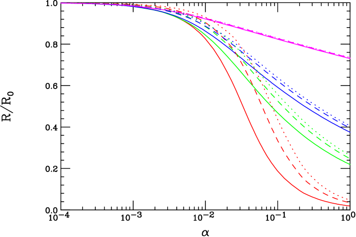
Figure 1: Influence of $\alpha\neq 0$ on the BH mass-Schwarzschild radius relationship for $n=2,4,6$ and 20, corresponding to the red, green, blue and magenta sets of curves, respectively. The solid, dashed and dotted curves in each case correspond to $m=M_{BH}/M_{*}=2,5,8$, respectively. Here $\beta=\gamma=0$.

Knowing the Lovelock generalizations of all of these quantities we can now proceed with our analysis. We will see that significant departures from the expectations of the EH action are easily obtainable. While examining these various quantities it is important to recall that which BH properties are measurable within the ADD framework. As mentioned above, collider measurements of other ADD signatures will tell us the values of $n$ and $M_{*}$[2], while the BH mass itself can be determined by direct reconstruction[21, 22]; similarly the cross section, i.e., $R$ can be obtained directly. Given $M_{BH},n$ and $M_{*}$, various BH decay distributions will help to determine other quantities such as the temperature[21, 22]. Measurement of the average multiplicity in the BH decay can give us a handle on the BH temperature as $<N>\simeq m/2T$[8] (before fragmentation effects are included). Of course, quantities such as the entropy and free energy are not directly measurable but are of theoretical interest. The specific heat of the BH can be inferred in some cases as it is indirectly probed by the BH lifetime. As we will see below, in contrast to the usual EH scenario, the BH may now have a positive specific heat making it grow cooler as it sheds mass via Hawking radiation. In such a case the BH may have a long lifetime.

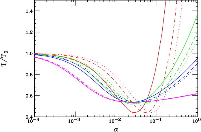
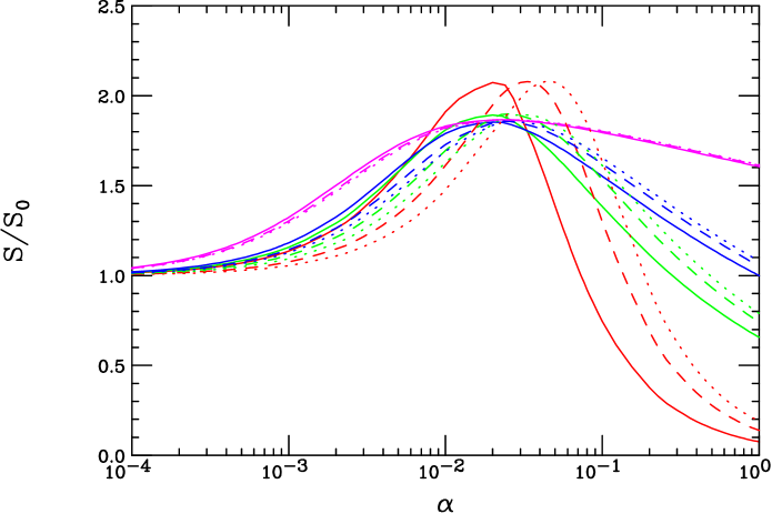
Figure 2: Same as in the previous figure but now for the BH temperature(top) and entropy(bottom).

3 Analysis

Given the generalized expressions above we can now ask how much of a numerical influence the Lovelock invariants will have on the quantities of interest. The first issue to address is the values of the parameters $\alpha,\beta$ and $\gamma$. As a first guess one might naively expect these to be of order unity. However, if we think of the Lovelock terms as arising from a perturbative-like expansion of the full action, as in string theory, the coefficients must grow smaller for the higher order Lovelock terms. Also, when we examine the expressions above we see that for any kind of perturbative expansion to make sense we must have, at least approximately, $\alpha n^{2},\beta n^{4}$ and $\gamma n^{6}<1$. Since $n$ can be as large as 6 within the usual ADD scenario, very crudely, we might expect that $\alpha\sim 10^{-2}$, $\beta\sim 10^{-3}-10^{-4}$ and $\gamma\sim 10^{-5}$ with a wide margin allowed for errors in these estimates. Since our arguments point to potentially different values of interest, in what follows we will allow for significant ranges of these Lovelock parameters.

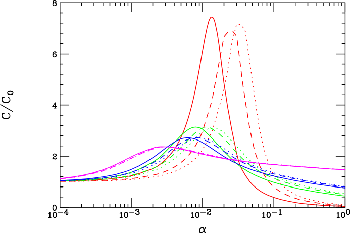
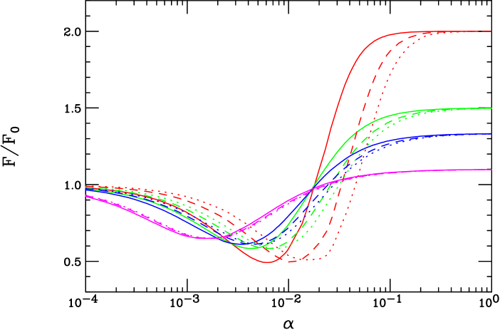
Figure 3: Same as in the previous figure but now for the BH heat capacity(top) and free energy(bottom).

In order to simplify our analysis of the influence of the various Lovelock invariants it is perhaps best to examine them one at a time; we first set $\beta=\gamma=0$ and consider the case of $\alpha\neq 0$. This is the most familiar possibility corresponding to Gauss-Bonnet gravity discussed in the literature [23, 24]. In order to elucidate the effects of $\alpha\neq 0$ for any fixed value of $n$ and $M_{BH}$ it is useful to scale out the results by the predictions of the usual EH action as can be done using the expressions above. As we will see the various quantities of interest will have a reasonably simple dependence on $\alpha$ for fixed values of $m=M_{BH}/M_{*}$. For example, in the specific case of the Schwarzschild radius we will examine the ratio $R/R_{0}$ to which we now turn and which is displayed in Fig. 1. Here we see that the effect of a non-zero $\alpha$ on $R$ is rather mild for all values of $n$ unless $\alpha$ is larger than $\sim 10^{-2}$. Interestingly, on the right hand side of the plot we see that the cases with larger values of $n$ appear to be significantly less influenced by a non-zero $\alpha$ than do those with smaller $n$. These variations in $R$ can lead to significant modifications to the anticipated BH cross section. For example, if $\alpha\simeq 1$ and $n=2(6)$ the BH production cross section, $\sim R^{2}$, would be reduced by more than a factor of 100(5) due to the presence of this new Lovelock in the action in comparison to EH expectations.

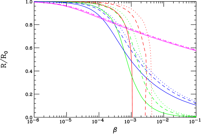
Figure 4: Same as Fig.1 but now as a function of $\beta$ with $\alpha=\gamma=0$ and $n=2\rightarrow n=3$ since ${\cal L}_{3}$ vanishes when $n=2$.

Fig. 2 shows the corresponding results for the temperature and entropy ratios, $T/T_{0}$ and $S/S_{0}$, as functions of $\alpha$. The results shown in these two plots appear to be reasonably (anti-)correlated as a result of of the entropy definition, Eq.(15). In the top panel we see that $T/T_{0}$ initially decreases as $\alpha$ increases, then goes through a minimum near $\alpha\sim 0.03-0.08$, then increases with a rapidity which is highly $n$ dependent. We see that as $n$ increases the steepness of this temperature rise rapidly decreases. Again, larger $n$ appear to be less sensitive to appreciable values of $\alpha$. The reverse behavior is seen in the case of the entropy variation with both $\alpha$ and $n$. Note that in both cases the ratios never differ from unity by more than factors of a few unless $\alpha$ becomes quite large. Thus, qualitatively, these BH are not too dissimilar from those of EH except for extreme choices of the parameter $\alpha$.

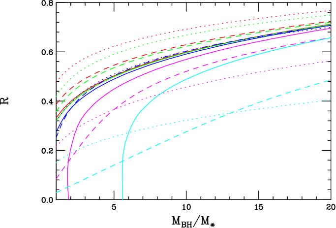
Figure 5: BH mass dependence of the Schwarzschild radius for the case $\alpha=\gamma=0$. Solid(dashed,dotted) curves correspond to $n=3(4,6)$, respectively. The red(green,blue,magenta,cyan) curves correspond to $\beta=0.00003(0.0001,0.0003,0.001,0.003)$, respectively. Note here that $R$ is in units of $M_{*}^{-1}$.

In Fig. 3 we see the behavior of both the heat capacity and free energy ratios with variations in $\alpha$. The values of these two quantities are reasonably simple and qualitatively similar to both $T$ and $S$. $F/F_{0}$ has an easily understandable behavior with increasing $\alpha$ since $F=m-TS$ and given the behavior above of the ratios $T/T_{0}$ and $S/S_{0}$. It is interesting to note that at large $\alpha$ the ratio $F/F_{0}$ asymptotes to a set of values which depend on $n$ and not $m$. As in the EH case, $\partial F/\partial m$ can be shown to be always positive and the heat capacity for BH is seen to be well behaved and is always negative as in the EH case. Thus BH with only non-zero $\alpha$ will Hawking radiate, evaporating completely or until a Planck-scale remnant stage is reached. For very large values of $\alpha\sim 1$, the mass loss through evaporation may be somewhat slowed in comparison to the usual EH case since the BH heat capacity, $\partial m/\partial T$, is so small. From Figs. 1-3, however, it is generally apparent that when $n\geq 2$ and only $\alpha$ is non-zero the typical BH will behave in a manner which is qualitatively similar to (though quantitatively different from) those that arise solely from the EH action. They are all unstable and will have relatively short lifetimes typical of more familiar hadronic processes.

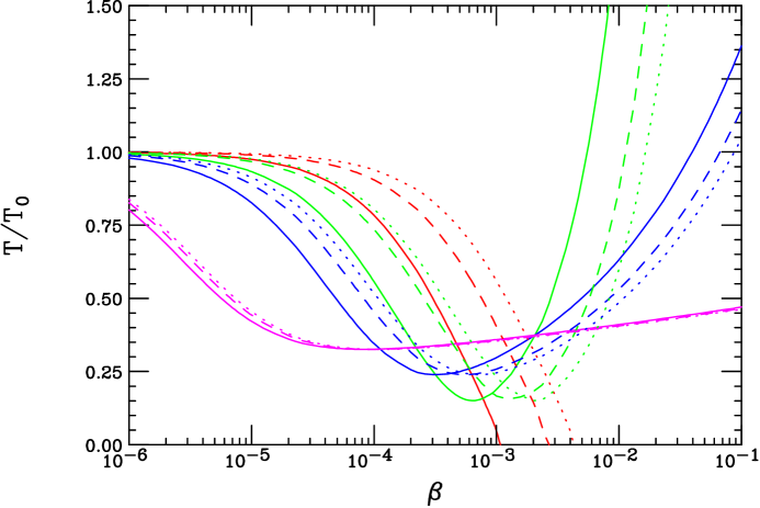
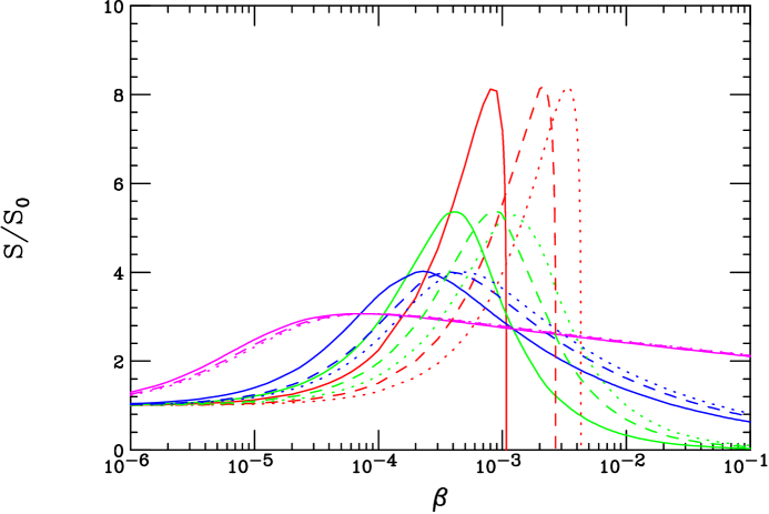
Figure 6: Same as Fig.2 but now as a function of $\beta$ with $\alpha=\gamma=0$ and with $n=2\rightarrow n=3$.

The behavior of BH properties with non-zero $\beta$ can be significantly different than what happens in the case of non-zero $\alpha$ as we will now see. (For simplicity we will assume $\alpha=\gamma=0$ while studying non-zero $\beta$; we note, however, that the behavior of non-zero $\gamma$ is qualitatively similar to non-zero $\beta$.) We can see this as soon as we examine the $\beta$ dependence of the ratio $R/R_{0}$ as is shown in Ref. 4. For small values of $\beta$ we see that the ratio $R/R_{0}$ decreases away from unity with smaller values of $n$ most seriously affected. This is quite similar to what we saw happen in the the case of non-zero $\alpha$. Clearly either large $\alpha$ or large $\beta$ can lead to a significant suppression of the BH production cross section; the same will be true of non-zero $\gamma$. Here, however, we see something new for the case $n=3$: the ratio $R/R_{0}\rightarrow 0$ for finite $\beta$. Turning this around, this means that for $n=3$ a non-zero $\beta$ implies that an horizon will not form unless $m$ exceeds a certain critical value, i.e., a BH will not form unless a certain mass threshold is reached. (Such a possible behavior has already been observed within the general context of Lovelock extended actions[23, 24]). This threshold effect can be seen analytically from Eq.(10) by setting $n=3$ with $\alpha=\gamma=0$ which yields the simple relation

$$m=c(x^{4}+24\beta)\,,$$ (20)

where here $c=5\pi^{3}/2$ and which is trivial to invert analytically to

$$x=\Big{[}{m\over{c}}-24\beta\Big{]}^{1/4}\,.$$ (21)

Here we see that unless $m>60\pi^{3}\beta$ there is no horizon. Note that for $\beta=5\cdot 10^{-4}$, a typical value, this means that unless $m>0.93$ no BH are formed. It is important to observe that a similar result is not obtainable when $n>3$; the case $n=3$ is therefore special when $\beta\neq 0$. Note that for fixed $\beta$ simultaneously turning on a non-zero $\alpha$ will lead to this same qualitative behavior with the same minimum value of $m$. Perhaps even more interesting is the fact that something almost identical happens in the case of non-zero $\gamma$ when $n=5$.

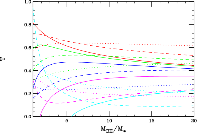
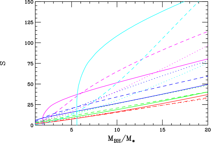
Figure 7: Same as Fig. 5 but now for the BH temperature and entropy with $n=2\rightarrow n=3$ as above. Note that here the temperature is in units of $M_{*}$.

This horizon threshold effect for non-zero values of $\beta$ can perhaps be best seen in Fig. 5 where we show $R$ as a function of $m=M_{BH}/M_{*}$. Here it is quite evident that there is a finite horizon threshold for the case $n=3$ while none exists for other $n$ values, i.e., $R\rightarrow 0$ when $m\rightarrow 0$. For $n>3$ this is easily understood from Eq.10 as there we see that $m=0$ when $x=0$. It is interesting to note that this threshold effect is not too dissimilar from what may happen for a 4-d BH when a renormalization group running of Newton’s constant is employed[26] in order to approximate leading quantum corrections; such a threshold scenario can also be seen to occur in theories with a minimum length[27] and in loop quantum gravity[28], which may also be thought of as a quantum effect. It is interesting to note that this threshold phenomena occurs in all these models where one tries to incorporate quantum corrections in some way; it would be interesting to learn whether or not this is a general feature of all such models.

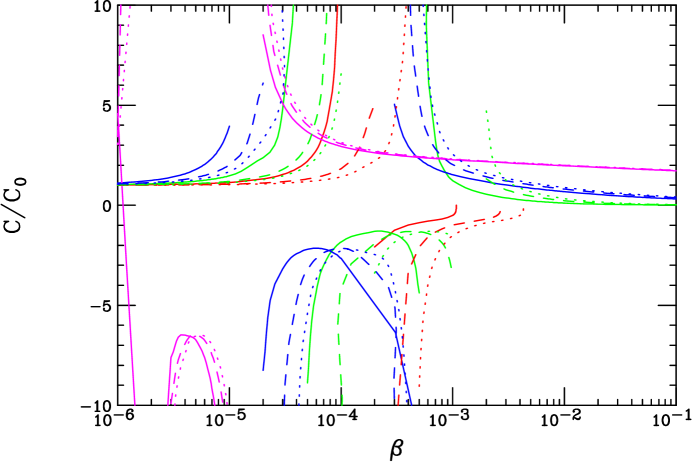
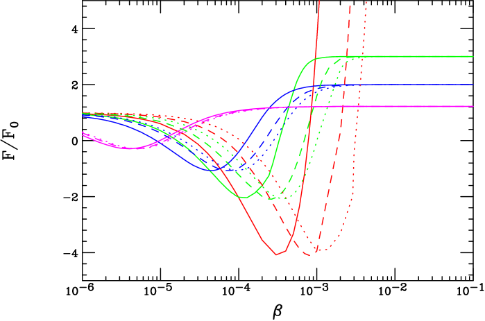
Figure 8: Same as Fig.3 but now as a function of $\beta$ with $\alpha=\gamma=0$.

We might expect that this unusual threshold-type behavior will have a significant influence on thermodynamic quantities. Fig. 6 shows the dependence of $T/T_{0}$ and $S/S_{0}$ as functions of $\beta$ for different values of $n$ and $m$. For $n>3$ this behavior is not so qualitatively different than that seen in the case of a non-zero $\alpha$ which is consistent with what was observed in Figs. 4 and  5. However, in Fig. 6 we see that for $n=3$ both the temperature and entropy can vanish. These zeros occur precisely at the values at which $R\rightarrow 0$ for the $n=3$ case that we observed above: $T$, $S$ and $R$ all vanish at the same parameter space points. These zeros in both the temperature and entropy for finite $m$ are also observed for the case of $n=3$ in Fig. 7 but we also see something new for other values of $n$. While $\partial S/\partial m$ was always positive, it is possible for $\partial T/\partial m$ to change sign in the mass range of interest. In the EH case, as well as for the examples of non-zero $\alpha$ examined above, $\partial T/\partial m$ was always seen to be negative. In many cases for $\beta\neq 0$, $T(m)$ is first observed to rise, reach a maximum, then decrease as $m$ grows larger.

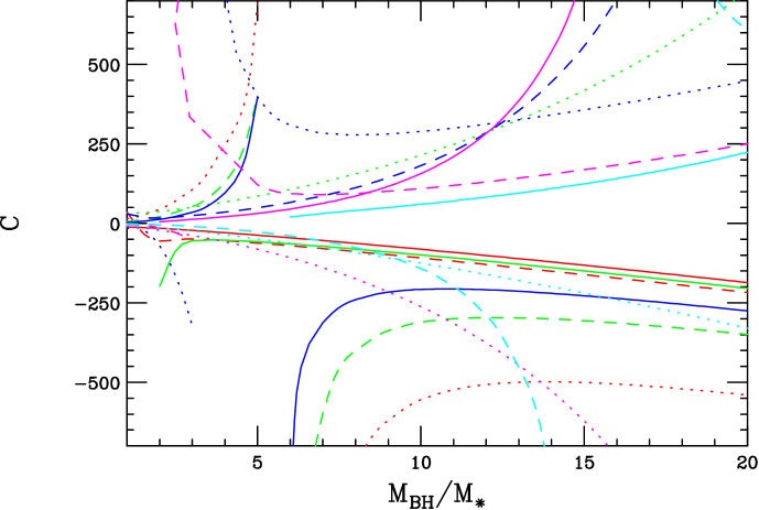
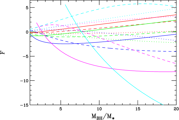
Figure 9: Same as the Fig.7 but now for the BH heat capacity and free energy. Recall that in our notation $F$ is units of $M_{*}$ while the heat capacity is dimensionless. Curves terminating (and not changing sign) in the middle of the plot correspond to locations where $R\rightarrow 0$.

To understand this more fully we turn to Figs. 8 and  9 which show the BH heat capacity and free energy both of which can now have rather complex behavior. The least unusual of the two is the ratio $F/F_{0}$, which apart from the case of $n=3$, is qualitatively similar to the that seen above for the case of a non-zero $\alpha$. However, we still see that $F$ can become negative for some values of $\beta$. On the otherhand, the specific heat/heat capacity is observed to have as many as two sign reversals associated with singularities in the parameter range of interest. In most cases $C/C_{0}$ is positive for both large and small $\beta$ with the reversals taking place at intermediate values. After some algebraic manipulations, it can be shown that for fixed values of $m$, $C(\beta)/C_{0}$ generally has two simple poles for real positive $\beta$ values. Such behavior is not unheard of for BH arising from Lovelock extended actions[23, 24] and may even occur in 4-d[29] for Kerr-Neumann BH. For the $n=3$ case, however, since the range of $R$ and $m$ is restricted there can be only one singularity.

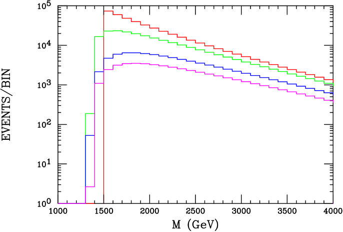
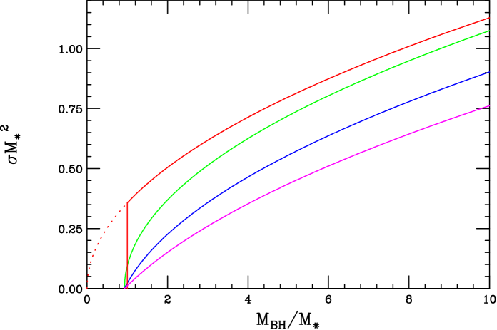
Figure 10: Threshold behavior of the BH cross section at the LHC(top) and ILC(bottom) for $n=3$. The red curve assumes the absence of Lovelock terms, while the green(blue,magenta) one corresponds to $\beta=0.0005$ with $\alpha=0(0.01,0.02)$. In the LHC case a luminosity(bin width) of 100 fb^-1 (100 GeV) has been assumed. In the ILC case a scaled cross section is presented as discussed in the text; the usual step-function turn on in the absence of Lovelock terms has been assumed. For the ILC $\sqrt{s}=M_{BH}$.

If we instead examine $C(m)$, as shown in Fig. 9, we see that there is at most one singularity corresponding to a simple pole in the physical region. For small $m$ we see that $C>0$ and then flips sign as $m$ increases above the singularity. This signals the existence of a kind of phase transition occurring at this singularity. $F(m)$ is also unusually behaved: in general it is positive for both small and large $m$ but goes through a negative minimum in between. Not unsurprisingly the location of the minimum in the free energy is the same as that of the singularity in the specific heat/heat capacity.

A parameter regime with positive heat capacity leads to interesting properties for BH. With only the EH action and thus a negative $C$, a BH loses mass via Hawking radiation; as it does so it get hotter thus radiating more quickly. This run-away process stops only when evaporation is complete or a non-classical Planck scale remnant is reached. Here, with $\beta\neq 0$, it is possible that the BH will end up in a mass regime where $C>0$ in which case it will get cooler as it gets lighter. Furthermore, there is a maximum temperature, given by the location of the pole in the heat capacity, for the BH. One might expect that such BH will live much longer than naively expected based on the EH action or even the combined EH+${\cal L}_{2}$ action. This is something completely new that happens when higher order Lovelock invariants are present. In some cases this may imply that the BH will become classically stable which is what happens in the case of $n=3$. To see this analytically, it is interesting to calculate the BH lifetime (in a vacuum!) directly assuming the semi-classical approach is viable. Recall that the amount of energy emitted by a black body per unit time is proportional to both its area and the fourth power of its temperature; using the results presented in Ref.[25] for $n=3$ with $\alpha=\gamma=0$ as an example we obtain

$${dm\over{dt}} \sim R^{2}T^{4}$$ (22)

$$\sim {{(m-60\pi^{3}\beta)^{7/2}}\over{(m+120\pi^{3}\beta)^{4}}}\,.$$

Integrating from some arbitrary initial mass, $m_{0}$, down to the threshold value, $60\pi^{3}\beta$ (where $T=0$), we obtain an infinite lifetime for all non-zero values of $\beta$. By ‘infinite lifetime’ we mean that it will take an infinitely long time for the mass of the BH to reach the threshold value. These mass thresholds may be identifiable with the anticipated Planck-scale remnant. We note that if $\beta=0$ a finite lifetime would be obtained. The addition of a non-zero value of $\alpha$ will not change this infinite lifetime result in a qualitative way. Thus any BH with a mass above the threshold value will decay by Hawking radiation quite rapidly losing most of its ‘excess’ mass until its mass approaches the threshold. Interestingly, we see from the figures that as the BH loses mass and approaches the threshold mass value from above the free energy approaches a minimum which is another indicator of classical stability. Of course, taking $\beta\rightarrow 0$ one recovers the finite lifetime that is usually expected on the basis of the EH action. This apparent BH stability is of course not unique to these particular parameter values; other BH do not lead to finite mass final states but may take an infinite time to evaporate completely. Furthermore, for $n=5$, we find that a similar situation is seen to occur when $\gamma$ is non-zero for arbitrary positive values of $\alpha,\beta$. Thus the so-called BH remnant in these cases can be uniquely identified with a BH with a mass very close to the threshold value.

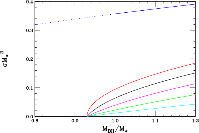
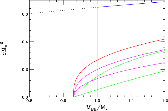
Figure 11: Close up of the BH production threshold at the ILC for $n=3$(top) and $n=5$(bottom); in these plots we should remember that $\sqrt{s}=M_{BH}$. The blue line in the naive $\theta$-function that is usually assumed in the absence of Lovelock terms. For the case $n=3$ with $\beta=0.0005$ the curves correspond to $\alpha=0,0.002,0.005,0.01$ and 0.02 from top to bottom, respectively. For the case $n=5$ all curves have $\gamma\simeq 1.14\cdot 10^{-5}$ and, from top to bottom, have $\alpha,\beta=0,0(0.003,0;0,0.00003;0.01,0;0,0.0001)$, respectively.

At this point it is important that the reader be reminded that even though we are trying to model quantum/stringy corrections via the Lovelock invariants, these are still semi-classical predictions which are subject to true quantum corrections that may modify them significantly. Though classically stable, these BH may have finite lifetimes due to these quantum corrections. It is possible, however, that these lifetimes will remain quite long.

4 A Toy Model of BH Collider Cross Section Thresholds

As discussed above, the usual picture of collider BH production is that there is a $\theta$ function-type threshold at $M_{*}$ which is certainly unphysical. Clearly quantum and/or stringy corrections will turn this step function behavior into something smooth which might be modeled via additional Lovelock terms in the action. If TeV scale extra dimensions exist and BH are produced at future colliders, the threshold region, where these effects are most relevant, will be important to understand in detail since it will provide a handle on the true underlying theory of quantum gravity. In the scenario we propose below, this corresponds to extracting the values of the Lovelock parameters by examining the nature of the cross section threshold. This is akin to using the nature of the threshold for new particle production to determine the particle’s spin and other quantum numbers.

The analysis in the previous section suggests a toy model that yields a more properly behaved threshold for BH production, at least in the cases $n=3(5)$, when $\beta(\gamma)$ is non-zero. There we saw that, e.g., a non-zero $\beta$ for $n=3$ implies the existence of a minimum mass below which a BH simply will not form. We also saw that this mechanism was absent for even values of $n$. For reasonable values of the Lovelock parameters what do these BH thresholds look like? Sticking with the case $n=3$ for now, let us take $\beta=0.0005$, in the center of the range discussed above with $\alpha$ set to zero for the moment for simplicity. Note that since $n=3$, $\gamma$ is automatically zero. The top panel in Fig. 10 shows what this would imply for the LHC BH (very large) production rate assuming that $M_{*}=1.5$ TeV for purposes of demonstration. First we notice the red histogram which is the usual $\theta$-function turn-on cross section prediction. The green histogram shows the same cross section but now with $\beta=0.0005$ and no $\theta$-function. There is clearly a threshold near 1.5 TeV but the turn-on is no longer infinitely sharp; for large BH masses we see that this prediction asymptotes to that of the naive $\theta$-function histogram. This result we may have expected since for large values of $M_{BH}$ we should recover the predictions associated with the EH action. Turning on non-zero but typical values of $\alpha\sim 0.01$ does not alter the threshold location but does modify the cross section shape near the threshold. Apparently the larger the value of $\alpha$ the softer the slope of the cross section near threshold. In fact a short analysis shows that the slope of the cross section goes as $\sim 1/\alpha$ precisely at the threshold. Of course, radiative corrections will smear out the fine details of these rather sharp threshold shapes. For non-zero $\alpha$ the cross section is seen to still asymptote to the naive value in the large $M_{BH}$ limit as it should.

Although a detailed simulation is far beyond the scope of the present work it is clear from the top panel in Fig. 10 that, while the LHC will observe the BH production threshold, an extraction of the Lovelock parameter values with any precision will be difficult. The bottom panel of this figure shows what may be seen at the ILC; here a set of scaled cross section results are presented so that the reader can move the threshold as they prefer. For example, if $M_{*}=1$ TeV, $\sigma M_{*}^{2}=1$ corresponds to a cross section of $\simeq 389.4$ pb; there will be no shortage of statistics. As in the case of the LHC the red curve is the naive step function turn-on while the other curves show the effect of the non-zero Lovelock parameters. To get a better idea of the ILC threshold region we zoom in using the top panel of Fig. 11. In this idealized picture we see that the step function curve is very far away from any of those produced by the Lovelock terms. The Lovelock cross section predictions are themselves rather widely separated from each other and have quite distinct shapes as they approach the threshold. Again, we recall that if $M_{*}=1$ TeV, a single vertical tickmark on this plot corresponds to a cross section change of $\sim 8$ pb, i.e., $\sim 10^{6}$ events at the ILC in one year. Of course in the real world this threshold region will be made more complex by both electroweak and gravitational radiative corrections that may smear out the threshold to some extent. Just how significant such effects will be is not yet known even within the very limited scope of the present toy model.

For the case of $n=5$ a non-zero $\gamma$ also induces a BH mass threshold and the bottom panel shows the corresponding cross sections assuming $\gamma\simeq 1.1\cdot 10^{-5}$, a value in the anticipated region discussed above. Note that the slope of the cross section in the threshold region is generally increased as $n$ increases. Turning on different values of $\alpha$ and $\beta$ again leads to detailed modifications of the threshold cross section shape. When $\alpha=\beta=0$, the slope of the cross section at threshold is infinite; a short analysis shows that in this case the slope behaves as $\sim 1/\beta$ near threshold and is independent of $\alpha$. The various curves are seen to be sufficiently different as to be likely distinguishable at the ILC even after radiative effects are included. Thus we see that the cases $\beta\neq 0$ and $\gamma\neq 0$ are qualitatively similar but are clearly separable once measurements with any precision become possible.

At least for the case of $n$ odd we see that the Lovelock invariants can lead to a reasonably smooth turn on of BH production in the mass range near $M_{*}$. The precise nature of this turn in is highly correlated with the various parameter values and the number of extra dimensions.

5 Conclusions

In this paper we have examined how the production of TeV-scale black holes at colliders is influenced by the existence of higher curvature Lovelock invariants in the action of models with large extra dimensions. This possibility is anticipated on rather general grounds when we try to embed such models in a larger theoretical structure, e.g., strings, if we also wish to maintain unitarity and freedom from ghosts. In the case of the ADD model, we argued that the addition of the Lovelock invariants to the Einstein-Hilbert action would leave the more conventional missing-energy and spin-2 contact interaction signatures unaltered but would modify the anticipated properties of TeV scale BH since the ADD geometry is essentially flat. These modifications in BH properties provide the only signature for the existence of higher curvature terms in this context. Since the total number of dimensions $D=4+n$ in string-motivated ADD is $\leq 10$ and the properties of the Lovelock invariants are highly restrictive, it was easily shown that at most three such terms, ${\cal L}_{2,3,4}$, can be added to the usual Einstein-Hilbert action. The strengths of these new interactions are described by a set of dimensionless parameters and, given the expectation that such terms result from some form of perturbative expansion, we derived some rough estimates for their anticipated magnitudes.

The next step in our analysis was to obtain the general expressions for the Schwarzschild radius, Hawking temperature, entropy, heat capacity/specific heat and free energy relevant for the $D$-dimensional TeV-scale BH in Lovelock gravity models with our specific generalized action. Using these results we then performed a detailed numerical investigation to probe the sensitivity of the BH production cross section as well as these thermodynamic quantities to variations in the values of the Lovelock parameters. Since the number of potentially contributing invariants is $n$-dependent, we examined the possibility of non-zero values for coefficients ($\alpha$ and $\beta$) of both ${\cal L}_{2,3}$ one at a time; while the impact of ${\cal L}_{2}$ and ${\cal L}_{3}$ were found to be quite distinct, ${\cal L}_{4}$ leads to results which are quite similar to ${\cal L}_{3}$ and so was not examined in detail.

For non-zero values of $\alpha$, up to factors or order unity, the BH thermodynamical properties are overall qualitatively similar to those found in the pure EH case except when $\alpha$ get very large. The BH Schwarzschild radius is, however, significantly smaller which suppresses the collider BH production cross section. When $\beta$ is non-zero, both quantitative as well as qualitative variations in the BH properties can be anticipated especially for the case of $n=3$; these variations from EH expectations can be somewhat exotic. We showed that they include sign changes in the heat capacity/specific heat, indicative of phase transitions, negative free energies and BH mass thresholds, i.e., mass values below which BH cannot form. In particular we observed that BH can now become thermodynamically stable, i.e., it would take an infinite time for them to Hawking radiate down to their threshold masses. This is correlated with BH now possibly having positive heat capacities so that they cool as they lose mass thus slowing the mass loss process itself.

We then demonstrated that for $n=3,5$ the minimum BH masses induced by the Lovelock invariants could be used as a toy model for the BH production cross section threshold. Instead of a step function turn-on, the cross section near threshold was shown to be highly sensitive to the values of $\alpha,\beta$ and $\gamma$ yet would still asymptote to that expected in the pure EH case. These differences would surely show up at the LHC and can be probed in detail at the ILC due to the large cross section and the enormous statistics available. It may be possible to use these BH mass thresholds to extract the values of the Lovelock parameters themselves.

TeV scale BH can provide a unique tool to probe the underlying theory of gravity. Hopefully they will be seen at future colliders.

Acknowledgments

The author would like to thank J.Hewett and B. Lillie for discussions related to this work.

References

- [1] N. Arkani-Hamed, S. Dimopoulos and G. R. Dvali, Phys. Rev. D 59, 086004 (1999) [arXiv:hep-ph/9807344] and Phys. Lett. B 429, 263 (1998) [arXiv:hep-ph/9803315]; I. Antoniadis, N. Arkani-Hamed, S. Dimopoulos and G. R. Dvali, Phys. Lett. B 436, 257 (1998) [arXiv:hep-ph/9804398].
- [2] J. Hewett and M. Spiropulu, Ann. Rev. Nucl. Part. Sci. 52, 397 (2002) [arXiv:hep-ph/0205106].
- [3] G. F. Giudice, R. Rattazzi and J. D. Wells, Nucl. Phys. B 544, 3 (1999) [arXiv:hep-ph/9811291].
- [4] T. Han, J. D. Lykken and R. J. Zhang, Phys. Rev. D 59, 105006 (1999) [arXiv:hep-ph/9811350].
- [5] E. A. Mirabelli, M. Perelstein and M. E. Peskin, Phys. Rev. Lett. 82, 2236 (1999) [arXiv:hep-ph/9811337].
- [6] J. L. Hewett, Phys. Rev. Lett. 82, 4765 (1999) [arXiv:hep-ph/9811356].
- [7] T. Banks and W. Fischler, hep-th/9906038.
- [8] S. Dimopoulos and G. Landsberg, Phys. Rev. Lett. 87, 161602 (2001) [arXiv:hep-ph/0106295].
- [9] S. B. Giddings and S. Thomas, Phys. Rev. D 65, 056010 (2002) [arXiv:hep-ph/0106219].
- [10] For a recent review, see P. Kanti, arXiv:hep-ph/0402168.
- [11] B. Zwiebach, Phys. Lett. B 156, 315 (1985). See also D. G. Boulware and S. Deser, Phys. Rev. Lett. 55, 2656 (1985) and B. Zumino, Phys. Rept. 137, 109 (1986).
- [12] N. E. Mavromatos and J. Rizos, Phys. Rev. D 62, 124004 (2000) [arXiv:hep-th/0008074].
- [13] D.Lovelock, J. Math. Phys.12, 498 (1971) . See also C. Lanczos, Z. Phys. 73, 147 (1932) and Ann. Math. 39, 842 (1938).
- [14] L. Randall and R. Sundrum, Phys. Rev. Lett. 83, 3370 (1999)
- [15] See, for example, T. G. Rizzo, arXiv:hep-ph/0412087, and references therein.
- [16] F. Mueller-Hoissen, Phys. Lett. B 163, 106 (1985).
- [17] C. C. Briggs, arXiv:gr-qc/9703074.
- [18] L. A. Anchordoqui, J. L. Feng, H. Goldberg and A. D. Shapere, Phys. Rev. D 66, 103002 (2002) [arXiv:hep-ph/0207139].
- [19] S. B. Giddings and V. S. Rychkov, arXiv:hep-th/0409131.
- [20] V. S. Rychkov, arXiv:hep-th/0410041; H. Yoshino and V. S. Rychkov, arXiv:hep-th/0503171.
- [21] C. M. Harris, M. J. Palmer, M. A. Parker, P. Richardson, A. Sabetfakhri and B. R. Webber, arXiv:hep-ph/0411022.
- [22] J. Tanaka, T. Yamamura, S. Asai and J. Kanzaki, arXiv:hep-ph/0411095.
- [23] J. T. Wheeler, Nucl. Phys. B 273, 732 (1986) and Nucl. Phys. B 268, 737 (1986). See also, B. Whitt, Phys. Rev. D 38, 3000 (1988); D. L. Wiltshire, Phys. Lett. B 169, 36 (1986) and Phys. Rev. D 38, 2445 (1988).
- [24] There is a vast literature on this subject. For a far from exhaustive list see, for example, R. G. Cai, Phys. Rev. D 65, 084014 (2002) [arXiv:hep-th/0109133], Phys. Lett. B 582, 237 (2004) [arXiv:hep-th/0311240] and Phys. Rev. D 63, 124018 (2001) [arXiv:hep-th/0102113]; R. C. Myers and J. Z. Simon, Phys. Rev. D 38, 2434 (1988); S. Nojiri, S. D. Odintsov and S. Ogushi, Phys. Rev. D 65, 023521 (2002) [arXiv:hep-th/0108172]; Y. M. Cho and I. P. Neupane, Int. J. Mod. Phys. A 18, 2703 (2003) [arXiv:hep-th/0112227] and Phys. Rev. D 66, 024044 (2002) [arXiv:hep-th/0202140]; T. Clunan, S. F. Ross and D. J. Smith, Class. Quant. Grav. 21, 3447 (2004) [arXiv:gr-qc/0402044]; R. G. Cai and Q. Guo, Phys. Rev. D 69, 104025 (2004) [arXiv:hep-th/0311020]; N. Okuyama and J. i. Koga, arXiv:hep-th/0501044; J. Crisostomo, R. Troncoso and J. Zanelli, Phys. Rev. D 62, 084013 (2000) [arXiv:hep-th/0003271]; M. Cvetic, S. Nojiri and S. D. Odintsov, Nucl. Phys. B 628, 295 (2002) [arXiv:hep-th/0112045]; R. Aros, R. Troncoso and J. Zanelli, Phys. Rev. D 63, 084015 (2001) [arXiv:hep-th/0011097]; E. Abdalla and L. A. Correa-Borbonet, Phys. Rev. D 65, 124011 (2002) [arXiv:hep-th/0109129]; T. Jacobson, G. Kang and R. C. Myers, Phys. Rev. D 52, 3518 (1995) [arXiv:gr-qc/9503020] and Phys. Rev. D 49, 6587 (1994) [arXiv:gr-qc/9312023]; T. Jacobson and R. C. Myers, Phys. Rev. Lett. 70, 3684 (1993) [arXiv:hep-th/9305016]; S. Deser and B. Tekin, Phys. Rev. D 67, 084009 (2003) [arXiv:hep-th/0212292].
- [25] See however, A. Barrau, J. Grain and S. O. Alexeyev, Phys. Lett. B 584, 114 (2004) [arXiv:hep-ph/0311238].
- [26] A. Bonanno and M. Reuter, Phys. Rev. D 62, 043008 (2000) [arXiv:hep-th/0002196].
- [27] See M. Cavaglia, S. Das and R. Maartens, Class. Quant. Grav. 20, L205 (2003) [arXiv:hep-ph/0305223] and references therein.
- [28] M. Bojowald, R. Goswami, R. Maartens and P. Singh, gr-qc/0503041.
- [29] See, for example, C. O. Lousto, Int. J. Mod. Phys. D 6, 575 (1997) [arXiv:gr-qc/9601006] and references therein.