Phenomenology Beyond the Standard Model

Abstract

An elementary review of models and phenomenology for physics beyond the Standard Model (excluding supersymmetry). The emphasis is on LHC physics. Based upon a talk given at the Physics at LHC conference, Vienna, 13-17 July 2004.

1 Causarum Investigatio

Written on the ceiling fresco of the beautiful Festsaal of the Österreichischen Akademie der Wissenschaften, are two words: Causarum Investigatio. Just as these words must have inspired Boltzmann and Schrödinger, today we are inspired to investigate the causes and more fundamental structures underlying the Standard Model of particle physics.

The Standard Model is in remarkably successful agreement with particle physics data at all energies below the scale of electroweak symmetry breaking. Indirect probes of physics up to multi-TeV scales, using rare decays, or using the sensitivity of electroweak precision data to virtual processes, also show no significant deviations. Thus, in a strict experimental sense, we have no guidance for moving beyond the Standard Model, other than the clear anomalies of neutrinos oscillations, dark matter, and dark energy.

Figure 1: The big picture of physics beyond the Standard Model.

However, the success of the Standard Model indicates that fundamental physics is closely tied to the basic principles of quantum mechanics and to symmetry principles, of which the most notable are relativity and local gauge invariance. These provide a very constrained set of rules for extensions of the Standard Model, and a great deal of theoretical investigation in the past twenty five years has been devoted to mapping out the possible scenarios consistent with these rules.

Indeed, our theoretical understanding of these structures is now so mature that it is not overly pretentious to sketch the “big picture” of physics beyond the Standard Model. This sketch is illustrated in Figure 1, where the vertical direction represents energy scale. The two scales shown are: the “TeV” scale characterized by the new physics responsible for electroweak symmetry breaking, and the “string unification” scale, defined as the scale where one begins to have a unified description of quantum gravity with the gauge interactions of the Standard Model.

We know the TeV scale (within an order of magnitude), but we do not know what is the new physics responsible for electroweak symmetry breaking. Many very distinct and theoretically viable mechanisms have been proposed. Identifying and understanding this physics is the primary goal of the LHC project.

We do not know the scale of unification (even to within an order of magnitude) nor do we know to what extent it involves gauge coupling unification, grand unification, flavor unification, or superstrings. But our best guess is that some combination of all of these elements is involved. Determining this scale and uncovering the new physics in operation there is one of the ultimate goals of particle physics.

The figure also demonstrates another equally important and more immediate goal. If unification occurs in any form, then there must be highly sophisticated dynamical mechanisms which convert the simple unified theory at ultra high energies into the messy junk which we observe in experiments today. These are shown in the figure as the mechanisms which respectively break supersymmetry and hide extra dimensions. We do not understand either of these mechanisms, though again theorists have proposed many distinct possibilities. Determining which mechanisms Nature has chosen is a process we expect to begin at the LHC, and continue with future colliders.

Since supersymmetry (SUSY) is well-covered in other sessions at the conference [1], I will concentrate here on extra dimensions and related ideas. However I hasten to add that one should never regard supersymmetry and extra dimensions as mutually exclusive. On the contrary, it is extremely difficult to imagine that any of the current ambitious schemes with extra dimensions can stably devolve from the unification scale without the help of SUSY. It is only somewhat easier to imagine that the minimal picture of supersymmetric unification actually works, without at least some assistance near the high scale from an orthogonal organizing principle like extra dimensions. And we should not forget that string theory needs them both.

It is also true that there are many topics in Beyond the Standard Model (BSM) phenomenology which are neither SUSY nor extra dimensions. However this division has grown fuzzy of late. For example, almost all of the current theoretical research on models with new strong dynamics are exploiting the AdS/CFT correspondence to map these gauge theories into models of extra dimensions with branes. Thus while our review contains no mention of technicolor, I will discuss recent work on “Higgsless” models in extra dimensions [2]. Similarly much of the increase in our understanding of strongly coupled gauge theories during the past decade has come from the study of SUSY gauge theories, and this has begun to be reflected in BSM model-building. Thus for example the recent “fat Higgs” models [3] modify the conventional SUSY desert scenario via an elegant matching of two gauge theories while preserving gauge coupling unification. This has the attractive feature of solving the post-LEP “little hierarchy” problem, and at the very least is a counterexample to arguments which purport to demonstrate the unique attractiveness of the minimal SUSY scenario.

Similarly, what used to be called “excited fermions” in BSM search talks now appear as ur-Kaluza-Klein modes in generic models of deconstruction. Leptoquarks, another old warhorse of BSM searches, will be discussed later in this review. I will show how leptoquarks can most profitably be regarded as products of either SUSY or extra dimensions.

Having thus dramatically shortened the usual laundry list for BSM reviews, I end the introduction with an additional disclosure. This review will be completely collider-centric. This is a clear deficiency, especially in an era where the interconnectedness of high energy physics and astrophysics plays an absolutely essential role. As already mentioned, the only clear deviations from the Standard Model to date are neutrino oscillations, dark matter, and dark energy. None of these were discovered at colliders. In the future, I expect that studies of rare processes, B physics, the neutrino sector, cosmology, particle astrophysics, and particle astronomy will all provide important clues to BSM physics. However I also expect collider experiments to be the major contributors to reaching the ambitious goals which I have outlined above.

2 A bestiary of extra dimensions models

BSM review talks 15 years ago usually made no mention at all of extra dimensions. Since all of the reasons for taking extra dimensions seriously existed 15 years ago, this was a purely sociological absence, i.e., extra dimensions were not socially acceptable. This is perhaps a residual effect of the curse of Gunnar Nordström, the Finnish physicist who invented Kaluza-Klein theory in 1914, only to have his brilliant idea completely ignored by Einstein. Kaluza-Klein theory was, in turn, ignored by almost all physicists for a half century, finally being resuscitated by purveyors of supergravity and superstrings and the 1970s and 80s.

Briefly, there are three strong motivations for attempting to incorporate extra dimensions in BSM physics. The first motivation is the Standard Model (SM) itself, which has too many elementary particles (57 not including the Higgs) for a theory of fundamental constituents. Especially when one factors in the enormously complex flavor structure of the SM, it is clear that new dynamics is at work here, involving new degrees of freedom intimately connected to the SM degrees of freedom. New gauge interactions with resulting composites may be part of the answer, but probably not all of it. This leaves only two other known directions: extra dimensions, which when dynamically compactified or otherwise hidden create complex low energy patterns, and extended objects, which leads to string theory. String theory is itself the second prime motivation for extra dimensions, since quantized strings do not give reasonable physics unless they are embedded into a ten-dimensional spacetime. The third motivation is quantum gravity, broadly defined, which tells us that space and time are to be regarded as themselves fully “dynamical” objects. While it is not clear exactly what this means, it certainly implies that the number of accessible spatial dimensions at a given energy scale should be regarded as a dynamical physical observable, not given a priori.

Depending upon the physical mechanism invoked to hide extra dimensions from current observation, there is a great range of possible energy or length scales at which they may begin to appear. The most conservative guess is that their inverse radii are within about an order of magnitude of the unification scale; even in this case extra dimensions can have very significant effects upon physical observables at the TeV scale. In many models, the extra dimensions themselves appear around the TeV scale, and are linked to TeV scale physics such as electroweak symmetry breaking (EWSB) or supersymmetry breaking. In models which employ very efficient brane methods for hiding extra dimensions, the extra dimensions can even be of macroscopic size without contradicting any current observations or experiments. Indeed an extra dimension of infinite extent is not necessarily excluded.

A complete bestiary of extra dimensions models is beyond the scope of this review. We can make a partial survey based upon a simple organizing principle: what is the physical mechanism which hides the extra dimensions? Possible answers include:

• The extra dimensions are compact and small. Examples include a circle, a sphere, a torus, a Calabi-Yau manifold, and various kinds of orbifolds.

• Some or all of the SM particles are confined to a brane or an intersection of branes, and thus cannot probe the full extra dimensional “bulk” space.

• The extra dimensions are fundamentally different. For example, if the extra dimensions are fermionic, we are back to supersymmetry. The extra dimensions might also be discrete or otherwise “deconstructed”, so that they only approximately resemble spatial degrees of freedom in a certain energy regime.

• Any combination of the above.

In addition, it is important to specify whether the extra dimensions are curved or flat, and whether the various bulk fields have nontrivial vacuum configurations in the extra dimensions.

A glance at SPIRES reveals that there are in excess of 3,000 papers discussing extra dimensions models which fit into the above categorization. I can summarize the current status of these extra dimensions models in two bullets:

• There are too many models.

• None of them are any good.

The first bullet is obvious to any experimenter interested in searching for signals of extra dimensions at the LHC. What models should we simulate? What are the key phenomenological features and key discriminators between different models? These are basic questions which need to be answered before LHC turn-on.

The second bullet brings up some points which further complicate our task. Most of the work on extra dimensions is at the level which Savas Dimopoulos aptly calls “scenarios” rather than models. A scenario is defined (by me) as a set of physical assumptions which, with considerably more work, could evolve into a respectable class of models. Many of these scenarios have remained scenarios because they suffer from deep theoretical problems or “gaps”, and some of them have fairly nasty (but generic) phenomenological problems. This is not a reason to denigrate these scenarios – after all the same could be said of supersymmetry models or of string theory! But it does explain why we are still some way from having a decent set of serious and “theoretically stable” benchmark models for simulation.

That said, I will review the status of three out of the four classes of extra dimensions scenarios which are are most relevant for LHC searches. The fourth class, direct compactifications of string theory, is potentially the most interesting, but as of 2004 was not quite ready to make contact with LHC physics [4]-[9].

3 UED

Universal Extra Dimensions is the name given by Appelquist, Cheng, and Dobrescu [10] to a class of models which closely resemble the original Nordström-Kaluza-Klein scenario, but with some crucial improvements. All particles live in the full bulk, which is compactified to some kind of orbifold. The simplest case is a single extra dimension with coordinate $y$, compactified to a circle, which in turn is orbifolded to a line interval of length $L$ by identifying points under $y\to-y$. The orbifolding is necessary because otherwise the Kaluza-Klein zero modes of fermions (i.e. the light 4d fermions) are vectorlike. The orbifold projections in the above example remove half of the chiralities for the fermion zero modes, allowing an effective 4d theory which matches the chiral Standard Model.

These same orbifold projections have other good effects. For example, consider a 5-dimensional bulk gauge field $A_{M}=(A_{\mu},A_{y})$, where $\mu$ is a 4d vector label and $y$ labels the fifth dimension. Since $A_{y}$ appears in a 5d covariant derivative with $d/dy$, we keep the odd Kaluza-Klein (KK) modes of $A_{y}$ after orbifolding, while keeping the even KK modes of the $A_{\mu}$. This means that $A_{\mu}$ has a massless zero mode, but $A_{y}$ does not. Thus we manage to avoid having a massless adjoint scalar accompany every massless gauge boson in the effective 4d theory.

In the original Kaluza-Klein model Kaluza-Klein mode number is conserved, as this is just conservation of (discrete) momentum in the extra dimension. However in our simple UED example there are two orbifold fixed points: one is $y=0$ and the other is $y=L$. Thus orbifolding breaks the translational invariance of the circle, by distinguishing two special points. This may have no effect at tree level, but radiative corrections will generically introduce interactions which violate conservation of KK mode number. However a single remnant translation, $y\to y+L$, is still a symmetry, since it just interchanges the two fixed points. Since translation invariance is broken to a $\mathbf{Z_{2}}$ remnant, momentum conservation in the fifth dimension is replaced by a conserved parity, called “KK parity”. Zero modes are even under this parity but the lightest massive modes are odd.

This is enough to guarantee that the lightest massive KK mode in a UED model is stable. The situation is quite analogous to R parity in SUSY models. As with SUSY, this implies that in UED models the first massive KK modes must be produced in pairs. More generally, production of any single massive KK mode is quite suppressed, unless one introduces large tree level couplings which violate KK momentum conservation. This in turn suppresses the virtual corrections of these KK modes to Standard Model processes, allowing the UED scale $1/L$ to be as low as 300 GeV before we get into conflict with precision data. It also means that the lightest massive KK mode, the “LKP”, is a good cold dark matter candidate [11, 12].

Figure 2: Spectrum of the first massive KK modes of the Standard Model particles, in a simple UED model. Taken from reference [13].

UED models, in addition to being rather simple, have fairly universal predictions for colliders. If the LKP is a major constituent of dark matter, then it is in a mass-coupling range such that it will be produced at the LHC. Figure 2 shows a typical spectrum for the first massive KK modes in a UED model [13], after taking into account the mass splittings from radiative corrections. As in SUSY models the partner of the SM gauge boson $B$ tends to have the smallest radiatively corrected mass. The other first massive KK modes will decay promptly to this LKP. Thus typical UED events at the LHC give a variety of jet and lepton signatures combined with large missing transverse energy (MET).

If you only produce the first massive KK modes, UED models look very much like a subset of SUSY models, in terms of their collider signatures. Even if you detect a few of the second level KK modes, it is not obvious that this will dramatically disambiguate the signatures from an extended SUSY model; this should be studied. The crucial discriminators, of course, are the spins of the heavy partner particles. Distinguishing these spins is a very significant experimental challenge [14].

If we are lucky and the UED scale is close to the current bound, i.e. $1/L\sim 300$ GeV, then it will be possible to see UED effects as mimimal flavor violating loops in heavy flavor physics [15].

4 ADD

ADD is the name I use to refer to the class of models which incorporate the large extra dimensions scenario of Arkani-Hamed, Dvali, and Dimopoulos [16]. These were the first extra dimensions models in which the compactified dimensions can be of macroscopic size, consistent with all current experiments and observations. For this reason they are sometimes known as “large extra dimensions” models.

In the most basic version, $n$ extra spatial dimensions are compactified on a torus with common circumference $R$, and a brane is introduced which extends only in the three infinite spatial directions. Strictly speaking, the brane should have a very small tension (energy per unit volume) in order that it does not significantly warp the extra dimensional space. It is assumed that all of the SM fields extend only in the brane. This can be considered as a toy version of what happens in string theory, where chiral gauge theories similar to the SM are confined to reasonably simple brane configurations in reasonably simple string compactifications [17].

An immediate consequence of these assumptions is that the effective 4d Planck scale is related to the underlying fundamental Planck scale of the $4$$+$$n$-dimensional theory and to the volume of the compactified space. This relation follows immediately from Gauss’ Law, or by dimensional truncation:

$$M_{\rm Planck}^{2}=M_{*}^{2+n}\,R^{n}\quad,$$ (1)

where $M_{\rm Planck}^{2}$ is defined by Newton’s constant: $M_{\rm Planck}=1/\sqrt{G_{N}}=1.2\times 10^{19}$ GeV. $M_{*}^{2+n}$ is defined as the gravitational coupling which appears in the $4$$+$$n$-dimensional version of the Einstein-Hilbert action. It is the quantum gravity scale of the higher dimensional theory.

If $M_{\rm Planck}$, $M_{*}$ and $1/R$ are all of the same order, as is usually assumed in string theory, this relation is not very interesting. But there is nothing which prevents us from assuming that $M_{*}$ is equal to some completely different scale. Most attractive is to take $M_{*}\sim 1$ TeV, and attempt [18] to replace the hierarchy problem of the SM by a large compactification radius, i.e. to swap an ultraviolet problem for an infrared one! Note that, if we want to mantain contact with string theory, ADD-like models must arise from string ground states in which the string scale (and thus the ultraviolet cutoff for gravity) is also in the TeV range. This is difficult but not unthinkable [19].

The ADD scenario raises the exciting possibility of observing quantum gravity at the LHC. In such models only the graviton, and possibly some non-SM exotics like the right-handed neutrino, probe the full bulk space. There is a Kaluza-Klein tower of graviton modes, where the massless mode is the standard 4d graviton, and the other KK modes are massive spin 2 particles which also couple to SM matter with gravitational strength.

Whereas bremstrahhlung of ordinary gravitons is a completely negligible effect at colliders, the total cross section to produce some massive KK graviton is volume enhanced, and thus effectively suppressed only by powers of $M_{*}$, not $M_{\rm Planck}$. From Eq. (1) one obtains:

$$\sigma\sim{1\over M_{\rm Planck}^{2}}(ER)^{n}\sim{1\over M_{*}^{2}}(EM_{*})^{n}\quad,$$ (2)

where $E$ is the characteristic energy of the subprocess.

For graviton phenomenology it is useful to replace the ADD parameter $M_{*}$ by other rescaled parameters. The two most useful choices are taken from the work of Giudice, Rattazzi and Wells (GRZ) [20], and Han, Lykken and Zhang (HLZ) [21]:

$$M_{*}^{n+2} = {S_{n-1}\over(2\pi)^{n}}M_{s}^{n+2}\;,$$ (3)

$$M_{*}^{n+2} = {8\pi\over(2\pi)^{n}}M_{D}^{n+2}\;,$$ (4)

where $M_{s}$ is the HLZ scale, $M_{D}$ is the GRW scale, and $S_{n-1}$ is the surface area of a unit $n$-sphere:

$$S_{n-1}={2\pi^{n/2}\over\Gamma({n/2})}\;.$$ (5)

Both notations are equivalent. To obtain a complete dictionary between ADD, GRZ and HLZ, one also needs to relate the ADD parameter $R$ to those used by the other authors: $R=R_{\rm HLZ}=2\pi R_{GRW}$, and take note of the different notations for Newton’s constant:

$$\kappa^{2}=16\pi G_{N}\;(\rm HLZ);\quad\bar{M}_{P}^{2}={1\over 8\pi G_{N}}\;(\rm GRW)\;.$$ (6)

A Kaluza-Klein (KK) graviton mode has a mass specified by an $n$-vector of integers $\vec{k}$:

$$m^{2}(\vec{k})={\vec{k}^{2}\over R_{\rm GRW}^{2}}\;.$$ (7)

Let $r=|\vec{k}|$. Then for large $r$ (as is always the relevant case for ADD phenomenology) the number of KK graviton states of a given polarization with $r\leq r_{\rm max}$ is given by the integral

$$S_{n-1}\int_{0}^{r_{\rm max}}dr\,r^{n-1} = {1\over n}S_{n-1}\;r_{\rm max}^{n}\;$$ (8)

$$= \int_{0}^{m_{\rm max}}\rho(m)\,dm\;,$$

where the KK density of states is

$$\rho(m)={m^{n-1}\over G_{N}M_{s}^{n+2}}\;.$$ (9)

We see that $M_{s}$ is the natural scaling parameter for KK graviton production. The density of states formulation can be applied to a much more general class of models than ADD, and can also include graviton wavefunction factors when the extra dimensions are not flat.

Consider now on-shell production of a KK graviton from a $pp$ or $p\bar{p}$ collision. To leading order this is a $2\rightarrow 2$ process with two massless partons in the initial state, plus a massive KK graviton and a massless parton in the final state. Let $p_{1}$, $p_{2}$ denote the 4-momenta of the initial state partons, $p_{3}$ the 4-momentum of the graviton, and $p_{4}$ the 4-momentum of the outgoing parton. The total cross section for any particular variety of partonic subprocess has the form

$$\sigma(1+2\rightarrow{\rm KK}+4)=\int dx_{1}dx_{2}\,f_{1}(x_{1},\hat{s})f_{2}(x_{2},\hat{s})\int d\hat{t}\int_{0}^{\sqrt{\hat{s}}}dm\,\rho(m)\,{d\sigma_{m}\over d\hat{t}}(\hat{s},\hat{t})\,,$$ (10)

where $f_{1}(x_{1},\hat{s})$, $f_{2}(x_{2},\hat{s})$ are the parton distribution functions (pdfs) for the intitial state partons, $\hat{s}=x_{1}x_{2}s=(p_{1}+p_{2})^{2}$ is the square of the total center of mass (cm) energy of the subprocess, and $\hat{t}=(p_{1}-p_{3})^{2}$ is the usual Mandelstam invariant. The formulae for $d\sigma_{m}/d\hat{t}$, the differential subprocess cross sections for KK gravitons of mass $m$, are given in equations 64-66 of GRW.

5 RS

Randall-Sundrum refers to a class of scenarios, also known as warped extra dimensions models, originated by Lisa Randall and Raman Sundrum [22, 23]. In these scenarios there is one extra spatial dimension, and the five-dimensional geometry is “warped” by the presence of one or more branes. The branes extend infinitely in the usual three spatial dimensions, but are sufficiently thin in the warped direction that their profiles are well-approximated by delta functions in the energy regime of interest. If we ignore fluctuations of the branes, we can always choose a “Gaussian Normal” coordinate system, such that the fifth dimension is labelled $y$ and the usual 4d spacetime by $x^{\mu}$. The action for such a theory contains, at a minimum, a 5d bulk gravity piece and 4d brane pieces. The bulk piece has the 5d Einstein-Hilbert action with gravitational coupling $M^{3}$, and a 5d cosmological constant $\Lambda$. The brane pieces are proportional to the brane tensions $V_{i}$, which may be positive or negative. These act as sources for 5d gravity, contributing to the 5d stress-energy terms proportional to

$$\sum_{i}V_{i}\delta(y-y_{i})$$ (11)

where the $y_{i}$ are the positions of the branes. Combined with a negative $\Lambda$, this results in a curved geometry, with a 5d metric of the form:

$$g_{\mu\nu}(x^{\rho},y)=a^{2}(y)\,{\tilde{g}}_{\mu\nu}(x^{\rho})\;,$$

$$g_{\mu y}=0\;,\quad g_{yy}=1\;,$$ (12)

where $a(y)$ is called the warp factor, $\tilde{g}$ is a 4d metric, and I have made a useful choice of coordinates. Warping refers to the fact that a 4d distance $d_{0}$ measured at $y=y_{0}$ is related to an analogous 4d distance $d_{1}$ measured at $y=y_{1}$ by $a(y_{0})d_{0}=a(y_{1})d_{1}$. Thus in Randall-Sundrum scenarios 4d length, time, energy and mass scales vary with $y$.

So far we are being completely general. However almost all collider physics phenomenology done with warped extra dimensions so far is based upon one very specific model, the original simple scenario called RSI. In this model the extra dimension is compactified to a circle of circumference $2L$, and then further orbifolded by identifying points related by $y\to-y$. Thus the fifth dimension consists of two periodically identified mirror copies of a curved 5d space extending from $y=0$ to $y=L$. It is assumed that there is a brane at $y=0$, with positive tension $V_{0}$; it is known as the Planck brane. There is another brane at $y=L$, with negative tension $V_{L}$, known as the TeV brane.

Randall and Sundrum showed that, for a specially tuned choice of input parameters $V_{0}=-V_{L}=-M^{2}\Lambda$, the 5d Einstein equations have a simple warped solution on $0<y<L$ with metric:

$$g_{\mu\nu}(x^{\rho},y)={\rm e}^{-2ky}\,\eta_{\mu\nu}\;,$$

$$g_{\mu y}=0\;,\quad g_{yy}=1\;,$$ (13)

where $\eta_{\mu\nu}$ is the 4d flat Minkowski metric, and $k=\sqrt{-\Lambda}$. Away from the branes, the 5d curvature is constant and negative; it is thus equivalent locally to $AdS_{5}$, with the Anti-de Sitter radius of curvature given by $1/k$. At the locations of the branes the curvature is discontinuous, due to the fact that the branes are delta function sources for curvature.

We see that the RSI model is completely described by three parameters: $k$, $M$, and $L$. Since we are not resolving the brane profiles, and since we do not want to worry about how to embed this scenario into string theory or some other description of quantum gravity, we had better restrict ourselves to a low energy effective description. This implies taking $k$, $1/L\ll M$. In fact in RSI it is assumed that $k$ is merely parametrically small compared to the 5d Planck scale $M$, i.e. something like $k\sim M/10$. The effective 4d Planck scale, which is the same thing as the coupling of the graviton zero mode, is given by dimensional truncation:

$$M_{\rm Planck}={M^{3}\over 2k}\left(1-{\rm e}^{-2kL}\right)\;.$$ (14)

Thus, within an order of magnitude, $M\sim k\sim M_{\rm Planck}$. In RSI we fix the distance $L$ by requiring that $a(L)M_{\rm Planck}\simeq 1$ TeV, thus $kL\sim 30$. This is not a large extra dimension: its inverse size is comparable to the grand unification scale.

The RSI model makes one further simple but drastic assumption: that our entire 4d universe is confined to the TeV brane. From a particle physics viewpoint (and completely ignoring cosmology) this amounts to the statement that the Standard Model fields live on the TeV brane. Thus, as in ADD models, the phenomenology of RSI is concerned with the effects of the massive KK modes of the graviton. These modes are quite remarkable since, as measured on the TeV brane, their mass splittings are on the order of a TeV, and their couplings to SM fields are only TeV suppressed. In RSI, the Standard Model is replaced at the TeV scale by a new effective theory in which gravity is still very weak, but there are exotic heavy spin-two particles.

At the LHC the KK gravitons of RSI would be seen as difermion or diboson resonances, since (unlike the KK gravitons of ADD) the coupling of each KK mode is only TeV suppressed [24]. The width of these resonances is controlled by the ratio $k/M$; the resonances become more narrow as $k/M$ is reduced, as shown in Figure 3.

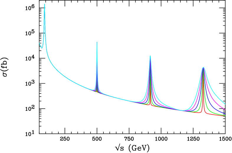
Figure 3: The cross section for $e^{+}e^{-}\to\mu^{+}\mu^{-}$ including the exchange of KK gravitons in the RSI model. The narrowest resonances correspond to $k/M=0.05$, the widest to $k/M=0.14$. Taken from reference [25].

6 A behaviorist approach to extra dimensions

The three wildly popular scenarios just reviewed are probably all too simplistic to stand as viable candidates for top-down theories of extra dimensions. But as already mentioned, our only viable top-down theory of extra dimensions, string theory, is not yet understood well enough to guide experiments at the LHC.

For collider phenomenology, we don’t care so much where the extra dimensions models came from; what we care about is what they do. This suggests a more bottom-up approach, where we don’t worry (much) about whether our models can be fleshed out into globally respectable theories. Instead, we focus on particular theoretical conundrums which can be solved by invoking extra dimensions. Then we ask what are the distinctive phenomenological features of each solution.

Here is a partial list of “solutions” to theoretical problems which have been suggested using extra dimensions (often in more than one way):

• explain or assist electroweak symmetry breaking

• explain the little hierarchy problem

• lower the Planck scale

• break supersymmetry

• explain flavor properties of the SM

• improve grand unification

• explain neutrino physics

• explain dark matter

• explain dark energy

I will briefly review three such phenomenologically oriented efforts: little Higgs, Higgsless models, and asymmetrical extra dimensions.

7 Deconstructing little Higgs

The SM is an effective field theory with a cutoff scale $\Lambda$. Since the Higgs has quadratically divergent radiative corrections at one loop, we expect that $\Lambda\sim(4\pi/g)*174$ GeV $\sim 1$ TeV. It is therefore surprising that precision collider tests, with multi-TeV sensitivity, see no evidence for any of the dimension 5 and 6 operators which can be constructed purely from Standard Model fields, obeying all SM symmetries. This is known as the little hierarchy problem, since taken at face value it suggests that the cutoff $\Lambda$ may be closer to 10 TeV than it is to 1 TeV.

Little Higgs models [26]-[36] address this problem by making the Higgs a pseudo-Goldstone boson of new global symmetries which are both explicitly broken (by SM gauge interactions) and spontaneously broken. Roughly speaking, this buys you another factor of $4\pi$ in the relation given above, allowing the cutoff $\Lambda$ to be naturally around 10 TeV.

Little Higgs model builders will claim that their models have nothing to do with extra dimensions, but as far as I know extra dimensions are the best motivation for this scenario.

Consider a 5d $SU(N)$ gauge theory. Force the extra dimension to be discrete, i.e. a finite periodic lattice with $m$ sites and lattice spacing $1/f$. The 5d Yang-Mills lagrangian then truncates to

$${1\over 2g^{2}}\sum_{i=1}^{m}{\rm tr}\,F_{i}^{2}+f^{2}\sum_{i=1}^{m}{\rm tr}\,\left[(D_{\mu}U_{i})^{\dagger}D^{\mu}U_{i}\right]\;.$$ (15)

For finite $m$ this is really a 4d theory, with $m$ different sets of $SU(N)$ gauge bosons, together with “link” scalars $U_{i}$ which are bifundamentals, i.e. they each carry charges under two different “adjoining” $SU(N)$’s. The $U_{i}$ are just the latticized versions of the $A_{y}$, the extra-dimensional components of the Yang-Mills field, which from the 4d point of view are scalars in the adjoint representation. If the $|U_{i}|$ get equal vevs, the gauge symmetry will be broken down to a single diagonal $SU(N)$. The $U_{i}$ scalars provide Goldstone bosons which make all but one combination of the $m$ sets of gauge bosons massive. The spectrum of this 4d theory thus approximates the KK spectrum of a true 5d Yang-Mills theory. Such 4d theories are called deconstructed. They are obviously a much larger class of models than the usual extra dimensional constructions.

In this example one scalar mode, contained in the product $U_{1}U_{2}\ldots U_{m}$, is not eaten. It remains as a naturally light pseudo-Goldstone mode. This is a simple example of a little Higgs. The price we pay is that there are additional exotics with masses of order the inverse lattice spacing $f$. These include (at least) heavier gauge boson copies of the $W$, $Z$, or $B$, along with heavy exotic scalars which are triplets or singlets under $SU(2)_{L}$. The extra scalars occur because we are trying to extract the doublet Higgs of the SM from the adjoint representation of something. Further complications ensue incorporating the SM fermions, and one is forced at a minimum to add a heavy exotic charge 2/3 weak singlet quark $T$, which can be thought of as the vectorlike partner of the right-handed top quark.

Little Higgs models can be constructed to implement a conserved quantum number called T-parity [37, 38]. T-parity is the analog of KK parity in UED models, and R-parity in SUSY models. Conserved T-parity implies that the heavy exotics must be produced in pairs. This eliminates tree level contributions from these exotics to precision electroweak observables, allowing the fundamental scale $f$ to be as low as $\sim 500$ GeV without contradicting experiment. The lightest exotic with odd T-parity is stable and likely to be the $B^{\prime}$; this is a viable cold dark matter candidate [39, 37]. With conserved T-parity, Little Higgs models predict missing energy signatures at the LHC, similar to both SUSY and UED [39].

Little Higgs models without a conserved T-parity are strongly constrained by electroweak precision data [40]-[45]. The lower bound on the scale $f$ is in the range from 1 to 4 TeV. As seen in Figure 4 the $Z^{\prime}$ is probably observable at the LHC as a peak in Drell-Yan production [46, 47]. More importantly, the decay $Z^{\prime}\to Zh$, which distinguishes Little Higgs from other models with a $Z^{\prime}$, is probably observable in $Z+$ b-jet channels over the same kinematic range [46, 48]. Single production of the $T$ fermion is observable for masses up to and perhaps exceeding 1 TeV [46, 47, 49].

Figure 4: The peak in the $e^{+}e^{-}$ invariant mass distribution from production of the $Z^{\prime}$ of Little Higgs with mass 2 TeV. The larger/smaller peaks correspond to smaller/larger values of a mixing angle. Taken from reference [46].

8 Higgless models

Let’s modify the UED scenario by requiring the Higgs scalar field to be localized in the fifth dimension to the orbifold fixed point $y=L$. The electroweak gauge bosons inhabit the entire bulk, and for simplicity we will denote them by a single 5d gauge coupling $g_{5}$ and a single gauge index: $A^{a}_{M}(x,y)$. The action for the Higgs is then:

$$\int d^{4}xdy\,\delta(y-L)\,\left({1\over 2}D_{\mu}\Phi_{i}D^{\mu}\Phi_{i}-V(\Phi)\right)\;,$$ (16)

where $D_{\mu}\Phi_{i}=\partial_{\mu}\Phi_{i}+g_{5}A^{a}_{\mu}T_{ij}^{a}\Phi_{j}$. In this covariant derivative the 5d gauge coupling has mass dimension $-1/2$: $g_{5}^{2}=g_{4}^{2}L^{2}$. This is compensated by the fact that in 5d the bulk gauge field $A^{a}_{\mu}$ has canonical mass dimension $3/2$.

If we derive the equations of motion (EOM) for this theory, we will get a funny extra delta function piece in the equation for the gauge field. Away from $y=L$ we get just the EOM of the bulk gauge theory. Integrating the EOM in $y$ then picks up the contribution from the delta function:

$$\partial_{y}A^{a}_{\mu}(x,L)=g_{5}^{2}v^{2}A^{a}_{\mu}(x,L)\;,$$ (17)

where we have replaced the Higgs field by its vev $v$. This looks like a nontrivial boundary condition supplementing the bulk EOM. Strictly speaking this is not true, since orbifolds do not have boundaries, only fixed points. However $Z_{2}$ orbifold field theories can be thought of as simple concatenations of limits of theories with boundaries, in which case the analogs of (17) are indeed just boundary conditions.

This boundary condition tells us that the two charged gauge bosons, as well as one linear combination of the neutral ones, cannot have zero modes. From the 4d point of view, the $W^{\pm}$ and $Z$ have eaten the three Goldstone modes of the Higgs to become massive, as usual. From the 5d point of view, the $W^{\pm}$ and $Z$ are now massive KK modes! Solving the EOM with the boundary condition (17), we get a simple expression for the mass of these bosons and their heavier KK siblings:

$$M{\rm tan}(ML)=g_{5}^{2}v^{2}\;.$$ (18)

For $v\ll 1/L$, the solution for the lightest KK modes reduces to the usual expression from the 4d Higgs mechanism: $M^{2}=g_{5}^{2}v^{2}/L=g_{4}^{2}v^{2}$. Remarkably, the solution of (18) for the lightest massive gauge bosons also has a smooth limit as $v\rightarrow\infty$: $M=\pi/2L$.

Thus in this simple 5d gauge theory we have succeeded in taking a smooth limit where the Higgs boson disappears, but the massive $W^{\pm}$ and $Z$ bosons remain! This is the simplest example of a Higgless extra dimensional spontaneously broken gauge theory [2].

There is a famous argument [50] that in the Higgless Standard Model the amplitude of elastic scattering of longitudinal massive $W$ bosons blows up at energies around $4\pi M_{W}/g\sim$ 1.8 TeV. From this it is concluded that one must observe either a Higgs boson or new strong dynamics at or below this scale. This is the main argument that was used to justify building the LHC. Now we see that it is incomplete.

Five dimensional gauge theories of the type I am describing are happily perturbative up to energy scales of around $24\pi^{3}/g_{5}^{2}=24\pi^{3}/g_{4}^{2}L$, which is much higher than the mass of the gauge bosons in the Higgsless limit computed from (18). However, these Higgless theories contain many additional massive KK gauge bosons, which make new perturbative contributions to $W_{L}W_{L}$, $W_{L}Z$, and $ZZ$ scattering. These extra KK gauge bosons do precisely the same job usually done by the Higgs: cancelling the SM contributions which grow with energy like $E^{4}$ and $E^{2}$. This preserves unitarity and weak coupling up to a much higher cutoff scale.

Of course these observations are all moot unless one can come up with realistic Higgless versions of the Standard Model which are perturbative up beyond 1.8 TeV. Here one encounters an immediate problem: the enlargement of the electroweak sector by several KK gauge bosons will generically produce radiative effects detectable in precision experiments. Thus generic Higgless models are already excluded by LEP and our other precision electroweak data.

The best chance for realistic Higgless models seems to come from Higgless variants of the warped RSI model [51]. Instead of assuming that the SM fields are all localized on the TeV brane, we put the gauge fields and fermions in the bulk. The bulk gauge group is taken to be $SU(3)_{c}\times SU(2)_{L}\times SU(2)_{R}\times U(1)_{B-L}$. A Higgs localized on the Planck brane breaks $SU(2)_{R}\times U(1)_{B-L}$ to $U(1)_{Y}$, while another Higgs localized on the TeV brane breaks $SU(2)_{L}\times SU(2)_{R}$ down to the diagonal $SU(2)$. The combination of these two breakings is equivalent to the usual SM breaking, preserving (as in the SM) a custodial isospin which inhibits radiative corrections to the $\rho$ parameter.

The Higgsless limit of these breakings corresponds to a set of boundary conditions for the gauge bosons on the Planck and TeV branes which are not those of the Randall-Sundrum orbifold. The SM fermions also obey nontrivial boundary conditions, allowing them to obtain chiral masses even in the Higgless limit. From the point of view of $AdS/CFT$ string theory, this means we are introducing some new kind of $UV$ and $IR$ cutoffs on the $AdS/CFT$ setup, which may or may not make sense. However at least the bulk gauge theory is well defined and fully gauge invariant, so as phenomenologists we are content.

Unfortunately these warped Higgless models are not realistic either [52]-[58]. Perturbative unitarity forces us to make some of the KK gauge bosons rather light, which in turn generates contributions to the oblique parameters $S$ and $T$ [59] which are at least twice as large as condoned by the precision data. This observation has almost been promoted to the status of a no-go theorem, and has been extended to a large class of 4d Higgless theories using deconstruction. Recently, however, it was pointed out [60] that warped Higgless models can be reconciled with the precision data by tuning parameters of the bulk fermions in such a way that their couplings to the extra KK gauge bosons are suppressed. This works, but in turn raises new issues involving the top and bottom sector, as well as flavor changing neutral currents. Thus a fully realistic Higgless model remains elusive.

Nevertheless, the LHC phenomenology of this scenario is interesting and important. In the case that the couplings of the SM fermions to the extra KK gauge bosons are not very suppressed, this is described in [52]. The first one or two extra KK copies of the $Z$ should be observable in Drell-Yan processes at the LHC. The first KK gluon should be seen as a dijet resonance, and the first KK $W$ should also be detectable. The difermion KK graviton resonances, which are the smoking gun of RSI, are not observable in the warped Higgless models, because the fermions are not localized on the TeV brane (a possible exception is $gg\rightarrow$ KK graviton $\rightarrow t_{R}\bar{t}_{R}$). KK graviton induced diphoton resonances also turn out to be too small to be seen.

Suppose now that viable Higgless models require that the couplings of the SM fermions to the extra KK gauge bosons are very suppressed. This scenario is described in [61], where the authors ask what can be seen at the LHC in what appears to be the worst-case scenario. The LHC experiments will see no Higgs, no supersymmetry (warped models solve the hierarchy problem without invoking weak scale SUSY), and no new strong interactions (since the theory is perturbative up to $\sim 10$ TeV). The extra KK gauge bosons are not visible in Drell-Yan or dijets, because their couplings to fermions are too weak. Even $W_{L}W_{L}$ scattering is not sufficiently accessible to be conclusive, due to large backgrounds.

What remains in this worst-case analysis is resonant $WZ$ production. This is a completely generic feature of Higgless models, since $WZ\rightarrow WZ$ must include $s$-channel exchanges of the extra KK charged gauge bosons, in order to preserve perturbative unitarity. The $WZ$ intitial state arises from quark bremsstrahlung. The enhanced golden final state is trileptons + MET + two forward jets. The estimated KK mass reach is $\sim 1$ TeV with 60 $fb^{-1}$.

9 AED

In our discussion of the ADD scenario, we interpreted the parameter $M_{*}$ in the Gauss law relation (1) as the fundamental quantum gravity scale of the higher dimensional theory. We argued that this parameter could be on the order of a TeV. However even if there are one or more large extra dimensions, it seems likely (from string theory if nothing else) that there are additional compactified dimensions on smaller scales. Suppose we let $R$ denote the size of $n$ large extra dimensions, and $r$ denote the size of $m$ smaller extra dimensions. Then (1) should be supplemented by the relation

$$M_{*}^{n+2}=M^{n+m+2}r^{m}\;,$$ (19)

which relates $M_{*}$ to the actual quantum gravity scale $M$. Note that now both $M_{*}$ and $M_{\rm Planck}$ are derived parameters, and neither one corresponds to an energy threshold for new physics.

In the spirit of ADD we take the most optimistic scenario, where $n=1$ and $m=5$, with $R\simeq 1$ mm and $1/r=$TeV. Then the quantum gravity scale $M$ is 100-200 TeV. We had better assume that SM fields are confined to a brane which does not extend in the millimeter size extra dimension. However there is no reason why some or all of the SM fields cannot extend in one or more of the TeV^-1 size extra dimensions. A 100 TeV quantum gravity scale still leaves the SM with a little hierarchy problem, but a 100 TeV quantum gravity (and string) scale is probably more realistic anyway than the TeV assumption of ADD.

This scenario [62] is known as asymmetrical extra dimensions (AED). Even from its acronym we can tell that it is some kind of hybrid of ADD and UED. If we assume that all of the SM fields propagate in one TeV^-1 size extra dimension, and that this extra dimension is a $Z_{2}$ orbifold of a circle, then AED becomes the simple UED model we described above, with an extra millimeter size hidden dimension added [63].

The original AED model [62] however, assumes instead that the SM fermions are confined to a single 3-brane at $y=0$, while the SM gauge bosons propagate in the bulk of a $Z_{2}$ orbifolded circle. We are agnostic about what the Higgs does. As in UED, the gauge boson self-couplings will conserve KK parity. However the couplings of the gauge bosons to the fermions violate conservation of KK parity. This is because we have placed the fermions asymmetrically with respect to the translation $y\rightarrow y+r$ which interchanges the two orbifold fixed points. As a result there is a tree level coupling between two quarks and the lightest massive KK mode of each gauge boson.

Thus simple AED predicts extra KK copies of the $W$, $Z$, photon, gluon, and graviton. The effects of KK gravitons are suppressed by at least $E^{4}/M^{4}$, where $E$ is the subprocess energy, so these are not detectable at the LHC. The extra KK copies of the electroweak gauge bosons will affect the precision electroweak observables, as we have already discussed. Current electroweak data already constrains the AED compactification scale $1/r$ to be greater than about 2 TeV.

The smoking gun of AED is its effect on dijet production at the LHC [64]. Tree level single exchanges of virtual KK gluons enhance the production of dijets with large invariant mass, from quark initial states. This enhancement can be reliably computed, because for a single tower of KK gluon states the sum over virtual exchanges is rapidly convergent. The enhancement is slightly offset by new logarithmically divergent loop diagrams, which cause the strong coupling $\alpha_{s}$ to run more rapidly toward asymptotic freedom.

Figure 5: Number of dijet events versus the dijet $p_{T}$, including the enhancement over the SM rate from virtual KK gluon production. $M_{c}$ is the same as the AED scale $1/r$. Taken from reference [49].

As can be seen in Figure 5, LHC experiments will be sensitive to AED for compactification scales as high as 15 TeV. The signal is a smooth excess of high mass dijets. It is only necessary to analyze a convenient kinematic region with reasonable statistics, such as 1 TeV $\leq m_{jj}\leq$ 4 TeV. Of course this is still a very significant experimental challenge, including the difficulty of disambiguating this signal from pdf uncertainties as well as other candidates for new physics. Note that dijet resonance peaks from on-shell production of KK gluons are not observable, due to the large width and low rate.

10 Whatever happened to leptoquarks?

No survey of physics beyond the Standard Model would be complete without the mention of leptoquarks. There continue to be diligent experimental searches for leptoquarks at energy frontier colliders. However, since the brief excitement at HERA some years ago [65], the theory community appears to have lost interest. A brief survey of the literature only turned up three theory papers on leptoquarks from the past five years. For comparision, this is about 0.1% of the number of theory papers written on extra dimensions during the same period. Why have the theorists forgotten leptoquarks? Should our papers on leptoquarks be consigned to the same archive as theorist’s models for the high-y anomaly?

The answer to the second question is: not yet. To see why, we need to be precise about what leptoquarks are. We will define a leptoquark to be any boson which decays into a lepton and quark through a renormalizable coupling that respects all SM gauge symmetries. This means that the squarks of weak scale supersymmetry are leptoquarks, provided only that we do not completely suppress all of the standard R parity violating couplings of the form:

$$\lambda^{\prime}_{ijk}\ell_{i}q_{j}{\tilde{d}}_{k}+\lambda^{\prime}_{ijk}\ell_{i}{\tilde{q}}_{j}d_{k}\quad,$$ (20)

where $\ell$, $q$ and $d$ are SM lepton doublets, quark doublets, and down-type weak singlet quarks, while $\tilde{q}$ and $\tilde{d}$ are squarks. The labels $i$, $j$, $k$ run over the three generations.

So R parity violating squarks are precisely leptoquarks. Furthermore, their masses are naturally around the TeV scale, provided that SUSY has something to do with stabilizing the electroweak scale.

The original motivation for leptoquarks (in the modern era) came from grand unified theories (GUTs). In GUTs the SM quarks and leptons are members of the same gauge multiplets, e.g. the $\bar{5}$ and $10$ of $SU(5)$, the 16 of $SO(10)$, or the 27 of $E_{6}$. It follows that some of the heavy bosons in other GUT representations, such as the $X$, $Y$ gauge bosons of $SU(5)$, or scalars from extended GUT Higgs multiplets, will be leptoquarks. This is certainly a well-motivated source of leptoquarks. However the natural mass scale for such leptoquarks is the unification scale, not the TeV scale.

One way to motivate TeV mass leptoquarks from GUTs is to invoke extra dimensions. In particular, we construct an $SU(5)$ GUT variation of the Randall-Sundrum warped geometry [66]. In this warped GUT the $SU(5)$ gauge bosons and scalars propagate in the bulk, but the fermions are confined to the Planck brane. Boundary conditions are chosen at the Planck brane that break $SU(5)$ down to the SM gauge group. These boundary conditions remove the zero modes of the $SU(5)$ $X$ and $Y$ gauge bosons. There are also TeV mass KK modes of the $X$ and $Y$, but these are not leptoquarks because the boundary conditions kill their tree level couplings to SM fermions.

This is an interesting warped GUT in its own right, but let us now modify it to contain leptoquarks. All we have to do is add some additional bulk scalars in the $5+\bar{5}$ of $SU(5)$. We then choose as boundary conditions that their wavefunctions vanish at the TeV brane. This removes their zero modes, leaving TeV mass KK modes. These have unsuppressed tree level couplings to SM fermions. The color triplet weak singlet scalars in these multiplets are TeV mass leptoquarks. To avoid rapid proton decay, we can require that they only couple to the third generation.

11 Beyond Beyond

The theory community, especially in the previous few years, has managed to exist in a remarkably spread out superposition of states in BSM theory space. I am confident that LHC experiments will collapse this wavefunction, and guide us towards the eigenstate that Nature has chosen.

Fermilab is operated by Universities Research Association Inc. under Contract No. DE-AC02-76CH03000 with the U.S. Department of Energy. The author is grateful for the hospitality of the University of Valencia, where this review was completed. Thanks to M. Spiropulu for helpful comments on the manuscript.

References

- [1] For a recent review, see D. J. H. Chung, L. L. Everett, G. L. Kane, S. F. King, J. Lykken and L. T. Wang, Phys. Rept. 407, 1 (2005) [arXiv:hep-ph/0312378].
- [2] C. Csaki, C. Grojean, H. Murayama, L. Pilo and J. Terning, Phys. Rev. D 69, 055006 (2004) [arXiv:hep-ph/0305237].
- [3] R. Harnik, G. D. Kribs, D. T. Larson and H. Murayama, Phys. Rev. D 70, 015002 (2004) [arXiv:hep-ph/0311349].
- [4] G. L. Kane, P. Kumar, J. D. Lykken and T. T. Wang, arXiv:hep-ph/0411125.
- [5] F. Marchesano and G. Shiu, JHEP 0411, 041 (2004) [arXiv:hep-th/0409132].
- [6] D. Lust, S. Reffert and S. Stieberger, arXiv:hep-th/0410074.
- [7] M. Cvetic and T. Liu, arXiv:hep-th/0409032.
- [8] P. G. Camara, L. E. Ibanez and A. M. Uranga, Nucl. Phys. B 708, 268 (2005) [arXiv:hep-th/0408036].
- [9] T. Kobayashi, S. Raby and R. J. Zhang, Nucl. Phys. B 704, 3 (2005) [arXiv:hep-ph/0409098].
- [10] T. Appelquist, H. C. Cheng and B. A. Dobrescu, Phys. Rev. D64 (2001) 035002 [arXiv:hep-ph/0012100].
- [11] H. C. Cheng, J. L. Feng and K. T. Matchev, Phys. Rev. Lett. 89, 211301 (2002) [arXiv:hep-ph/0207125].
- [12] G. Servant and T. M. P. Tait, Nucl. Phys. B 650, 391 (2003) [arXiv:hep-ph/0206071].
- [13] H. C. Cheng, K. T. Matchev and M. Schmaltz, Phys. Rev. D 66, 056006 (2002) [arXiv:hep-ph/0205314].
- [14] A. J. Barr, Phys. Lett. B 596, 205 (2004) [arXiv:hep-ph/0405052].
- [15] A. J. Buras, A. Poschenrieder, M. Spranger and A. Weiler, Nucl. Phys. B 678, 455 (2004) [arXiv:hep-ph/0306158].
- [16] N. Arkani-Hamed, S. Dimopoulos and G. Dvali, Phys. Lett. B429 (1998) 263; Phys. Rev. D59 (1999) 086004.
- [17] J. Lykken, E. Poppitz and S. P. Trivedi, Nucl. Phys. B 543, 105 (1999) [arXiv:hep-th/9806080].
- [18] I. Antoniadis, Phys. Lett. B 246, 377 (1990).
- [19] J. D. Lykken, Phys. Rev. D 54, 3693 (1996) [arXiv:hep-th/9603133].
- [20] G. F. Giudice, R. Rattazzi and J. D. Wells, Nucl. Phys. B544 (1999) 3 [arXiv:hep-ph/9811291].
- [21] T. Han, J. D. Lykken and R. J. Zhang, Phys. Rev. D 59 (1999) 105006 [arXiv:hep-ph/9811350].
- [22] L. Randall and R. Sundrum, Phys. Rev. Lett. 83, 3370 (1999) [arXiv:hep-ph/9905221].
- [23] L. Randall and R. Sundrum, Phys. Rev. Lett. 83, 4690 (1999) [arXiv:hep-th/9906064].
- [24] H. Davoudiasl, J. L. Hewett and T. G. Rizzo, Phys. Rev. Lett. 84, 2080 (2000) [arXiv:hep-ph/9909255].
- [25] J. Hewett and M. Spiropulu, Ann. Rev. Nucl. Part. Sci. 52, 397 (2002) [arXiv:hep-ph/0205106].
- [26] N. Arkani-Hamed, A. G. Cohen, E. Katz and A. E. Nelson, JHEP 0207, 034 (2002) [arXiv:hep-ph/0206021].
- [27] N. Arkani-Hamed, A. G. Cohen, E. Katz, A. E. Nelson, T. Gregoire and J. G. Wacker, JHEP 0208, 021 (2002) [arXiv:hep-ph/0206020].
- [28] T. Gregoire and J. G. Wacker, JHEP 0208, 019 (2002) [arXiv:hep-ph/0206023].
- [29] I. Low, W. Skiba and D. Smith, Phys. Rev. D 66, 072001 (2002) [arXiv:hep-ph/0207243].
- [30] M. Schmaltz, Nucl. Phys. Proc. Suppl. 117, 40 (2003) [arXiv:hep-ph/0210415].
- [31] D. E. Kaplan and M. Schmaltz, JHEP 0310, 039 (2003) [arXiv:hep-ph/0302049].
- [32] S. Chang and J. G. Wacker, Phys. Rev. D 69, 035002 (2004) [arXiv:hep-ph/0303001].
- [33] W. Skiba and J. Terning, Phys. Rev. D 68, 075001 (2003) [arXiv:hep-ph/0305302].
- [34] S. Chang, JHEP 0312, 057 (2003) [arXiv:hep-ph/0306034].
- [35] D. E. Kaplan, M. Schmaltz and W. Skiba, Phys. Rev. D 70, 075009 (2004) [arXiv:hep-ph/0405257].
- [36] M. Schmaltz, JHEP 0408, 056 (2004) [arXiv:hep-ph/0407143].
- [37] H. C. Cheng and I. Low, JHEP 0408, 061 (2004) [arXiv:hep-ph/0405243].
- [38] I. Low, JHEP 0410, 067 (2004) [arXiv:hep-ph/0409025].
- [39] J. Hubisz and P. Meade, Phys. Rev. D 71, 035016 (2005) [arXiv:hep-ph/0411264].
- [40] C. Csaki, J. Hubisz, G. D. Kribs, P. Meade and J. Terning, Phys. Rev. D 67, 115002 (2003) [arXiv:hep-ph/0211124].
- [41] J. L. Hewett, F. J. Petriello and T. G. Rizzo, JHEP 0310, 062 (2003) [arXiv:hep-ph/0211218].
- [42] C. Csaki, J. Hubisz, G. D. Kribs, P. Meade and J. Terning, Phys. Rev. D 68, 035009 (2003) [arXiv:hep-ph/0303236].
- [43] R. S. Chivukula, N. J. Evans and E. H. Simmons, Phys. Rev. D 66, 035008 (2002) [arXiv:hep-ph/0204193].
- [44] M. C. Chen and S. Dawson, Phys. Rev. D 70, 015003 (2004) [arXiv:hep-ph/0311032].
- [45] R. Casalbuoni, A. Deandrea and M. Oertel, JHEP 0402, 032 (2004) [arXiv:hep-ph/0311038].
- [46] G. Azuelos et al., arXiv:hep-ph/0402037.
- [47] T. Han, H. E. Logan, B. McElrath and L. T. Wang, Phys. Rev. D 67, 095004 (2003) [arXiv:hep-ph/0301040].
- [48] G. Burdman, M. Perelstein and A. Pierce, Phys. Rev. Lett. 90, 241802 (2003) [Erratum-ibid. 92, 049903 (2004)] [arXiv:hep-ph/0212228].
- [49] B. C. Allanach et al. [Beyond the Standard Model Working Group Collaboration], arXiv:hep-ph/0402295.
- [50] B. W. Lee, C. Quigg and H. B. Thacker, Phys. Rev. D 16, 1519 (1977).
- [51] C. Csaki, C. Grojean, L. Pilo and J. Terning, Phys. Rev. Lett. 92, 101802 (2004) [arXiv:hep-ph/0308038].
- [52] H. Davoudiasl, J. L. Hewett, B. Lillie and T. G. Rizzo, Phys. Rev. D 70, 015006 (2004) [arXiv:hep-ph/0312193].
- [53] J. L. Hewett, B. Lillie and T. G. Rizzo, JHEP 0410, 014 (2004) [arXiv:hep-ph/0407059].
- [54] R. Barbieri, A. Pomarol and R. Rattazzi, Phys. Lett. B 591, 141 (2004) [arXiv:hep-ph/0310285].
- [55] R. S. Chivukula, E. H. Simmons, H. J. He, M. Kurachi and M. Tanabashi, Phys. Rev. D 70, 075008 (2004) [arXiv:hep-ph/0406077].
- [56] R. S. Chivukula, E. H. Simmons, H. J. He, M. Kurachi and M. Tanabashi, Phys. Lett. B 603, 210 (2004) [arXiv:hep-ph/0408262].
- [57] H. Georgi, arXiv:hep-ph/0408067.
- [58] C. Csaki, C. Grojean, J. Hubisz, Y. Shirman and J. Terning, Phys. Rev. D 70, 015012 (2004) [arXiv:hep-ph/0310355].
- [59] M. E. Peskin and T. Takeuchi, Phys. Rev. D 46, 381 (1992).
- [60] G. Cacciapaglia, C. Csaki, C. Grojean and J. Terning, arXiv:hep-ph/0409126.
- [61] A. Birkedal, K. Matchev and M. Perelstein, arXiv:hep-ph/0412278.
- [62] J. Lykken and S. Nandi, Phys. Lett. B485 (2000) 224 [arXiv:hep-ph/9908505].
- [63] C. Macesanu, C. D. McMullen and S. Nandi, Phys. Rev. D 66, 015009 (2002) [arXiv:hep-ph/0201300].
- [64] D. A. Dicus, C. D. McMullen and S. Nandi, Phys. Rev. D 65, 076007 (2002) [arXiv:hep-ph/0012259].
-
[65]
C. Adloff et al. [H1 Collaboration],
Eur. Phys. J. C 11, 447 (1999)
[Erratum-ibid. C 14, 553 (1999)]
[hep-ex/9907002];
J. Breitweg et al. [ZEUS Collaboration], Eur. Phys. J. C 16, 253 (2000) [hep-ex/0002038]. - [66] W. D. Goldberger, Y. Nomura and D. R. Smith, Phys. Rev. D 67, 075021 (2003) [arXiv:hep-ph/0209158].