TUM-HEP-582/05
hep-ph/0503143
Minimal Mass Matrices for Dirac Neutrinos

Abstract

We consider the possibility of neutrinos being Dirac particles and study minimal mass matrices with as much zero entries as possible. We find that up to 5 zero entries are allowed. Those matrices predict one vanishing mass state, $CP$ conservation and $U_{e3}$ either zero or proportional to $R$, where $R$ is the ratio of the solar and atmospheric $\Delta m^{2}$. Matrices containing 4 zeros can be classified in categories predicting $U_{e3}=0$, $U_{e3}\neq 0$ but no $CP$ violation or $|U_{e3}|\neq 0$ and possible $CP$ violation. Some cases allow to set constraints on the neutrino masses. The characteristic value of $U_{e3}$ capable of distinguishing some of the cases with non–trivial phenomenological consequences is about $R/2~{}\sin 2\theta_{12}$. Matrices containing 3 and less zero entries imply (with a few exceptions) no correlation for the observables. We outline models leading to the textures based on the Froggatt–Nielsen mechanism or the non–Abelian discrete symmetry $D_{4}\times Z_{2}$.

1 Introduction

Recent years witnessed a dramatic increase of our knowledge about the properties of neutrinos (for recent reviews, see for instance [1]). The experimental evidence showed that at least two neutrinos possess a non–vanishing rest mass, whose value is bounded from above by roughly 1 eV [2, 3]. This implied smallness of neutrino masses is commonly attributed to the see–saw mechanism [4], which explains the tiny neutrino masses through their inverse proportionality to the mass scale of heavy Majorana neutrinos. In addition, the light neutrinos are predicted to be of Majorana type. The smoking–gun signature of this property would be the observation of neutrinoless double beta decay [3]. There is currently no incontrovertible evidence for this process (see the discussion in [3]) and therefore the possibility that neutrinos are Dirac particles, just like all the other known fermions, has to be considered as well. If neutrinos are indeed Dirac particles, their mass term is given just by the coupling of the lepton doublets with the Higgs doublet and a right–handed neutrino Standard Model singlet state. One should then explain however why the corresponding Yukawa coupling is so much smaller than the Yukawa coupling for the other fermions. There are several possibilities for this to arise. All have in common that effectively there is an additional $U(1)_{\rm B-L}$ symmetry which forbids a Majorana mass term. For instance:

• in theories with large extra dimensions [5] the effective Yukawa coupling is determined by the overlap of the wave functions of the SM particles (residing in the usual 3 + 1 dimensions) with the wave functions of the right–handed singlet neutrinos. The latter propagate in additional dimensions (the bulk) and a volume suppression of order $M_{F}/M_{\rm Pl}$ occurs, where $M_{\rm Pl}$ is the Planck scale and $M_{F}$ the fundamental gravity scale, possibly as low as 10 TeV. Similar volume suppression can occur in models with warped extra dimensions or “fat brane” models [6]. For more details of these possibilities, see the recent reviews in [7];

• in supersymmetric frameworks the suppression factor might be given by the SUSY breaking scale divided by the Planck scale in scenarios with anomaly mediated supersymmetry breaking [8]. For other supersymmetry or supergravity models of Dirac neutrino masses, see, e.g., [9];

• in superstring models it is possible to obtain small neutrino masses through a hierarchy of vacuum expectation values of SM singlets [10]. In this respect it is interesting to note that in string theories it seems difficult to obtain a simple see–saw mechanism [11];

• if neutrinos are massless at tree level, small Dirac masses might be generated through radiative mechanisms, so that the smallness is explained by loop suppression [12];

• other approaches to generate Dirac neutrino masses are discussed in Refs. [13].

A common argument in favor of Majorana neutrinos is that the implied lepton number violation can be used to generate the baryon asymmetry of the universe via the leptogenesis mechanism [14]. However, even with Dirac neutrinos it is possible to achieve this [15, 16]. We therefore conclude that there is some motivation for studying Dirac neutrinos.

Once the Dirac nature of neutrinos is accepted, one can ask immediately what the structure of the neutrino mass matrix $m_{\nu}$ looks like. In particular, minimal mass matrices are of interest since they usually imply interesting and testable correlations between the observables. For Majorana neutrinos, there has been some interest in texture zeros of $m_{\nu}$ [17]. It has been found that only two independent zero entries are allowed by current data [17]. Models leading to the successful textures [18] as well as renormalization effects [19] have been studied. Here we perform a similar analysis for Dirac neutrino mass matrices. Since Dirac mass matrices are — in contrast to Majorana mass matrices — in general not symmetric, the results are expected to differ. We shall find that one is able to put up to 5 zero entries in a Dirac neutrino mass matrix. Those cases predict one vanishing neutrino mass, $CP$ conservation and small or zero $U_{e3}$. Already for matrices with 4 zeros there are successful cases in which there is no correlation between the observables. Some of them display however a correlation different from the 5 zero cases.

We also outline models based on the discrete symmetry group $D_{4}\times Z_{2}$ or on the Froggatt–Nielsen mechanism, which allow in principle to reproduce the textures under consideration.

The paper is structured as follows: Section 2 contains several general considerations about Dirac mass matrices, their form as implied by current data and comment on the possibility to determine the nature of the neutrino. Then we perform a systematic search for zero textures for Dirac neutrinos in Section 3, discussing the cases of 5, 4 and 3 or less zeros. We comment on the implications of the Dirac mass matrices being symmetric. Models based on the flavor symmetry $D_{4}\times Z_{2}$ and on the Froggatt–Nielsen mechanism are outlined in Section 4, before we conclude in Section 5.

2 Dirac Neutrino Mass Matrices: General Considerations

For Dirac neutrinos, the PMNS [20] matrix can be parametrized as

$$\begin{array}[]{c}U=\left(\begin{array}[]{ccc}c_{12}c_{13}&s_{12}c_{13}&s_{13}\,e^{i\delta}\\[5.69046pt] -s_{12}c_{23}-c_{12}s_{23}s_{13}\,e^{-i\delta}&c_{12}c_{23}-s_{12}s_{23}s_{13}\,e^{-i\delta}&s_{23}c_{13}\\[5.69046pt] s_{12}s_{23}-c_{12}c_{23}s_{13}\,e^{-i\delta}&-c_{12}s_{23}-s_{12}c_{23}s_{13}\,e^{-i\delta}&c_{23}c_{13}\\ \end{array}\right)\,,\end{array}$$ (1)

where $c_{ij}=\cos\theta_{ij}$, $s_{ij}=\sin\theta_{ij}$ and $\delta$ denotes the $CP$ phase, sometimes called “Dirac–phase”. Global analyzes of current data allow for the following values of the observables [21]:

$$\begin{array}[]{c}\sin^{2}\theta_{12}=0.30^{+0.04}_{-0.05}~{}~{}~{},~{}~{}~{}\sin^{2}\theta_{23}=0.50^{+0.14}_{-0.12}~{}~{}~{},~{}~{}~{}\sin^{2}\theta_{13}=|U_{e3}|^{2}\leq 0.031\\[8.5359pt] \Delta m^{2}_{21}\equiv\mbox{$\Delta m^{2}_{\odot}$}=\left(7.9^{+0.6}_{-0.6}\right)\cdot 10^{-5}~{}{\rm eV}^{2}~{}~{}~{},~{}~{}~{}\left|\Delta m^{2}_{31}\right|\equiv\mbox{$\Delta m^{2}_{\rm A}$}=\left(2.2^{+0.7}_{-0.5}\right)\cdot 10^{-3}~{}{\rm eV}^{2}\\[8.5359pt] \Rightarrow R\equiv\frac{\mbox{$\Delta m^{2}_{\odot}$}}{\mbox{$\Delta m^{2}_{\rm A}$}}=0.036^{+0.014}_{-0.011}~{},\end{array}$$ (2)

where $\Delta m_{ij}^{2}$ denotes $m_{i}^{2}-m_{j}^{2}$. We gave the best–fit values and the allowed $2\sigma$ ranges. Regarding the mass ordering, both the normal and the inverted ordering can be accommodated, corresponding to the cases $m_{3}>m_{2}>m_{1}$ and $m_{2}>m_{1}>m_{3}$, respectively. The extreme cases are the normal hierarchy (NH), which is defined as $m_{3}^{2}\simeq\mbox{$\Delta m^{2}_{\rm A}$}\gg\mbox{$\Delta m^{2}_{\odot}$}\simeq m_{2}^{2}\gg m_{1}^{2}$, and the inverted hierarchy (IH), which is defined as $m_{2}^{2}\simeq m_{1}^{2}\simeq\mbox{$\Delta m^{2}_{\rm A}$}\gg m_{3}^{2}$. The quasi–degenerate spectrum (QD) occurs when the common neutrino mass scale $m_{0}$ is much larger than the mass splittings, i.e., $m_{0}^{2}\equiv m_{3}^{2}\simeq m_{2}^{2}\simeq m_{1}^{2}\gg\Delta m^{2}_{\odot,\rm A}$.

Mass matrices for Dirac neutrinos are not symmetric. Hence, they are parameterized by nine complex variables $a,\ldots,l$:

$$m_{\nu}=\left(\begin{array}[]{ccc}a&b&d\\ e&f&g\\ h&k&l\end{array}\right)=U\,m_{\nu}^{\rm diag}\,V^{\dagger}~{},$$ (3)

where $U,V$ are unitary matrices and $m_{\nu}^{\rm diag}$ is a diagonal mass matrix containing the three mass eigenstates. In the basis in which the charged lepton mass matrix is diagonal the relevant Lagrangian reads

$${\cal L}=-\overline{(\nu^{\prime}_{\ell})_{L}}\,m_{\nu}\,(\nu^{\prime}_{\ell})_{R}-\overline{\ell_{L}}\,m_{\ell}^{\rm diag}\,\ell_{R}+\frac{g}{\sqrt{2}}W_{\mu}\,\overline{\ell_{L}}\,\gamma^{\mu}(\nu^{\prime}_{\ell})_{L}+h.c.~{},$$ (4)

where $\ell=e,\mu,\tau$. After substituting $(\nu^{\prime}_{\ell})_{L}=U\,(\nu_{\ell})_{L}$ and $(\nu^{\prime}_{\ell})_{R}=V\,(\nu_{\ell})_{R}$ we identify the PMNS matrix $U$. This matrix is associated with the diagonalization of $m_{\nu}\,m_{\nu}^{\dagger}$, i.e.,

$$U^{\dagger}\,m_{\nu}\,m_{\nu}^{\dagger}\,U\equiv U^{\dagger}\,h\,U=(m_{\nu}^{\rm diag})^{2}~{}.$$ (5)

Here we also defined the matrix $h=m_{\nu}\,m_{\nu}^{\dagger}$. The matrix $V$ diagonalizes $m_{\nu}^{\dagger}\,m_{\nu}$ and is, in the absence of right–handed currents, unobservable. In case of Majorana neutrinos, we would have $V=U^{\ast}$.

One of the most interesting aspects of neutrino physics is the possibility of leptonic $CP$ violation. Whether a given neutrino mass matrix implies $CP$ violation in oscillation experiments (note that due to the Dirac nature assumed in this work there are no so–called Majorana phases [22]) can for instance be determined from the characteristic matrix $h$. In terms of $h$, one can write the Jarlskog invariant $J_{CP}$ as [23]

$$\begin{array}[]{c}J_{CP}=-\frac{\displaystyle{\rm Im}(h_{12}\,h_{23}\,h_{31})}{\displaystyle\Delta m^{2}_{21}\,\Delta m^{2}_{31}\,\Delta m^{2}_{32}}\\[8.5359pt] =\frac{\displaystyle 1}{\displaystyle 8}\,\sin 2\theta_{12}\,\sin 2\theta_{23}\,\sin 2\theta_{13}\,\cos\theta_{13}\,\sin\delta~{}.\end{array}$$ (6)

The second line in Eq. (6) gives the form of $J_{CP}$ in terms of the parametrization Eq. (1). Hence, if one of the entries $h_{12}$, $h_{13}$ or $h_{23}$ vanishes, there is no $CP$ violation in oscillation experiments.

It is helpful to investigate the approximate form of $h$ as implied by current data. We will see below that $\lambda\simeq\theta_{C}\simeq 0.22$ is a useful parameter to describe the order of magnitude of the entries in $m_{\nu}$. Since it holds to a good precision that $U_{e2}=\sqrt{1/2}~{}(1-\lambda)$ and $R=D~{}\lambda^{2}$ (where $D$ is of order one) [24], we can write in case of normal hierarchy $m_{3}^{2}\simeq\mbox{$\Delta m^{2}_{\rm A}$}$, $m_{2}^{2}\simeq\mbox{$\Delta m^{2}_{\rm A}$}\,D~{}\lambda^{2}$ and in case of inverted hierarchy $m_{1}^{2}\simeq\mbox{$\Delta m^{2}_{\rm A}$}$, $m_{2}^{2}\simeq\mbox{$\Delta m^{2}_{\rm A}$}\,(1+D~{}\lambda^{2})$. Ignoring the smallest mass state and the $CP$ phase and setting for instance $U_{e3}=A~{}\lambda^{2}$ and $U_{\mu 3}=\sqrt{1/2}~{}(1-B\,\lambda^{2})$, where $A,B$ are real parameters of order one, we have in case of a normal hierarchy:

$$h\sim\mbox{$\Delta m^{2}_{\rm A}$}\,\left(\begin{array}[]{ccc}\lambda^{2}&\lambda^{2}&\lambda^{2}\\ \cdot&1&1\\ \cdot&\cdot&1\end{array}\right)~{},$$ (7)

and for the inverted hierarchy:

$$h\sim\mbox{$\Delta m^{2}_{\rm A}$}\,\left(\begin{array}[]{ccc}1&\lambda^{2}&\lambda^{2}\\ \cdot&1&1\\ \cdot&\cdot&1\end{array}\right)~{},$$ (8)

where the entries are to be understood as order–of–magnitude–wise. These two simple matrices are a very helpful guiding line in the search for promising candidates.

Turning to the quasi–degenerate scheme, and in case of a normal ordering, we can write $m_{3}^{2}=m_{0}^{2}$, $m_{2}^{2}=m_{0}^{2}~{}(1-\eta(1-D\,\lambda^{2}))$ and $m_{1}^{2}=m_{0}^{2}~{}(1-\eta)$, where $\eta\equiv\mbox{$\Delta m^{2}_{\rm A}$}/m_{0}^{2}$. Then, with the above definition of the mixing parameters, we find

$$h\sim m_{0}^{2}\,\left(\begin{array}[]{ccc}1+\eta&\eta\,\lambda^{2}&\eta\,\lambda^{2}\\ \cdot&1+\eta&\eta+\lambda^{2}\\ \cdot&\cdot&1+\eta+\lambda^{2}\end{array}\right)~{}.$$ (9)

A very similar expression is found for the inverted mass ordering. Note that the entries of order “1” in the above matrix are in our approximation exactly 1. This means, that the parameters in $m_{\nu}$ are such that the leading terms in the diagonal entries of $h$ are identical.

We end our general considerations about Dirac mass matrices with the prospects of distinguishing Dirac from Majorana neutrinos. Unfortunately, proving that neutrinos are Dirac particles is much more difficult than proving them to be Majorana particles. The only known process sensitive to the lepton number violation characteristic for light Majorana neutrinos is neutrinoless double beta decay [3]. This process is triggered by the so–called effective mass $\langle m\rangle$, the $ee$ entry of the Majorana mass matrix in the charged lepton mass basis (for details, see, e,g, the recent reviews [3, 25]).

Suppose first that (except for the oscillation results) there is no signal indicating neutrino mass from direct laboratory searches or cosmological observations, i.e., we do not know the exact neutrino mass scale. If the mass ordering is shown to be inverted, we know that — if neutrinos are Majorana particles — there is a lower limit on the effective mass [3, 25] of $\mbox{$\langle m\rangle$}>\sqrt{\mbox{$\Delta m^{2}_{\rm A}$}}\,\cos^{2}\theta_{13}\,\cos 2\theta_{12}\simeq 0.01$ eV. Hence, pushing the limit on the effective mass lower than this value would show that neutrinos are Dirac particles. In case of the normal ordering however, the effective mass can vanish even though neutrinos are Majorana particles. This would indicate that the $ee$ entry of the neutrino (Majorana) mass matrix in the charged lepton mass basis is zero, which would be a very interesting observation by itself. Nevertheless, we have no handle on determining the nature of the neutrino. A possible way out of this dilemma would be to look for analogous processes of neutrinoless double beta decay. However, the associated branching ratios or cross sections are many orders of magnitude below current and future experimental bounds [26].

If we have however a definite value of the neutrino mass scale, be it from cosmology or direct laboratory searches, and do not find a corresponding signal in neutrinoless double beta decay experiments, we could conclude that neutrinos are Dirac particles. To be more quantitative, if the neutrino mass scale is given by $m_{0}$, the effective mass should be larger than roughly $m_{0}\cos 2\theta_{12}$ if neutrinos are Majorana particles.

3 Minimal Dirac Mass Matrices

In the remainder of the paper we shall consider minimal Dirac mass matrices, i.e. matrices possessing a certain number of zero entries. In the numerical search for successful matrices, we required the neutrino mixing observables $\sin^{2}\theta_{12,23,13}$ and $R=\mbox{$\Delta m^{2}_{\odot}$}/\mbox{$\Delta m^{2}_{\rm A}$}$ to lie within their $2\sigma$ ranges given in Eq. (2). The non–vanishing entries are varied within two orders of magnitude, i.e., we allow for up to a factor of 100 between them. We checked that the found textures are stable with respect to small perturbations, in the sense that the results stay unchanged as long as the “zero entries“ are one order of magnitude smaller than the non–zero entries.

3.1 General Considerations

It is fairly easy to see that the possible Dirac nature of neutrinos allows for at least as many zeros as in case of Majorana neutrinos. Consider in Eq. (3) the case $V=\mathbbm{1}$. Then we have $m_{\nu}=U\,m_{\nu}^{\rm diag}$ and therefore

$$m_{\nu}=\left(\begin{array}[]{ccc}U_{e1}\,m_{1}&U_{e2}\,m_{2}&U_{e3}\,m_{3}\\ U_{\mu 1}\,m_{1}&U_{\mu 2}\,m_{2}&U_{\mu 3}\,m_{3}\\ U_{\tau 1}\,m_{1}&U_{\tau 2}\,m_{2}&U_{\tau 3}\,m_{3}\end{array}\right)~{}.$$ (10)

In the case of an extreme normal (inverted) hierarchy we can set $m_{1}~{}(m_{3})=0$ and thus have three zeros in the first (third) column. Further setting $U_{e3}$ to zero, which is compatible with current data, adds another zero entry to $m_{\nu}$ for the normal hierarchical case. We will indeed encounter successful texture zero matrices with such a structure in the following Sections.

One can group Dirac neutrino mass matrices into classes which lead to the same matrix $h$. Matrices contained in these classes can be transformed into one another by a permutation of the right–handed neutrino fields, which corresponds to an exchange of columns in $m_{\nu}$, i.e.,

$$m_{\nu}\rightarrow m_{\nu}^{\prime}=m_{\nu}P_{i}~{}.$$ (11)

This leaves the rest of the Lagrangian invariant and leads to the same matrix $h$ because

$$h=m_{\nu}m_{\nu}^{\dagger}\rightarrow h^{\prime}=m_{\nu}^{\prime}m_{\nu}^{\prime\,\dagger}=m_{\nu}P_{i}P_{i}^{\dagger}m_{\nu}^{\dagger}=h~{}.$$

The orthogonal permutation matrices $P_{i}$ are:

$$\begin{array}[]{ccc}P_{1}=\left(\begin{array}[]{ccc}1&0&0\\ 0&1&0\\ 0&0&1\end{array}\right)~{},~{}P_{2}=\left(\begin{array}[]{ccc}0&1&0\\ 1&0&0\\ 0&0&1\end{array}\right)~{},~{}P_{3}=\left(\begin{array}[]{ccc}0&0&1\\ 0&1&0\\ 1&0&0\end{array}\right)~{},{}\\ \\ P_{4}=\left(\begin{array}[]{ccc}1&0&0\\ 0&0&1\\ 0&1&0\end{array}\right)~{},~{}P_{5}=\left(\begin{array}[]{ccc}0&0&1\\ 1&0&0\\ 0&1&0\end{array}\right)~{},~{}P_{6}=\left(\begin{array}[]{ccc}0&1&0\\ 0&0&1\\ 1&0&0\end{array}\right)~{}.\end{array}$$ (12)

Note that we cannot put two matrices which are transformed into one another by a transformation of the left–handed lepton fields in one class, since we have already fixed the basis in which the mass matrix of the charged leptons is diagonal and therefore such a transformation would not leave the rest of the Lagrangian invariant.

Finally, before proceeding with the search for successful texture zero mass matrices, it is worth commenting on the RG running of a Dirac neutrino mass matrix. The non–diagonal entries in the beta function for the Yukawa couplings are (in the charged lepton mass basis) proportional to [27] $m_{\nu}\,m_{\nu}^{\dagger}/v^{2}$, where $v$ is the weak scale. In principle, this term could destroy the texture zeros under consideration. However, the smallness of the Yukawa couplings, which are in the SM at most of order $10^{-11}$ and in the MSSM of order $10^{-11}\,(1+\tan^{2}\beta)$, renders the corrections negligible. Thus, ignoring possible SUSY threshold corrections, the stability of the texture zeros, which will be discussed in the next Section, is to a good precision guaranteed.

3.2 Five Texture Zeros

When the current neutrino data is taken into account, the maximal number of zeros in a Dirac mass matrix turns out to be 5. There are in total 126 possibilities to put 5 zeros in $m_{\nu}$, 18 of which allow for a successful explanation of the neutrino data. Their common feature is that their determinant vanishes and therefore they possess one vanishing mass eigenvalue ($m_{1}=0$ for NH and $m_{3}=0$ for IH). Furthermore, there is no $CP$ violation.

These 18 matrices fall into three classes which we denote $A$, $B$ and $\tilde{B}$. Matrices belonging to class $A$ predict the inverted hierarchy and $U_{e3}=0$ whereas those belonging to $B$ and $\tilde{B}$ can accommodate both hierarchies and lead in general to non–vanishing $U_{e3}$.

Class $A$ is represented by the matrix:

$$A=\left(\begin{array}[]{ccc}a&b&0\\ 0&d&0\\ 0&e&0\end{array}\right)~{},$$ (13)

which can be transformed into five other matrices with one of the permutation matrices $P_{i}$ of Eq. (12):

$$A\,P_{2}=\left(\begin{array}[]{ccc}b&a&0\\ d&0&0\\ e&0&0\end{array}\right)~{},~{}A\,P_{3}=\left(\begin{array}[]{ccc}0&b&a\\ 0&d&0\\ 0&e&0\end{array}\right)~{},~{}A\,P_{4}=\left(\begin{array}[]{ccc}a&0&b\\ 0&0&d\\ 0&0&e\end{array}\right)~{},~{}$$

$$A\,P_{5}=\left(\begin{array}[]{ccc}b&0&a\\ d&0&0\\ e&0&0\end{array}\right)~{},~{}A\,P_{6}=\left(\begin{array}[]{ccc}0&a&b\\ 0&0&d\\ 0&0&e\end{array}\right)~{}.$$

Next, we show that class $A$ works only in case of an inverted hierarchy with the additional constraint of $U_{e3}=0$. Note that the matrices of class $A$ predict for the resulting $h$ a vanishing (23)–subdeterminant, independent of the choice of the variables $a,b,d,e$. Using the definition $h=U\,(m_{\nu}^{\rm diag})^{2}\,U^{\dagger}$ and requiring that the (23)–subdeterminant vanishes, leads to the condition $(m_{3}^{2}\,c_{13}^{2}\left(m_{2}^{2}\,c_{12}^{2}+m_{1}^{2}\,s_{12}^{2}\right)+m_{1}^{2}\,m_{2}^{2}\,s_{13}^{2})=0$. For a normal hierarchy (i.e., $m_{1}=0$) this gives $m_{2}^{2}m_{3}^{2}c_{12}^{2}c_{13}^{2}=0$, which certainly cannot accommodate the data, since it implies $U_{e1}=0$. In the case of an inverted hierarchy (i.e., $m_{3}=0$) we end up with the equation $m_{1}^{2}m_{2}^{2}s_{13}^{2}=0$, which implies $\theta_{13}=0$ and leaves the other mixing angles unconstrained.

In general, the formulae for the neutrino mixing observables in terms of $a,\ldots,l$ are quite complicated, but in case of 5 zero entries one can obtain simple expressions. Taking $a,b,d,e$ real and positive we find

$$\begin{array}[]{c}\tan^{2}\theta_{23}=\frac{\displaystyle e^{2}}{\displaystyle d^{2}}~{}~{},~{}~{}\sin^{2}\theta_{12}=\frac{1}{2}\left(1+\frac{\displaystyle a^{2}+b^{2}-d^{2}-e^{2}}{\displaystyle w}\right)~{}~{},{}{}\\[8.5359pt] R=\frac{\mbox{$\Delta m^{2}_{\odot}$}}{\mbox{$\Delta m^{2}_{\rm A}$}}=\frac{\displaystyle w}{\frac{1}{2}\displaystyle(a^{2}+b^{2}+d^{2}+e^{2}-w)}~{}~{},{}{}\\[11.38092pt] \mbox{ where }w=\sqrt{(a^{2}+b^{2}+d^{2}+e^{2})^{2}-4a^{2}(d^{2}+e^{2})}~{}~{}.\end{array}$$ (14)

Typically, $a$, $e$ and $d$ have (in units of $\sqrt{\mbox{$\Delta m^{2}_{\rm A}$}}$) absolute values of order one and $b$ is of order $\lambda^{2}$. With these estimates, one obtains the approximate form of $h$ from Eq. (8). Note that $\sin^{2}\theta_{12}$ can give the value $\sin^{2}\theta_{12}\simeq 0.3$ quite naturally. However, cancellations of order one parameters lead to the smallness of $R$ which induces a certain fine–tuning. This will be the case for most of the solutions which predict the inverted hierarchy. There is typically a large (up to two orders of magnitude) gap between the entries of $m_{\nu}$ and this implies that the inverted hierarchy will — in a bottom–up approach — always be associated with some tuning.

The 12 other matrices able to reproduce the neutrino data can be divided into two very similar classes, which we denote $B$ and $\tilde{B}$. They generate — independent of $a,b,d,e$ — a vanishing $h_{12}$ and $h_{13}$, respectively. Their representants are

$$B=\left(\begin{array}[]{ccc}0&a&0\\ b&0&0\\ d&e&0\end{array}\right)\;\;\mbox{and}\;\;\tilde{B}=\left(\begin{array}[]{ccc}0&a&0\\ b&d&0\\ e&0&0\end{array}\right)~{}.$$ (15)

Due to the vanishing of $h_{12}$ ($h_{13}$) in class $B$ ($\tilde{B}$) $J_{CP}$ is also zero, i.e. there is no $CP$ violation. From these conditions one can obtain an interesting correlation between the neutrino mixing observables. Setting the 12 element of $h=U\,(m_{\nu}^{\rm diag})^{2}\,U^{\dagger}$ to zero gives

$$|U_{e3}|=\frac{1}{2}\frac{R\,\sin 2\theta_{12}\,\cot\theta_{23}}{1\mp R\,\sin^{2}\theta_{12}}\simeq\frac{1}{2}R\,\sin 2\theta_{12}\,\cot\theta_{23}~{},$$ (16)

where the $-$ sign is for the normal and the $+$ for the inverted mass ordering. The smallness of $R$ implies that the condition $h_{12}=0$ gives to a good precision the same correlation for both mass orderings. A similar relation can be deduced from $h_{13}=0$ for class $\tilde{B}$:

$$|U_{e3}|=\frac{1}{2}\frac{R\,\sin 2\theta_{12}\,\tan\theta_{23}}{1\mp R\,\sin^{2}\theta_{12}}\simeq\frac{1}{2}R\,\sin 2\theta_{12}\,\tan\theta_{23}~{}.$$ (17)

The (close–to–)maximal value of $\theta_{23}$ indicates that both, $h_{12}=0$ and $h_{13}=0$, give approximately the same result for $U_{e3}$. Moreover, the above relations Eqs. (16,17) are valid also for a non–vanishing smallest neutrino mass. Consequently, we can apply them also in later Sections of this work, when $h_{12}$ or $h_{13}$ vanish for matrices with a non–vanishing determinant. We remark here that one can show that no other element of $h$ except for $h_{12}$ and $h_{13}$ can vanish without leading to conflicts with the neutrino data. We will comment on unsuccessful matrices in Section 3.6.

Inserting the best–fit values $R=0.036$, $\sin^{2}\theta_{12}=0.3$ and $\sin^{2}\theta_{23}=0.5$, gives for both $h_{12}=0$ and $h_{13}=0$ as well as for both mass orderings that $|U_{e3}|\simeq 0.017$ which is about two orders of magnitude below the current 2$\sigma$ upper bound for $|U_{e3}|^{2}$. Its value increases (decreases) with increasing (decreasing) $\sin^{2}\theta_{23}$ for a zero 13 entry in $h$ (and vice versa for zero $h_{12}$). We plot in Fig. 2 the correlation between $\sin^{2}\theta_{23}$ and $|U_{e3}|^{2}$ for class $\tilde{B}$ in case of the normal hierarchy. Fig. 2 displays the same for matrix $B$, showing the slightly different behavior for these two observables as discussed above and implied by Eqs. (16,17). The respective plots for the inverted hierarchy look identical, as expected from the approximate formulae discussed in this Section. As can be seen, $|U_{e3}|^{2}$ stays between $10^{-4}$ and $10^{-3}$; in particular, for the best–fit value of $\sin^{2}\theta_{23}=0.5$ we have $10^{-4}\mathrel{\hbox to0.0pt{\raise 2.20013pt\hbox{$<$}\hss}{\lower 2.20013pt\hbox{$\sim$}}}|U_{e3}^{2}|\mathrel{\hbox to0.0pt{\raise 2.20013pt\hbox{$<$}\hss}{\lower 2.20013pt\hbox{$\sim$}}}5\cdot 10^{-3}$.

Now we investigate the dependence of the observables on the variables $a,b,d,e$ with $a,b,d,e>0$ in class $\tilde{B}$. Similar calculations for the class $B$ reveal similar results and are therefore omitted. In case of normal hierarchy, one finds:

$$\begin{array}[]{c}\tan^{2}\theta_{23}=\frac{\displaystyle(a^{2}+b^{2}+d^{2}-e^{2}+w)^{2}}{\displaystyle 4\,b^{2}\,e^{2}}~{}~{},~{}~{}U_{e1}^{2}=\frac{\displaystyle d^{2}\,e^{2}}{\displaystyle d^{2}\,e^{2}+a^{2}(b^{2}+e^{2})}~{}~{},{}{}\\[8.5359pt] U_{e3}=\frac{\displaystyle a(a^{2}-b^{2}+d^{2}-e^{2}+w)}{\displaystyle\left(4\,b^{2}\,d^{2}\,e^{2}+a^{2}(a^{2}-b^{2}+d^{2}-e^{2}+w)^{2}+d^{2}(a^{2}+b^{2}+d^{2}-e^{2}+w)^{2}\right)^{1/2}}~{}~{},{}{}\\[8.5359pt] R=\frac{\frac{1}{2}\displaystyle(a^{2}+b^{2}+d^{2}+e^{2}-w)}{\frac{1}{2}\displaystyle(a^{2}+b^{2}+d^{2}+e^{2}+w)}~{}~{},{}{}\\[8.5359pt] \mbox{ where }w=\sqrt{(a^{2}+b^{2}+d^{2}+e^{2})^{2}-4(d^{2}e^{2}+a^{2}(b^{2}+e^{2}))}~{}~{}.\end{array}$$ (18)

Typically, the normal hierarchy is achieved for parameter values (again in units of $\sqrt{\mbox{$\Delta m^{2}_{\rm A}$}}$) of order one for $b,e$ and of order $\lambda$ for $a$ and $d$. Inserting those values in $m_{\nu}$ yields the approximate form of $h$ from Eq. (7), where however the 13 entry vanishes. With the order of magnitude of $a,b,d,e$ we can obtain from Eq. (18) the following approximate expressions:

$$\begin{array}[]{c}\tan^{2}\theta_{23}\simeq\frac{\displaystyle b^{2}}{\displaystyle e^{2}}~{}~{},~{}~{}\sin^{2}\theta_{12}\simeq\frac{\displaystyle\tilde{a}^{2}(b^{2}+e^{2})}{\displaystyle\tilde{a}^{2}b^{2}+e^{2}(\tilde{a}^{2}+\tilde{d}^{2})}~{}~{},{}{}\\[11.38092pt] U_{e3}\simeq\frac{\displaystyle\tilde{a}\tilde{d}\,b}{\displaystyle(b^{2}+e^{2})^{3/2}}\,\lambda^{2}~{}~{},~{}~{}R\simeq\frac{\displaystyle\tilde{d}^{2}e^{2}+\tilde{a}^{2}(b^{2}+e^{2})}{\displaystyle(b^{2}+e^{2})^{2}}\,\lambda^{2}~{},\end{array}$$ (19)

where we have defined new order one parameters $\tilde{a}\equiv a/\lambda$ and $\tilde{d}\equiv d/\lambda$. As can be seen, $U_{e3}$ and $R$ are small because they are proportional to $\lambda^{2}$ and, again, $\sin^{2}\theta_{12}$ can be naturally of order one.

In case of inverted hierarchy, we get:

$$\begin{array}[]{c}\tan^{2}\theta_{23}=\frac{\displaystyle e^{2}}{\displaystyle b^{2}}~{}~{},~{}~{}U_{e3}=\frac{\displaystyle de}{\displaystyle\sqrt{a^{2}b^{2}+e^{2}(a^{2}+d^{2})}}~{}~{},{}{}\\[11.38092pt] \sin^{2}\theta_{12}=\frac{\displaystyle 1}{\displaystyle 2}\left(1-\frac{\displaystyle e^{4}-e^{2}(a^{2}-2b^{2}+d^{2})-b^{2}(a^{2}-b^{2}-d^{2})}{\displaystyle(b^{2}+e^{2})w}\right)~{}~{},{}{}\\[11.38092pt] R=\frac{\displaystyle w}{\frac{1}{2}\displaystyle(a^{2}+b^{2}+d^{2}+e^{2}-w)}~{}~{},{}{}\\[11.38092pt] \mbox{ where }w=\sqrt{(a^{2}+b^{2}+d^{2}+e^{2})^{2}-4(d^{2}e^{2}+a^{2}(b^{2}+e^{2}))}~{}~{}.\end{array}$$ (20)

In order to explain the neutrino data one needs now that $a,b,e$ are of order one and $d$ of order $\lambda^{2}$ (leading approximately to Eq. (8) with a vanishing 13 entry). Analyzing Eq. (20) shows that $R$ owes its smallness to a cancellation of the order one coefficients which is similar to the matrices in class $A$ discussed above.

To conclude this Section, both the normal and the inverted hierarchy can be accommodated with Dirac neutrino mass matrices containing 5 zero entries. No observable $CP$ violation is predicted and $U_{e3}$ is either exactly zero (then the inverted hierarchy is present) or very small, corresponding to $|U_{e3}|^{2}\simeq 10^{-4}\ldots 10^{-3}$. A non–vanishing value of $|U_{e3}|^{2}$ above $10^{-3}$ will therefore rule out any Dirac mass matrix with 5 zero entries, while a value between $10^{-4}$ and $10^{-3}$ excludes class $A$. Class $A$ is also ruled out when the neutrino mass spectrum is found to be normally ordered. The three classes of matrices $A,B$ and $\tilde{B}$ are furthermore excluded when either leptonic $CP$ violation is present or when a positive signal of neutrino mass in laboratory searches or by cosmological observations is found. Distinguishing $B$ from $\tilde{B}$ will be very difficult, unless $\theta_{23}$ deviates sizably from $\pi/4$. We give in Table 1 the classes of matrices which are successful in explaining the neutrino data. Together with the number of members in the class we give their phenomenological consequences and an order of magnitude estimate of the non–zero entries.

3.3 Four Texture Zeros

As shown in the previous Subsection, Dirac mass matrices with five zero entries can accommodate neutrino data, but predict in general vanishing $CP$ violation. To take this effect into account enforces one to allow for an additional non–zero entry in $m_{\nu}$. As for the case of 5 zero entries, there are 126 possible matrices, 69 of which are successful in explaining the data. Those 69 belong to 12 classes. Among those are 4 classes with a vanishing determinant. From those 4 there are 3 classes which can accommodate leptonic $CP$ violation. Let us start with the $CP$ conserving matrices.

The first class, denoted $C$ and containing 3 members, is represented by

$$C=\left(\begin{array}[]{ccc}a&b&d\\ e&0&0\\ f&0&0\end{array}\right)~{}.$$ (21)

The resulting structure of $h$ is analogous to the one of class $A$ in the previous Subsection, hence one massless neutrino, zero $U_{e3}$ and the inverted hierarchy are predicted. At least one of the entries has to be suppressed by $\lambda^{2}$ in order to reproduce the approximate texture of Eq. (8).

Other classes have a vanishing 12 or 13 entry of $h$ and therefore, as argued above, a vanishing Jarlskog invariant. The resulting correlations between the observables, as given in Eqs. (16,17) and shown in Figs. 2 and 2, hold again in these cases. Consider the following 18 matrices, which fall into the three classes $D_{1,2,3}$ and predict $h_{12}=0$:

$$D_{1}=\left(\begin{array}[]{ccc}a&0&0\\ 0&b&0\\ d&e&f\end{array}\right)~{}~{},~{}~{}D_{2}=\left(\begin{array}[]{ccc}a&0&0\\ 0&b&d\\ e&0&f\end{array}\right)~{}~{},~{}~{}D_{3}=\left(\begin{array}[]{ccc}a&b&0\\ 0&0&d\\ e&0&f\end{array}\right)~{}~{}.$$ (22)

From Eq. (16), one has $|U_{e3}|\simeq\frac{1}{2}R\,\sin 2\theta_{12}\,\cot\theta_{23}$, whose behavior is displayed in Fig. 2. To accommodate a normal hierarchical spectrum, the second class $D_{2}$ has typically $a,b,e$ of order $\lambda$ and $d,f$ of order one. If $e$ is of order $\lambda^{2}$, $d$ of order $\lambda$ and the other parameters of order 1, it turns out that the spectrum can become quasi–degenerate. This can be seen from the fact that the determinant of the matrix, ${\rm det}~{}D_{2}\,D_{2}^{\dagger}=a^{2}\,b^{2}\,f^{2}$ is then close to the third power of the trace, ${\rm Tr}~{}D_{2}\,D_{2}^{\dagger}=(a^{2}+b^{2}+d^{2}+e^{2}+f^{2})$. Recall that in a bottom–up approach, the case of quasi–degenerate neutrinos is fine–tuned, since the diagonal elements of $h$ have to be identical. The inverted mass ordering is also possible, but as in the classes $B$ and $\tilde{B}$ discussed for matrices with 5 zeros, this is connected with a large spread of parameters. To be precise, the entries $b$ and $e$ of $D_{2}$ have to be of order $\lambda^{2}$ and $a,d,f$ of order 1.

The following three classes $\tilde{D}_{1,2,3}$, giving in total 18 matrices, generate a zero in $h_{13}$:

$$\tilde{D}_{1}=\left(\begin{array}[]{ccc}a&0&0\\ b&d&e\\ 0&f&0\end{array}\right)~{}~{},~{}~{}\tilde{D}_{2}\left(\begin{array}[]{ccc}a&0&0\\ b&d&0\\ 0&e&f\end{array}\right)~{}~{},~{}~{}\tilde{D}_{3}=\left(\begin{array}[]{ccc}a&b&0\\ d&0&e\\ 0&0&f\end{array}\right)~{}~{}.$$ (23)

Thus, for them Eq. (17) holds and the behavior of $U_{e3}$ and $\sin^{2}\theta_{23}$ can be seen in Fig. 2. Similar statements about the neutrino mass scheme as for the classes $D_{1,2,3}$ can be made.

We furthermore find two classes denoted $E$ and $\tilde{E}$, which contain six matrices each. Representants look like:

$$E=\left(\begin{array}[]{ccc}a&b&0\\ d&0&0\\ e&0&f\end{array}\right)~{}~{}\mbox{ and }~{}~{}\tilde{E}=\left(\begin{array}[]{ccc}a&0&b\\ d&e&0\\ f&0&0\end{array}\right)~{}~{}.$$ (24)

Their common feature is a non–vanishing determinant and $J_{CP}=0$. From the matrices one finds that

$$\frac{h_{12}}{h_{13}}=\frac{h_{22}}{h_{23}}$$ (25)

for class $E$ while for class $\tilde{E}$ it holds

$$\frac{h_{12}}{h_{13}}=\frac{h_{32}}{h_{33}}~{}.$$ (26)

Inserting Eq. (25) in the definition of $J_{CP}$ from Eq. (6) gives for class $E$ that

$$J_{CP}\propto{\rm Im}(h_{12}\,h_{23}\,h_{31})={\rm Im}(h_{22}\,h_{13}\,h_{31})=0~{},$$ (27)

since $h$ is a hermitian matrix. A similar equation can be written down for class $\tilde{E}$. This explains why there is no $CP$ violation for the classes $E$ and $\tilde{E}$.

The conditions resulting from Eqs. (25) and (26) can be used to obtain an interesting correlation between the neutrino mixing observables. Starting with class $E$, the relation Eq. (25) leads for the normal mass ordering to:

$$\begin{array}[]{c}|U_{e3}|=\frac{\displaystyle\mbox{$\Delta m^{2}_{\odot}$}(\mbox{$\Delta m^{2}_{\rm A}$}+m_{1}^{2})\sin 2\theta_{12}\,\tan\theta_{23}}{\displaystyle\mbox{$\Delta m^{2}_{\odot}$}\mbox{$\Delta m^{2}_{\rm A}$}+(2\,\mbox{$\Delta m^{2}_{\rm A}$}-\mbox{$\Delta m^{2}_{\odot}$})m_{1}^{2}+\mbox{$\Delta m^{2}_{\odot}$}(\mbox{$\Delta m^{2}_{\rm A}$}+m_{1}^{2})\,\cos 2\theta_{12}}\\[8.5359pt] \\ \simeq\left\{\begin{array}[]{cc}\tan\theta_{23}\,\tan\theta_{12}&\mbox{ for }m_{1}^{2}=0\\[5.69046pt] \frac{\displaystyle 1}{\displaystyle 2}R\,\sin 2\theta_{12}\,\tan\theta_{23}&\mbox{ for }m_{1}^{2}\gg\Delta m^{2}_{\odot,A}\end{array}\right.~{},\end{array}$$ (28)

where we gave the limits for the normal hierarchical and the quasi–degenerate spectrum. Note that the limit for $m_{1}^{2}\gg\Delta m^{2}_{\odot,\rm A}$, which corresponds to a quasi–degenerate spectrum, is just the correlation of the parameters Eq. (17) for a vanishing 13 element of $h$. The fact that the value of $U_{e3}$ in case of zero $m_{1}$ is too large indicates that the matrices of class $E$ lead to a lower limit on the neutrino mass if the spectrum is normally ordered. Indeed, one can solve Eq. (28) for $m_{1}^{2}/\mbox{$\Delta m^{2}_{\odot}$}$, which gives:

$$\begin{array}[]{c}\frac{\displaystyle m_{1}^{2}}{\mbox{$\Delta m^{2}_{\odot}$}}=\frac{\displaystyle\sin 2\theta_{12}\,\sin\theta_{23}-2\,\cos^{2}\theta_{12}\,\cos\theta_{23}\,|U_{e3}|}{\displaystyle 2(1-R\,\sin^{2}\theta_{12})\,\cos\theta_{23}\,|U_{e3}|-R\,\sin\theta_{23}\,\sin 2\theta_{12}}\\[8.5359pt] \\ \simeq\left\{\begin{array}[]{ccc}-\frac{\displaystyle 1}{\displaystyle R}&\mbox{ for }U_{e3}=0\\[5.69046pt] \cos\theta_{12}\left(\frac{\displaystyle\sin\theta_{12}\,\tan\theta_{23}}{\displaystyle|U_{e3}|}-\cos\theta_{12}\right)&\mbox{ for }|U_{e3}|\gg R\end{array}\right.~{}.\end{array}$$ (29)

Consequently, $m_{1}^{2}/\mbox{$\Delta m^{2}_{\odot}$}$ is minimized for the largest possible $|U_{e3}|$, and is then given by $m_{1}^{2}\mathrel{\hbox to0.0pt{\raise 2.20013pt\hbox{$>$}\hss}{\lower 2.20013pt\hbox{$\sim$}}}\frac{1}{2}\,\mbox{$\Delta m^{2}_{\odot}$}\,\sin 2\theta_{12}\,\tan\theta_{23}/|U_{e3}|$. Putting in numbers gives $m_{1}\mathrel{\hbox to0.0pt{\raise 2.20013pt\hbox{$>$}\hss}{\lower 2.20013pt\hbox{$\sim$}}}0.01$ eV. The mass spectrum can become degenerate when the denominator of Eq. (29) goes to zero, which occurs when $U_{e3}$ takes the value given in Eq. (17). This value is about 0.02. Lower values of $|U_{e3}|$ render $m_{1}^{2}/\mbox{$\Delta m^{2}_{\odot}$}$ negative and are not possible. Hence, $|U_{e3}|\simeq\frac{1}{2}R\,\sin 2\theta_{12}\,\tan\theta_{23}$ is the lowest possible value for class $E$ and the normal mass ordering.

In case of an inverted mass ordering Eq. (25) leads to

$$\begin{array}[]{c}|U_{e3}|=\frac{\frac{1}{2}\displaystyle\mbox{$\Delta m^{2}_{\odot}$}m_{3}^{2}\,\sin 2\theta_{12}\,\tan\theta_{23}}{\displaystyle\mbox{$\Delta m^{2}_{\rm A}$}(m_{3}^{2}+\mbox{$\Delta m^{2}_{\rm A}$})+\mbox{$\Delta m^{2}_{\odot}$}(\mbox{$\Delta m^{2}_{\rm A}$}-m_{3}^{2}\,\sin^{2}\theta_{12})}\\[8.5359pt] \\ \simeq\left\{\begin{array}[]{ccc}0&\mbox{ for }&m_{3}^{2}=0\\[5.69046pt] \frac{\displaystyle 1}{\displaystyle 2}R\,\sin 2\theta_{12}\,\tan\theta_{23}&\mbox{ for }&m_{3}^{2}\gg\Delta m^{2}_{\odot,A}\end{array}\right.~{}.\end{array}$$ (30)

In this case there is no lower limit on the smallest mass state because $|U_{e3}|$ goes to zero when $m_{3}$ goes to zero. One can again solve Eq. (30) for the ratio of the smallest neutrino mass $m_{3}$ divided by the solar mass squared difference, which gives

$$\begin{array}[]{c}\frac{\displaystyle m_{3}^{2}}{\displaystyle\mbox{$\Delta m^{2}_{\odot}$}}=-\frac{\displaystyle 2(1-R)\cos\theta_{23}\,|U_{e3}|}{\displaystyle R\left(2(1+R\,\sin^{2}\theta_{12})\cos\theta_{23}\,|U_{e3}|-R\,\sin\theta_{23}\,\sin 2\theta_{12}\right)}\\[8.5359pt] \\ \simeq\left\{\begin{array}[]{ccc}0&\mbox{ for }U_{e3}=0\\[5.69046pt] -\frac{\displaystyle 1}{\displaystyle R}&\mbox{ for }U_{e3}\gg R\end{array}\right.~{}.\end{array}$$ (31)

The denominator vanishes when $U_{e3}$ fulfills Eq. (17), thereby corresponding to quasi–degenerate neutrinos. The expression for $m_{3}^{2}/\mbox{$\Delta m^{2}_{\odot}$}$ becomes negative when $U_{e3}$ is larger than roughly 0.02. Hence, $|U_{e3}|\simeq\frac{1}{2}R\,\sin 2\theta_{12}\,\tan\theta_{23}$ is the largest possible value for class $E$ and the inverted mass ordering.

We plot in Fig. 3 for both mass orderings and class $E$ a scatter plot of $|U_{e3}|$ against the ratio of the smallest neutrino mass squared divided by $\Delta m^{2}_{\odot}$. The lower limit of $|U_{e3}|$, roughly 0.02 for the normal mass ordering, occurs for large $m_{1}^{2}/\mbox{$\Delta m^{2}_{\odot}$}$, i.e., for quasi–degenerate neutrinos. It is given, as discussed above, by $R/2\,\sin 2\theta_{12}\,\tan\theta_{23}$. The qualitative discussions given above are nicely confirmed by the plot.

For the matrices belonging to class $\tilde{E}$ we have the relation $h_{12}/h_{13}-h_{32}/h_{33}=0$, which leads to conditions for the observables very similar to Eqs. (28,30). They are obtained from those equations by replacing $\tan\theta_{23}$ with $\cot\theta_{23}$.

The remaining classes of 4 zero mass matrices predict non–zero $U_{e3}$ and non–vanishing $CP$ violation, which — from the phenomenological point of view — are perhaps the most interesting ones. There are three classes, all of which have a vanishing determinant, i.e., one neutrino is massless:

$$F_{1}=\left(\begin{array}[]{ccc}a&0&0\\ b&d&0\\ e&f&0\end{array}\right)~{}~{},~{}~{}F_{2}=\left(\begin{array}[]{ccc}a&b&0\\ d&0&0\\ e&f&0\end{array}\right)~{}~{},~{}~{}F_{3}=\left(\begin{array}[]{ccc}a&b&0\\ d&e&0\\ f&0&0\end{array}\right)~{}~{}.$$ (32)

Unfortunately, there is in general no interesting correlation between the parameters and all observables, including the $CP$ phase, can take any value inside their allowed regimes. Again, the reader can easily obtain the rough order of magnitude of the entries in $F_{1,2,3}$ in order to reproduce the approximate textures given in Eqs. (7,8). However, in contrast to the case of 5 zero entries, the position of the large (i.e., order 1) and small (i.e., order $\lambda$ or $\lambda^{2}$) terms is not unique and there is some freedom. Examples are given in Tables 2 and 3, together with the implied phenomenology and the number of matrices in a given class.

We encounter here the simple example given in the beginning of Section 3.1. If the parameters in class $F_{1}$ are such that $F_{1}^{\dagger}\,F_{1}$ is diagonal, we have $V=\mathbbm{1}$ and can accommodate the normal hierarchy together with $U_{e3}=0$, see the discussion after Eq. (10). This would require in Eq. (32) that $d\,b^{\ast}+f\,e^{\ast}=0$.

We can rule out class $C$ with a non–vanishing value of $U_{e3}$ or when the mass ordering is normal or when laboratory searches or cosmological observations find a signal corresponding to a non–zero neutrino mass. Classes $D_{1,2,3}$ and $\tilde{D}_{1,2,3}$ (which are difficult to distinguish) are ruled out for a value of $U_{e3}$ larger or smaller than $\simeq R/2\,\sin 2\theta_{12}$. They can in principle be distinguished from the 5 zero classes $B$ and $\tilde{B}$ because they allow for a non–vanishing smallest neutrino mass. Classes $E$ and $\tilde{E}$ are difficult to distinguish and are excluded when the mass ordering is normal (inverted) and $U_{e3}$ is smaller (larger) than $R/2\,\sin 2\theta_{12}$. All the classes $C$, $D_{1,2,3}$, $\tilde{D}_{1,2,3}$, $E$ and $\tilde{E}$ are ruled out if there is leptonic $CP$ violation. Finally, classes $F_{1,2,3}$ are ruled out if all three neutrinos are found to be massive.

3.4 Three and less Texture Zeros

As we have seen, already for matrices with 4 zeros the results for the observables can be somewhat arbitrary (see the discussion for the classes $F_{1,2,3}$ after Eq. (32)). The major part of the successful matrices with 3 or less zeros falls into this category. Counting the number of possibilities for three zero entries, one arrives at 84 of which only 6 generate one vanishing eigenvalue. Three of these can accommodate all data and are represented by:

$$\left(\begin{array}[]{ccc}a&b&0\\ d&e&0\\ f&g&0\\ \end{array}\right)~{}.$$ (33)

No correlation of observables, except that $m_{1}$ or $m_{3}$ vanishes, is predicted. This provides a possibility to exclude them. Again, if the parameters in this matrix are such that $m_{\nu}^{\dagger}\,m_{\nu}$ is diagonal, we have $V=\mathbbm{1}$ and can accommodate both hierarchies, compare with the discussion after Eq. (10).

The remaining 78 matrices without vanishing eigenvalues can be divided into sixteen classes. Two of those, each containing three matrices, fulfill the relation $h_{12}=0$ and read:

$$\left(\begin{array}[]{ccc}0&0&a\\ b&d&0\\ e&f&g\\ \end{array}\right)\;\;\mbox{and}\;\;\left(\begin{array}[]{ccc}0&a&b\\ d&0&0\\ e&f&g\\ \end{array}\right)~{}.$$

They lead to the same results as the matrices belonging to classes $D_{1,2,3}$ (hence are not distinguishable from the latter), in particular they predict $CP$ conservation, and have the same correlation between $U_{e3}$ and $\sin\theta_{23}$ as given in Eq. (16) and Fig. 2. There also exist two classes with $h_{13}=0$ whose representants are:

$$\left(\begin{array}[]{ccc}0&0&a\\ b&d&e\\ f&g&0\\ \end{array}\right)\;\;\mbox{and}\;\;\left(\begin{array}[]{ccc}0&a&b\\ d&e&f\\ g&0&0\\ \end{array}\right)~{}.$$

They lead to the same results as the matrices belonging to classes $\tilde{D}_{1,2,3}$ and consequently are not distinguishable from them and only very hard to distinguish from the above two classes. The presence of $CP$ violation will exclude the last four classes. All the other classes contain six matrices each and are represented by:

$$\begin{array}[]{c}G_{1}=\left(\begin{array}[]{ccc}0&0&a\\ 0&b&d\\ e&f&g\end{array}\right)~{},~{}G_{2}=\left(\begin{array}[]{ccc}0&0&a\\ b&d&e\\ 0&f&g\end{array}\right)~{},~{}G_{3}=\left(\begin{array}[]{ccc}0&a&b\\ 0&0&d\\ e&f&g\end{array}\right)~{},~{}G_{4}=\left(\begin{array}[]{ccc}0&a&b\\ 0&d&e\\ f&0&g\end{array}\right)~{},{}\\[14.22636pt] G_{5}=\left(\begin{array}[]{ccc}0&a&b\\ d&0&e\\ 0&f&g\end{array}\right)~{},~{}G_{6}=\left(\begin{array}[]{ccc}0&a&b\\ d&0&e\\ f&0&g\end{array}\right)~{},~{}G_{7}=\left(\begin{array}[]{ccc}0&a&b\\ d&e&f\\ 0&0&g\end{array}\right)~{},~{}G_{8}=\left(\begin{array}[]{ccc}a&b&d\\ 0&0&e\\ 0&f&g\end{array}\right)~{},{}\\[14.22636pt] G_{9}=\left(\begin{array}[]{ccc}a&b&d\\ 0&e&f\\ 0&0&g\end{array}\right)~{},~{}G_{10}=\left(\begin{array}[]{ccc}0&a&b\\ d&0&e\\ f&g&0\end{array}\right)~{}.\end{array}$$ (34)

None of these reveal simple correlations among the observables.

Similarly, the 36 possible matrices with two texture zeros and the nine ones with only one zero (of course, all of them are allowed) do not show any relations among the mixing angles, the $CP$–phase and the ratio of the mass squared differences.

3.5 Symmetric Matrices with Texture Zeros

The discussion so far assumed a general structure for the Dirac neutrino mass matrices. In a given model based on some symmetry, however, symmetric matrices might arise. Extending our discussion to the case of symmetric Dirac mass matrices is rather straightforward. It is known from the discussion of Ref. [17] that Majorana mass matrices, which are necessarily symmetric, can only have two independent zero entries. It turns out now that if the three zero Dirac mass matrices in the classes $G_{i}$ (see Eq. (34)) are symmetric, they can reproduce six of the seven allowed two zero Majorana mass matrices from Refs. [17]. In the language of those references, the two zero Majorana mass matrix $A_{1}$ corresponds to the symmetric form of matrix $G_{1}$ from Eq. (34). Analogously, it is easy to see that $G_{2},G_{3},G_{7}$ from Eq. (34) correspond to $A_{2},B_{3},B_{4}$ from Refs. [17], respectively. The matrices belonging to class $G_{10}$ reproduce cases $B_{1}$ and $B_{2}$. We display this correspondence in Table 4. Case $C$ from [17] would correspond to a symmetric mass matrix with two zero entries, whose discussion we omitted in this work, since in general no interesting correlation of variables arises from this possibility. The phenomenological consequences of two zero Majorana mass matrices are rather well known [17] and we have nothing to add here and refer to those works for details of their phenomenological implications. Nevertheless, we included the approximate formulae out of which the phenomenology follows in the Table.

3.6 Unsuccessful Matrices

We finish this Section with a few comments on matrices which are unsuccessful in explaining the neutrino data.

In case of 5 zeros in $m_{\nu}$, there are three categories of matrices which do not work. First, there are 90 matrices which lead — independently of the choice of the four complex parameters — to the vanishing of two mixing angles in $U$. In the second category, there are twelve matrices which generate a zero (12)– or (13)–subdeterminant in $h$. A vanishing of the (12)–subdeterminant leads for the normal hierarchy ($m_{1}=0$) to $U_{\tau 1}=0$ and for the inverted hierarchy ($m_{3}=0$) to $U_{\tau 3}=0$. Analogously, if the (13)–subdeterminant vanishes, one ends up with $U_{\mu 1}=0$ for the normal mass ordering and $U_{\mu 3}=0$ for the inverted ordering. All these conditions are of course not compatible with the data. In the last category, there are six matrices predicting $h_{23}=0$. Phenomenologically $h_{23}=0$ leads to a too large value for $U_{e3}$ for the normal as well as the inverted hierarchy. Hence, 108 out of 126 possible matrices with 5 zeros are unsuccessful in explaining the neutrino data.

For matrices with four zeros we find that about half of the 126 possible matrices, i.e., 57 matrices, do not work. 27 matrices — 9 of which have a non–vanishing determinant – are not successful since two of the mixing angles are zero. Furthermore, three matrices generate a vanishing (12)–subdeterminant in $h$ and further three ones a vanishing (13)–subdeterminant. Apart from these there are 18 matrices leading to $h_{23}=0$. Finally, there are six matrices fulfilling the equation $h_{11}/h_{12}=h_{31}/h_{32}$. In this case $|U_{e3}|$ turns out to be always bounded from below by $\simeq 0.3$ and hence one cannot accommodate the data.

In Table 5 we give typical examples of matrices with 4 and 5 zero entries which are not able to explain the data.

Only 9 of the possible 84 three zero textures do not work. Three of them enforce two mixing angles to be zero and the six other ones generate $h_{23}=0$.

4 Realization of the Textures

In this Section we indicate models which might give rise to the textures found to be able to reproduce the data. They originate either from the Froggatt–Nielsen mechanism [28] — explaining the hierarchy among the non–zero matrix elements — or from more complicated flavor symmetries. As an example, we choose the global non–Abelian discrete symmetry $D_{4}\times Z_{2}$ which is broken at the electroweak scale by enlarging the Higgs sector through scalars transforming non–trivially under the horizontal symmetry. A global continuous symmetry broken at high energies is assumed to be the origin of this discrete symmetry. Rather than working out the details of the models, we merely reproduce the structure of the mass matrices, so that this Section should be understood as a proof of principle for the Dirac neutrino mass textures under consideration. One still faces the problem of explaining the relative smallness of neutrino masses with respect to the charged lepton masses. To achieve this, we have to rely on some tuning of the parameters of the models based on the discrete symmetry. In the model based on the Froggatt–Nielsen mechanism, we can explain the relative smallness by appropriate choice of charges and by working with two scalar fields, whose vacuum expectation values display a hierarchy.

4.1 Mass Textures from the Non–Abelian Discrete Symmetry ${D}_{4}$ $\times$ ${Z}_{2}$

The group ${D}_{4}$ has already been discussed as a possible flavor symmetry by several authors [30, 31, 32, 33]. Other dihedral and two–valued dihedral groups have also been considered in the literature [34]. Here we discuss ${D}_{4}$ for the first time in the context of Dirac neutrinos. Mathematical details of ${D}_{4}$ are delegated to the Appendix.

4.1.1 Obtaining Class $A$ from ${D}_{4}$ $\times$ ${Z}_{2}$

Consider the Dirac neutrino mass matrix to be of the form of Eq. (13) and the charged lepton mass matrix to be diagonal. As shown in the following, this setup can be realized in the framework of the Standard Model extended by the non–Abelian flavor symmetry ${D}_{4}$ $\times$ ${Z}_{2}$. The left–handed leptons, right–handed charged leptons and neutrinos are assigned to be:

$$\begin{array}[]{c}\left\{L_{e},\left(\begin{array}[]{cc}L_{\mu}\\ L_{\tau}\end{array}\right)\right\}\sim\left\{\underline{\mbox{{1}}}_{\mbox{{1}}}^{+},\underline{\mbox{{2}}}^{+}\right\}\;,\;\;\left\{e_{R},\left(\begin{array}[]{cc}\mu_{R}\\ \tau_{R}\end{array}\right)\right\}\sim\left\{\underline{\mbox{{1}}}_{\mbox{{1}}}^{-},\underline{\mbox{{2}}}^{-}\right\}\;,\\ \left\{(\nu_{e})_{R},(\nu_{\mu})_{R},(\nu_{\tau})_{R}\right\}\sim\left\{\underline{\mbox{{1}}}_{\mbox{{1}}}^{-},\underline{\mbox{{1}}}_{\mbox{{2}}}^{+},\underline{\mbox{{1}}}_{\mbox{{2}}}^{-}\right\}.\end{array}$$

The left–handed lepton doublets are $L_{e}=\left(\begin{array}[]{ccc}\nu_{e}\\ e\end{array}\right)_{L}$ and analogously for $L_{\mu}$ and $L_{\tau}$. The Higgs sector of the model contains 5 SM–like $SU(2)_{L}$ doublets, two of which form a two–dimensional representation under $D_{4}$ and the three other ones a one–dimensional one:

$$\phi_{1}^{-}\sim\underline{\mbox{{1}}}_{\mbox{{1}}}^{-}\;,\;\;\phi_{2}^{+}\sim\underline{\mbox{{1}}}_{\mbox{{2}}}^{+}\;,\;\;\phi_{4}^{-}\sim\underline{\mbox{{1}}}_{\mbox{{4}}}^{-}\;,\;\;\left(\begin{array}[]{c}\psi_{1}^{+}\\ \psi_{2}^{+}\end{array}\right)\sim\underline{\mbox{{2}}}^{+}~{},$$

where $\underline{\mbox{{i}}}_{\mbox{{j}}}$ denotes the $j^{\mathrm{th}}$ representation of dimension $i$ of ${D}_{4}$ and the superscript ^± the transformation property under ${Z}_{2}$. Therefore, a field $\phi^{+}$ transforms under $Z_{2}$ as $\phi^{+}$, whereas $\phi^{-}$ transforms as $-\phi^{-}$.

Using real representation matrices for the two–dimensional representation, this leads to the following tree level mass matrices

$$\begin{array}[]{c}m_{\nu}=\left(\begin{array}[]{ccc}\kappa_{1}\,\langle\phi_{1}^{-}\rangle&\kappa_{2}\,\langle\phi_{2}^{+}\rangle&0\\ 0&\kappa_{3}\,\langle\psi_{2}^{+}\rangle&0\\ 0&\kappa_{3}\,\langle\psi_{1}^{+}\rangle&0\end{array}\right)\;\;\mbox{and}\\ m_{\ell}=\left(\begin{array}[]{ccc}\kappa_{4}\,\langle\phi_{1}^{-}\rangle&0&0\\ 0&\kappa_{5}\,\langle\phi_{1}^{-}\rangle+\kappa_{6}\,\langle\phi_{4}^{-}\rangle&0\\ 0&0&\kappa_{5}\,\langle\phi_{1}^{-}\rangle-\kappa_{6}\,\langle\phi_{4}^{-}\rangle\end{array}\right)~{},\end{array}$$

which corresponds to the Dirac mass matrix of class $A$ with a diagonal charged lepton mass matrix. The Yukawa couplings are denoted with $\kappa_{i}$ and the Higgs fields $\phi_{i}^{\pm}$ and $\psi_{i}^{\pm}$ have acquired their vacuum expectation values (vevs). Obtaining a hierarchy for the entries of the mass matrices requires for this and the next two examples, in general a detailed analysis of the Higgs potential, which is beyond the scope of the present work. Still one can give some order–of–magnitude estimates for the vevs and Yukawa couplings. This illustrates the tuning required to explain the relative smallness of neutrino and charged lepton masses. Invoking the framework in a scenario involving higher dimensions might explain the overall suppression of neutrino masses along the lines of [5, 6]. This is well beyond the scope of our work, which is supposed to deal mainly with the phenomenological consequences of texture zeros. Let us give an example of the required values of couplings and vevs: with $v$ being the electroweak scale one can choose $\langle\phi_{2}^{+}\rangle=\mathcal{O}(10^{-14})\,\,v\,$,$\,\langle\psi_{1}^{+}\rangle=\mathcal{O}(10^{-12})\,\,v\,$,$\,\langle\psi_{2}^{+}\rangle=\mathcal{O}(10^{-12})\,\,v\,$, $\,\langle\phi_{1}^{-}\rangle=\mathcal{O}(10^{-2})\,\,v\,$, $\,\langle\phi_{4}^{-}\rangle=\mathcal{O}(10^{-2})\,\,v\,$ for the vevs and $\kappa_{1}=\mathcal{O}(10^{-10})$, $\kappa_{4}=\mathcal{O}(10^{-4})$, $\kappa_{2}\,$,$\,\kappa_{3}\,$,$\,\kappa_{6}=\mathcal{O}(1)$ and $\kappa_{5}=\mathcal{O}(1)$. Note that with these choices there has to exist one further Higgs doublet whose vev is of the order of $v$. For example, one might introduce a Higgs field transforming as $\underline{\mbox{{1}}}_{\mbox{{1}}}^{+}$, which cannot couple to the leptons because of their assignments under $D_{4}\times Z_{2}$, but can give adequate masses to the quarks.

4.1.2 Obtaining Class $B$ from ${D}_{4}$ $\times$ ${Z}_{2}$

To obtain class $B$ from the group ${D}_{4}$ $\times$ ${Z}_{2}$ we choose the following assignments for the leptons:

$$\begin{array}[]{c}\left\{\left(\begin{array}[]{c}L_{e}\\ L_{\mu}\end{array}\right),L_{\tau}\right\}\sim\left\{\underline{\mbox{{2}}}^{+},\underline{\mbox{{1}}}_{\mbox{{1}}}^{+}\right\}\;,\;\;\left\{\left(\begin{array}[]{c}e_{R}\\ \mu_{R}\end{array}\right),\tau_{R}\right\}\sim\left\{\underline{\mbox{{2}}}^{-},\underline{\mbox{{1}}}_{\mbox{{1}}}^{-}\right\}\;,\\ \left\{\left(\begin{array}[]{c}(\nu_{e})_{R}\\ (\nu_{\mu})_{R}\end{array}\right),(\nu_{\tau})_{R}\right\}\sim\left\{\underline{\mbox{{2}}}^{+},\underline{\mbox{{1}}}_{\mbox{{2}}}^{-}\right\}~{},\end{array}$$

while for the Higgs fields we now require 6 doublets:

$$\phi_{1}^{-}\sim\underline{\mbox{{1}}}_{\mbox{{1}}}^{-}\;,\;\;\phi_{2}^{+}\sim\underline{\mbox{{1}}}_{\mbox{{2}}}^{+}\;,\;\;\phi_{3}^{+}\sim\underline{\mbox{{1}}}_{\mbox{{3}}}^{+}\;,\;\;\phi_{4}^{-}\sim\underline{\mbox{{1}}}_{\mbox{{4}}}^{-}\;,\;\;\;\left(\begin{array}[]{c}\psi_{1}^{+}\\ \psi_{2}^{+}\end{array}\right)\sim\underline{\mbox{{2}}}^{+}~{}.$$

These choices lead to the following mass matrices:

$$\begin{array}[]{c}m_{\nu}=\left(\begin{array}[]{ccc}0&\kappa_{2}\,\langle\phi_{2}^{+}\rangle-\kappa_{3}\,\langle\phi_{3}^{+}\rangle&0\\ \kappa_{2}\,\langle\phi_{2}^{+}\rangle+\kappa_{3}\,\langle\phi_{3}^{+}\rangle&0&0\\ \kappa_{1}\,\langle\psi_{1}^{+}\rangle&\kappa_{1}\,\langle\psi_{2}^{+}\rangle&0\end{array}\right)\;\;\mbox{and}\\ m_{\ell}=\left(\begin{array}[]{ccc}\kappa_{4}\,\langle\phi_{1}^{-}\rangle+\kappa_{5}\,\langle\phi_{4}^{-}\rangle&0&0\\ 0&\kappa_{4}\,\langle\phi_{1}^{-}\rangle-\kappa_{5}\,\langle\phi_{4}^{-}\rangle&0\\ 0&0&\kappa_{6}\,\langle\phi_{1}^{-}\rangle\end{array}\right)~{}.\end{array}$$

The hierarchy among the elements in the mass matrices can be reached in a similar way as explained in the previous example. Note that here we have different vevs appearing in the matrices governing $m_{\nu}$ and $m_{\ell}$, which slightly simplifies the issue.

4.1.3 Obtaining Class $D_{1}$ from ${D}_{4}$ $\times$ ${Z}_{2}$

A texture belonging to class $D_{1}$ can be reproduced by the following assignments for the leptons which is very similar to the assignment used to create textures belonging to the class $B$:

$$\begin{array}[]{c}\left\{\left(\begin{array}[]{c}L_{e}\\ L_{\mu}\end{array}\right),L_{\tau}\right\}\sim\left\{\underline{\mbox{{2}}}^{+},\underline{\mbox{{1}}}_{\mbox{{1}}}^{+}\right\}\;,\;\;\left\{\left(\begin{array}[]{c}e_{R}\\ \mu_{R}\end{array}\right),\tau_{R}\right\}\sim\left\{\underline{\mbox{{2}}}^{-},\underline{\mbox{{1}}}_{\mbox{{1}}}^{-}\right\}\;,\\ \left\{\left(\begin{array}[]{c}(\nu_{e})_{R}\\ (\nu_{\mu})_{R}\end{array}\right),(\nu_{\tau})_{R}\right\}\sim\left\{\underline{\mbox{{2}}}^{+},\underline{\mbox{{1}}}_{\mbox{{1}}}^{-}\right\}\end{array}$$

For the Higgs particles we choose:

$$\phi_{1}^{+}\sim\underline{\mbox{{1}}}_{\mbox{{1}}}^{+}\;,\;\;\phi_{1}^{-}\sim\underline{\mbox{{1}}}_{\mbox{{1}}}^{-}\;,\;\;\phi_{4}^{+}\sim\underline{\mbox{{1}}}_{\mbox{{4}}}^{+}\;,\;\;\phi_{4}^{-}\sim\underline{\mbox{{1}}}_{\mbox{{4}}}^{-}\;,\;\;\left(\begin{array}[]{c}\psi_{1}^{+}\\ \psi_{2}^{+}\end{array}\right)\sim\underline{\mbox{{2}}}^{+}\;\;\;~{},$$

yielding the mass matrices

$$\begin{array}[]{c}m_{\nu}=\left(\begin{array}[]{ccc}\kappa_{1}\,\langle\phi_{1}^{+}\rangle+\kappa_{2}\,\langle\phi_{4}^{+}\rangle&0&0\\ 0&\kappa_{1}\,\langle\phi_{1}^{+}\rangle-\kappa_{2}\,\langle\phi_{4}^{+}\rangle&0\\ \kappa_{3}\,\langle\psi_{1}^{+}\rangle&\kappa_{3}\,\langle\psi_{2}^{+}\rangle&\kappa_{4}\,\langle\phi_{1}^{-}\rangle\end{array}\right)\;\;\mbox{and}\\ m_{\ell}=\left(\begin{array}[]{ccc}\kappa_{5}\,\langle\phi_{1}^{-}\rangle+\kappa_{6}\,\langle\phi_{4}^{-}\rangle&0&0\\ 0&\kappa_{5}\,\langle\phi_{1}^{-}\rangle-\kappa_{6}\,\langle\phi_{4}^{-}\rangle&0\\ 0&0&\kappa_{7}\,\langle\phi_{1}^{-}\rangle\end{array}\right).\end{array}$$

Again we can reproduce the hierarchy among the elements and the relative smallness of the neutrino masses with an interplay of vevs and Yukawa couplings.

4.2 Mass Textures from the Froggatt–Nielsen mechanism

In this Subsection we show how one can generate the textures under consideration in a supersymmetric framework by assuming the existence of two global horizontal flavor symmetries denoted $U(1)_{A}$ and $U(1)_{B}$. As an example, we generate class $A$ of Section 3.2. In addition to the two global $U(1)$ symmetries, we require the presence of the cyclic symmetry ${Z}_{3}$ acting only on the charged leptons to preserve their mass matrix to be diagonal. Under this ${Z}_{3}$ symmetry, the right– and left–handed charged leptons transform according to $\sim\left\{1,\omega,\omega^{2}\right\}$, where $\omega=e^{2\pi i/3}$. The $U(1)_{A,B}$ are both broken at high–energy scales $M_{A}$ and $M_{B}$, respectively. There are two scalar fields $\sigma$ and $\rho$, which are gauge group singlets. The field $\sigma$ ($\rho$) carries charge $-1$ under $U(1)_{A}$ $(U(1)_{B})$ and, by acquiring a vev, whose magnitude is of the order $M_{A}$ ($M_{B}$), breaks the horizontal symmetry spontaneously. Small parameters associated to this framework are given by the ratio of those vevs with some high scale $M$, which corresponds to the mass of the additional heavy vector-like fermions, which are integrated out. The $U(1)$–charges are chosen as follows:

$$\left\{L_{e},L_{\mu},L_{\tau}\right\}\sim\left\{(3_{A},0_{B}),(5_{A},0_{B}),(5_{A},0_{B})\right\}~{},$$

$$\left\{e_{R},\mu_{R},\tau_{R}\right\}\sim\left\{(8_{A},0_{B}),(7_{A},0_{B}),(5_{A},0_{B})\right\}~{},$$

$$\left\{(\nu_{e})_{R},(\nu_{\mu})_{R},(\nu_{\tau})_{R}\right\}\sim\left\{(3_{A},6_{B}),(5_{A},6_{B}),(0_{A},6_{B})\right\}~{}.$$

The MSSM Higgs doublets $H_{u}$ and $H_{d}$ are assumed to have zero charges under both $U(1)$ symmetries. For the fields $\rho$ and $\sigma$ we choose the following possibilities for their charge assignment and their vevs:

$$\sigma\sim(-1_{A},0_{B})\;\;\mbox{with }\;\;\langle\sigma\rangle/M\equiv\lambda\sim 0.22~{},$$

$$\rho\sim(0_{A},-1_{B})\;\;\mbox{with }\;\;\langle\rho\rangle/M\equiv\epsilon\sim 10^{-2}~{}.$$

The relative smallness of $\langle\rho\rangle/M$ is required to explain the hierarchy between the charged lepton and neutrino masses and between the leptons and quarks, whereas $\langle\sigma\rangle/M$ is responsible for the mass hierarchy between the generations of the charged leptons and neutrinos, respectively. We end up with:

$$m_{\nu}=\mathcal{O}(\epsilon^{6})\left(\begin{array}[]{ccc}\mathcal{O}(1)&\mathcal{O}(\lambda^{2})&0\\ 0&\mathcal{O}(1)&0\\ 0&\mathcal{O}(1)&0\end{array}\right)\langle H_{u}\rangle\;\;\mbox{and}\;\;m_{\ell}=\mathcal{O}(1)\left(\begin{array}[]{ccc}\mathcal{O}(\lambda^{5})&0&0\\ 0&\mathcal{O}(\lambda^{2})&0\\ 0&0&\mathcal{O}(1)\end{array}\right)\langle H_{d}\rangle~{}.$$

Note that the zeros in $m_{\nu}$ are preserved from being filled, since we are working in a SUSY framework, in which the conjugated field of $\sigma$, which would carry the charges $(1_{A},0_{B})$, is absent (“SUSY zeros”). Finally we would like to note that the relative smallness of the neutrino masses has its origin in an appropriate choice of the charges and the small value of $\langle\rho\rangle/M$ with respect to $\langle\sigma\rangle/M$.

5 Conclusions, Summary and final Remarks

Apart from theoretical prejudices, we have no incontrovertible evidence for the Majorana nature of neutrinos. If they are Dirac particles, just like all other known fermions, one might be interested in the form of the Dirac mass matrix $m_{\nu}$ implied by current data. In particular, the minimal allowed structure of $m_{\nu}$ might be of special interest. Here, the situation is analyzed in terms of putting as many zeros in $m_{\nu}$ as possible. As a proof of principle, we have also outlined possibilities to obtain the successful Dirac neutrino mass matrix textures from models based on either discrete non–Abelian symmetries or on a Froggatt–Nielsen scenario. We found that up to 5 zero entries in $m_{\nu}$ are allowed by current data. All of those candidates imply $CP$ conservation, one massless neutrino and their phenomenology is summarized in Table 1. Most successful matrices with 4 zero entries also predict $CP$ conservation, their physical implications are summarized in Tables 2 and 3. Apart from a few exceptions, which then reproduce the phenomenology of already discussed matrices with 5 or 4 zeros, all matrices having 3 or less zeros imply no correlation between the neutrino mixing observables. Typically the inverted hierarchy requires that there is a spread between the non–zero entries in $m_{\nu}$ of two orders of magnitude, whereas the normal hierarchy can be successfully obtained with a rather mild hierarchy. We would like to remark that some matrices predict $\theta_{13}=0$, but none of them implies in general $\theta_{23}=\pi/4$. This would require typically that two of the non–zero entries in $m_{\nu}$ are identical. It is finally interesting to note that there are basically only three significantly different predictions coming from Dirac mass matrices with zero entries. Those are the inverted hierarchy with zero $U_{e3}$ and the two possibilities given in Eqs. (16,17) and (28,30). Note that once there is an interesting correlation between observables, $CP$ is automatically conserved. The characteristic value of $U_{e3}$ which can play the role of a discriminator between those possibilities, is given by $|U_{e3}|\simeq\frac{1}{2}R\sin 2\theta_{12}$.

Acknowledgments

This work was supported by the “Deutsche Forschungsgemeinschaft” in the “Sonderforschungsbereich 375 für Astroteilchenphysik” (C.H. and W.R.) and under project number RO-2516/3-1 (W.R.).

Class	$N$	Condition	Phenomenology	Order of magnitude
				NH	IH
$A=\left(\begin{array}[]{ccc}a&b&0\\ 0&d&0\\ 0&e&0\end{array}\right)$	6	$\left|\begin{array}[]{cc}h_{22}&h_{23}\\ h_{32}&h_{33}\end{array}\right|=0$	only IH $U_{e3}=0$, $J_{CP}=0$	—	$\left(\begin{matrix}1&\lambda^{2}&0\\ 0&1&0\\ 0&1&0\end{matrix}\right)$
$B=\left(\begin{array}[]{ccc}0&a&0\\ b&0&0\\ d&e&0\end{array}\right)$	6	$h_{12}=0$	$J_{CP}=0$ $U_{e3}\simeq\frac{R}{2}\sin 2\theta_{12}\,\cot\theta_{23}$ Eq. (16), Fig. 2	$\left(\begin{matrix}0&\lambda&0\\ 1&0&0\\ 1&\lambda&0\end{matrix}\right)$	$\left(\begin{matrix}0&1&0\\ 1&0&0\\ 1&\lambda^{2}&0\end{matrix}\right)$
$\tilde{B}=\left(\begin{array}[]{ccc}0&a&0\\ b&d&0\\ e&0&0\end{array}\right)$	6	$h_{13}=0$	$J_{CP}=0$ $U_{e3}\simeq\frac{R}{2}\sin 2\theta_{12}\,\tan\theta_{23}$ Eq. (17), Fig. 2	$\left(\begin{matrix}0&\lambda&0\\ 1&\lambda&0\\ 1&0&0\end{matrix}\right)$	$\left(\begin{matrix}0&1&0\\ 1&\lambda^{2}&0\\ 1&0&0\end{matrix}\right)$

Table 1: Successful matrices with five zero entries. Shown are a typical representants of the class, the number $N$ of distinct matrices in that class, the characteristic condition giving its phenomenology and an order of magnitude estimate of its entries. We also indicate from which equation the phenomenology results. NH denotes normal hierarchy and IH inverted hierarchy. Note that the smallest mass state is always zero because the determinant of $m_{\nu}$ vanishes.

  Class $N$ Condition Phenomenology Order of magnitude NH IH $C=\left(\begin{array}[]{ccc}a&b&d\\ e&0&0\\ f&0&0\end{array}\right)$ 3 $\left|\begin{array}[]{cc}h_{22}&h_{23}\\ h_{32}&h_{33}\end{array}\right|=0$ identical to $A$ — $\left(\begin{matrix}\lambda^{2}&1&\lambda^{2}\\ 1&0&0\\ 1&0&0\end{matrix}\right)$ $F_{1}=\left(\begin{array}[]{ccc}a&0&0\\ b&d&0\\ e&f&0\end{array}\right)$ 6 — $J_{CP}\neq 0$
$U_{e3}\neq 0$ $\left(\begin{matrix}\lambda&0&0\\ \lambda&1&0\\ \lambda&1&0\end{matrix}\right)$ $\left(\begin{matrix}1&0&0\\ \lambda^{2}&1&0\\ \lambda^{2}&1&0\end{matrix}\right)$ $F_{2}=\left(\begin{array}[]{ccc}a&b&0\\ d&0&0\\ e&f&0\end{array}\right)$ 6 — same as above $\left(\begin{matrix}\lambda^{2}&\lambda&0\\ 1&0&0\\ 1&\lambda&0\end{matrix}\right)$ $\left(\begin{matrix}\lambda^{2}&1&0\\ 1&0&0\\ 1&\lambda^{2}&0\end{matrix}\right)$ $F_{3}=\left(\begin{array}[]{ccc}a&b&0\\ d&e&0\\ f&0&0\end{array}\right)$ 6 — same as above $\left(\begin{matrix}\lambda^{2}&\lambda&0\\ 1&\lambda&0\\ 1&0&0\end{matrix}\right)$ $\left(\begin{matrix}\lambda^{2}&1&0\\ 1&\lambda^{2}&0\\ 1&0&0\end{matrix}\right)$

Table 2: Same as Table 1 for matrices with four zero entries and one vanishing mass eigenvalue.

  Class $N$ Condition Phenomenology Order of magnitude NH IH $D_{1}=\left(\begin{array}[]{ccc}a&0&0\\ 0&b&0\\ d&e&f\\ \end{array}\right)$ 6 $h_{12}=0$ similar to $B$
$U_{e3}\simeq\frac{R}{2}\sin 2\theta_{12}\,\cot\theta_{23}$
Eq. (16), Fig. 2 $\left(\begin{matrix}\lambda&0&0\\ 0&1&0\\ \lambda&1&\lambda\\ \end{matrix}\right)$ $\left(\begin{matrix}1&0&0\\ 0&1&0\\ \lambda^{2}&1&\lambda^{2}\\ \end{matrix}\right)$ $D_{2}=\left(\begin{array}[]{ccc}a&0&0\\ 0&b&d\\ e&0&f\\ \end{array}\right)$ 6 $h_{12}=0$ same as above $\left(\begin{matrix}\lambda&0&0\\ 0&\lambda&1\\ \lambda&0&1\\ \end{matrix}\right)$ $\left(\begin{matrix}1&0&0\\ 0&\lambda^{2}&1\\ \lambda^{2}&0&1\\ \end{matrix}\right)$ $D_{3}=\left(\begin{array}[]{ccc}a&b&0\\ 0&0&d\\ e&0&f\\ \end{array}\right)$ 6 $h_{12}=0$ same as above $\left(\begin{matrix}\lambda&\lambda&0\\ 0&0&1\\ \lambda&0&1\\ \end{matrix}\right)$ $\left(\begin{matrix}\lambda&1&0\\ 0&0&1\\ \lambda&0&1\\ \end{matrix}\right)$ $\tilde{D}_{1}=\left(\begin{array}[]{ccc}a&0&0\\ b&d&e\\ 0&f&0\\ \end{array}\right)$ 6 $h_{13}=0$ similar to $\tilde{B}$
$U_{e3}\simeq\frac{R}{2}\sin 2\theta_{12}\,\tan\theta_{23}$
Eq. (17), Fig. 2 $\left(\begin{matrix}\lambda&0&0\\ \lambda&1&\lambda\\ 0&1&0\\ \end{matrix}\right)$ $\left(\begin{matrix}1&0&0\\ \lambda^{2}&1&\lambda^{2}\\ 0&1&0\\ \end{matrix}\right)$ $\tilde{D}_{2}=\left(\begin{array}[]{ccc}a&0&0\\ b&d&0\\ 0&e&f\\ \end{array}\right)$ 6 $h_{13}=0$ same as above $\left(\begin{matrix}\lambda&0&0\\ \lambda&1&0\\ 0&1&\lambda\\ \end{matrix}\right)$ $\left(\begin{matrix}1&0&0\\ \lambda^{2}&1&0\\ 0&1&\lambda^{2}\\ \end{matrix}\right)$ $\tilde{D}_{3}=\left(\begin{array}[]{ccc}a&b&0\\ d&0&e\\ 0&0&f\\ \end{array}\right)$ 6 $h_{13}=0$ same as above $\left(\begin{matrix}\lambda&\lambda&0\\ \lambda&0&1\\ 0&0&1\\ \end{matrix}\right)$ $\left(\begin{matrix}1&\lambda&0\\ \lambda^{2}&0&1\\ 0&0&1\\ \end{matrix}\right)$ $E=\left(\begin{array}[]{ccc}a&b&0\\ d&0&0\\ e&0&f\end{array}\right)$ 6 $\frac{\displaystyle h_{12}}{\displaystyle h_{13}}=\frac{\displaystyle h_{22}}{\displaystyle h_{23}}$ NH: $m_{1}\mathrel{\hbox to0.0pt{\raise 2.20013pt\hbox{$>$}\hss}{\lower 2.20013pt\hbox{$\sim$}}}0.01\mbox{ eV}$ and
$U_{e3}\geq\frac{R}{2}\sin 2\theta_{12}\,\tan\theta_{23}$
Eqs. (28,29), Fig. 3
—————————-
IH: masses free and
$U_{e3}\leq\frac{R}{2}\sin 2\theta_{12}\,\tan\theta_{23}$
Eqs. (30,31), Fig. 3 $\left(\begin{matrix}\lambda^{2}&\lambda&0\\ 1&0&0\\ 1&0&\lambda^{2}\end{matrix}\right)$ $\left(\begin{matrix}\lambda^{2}&1&0\\ 1&0&0\\ 1&0&\lambda^{2}\end{matrix}\right)$ $\tilde{E}=\left(\begin{array}[]{ccc}a&0&b\\ d&e&0\\ f&0&0\end{array}\right)$ 6 $\frac{\displaystyle h_{12}}{\displaystyle h_{13}}=\frac{\displaystyle h_{32}}{\displaystyle h_{33}}$ as class $E$ with
$\theta_{23}\rightarrow\theta_{23}+\pi/4$ $\left(\begin{matrix}\lambda^{2}&0&\lambda\\ 1&\lambda^{2}&0\\ 1&0&0\end{matrix}\right)$ $\left(\begin{matrix}\lambda^{2}&0&1\\ 1&\lambda^{2}&0\\ 1&0&0\end{matrix}\right)$

Table 3: Same as Table 2 for matrices with four zero entries and no vanishing mass eigenvalue. All classes predict $J_{CP}=0$.

Symmetric Class from Eq. (34)	Results of [17]	Order of magnitude
$G_{1}=\left(\begin{array}[]{ccc}0&0&a\\ 0&b&d\\ a&d&e\end{array}\right)$	$\begin{array}[]{c}{\rm Case~{}}A_{1}\\ \mbox{only NH}\\ |U_{e3}|\simeq\frac{\sqrt{R}}{2}\cot\theta_{23}\frac{\sin 2\theta_{12}}{\sqrt{\cos 2\theta_{12}}}\end{array}$	$\left(\begin{matrix}0&0&\lambda\\ 0&1&1\\ \lambda&1&1\end{matrix}\right)$
$G_{2}=\left(\begin{array}[]{ccc}0&a&0\\ a&b&d\\ 0&d&e\end{array}\right)$	$\begin{array}[]{c}{\rm Case~{}}A_{2}\\ \mbox{only NH}\\ |U_{e3}|\simeq\frac{\sqrt{R}}{2}\tan\theta_{23}\frac{\sin 2\theta_{12}}{\sqrt{\cos 2\theta_{12}}}\end{array}$	$\left(\begin{matrix}0&\lambda&0\\ \lambda&1&1\\ 0&1&1\end{matrix}\right)$
$G_{3}=\left(\begin{array}[]{ccc}a&0&b\\ 0&0&d\\ b&d&e\end{array}\right)$	$\begin{array}[]{c}{\rm Case~{}}B_{3}\\ \mbox{QD; both orderings}\\ |U_{e3}|\simeq R\,|\frac{\cot 2\theta_{23}}{\cos\delta}|\frac{\tan\theta_{12}}{1+\tan^{2}\theta_{12}}\end{array}$	$\left(\begin{matrix}1&0&\lambda^{2}\\ 0&0&1\\ \lambda^{2}&1&\lambda\end{matrix}\right)$
$G_{7}=\left(\begin{array}[]{ccc}a&b&0\\ b&d&e\\ 0&e&0\end{array}\right)$	$\begin{array}[]{c}{\rm Case~{}}B_{4}\\ \mbox{QD; both orderings}\\ |U_{e3}|\simeq R\,|\frac{\tan 2\theta_{23}}{\cos\delta}|\frac{\tan\theta_{12}}{1+\tan^{2}\theta_{12}}\end{array}$	$\left(\begin{matrix}1&\lambda^{2}&0\\ \lambda^{2}&\lambda&1\\ 0&1&0\end{matrix}\right)$
$G_{10}=\left(\begin{array}[]{ccc}a&0&b\\ 0&d&e\\ b&e&0\end{array}\right)$	$\begin{array}[]{c}{\rm Case~{}}B_{2}\\ \mbox{same as }B_{4}~{}(\mbox{or }G_{7})\end{array}$	$\left(\begin{matrix}1&0&\lambda^{2}\\ 0&\lambda&1\\ \lambda^{2}&1&0\end{matrix}\right)$
and    $\left(\begin{array}[]{ccc}a&b&0\\ b&0&d\\ 0&d&e\end{array}\right)$	$\begin{array}[]{c}{\rm Case~{}}B_{1}\\ \mbox{same as }B_{3}~{}(\mbox{or }G_{3})\end{array}$	$\left(\begin{matrix}1&\lambda^{2}&0\\ \lambda^{2}&0&1\\ 0&1&\lambda\end{matrix}\right)$
$\left(\begin{array}[]{ccc}a&b&d\\ b&0&e\\ d&e&0\end{array}\right)$	$\begin{array}[]{c}{\rm Case~{}C}\\ \mbox{QD; both orderings}\\ |U_{e3}|\simeq\frac{\cot 2\theta_{12}\,\cot 2\theta_{23}}{\cos\delta}\end{array}$	$\left(\begin{matrix}1&\lambda^{2}&\lambda\\ \lambda^{2}&0&1\\ \lambda&1&0\end{matrix}\right)$

Table 4: Symmetric Dirac mass matrices from Eq. (34) together with the corresponding two zero Majorana mass matrices from Refs. [17]. Class $C$ from [17] would correspond to a symmetric Dirac mass matrix with two zero entries.

Class	$N$	Condition	Phenomenology
matrices with one vanishing eigenvalue
$\left(\begin{array}[]{ccc}0&b&0\\ 0&d&0\\ a&e&0\end{array}\right)$	6	$\left|\begin{array}[]{cc}h_{11}&h_{12}\\ h_{21}&h_{22}\end{array}\right|=0$	NH: $U_{\tau 1}=0$ IH: $U_{\tau 3}=0$
$\left(\begin{array}[]{ccc}a&b&0\\ d&0&0\\ 0&e&0\end{array}\right)$	6	$h_{23}=0$	$|U_{e3}|$ too large
$\left(\begin{array}[]{ccc}a&0&0\\ b&d&e\\ f&0&0\end{array}\right)$	3	$\left|\begin{array}[]{cc}h_{11}&h_{13}\\ h_{31}&h_{33}\end{array}\right|=0$	NH: $U_{\mu 1}=0$ IH: $U_{\mu 3}=0$
matrices with all $m_{i}\neq 0$
$\left(\begin{array}[]{ccc}a&b&d\\ 0&0&e\\ 0&f&0\\ \end{array}\right)$	6	$h_{23}=0$	similar to second matrix in this Table
$\left(\begin{array}[]{ccc}a&0&0\\ b&0&d\\ e&f&0\end{array}\right)$	6	$\frac{\displaystyle h_{11}}{\displaystyle h_{12}}=\frac{\displaystyle h_{31}}{\displaystyle h_{32}}$	$|U_{e3}|$ too large

Table 5: Typical matrices with four and five zeros unable to accommodate the data. For discussion see Section 3.6.

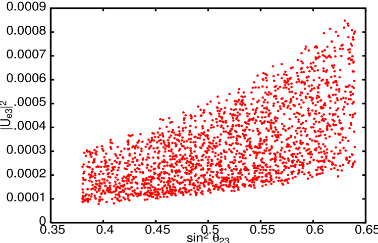
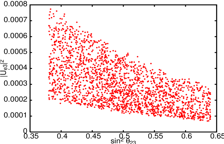
Figure 1: Scatter plot of the correlation between $\sin^{2}\theta_{23}$ and $|U_{e3}|^{2}$ for class $\tilde{B}$ in case of normal hierarchy. All matrices associated with a zero entry in $h_{13}$ generate the same behavior.

Figure 2: Same as above for class $B$. All matrices associated with a zero entry in $h_{12}$ generate the same behavior.

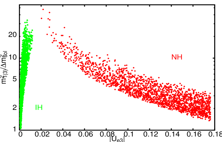
Figure 3: Scatter plot of $|U_{e3}|$ against the ratio of the smallest neutrino mass squared divided by $\Delta m^{2}_{\odot}$ for class $E$, cf. Eqs. (29,31).

Appendix A Group theory of ${D}_{4}$

The group theory is given by the following character table, generator relations and matrices [35]:

	classes
	$\mathcal{C}_{1}$	$\mathcal{C}_{2}$	$\mathcal{C}_{3}$	$\mathcal{C}_{4}$	$\mathcal{C}_{5}$
$\rm G$	$\rm\mathbb{1}$	$\rm A^{2}$	$\rm B$	$\rm AB$	$\rm A$
$\;{}^{\circ}\mathcal{C}_{i}\;$	1	1	2	2	2
$\;{}^{\circ}\mathrm{h}\;_{\mathcal{C}_{i}}$	1	2	2	2	4
$\underline{\mbox{{1}}}_{\mbox{{1}}}$	1	1	1	1	1
$\underline{\mbox{{1}}}_{\mbox{{2}}}$	1	1	-1	1	-1
$\underline{\mbox{{1}}}_{\mbox{{3}}}$	1	1	-1	-1	1
$\underline{\mbox{{1}}}_{\mbox{{4}}}$	1	1	1	-1	-1
$\underline{\mbox{{2}}}$	2	-2	0	0	0

Here we denoted with $\underline{\mbox{{1}}}_{\mbox{{1,2,3,4}}}$ and $\underline{\mbox{{2}}}$ the irreducible representations of ${D}_{4}$, $G$ are the generators of the group, $\;{}^{\circ}\mathcal{C}_{i}\;$ is the order of the class $\mathcal{C}_{i}$ and $\;{}^{\circ}\mathrm{h}\;_{\mathcal{C}_{i}}$ is the order of the elements in class $\mathcal{C}_{i}$, where $i=1,\ldots,5$. The generators $\rm A$ and $\rm B$ for $\underline{\mbox{{2}}}$ are

$$\rm A=\left(\begin{array}[]{cc}0&-1\\ 1&0\end{array}\right)\;\;\;\mbox{and}\;\;\;\rm B=\left(\begin{array}[]{cc}1&0\\ 0&-1\end{array}\right)~{},$$

and fulfill the generator relations

$$\rm A^{4}=\mathbb{1}\;\;\;,\;\;\;B^{2}=\mathbb{1}\;\;\;\mbox{and}\;\;\;ABA=B~{}.$$

From the character table one can read off the Kronecker products:

$\times$	$\underline{\mbox{{1}}}_{\mbox{{1}}}$	$\underline{\mbox{{1}}}_{\mbox{{2}}}$	$\underline{\mbox{{1}}}_{\mbox{{3}}}$	$\underline{\mbox{{1}}}_{\mbox{{4}}}$
$\underline{\mbox{{1}}}_{\mbox{{1}}}$	$\underline{\mbox{{1}}}_{\mbox{{1}}}$	$\underline{\mbox{{1}}}_{\mbox{{2}}}$	$\underline{\mbox{{1}}}_{\mbox{{3}}}$	$\underline{\mbox{{1}}}_{\mbox{{4}}}$
$\underline{\mbox{{1}}}_{\mbox{{2}}}$	$\underline{\mbox{{1}}}_{\mbox{{2}}}$	$\underline{\mbox{{1}}}_{\mbox{{1}}}$	$\underline{\mbox{{1}}}_{\mbox{{4}}}$	$\underline{\mbox{{1}}}_{\mbox{{3}}}$
$\underline{\mbox{{1}}}_{\mbox{{3}}}$	$\underline{\mbox{{1}}}_{\mbox{{3}}}$	$\underline{\mbox{{1}}}_{\mbox{{4}}}$	$\underline{\mbox{{1}}}_{\mbox{{1}}}$	$\underline{\mbox{{1}}}_{\mbox{{2}}}$
$\underline{\mbox{{1}}}_{\mbox{{4}}}$	$\underline{\mbox{{1}}}_{\mbox{{4}}}$	$\underline{\mbox{{1}}}_{\mbox{{3}}}$	$\underline{\mbox{{1}}}_{\mbox{{2}}}$	$\underline{\mbox{{1}}}_{\mbox{{1}}}$

$$\underline{\mbox{{2}}}\times\underline{\mbox{{1}}}_{\mbox{{i}}}=\underline{\mbox{{2}}}\;\;\;\forall\;\rm i~{},~{}\left[\underline{\mbox{{2}}}\times\underline{\mbox{{2}}}\right]=\underline{\mbox{{1}}}_{\mbox{{1}}}+\underline{\mbox{{1}}}_{\mbox{{2}}}+\underline{\mbox{{1}}}_{\mbox{{4}}}~{},~{}\left\{\underline{\mbox{{2}}}\times\underline{\mbox{{2}}}\right\}=\underline{\mbox{{1}}}_{\mbox{{3}}}~{},$$

where $\left[\underline{\mbox{{n}}}\times\underline{\mbox{{n}}}\right]$ denotes the symmetric and $\left\{\underline{\mbox{{n}}}\times\underline{\mbox{{n}}}\right\}$ the anti–symmetric part of the product $\underline{\mbox{{n}}}\times\underline{\mbox{{n}}}$.

The Clebsch–Gordan coefficients for the products $\underline{\mbox{{2}}}\times\underline{\mbox{{1}}}_{\mbox{{i}}}$ are then with $\left(\begin{array}[]{c}s_{1}\\ s_{2}\end{array}\right)\sim\underline{\mbox{{2}}}$ and $t\sim\underline{\mbox{{1}}}_{\mbox{{i}}}$:

$i=1$	$i=2$	$i=3$	$i=4$
$\left(\begin{array}[]{c}s_{1}t\\ s_{2}t\end{array}\right)$	$\left(\begin{array}[]{c}s_{2}t\\ s_{1}t\end{array}\right)$	$\left(\begin{array}[]{c}s_{2}t\\ -s_{1}t\end{array}\right)$	$\left(\begin{array}[]{c}s_{1}t\\ -s_{2}t\end{array}\right)$	$\sim\underline{\mbox{{2}}}$

and for the product $\underline{\mbox{{2}}}\times\underline{\mbox{{2}}}$ for $\left(\begin{array}[]{c}s_{1}\\ s_{2}\end{array}\right),\;\left(\begin{array}[]{c}t_{1}\\ t_{2}\end{array}\right)\sim\underline{\mbox{{2}}}$:

$$(s_{1}t_{1}+s_{2}t_{2})/\sqrt{2}\sim\underline{\mbox{{1}}}_{\mbox{{1}}}\;\;\;\mbox{and}\;\;\;(s_{1}t_{2}+s_{2}t_{1})/\sqrt{2}\sim\underline{\mbox{{1}}}_{\mbox{{2}}}~{},$$

$$(s_{1}t_{2}-s_{2}t_{1})/\sqrt{2}\sim\underline{\mbox{{1}}}_{\mbox{{3}}}\;\;\;\mbox{and}\;\;\;(s_{1}t_{1}-s_{2}t_{2})/\sqrt{2}\sim\underline{\mbox{{1}}}_{\mbox{{4}}}~{}.$$

References

• [1] G. Altarelli and F. Feruglio, New J. Phys.  6, 106 (2004); R. N. Mohapatra et al., hep-ph/0412099; S. T. Petcov, Talk given at the 21st International Conference on Neutrino Physics and Astrophysics (Neutrino 2004), June 14 - 19, 2004, Paris, France, hep-ph/0412410.
• [2] S. W. Barwick et al., astro-ph/0412544.
• [3] C. Aalseth et al., hep-ph/0412300.
• [4] P. Minkowski, Phys. Lett. B67, 421 (1977); T. Yanagida, in Proceedings of the Workshop on Unified Theory and the Baryon Number of the Universe, edited by O. Sawada and A. Sugamoto (KEK, Tsukuba, 1979), p. 95; M. Gell-Mann, P. Ramond, and R. Slansky, in Supergravity, edited by F. van Nieuwenhuizen and D. Freedman (North Holland, Amsterdam, 1979), p. 315; S.L. Glashow, in Quarks and Leptons, edited by M. L$\rm\acute{e}vy$ et al. (Plenum, New York, 1980), p. 707; R.N. Mohapatra and G. Senjanovic, Phys. Rev. Lett. 44, 912 (1980).
• [5] N. Arkani-Hamed et al., Phys. Rev. D 65, 024032 (2002); K. R. Dienes, E. Dudas and T. Gherghetta, Nucl. Phys. B 557, 25 (1999).
• [6] Y. Grossman and M. Neubert, Phys. Lett. B 474, 361 (2000); T. Gherghetta, Phys. Rev. Lett.  92, 161601 (2004); N. Arkani-Hamed and M. Schmaltz, Phys. Rev. D 61, 033005 (2000); G. Barenboim et al., Phys. Rev. D 64, 073005 (2001) P. Q. Hung, Phys. Rev. D 67, 095011 (2003).
• [7] A. Y. Smirnov, Talk given at SEESAW25: International Conference on the Seesaw Mechanism and the Neutrino Mass, Paris, France, 10-11 Jun 2004, hep-ph/0411194; A. de Gouvea, Mod. Phys. Lett. A 19 (2004) 2799.
• [8] H. Murayama, Nucl. Phys. Proc. Suppl.  137, 206 (2004).
• [9] S. Abel, A. Dedes and K. Tamvakis, Phys. Rev. D 71, 033003 (2005); H. Davoudiasl, R. Kitano, G. D. Kribs and H. Murayama, hep-ph/0502176.
• [10] R. N. Mohapatra and J. W. F. Valle, Phys. Rev. D 34, 1642 (1986).
• [11] J. Giedt et al., hep-th/0502032; for small Yukawa couplings in string theories, see also O. J. Eyton-Williams and S. F. King, hep-ph/0502156; S. Antusch, O. J. Eyton-Williams and S. F. King, hep-ph/0505140.
• [12] G. C. Branco and G. Senjanovic, Phys. Rev. D 18, 1621 (1978); D. Chang and R. N. Mohapatra, Phys. Rev. Lett.  58, 1600 (1987); P. Q. Hung, Phys. Rev. D 59, 113008 (1999); hep-ph/0006355.
• [13] J. I. Silva-Marcos, Phys. Rev. D 59, 091301 (1999); I. Gogoladze and A. Perez-Lorenzana, Phys. Rev. D 65, 095011 (2002); Z. Chacko et al., Phys. Rev. D 70, 085008 (2004); C. I. Low, Phys. Rev. D 70, 073013 (2004); H. Davoudiasl et al., hep-ph/0502176.
• [14] M. Fukugita and T. Yanagida, Phys. Lett. B 174, 45 (1986).
• [15] K. Dick et al., Phys. Rev. Lett.  84, 4039 (2000); H. Murayama and A. Pierce, Phys. Rev. Lett.  89, 271601 (2002).
• [16] E. K. Akhmedov, V. A. Rubakov and A. Y. Smirnov, Phys. Rev. Lett.  81, 1359 (1998).
• [17] P. H. Frampton, S. L. Glashow and D. Marfatia, Phys. Lett. B 536, 79 (2002); Z. Z. Xing, Phys. Lett. B 530, 159 (2002); B. R. Desai, D. P. Roy and A. R. Vaucher, Mod. Phys. Lett. A 18, 1355 (2003); W. L. Guo and Z. Z. Xing, Phys. Rev. D 67, 053002 (2003).
• [18] P. H. Frampton, M. C. Oh and T. Yoshikawa, Phys. Rev. D 66, 033007 (2002); A. Kageyama et al., Phys. Lett. B 538, 96 (2002); S. Kaneko, M. Katsumata and M. Tanimoto, JHEP 0307, 025 (2003).
• [19] G. Bhattacharyya, A. Raychaudhuri and A. Sil, Phys. Rev. D 67, 073004 (2003); M. Honda, S. Kaneko and M. Tanimoto, JHEP 0309, 028 (2003); C. Hagedorn, J. Kersten and M. Lindner, Phys. Lett. B 597, 63 (2004).
• [20] B. Pontecorvo, Sov. Phys. JETP 6, 429 (1957) [Zh. Eksp. Teor. Fiz.  33, 549 (1957)]; Sov. Phys. JETP 7, 172 (1958) [Zh. Eksp. Teor. Fiz.  34, 247 (1957)]; Z. Maki, M. Nakagawa and S. Sakata, Prog. Theor. Phys.  28, 870 (1962).
• [21] M. Maltoni et al., New J. Phys.  6, 122 (2004), hep-ph/0405172v4.
• [22] S. M. Bilenky, J. Hosek and S. T. Petcov, Phys. Lett. B 94, 495 (1980); J. Schechter, J. W. F. Valle, Phys. Rev.  D22, 2227 (1980); M. Doi et al., Phys. Lett. B 102, 323 (1981).
• [23] G. C. Branco et al., Phys. Rev. D 67, 073025 (2003); see also G. C. Branco and M. N. Rebelo, New J. Phys.  7, 86 (2005).
• [24] W. Rodejohann, Phys. Rev. D 69, 033005 (2004).
• [25] S. T. Petcov, New J. Phys.  6, 109 (2004).
• [26] W. Rodejohann, Phys. Rev. D 62, 013011 (2000); J. Phys. G 28, 1477 (2002); K. Zuber, hep-ph/0008080; C. S. Lim, E. Takasugi and M. Yoshimura, hep-ph/0411139; A. Atre, V. Barger and T. Han, hep-ph/0502163.
• [27] M. Lindner, M. Ratz, M. A. Schmidt, to appear; M. Lindner, M. A. Schmidt, private communication.
• [28] C. D. Froggatt and H. B. Nielsen, Nucl. Phys. B 147, 277 (1979).
• [29] W. Grimus et al., Eur. Phys. J. C 36, 227 (2004).
• [30] W. Grimus and L. Lavoura, Phys. Lett. B 572, 189 (2003).
• [31] W. Grimus, A. S. Joshipura, S. Kaneko, L. Lavoura and M. Tanimoto, JHEP 0407, 078 (2004).
• [32] M. Frigerio, S. Kaneko, E. Ma and M. Tanimoto, Phys. Rev. D 71, 011901 (2005).
• [33] G. Seidl, hep-ph/0301044.
• [34] See for instance P. H. Frampton and T. W. Kephart, Int. J. Mod. Phys. A 10, 4689 (1995); C. D. Carone and R. F. Lebed, Phys. Rev. D 60, 096002 (1999); P. H. Frampton and A. Rasin, Phys. Lett. B 478, 424 (2000); E. Ma, hep-ph/0409288; K. S. Babu and J. Kubo, hep-ph/0411226; J. Kubo et al., Prog. Theor. Phys.  109, 795 (2003); E. Ma, Phys. Rev. D 61, 033012 (2000); S. L. Chen, M. Frigerio and E. Ma, Phys. Rev. D 70, 073008 (2004) [Erratum-ibid. D 70, 079905 (2004)]; T. Araki, J. Kubo and E. A. Paschos, hep-ph/0502164.
• [35] J. S. Lomont, “Applications of Finite Groups”, Acad. Press (1959) 346 p; M. Hamermesh, “Group Theory and Its Application to Physical Problems”, Reading, Mass.: Addison-Wesley (1962) 509 p.